


1. Introduction
Surface fluxes of momentum and energy through the ocean–atmosphere interface are of primary importance for the characterization of geophysical flows and climate formation mechanisms. Contrary to the case of turbulent wind over land, the presence of a somewhat compliant water surface gives rise to complex nonlinear interaction mechanisms between the atmospheric boundary layer and the wave field developed in response to the turbulent wind forcing itself (Sullivan & McWilliams Reference Sullivan and McWilliams2010). These interactions determine the flux of momentum and energy through the air–sea interface, thus representing a fundamental process for climate behaviour. Despite the relevance of the subject, the physical mechanisms behind wind–wave interactions still lack a sufficiently general and complete theory (Ayet & Chapron Reference Ayet and Chapron2021). The reason is the multiplicity of governing parameters and the lack of suitable experimental and numerical data. As far as it concerns the former, the mechanisms at the basis of wind–wave interactions are influenced by many flow properties, such as the wind intensity, the wind fetch length, the water depth, the water current and the presence of long-wavelength swell waves, to mention a few. The multiplicity of these factors makes the study of the wind–wave problem difficult to rationalize. This aspect is also one of the reasons why we are missing suitable experimental data for the development of sufficiently general and complete theories. Indeed, many field measurements have been performed over ocean and lake surfaces; see e.g. Hristov, Miller & Friehe (Reference Hristov, Miller and Friehe2003), Donelan et al. (Reference Donelan, Babanin, Young and Banner2006) and Laxague & Zappa (Reference Laxague and Zappa2020). Despite the relevance of the information provided, the lack of control on the boundary conditions and in the above-mentioned governing parameters makes the understanding of the observed behaviours rather difficult to rationalize. On the contrary, laboratory experiments provide more detailed information in controlled flow conditions – see e.g. Donelan et al. (Reference Donelan, Haus, Reul, Plant, Stiassnie, Graber, Brown and Saltzman2004), Veron, Saxena & Misra (Reference Veron, Saxena and Misra2007), Buckley & Veron (Reference Buckley and Veron2016, Reference Buckley and Veron2019) – but with obvious limitations in the range of governing parameters covered, especially as far as it concerns the wind fetch length, thus limiting the study to the early-stage development of wind–wave interactions far from equilibrium.
Numerical simulations can avoid some of these issues in principle, but face strong difficulties in solving the two-phase interaction mechanisms at the air–water interface. The issue is essentially given by the numerical treatment of the high jump of the fluid properties occurring at the interface. For this reason, many numerical works avoided this problem by adopting three main strategies. A first category of works elude the numerical solution of the interface by solving problems where the turbulent wind interacts with prescribed and idealized wave patterns. Relevant information has been provided, such as the dependency of the momentum transfer, form drag and scalar transport on the wave properties, including the wave steepness, wave speed and wave age; see e.g. Sullivan, McWilliams & Moeng (Reference Sullivan, McWilliams and Moeng2000), Kihara et al. (Reference Kihara, Hanazaki, Mizuya and Ueda2007), Yang & Shen (Reference Yang and Shen2009, Reference Yang and Shen2010), Druzhinin, Troitskaya & Zilitinkevich (Reference Druzhinin, Troitskaya and Zilitinkevich2012), Yang, Meneveau & Shen (Reference Yang, Meneveau and Shen2013), Sullivan, McWilliams & Patton (Reference Sullivan, McWilliams and Patton2014) and Cao & Shen (Reference Cao and Shen2021). However, the wind–wave interaction problem is simplified extremely by considering monochromatic or broadband travelling waves whose evolution is decoupled from the wind forcing. A second category of works still avoids the solution of the interface by prescribing a wave pattern, but in this case, a wind–wave coupling is considered by solving the wave surface elevation and potential by means of high-order spectral methods. In these cases, the coupling with the wind is taken into account by considering the air pressure distribution over the wave surface, thus allowing for the study of the wave growth and evolution under the action of wind; see e.g. Liu et al. (Reference Liu, Yang, Guo and Shen2010), Hao & Shen (Reference Hao and Shen2019) and Wang et al. (Reference Wang, Zhang, Hao, Huang, Shen, Xu and Zhang2020). The limit of high-order spectral methods is given by the assumption of the water motion as a potential flow where the effects of viscosity, turbulence, surface tension and wave breaking are negligibly small. The third category of works overcomes several of these limits but still eludes the direct solution of the air–water interface. In these works, the problem is split by solving the incompressible Navier–Stokes equations separately in the air and water domains. The coupling between the two solutions is obtained by imposing continuity of velocity and stresses at the deformable interface between the two fluids, and the kinematics of the interface is evaluated using an advection equation for its elevation, thus obtaining the physical deformation of the air and water domains; see e.g. Lin et al. (Reference Lin, Moeng, Tsai, Sullivan and Belcher2008), Zonta, Soldati & Onorato (Reference Zonta, Soldati and Onorato2015) and Li & Shen (Reference Li and Shen2022). In these works, the temporal growth of waves from the initial wind–wave generation processes, and the role played by surface tension and wind strength on the formation of the wave energy spectrum, can be addressed. It is found that the initial linear growth of waves is driven by the convection of the turbulent pressure and by stress fluctuations in accordance with theoretical studies (Phillips Reference Phillips1957). On the other hand, at the later stages, the wave grows exponentially due to the shear flow instability mechanism, again in accordance with theory (Miles Reference Miles1957), and remarkable modifications on the average wind and water profiles are observed.
In accordance with the above arguments, almost the entirety of the numerical works avoided the direct solution of the air–water interface. To our knowledge, the only numerical works where both the wind and water waves are directly resolved are in the context of breaking waves (Yang, Deng & Shen Reference Yang, Deng and Shen2018) and of early-stage transient growth of water waves (Wu, Popinet & Deike Reference Wu, Popinet and Deike2022). The aim of this work is to address the wind–wave interaction problem at equilibrium by solving dynamically the two phases using first principles and a volume of fluid method to reconstruct the interface. What distinguishes the present work is then the fully coupled numerical framework and the reduction of the multiplicity of governing parameters to essentially the sole Reynolds number of the wind. The latter is achieved by considering the statistical symmetries of the flow in an open channel, where the adoption of periodic boundary conditions in the streamwise and spanwise directions allows us to address the wind–wave problem at equilibrium with no effects from the wind fetch that indeed is virtually infinite.
The paper is organized as follows. In § 2, the numerical method and the flow settings are described. In § 3, the water-wave pattern is characterized, while in §§ 4 and 5, the turbulent wind boundary layer is analysed. The influence of the wind–wave mechanisms on the field of stresses in the wind boundary layer is addressed in § 6. Finally, the paper is closed by final remarks in § 7.
2. Direct numerical simulation
2.1. Equations and numerical methods
The evolution of the flow is governed by the continuity and momentum equations. This set of equations is solved here in a one-fluid formulation where the same set of equations is applied for two immiscible fluids with different density  $\rho$ and kinematic viscosity $\nu = \mu /\rho$:
 \begin{equation} \begin{cases} \dfrac{\partial u_i}{\partial x_i} = 0, \\[9pt] \dfrac{\partial \rho u_i}{\partial t} + \dfrac{\partial \rho u_i u_j}{\partial x_j} ={-} \dfrac{\partial p}{\partial x_i} + \dfrac{\partial \tau_{ij}}{\partial x_j} + f_{\sigma_i} + \rho g_i, \end{cases} \end{equation}
where  $u_i$ is the velocity field, $p$ is the pressure field, $\tau _{ij} = 2 \mu {\mathsf{S}}_{ij}$ is the viscous stress tensor with ${\mathsf{S}}_{ij}$ the strain rate tensor, $f_{\sigma _i}$ the surface tension and $g_i$ the acceleration of gravity. In the following, the index $i = 1, 2, 3$ corresponds to the streamwise, vertical and spanwise directions. The OpenFOAM finite volume open source code (Weller et al. Reference Weller, Tabor, Jasak and Fureby1998) has been used to solve numerically the evolution equations. The problem has been discretized numerically by means of a structured Cartesian grid of hexahedral cells. The convective and diffusive fluxes at the numerical volume faces are evaluated through a second-order central difference scheme, whereas time integration is performed with a first-order implicit Euler scheme.
In order to identify the interface between the two fluids, a transport equation for the volume fraction  $\alpha$ (where $\alpha =1$ in the water phase and $\alpha =0$ in the air phase) is coupled with the momentum equation (Hirt & Nichols Reference Hirt and Nichols1981)
 \begin{equation} \frac{\partial \alpha}{\partial t} + \frac{\partial u_j \alpha}{\partial x_j} +\frac{\partial}{\partial x_j} \left[\alpha (1-\alpha ) u_{r_j} \right]= 0. \end{equation}
The numerical challenge of keeping the interface sharp is addressed by limiting the phase fluxes based on the MULES limiter and by using a numerical interface compression method (Deshpande, Anumolu & Trujillo Reference Deshpande, Anumolu and Trujillo2012). The latter is expressed by the last term of (2.2), from which it is easy to recognize that it is active only in the interface region due to the term  $\alpha (1-\alpha )$. In the volume fraction equation (2.2), $\boldsymbol {u_r}$ is a compression velocity evaluated as
 \begin{equation} \boldsymbol{u_r} = c_\alpha \, |\boldsymbol{u}| \, \boldsymbol{\hat{n}}, \end{equation}
where
 \begin{equation} \hat{\boldsymbol{n}} = \frac{\boldsymbol{\nabla}\alpha}{|\boldsymbol{\nabla} \alpha |} \end{equation}
is the unit vector normal to the interface, and  $c_\alpha$ is a compression coefficient that determines the strength of the compression, e.g. $c_\alpha = 0$ for no compression, $c_\alpha = 1$ for conservative compression and $c_\alpha >1$ for high compression (Larsen, Fuhrman & Roenby Reference Larsen, Fuhrman and Roenby2019; Okagaki et al. Reference Okagaki, Yonomoto, Ishigaki and Hirose2021).
The volume fraction  $\alpha$ from (2.2) is then used to compute the physical properties of the two fluids:
 \begin{gather} \rho = \rho_w \alpha +( 1-\alpha ) \rho_a , \end{gather}
 \begin{gather}\mu = \mu_w \alpha + ( 1-\alpha ) \mu_a, \end{gather}
where the subscripts  $w$ and $a$ are used to denote quantities computed for water and air, respectively. The volume fraction $\alpha$ is also used to compute the local curvature of the interface, $\kappa = - \partial n_i / \partial x_i$. This observable is then used to model the surface tension (Brackbill, Kothe & Zemach Reference Brackbill, Kothe and Zemach1992) as
 \begin{equation} f_{\sigma_i} = \sigma \kappa \, \hat{n}_i, \end{equation}
where  $\sigma$ is the surface tension coefficient.
2.2. Fluid properties and compression coefficient
Air and water in standard conditions are considered as working fluids. The corresponding viscosity and density values are  $\nu _a = 1.48 \times 10^{-5}$, $\nu _w = 1 \times 10^{-6}$, $\rho _a = 1$, $\rho _w = 1 \times 10^3$, and the surface tension coefficient is $\sigma = 0.07\ {\rm N}\ {\rm m}^{-1}$. It is important to highlight that the solution of the wind–wave problem based on first-principles equations with the actual properties of air and water represents a challenging task for numerical simulations. Indeed, air and water introduce a high jump of the fluid properties at the interface ( $\rho _w/\rho _a = 1000$ and $\mu _w/\mu _a =67.5$), thus representing an issue for numerical techniques as demonstrated by a series of works where the jump between the two fluid properties has been reduced to obtain numerical stability – see e.g. Liu et al. (Reference Liu, Chong, Yang, Verzicco and Lohse2022) and Scapin, Demou & Brandt (Reference Scapin, Demou and Brandt2022) – or where the evolution of the two fluids is integrated separately in time and their interaction is taken into account with suitable boundary conditions – see e.g. Yang & Shen (Reference Yang and Shen2010, Reference Yang and Shen2011). Here, we succeeded in obtaining a stable solution of the wind–wave problem based on first-principles equations and using the actual properties of air and water. To achieve this result, a relevant role has been played by the value of the compression factor $c_\alpha$ in the volume fraction equation (2.2). Indeed, the value of the compression term is given by the need to obtain a diffusive balance between the artificial diffusion of the numerical method and the negative diffusion of the compression term itself (Larsen et al. Reference Larsen, Fuhrman and Roenby2019; Okagaki et al. Reference Okagaki, Yonomoto, Ishigaki and Hirose2021). In the present case, we found that the intermediate numerical diffusion associated with the use of relatively fine spatial and temporal resolution levels, together with the adoption of mixed first- and second-order-accurate schemes in time and space, can be balanced reasonably by using an intermediate value of the compression coefficient $c_\alpha = 0.5$.
2.3. Flow and simulation settings
The flow case considered is an open channel composed of a water layer on the bottom of an air layer. The origin of the reference frame system is located on top of the water layer, with  $(x,y,z)$ and $(u,v,w)$ denoting the streamwise, vertical and spanwise coordinates and velocity components, respectively. Periodic boundary conditions are applied in the streamwise and spanwise directions. No-slip and free-slip boundary conditions are imposed at the water bed and top boundary, respectively. Finally, a zero gradient condition is imposed in the vertical direction for the volume fraction.
The extent of the numerical domain is  $(L_x, L_y= h_a+h_w, L_z) = (25.6h_a,1.6h_a, 25.6h_a)$, where $h_a$ and $h_w$ are the heights of the air and water portions of the domain. Notice the relatively large domain size adopted with respect to other similar numerical attempts. The reason is given by the need to avoid as much as possible the effects of the finite domain size on the turbulent wind and water-wave statistics, and to improve the statistical convergence of the data with the spatial average. The domain is discretized using a number of volumes $(N_x,N_y,N_z) = (820,277,1232)$ that are distributed homogeneously in the horizontal directions, while stretching laws have been applied in the vertical direction in order to obtain a better resolution in the highly inhomogeneous region around the wind–wave interface. The resulting grid spacing in friction units is $(\Delta x^+, \Delta y_{min}^+, \Delta z^+)=(9.9,0.1,6.6)$, where $\Delta y_{min}^+$ is achieved at the wind–wave interface. Throughout the paper, variables in friction units will be denoted by the superscript +, implying normalization of lengths with the wind friction length $\nu _a / u_{\tau _a}$, and velocities with the wind friction velocity $u_{\tau _a}$. The wind friction velocity $u_{\tau _a}$ is evaluated on top of the interface region between the two fluids as shown in § 5.1 and in Appendix A. On the other hand, when not specifically stated, variables will be reported non-dimensional by using $h_a$ for lengths and $U_e$ for velocities, where $U_e$ is the average velocity at the top boundary. Finally, the time step is variable throughout the simulation to obtain a condition $CFL < 1$ in each point of the domain. The resulting time step is on average $\Delta t^+ =1.1 \times 10^{-4}$.
The evolution of the flow is studied starting from an initial condition where the water column is at rest, the air–water interface is flat and the wind boundary layer is already turbulent. This initial configuration allows us to study the self-development of the water waves under the action of a turbulent wind that in turn adjusts itself to the developing water-wave interface in a fully coupled first-principles framework up to reach statistical equilibrium. The initial condition for the turbulent wind has been taken from a precursory simulation of a single-phase turbulent open channel.
The flow is driven by imposing a constant pressure gradient in the streamwise direction,  ${\rm d}P_b/{{\rm d} x}$. As shown in Appendix A, this pressure gradient determines the friction velocities of both the wind and water boundary layers:
 \begin{equation} u_{\tau_a} \approx \sqrt{- \frac{h_a}{\rho_a}\,\frac{{\rm d} P_b}{{\rm d} x}}, \quad u_{\tau_w} = \sqrt{- \frac{h_w+h_a}{\rho_w}\,\frac{{\rm d} P_b}{{\rm d} x}}, \end{equation}
where  $u_{\tau _a}$ and $u_{\tau _w}$ are the wind and water friction velocities. From the above relations, we have
 \begin{equation} \frac{u_{\tau_a}}{u_{\tau_w}} \approx \frac{1}{\sqrt{1+h_w/h_a}} \, \sqrt{\frac{\rho_w}{\rho_a}}. \end{equation}
Hence, for wind and water boundary-layer heights of the same order,  $h_a \sim {O}(h_w)$, the friction velocity of the wind boundary layer is significantly larger than that attained in the water boundary layer, thus highlighting the tendency of the developed flow set-up in promoting a turbulent wind over an almost quiescent laminar water layer. Accordingly, the ratio of the friction Reynolds numbers in the wind and water boundary layers is fully determined by the heights of the air and water layers:
 \begin{equation} \frac{Re_{\tau_a}}{Re_{\tau_w}} = \frac{\mu_w}{\mu_a} \sqrt{\frac{\rho_a}{\rho_w}} \, \sqrt{\frac{h_a^3}{(h_a+h_w)\,h_w^2}}; \end{equation}
again, see Appendix A. Here,  $Re_{\tau _a} = u_{\tau _a} h_a / \nu _a$ and $Re_{\tau _w} = u_{\tau _w} h_w / \nu _w$ are the friction Reynolds numbers of the air and water boundary layers. In the present flow settings, we have $Re_{\tau _a} = 317$ and a ratio $Re_{\tau _a} / Re_{\tau _w} \approx 3$. In conclusion, the choice of forcing together with the use of periodic boundary conditions allows us to obtain, in a very simple and computationally efficient way, a fully developed turbulent wind boundary layer over an almost quiescent and laminar water layer.
In the present flow settings, the computational demand for well-converged statistics is mitigated by the statistical stationarity of the flow field and by the statistical homogeneity in the streamwise and spanwise directions. Hence the average operator, hereafter denoted as  $\langle {\cdot } \rangle$, combines a spatial average in the horizontal directions and a temporal average over $34$ samples collected every $\Delta T^+= 95$ after reaching a statistically steady state. In what follows, the customary Reynolds decomposition of the flow in a mean and fluctuating field will be adopted, i.e. $u_i = U_i + u_i^\prime$, where capital letters and the prime will denote average and fluctuating quantities, respectively.
2.4. Governing parameters
It is well-known that the wind–wave problem is controlled by several parameters: among many others, we have the intensity of the wind, the wind fetch and the water depth. The combination of these parameters determines the water-wave state and the momentum and heat surface fluxes, e.g. the friction velocity and the heat transfer coefficient of the wind. In the present flow configuration, the wind–wave problem is simplified by the adoption of periodic boundary conditions that remove the dependence of the wind–wave dynamics on the wind fetch being formally infinite. In this idealized framework, the evolution of the flow towards equilibrium is governed by the sole values of the imposed pressure gradient  ${\rm d} P_b / {{\rm d} x}$, of the air boundary-layer thickness $h_a$ and of the water depth $h_w$ being the thermodynamic properties of the fluids prescribed by the selection of air and water as working fluids. From a non-dimensional point of view, by considering the wind friction velocity $u_{\tau _a}$ and the total height of the domain $H=h_a+h_w$ as reference scales, together with the algebraic mean of the two fluid properties $\rho _{ref} =(\rho _a+\rho _w)/2$ and $\mu _{ref} = (\mu _a + \mu _w ) /2$ as reference thermodynamic quantities, the system of equations becomes
 \begin{equation} \begin{cases} \dfrac{\partial u_i^\star}{\partial x_i^\star} = 0, \\[10pt] \displaystyle\frac{\partial \rho^\star u_i^\star}{\partial t^\star} + \frac{\partial \rho^\star u_i^\star u_j^\star}{\partial x_j^\star} ={-}\frac{\partial p^\star}{\partial x_i^\star} + \frac{1}{Re}\,\frac{\partial \tau_{ij}^\star}{\partial x_j^\star} + \frac{1}{We}\,f_{\sigma_i}^\star{+} \frac{1}{Fr^2}\,\rho^\star g_i^\star, \end{cases} \end{equation}
where the governing dimensionless groups are the Reynolds, Weber and Froude numbers defined as
 \begin{equation} Re = \frac{u_{\tau_a} H}{\nu_{ref}}, \quad We = \frac{\rho_{ref} u_{\tau_a}^2 H}{\sigma}, \quad Fr = \frac{u_{\tau_a}}{\sqrt{g H}}, \end{equation}
with  $\nu _{ref} = (\mu _a + \mu _w)/(\rho _a+\rho _w)$. It is then evident that in the present flow settings, the dynamical evolution of the problem from the initial flat water surface to the fully developed turbulent wind over water-wave condition is determined completely by the values of $u_{\tau _a}$ and $H$ that are imposed through the pressure gradient ${\rm d} P_b / {{\rm d} x}$ and the wind- and water-layer heights $h_a$ and $h_w$. The simplicity of these flow settings allows for the development of a theoretical framework (see Appendix A) that allows us to characterize the flow rigorously and to have a full control of the wind and water layers. In particular, the friction Reynolds numbers of the two layers can be varied independently of each other by changes in the pressure gradient ${\rm d} P_b / {{\rm d} x}$ and in the wind- and water-layer heights $h_a$ and $h_w$:
 \begin{equation} Re_{\tau_a} = \frac{h_a}{\nu_a} \sqrt{- \frac{h_a}{\rho_a}\,\frac{{\rm d} P_b}{{\rm d} x}}, \quad Re_{\tau_w} = \frac{h_w}{\nu_w}\sqrt{- \frac{h_w+h_a}{\rho_w}\, \frac{{\rm d} P_b}{{\rm d} x}} . \end{equation}
As already stated, the water waves are not prescribed directly here, being the result of the dynamical evolution of the water phase under the action of the turbulent wind in accordance with (2.11) under a certain value of the triad  $Re$,
$Re$,  $We$ and $Fr$. This triad is controlled directly by the wind friction Reynolds number and by the water/air heights:
 \begin{equation} \left.\begin{gathered} Re = \xi_{Re} \, Re_{\tau_a} \left ( 1 + \frac{h_w}{h_a} \right ), \quad \mbox{with} \ \xi_{Re} = \frac{(1+\rho_w/\rho_a )}{(1+\mu_w/\mu_a )}, \\ We = \xi_{We} \, Re_{\tau_a}^2\,\frac{1}{h_a} \left ( 1 + \frac{h_w}{h_a} \right ), \quad \mbox{with} \ \xi_{We} = \frac{\rho_a \nu_a^2}{2\sigma} \left ( 1 + \frac{\rho_w}{\rho_a} \right ),\\ Fr = \xi_{Fr} \, Re_{\tau_a} \frac{1}{\sqrt{ h_a^3 \left ( 1 + \dfrac{h_w}{h_a} \right )}}, \quad \mbox{with} \ \xi_{Fr} = \frac{\nu_a}{\sqrt{g}}, \end{gathered}\right\} \end{equation}
where  $\xi _{Re}$, $\xi _{We}$ and $\xi _{Fr}$ are values fixed by the selection of air and water as working fluids. Hence, through the values of $\textrm {d} P_b / {\textrm {d} x}$, $h_a$ and $h_w$, we can have a direct control on these relevant parameters for the water waves but not directly on their form. In the present flow settings, we have imposed $Re_{\tau _a} = 317$ and $h_w/h_a = 0.6$, thus leading to
 \begin{equation} Re = 7404, \quad We = 1.007, \quad Fr = 0.00947, \end{equation}
which from a dimensional point of view corresponds to a flow case consisting of a water layer whose depth is 0.15 m on the bottom of a turbulent wind boundary layer with friction velocity  $0.0187\ \textrm {m}\ \textrm {s}^{-1}$ and thickness 0.25 m. The low friction Reynolds number considered, $Re_{\tau _a} = 317$, is given by the computational resources available and obviously limits the results of the present work to the wind–wave phenomena typical of low Reynolds numbers. Indeed, by increasing the Reynolds number, we might expect higher water waves as demonstrated by the direct relation (2.14) between $Re_{\tau _a}$ and the Weber number $We$, which measures how easily the liquid interface can be deformed by the gas phase. Accordingly, the phenomena associated with higher water waves, e.g. the sheltering mechanisms among many others, require higher Reynolds numbers and are left to future investigations.
3. The structure of water waves
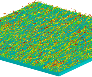
We start the analysis of the direct numerical simulation data by addressing the structure of the water waves. The instantaneous pattern taken by the water waves is shown in figure 1 by means of an iso-surface of the phase fraction  $\alpha = 0.5$. Notice that, for readability reasons, the vertical size of waves has been expanded by a factor of 80. Indeed, the wave height $\delta _w$ is found to be very small compared with both the water depth and the friction length scale of the turbulent wind boundary layer,
 \begin{equation} \left.\begin{gathered} \delta_w =9.2 \times 10^{{-}4}, \\ \delta_w^+= 0.3, \end{gathered}\right\} \end{equation}
where
 \begin{equation} \delta_w = \eta_{max} -\eta_{min}, \end{equation}
with the surface elevation defined as
 \begin{equation} \eta (x,z)= y_\alpha - \langle y_\alpha \rangle, \end{equation}
and  $\alpha (x,y_\alpha,z) = 0.5$. Accordingly, the wave steepness is also very small, $S = 7.3 \times 10^{-4}$. A consequence of the measured very small value of the wave height is that we can drop the dependence of the wave state on the water depth $h_w$. In conclusion, the water-wave evolution here analysed depends uniquely on the selected values of the streamwise pressure gradient $\textrm {d}P_b/{\textrm {d} x}$ and the wind boundary layer thickness $h_a$, i.e. on the friction Reynolds number of the wind $Re_{\tau _a}$. It is important to anticipate here that despite the small height of the water waves, their dynamical effects on the statistical features of the turbulent wind boundary layer are far from being negligible, as will be shown in §§ 4, 5 and 6.
Instantaneous water-wave pattern. The vertical wavelength has been expanded by a factor of 80 for readability reasons. The black arrow denotes the wind direction, the blue line indicates the dominant wave alignment, with  $\gamma$ the angle with respect to the wind direction, and the red arrow indicates the phase speed $\boldsymbol {c}$.

Interestingly, figure 1 shows that the water surface develops an oblique water-wave pattern whose inclination with respect to the streamwise wind direction is  $\gamma = 38.6^\circ$. It is recognized that due to resonance mechanisms of wind–wave generation (Phillips Reference Phillips1957), two dominant wave systems propagate at oblique angles symmetric to the wind direction (Morland Reference Morland1996). This symmetry is, however, often broken for moderate winds, as demonstrated by the present data and by several laboratory and field experiments, e.g. Walsh et al. (Reference Walsh, Hancock, Hines, Swift and Scott1985, Reference Walsh, Hancock, Hines, Swift and Scott1989), Caulliez & Collard (Reference Caulliez and Collard1999), Hwang & Wang (Reference Hwang and Wang2001), Hwang et al. (Reference Hwang, Wang, Yungel, Swift and Krabill2019) and Shemer (Reference Shemer2019), reporting asymmetry in the directional spectra at early stages of wind–waves evolution.
We also observe that the generated oblique wave pattern propagates at an angle in the upstream direction, i.e. the phase speed vector is aligned with the dominant wavenumber of the water waves with a negative streamwise component. In particular, we measure a phase speed  $\boldsymbol {c}^+ \approx (-10, -8)$. Upwind travelling waves have been observed already in the past; see e.g. Plant & Wright (Reference Plant and Wright1980), Hara & Karachintsev (Reference Hara and Karachintsev2003) and Wang & Hwang (Reference Wang and Hwang2004). In accordance with the linear perturbation theory (Plant & Wright Reference Plant and Wright1980), the dependence of the wave propagation direction on the wind shear is odd, while on the wind pressure it is even. Hence wind shear can be thought of as responsible for a downwind propagation of waves together with a water surface drift, while the pressure field can give rise to both upwind and downwind travelling waves. This even effect of pressure is usually broken by the so-called sheltering mechanism of wind separation over the water surface. In fact, field experiments show that upwind travelling waves occur more often in open oceans than in sheltered bays as reported by Wang & Hwang (Reference Wang and Hwang2004). Here, due to the very low steepness of the developed water waves, the wind is able to follow the deformed water surface thus not giving rise to asymmetric pressure distributions in the windward and leeward sides of waves. Hence we argue that the oblique upwind propagation of waves is essentially induced by the pressure field.
From a statistical point of view, this oblique water-wave pattern can be characterized quantitatively by addressing the two-point correlation function of the wave elevation:
 \begin{equation} R_{\eta\eta} (r_x,r_z) = \frac{\langle \eta (x+r_x/2,z+r_z/2, t)\,\eta (x-r_x/2,z-r_z/2,t) \rangle}{\langle \eta^2 \rangle} . \end{equation}
As shown in figure 2, the two-point correlation function exhibits an inclined ( $\gamma \approx 38^\circ$) oscillatory behaviour typical of quasi-periodic phenomena. The distance from the origin of the first positive peak in the correlation along the direction normal to the wave pattern can be used to measure the characteristic wavelength. We measure $\lambda ^+ = 296$. The streamwise and spanwise lengths of this wave pattern are useful for the forthcoming analysis and are measured to be $(\lambda _x^+,\lambda _z^+) = (475,380)$. On the other hand, by rescaling the wavelength with the water depth, we measure $\lambda /h_w = 1.55$. This intermediate value suggests that the developed water waves are mildly influenced by the no-slip condition at the water bed, thus giving further support to the previous assumption that in the present flow settings, the flow state is governed primarily by the friction Reynolds number of the wind $Re_{\tau _a}$ imposed through the pressure gradient $\textrm {d}P_b/{\textrm {d} x}$ and wind boundary layer thickness $h_a$, with a weak dependence on the water depth $h_w$.
Two-point spatial correlation function of the wave elevation  $R_{\eta \eta } (r_x,r_z)$.

The two-point spatial correlation function (3.4) can now be used to compute the one-dimensional spectrum of the wave elevation:
 \begin{equation} \left.\begin{gathered} \hat{E}_{\eta\eta}^x (k_x) = \mathcal{F} \left \{ R_{\eta \eta} (r_x,0) \right \}, \\ \hat{E}_{\eta\eta}^z (k_z) = \mathcal{F} \left \{ R_{\eta \eta} (0,r_z) \right \}, \end{gathered}\right\} \end{equation}
where the operator  $\mathcal {F}$ denotes the Fourier transform. The one-dimensional spectrum allows us to identify the length scales of the most intense waves. As shown in figure 3, both the streamwise and spanwise wave elevation spectra highlight a peak of intensity that is located at streamwise and spanwise wavenumbers that correspond to the wavelengths measured previously with the two-point correlation, i.e. $2{\rm \pi} / k_{x,peak}^+ = 450$ ( $k_{x,peak}^+=1.39 \times 10^{-2}$) and $2{\rm \pi} / k_{z,peak}^+ = 386$ ( $k_{z,peak}^+=1.63 \times 10^{-2}$). Two relevant additional statistical features are, however, evident. The first is given by the presence of a broad range of wavenumbers where the intensity of the wave elevation is not negligible, thus highlighting the occurrence of a multi-scale interface typical of realistic water surfaces. The second is given by the appearance of a secondary peak in the streamwise spectrum at small wavenumbers, $k_x^+ =3.1 \times 10^{-3}$, corresponding to wavelength $2{\rm \pi} / k_{x,peak}^+ =2026$. This secondary peak is a statistical footprint of the presence of group waves (Janssen Reference Janssen2004). Hence the oblique water-wave pattern analysed so far turns out to be superimposed to a longer wave envelope developing in the streamwise direction.
(a) Streamwise and (b) spanwise one-dimensional spectra of the wave elevations  $\hat {E}^x_{\eta \eta }$ and $\hat {E}^z_{\eta \eta }$, respectively.

Let us now address some parameters used classically to characterize the state of water waves. Of particular interest is the so-called Bond number,
 \begin{equation} Bo=\frac{\sigma (2 {\rm \pi}/ \lambda)^2}{\rho_w g}, \end{equation}
which is a measure of the major restoring force between gravity and surface tension. This observable is of particular interest for the present work because the water-wave pattern studied here is not prescribed as in many previous numerical attempts but, rather, is the result of a dynamical evolution from the initial flat surface condition to the equilibrium state with the turbulent wind. Hence, in the present numerical approach, the Bond number turns out to be a result of the flow evolution through the value of the dynamically obtained water-wave length  $\lambda$. With the present flow settings, we measure $Bo \approx 5.1\times 10^{-3}$, thus suggesting a prominent role of gravity as restoring force.
In closing this section, we recall that the described water-wave field is the result of a fully coupled, first-principles evolution of a turbulent wind over a water surface where the unique control parameter is found to be essentially the friction Reynolds number of the wind,  $Re_{\tau _a}$. Accordingly, we may conclude that for a friction Reynolds number $Re_{\tau _a} = 317$, the wind–wave interaction problem develops a wave pattern propagating at an angle in the upwind direction of waves at very low wave steepness and elevation.
4. The structure of the turbulent wind
We consider now the behaviour of the wind boundary layer. Let us recall that the stresses at the water surface created by the wind are responsible for the formation of the previously analysed water-wave pattern that in turn influences the wind boundary layer, thus forming a complex fully coupled mechanism. Hence it is relevant now to address how the physical properties of the turbulent wind are different with respect to classical features observed in wall-bounded turbulence.
4.1. Turbulent coherent motions
In this subsection, we start the study of the turbulent wind by addressing the topology of the turbulent structures populating it. From an instantaneous point of view, coherent vortical structures can be identified by using the so-called  $\lambda _2$ criterion (Jeong et al. Reference Jeong, Hussain, Schoppa and Kim1997), where $\lambda _2$ is the second largest eigenvalue of the tensor
 \begin{equation} {\mathsf{S}}_{ik}{\mathsf{S}}_{kj}+\varOmega_{ik}\varOmega_{kj}, \end{equation}
where  ${\mathsf{S}}_{ij}=(\partial u_i / \partial x_j + \partial u_j / \partial x_i)/2$ and $\varOmega _{ij}=(\partial u_i / \partial x_j - \partial u_j / \partial x_i)/2$ are the symmetric and antisymmetric parts of the velocity gradient tensor. Figure 4 illustrates the iso-surface of $\lambda _2=-3$ coloured with the streamwise velocity, showing that quasi-streamwise vortices are the dominant vortical structures above the wave surface. Consistently with the low elevation and steepness of the water-wave pattern described in § 3, the evolution of the observed quasi-streamwise vortices is essentially not constrained by the water-wave pattern, thus leading to a vortex dynamic that resembles the one observed commonly in wall-bounded turbulence. Such turbulent structures, by interacting with the mean velocity gradient, are known to give rise to streamwise velocity streaks as a result of ejection and sweeping of fluid from/to the near-interface region.
Instantaneous vortex pattern in the turbulent wind boundary layer shown by means of an iso-surface of  $\lambda _2=-3$ coloured with the streamwise velocity.

In order to give a quantitative description of these wind boundary-layer structures and to highlight their statistical relevance, we consider the two-point spatial autocorrelation function of the velocity field,
 \begin{equation} R_{u_i u_i} (\boldsymbol{x}, \boldsymbol{r}) = \frac{\langle\,u_i^\prime (\boldsymbol{x} + \boldsymbol{r},t) u_i^\prime ( \boldsymbol{x},t) \rangle}{\langle u_i^\prime u_i^\prime \rangle (\boldsymbol{x})}, \end{equation}
where no summation is here implied for index  $i$. As seen in figure 5(a), the streamwise correlation function evaluated at $y^+ = 30$ shows that all the three velocity components are correlated over relatively long distances. In particular, we measure correlation lengths $\ell _{x}^+\approx 2800$, $1250$ and $700$ for the streamwise, vertical and spanwise velocity components, respectively. Here, the correlation length is measured as the streamwise spatial increment where $R_{u_i u_i} = 0.05$. These values significantly exceed those reported commonly for wall-bounded turbulence. As an example, by using the turbulent channel database at $Re_\tau = 395$ available online at https://turbulence.oden.utexas.edu, we have that $\ell _{x}^+\approx 1100$, $300$ and $150$ for the streamwise, vertical and spanwise turbulent fluctuations over flat walls at the same wall distance. Hence a significant elongation of the turbulent structures is found to be related to the presence of the water-wave surface. The correlation function in the spanwise direction is shown in figure 5(b). In this case, negative peaks of correlation are observed for the streamwise and vertical velocity components, which can be interpreted as clear statistical evidence of the presence of high and low streamwise velocity streaks and of quasi-streamwise vortices, respectively. In particular, the value of the spanwise scale where these negative peaks occur can be used as a measure of their spanwise size. Accordingly, we measure spanwise spacing between streamwise velocity streaks as $\ell _{z}^+\approx 100$ (location of the negative peak of $R_{uu}$), and spanwise size of quasi-streamwise vortices as $\ell _z^+\approx 53$ (location of the negative peak of $R_{vv}$). These values are again larger than those observed commonly in wall turbulence, where $\ell _{z}^+\approx 70$ and $40$ for the streamwise and vertical turbulent fluctuations at the same wall distance; see again the database available at https://turbulence.oden.utexas.edu.
Two-point spatial autocorrelation function of the velocity field  $R_{u_i u_i}$ computed in the buffer layer region at $y^+ = 30$. (a) Streamwise correlation for $r_y=r_z=0$. (b) Spanwise correlation for $r_x=r_y=0$. The solid line shows $R_{u u}$, the dashed line shows $R_{vv}$ and the dash-dotted line shows $R_{ww}$.

In conclusion, the topology of turbulent structures responsible for the self-sustaining mechanisms of turbulence in the wind boundary layer essentially resembles that observed in classical wall turbulence. The main difference is indeed only of a quantitative nature, as the sizes of the turbulent structures resulting from wind–wave interactions are much larger than those observed in wall-bounded flows. This similarity with wall turbulence is not maintained in the very-near-interface region. There, the effect of the presence of a wind-induced water-wave pattern becomes significant, giving rise to peculiar ordered motions related to the presence of wind–wave interaction phenomena, as will be shown in § 4.2.
4.2. Wave-induced Stokes sublayer and interface stresses
The oblique wave pattern analysed in § 3 is responsible for the appearance of a very interesting phenomenon in the very-near-interface region (say  $y^+ \leqslant 2$). Indeed, it is possible to assume that the air flow, when interacting with the water-wave field, accelerates on the windward side and decelerates on the leeward side. This behaviour can be associated with a pattern for the pressure field that is minimum above the wave crests and maximum within the trough region. As shown in figure 6(a), the instantaneous pressure field actually confirms this scenario by reproducing a pattern that resembles the wave elevation pattern reported for comparison in figure 6(b). Because the water-wave pattern is skewed with respect to the mean wind direction, these pressure variations give rise to periodically distributed pressure gradients in both the streamwise and spanwise directions. Of particular interest is the effect of the latter gradient that is responsible for the generation of an oscillating spanwise forcing, thus inducing an alternating spanwise motion, as shown in figure 7(a). The relevance of this observation is given by the fact that this very-near-interface velocity pattern emulates the flow behaviour of the so-called generalized Stokes layer that is widely recognized to reduce the levels of drag in wall-bounded turbulence (Quadrio, Ricco & Viotti Reference Quadrio, Ricco and Viotti2009; Quadrio & Ricco Reference Quadrio and Ricco2011). As will be shown in § 5, also the present turbulent wind, by interacting with the water-wave field, is characterized by a significant reduction of drag with respect to wall-bounded turbulence. It is then possible to conjecture that this drag reduction is related to the presence of a spanwise oscillating motion induced by the presence of a skewed wave pattern, in analogy with the results obtained in Ghebali, Chernyshenko & Leschziner (Reference Ghebali, Chernyshenko and Leschziner2017) using skewed wavy walls. For this reason, a deeper analysis of the very-near-interface region and the wave-induced Stokes sublayer is reported in the following.
Iso-contours of the instantaneous pressure field  $p^+(x,z)$ evaluated at (a) the water interface $\alpha = 0.5$ and (b) the wave elevation $\eta ^+(x,z)$.

(a) Iso-contours of the instantaneous wave elevation  $\eta ^+(x,z)$ and velocity field streamlines. (b) Iso-contours of the instantaneous spanwise shear $\partial w^+ / \partial y^+ (x,z)$ superimposed onto the iso-levels of the wave elevation $\eta ^+(x,z)$, where positive and negative values are reported with solid and dashed lines, respectively. Both plots show a portion of the entire domain in order to improve the readability of the behaviour.

In contrast with the generalized Stokes layer produced by the spanwise wall motion in active control techniques, the velocity field in the wind–wave case periodically accelerates/decelerates also in the streamwise and vertical direction as a result of the pressure field pattern shown in figure 6(a) and of the wave vertical elevation. However, it is not the velocity field but the associated shear stresses at a given location within the boundary layer that are known to be responsible for the weakening of turbulence, and hence for the consequent drag reduction (Touber & Leschziner Reference Touber and Leschziner2012). As shown in figure 7(b), the instantaneous spanwise shear  $\partial w / \partial y$ at the water surface exhibits an alternating positive and negative behaviour respectively at the wave crest and trough regions. The apparent irregularity of this behaviour is a clear near-interface footprint of the stresses induced by streamwise-aligned turbulent structures populating the wind boundary layer further away from the water surface, as shown in § 4.1.
To clear the analysis of the wave-induced Stokes sublayer from the effects of turbulence structures above it, we introduce a conditional average procedure to address the very-near-interface behaviour separately on the crest and trough wave regions. For the generic quantity  $\beta$, two conditional averages, denoted as $\langle \beta \rangle _\cap$ and $\langle \beta \rangle _\cup$, are computed as the averages over $(x,z)$ points that satisfy the conditions $\eta (x,z,t) > 0.7 \, \delta _w/2$ (crests) and $\eta (x,z,t) < - 0.7 \, \delta _w/2$ (troughs), respectively. As shown in figure 8(a), the flow in the very-near-interface region is characterized by higher streamwise velocity gradients on the crest rather than trough regions, in accordance with the pressure field pattern induced by the water waves. In accordance with this wave-induced pressure field, and as shown in figure 8(b), the mean spanwise velocity gradient exhibits a change of sign moving from the crest to the trough regions. Interestingly, the peaks of streamwise and spanwise shear are located not at the water surface but slightly away from it. This behaviour is related to the interaction of the water surface that, contrary to the generalized Stokes layer induced by moving walls, forms an accelerating/decelerating wave pattern based on first principles. We measure that for the wave-induced Stokes sublayer, the peak of spanwise shear stresses is reached at $y^+ \approx 0.4$ on the wave crests, and at $y^+ \approx 0.25$ on the trough regions. By recalling that the maximum and minimum average values of the wave elevations are $\eta _{max}^+ \approx 0.15$ and $\eta _{min}^+ \approx -0.15$, we can conclude that these peak values are further away from the water surface in the trough regions than in the wave crests; see the vertical lines in figure 8(b).
Very-near-interface behaviour of the crest and trough conditional averages of (a) streamwise shear,  $\langle \partial u / \partial y \rangle _\cap ^+$ (solid line) and $\langle \partial u / \partial y \rangle _\cup ^+$ (dashed line), respectively, and (b) spanwise shear, $\langle \partial w / \partial y \rangle _\cap ^+$ (solid line) and $\langle \partial w / \partial y \rangle _\cup ^+$ (dashed line), respectively. The vertical solid lines denote the average position of the wave crests and troughs.

In closing this section, let us point out that in drag-reducing techniques based on oscillating walls, the thickness of the Stokes layer has been recognized as an important quantity for the effectiveness of the viscous shearing action of the moving wall in weakening the near-wall turbulence interactions (Quadrio & Ricco Reference Quadrio and Ricco2011). For the present wave-induced Stokes sublayer, we measure a penetration length  $\ell _s^+ \approx 2$, computed as the distance from the interface where the conditionally averaged spanwise shear reaches 10 % of its maximum. This value is compatible with a drag-reduction state of the wind boundary layer in accordance with Quadrio & Ricco (Reference Quadrio and Ricco2011), where the minimal condition for drag reduction has been found to be $\ell _s^+ \approx 1$.
To summarize, the very-near-interface field highlights the presence of a wave-induced Stokes sublayer similar to that observed in Ghebali et al. (Reference Ghebali, Chernyshenko and Leschziner2017) for solid skewed wavy walls. The relevance of this layer for the turbulent wind flowing above it is recognized to be in the associated oscillating spanwise motion. The resulting field of spanwise shear takes the form of a streamwise travelling wave whose wavelength and phase speed are as for the water waves, i.e.  $\lambda _x^+ \approx 475$ and $c_x^+ \approx -10$. The intensity of the associated motion and its region of influence are small, $|w|_{max}^+ \approx 10^{-3}$ and $\ell _s^+ \approx 2$, but their effects on the wind boundary layer are not as demonstrated by the level of induced drag reduction reported in § 5.
5. Turbulent wind profiles
The present simulation highlights that the mutual interaction between a water surface and a turbulent wind at a friction Reynolds number  $Re_{\tau _a} = 317$ leads to an inclined pattern of low-steepness waves as shown in § 3. This field of water waves modifies the structure of the turbulent wind as shown in § 4, that in turn created them, thus forming a complex self-sustaining mechanism. Accordingly, it is now relevant to study how and to what degree the statistical features of the turbulent wind are affected by these modified structures with respect to classical behaviours of wall turbulence.
5.1. Mean flow
The effect of moving water waves on the mean wind profile is of overwhelming interest for wind–wave problems in general. In the present flow settings, the interaction of wind with moving waves creates a wave-induced Stokes sublayer that modulates the near-surface flow. It is then important to address if this near-surface modulation affects also the wind flow further away from the water surface, thus leading to a departure from the mean velocity logarithmic law observed classically in wall turbulence. To this aim, we compare the mean velocity profiles from our simulation with those from the simulation of an open channel at  $Re_{\tau }=300$ performed by Nagaosa & Handler (Reference Nagaosa and Handler2003).
Before that, let us point out that the wave elevation pattern makes it essential to define a method to capture the origin of the wind turbulent boundary layer. In analogy with wall turbulence, we define the virtual origin as the location of the maximum of the mean velocity gradient. The resulting location is  $y_0^+=0.37$, i.e. slightly above the water-wave pattern, and the corresponding mean velocity is $U_0^+=0.75$. Following this criterion, the mean velocity profile will be shown by shifting the velocity and the vertical coordinate by $U_0$ and $y_0$, respectively. In the context of the theoretical framework developed in Appendix A, the location $y_0$ corresponds to the upper edge of the interface region ( $\hat {y} = h_{int}^>$ in the reference frame adopted in the appendix). Hence it is the location where the friction velocity of the wind, $u_{\tau _a}$, is computed.
As shown in figure 9, the mean velocity profile is found to follow the classical scalings of the viscous sublayer for  $(y-y_0)^+ < 5$, and of the buffer layer for $(y-y_0)^+ < 20$. However, for $(y-y_0)^+ > 20$, the mean velocity profile is found to deviate from the classical scalings of wall turbulence, especially in the overlap and outer layers. It consists of an upward shift of the mean velocity field with respect to that obtained from wall turbulence in an open channel. This behaviour is consistent with a drag reduction regime of the wind–wave boundary layer with respect to turbulence over smooth walls. This phenomenon of drag reduction can be associated with the presence of the wave-induced Stokes sublayer that in turbulence control techniques is widely recognized to induce a significant drag reduction. From a more quantitative point of view, by assuming a logarithmic behaviour in the putative overlap layer for $30 < (y-y_0)^+ < 0.3 Re_\tau$, i.e.
 \begin{equation}
U^+-U_0^+=\frac{1}{\kappa} \log \left( y^+-y_0^+
\right) + B, \end{equation}
\begin{equation}
U^+-U_0^+=\frac{1}{\kappa} \log \left( y^+-y_0^+
\right) + B, \end{equation}
we measure a small variation of the von Kármán constant  $\kappa =0.38$ for the wind–wave problem with respect to $\kappa _{oc} =0.39$ for wall turbulence in an open channel. On the other hand, the additive constant is found to increase substantially, $B= 7.3$, for the wind–wave problem with respect to $B_{oc}=5.7$ for wall turbulence. Hence the increment $\Delta B = B - B_{oc} = 1.6$ can be interpreted as a measure of the drag reduction experienced by the wind–wave problem with respect to wall turbulence.
Mean wind velocity profile  $(U-U_0)^+$ (solid line) compared with the mean velocity profile of wall turbulence in an open channel (Nagaosa & Handler Reference Nagaosa and Handler2003) (filled circles). The linear law and interpolating logarithmic laws are shown with dashed lines.

By considering the water-wave pattern as a rough surface for the wind boundary layer, we can rewrite the logarithmic law for the mean velocity profile as
 \begin{equation} U^+-U_0^+=\frac{1}{\kappa} \log \left ( \frac{y^+-y_0^+}{k_s^+} \right ) + B_{oc}, \end{equation}
where  $k_s^+$ is an estimate of the surface roughness length, by assuming that the upward shift of the mean velocity profile $\Delta B$ can be modelled as (Pope Reference Pope2000)
 \begin{equation} \Delta B ={-} \frac{1}{\kappa} \log \left( k_s^+ \right). \end{equation}
Accordingly, the effective roughness length of the water surface that is felt by the mean wind boundary layer can be measured as
 \begin{equation} k_s^+= {\rm e}^{- \kappa\,\Delta B} = 0.54, \end{equation}
which is of the same order as the mean wave height  $\delta _w^+ = 0.3$.
5.2. Turbulence intensity profiles
The influence of moving surface waves is also visible in the turbulence intensity profiles as shown in figure 10(a). Compared to wall turbulence, the peak intensity of the streamwise velocity fluctuations is significantly higher and shifted towards the wind boundary-layer core. Also, the peak intensity of the spanwise and vertical velocity fluctuations is moved outwards, but in this case, its magnitude is decreased with respect to wall turbulence. The outward shift of the peaks of turbulent activities is in line with many observations in drag-reducing flows. The modulation of turbulence given by the wave-induced Stokes layer is such that turbulence is weakened in the very-near-interface region. As a consequence, the turbulence self-sustaining mechanisms through which quasi-streamwise vortices and streaks are generated are moved outwards. Indeed, such processes are known to form an autonomous regeneration cycle (Jimenez & Pinelli Reference Jimenez and Pinelli1999) where the presence of the water interface appears to be necessary only to sustain the mean shear. This outward shift allows for the generation of wider and longer velocity streaks, as demonstrated by the two-point correlation function reported in § 4.1. This scenario is consistent with the increase of the intensity of the streamwise velocity fluctuations and with the weakening of the spanwise and vertical velocity fluctuations in the very-near-interface region shown in figure 10(a).
(a) Profiles of wind turbulence intensities (lines) compared with those of wall turbulence in an open channel (circles) (Nagaosa & Handler Reference Nagaosa and Handler2003): streamwise turbulent fluctuations  $\sqrt {\langle u'u' \rangle }$ (solid line), spanwise turbulent fluctuations $\sqrt {\langle w'w' \rangle }$ (dash-dotted line) and vertical turbulent fluctuations $\sqrt {\langle v'v' \rangle }$ (dashed line). (b) Reynolds shear stress $- \langle u'v' \rangle$ profiles in the wind–wave problem (solid line) compared with those of wall turbulence in an open channel (circles) (Nagaosa & Handler Reference Nagaosa and Handler2003). The inset focuses on the behaviour in the near-interface region.

Analogous considerations can be made for the Reynolds shear stresses shown in figure 10(b). The magnitude of  $- \langle u'v' \rangle$ is reduced, and its maximum value is reached for a larger value of $y^+$ with respect to wall turbulence. Interestingly, a change of sign of the Reynolds shear stresses is observed for $y^+ < 1$, as shown in the inset of figure 10(b). This region of the flow represents the wind layer affected directly by the water surface pattern being the wave elevation of the order of $\delta _w^+ = 0.3$, as shown in § 3. Indeed, this change of sign is a clear wave-induced effect. Due to the very low steepness of the water waves ( $S = 7.3 \times 10^{-4}$), the wind is able to remain attached to the water surface, i.e. wind–wave sheltering mechanisms are absent (Jeffreys Reference Jeffreys1925). Accordingly, in the windward side, the flow while raising ( $v'>0$) accelerates in the streamwise direction ( $u'>0$). On the contrary, in the leeward side, the flow while descending ( $v'<0$) decelerates in the streamwise direction ( $u'<0$). Hence both the windward and leeward sides contribute to the production of negative Reynolds shear stresses, $-\langle u'v' \rangle <0$. The present data show that this effect is felt by the wind up to $y^+ = 1$, thus suggesting a penetration length of the wave-induced motions significantly higher than the wave height $\delta _w$ itself. This penetration length is of the same order as that of the wave-induced Stokes sublayer, $\ell _s^+ \approx 2$, thus suggesting the effectiveness of the resulting spanwise oscillating motion in altering the turbulent dynamics of the wind boundary layer.
6. Wind–wave induced fields of stress
Until now, we have addressed the effect of wind–wave interactions on the turbulent wind motions. It is, however, important also to address the fields of stress induced by wind–wave mechanisms. In particular, it is relevant to establish how and to what extent the related fields of stress penetrate into the wind boundary layer. To this aim, we consider the two-point spatial correlation function of pressure and Reynolds shear stresses,
 \begin{equation} R_{pp} (\boldsymbol{x}, \boldsymbol{r}) = \frac{\langle p^\prime (\boldsymbol{x} + \boldsymbol{r},t)\,p^\prime ( \boldsymbol{x},t) \rangle}{\langle p^\prime p^\prime \rangle (\boldsymbol{x})} \end{equation}
and
 \begin{equation} R_{uv} (\boldsymbol{x}, \boldsymbol{r}) = \frac{\langle u^\prime (\boldsymbol{x} + \boldsymbol{r},t)\,v^\prime ( \boldsymbol{x},t) \rangle}{\sqrt{\langle u^\prime u^\prime \rangle (\boldsymbol{x})} \sqrt{\langle v^\prime v^\prime \rangle (\boldsymbol{x})}}, \end{equation}
respectively.
As shown in figure 11, the pressure footprint of the wind–wave interaction mechanisms is felt by the wind boundary layer up to  $y^+\approx 60$ (not shown in figure 11 for readability reasons). It consists of an oscillating behaviour of the two-point pressure correlation. The matching of scales between the water-wave lengths $(\lambda _x^+, \lambda _z^+) = (475,380)$ measured in § 3 and the second peak of pressure correlation suggests clearly that the high- and low-pressure field pattern induced by water waves at their trough and crest (see figure 6) significantly penetrates the wind boundary layer, thus affecting its evolution. It is worth remarking the strongly non-local feature of the pressure field that enables long-distance interactions between a very thin layer of water waves, thickness $\delta _w^+ = 0.3$, with the flow structures populating the wind boundary-layer core.
Two-point spatial autocorrelation function of the pressure field  $R_{pp}$ computed at increasing vertical positions $y^+ = 15$ (solid line), $y^+ = 30$ (dashed line) and $y^+ = 45$ (dash-dotted line). (a) Streamwise correlation for $r_y=r_z=0$. (b) Spanwise correlation for $r_x=r_y=0$.

Contrary to pressure, the turbulent shear stress footprint of the wind–wave interactions does not significantly penetrate into the wind boundary layer and remains more confined in the near-interface region. Indeed, as shown in figure 12, the two-point correlation of Reynolds shear stresses is clearly affected by wind–wave interactions up to  $y^+ \approx 3$, while for $y^+ > 3$, the classical behaviour induced by the structures composing the self-sustaining mechanisms of turbulence is observed, i.e. a negative peak in the spanwise correlation function induced by quasi-streamwise vortices, and streaks at increasingly larger scales by augmenting the distance from the interface.
Two-point spatial correlation function of the Reynolds shear stresses  $R_{uv}$ computed at increasing vertical positions $y^+ = 0.6$ (solid line), $y^+= 1.37$ (dashed line) and $y^+ = 5.37$ (dash-dotted line). (a) Streamwise correlation for $r_y=r_z=0$. (b) Spanwise correlation for $r_x=r_y=0$.

Due to the very low steepness of water waves, the wind boundary layer remains attached to the water surface, hence in the windward side the flow accelerates ( $u' > 0$ and $v' > 0$), while in the leeward side the flow decelerates ( $u' < 0$ and $v' < 0$), in accordance with the near-interface change of sign of the Reynolds shear stresses shown in § 5.2. Accordingly, we may expect a wind–wave footprint in the two-point correlation in the form of a peak of anticorrelation at half water-wave length and a second peak of correlation at the water-wave length itself. Figure 12 actually confirms this scenario up to $y^+ \approx 3$. The clear matching of scales suggests that this region of influence is governed by the wave-induced Stokes sublayer that has been found to have a penetration length of the same order, $\ell _s^+ \approx 2$.
The two-point correlation function of Reynolds shear stresses highlights another remarkable wind–wave feature. Indeed, the peak of correlation for  $y^+ < 3$ occurs for non-zero displacements $(r_x, r_z) = (47, 40)$. This is a clear measure of the phase shift between the streamwise acceleretion/deceleration of the flow ( $u' > 0$ and $u' < 0$) with respect to the windward raising and leeward descending ( $v' > 0$ and $v' < 0$) wave-induced motions. These measured values of shift are of the order of $1/10$ of the water-wave lengths, in accordance with measurements performed by Ghebali et al. (Reference Ghebali, Chernyshenko and Leschziner2017) for solid skewed wavy walls.
7. Conclusions
A direct numerical simulation of the wind–wave interaction problem has been performed. To the authors’ knowledge, the simulation represents one of the very first attempts to obtain the fully coupled solution of the wind–wave problem based on first principles and on realistic values of the fluid properties of air and water. The considered flow settings consist of a two-phase open channel flow driven by a constant pressure gradient where the wind is turbulent and the water is almost quiescent. The simplicity of the flow settings is such that the complex problem of wind turbulence over water waves essentially reduces to be governed by a single parameter, the wind friction Reynolds number  $Re_{\tau _a} = 317$.
The simulation reveals an interesting water-wave pattern. It consists of waves at very low steepness and elevation ( $S = 7.3 \times 10^{-4}$ and $\delta _w^+ = 0.3$) propagating at angle $\gamma = 38.6^\circ$ in the upwind direction with phase speed $\boldsymbol {c}^+ \approx (-10, -8)$. Despite the small size of the water-wave pattern, its effect on the turbulent wind is far from being negligible. A significant reduction of drag is indeed observed, $\Delta B = 1.6$. The origin of drag reduction is associated with the presence of a wave-induced Stokes sublayer. The oblique wave pattern is found to induce periodically distributed pressure gradients also in the spanwise direction, thus leading to an oscillating spanwise forcing. Such a type of modulation gives rise to a weakening of the self-sustaining processes of turbulence in the very-near-interface region, and hence to drag reduction. The significant effect on the turbulent wind is remarkable, despite the very small thickness of the Stokes layer, $\ell _s^+ \approx 2$, and the very weak intensity of the associated motion, $|w|_{max}^+ \approx 10^{-3}$.
Both the mean velocity and turbulent profiles agree with the presence of a near-interface weakening of turbulence due to the wave-induced Stokes sublayer. An upward shift of the self-sustaining processes is indeed observed. A consequence of this shift is the observed increase in size of the main turbulent structures composing the autonomous cycle of turbulence, i.e. quasi-streamwise vortices that are 53 viscous units wide, and streamwise velocity streaks that are 2800 viscous units long. The study of the fields of stress reveals that despite the very small thickness of the Stokes sublayer, its effect on the pressure field is felt in the wind boundary layer also at very large distances from the interface. Indeed, the two-point correlation function clearly highlights the non-local nature of wind–wave induced pressure fluctuations that are shown to penetrate the wind boundary layer up to  $y^+ \approx 60$. On the contrary, the field of shear stresses induced by wind–wave interactions phenomena remains more confined to the water-surface region. These effects emerge in a change of sign of the Reynolds shear stresses $-\langle u'v' \rangle <0$ for $y^+ < 1$ that is clearly induced by the non-sheltering behaviour of the wind over the very low steepness and elevation of the developed water waves. Also, the two-point correlation function confirms this scenario, highlighting that the wind–wave interaction effect on the shear stresses remains confined to the very-near-interface region for $y^+ < 3$.
To close this work, it is important to note that the simulated flow conditions are far from the intense events occurring at the ocean–atmosphere interface. However, the simplicity of the flow settings allows us to reduce the complex problem of wind–wave interactions to its essential features, thus unveiling very basic flow phenomena that may explain some experimental evidence also in real wind–wave problems. An example is the finding of the wave-induced Stokes layer. Such a phenomenon is here unveiled to be at the basis of a change of the momentum flux at the air–water interface. It is then possible to argue that a similar phenomenon can be responsible also for the large scatter of the drag coefficient data in field measurements. Indeed, the condition for the development of the Stokes sublayer is a misalignment of the wind with respect to water waves. In this context, it is well known that field realizations are characterized by the presence of swell waves from remote wind-generation events. Swell waves move in arbitrary directions with respect to the local wind, and their interaction with local wind waves often leads to a water surface pattern that is misaligned with the wind direction. Hence it is reasonable to assume that a Stokes sublayer often develops in field realizations, thus modifying the air–sea momentum flux with respect to that of water waves aligned with the wind that is known to be generally increased with respect to flat surfaces. These arguments suggest analysing field measurements of the drag coefficient as a function of the angle between wind and waves.
Acknowledgements
A.C. and F.R. acknowledge L. Silvestri for his contribution to the preliminary study of this work.
Funding
We wish to acknowledge the financial support given by the Department of Engineering ‘Enzo Ferrari’ of the University of Modena and Reggio Emilia through the action ‘FAR dipartimentale 2020/2021’. The work is also funded by the project ECOSYSTER – SPOKE 6 under the National Recovery and Resilience Plan, Mission 04 Component 2 Investment 1.5 – NextGenerationEU, Call for tender no. 3277 dated 30 December 2021. We acknowledge the Italian supercomputing centre CINECA that, under the ISCRA B project WWW (turbulent Wind and Water Waves interaction: multiscale analysis and modelling) and the ISCRA C project WWIF (simulations of Wind–Wave Interfacial Flows), provided the high-performance computing resources for the present work.
Declaration of interests
The authors report no conflict of interest.
Appendix A. Flow symmetries and mean equations
The configuration of the two-phase open channel considered in the present work exhibits certain statistical symmetries that can be exploited to specialize the mean flow equations. Indeed, by considering fully developed conditions, we have that the average flow solution is invariant under translations in time and in the streamwise and spanwise spatial directions. Furthermore, we have that the average surface tension and also the gravity term have non-zero contributions only in the vertical direction, i.e.  $\langle\,f_{\sigma _1} \rangle = \langle\,f_{\sigma _3} \rangle = 0$ and $\rho g_1 = \rho g_3 = 0$. All these symmetries allow us to reduce the problem of wind–wave interactions to its essential features. The mean flow equations read
 \begin{equation} \begin{cases} \displaystyle\frac{\partial \langle u_i \rangle }{\partial x_i} = 0, \\[9pt] \displaystyle\frac{\partial \langle \rho \rangle \widetilde{u_i}}{\partial t} + \frac{\partial \langle \rho \rangle \widetilde{u_i} \, \widetilde{u_j}}{\partial x_j} ={-}\frac{\partial \langle p \rangle }{\partial x_i} + \frac{\partial \langle \tau_{ij} \rangle}{\partial x_j} - \frac{\partial \langle \rho u_i'' u_j'' \rangle}{\partial x_j}+ \langle\,f_{\sigma_i} \rangle + \langle \rho g_i \rangle, \end{cases} \end{equation}
where the Favre average  $\tilde {\boldsymbol {u}} = \langle \rho \boldsymbol {u} \rangle / \langle \rho \rangle$ and the Favre fluctuation $\boldsymbol {u}'' = \boldsymbol {u} - \tilde {\boldsymbol {u}}$ have been introduced to take into account the density variations at the air–water interface region. By taking into account the above-mentioned statistical symmetries of the flow, the mean flow equations become
 \begin{equation} \begin{cases} \displaystyle\frac{{\rm d} V }{{\rm d} y} = 0, \\[9pt] \displaystyle\frac{{\rm d} \langle \rho \rangle \tilde{u} \, \tilde{v}}{{\rm d} y} ={-}\frac{\partial P}{\partial x} + \frac{{\rm d} \langle \tau_{12} \rangle}{{\rm d} y} - \frac{{\rm d} \langle \rho u'' v'' \rangle}{{\rm d} y}, \\[9pt] \displaystyle\frac{{\rm d} \langle \rho \rangle \tilde{v} \, \tilde{v}}{{\rm d} y} ={-}\frac{\partial P}{\partial y} + \frac{{\rm d} \langle \tau_{22} \rangle}{{\rm d} y} - \frac{{\rm d} \langle \rho v'' v'' \rangle}{{\rm d} y}+ \langle\,f_{\sigma_2} \rangle + \langle \rho g_2 \rangle, \\[9pt] \displaystyle\frac{{\rm d} \langle \rho \rangle \tilde{w} \, \tilde{v}}{{\rm d} y} = \frac{{\rm d} \langle \tau_{32} \rangle}{{\rm d} y} - \frac{{\rm d} \langle \rho w'' v'' \rangle}{{\rm d} y}, \end{cases} \end{equation}
where capital letters are introduced to denote average quantities. From the continuity equation, we have the trivial result  $V= 0$. The above equations (A2) allow us to define the behaviour of the average normal and shear stresses. In the following, to better express the corresponding equations, we consider a shift of the origin of the wall-normal coordinate to the water bed, $\hat {y} = y+h_w$.
By considering the integral of the momentum equation in the vertical direction, we can write an equation for the average pressure field:
 \begin{equation} P = P_b - \langle \rho \rangle \tilde{v} \, \tilde{v} + \langle \tau_{22} \rangle - \langle \rho v''\, v'' \rangle + \int_0^{\hat{y}} \langle\,f_{\sigma_2} \rangle \, {{\rm d} y} + g_2 \int_0^{\hat{y}} \langle \rho \rangle \, {{\rm d} y}, \end{equation}
where  $P_b$ is the average pressure field at the water bed $\hat {y}=0$. An important consequence of this equation is that the mean streamwise pressure gradient is uniform across the two fluids:
 \begin{equation} \frac{\partial P}{\partial x} = \frac{{\rm d}P_b}{{\rm d} x}. \end{equation}
In the vertical stress balance (A3), it is important to highlight that some terms have a non-null contribution only at the interface region between the two fluids. These terms are  $\langle \rho \rangle \tilde {v} \, \tilde {v}$, $\langle \tau _{22} \rangle$ and $\langle\,f_{\sigma _2} \rangle$. Furthermore, outside the interface region, we also have that $\langle \rho \, v'' v'' \rangle$ reduces to the classical Reynolds stress, i.e. $\langle \rho \, v'' v'' \rangle = \langle \rho \, v' v' \rangle$. By taking into account these considerations, we can write
 \begin{equation} P = P_b - \rho_w \langle v' v' \rangle + \rho_w g_2 \, \hat{y} \quad \mbox{for} \ \hat{y} < h_{int}^<, \end{equation}
and
 \begin{align} P &= P_b - \rho_a \langle v' v' \rangle + \int_{h_{int}^<}^{h_{int}^>} \langle\,f_{\sigma_2} \rangle \, {{\rm d} y} + \rho_w g_2 h_{int}^< \nonumber\\ &\quad + \rho_a g_2 \left( \hat{y} - h_{int}^> \right) + g_2 \int_{h_{int}^<}^{h_{int}^>} \langle \rho \rangle \, {{\rm d} y} \quad \mbox{for} \ \hat{y} > h_{int}^>, \end{align}
where  $h_{int}^< < \hat {y} < h_{int}^>$ is the region of the flow where the fluid properties change. The thickness of this layer, $\delta _{int} = h_{int}^> - h_{int}^<$, depends on the height of the wave motion $\delta _w$ and on the thickness of the interface between the two fluids. As the latter is generally small, a good approximation is $\delta _{int} \approx \delta _w$. When the wave elevation is small compared with the height of the air boundary layer $h_a$ and the water depth $h_w$, the thickness of this region is small, $\delta _{int}/h_a \ll 1$ and $\delta _{int}/h_w \ll 1$, thus making the contribution of the two integrals in (A6) generally negligible. Furthermore, the assumptions $\delta _{int}/h_a \ll 1$ and $\delta _{int}/h_w \ll 1$ allow us also to introduce a single interface position, $h_{int} \approx h_{int}^< \approx h_{int}^>$. Hence the vertical stress balances for small water-wave elevations can be finally simplified as
 \begin{equation} \left.\begin{array}{ll} P = P_b - \rho_w \langle v' v' \rangle + \rho_w g_2 \, \hat{y} & \mbox{for} \ \hat{y} < h_{int}, \\[6pt] P = P_b - \rho_a \langle v' v' \rangle + g_2 h_{int} \left [ \rho_w + \rho_a \left( \dfrac{\hat{y}}{h_{int}} - 1 \right ) \right ] & \mbox{for} \ \hat{y} > h_{int}. \end{array}\right\} \end{equation}
We address now the behaviour of the total shear stresses that for the present flow symmetries read
 \begin{equation} T_{12} = \langle \tau_{12} \rangle - \langle \rho \, u'' v''\rangle, \end{equation}
and the streamwise momentum equation (A2) can be recast as
 \begin{equation} \frac{{\rm d} T_{12}}{{\rm d} y} - \frac{{\rm d} \langle \rho \rangle \tilde{u} \, \tilde{v}}{{\rm d} y} = \frac{{\rm d} P_b}{{\rm d} x}, \end{equation}
which integrates to
 \begin{equation} T_{12} - T_{12}^b -\langle \rho \rangle \tilde{u} \, \tilde{v} = \frac{{\rm d} P_b}{{\rm d} x}\,\hat{y}, \end{equation}
where
 \begin{equation} T_{12}^b = \mu_w\,\frac{{\rm d} U}{{\rm d} y} \equiv \rho_w u_{\tau_w}^2 \end{equation}
is the total shear stress at the water bed  $\hat {y}=0$ that can be used to define the friction velocity at the water bed, $u_{\tau _w}^2$. For $\hat {y}=h_w+h_a$, we have $T_{12}=0$ and $\langle \rho \rangle \tilde {u} \, \tilde {v} = 0$, and (A10) allows us to link the imposed streamwise pressure gradient with the friction velocity at the water bed:
 \begin{equation} T_{12}^b ={-} H\,\frac{{\rm d} P_b}{{\rm d} x} \equiv \rho_w u_{\tau_w}^2, \end{equation}
where  $H = ( h_w+h_a )$. Hence the friction velocity at the water bed reads
 \begin{equation} u_{\tau_w} = \sqrt{- \frac{H}{\rho_w}\,\frac{{\rm d} P_b}{{\rm d} x}}. \end{equation}
By considering now  $\hat {y}= h_{int}^>$, we have again that $\langle \rho \rangle \tilde {u} \, \tilde {v} = 0$ and the streamwise stress balance (A10) reduces to
 \begin{equation} T_{12} ={-} h_a\,\frac{{\rm d} P_b}{{\rm d} x} \quad \mbox{for} \ \hat{y} = h_{int}^>, \end{equation}
where (A11) has been used and we have again assumed that  $\delta _{int}/h_a \ll 1$ and $\delta _{int}/h_w \ll 1$, thus allowing us to write the approximation $h_{int}^> - H \approx -h_a$. From (A14), it is possible to derive an equation for the friction velocity at the top edge of the interface region for $\hat {y}= h_{int}^>$. Indeed, at this location, the total shear stress can be recast as
 \begin{equation} T_{12} = \mu_a\,\frac{{\rm d}U}{{\rm d} y} - \rho_a \langle u'v' \rangle \quad \mbox{for} \ \hat{y} = h_{int}^>, \end{equation}
which using (A14), allows us to write
 \begin{equation} \mu_a\,\frac{{\rm d}U}{{\rm d} y} ={-} h_a\,\frac{{\rm d} P_b}{{\rm d} x} + \rho_a \langle u'v' \rangle \quad \mbox{for} \ \hat{y} = h_{int}^>, \end{equation}
where the viscous term can be used to define the friction velocity for the air boundary layer, i.e.
 \begin{equation} \rho_a u_{\tau_a}^2 \equiv \left . \mu_a\,\frac{{\rm d}U}{{\rm d} y}\right |_{\hat{y} = h_{int}^>}. \end{equation}
Hence the friction velocity for the air boundary layer can be computed as
 \begin{equation} u_{\tau_a} = \sqrt{- \frac{h_a}{\rho_a}\,\frac{{\rm d} P_b}{{\rm d} x} + \langle u'v' \rangle}. \end{equation}
In this region of the flow,  $\langle u'v' \rangle$ is essentially due to the wave motion, and by assuming again a small wave elevation, it has a negligible contribution. Hence the friction velocity of the air boundary layer for small water waves can be estimated finally as
 \begin{equation} u_{\tau_a} = \sqrt{- \frac{h_a}{\rho_a}\,\frac{{\rm d} P_b}{{\rm d} x}}, \end{equation}
thus showing the significantly large value attained by the friction velocity for the air flow (indeed turbulent in the present simulation) with respect to that of the water flow (indeed laminar in the present simulation).
It is important now to recall that  $\langle \rho \rangle \tilde {u} \, \tilde {v} = 0$ in the entire flow, except for the thin region $h_{int}^< < \hat {y} < h_{int}^>$ where the fluid properties change. By assuming that
 \begin{equation} |\langle \rho \rangle \tilde{u} \, \tilde{v} | \ll \frac{{\rm d} P_b}{{\rm d} x}\, \hat{y} \end{equation}
also for  $h_{int}^< < \hat {y} < h_{int}^>$, the contribution to the streamwise stress balance (A10) of $\langle \rho \rangle \tilde {u} \, \tilde {v}$ can always be neglected. The inspection of the data from the present simulation supports this assumption. Hence from (A10), we can finally write the behaviour of the total shear stresses as
 \begin{equation} T_{12} ={-} H\,\frac{{\rm d} P_b}{{\rm d} x} \left ( 1- \frac{\hat{y}}{H} \right ), \end{equation}
where again (A11) has been used.


 Open access