1. Introduction
Small-scale, untethered microrobots are attracting increasing interest due to their potential applications in medicine and bioengineering. However, they still face many challenges, such as their mobility and powering (Sitti et al. Reference Sitti, Ceylan, Hu, Giltinan, Turan, Yim and Diller2015; Ceylan et al. Reference Ceylan, Giltinan, Kozielski and Sitti2017). A promising propulsion mechanism is acoustic driving, which, unlike many other approaches, is biocompatible and relatively easy to implement in medical applications. The most common propulsion mechanism for acoustically driven swimmers involves exploiting a gas cavity mounted on the swimmer. Indeed, gas cavities are very good resonators and allow the exploitation of different physical mechanisms for propelling an object (Dijkink et al. Reference Dijkink, Van Der Dennen, Ohl and Prosperetti2006; Ahmed et al. Reference Ahmed, Lu, Nourhani, Lammert, Stratton, Muddana, Crespi and Huang2015; Bertin et al. Reference Bertin, Spelman, Stephan, Gredy, Bouriau, Lauga and Marmottant2015). Attempts to make these swimmers steerable typically involve multiple gas cavities, which results in increased swimmer size (Ahmed et al. Reference Ahmed, Lu, Nourhani, Lammert, Stratton, Muddana, Crespi and Huang2015; Liu & Cho Reference Liu and Cho2021) or reduced propulsion efficiency compared with a monodirectional design (Spelman, Stephan & Marmottant Reference Spelman, Stephan and Marmottant2020). Additionally, bubbles, and thus swimmers equipped with gas cavities (Luo & Wu Reference Luo and Wu2021), are naturally attracted to walls, not only due to lateral forces induced by streaming vortices, but also due to secondary Bjerknes forces between the bubble and its mirror image reflected by the wall.
Some of the drawbacks of swimmers equipped with a gas cavity can be circumvented with entirely solid swimmers. One type of entirely solid swimmers consists of two spheres connected by a spring (Klotsa et al. Reference Klotsa, Baldwin, Hill, Bowley and Swift2015; Dombrowski & Klotsa Reference Dombrowski and Klotsa2020). Another type of solid swimmers are sperm-like objects. A first demonstration of such a sperm-like swimmer was provided by Ahmed et al. (Reference Ahmed, Baasch, Jang, Pane, Dual and Nelson2016), who used a few micrometre-long, axisymmetric objects composed of a rigid head and a flexible tail. The objects were set into resonance at ${90}\,\textrm {kHz}$
, resulting in the propulsion of the swimmer. Larger, sperm-like two-dimensional (2-D) swimmers, of the order of a hundred micrometres and made entirely of polymer, were designed by Kaynak et al. (Reference Kaynak, Ozcelik, Nourhani, Lammert, Crespi and Huang2017). Furthermore, the principle has since been applied to larger, more complex objects (Dillinger, Nama & Ahmed Reference Dillinger, Nama and Ahmed2021). It is generally assumed that the propulsion mechanism is microstreaming induced around the oscillating swimmer. This microstreaming, due to dissipation in the viscous boundary layer, is a relatively slow flow (with respect to the fast acoustic oscillations). While the presence of such flows is indeed supported by experimental evidence (Ahmed et al. Reference Ahmed, Baasch, Jang, Pane, Dual and Nelson2016; Dillinger et al. Reference Dillinger, Nama and Ahmed2021), conducting a repeatable study is challenging, and a detailed understanding of the precise underlying mechanisms is still lacking. Yet, this understanding is essential for further improving the design of such entirely solid swimmers and, most importantly, for addressing their steerability.
${90}\,\textrm {kHz}$
, resulting in the propulsion of the swimmer. Larger, sperm-like two-dimensional (2-D) swimmers, of the order of a hundred micrometres and made entirely of polymer, were designed by Kaynak et al. (Reference Kaynak, Ozcelik, Nourhani, Lammert, Crespi and Huang2017). Furthermore, the principle has since been applied to larger, more complex objects (Dillinger, Nama & Ahmed Reference Dillinger, Nama and Ahmed2021). It is generally assumed that the propulsion mechanism is microstreaming induced around the oscillating swimmer. This microstreaming, due to dissipation in the viscous boundary layer, is a relatively slow flow (with respect to the fast acoustic oscillations). While the presence of such flows is indeed supported by experimental evidence (Ahmed et al. Reference Ahmed, Baasch, Jang, Pane, Dual and Nelson2016; Dillinger et al. Reference Dillinger, Nama and Ahmed2021), conducting a repeatable study is challenging, and a detailed understanding of the precise underlying mechanisms is still lacking. Yet, this understanding is essential for further improving the design of such entirely solid swimmers and, most importantly, for addressing their steerability.
In this paper, we study the microstreaming induced by a vibrating cylindrical cantilever, used as a simple representation of a swimmer tail. One end of cantilever is attached to a vibrating glass support, which is excited by a piezoelectric transducer. A particular interest is devoted to the streaming structures perpendicular to the cantilever axis and to their potential for steering a swimmer.
The streaming around an oscillating cylinder has been widely studied in the past. However, aside from a few exceptions discussed below, these studies generally share two important limitations: (i) the cylinder is typically considered rigid, allowing the system to be simplified to a 2-D problem, and (ii) the cylinder undergoes pure back-and-forth oscillations, which we will refer to as rectilinear oscillations in the following.
Experimental evidence of streaming around a rectilinearly oscillating cylinder was reported as early as the 1930s, both in air (Carrière Reference Carrière1929; Andrade Reference Andrade1931) and in water (Schlichting Reference Schlichting1932). First theoretical considerations by Schlichting (Reference Schlichting1932) were followed by a broader discussion in the early 1950s (Andres & Ingard Reference Andres and Ingard1953a
,Reference Andres and Ingard
b
; Holtsmark et al. Reference Holtsmark, Johnsen, Sikkeland and Skavlem1954; Raney, Corelli & Westervelt Reference Raney, Corelli and Westervelt1954; Westervelt Reference Westervelt1953a
,
Reference Westerveltb
). The main concern at that time was to explain the discrepancies between the different experimental observations. All experiments had recorded streaming patterns divided into four quadrants, which are today known as the typical dipole pattern. However, some experiments reported liquid inflow at the poles (on the $x$
-axis, along the direction of the oscillatory motion) (Carrière Reference Carrière1929; West Reference West1951), while others observed outflow at the poles on the
$x$
-axis, along the direction of the oscillatory motion) (Carrière Reference Carrière1929; West Reference West1951), while others observed outflow at the poles on the $x$
-axis (Schlichting Reference Schlichting1932; West Reference West1951) and yet others identified additional zones of recirculation near the cylinder (Andrade Reference Andrade1931). The seminal theoretical works by Schlichting (Reference Schlichting1932), Holtsmark et al. (Reference Holtsmark, Johnsen, Sikkeland and Skavlem1954) and Raney et al. (Reference Raney, Corelli and Westervelt1954) allow us to understand that the streaming consists of an inner region, with a width of the order of the viscous boundary-layer thickness
$x$
-axis (Schlichting Reference Schlichting1932; West Reference West1951) and yet others identified additional zones of recirculation near the cylinder (Andrade Reference Andrade1931). The seminal theoretical works by Schlichting (Reference Schlichting1932), Holtsmark et al. (Reference Holtsmark, Johnsen, Sikkeland and Skavlem1954) and Raney et al. (Reference Raney, Corelli and Westervelt1954) allow us to understand that the streaming consists of an inner region, with a width of the order of the viscous boundary-layer thickness $\delta$
, and an outer region extending beyond it. The boundary-layer thickness is defined as
$\delta$
, and an outer region extending beyond it. The boundary-layer thickness is defined as $\delta = \sqrt {2\nu /\omega }$
(although some authors use
$\delta = \sqrt {2\nu /\omega }$
(although some authors use $\delta = \sqrt {\nu /\omega }$
), with
$\delta = \sqrt {\nu /\omega }$
), with $\nu$
the kinematic viscosity,
$\nu$
the kinematic viscosity, $\omega$
the angular frequency and the frequency
$\omega$
the angular frequency and the frequency $f = 2\pi \omega$
. More precisely, a universal curve can be found between the ratio
$f = 2\pi \omega$
. More precisely, a universal curve can be found between the ratio $\delta /\!R$
, with
$\delta /\!R$
, with $R$
the radius of the cylinder, and the ratio
$R$
the radius of the cylinder, and the ratio $\delta _{\textit{stream}}/\!R$
, with
$\delta _{\textit{stream}}/\!R$
, with $\delta _{\textit{stream}}$
the thickness of the inner streaming region (Raney et al. Reference Raney, Corelli and Westervelt1954). When
$\delta _{\textit{stream}}$
the thickness of the inner streaming region (Raney et al. Reference Raney, Corelli and Westervelt1954). When $\delta /\!R$
increases,
$\delta /\!R$
increases, $\delta _{\textit{stream}}/\!R$
increases as well. Between the above cited experiments,
$\delta _{\textit{stream}}/\!R$
increases as well. Between the above cited experiments, $\delta /\!R$
varies from negligibly small to dominant in the field of view, which explains the different flow directions. This is also illustrated in figure 1 for a cylinder of a fixed radius of
$\delta /\!R$
varies from negligibly small to dominant in the field of view, which explains the different flow directions. This is also illustrated in figure 1 for a cylinder of a fixed radius of ${100}\,{\unicode{x03BC} \textrm{m}}$
and water viscosity so that the thickness of the inner streaming zones depends only on the frequency. At lower frequencies, the boundary layer is relatively thick, and only the inner streaming region is visible within the field of view. At higher frequencies, the inner region becomes negligibly small, and the outer streaming dominates the field of view. It is noteworthy that the oscillation amplitude does not qualitatively alter the streaming pattern, provided that we remain within the validity of the model, meaning that the amplitude remains small compared with the cylinder radius. Two further important conclusions are reported by Raney et al. (Reference Raney, Corelli and Westervelt1954). Firstly, they propose an additional term to Holtsmark’s model to incorporate Stokes drift, thereby correcting the error caused by describing the cylinder’s motion from a Lagrangian perspective and the flow field from an Eulerian one. Secondly, their experiments confirm the earlier theoretical proof by Westervelt (Reference Westervelt1953a
) that the streaming generated by an oscillating cylinder in a quiescent liquid is equivalent to that generated by an oscillating fluid around a stationary cylinder. For the theoretical streaming to satisfy this result, Stokes drift must be included in the calculations in both reference frames. In parallel, Riley (Reference Riley1965) and others put the calculation of streaming using the method of matched asymptotic expansions onto firm ground. Unlike Holtsmark et al. (Reference Holtsmark, Johnsen, Sikkeland and Skavlem1954), Riley’s work is generally in the limit of small
${100}\,{\unicode{x03BC} \textrm{m}}$
and water viscosity so that the thickness of the inner streaming zones depends only on the frequency. At lower frequencies, the boundary layer is relatively thick, and only the inner streaming region is visible within the field of view. At higher frequencies, the inner region becomes negligibly small, and the outer streaming dominates the field of view. It is noteworthy that the oscillation amplitude does not qualitatively alter the streaming pattern, provided that we remain within the validity of the model, meaning that the amplitude remains small compared with the cylinder radius. Two further important conclusions are reported by Raney et al. (Reference Raney, Corelli and Westervelt1954). Firstly, they propose an additional term to Holtsmark’s model to incorporate Stokes drift, thereby correcting the error caused by describing the cylinder’s motion from a Lagrangian perspective and the flow field from an Eulerian one. Secondly, their experiments confirm the earlier theoretical proof by Westervelt (Reference Westervelt1953a
) that the streaming generated by an oscillating cylinder in a quiescent liquid is equivalent to that generated by an oscillating fluid around a stationary cylinder. For the theoretical streaming to satisfy this result, Stokes drift must be included in the calculations in both reference frames. In parallel, Riley (Reference Riley1965) and others put the calculation of streaming using the method of matched asymptotic expansions onto firm ground. Unlike Holtsmark et al. (Reference Holtsmark, Johnsen, Sikkeland and Skavlem1954), Riley’s work is generally in the limit of small $ \delta / {R}$
(with
$ \delta / {R}$
(with $R$
the cylinder radius), which limits the applicability for low frequencies, but has the advantage of yielding a full analytical solution.
$R$
the cylinder radius), which limits the applicability for low frequencies, but has the advantage of yielding a full analytical solution.

Figure 1. Examples of microstreaming generated around a cylinder undergoing rectilinear oscillations along the horizontal axis. Results are obtained from the model by Holtsmark et al. (Reference Holtsmark, Johnsen, Sikkeland and Skavlem1954) for a cylinder of radius $R=100\,\unicode{x03BC} {\textrm{m}}$
in water (
$R=100\,\unicode{x03BC} {\textrm{m}}$
in water ( $\nu = 10^{-6}\,{\textrm{m}^{2}\, \textrm {s}^{- 1}}$
) and at frequencies
$\nu = 10^{-6}\,{\textrm{m}^{2}\, \textrm {s}^{- 1}}$
) and at frequencies $f = {0.01}, {0.1}, {1}, {10}, {100}\,\textrm {kHz}$
. The corresponding boundary-layer thicknesses are
$f = {0.01}, {0.1}, {1}, {10}, {100}\,\textrm {kHz}$
. The corresponding boundary-layer thicknesses are $\delta ={180},{56},{18},{5.6},{1.8}\,{\unicode{x03BC} \textrm{m}}$
. With
$\delta ={180},{56},{18},{5.6},{1.8}\,{\unicode{x03BC} \textrm{m}}$
. With $R$
and
$R$
and $\nu$
fixed, the extent of the inner streaming structure depends only on the frequency. At
$\nu$
fixed, the extent of the inner streaming structure depends only on the frequency. At ${1}\,\textrm {kHz}$
, both the streaming structure within the boundary layer and the outer streaming are visible. At lower frequencies, only the boundary-layer streaming is visible in the field of view, leading to inflow at the poles on the
${1}\,\textrm {kHz}$
, both the streaming structure within the boundary layer and the outer streaming are visible. At lower frequencies, only the boundary-layer streaming is visible in the field of view, leading to inflow at the poles on the $x$
-axis, whereas at higher frequencies, the outer streaming dominates, resulting in outflow visible at the poles on the
$x$
-axis, whereas at higher frequencies, the outer streaming dominates, resulting in outflow visible at the poles on the $x$
-axis.
$x$
-axis.
While, in the past century, the study of streaming around rectilinearly oscillating cylinders was largely driven by scientific curiosity, it has now become of fundamental interest for practical applications, particularly in microfluidics, for instance in mixing and in the trapping of particles or cells (Lutz, Chen & Schwartz Reference Lutz, Chen and Schwartz2006; Lieu, House & Schwartz Reference Lieu, House and Schwartz2012; Chong et al. Reference Chong, Kelly, Smith and Eldredge2013; House, Lieu & Schwartz Reference House, Lieu and Schwartz2014; Orbay et al. Reference Orbay, Ozcelik, Bachman and Huang2018; Parthasarathy, Chan & Gazzola Reference Parthasarathy, Chan and Gazzola2019). More recently, circular streaming induced by circularly oscillating cylinders has also found applications, such as transporting cells along predefined paths (Hayakawa et al. Reference Hayakawa, Sakuma, Fukuhara, Yokoyama and Arai2014, Reference Hayakawa, Sakuma and Arai2015; Ma et al. Reference Ma, Zhou, Cai, Meng, Zheng and Ai2020).
Theoretically, the problem of circular cylinder motion inducing circular streaming flow was first addressed by Riley (Reference Riley1971), based in part on the work of Longuet-Higgins (Reference Longuet-Higgins1970). In particular, they predicted that no flow reversal between the inner and outer streaming regions, characteristic of rectilinear oscillations (as seen, for example, in figure 1, $f={1}\,\textrm {kHz}$
), would occur. Riley (Reference Riley1992) further developed this theory to account for elliptical motion of the cylinder, with the intent to describe high-Reynolds-number outer streaming for oscillation amplitudes larger than the boundary-layer thickness. For purely circular motion, Hayakawa et al. (Reference Hayakawa, Sakuma, Fukuhara, Yokoyama and Arai2014) later attempted an alternative approach by extending the theory of Holtsmark et al. (Reference Holtsmark, Johnsen, Sikkeland and Skavlem1954). Their model nevertheless contains several typographical errors in the first-order solution and an incorrect mathematical approach for the second order, underlined and corrected here in the supplementary material.
$f={1}\,\textrm {kHz}$
), would occur. Riley (Reference Riley1992) further developed this theory to account for elliptical motion of the cylinder, with the intent to describe high-Reynolds-number outer streaming for oscillation amplitudes larger than the boundary-layer thickness. For purely circular motion, Hayakawa et al. (Reference Hayakawa, Sakuma, Fukuhara, Yokoyama and Arai2014) later attempted an alternative approach by extending the theory of Holtsmark et al. (Reference Holtsmark, Johnsen, Sikkeland and Skavlem1954). Their model nevertheless contains several typographical errors in the first-order solution and an incorrect mathematical approach for the second order, underlined and corrected here in the supplementary material.
To the best of our knowledge, theories for circular motion have not been confronted with experiments, while both reliable theory and corresponding experiments are missing in the elliptical case. Nevertheless, these oscillation modes are essential to understand in the context of micro-swimmers, as they are naturally observed when a cylindrical tail is attached to a vibrating body.
In the present study, we demonstrate that the microstreaming patterns around a vibrating micro-cantilever (used as a model for a micro-swimmer tail) attached to a vibrating substrate can be extremely diverse. This diversity of streaming patterns arises from the broad variety of motion types of the cantilever, including purely rectilinear motion, purely circular motion and various forms of elliptical motion. These results are confronted with a newly developed semi-analytical 2-D model inspired by the original work of Holtsmark et al. (Reference Holtsmark, Johnsen, Sikkeland and Skavlem1954). Unlike previous work, we consider a moving cylinder in a quiescent liquid, not vice versa, and include general elliptical motion, not just rectilinear motion. We evaluate this 2-D model numerically and obtain good agreement with the experiments.
The manuscript is organised as follows. In § 2, we introduce the experimental device, the experimental procedures for microstreaming observations and the measurement of cantilever motion via laser Doppler vibrometry, including the post-processing procedure. The elliptical nature of the recovered cantilever motion emphasises the need for an adequate semi-analytical model, which is derived in § 3. In § 4, we first present the range of cantilever motions obtained, followed by the experimental streaming results and their comparison with the 2-D model. In most of the section, we assume the streaming to be dominantly two-dimensional, but we conclude by discussing the 3-D effects observed, mainly towards the tip of the cantilever. Finally, the manuscript is wrapped up with general conclusions in § 5.
2. Experimental approach
Our experimental device, shown in figure 2 and described in detail in § 2.1, consists of a microscope glass slide excited by a piezoelectric transducer. The aim of this study is to understand the vibrations and the resulting streaming flows of a micro-cantilever attached to the glass slide in the region of interest (ROI). To this end, the experimental procedure follows three steps, (i) the fabrication of the micro-cantilever, described in § 2.2; (ii) the study of the 2-D and 3-D microstreaming, detailed in § 2.3; and (iii) the study of the 3-D micro-cantilever oscillations, presented in § 2.4. The post-processing of the micro-cantilever motion is relatively involved and is explained in detail in § 2.5.

Figure 2. Experimental device and procedures. (a) The experimental device consists of a microscope glass slide to which a piezoelectric transducer was glued. The custom holder (with Polydimethylsiloxane (PDMS) pads for decoupling vibrations from the device) can be mounted on a microscope and a laser Doppler vibrometer. The cantilever was situated in the ROI, which corresponds to the inner wall of the footprint of the PDMS chamber(s). (b) The cantilever was fabricated by filling a PDMS chamber roughly ${600}\,{\unicode{x03BC} \textrm{m}}$
high with PEG-DA and subsequently illuminating it with a circular beam of UV light for polymerisation. (c) Microstreaming experiments are conducted in a
${600}\,{\unicode{x03BC} \textrm{m}}$
high with PEG-DA and subsequently illuminating it with a circular beam of UV light for polymerisation. (c) Microstreaming experiments are conducted in a ${3}\,\textrm {mm}$
-high PDMS chamber filled with water containing tracer particles. (d) Laser doppler vibrometry (LDV) was used to measure the vibrations and displacements of the micro-cantilever in air. A single scan in the
${3}\,\textrm {mm}$
-high PDMS chamber filled with water containing tracer particles. (d) Laser doppler vibrometry (LDV) was used to measure the vibrations and displacements of the micro-cantilever in air. A single scan in the $z$
-direction provides the 1-D profile in that specific direction. To obtain the full 2-D motion, scans along four axes are used. (e) Post-processing enables correlation of the respective micro-cantilever motion with the induced microstreaming patterns. (Schematics not to scale.)
$z$
-direction provides the 1-D profile in that specific direction. To obtain the full 2-D motion, scans along four axes are used. (e) Post-processing enables correlation of the respective micro-cantilever motion with the induced microstreaming patterns. (Schematics not to scale.)
2.1. Preparation of the experimental device
To fabricate the experimental device sketched in figure 2(a), a microscope glass slide ( $76 \times 26 \times {1}\,\textrm {mm}$
, Fisher Scientific) was cleaned in an ultrasound bath, first in acetone, then in isopropanol. It was subsequently oxidised with
$76 \times 26 \times {1}\,\textrm {mm}$
, Fisher Scientific) was cleaned in an ultrasound bath, first in acetone, then in isopropanol. It was subsequently oxidised with $\mathrm{O_2}$
plasma for two minutes at
$\mathrm{O_2}$
plasma for two minutes at ${200}\,\textrm {W}$
to provide a dense layer of reactive silanol groups (
${200}\,\textrm {W}$
to provide a dense layer of reactive silanol groups ( ${\equiv}\textrm {Si}{-}\textrm {OH}$
), which serve as anchoring sites for the adhesion coating. To increase adhesion of the micro-cantilever to the glass surface, we used an organosilane bearing a methacrylate function (3-(Trimethoxysilyl) propyl methacrylate, 98 %, in short TMSPM, Sigma Aldrich). By the technique of self-assembled monolayers, these molecules spontaneously react with the silanol groups on the glass surface, forming a densely packed molecular film (Schreiber Reference Schreiber2000; Onclin, Ravoo & Reinhoudt Reference Onclin, Ravoo and Reinhoudt2005; Aswal et al. Reference Aswal, Lenfant, Guérin, Yakhmi and Vuillaume2006; Ulman Reference Ulman2013). To this end, the freshly cleaned glass substrates were immersed for two hours in a solution of
${\equiv}\textrm {Si}{-}\textrm {OH}$
), which serve as anchoring sites for the adhesion coating. To increase adhesion of the micro-cantilever to the glass surface, we used an organosilane bearing a methacrylate function (3-(Trimethoxysilyl) propyl methacrylate, 98 %, in short TMSPM, Sigma Aldrich). By the technique of self-assembled monolayers, these molecules spontaneously react with the silanol groups on the glass surface, forming a densely packed molecular film (Schreiber Reference Schreiber2000; Onclin, Ravoo & Reinhoudt Reference Onclin, Ravoo and Reinhoudt2005; Aswal et al. Reference Aswal, Lenfant, Guérin, Yakhmi and Vuillaume2006; Ulman Reference Ulman2013). To this end, the freshly cleaned glass substrates were immersed for two hours in a solution of ${100}\,{\unicode{x03BC} \textrm {l}}$
TMSPM and
${100}\,{\unicode{x03BC} \textrm {l}}$
TMSPM and ${100}\,{\unicode{x03BC} \textrm {l}}$
acetic acid (Sigma Aldrich) in
${100}\,{\unicode{x03BC} \textrm {l}}$
acetic acid (Sigma Aldrich) in ${20}\,\textrm {ml}$
toluene (99.8 %, Sigma Aldrich). Finally, the glass slides were thoroughly cleaned in isopropanol, then in dichloromethane by sonication (3 min) and lastly blown dry with nitrogen. The resulting adhesion layer is suitable for promoting covalent bonds with the poly (ethylene glycol) diacrylate (PEG-DA) used for the micro-cantilevers during UV crosslinking.
${20}\,\textrm {ml}$
toluene (99.8 %, Sigma Aldrich). Finally, the glass slides were thoroughly cleaned in isopropanol, then in dichloromethane by sonication (3 min) and lastly blown dry with nitrogen. The resulting adhesion layer is suitable for promoting covalent bonds with the poly (ethylene glycol) diacrylate (PEG-DA) used for the micro-cantilevers during UV crosslinking.
Next, a piezoelectric transducer (RS 724-3162, resonance frequency ${4.2}\,\textrm {kHz}$
) was glued onto the glass slide. Finally, the device was placed in a custom support made of two pieces of Plexiglass held together by two screws. The PDMS pads between the device and the support were used to decouple the device from the holder and prevent vibrations from being transmitted from one to the other. The support could be mounted either on the microscope or the laser Doppler vibrometer without altering the boundary conditions or the resulting constraints on the device.
${4.2}\,\textrm {kHz}$
) was glued onto the glass slide. Finally, the device was placed in a custom support made of two pieces of Plexiglass held together by two screws. The PDMS pads between the device and the support were used to decouple the device from the holder and prevent vibrations from being transmitted from one to the other. The support could be mounted either on the microscope or the laser Doppler vibrometer without altering the boundary conditions or the resulting constraints on the device.
2.2. Fabrication of the micro-cantilever
For the micro-cantilever fabrication (see sketch in figure 2
b), the device was mounted on an optical microscope (Nikon Ti2E) equipped with a UV photopatterning system (Alveole Primo). A PDMS chamber ( ${5}\,\textrm {mm}\times {7}\,\textrm {mm}$
in inner area and approximately
${5}\,\textrm {mm}\times {7}\,\textrm {mm}$
in inner area and approximately ${600}\,{\unicode{x03BC} \textrm{m}}$
in height) was placed in the region of interest and filled with a polymer solution of PEG-DA with an average molecular mass
${600}\,{\unicode{x03BC} \textrm{m}}$
in height) was placed in the region of interest and filled with a polymer solution of PEG-DA with an average molecular mass $M_n = 250$
, mixed with 12 % (w/w) photo-initiator 2-hydroxy-2-methylpropiophenone, as inspired by Orbay et al. (Reference Orbay, Ozcelik, Bachman and Huang2018). A pulse of UV light (
$M_n = 250$
, mixed with 12 % (w/w) photo-initiator 2-hydroxy-2-methylpropiophenone, as inspired by Orbay et al. (Reference Orbay, Ozcelik, Bachman and Huang2018). A pulse of UV light ( ${5}\,{\textrm {mJ}\,\textrm {mm}^{- 2}}$
) was projected through a numerical mask (circular shape, 200 pixels in diameter) of the photopatterning system and a
${5}\,{\textrm {mJ}\,\textrm {mm}^{- 2}}$
) was projected through a numerical mask (circular shape, 200 pixels in diameter) of the photopatterning system and a $20\times$
objective to polymerise the PEG-DA solution within the resulting cylindrical light beam. While the silanised glass slide favours adhesion of the polymerising PEG-DA to the device, a so-called oxygen inhibition layer prevents the PEG-DA from polymerising near the PDMS chamber walls (Dendukuri et al. Reference Dendukuri, Pregibon, Collins, Hatton and Doyle2006). This procedure results in the fabrication of a micro-cantilever approximately
$20\times$
objective to polymerise the PEG-DA solution within the resulting cylindrical light beam. While the silanised glass slide favours adhesion of the polymerising PEG-DA to the device, a so-called oxygen inhibition layer prevents the PEG-DA from polymerising near the PDMS chamber walls (Dendukuri et al. Reference Dendukuri, Pregibon, Collins, Hatton and Doyle2006). This procedure results in the fabrication of a micro-cantilever approximately ${590}\,{\unicode{x03BC} \textrm{m}}$
high and
${590}\,{\unicode{x03BC} \textrm{m}}$
high and ${40}\,{\unicode{x03BC} \textrm{m}}$
in diameter.
${40}\,{\unicode{x03BC} \textrm{m}}$
in diameter.
Care was taken to fabricate the cantilever within a few days after silanising the glass slides, to optimise the adherence of the cantilevers to the device. Immediately after polymerisation, the PDMS chamber was removed, and the region of interest was washed with isopropanol.
2.3. Microstreaming observations
To observe the microstreaming, the device was mounted on the microscope, as shown in the schematic in figure 2(c). A ${3}\,\textrm {mm}$
high PDMS chamber was placed in the region of interest and filled with water containing
${3}\,\textrm {mm}$
high PDMS chamber was placed in the region of interest and filled with water containing ${1}\,{\unicode{x03BC} \textrm{m}}$
tracer particles (red fluorescent polymer microspheres, Duke Scientific). Following the estimations by Barnkob et al. (Reference Barnkob, Augustsson, Laurell and Bruus2012), these particles are sufficiently small to follow the streaming flow, as the influence of radiation forces on their behaviour is negligible. The piezoelectric transducer was connected to a function generator (Tektronix AFG 3102) set to a voltage between
${1}\,{\unicode{x03BC} \textrm{m}}$
tracer particles (red fluorescent polymer microspheres, Duke Scientific). Following the estimations by Barnkob et al. (Reference Barnkob, Augustsson, Laurell and Bruus2012), these particles are sufficiently small to follow the streaming flow, as the influence of radiation forces on their behaviour is negligible. The piezoelectric transducer was connected to a function generator (Tektronix AFG 3102) set to a voltage between ${1}\,\textrm {}$
and
${1}\,\textrm {}$
and ${5}\,\textrm {Vpp}$
, and operated at different frequencies ranging from
${5}\,\textrm {Vpp}$
, and operated at different frequencies ranging from ${30}\,\textrm {}$
to
${30}\,\textrm {}$
to ${300}\,\textrm {kHz}$
. Two different imaging modes were used.
${300}\,\textrm {kHz}$
. Two different imaging modes were used.
The first imaging mode was used for the qualitative visualisation of the microstreaming patterns in 2-D $xy$
-planes parallel to the glass support and perpendicular to the axis of the micro-cantilever. Imaging was ensured with microscope backlighting, a
$xy$
-planes parallel to the glass support and perpendicular to the axis of the micro-cantilever. Imaging was ensured with microscope backlighting, a $20\times$
objective and a high-resolution, high-sensitivity camera (Prime BSI) mounted on the microscope. The camera was operated at a frame rate of
$20\times$
objective and a high-resolution, high-sensitivity camera (Prime BSI) mounted on the microscope. The camera was operated at a frame rate of ${11.8}\,\textrm {fps}$
and controlled via a custom Python script, which directly processed the images. To shorten the duration of the experiments and save memory, the script only stored a superposition of 1000 snapshots, which allows the visualisation of the entire streaming pattern via the ensemble of all the individual tracer particle trajectories. Such images were recorded for different frequencies and at different heights of the micro-cantilever. Three examples are reproduced in figure 3(a). Note that particles up to approximately
${11.8}\,\textrm {fps}$
and controlled via a custom Python script, which directly processed the images. To shorten the duration of the experiments and save memory, the script only stored a superposition of 1000 snapshots, which allows the visualisation of the entire streaming pattern via the ensemble of all the individual tracer particle trajectories. Such images were recorded for different frequencies and at different heights of the micro-cantilever. Three examples are reproduced in figure 3(a). Note that particles up to approximately ${40}\,{\unicode{x03BC} \textrm{m}}$
above or below the focal plane are blurry but visible in the recording. Each recorded image thus corresponds to an ensemble of trajectories over approximately
${40}\,{\unicode{x03BC} \textrm{m}}$
above or below the focal plane are blurry but visible in the recording. Each recorded image thus corresponds to an ensemble of trajectories over approximately ${80}\,{\unicode{x03BC} \textrm{m}}$
in height. For all experiments conducted with this imaging mode, the voltage of the transducer was set to
${80}\,{\unicode{x03BC} \textrm{m}}$
in height. For all experiments conducted with this imaging mode, the voltage of the transducer was set to ${5}\,\textrm {Vpp}$
, as this led to the best image quality.
${5}\,\textrm {Vpp}$
, as this led to the best image quality.

Figure 3. (a) Typical examples of 2-D microstreaming observations. The plots result from a superposition of 1000 snaps hots recorded at a frame rate of ${11.8}\,\textrm {fps}$
. Images are downsampled and contrast-enhanced for a reasonable file size of the manuscript. (b) Three-dimensional tracer particle trajectories (one colour per particle) obtained with the cylindrical lens set-up. The black arrows indicate the flow direction.
${11.8}\,\textrm {fps}$
. Images are downsampled and contrast-enhanced for a reasonable file size of the manuscript. (b) Three-dimensional tracer particle trajectories (one colour per particle) obtained with the cylindrical lens set-up. The black arrows indicate the flow direction.
The second imaging method was used for a quantitative study of the 3-D streaming around the micro-cantilever. To that end, astigmatic imaging with a cylindrical lens, as proposed by Cierpka et al. (Reference Cierpka, Segura, Hain and Kähler2010), was implemented. A camera (IDS U3-3060 CP Rev.2.2), operated at a frame rate of ${5}\,\textrm{fps}$
, was mounted onto the microscope via a camera port adapter (SML20/SM1A44/SM1A39, Thorlabs) containing a cylindrical lens with a focal length of
${5}\,\textrm{fps}$
, was mounted onto the microscope via a camera port adapter (SML20/SM1A44/SM1A39, Thorlabs) containing a cylindrical lens with a focal length of ${150}\,\textrm {mm}$
(LJ1629RM, Thorlabs). Consequently, two focal planes separated by
${150}\,\textrm {mm}$
(LJ1629RM, Thorlabs). Consequently, two focal planes separated by ${40}\,{\unicode{x03BC} \textrm{m}}$
were created, one for the
${40}\,{\unicode{x03BC} \textrm{m}}$
were created, one for the $x$
- and one for the
$x$
- and one for the $y$
-direction. The shape of the particle in the recording changes according to its
$y$
-direction. The shape of the particle in the recording changes according to its $z$
-position relative to these focal planes. Image processing was carried out using DefocusTracker Version 2.0.0 (Rossi & Barnkob Reference Rossi and Barnkob2020; Barnkob & Rossi Reference Barnkob and Rossi2021), which enabled full reconstruction of the 3-D position of each individual particle at every moment in time. During a single recording, particles could only be detected over a height range of approximately
$z$
-position relative to these focal planes. Image processing was carried out using DefocusTracker Version 2.0.0 (Rossi & Barnkob Reference Rossi and Barnkob2020; Barnkob & Rossi Reference Barnkob and Rossi2021), which enabled full reconstruction of the 3-D position of each individual particle at every moment in time. During a single recording, particles could only be detected over a height range of approximately ${140}\,{\unicode{x03BC} \textrm{m}}$
, which is considerably less than the total height of the cantilever. Consequently, data were acquired at several
${140}\,{\unicode{x03BC} \textrm{m}}$
, which is considerably less than the total height of the cantilever. Consequently, data were acquired at several $z$
-planes, spaced by
$z$
-planes, spaced by ${65}\,{\unicode{x03BC} \textrm{m}}$
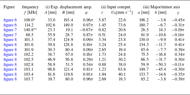
, to cover the entire height of the micro-cantilever and beyond, thereby obtaining a complete 3-D image of the streaming field. Due to the long total acquisition time, such detailed analysis was only conducted for a very limited number of frequencies. Here, we present results for vibrations at
${65}\,{\unicode{x03BC} \textrm{m}}$
, to cover the entire height of the micro-cantilever and beyond, thereby obtaining a complete 3-D image of the streaming field. Due to the long total acquisition time, such detailed analysis was only conducted for a very limited number of frequencies. Here, we present results for vibrations at ${102.5}\,\textrm {kHz}$
, where more than 100 000 velocity vectors in a volume of
${102.5}\,\textrm {kHz}$
, where more than 100 000 velocity vectors in a volume of ${700}\,{\unicode{x03BC} \textrm{m}}\times {700}\,{\unicode{x03BC} \textrm{m}} \times {900}\,{\unicode{x03BC} \textrm{m}}$
around the cantilever were obtained. The corresponding trajectories are shown in figure 3(b). The voltage used in this experiment was set to
${700}\,{\unicode{x03BC} \textrm{m}}\times {700}\,{\unicode{x03BC} \textrm{m}} \times {900}\,{\unicode{x03BC} \textrm{m}}$
around the cantilever were obtained. The corresponding trajectories are shown in figure 3(b). The voltage used in this experiment was set to ${3}\,\textrm {Vpp}$
to optimise the particle displacement between consecutive frames.
${3}\,\textrm {Vpp}$
to optimise the particle displacement between consecutive frames.
Throughout the subsequent analysis of the microstreaming data, a refractive index of 1.3 was used to correct the $z$
-positions in both 2-D and 3-D recordings. For example, if the microscope objective was initially focused on the top of the glass support and then moved upward by
$z$
-positions in both 2-D and 3-D recordings. For example, if the microscope objective was initially focused on the top of the glass support and then moved upward by ${50}\,{\unicode{x03BC} \textrm{m}}$
, the corresponding image plane would be located at an actual height of
${50}\,{\unicode{x03BC} \textrm{m}}$
, the corresponding image plane would be located at an actual height of ${65}\,{\unicode{x03BC} \textrm{m}}$
in the liquid.
${65}\,{\unicode{x03BC} \textrm{m}}$
in the liquid.
2.4. Measurement of the micro-cantilever oscillations
Measurements of the micro-cantilever vibrations were carried out using laser Doppler vibrometry (Polytec PSV-500, equipped with a $10\times$
objective). To this end, the device was positioned so that the micro-cantilever axis was perpendicular to the laser beam (see left schematic in figure 2
d). During the measurement, the piezoelectric transducer was excited by
$10\times$
objective). To this end, the device was positioned so that the micro-cantilever axis was perpendicular to the laser beam (see left schematic in figure 2
d). During the measurement, the piezoelectric transducer was excited by ${128}\,\textrm {ms}$
-long sweeps from
${128}\,\textrm {ms}$
-long sweeps from ${2}\,\textrm {}$
to
${2}\,\textrm {}$
to ${300}\,\textrm {kHz}$
at a voltage of
${300}\,\textrm {kHz}$
at a voltage of ${0.5}\,\textrm {Vpp}$
. The response of the cantilever was recorded using a velocity decoder and the corresponding frequency spectrum obtained via the vibrometer-internal software. Its noise level was reduced by averaging the amplitude and phase (relative to the excitation phase) over 25 sweeps before storing them. Note that, in order to work with vibration amplitudes consistent with those used in the streaming experiments, all data presented in this manuscript have been corrected by a calibration factor of 1000 relative to the raw amplitudes obtained from the frequency sweep of the vibrometer. A detailed justification of this procedure is provided in Appendix B. In brief, it accounts for (i) the vibration amplitude induced by the sweep being much lower than that induced by a pure sine signal at the same voltage, and (ii) the voltages used in the streaming experiments being higher than those applied during the vibration measurements. Furthermore, the amplitudes in water differ from those measured in air. However, as this relationship is far from straightforward, it is not included in the calibration factor but will be addressed separately in § 4.1, and § 4.3.
${0.5}\,\textrm {Vpp}$
. The response of the cantilever was recorded using a velocity decoder and the corresponding frequency spectrum obtained via the vibrometer-internal software. Its noise level was reduced by averaging the amplitude and phase (relative to the excitation phase) over 25 sweeps before storing them. Note that, in order to work with vibration amplitudes consistent with those used in the streaming experiments, all data presented in this manuscript have been corrected by a calibration factor of 1000 relative to the raw amplitudes obtained from the frequency sweep of the vibrometer. A detailed justification of this procedure is provided in Appendix B. In brief, it accounts for (i) the vibration amplitude induced by the sweep being much lower than that induced by a pure sine signal at the same voltage, and (ii) the voltages used in the streaming experiments being higher than those applied during the vibration measurements. Furthermore, the amplitudes in water differ from those measured in air. However, as this relationship is far from straightforward, it is not included in the calibration factor but will be addressed separately in § 4.1, and § 4.3.
A single scan consisted of up to sixty measurement points along the axis of the cantilever. It should be noted that no surface coating is necessary to achieve the measurements, however, the surface of the vibrating object must be (close to) perfectly perpendicular to the incoming laser beam, as otherwise, the reflected beam would not be detected by the vibrometer. This requirement poses a significant challenge for the rounded surface of the cantilever. Consequently, each scan inevitably contained some erroneous points, which were manually discarded when the noise level exceeded ${1.5}\,\textrm {nm}$
. To increase both the reliability and the quantity of our data, the same procedure was therefore repeated up to four times, each time with a slight readjustment of the micro-cantilever’s position relative to the vibrometer head.
${1.5}\,\textrm {nm}$
. To increase both the reliability and the quantity of our data, the same procedure was therefore repeated up to four times, each time with a slight readjustment of the micro-cantilever’s position relative to the vibrometer head.
The procedure described above allows for the recovery of the 1-D motion of multiple points. For example, the schematic on the left of figure 2(d) illustrates the measurement of vibrations in the $y$
-direction. Naturally, each segment of the cantilever generally undergoes a 2-D motion in the
$y$
-direction. Naturally, each segment of the cantilever generally undergoes a 2-D motion in the $xy$
-plane (we consider the
$xy$
-plane (we consider the $z$
-position to be constant), and we shall see that this motion can be described by an ellipse. To reconstruct this elliptical 2-D motion, separate scans along four different axes were conducted, as shown on the right side of figure 2(d). In theory, it is sufficient to correlate the amplitudes and phases of two different scan directions to reconstruct the full motion of the cantilever. However, using a larger number of scans increases the overall robustness and accuracy of the results. The precise post-processing procedure will be discussed in § 2.5.
$z$
-position to be constant), and we shall see that this motion can be described by an ellipse. To reconstruct this elliptical 2-D motion, separate scans along four different axes were conducted, as shown on the right side of figure 2(d). In theory, it is sufficient to correlate the amplitudes and phases of two different scan directions to reconstruct the full motion of the cantilever. However, using a larger number of scans increases the overall robustness and accuracy of the results. The precise post-processing procedure will be discussed in § 2.5.
Additionally, we measured the vibrations of the glass support, once again without special surface coating, in the vicinity of the cantilever to serve as a reference. Naturally, this only provides access to the $z$
-component (the only component we could not measure for the cantilever itself), but it still allows for a comparison of the frequencies corresponding to the vibration maxima between the support and the cantilever.
$z$
-component (the only component we could not measure for the cantilever itself), but it still allows for a comparison of the frequencies corresponding to the vibration maxima between the support and the cantilever.
2.5. Post-processing procedure for recovering the micro-cantilever motion

Figure 4. Reconstruction of the micro-cantilever motion at ${102.8}\,\textrm {kHz}$
. (a) Schematic of the cantilever and the four scanning directions. A full scan along the entire cantilever is illustrated for the
${102.8}\,\textrm {kHz}$
. (a) Schematic of the cantilever and the four scanning directions. A full scan along the entire cantilever is illustrated for the $x$
-direction. (b) Resulting raw amplitudes
$x$
-direction. (b) Resulting raw amplitudes $\xi _i$
and phases
$\xi _i$
and phases $\beta _i$
(with
$\beta _i$
(with $i = x, y, p, m$
) for each scan, using the same colour code as in panel (a). (c) Schematic of the elliptical motion of a single segment
$i = x, y, p, m$
) for each scan, using the same colour code as in panel (a). (c) Schematic of the elliptical motion of a single segment $z_j$
, with the raw amplitudes
$z_j$
, with the raw amplitudes $\xi _i$
, and the final amplitudes
$\xi _i$
, and the final amplitudes $A$
and
$A$
and $B$
. The major axis
$B$
. The major axis $a$
and the minor axis
$a$
and the minor axis $b$
are also indicated. (d) Results for
$b$
are also indicated. (d) Results for $A$
and
$A$
and $B$
and their respective phases
$B$
and their respective phases $\alpha$
and
$\alpha$
and $\varphi$
, obtained from different pairs shown in panel (b). The black and red lines correspond to the averaged values, only the red part is used for the final reconstruction. (e) Final reconstruction: major axis as a function of
$\varphi$
, obtained from different pairs shown in panel (b). The black and red lines correspond to the averaged values, only the red part is used for the final reconstruction. (e) Final reconstruction: major axis as a function of $z$
(left), 3-D representation of the motion over time (centre) and motion of three segments in the
$z$
(left), 3-D representation of the motion over time (centre) and motion of three segments in the $xy$
-plane (right). The three coloured points are the same in each panel.
$xy$
-plane (right). The three coloured points are the same in each panel.
The full reconstruction of the cantilever motion from the vibrometer data is achieved through several post-processing steps, as outlined below. To simplify the explanations, the discussion will be focused on the frequency of ${102.8}\,\textrm {kHz}$
, but the automated procedure can be applied to any frequency of interest, provided that the vibration amplitudes are large enough to yield relevant results.
${102.8}\,\textrm {kHz}$
, but the automated procedure can be applied to any frequency of interest, provided that the vibration amplitudes are large enough to yield relevant results.
-
(i) For all data points, we extract the complex amplitudes $\xi _i \mathrm{e}^{\mathrm{i} \beta _i}$
, where
$\xi _i$
is the real-valued amplitude and
$\beta _i$
the phase. The index
$i$
corresponds to the different directions
$\boldsymbol{e}_x$
,
$\boldsymbol{e}_y$
,
$\boldsymbol{e}_m$
and
$\boldsymbol{e}_p$
, as indicated in figure 4(a). The results for
${102.8}\,\textrm {kHz}$
are shown in figure 4(b). Specifically, the results of twelve scans (two to four per direction) are plotted. Each scan is processed independently of the others in the same direction, as this proved to yield more robust results than averaging at this stage. For the example shown in figure 4(b), the amplitudes for the four scan directions follow a similar trend, and the displacement node around
${500}\,{\unicode{x03BC} \textrm{m}}$
coincides with a phase shift of
$\pi$
, as expected.
$\xi _i \mathrm{e}^{\mathrm{i} \beta _i}$
, where
$\xi _i$
is the real-valued amplitude and
$\beta _i$
the phase. The index
$i$
corresponds to the different directions
$\boldsymbol{e}_x$
,
$\boldsymbol{e}_y$
,
$\boldsymbol{e}_m$
and
$\boldsymbol{e}_p$
, as indicated in figure 4(a). The results for
${102.8}\,\textrm {kHz}$
are shown in figure 4(b). Specifically, the results of twelve scans (two to four per direction) are plotted. Each scan is processed independently of the others in the same direction, as this proved to yield more robust results than averaging at this stage. For the example shown in figure 4(b), the amplitudes for the four scan directions follow a similar trend, and the displacement node around
${500}\,{\unicode{x03BC} \textrm{m}}$
coincides with a phase shift of
$\pi$
, as expected. -
(ii) Initially, the
$z$
-coordinates of the data points do not necessarily coincide between different scans, so that we interpolate the amplitudes and phases onto 40 segments
$z_j$
along the cantilever axis (not shown in the figure). This step is necessary for the subsequent reconstruction. -
(iii) For each interpolation segment
$z_j$
, we thus obtain several sets of data. Each pair of measurements, for example
$\xi _p(z_j)\mathrm{e}^{\mathrm{i}\beta _p(z_j)}$
together with
$\xi _m(z_j)\mathrm{e}^{\mathrm{i}\beta _m(z_j)}$
, is sufficient to describe the elliptical motion of the segment
$z_j$
. Consequently, each pair allows for the reconstruction of the complex amplitudes
$A(z_j)\mathrm{e}^{\mathrm{i}\alpha (z_j)}$
and
$B(z_j)\mathrm{e}^{\mathrm{i}(\alpha (z_j)+\varphi (z_j))}$
along the
$\boldsymbol{e}_x$
and
$\boldsymbol{e}_y$
directions, respectively, as illustrated in figure 4(b). Here,
$A$
and
$B$
are the respective real-valued amplitudes, and
$\varphi$
is the relative phase between the two. The phase
$\alpha$
has no importance for defining the elliptical trajectory, but provides insight into the relative phase of different elements
$z_j$
, such as the
$\pi$
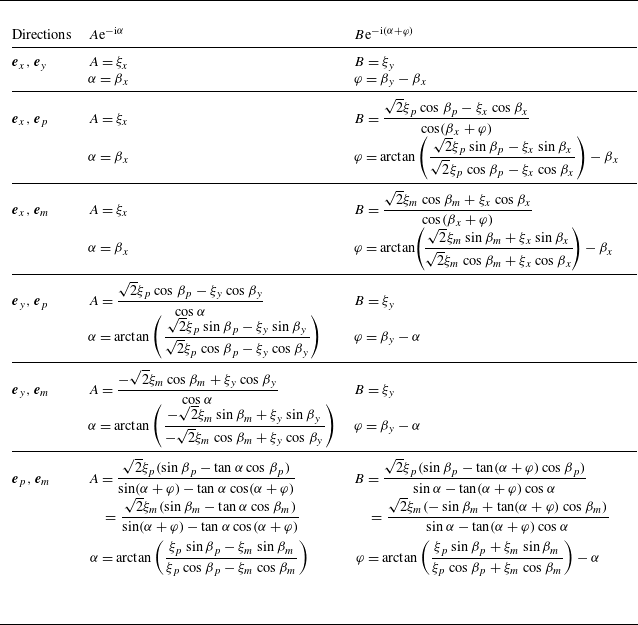
phase shifts corresponding to the amplitude nodes. The full set of equations used for reconstructing the motion from any combination of scan directions is provided in Appendix A. The resulting amplitudes for
${102.8}\,\textrm {kHz}$
are shown as dots in figure 4(d). -
(iv) All results for
$A(z_j)$
,
$\alpha (z_j)$
,
$B(z_j)$
and
$\varphi (z_j)$
are averaged to obtain a single representative value for each segment
$z_j$
, as shown by the black line in figure 4(d). More precisely, we compute the median, which (combined with the use of independently processed scans along the same direction as explained in step (i)) provides the best robustness against inevitable outliers arising from the experimental difficulties. In the following steps, we exclude data points where the total vibration amplitude is too low (i.e. below approximately
${7}\,\textrm {nm}$
, corresponding to five times the accepted noise level), as such points are subject to too large error on the phase. As could already be expected from the raw results, the reconstructed real amplitudes
$A$
and
$B$
for
${102.8}\,\textrm {kHz}$
are of similar magnitude, and the phase shift observed in each
$\xi _i$
naturally reappears in
$\alpha$
. Importantly,
$\varphi$
is approximately
$\pi /2$
, which results in the motion being close to circular rather than purely rectinilear. -
(v) After interpolating or extrapolating missing points, the full motion of the cantilever can be reconstructed, see figure 4(e). The grey lines in the centre plot of figure 4(e) show the elliptical trajectories of each segment
$z_j$
. The three differently coloured ellipses are plotted again in the right plot of figure 4(e) The left panel of figure 4(e) shows a side view of the deformed cantilever, or more precisely, the major axis
$a$
.


In the following, we will limit the representation of the cantilever motion to the two 2-D representations of figure 4(e), namely (I) the major axis $a$
as a function of
$a$
as a function of $z$
, and (II) the elliptical trajectory of a single segment
$z$
, and (II) the elliptical trajectory of a single segment $z_j$
. These two representations fully describe the motion of the cantilever (apart from the offset
$z_j$
. These two representations fully describe the motion of the cantilever (apart from the offset $\alpha$
, which is of no interest here), because all of the ellipses are self-similar within the limits of measurement uncertainty. Indeed, this self-similarity, confirmed by the 3-D representation in figure 4(e) (centre), as well as by the roughly constant ratio
$\alpha$
, which is of no interest here), because all of the ellipses are self-similar within the limits of measurement uncertainty. Indeed, this self-similarity, confirmed by the 3-D representation in figure 4(e) (centre), as well as by the roughly constant ratio $B/A$
and phase
$B/A$
and phase $\varphi$
over
$\varphi$
over $z$
, is a general feature observed at all frequencies, and not specific to the example shown here.
$z$
, is a general feature observed at all frequencies, and not specific to the example shown here.
3. Semi-analytical model of microstreaming
The motion of the micro-cantilever discussed in § 2.5 induces microstreaming in the vicinity of the cantilever when operated in water, as already shown in figure 3. In § 4, we present and discuss the experimental streaming results in detail and, for better understanding, compare them with theoretical expectations. To this end, this section is devoted to developing a semi-analytical 2-D model of the streaming induced by a circular cylinder undergoing elliptical motion in the plane perpendicular to the cylinder axis. A 2-D model is justified because this in-plane motion varies slowly along the length of the cylinder.
Our model builds upon the original work by Holtsmark et al. (Reference Holtsmark, Johnsen, Sikkeland and Skavlem1954), who studied the streaming generated by a stationary cylinder in a rectilinearly oscillating fluid. Further inspired by Hayakawa et al. (Reference Hayakawa, Sakuma, Fukuhara, Yokoyama and Arai2014), who used two $ \pi / 2$
out-of-phase rectilinear oscillations in the
$ \pi / 2$
out-of-phase rectilinear oscillations in the $ x$
- and
$ x$
- and $ y$
-directions to describe circular motion, we generalise this description to include any relative phase and magnitude between the two oscillations. The experimental in-plane, time-harmonic micro-cantilever motion is represented by
$ y$
-directions to describe circular motion, we generalise this description to include any relative phase and magnitude between the two oscillations. The experimental in-plane, time-harmonic micro-cantilever motion is represented by
 \begin{equation} \boldsymbol{\xi } = A \boldsymbol{e}_x \mathrm{e}^{- {\mathrm{i}} \omega t} + B \boldsymbol{e}_y \mathrm{e}^{-{\mathrm{i}} (\omega t + \varphi )} , \end{equation}
where $ \omega$
is the angular frequency and
$ \omega$
is the angular frequency and $A$
and
$A$
and $B$
are real-valued amplitudes. Taking its time derivative, the velocity
$B$
are real-valued amplitudes. Taking its time derivative, the velocity $ \boldsymbol{U}$
of the cylinder is given by
$ \boldsymbol{U}$
of the cylinder is given by
 \begin{equation} \boldsymbol{U} = U_0 \mathrm{e}^{- {\mathrm{i}} \omega t} \big( \boldsymbol{e}_x + \varepsilon \mathrm{e}^{- {\mathrm{i}} \varphi } \boldsymbol{e}_y \big ), \end{equation}
where $ U_0 = - \mathrm{i} \omega A$
is the velocity amplitude in the
$ U_0 = - \mathrm{i} \omega A$
is the velocity amplitude in the $ x$
-direction and
$ x$
-direction and $ \varepsilon U_0 = - \mathrm{i} \omega B$
the velocity amplitude in the
$ \varepsilon U_0 = - \mathrm{i} \omega B$
the velocity amplitude in the $ y$
-direction, which have been introduced for conciseness. Furthermore,
$ y$
-direction, which have been introduced for conciseness. Furthermore, $ \varphi$
represents the relative phase between the two oscillations and
$ \varphi$
represents the relative phase between the two oscillations and $ \varepsilon = B / A$
the relative amplitude. Purely rectilinear motion is obtained in the
$ \varepsilon = B / A$
the relative amplitude. Purely rectilinear motion is obtained in the $ x$
-direction for
$ x$
-direction for $ \varepsilon = 0$
, and purely circular motion is obtained for
$ \varepsilon = 0$
, and purely circular motion is obtained for $ \varepsilon = 1$
and
$ \varepsilon = 1$
and $ \varphi = \pm \pi / 2$
. Many of the remaining combinations of
$ \varphi = \pm \pi / 2$
. Many of the remaining combinations of $ \varepsilon$
and
$ \varepsilon$
and $ \varphi$
yield elliptical motion. Notably, if
$ \varphi$
yield elliptical motion. Notably, if $ \varphi = \pi / 2$
, the major and minor axes of the ellipse coincide with the
$ \varphi = \pi / 2$
, the major and minor axes of the ellipse coincide with the $ x$
- and
$ x$
- and $ y$
-directions, respectively, and
$ y$
-directions, respectively, and $ \varepsilon$
is identical to the amplitude of the minor-axis motion with respect to the major-axis amplitude. Although (3.2) does not include purely rectilinear motion in the
$ \varepsilon$
is identical to the amplitude of the minor-axis motion with respect to the major-axis amplitude. Although (3.2) does not include purely rectilinear motion in the $ y$
-direction, which would correspond
$ y$
-direction, which would correspond $ \varepsilon \to \infty$
, the situation is equivalent to putting
$ \varepsilon \to \infty$
, the situation is equivalent to putting $ \varepsilon = 0$
and rotating the coordinate system by
$ \varepsilon = 0$
and rotating the coordinate system by $ \pi / 2$
.
$ \pi / 2$
.
3.1. Formulation of problem
We represent the micro-cantilever as an infinitely long circular cylinder of radius $ R$
, prescribed with the velocity
$ R$
, prescribed with the velocity $ \boldsymbol{U}$
given by (3.2). On account of the smallness of
$ \boldsymbol{U}$
given by (3.2). On account of the smallness of $ R$
relative to the acoustic wavelength
$ R$
relative to the acoustic wavelength $ \lambda$
,
$ \lambda$
, $ {R} / \lambda \sim 0.001$
, the resulting flow around the cylinder is assumed incompressible. Consequently, the Eulerian flow velocity
$ {R} / \lambda \sim 0.001$
, the resulting flow around the cylinder is assumed incompressible. Consequently, the Eulerian flow velocity $ \boldsymbol{v}$
and vorticity
$ \boldsymbol{v}$
and vorticity $ \boldsymbol{\omega }$
is related to a 2-D streamfunction
$ \boldsymbol{\omega }$
is related to a 2-D streamfunction $ \psi (x, y)$
by
$ \psi (x, y)$
by
 \begin{equation} \boldsymbol{v} = \boldsymbol{\nabla } \times \left ( \psi \boldsymbol{e}_z \right )\! , \quad \boldsymbol{\omega } = \boldsymbol{\nabla }\times \boldsymbol{v} = ( - {\nabla} ^2 \psi ) \boldsymbol{e}_z . \end{equation}
The velocity $ \boldsymbol{v}$
and pressure
$ \boldsymbol{v}$
and pressure $ p$
are governed by the incompressible Navier–Stokes equations
$ p$
are governed by the incompressible Navier–Stokes equations
 \begin{equation} \rho _0 \frac {\partial \boldsymbol{v}}{\partial t} + \rho _0 ( \boldsymbol{v} \boldsymbol{\cdot }\boldsymbol{\nabla } ) \boldsymbol{v} = - \boldsymbol{\nabla }\! p + \eta _0 {\nabla} ^2 \boldsymbol{v} , \end{equation}
where $ \rho _0$
and
$ \rho _0$
and $ \eta _0$
are the density and dynamic viscosity of the fluid, respectively. Equation (3.4) is adjoined by boundary conditions requiring
$ \eta _0$
are the density and dynamic viscosity of the fluid, respectively. Equation (3.4) is adjoined by boundary conditions requiring $ \boldsymbol{v}$
to match
$ \boldsymbol{v}$
to match $ \boldsymbol{U}$
on the surface of the cylinder and to vanish infinitely far away. Expressed in polar coordinates
$ \boldsymbol{U}$
on the surface of the cylinder and to vanish infinitely far away. Expressed in polar coordinates $ (r, \theta )$
, the conditions are
$ (r, \theta )$
, the conditions are
 \begin{align} \boldsymbol{v} & = U_0 \mathrm{e}^{- {\mathrm{i}} \omega t} [ ( \cos \theta + \varepsilon \mathrm{e}^{-{\mathrm{i}} \varphi } \sin \theta ) \boldsymbol{e}_r -( \sin \theta - \varepsilon \mathrm{e}^{-{\mathrm{i}} \varphi } \cos \theta ) \boldsymbol{e}_\theta ] \quad && \text{on cylinder} , \end{align}
 \begin{align} \boldsymbol{v} & \to \boldsymbol{0} \quad && \text{far away}. \end{align}
Taking the curl of (3.4) and using (3.3), the $ z$
-component of the resulting vorticity equation constitutes an equation for
$ z$
-component of the resulting vorticity equation constitutes an equation for $ \psi$
 \begin{equation} \left ( {\nabla} ^2 - \frac {1}{\nu _0} \frac {\partial }{\partial t} \right ) {\nabla} ^2 \psi = \frac {1}{\nu _0} \left ( \boldsymbol{v} \boldsymbol{\cdot }\boldsymbol{\nabla } \right ) ( {\nabla} ^2 \psi ) , \end{equation}
where $ \nu _0 = \eta _0 / \rho _0$
is the kinematic viscosity.
$ \nu _0 = \eta _0 / \rho _0$
is the kinematic viscosity.
Equation (3.6) is solved under the assumption of small oscillation amplitudes defined as
 \begin{equation} \epsilon = \frac {U_0}{\omega {R}} \ll 1 , \end{equation}
which is justified by the reasonably small $ \epsilon \approx 0.005$
found for the typical experimental values
$ \epsilon \approx 0.005$
found for the typical experimental values $ {R} = {20}\,{\unicode{x03BC} \textrm{m}}$
,
$ {R} = {20}\,{\unicode{x03BC} \textrm{m}}$
, $ f = {100}\,{\textrm {k}\textrm {Hz}}$
and
$ f = {100}\,{\textrm {k}\textrm {Hz}}$
and $ U_{0} = {0.06}\,{\textrm{m}\,\textrm {s}^{-1}}$
. The flow fields are written as perturbation expansions up to second order in
$ U_{0} = {0.06}\,{\textrm{m}\,\textrm {s}^{-1}}$
. The flow fields are written as perturbation expansions up to second order in $ \epsilon$
 \begin{align} \psi & = \psi _{1} + \psi _{2} , \end{align}
 \begin{align} \boldsymbol{v} & = \boldsymbol{v}_1 + \boldsymbol{v}_2 , \end{align}
where the first-order fields describe the linear response of the fluid to the motion of the cylinder, and the second-order fields describe the lowest-order nonlinear response, which includes the experimentally observed steady microstreaming as well as a time-harmonic microstreaming at twice the frequency, which is unresolved in the experiments.
Our problem is similar to that of Holtsmark et al. (Reference Holtsmark, Johnsen, Sikkeland and Skavlem1954), but with the modified boundary conditions given in (3.5) and in the frame of reference of an oscillating cylinder in a fluid otherwise at rest. As demonstrated by Westervelt (Reference Westervelt1953a ), the second-order streaming is invariant to a coordinate transformation that renders the cylinder stationary and the fluid oscillating. This evident mathematical similarity between the two situations allows us to solve the problem by following steps similar to those of Holtsmark et al. (Reference Holtsmark, Johnsen, Sikkeland and Skavlem1954). While we briefly outline these steps here, more detailed explanations can be found in the earlier work.
3.2. Calculation of the first-order flow fields
To first order, (3.6) is
 \begin{equation} \big( {\nabla} ^2 + k_{{s}}^{2} \big) {\nabla} ^2 \psi _{1} = 0 , \quad \text{with} \quad k_{{s}} = \frac {1 + \mathrm{i}}{\delta } \quad \text{and} \quad \delta = \sqrt {\frac {2 \nu _0}{\omega }} , \end{equation}
where $ k_{{s}}$
and
$ k_{{s}}$
and $ \delta$
are the shear wavenumber and the viscous boundary-layer thickness. The corresponding boundary conditions are
$ \delta$
are the shear wavenumber and the viscous boundary-layer thickness. The corresponding boundary conditions are
 \begin{align} r^{-1} \partial _\theta \psi _{1} & = U_0 ( \cos \theta + \varepsilon \mathrm{e}^{-{\mathrm{i}} \varphi } \sin \theta ) \quad && \text{for } r = {R} , \end{align}
 \begin{align} - \partial _r \psi _{1} & = - U_0 ( \sin \theta - \varepsilon \mathrm{e}^{-{\mathrm{i}} \varphi } \cos \theta ) \quad && \text{for } r = {R} , \end{align}
 \begin{align} r^{-1} \partial _\theta \psi _{1} & \to 0 \quad && \text{for } r \to \infty , \end{align}
 \begin{align} - \partial _r \psi _{1} & \to 0 \quad && \text{for } r \to \infty . \end{align}
Following Holtsmark et al. (Reference Holtsmark, Johnsen, Sikkeland and Skavlem1954), but employing the boundary conditions from (3.10), the first-order streamfunction $ \psi _{1}$
is obtained as
$ \psi _{1}$
is obtained as
 \begin{equation} \psi _{1} = {\textit{RU}}_0 ( \sin \theta - \varepsilon \mathrm{e}^{-{\mathrm{i}} \varphi } \cos \theta ) \left ( 2 \frac {Y_{{s}}}{x_{{s}}} - C_{{s}} \frac {{R}}{r} \right )\! , \end{equation}
where the following abbreviations have been introduced for convenience:
 \begin{equation} x_{{s}} = k_{{s}} {R} , \quad X_{{s}} = \frac {H_{0} (k_{{s}} r)}{H_{0} (x_{{s}})}, \quad Y_{{s}} = \frac {H_{1} (k_{{s}} r)}{H_{0} (x_{{s}})} , \quad Z_{{s}} = \frac {H_{2} (k_{{s}} r)}{H_{0} (x_{{s}})}, \quad C_{{s}} = Z_{{s}} ({R}), \end{equation}
with $ H_{n}$
being the cylindrical Hankel function of the first kind and of order
$ H_{n}$
being the cylindrical Hankel function of the first kind and of order $ n$
. The first-order velocity
$ n$
. The first-order velocity $ \boldsymbol{v}_1$
is obtained by taking the curl of
$ \boldsymbol{v}_1$
is obtained by taking the curl of $ \psi _{1} \boldsymbol{e}_z$
, the result being
$ \psi _{1} \boldsymbol{e}_z$
, the result being
 \begin{align} v_{1r} & = U_0 ( \cos \theta + \varepsilon \mathrm{e}^{-{\mathrm{i}} \varphi } \sin \theta ) \left [ {X_{{s}} + Z_{{s}} } - C_{{s}} \left ( \frac {{R}}{r} \right )^{2} \right ]\! , \end{align}
 \begin{align} v_{1\theta } & = - U_0 ( \sin \theta - \varepsilon \mathrm{e}^{-{\mathrm{i}} \varphi } \cos \theta ) \left [ {X_{{s}} - Z_{{s}}} + C_{{s}} \left ( \frac {{R}}{r} \right )^{2} \right ]\! , \end{align}
concluding the first-order calculations. The velocity (3.13) is a superposition of the flows generated by the oscillations in the $ x$
- and
$ x$
- and $ y$
-directions, respectively. Furthermore, the solution of Holtsmark et al. (Reference Holtsmark, Johnsen, Sikkeland and Skavlem1954) is obtained by putting
$ y$
-directions, respectively. Furthermore, the solution of Holtsmark et al. (Reference Holtsmark, Johnsen, Sikkeland and Skavlem1954) is obtained by putting $ \varepsilon = 0$
and subtracting
$ \varepsilon = 0$
and subtracting $ \boldsymbol{U}$
from (3.13) and multiplying the result by
$ \boldsymbol{U}$
from (3.13) and multiplying the result by $ - 1$
, in accordance with the coordinate transformation.
$ - 1$
, in accordance with the coordinate transformation.
3.3. Calculation of steady second-order streaming
The steady second-order Lagrangian streaming followed by a tracer particle, represented by $ \psi _{2}^{\textit{lg}}$
, is the sum of two terms: (i) the Eulerian term
$ \psi _{2}^{\textit{lg}}$
, is the sum of two terms: (i) the Eulerian term $ \psi _{2}$
arising from the nonlinear term in (3.6) and (ii) a Stokes drift term
$ \psi _{2}$
arising from the nonlinear term in (3.6) and (ii) a Stokes drift term $ \psi _{2}^{\textit{sd}}$
accounting for the difference between the Lagrangian and Eulerian descriptions of the flow fields
$ \psi _{2}^{\textit{sd}}$
accounting for the difference between the Lagrangian and Eulerian descriptions of the flow fields
 \begin{align} {\psi _{2}^{\textit{lg}}} & = {\psi _{2}} + \psi _{2}^{\textit{sd}} , \end{align}
 \begin{align} {\boldsymbol{v}_2^{\textit{lg}}} & = {\boldsymbol{v}_2} + \boldsymbol{v}_2^{\textit{sd}} , \end{align}
 \begin{align} {\nabla} ^2 {\nabla} ^2 {\psi _{2}} & = \frac {1}{\nu _0} \left \langle \left ( \boldsymbol{v}_1 \boldsymbol{\cdot }\boldsymbol{\nabla } \right ) {\nabla} ^2 \psi _{1} \right \rangle , \end{align}
 \begin{align} \psi _{2}^{\textit{sd}} \boldsymbol{e}_z & = \frac {1}{2} \left \langle \boldsymbol{v}_1 \times \left ( \int \boldsymbol{v}_1 \: {\mathrm{d}} t \right ) \right \rangle . \end{align}
Here, $ \langle \boldsymbol{\cdot }\rangle$
denotes a time-averaged quantity. Equation (3.14c
) corresponds to the time average of the second-order (3.6), and, as suggested by Raney et al. (Reference Raney, Corelli and Westervelt1954), (3.14d
) represents the lowest-order correction of the discrepancy between the time-averaged Lagrangian velocity of a fluid parcel and the time-averaged Eulerian velocity of the fluid. Furthermore, the Lagrangian velocity
$ \langle \boldsymbol{\cdot }\rangle$
denotes a time-averaged quantity. Equation (3.14c
) corresponds to the time average of the second-order (3.6), and, as suggested by Raney et al. (Reference Raney, Corelli and Westervelt1954), (3.14d
) represents the lowest-order correction of the discrepancy between the time-averaged Lagrangian velocity of a fluid parcel and the time-averaged Eulerian velocity of the fluid. Furthermore, the Lagrangian velocity $ \boldsymbol{v}_2^{\textit{lg}}$
satisfies the no-slip condition on the surface of the cylinder and tends to zero for large
$ \boldsymbol{v}_2^{\textit{lg}}$
satisfies the no-slip condition on the surface of the cylinder and tends to zero for large $ r / {R}$
, giving the following boundary conditions for
$ r / {R}$
, giving the following boundary conditions for $ \boldsymbol{v}_2$
:
$ \boldsymbol{v}_2$
:
 \begin{align} {\boldsymbol{v}_2} & = - \boldsymbol{v}_2^{\textit{sd}} \quad && \text{for } r = {R} , \end{align}
 \begin{align} {\boldsymbol{v}_2} & \to 0 \quad && \text{for } r \to \infty . \end{align}
Substituting (3.13) for $ \boldsymbol{v}_1$
into (3.14d
), the Stokes drift term
$ \boldsymbol{v}_1$
into (3.14d
), the Stokes drift term $ \psi _{2}^{\textit{sd}}$
and the corresponding velocity
$ \psi _{2}^{\textit{sd}}$
and the corresponding velocity $ \boldsymbol{v}_2^{\textit{sd}}$
are readily obtained as
$ \boldsymbol{v}_2^{\textit{sd}}$
are readily obtained as
 \begin{align} \psi _{2}^{\textit{sd}} & = \frac {1}{2} {\frac {U_0^2}{\omega }} \bigg \{ [ ( 1 - \varepsilon ^{2} ) \sin 2 \theta - 2 \varepsilon \cos \varphi \cos 2 \theta ] \textrm {Im} \bigg [ \Big ( \frac {{R}}{r} \Big )^{2} C_{{s}} X_{{s}}^{\ast } + X_{{s}} Z_{{s}}^{\ast } \bigg ] \nonumber \\ & \quad - \varepsilon \sin \varphi {\mathrm{Re}} \bigg [ \Big ( \frac {{R}}{r} \Big )^{4} \lvert C_{{s}} \rvert ^{2} - 2 \Big ( \frac {{R}}{r} \Big )^{2} C_{{s}} Z_{{s}}^{\ast } + \lvert Z_{{s}} \rvert ^{2} - \lvert X_{{s}} \rvert ^{2} \bigg ] \bigg \} , \end{align}
 \begin{align} v_{2 r}^{\textit{sd}} & = {\frac {U_0^2}{\omega R}} \frac {{R}}{r} [ ( 1 - \varepsilon ^{2} ) \cos 2 \theta + 2 \varepsilon \cos {\varphi } \sin 2 \theta ] \textrm {Im} \bigg [ \Big ( \frac {{R}}{r} \Big )^{2} C_{{s}} X_{{s}}^{\ast } + X_{{s}} Z_{{s}}^{\ast } \bigg ] , \end{align}
 \begin{align} v_{2 \theta }^{\textit{sd}} & = {\frac {U_0^2}{\omega R}} \frac {{R}}{r} \Bigg \{ [ ( 1 - \varepsilon ^{2} ) \sin 2 \theta - 2 \varepsilon \cos \varphi \cos 2 \theta ] \nonumber \\ & \quad \times \textrm {Im} \Bigg [ \Big ( \frac {{R}}{r} \Big )^{2} C_{{s}} X_{{s}}^{\ast } + X_{{s}} Z_{{s}}^{\ast } + \frac {x_{{s}}^{2}}{4} \Big ( \frac {r}{{R}} \Big )^{2} \bigg ( \lvert X_{{s}} + Z_{{s}} \rvert ^{2} - \Big ( \frac {{R}}{r} \Big )^{2} C_{{s}} (X_{{s}}^{\ast } + Z_{{s}}^{\ast }) \bigg ) \Bigg ] \nonumber \\ & \quad - 2 \varepsilon \sin \varphi {\mathrm{Re}} \Bigg [ \Big ( \frac {{R}}{r} \Big )^{4} \lvert C_{{s}} \rvert ^{2} - 2 \Big ( \frac {{R}}{r} \Big )^{2} C_{{s}} Z_{{s}}^{\ast } - \frac {x_{{s}}^{2}}{4} C_{{s}} (X_{{s}}^{\ast } + Z_{{s}}^{\ast }) + \lvert Z_{{s}} \rvert ^{2} \Bigg ] \Bigg \} . \end{align}
Here, the asterisk indicates the complex conjugate and Re[ ] and Im[ ] correspond to the real and imaginary parts, respectively. Evaluated on the surface of the cylinder at $ r = {R}$
,
$ r = {R}$
, $ \boldsymbol{v}_2^{\textit{sd}}$
is
$ \boldsymbol{v}_2^{\textit{sd}}$
is
 \begin{align} v_{2 r}^{\textit{sd}} ({R}, \theta ) & = 0 , \end{align}
 \begin{align} v_{2 \theta }^{\textit{sd}} ({R}, \theta ) & = \frac {1}{4} {\frac {U_0^2}{\omega R}} \left \{ [ ( 1 - \varepsilon ^{2} ) \sin 2 \theta - 2 \varepsilon \cos \varphi \cos 2 \theta ]\,\textrm {Im} \big [ x_{{s}}^{2} (1 + C_{{s}}^{\ast }) \big ] \right . \nonumber \\ & \quad \left . +\, 2 \varepsilon \sin \varphi\,{\textrm{Re}} \big [ x_{{s}}^{2} C_{{s}} \big ] \right \} . \end{align}
The non-zero tangential component enters the (no-)slip condition in (3.15a ).
For the Eulerian term $ {\psi _{2}}$
, (3.11) and (3.13) are substituted into (3.14c
), which, after a lengthy but straightforward calculation, leads to
$ {\psi _{2}}$
, (3.11) and (3.13) are substituted into (3.14c
), which, after a lengthy but straightforward calculation, leads to
 \begin{equation} {\nabla} ^2 {\nabla} ^2 {\psi _{2}} = 2 {\frac {U_0^2}{\omega \delta ^{4}}} \big \{ [ ( 1 - \varepsilon ^{2} ) \sin 2 \theta - 2 \varepsilon \cos \varphi \cos 2 \theta ] l (r) + 2 \varepsilon \sin \varphi c (r) \big \} , \end{equation}
where $ l$
and
$ l$
and $ c$
are given by
$ c$
are given by
 \begin{align} l (r) & = \textrm {Im} \bigg [ \Big ( \frac {{R}}{r} \Big )^{2} C_{{s}} X_{{s}}^{\ast } + 2 X_{{s}} Z_{{s}}^{\ast } \bigg ], \end{align}
 \begin{align} c (r) & = {\mathrm{Re}} \bigg [ \Big ( \frac {{R}}{r} \Big )^{2} C_{{s}} Z_{{s}}^{\ast } + \lvert X_{{s}} \rvert ^{2} - \lvert Z_{{s}} \rvert ^{2} \bigg ] . \end{align}
In (3.18), the left-hand term (containing the $ l(r)$
-expression) is attributed to a rectilinear component of the elliptical motion (3.2) and the right-hand term (with the
$ l(r)$
-expression) is attributed to a rectilinear component of the elliptical motion (3.2) and the right-hand term (with the $ c(r)$
-expression) to a circular component. Moreover, the left-hand term can be further decomposed into one term related to the oscillations along the major axis of the elliptical orbit and one term to the oscillations along the minor axis. For an arbitrary
$ c(r)$
-expression) to a circular component. Moreover, the left-hand term can be further decomposed into one term related to the oscillations along the major axis of the elliptical orbit and one term to the oscillations along the minor axis. For an arbitrary $\varphi$
, they can be found using the orientation of the ellipses from (A4). In the special case
$\varphi$
, they can be found using the orientation of the ellipses from (A4). In the special case $ \varphi = \pi / 2$
, the major and minor axes align with the
$ \varphi = \pi / 2$
, the major and minor axes align with the $ x$
- and
$ x$
- and $ y$
-axes, respectively, and the left-hand term of (3.18) simplifies to
$ y$
-axes, respectively, and the left-hand term of (3.18) simplifies to $ ( 1 - \varepsilon ^{2} ) \sin 2 \theta l(r)$
, where the
$ ( 1 - \varepsilon ^{2} ) \sin 2 \theta l(r)$
, where the $ \sin 2 \theta l(r)$
corresponds to the streaming generated by the horizontal oscillations and
$ \sin 2 \theta l(r)$
corresponds to the streaming generated by the horizontal oscillations and $\varepsilon ^2 \sin 2 \theta l(r)$
to the streaming generated by the vertical oscillations. These two contributions oppose each other and cancel exactly when
$\varepsilon ^2 \sin 2 \theta l(r)$
to the streaming generated by the vertical oscillations. These two contributions oppose each other and cancel exactly when $\varepsilon = 1$
, corresponding to purely circular cylinder motion. An analogous interpretation applies to the Stokes drift term.
$\varepsilon = 1$
, corresponding to purely circular cylinder motion. An analogous interpretation applies to the Stokes drift term.
Given the right-hand side of (3.18) and the boundary condition (3.15a
), $ \psi _{2}$
takes the form
$ \psi _{2}$
takes the form
 \begin{equation} {\psi _{2}} = 2 \Big ( \frac {{R}}{\delta } \Big )^{4} {\frac {U_0^2}{\omega }} \big \{ \big [ ( 1 - \varepsilon ^{2} ) \sin 2 \theta - 2 \varepsilon \cos \varphi \cos 2 \theta \big ] f (r) + 2 \varepsilon \sin \varphi g (r) \big \} , \end{equation}
where $ f$
and
$ f$
and $ g$
satisfy the following two equations obtained by plugging (3.20) into (3.18):
$ g$
satisfy the following two equations obtained by plugging (3.20) into (3.18):
 \begin{align} \frac {{d}^{4} \!f}{\mathrm{d} {\hat {r}}^{4}} + \frac {2}{{\hat {r}}} \frac {{d}^{3} \!f}{\mathrm{d} {\hat {r}}^{3}} - \frac {9}{{\hat {r}}^{2}} \frac {{d}^{2} \!f}{\mathrm{d} {\hat {r}}^{2}} + \frac {9}{{\hat {r}}^{3}} \frac {\mathrm{d} \!f}{\mathrm{d} {\hat {r}}} & = l ({\hat {r}}) , \end{align}
 \begin{align} \frac {{{d}}^{4} g}{{\mathrm{d}} {\hat {r}}^{4}} + \frac {2}{{\hat {r}}} \frac {{{d}}^{3} g}{{\mathrm{d}} {\hat {r}}^{3}} - \frac {1}{{\hat {r}}^{2}} \frac {{{d}}^{2} g}{{\mathrm{d}} {\hat {r}}^{2}} + \frac {1}{{\hat {r}}^{3}} \frac {{\mathrm{d}} g}{{\mathrm{d}} {\hat {r}}} & = c({\hat {r}}) , \end{align}
where $ {\hat {r}} = r / {R}$
. The inhomogeneous equations (3.21) are solved using the method of variation of parameters (Zill Reference Zill2020). In this method,
$ {\hat {r}} = r / {R}$
. The inhomogeneous equations (3.21) are solved using the method of variation of parameters (Zill Reference Zill2020). In this method, $ f$
and
$ f$
and $ g$
are written as linear superpositions of the solutions to the corresponding homogeneous equations but with functions
$ g$
are written as linear superpositions of the solutions to the corresponding homogeneous equations but with functions $A_i$
and
$A_i$
and $B_i$
instead of constant coefficients,
$B_i$
instead of constant coefficients,
 \begin{align} f & = A_4 ({\hat {r}}) {\hat {r}}^{4} + A_3 ({\hat {r}}) {\hat {r}}^{2} + A_2 ({\hat {r}}) + A_1 ({\hat {r}}) {\hat {r}}^{-2} , \end{align}
 \begin{align} g & = B_4 ({\hat {r}}) {\hat {r}}^{2} \ln {{\hat {r}}} + B_3 ({\hat {r}}) {\hat {r}}^{2} + B_2 ({\hat {r}}) \ln {{\hat {r}}} + B_1 ({\hat {r}}) . \end{align}
The functions $ A_{i}$
and
$ A_{i}$
and $ B_{i}$
, determined such that the original inhomogeneous equations (3.21) are satisfied, are
$ B_{i}$
, determined such that the original inhomogeneous equations (3.21) are satisfied, are
 \begin{align} A_1 & = - \frac {1}{48} \int _{1}^{{\hat {r}}} {\hat {r}}^{\prime 5} l ({\hat {r}}^{\prime }) \: \mathrm{d} {\hat {r}}^{\prime } + \frac {1}{16} \int _{1}^{\infty }\!\! \left( {\hat {r}}^{\prime } - \frac {2}{3} {\hat {r}}^{\prime - 1} \right) l ({\hat {r}}^{\prime }) \: \mathrm{d} {\hat {r}}^{\prime } - \frac {1}{16} \bigg ( \frac {\delta }{{R}} \bigg )^{4} \textrm {Im} \big [ x_{{s}}^{2} (1 + C_{{s}}^{\ast }) \big ] , \end{align}
 \begin{align} A_2 & = \frac {1}{16} \int _{1}^{{\hat {r}}} {\hat {r}}^{\prime 3} l ({\hat {r}}^{\prime }) \: \mathrm{d} {\hat {r}}^{\prime } + \frac {1}{16} \int _{1}^{\infty } ( {\hat {r}}^{\prime - 1} - 2 {\hat {r}}^{\prime } ) l ( {\hat {r}}^{\prime } ) \: \mathrm{d} {\hat {r}}^{\prime } + \frac {1}{16} \bigg ( \frac {\delta }{{R}} \bigg )^{4} \textrm {Im} \big [ x_{{s}}^{2} (1 + C_{{s}}^{\ast }) \big ] , \end{align}
 \begin{align} A_3 & = - \frac {1}{16} \int _{1}^{{\hat {r}}} {\hat {r}}^{\prime } l ({\hat {r}}^{\prime }) \: \mathrm{d} {\hat {r}}^{\prime } + \frac {1}{16} \int _{1}^{\infty } {\hat {r}}^{\prime } l ({\hat {r}}^{\prime }) \: \mathrm{d} {\hat {r}}^{\prime } , \end{align}
 \begin{align} A_4 & = \frac {1}{48} \int _{1}^{{\hat {r}}} {\hat {r}}^{\prime - 1} l ({\hat {r}}^{\prime }) \: \mathrm{d} {\hat {r}}^{\prime } - \frac {1}{48} \int _{1}^{\infty } {\hat {r}}^{\prime - 1} l ({\hat {r}}^{\prime }) \: \mathrm{d} {\hat {r}}^{\prime } , \end{align}
 \begin{align} B_1 & = \frac {1}{4} \int _{1}^{{\hat {r}}} {\hat {r}}^{\prime 3} ( 1 - \ln {{\hat {r}}^{\prime }} ) c ({\hat {r}}^{\prime }) \: {\mathrm{d}} {\hat {r}}^{\prime } , \end{align}
 \begin{align} B_2 & = \frac {1}{4} \int _{1}^{{\hat {r}}} {\hat {r}}^{\prime 3} c ({\hat {r}}^{\prime }) \: {\mathrm{d}} {\hat {r}}^{\prime } - \frac {1}{2} \int _{1}^{\infty } {\hat {r}}^{\prime } \left ( \frac {1}{2} + \ln { {\hat {r}}^{\prime }} \right ) c (r^{\prime }) \: {\mathrm{d}} r^{\prime } + \frac {1}{8} \bigg ( \frac {\delta }{{R}} \bigg )^{4} {\textrm{Re}} \big [ x_{{s}}^{2} C_{{s}} \big ] , \end{align}
 \begin{align} B_3 & = - \frac {1}{4} \int _{1}^{{\hat {r}}} {\hat {r}}^{\prime } ( 1 + \ln {{\hat {r}}^{\prime }} ) c ({\hat {r}}^{\prime }) \: {\mathrm{d}} {\hat {r}}^{\prime } + \frac {1}{4} \int _{1}^{\infty } {\hat {r}}^{\prime } ( 1 + \ln {{\hat {r}}^{\prime }} ) c(r^{\prime }) \: {\mathrm{d}} r^{\prime } , \end{align}
 \begin{align} B_4 & = \frac {1}{4} \int _{1}^{{\hat {r}}} {\hat {r}}^{\prime } c ({\hat {r}}^{\prime }) \: {\mathrm{d}} {\hat {r}}^{\prime } - \frac {1}{4} \int _{1}^{\infty } {\hat {r}}^{\prime } c ({\hat {r}}^{\prime }) \: {\mathrm{d}} {\hat {r}}^{\prime } , \end{align}
where the additive constants have been determined by the boundary conditions in (3.15). Note that $ B_1$
does not affect
$ B_1$
does not affect $ \boldsymbol{v}_2$
, but we have kept it for completeness, and because it facilitates the underlying computations. Furthermore, to satisfy (3.15b
), the functions
$ \boldsymbol{v}_2$
, but we have kept it for completeness, and because it facilitates the underlying computations. Furthermore, to satisfy (3.15b
), the functions $ A_3$
,
$ A_3$
, $ A_4$
,
$ A_4$
, $ B_3$
and
$ B_3$
and $ B_4$
tend to zero as
$ B_4$
tend to zero as $ r / \delta \to \infty$
. The remaining
$ r / \delta \to \infty$
. The remaining $ A_i$
and
$ A_i$
and $ B_i$
tend to constant values.
$ B_i$
tend to constant values.
Combining (3.20), (3.22), and (3.23) and applying the curl, the velocity $ \boldsymbol{v}_2$
is obtained as
$ \boldsymbol{v}_2$
is obtained as
 \begin{align} {v_{2 r}} & = 4 \left ( \frac {{R}}{\delta } \right )^4 {\frac {U_0^2}{\omega R}} \frac {{R}}{r} [ ( 1 - \varepsilon ^{2} ) \cos 2 \theta + 2 \varepsilon \cos \varphi \sin 2 \theta ]\nonumber\\&\quad\times \left [ A_4 \left ( \frac {r}{{R}} \right )^4 + A_3 \left ( \frac {r}{{R}} \right )^2 + A_2 + A_1 \left ( \frac {{R}}{r} \right )^2 \right ] , \end{align}
 \begin{align} {v_{2 \theta }} & = - 4 \left ( \frac {{R}}{\delta } \right )^4 {\frac {U_0^2}{\omega R}} \frac {r}{{R}} \left \{ [ ( 1 - \varepsilon ^{2} ) \sin 2 \theta - 2 \varepsilon \cos \varphi \cos 2 \theta ]\vphantom{\left ( \frac {{R}}{r} \right )^2}\right . \nonumber\\&\quad\times \left [ 2 A_4 \left ( \frac {r}{{R}} \right )^2 + A_3 - A_1 \left ( \frac {{R}}{r} \right )^4 \right ] \nonumber \\ & \left . \quad +\, \varepsilon \sin \varphi \left [ B_4 \left ( 1 + 2 \ln \frac {r}{{R}} \right ) + 2 B_3 + B_2 \left ( \frac {{R}}{r} \right )^2 \right ] \right \} \!. \end{align}
In conclusion, the second-order streaming is calculated as the sum of the Eulerian term, (3.24), and the Stokes drift term, (3.16). The functions $ A_i$
and
$ A_i$
and $ B_i$
entering in the Eulerian term are defined in (3.23) with
$ B_i$
entering in the Eulerian term are defined in (3.23) with $ l$
and
$ l$
and $ c$
given in (3.19). The model has been validated for
$ c$
given in (3.19). The model has been validated for $ \varepsilon = 0$
against that of Holtsmark et al. (Reference Holtsmark, Johnsen, Sikkeland and Skavlem1954) with the correction due to Raney et al. (Reference Raney, Corelli and Westervelt1954).
$ \varepsilon = 0$
against that of Holtsmark et al. (Reference Holtsmark, Johnsen, Sikkeland and Skavlem1954) with the correction due to Raney et al. (Reference Raney, Corelli and Westervelt1954).
3.4. Long-range streaming
For large $ r / \delta$
, the second-order streaming terms (3.16) and (3.24) are greatly simplified. Assuming that
$ r / \delta$
, the second-order streaming terms (3.16) and (3.24) are greatly simplified. Assuming that $ \delta / {R} \ll 1$
, the expressions are expanded to leading order in
$ \delta / {R} \ll 1$
, the expressions are expanded to leading order in $ \delta / {R}$
. For the Stokes drift term (3.16), the functions
$ \delta / {R}$
. For the Stokes drift term (3.16), the functions $ X_{{s}}$
and
$ X_{{s}}$
and $ Z_{{s}}$
vanish and
$ Z_{{s}}$
vanish and $ \lvert C_{{s}} \rvert \approx 1$
. As for the Eulerian term (3.24), the functions
$ \lvert C_{{s}} \rvert \approx 1$
. As for the Eulerian term (3.24), the functions $ A_3$
,
$ A_3$
, $ A_4$
,
$ A_4$
, $ B_3$
and
$ B_3$
and $ B_4$
vanish, and the remaining become
$ B_4$
vanish, and the remaining become $ A_{1} \approx - 3/8 (\delta / {R})^4$
,
$ A_{1} \approx - 3/8 (\delta / {R})^4$
, $ A_{2} \approx 3/8 (\delta / {R})^4$
and
$ A_{2} \approx 3/8 (\delta / {R})^4$
and $ B_{2} \approx 3/4 (\delta / {R})^4$
. The long-range Lagrangian streaming velocity
$ B_{2} \approx 3/4 (\delta / {R})^4$
. The long-range Lagrangian streaming velocity $ \boldsymbol{v}_2^{\textit{lg}}$
is thus
$ \boldsymbol{v}_2^{\textit{lg}}$
is thus
 \begin{align} {v_{2 r}^{\textit{lg}}} & = \frac {3}{2} {\frac {U_0^2}{\omega R}} [ ( 1 - \varepsilon ^{2} ) \cos 2 \theta + 2 \varepsilon \cos \varphi \sin 2 \theta ] \left ( \frac {{R}}{r} - \left ( \frac {{R}}{r} \right )^3 \right )\! , \end{align}
 \begin{align} {v_{2 \theta }^{\textit{lg}}} & = - \frac {3}{2} {\frac {U_0^2}{\omega R}} \left [ [ ( 1 - \varepsilon ^{2} ) \sin 2 \theta - 2 \varepsilon \cos \varphi \cos 2 \theta ] \left (\! \frac {{R}}{r} \right )^3 \!+ 2 \varepsilon \sin \varphi \left ( \!\frac {{R}}{r} + \frac {2}{3} \!\left ( \!\frac {{R}}{r} \right )^5 \right )\! \right ]\! . \\[9pt] \nonumber \end{align}
Here, the $ ( {R} / r )^5$
-term in the tangential component originates from a long-range Stokes drift contribution. As
$ ( {R} / r )^5$
-term in the tangential component originates from a long-range Stokes drift contribution. As $ r / {R}$
becomes moderately large, such that
$ r / {R}$
becomes moderately large, such that $ ({R} / r)^2$
is small, the tangential component approaches the form of an irrotational vortex:
$ ({R} / r)^2$
is small, the tangential component approaches the form of an irrotational vortex: $ {v_{2 \theta }^{\textit{lg}}} \approx - 3 {U_0^2} \varepsilon \sin \varphi / ({\omega } r)$
.
$ {v_{2 \theta }^{\textit{lg}}} \approx - 3 {U_0^2} \varepsilon \sin \varphi / ({\omega } r)$
.
4. Results and discussion
In the following, we first present the measured micro-cantilever vibrations in § 4.1 and explain how these results are generalised for the remainder of the manuscript. Next, in § 4.2, we compare the experimentally observed 2-D microstreaming with the computations obtained via our semi-analytical model, and discuss the key findings. Finally, we present and discuss 3-D streaming effects in § 4.3.
4.1. Micro-cantilever vibrations
Following the experiments described in § 2.4 and the post-processing procedure detailed in § 2.5, we analysed the cantilever motion in the range from ${2}\,\textrm {}$
to
${2}\,\textrm {}$
to ${300}\,\textrm {kHz}$
. As summarised in figure 5, the motion can be decomposed into (i) deformations along the cantilever axis and (ii) in-plane motion (in the
${300}\,\textrm {kHz}$
. As summarised in figure 5, the motion can be decomposed into (i) deformations along the cantilever axis and (ii) in-plane motion (in the $xy$
-plane).
$xy$
-plane).

Figure 5. (a) Frequency spectrum of the $z$
-vibrations of the glass support, averaged over a region of
$z$
-vibrations of the glass support, averaged over a region of ${300}\,{\unicode{x03BC} \textrm{m}} \times {800}\,{\unicode{x03BC} \textrm{m}}$
around the micro-cantilever (red line), and of the
${300}\,{\unicode{x03BC} \textrm{m}} \times {800}\,{\unicode{x03BC} \textrm{m}}$
around the micro-cantilever (red line), and of the $x$
- and
$x$
- and $y$
-vibrations of the cantilever itself, averaged over all valid measurement points (black line). (b) Maximum cantilever deformation, represented by the semi-major axis
$y$
-vibrations of the cantilever itself, averaged over all valid measurement points (black line). (b) Maximum cantilever deformation, represented by the semi-major axis $a$
, for a selection of frequencies (also indicated by the
$a$
, for a selection of frequencies (also indicated by the $\times$
symbols in panel (a)). The deformation can be modelled by the eigenmodes of a Bernoulli beam: it is dominated by the first eigenmode at
$\times$
symbols in panel (a)). The deformation can be modelled by the eigenmodes of a Bernoulli beam: it is dominated by the first eigenmode at ${11.6}\,\textrm {}$
and
${11.6}\,\textrm {}$
and ${31.2}\,\textrm {kHz}$
, by the second eigenmode at
${31.2}\,\textrm {kHz}$
, by the second eigenmode at ${113.9}\,\textrm {}$
and
${113.9}\,\textrm {}$
and ${140.1}\,\textrm {kHz}$
(cyan lines: theory for a single mode) and described by a combination of modes at the other frequencies shown here. The orange dotted lines correspond to the COMSOL 3-D cantilever-streaming simulations as described in Appendix C. (c) Elliptical motion in the
${140.1}\,\textrm {kHz}$
(cyan lines: theory for a single mode) and described by a combination of modes at the other frequencies shown here. The orange dotted lines correspond to the COMSOL 3-D cantilever-streaming simulations as described in Appendix C. (c) Elliptical motion in the $xy$
-plane at the cantilever position
$xy$
-plane at the cantilever position $z = {65}\,{\unicode{x03BC} \textrm{m}}$
. Note: the axis dimensions in the right-most panels of (b) and (c) for
$z = {65}\,{\unicode{x03BC} \textrm{m}}$
. Note: the axis dimensions in the right-most panels of (b) and (c) for ${233.7}\,\textrm {kHz}$
differ from the others.
${233.7}\,\textrm {kHz}$
differ from the others.
Before discussing the details, it is important to understand that the (vertical) micro-cantilever is bonded to a glass slide, which is excited by a piezoelectric transducer. It is therefore the vibrations of the glass slide that act as the driving mechanism for the micro-cantilever. Conversely, the cantilever has negligible influence on the response of the support due to its much smaller dimensions. A comparison of the spectra of the glass support and the cantilever in figure 5(a) shows that the micro-cantilever can only be excited at resonances of the glass support, even if the corresponding amplitudes are relatively small. The micro-cantilever is thus not necessarily excited at its own eigenfrequencies. This is confirmed by the cantilever deformations shown in figure 5(b). Most deformations require a superposition of several eigenmodes to be correctly described. However, the deformations at ${11.6}$
and
${11.6}$
and ${31.2}\,\textrm {kHz}$
can be well approximated using only the first eigenmode of an Euler–Bernoulli beam, a simple engineering model for the deformation of slender beams, as described for example in Han, Benaroya & Wei (Reference Han, Benaroya and Wei1999) (see cyan lines in figure 5
b). The eigenfrequency
${31.2}\,\textrm {kHz}$
can be well approximated using only the first eigenmode of an Euler–Bernoulli beam, a simple engineering model for the deformation of slender beams, as described for example in Han, Benaroya & Wei (Reference Han, Benaroya and Wei1999) (see cyan lines in figure 5
b). The eigenfrequency $f_1$
of this mode lies between these two frequencies, as the
$f_1$
of this mode lies between these two frequencies, as the ${11.6}\,\textrm {kHz}$
mode oscillates in phase and the
${11.6}\,\textrm {kHz}$
mode oscillates in phase and the ${31.2}\,\textrm {kHz}$
mode out of phase. The mode at
${31.2}\,\textrm {kHz}$
mode out of phase. The mode at ${113.9}\,\textrm {kHz}$
is well approximated by the second eigenmode alone and the vibrations at
${113.9}\,\textrm {kHz}$
is well approximated by the second eigenmode alone and the vibrations at ${140.1}\,\textrm {kHz}$
are strongly amplified, indicating that the corresponding cantilever eigenfrequency
${140.1}\,\textrm {kHz}$
are strongly amplified, indicating that the corresponding cantilever eigenfrequency $f_2$
is close to these values. Correlating this to theoretical expectations is challenging due to the unknown Young’s modulus
$f_2$
is close to these values. Correlating this to theoretical expectations is challenging due to the unknown Young’s modulus $E$
. However, we can instead use the experimentally found approximate eigenfrequencies to estimate
$E$
. However, we can instead use the experimentally found approximate eigenfrequencies to estimate $E$
. Using the slender-beam eigenfrequency relation
$E$
. Using the slender-beam eigenfrequency relation $f_i = ( {1}/{2\pi } )\beta _i^2 \sqrt {EI/(\rho S)}$
with
$f_i = ( {1}/{2\pi } )\beta _i^2 \sqrt {EI/(\rho S)}$
with $\beta _1 L = 0.5969 \pi$
,
$\beta _1 L = 0.5969 \pi$
, $\beta _2 L = 1.494 \pi$
and with
$\beta _2 L = 1.494 \pi$
and with $I=\pi /64 d^4$
the second moment of area,
$I=\pi /64 d^4$
the second moment of area, $S=\pi /4 d^2$
the beam section,
$S=\pi /4 d^2$
the beam section, $d={40}\,{\unicode{x03BC} \textrm{m}}$
the diameter,
$d={40}\,{\unicode{x03BC} \textrm{m}}$
the diameter, $L={590}\,{\unicode{x03BC} \textrm{m}}$
the cantilever length, and
$L={590}\,{\unicode{x03BC} \textrm{m}}$
the cantilever length, and $\rho = {1100}\,\textrm {kg}\,{\textrm{m}^{- 3}}$
its density, we obtain a Young’s modulus
$\rho = {1100}\,\textrm {kg}\,{\textrm{m}^{- 3}}$
its density, we obtain a Young’s modulus $E$
of the order of
$E$
of the order of ${2}\,\textrm {GPa}$
. This lies well within the range of possible values reported in literature, spanning from kPa to GPa values (Gabler et al. Reference Gabler, Stampfl, Koch, Seidler, Schuller, Redl, Juras, Trattnig and Weidisch2009; Rekowska et al. Reference Rekowska2022; Hakim Khalili et al. Reference Hakim Khalili, Zhang, Wilson, Goel, Impey and Aria2023). To further validate our result, we have performed numerical simulation using COMSOL (see Appendix C for details), which we will call 3-D cantilever-streaming simulations in the following. The orange dotted lines in figure 5
b) show the resulting simulated cantilever deformations upon rectilinear excitation of the cantilever base with an amplitude corresponding to the experimental
${2}\,\textrm {GPa}$
. This lies well within the range of possible values reported in literature, spanning from kPa to GPa values (Gabler et al. Reference Gabler, Stampfl, Koch, Seidler, Schuller, Redl, Juras, Trattnig and Weidisch2009; Rekowska et al. Reference Rekowska2022; Hakim Khalili et al. Reference Hakim Khalili, Zhang, Wilson, Goel, Impey and Aria2023). To further validate our result, we have performed numerical simulation using COMSOL (see Appendix C for details), which we will call 3-D cantilever-streaming simulations in the following. The orange dotted lines in figure 5
b) show the resulting simulated cantilever deformations upon rectilinear excitation of the cantilever base with an amplitude corresponding to the experimental $a(z=0)$
. The best fit shown here, corresponds to
$a(z=0)$
. The best fit shown here, corresponds to $E={2.07}\,\textrm {GPa}$
, thus validating the order of magnitude of
$E={2.07}\,\textrm {GPa}$
, thus validating the order of magnitude of ${2}\,\textrm {GPa}$
found theoretically.
${2}\,\textrm {GPa}$
found theoretically.
As the deformations of the beam are small relative to its length, we can assume that each segment of the beam undergoes elliptical motion in an $xy$
-plane perpendicular to the cantilever axis and parallel to the glass support. The examples in figure 5(c) show the elliptical trajectories for a single segment at
$xy$
-plane perpendicular to the cantilever axis and parallel to the glass support. The examples in figure 5(c) show the elliptical trajectories for a single segment at $z = {65}\,{\unicode{x03BC} \textrm{m}}$
, but as demonstrated in figure 4(e), all segments follow self-similar ellipses of varying amplitudes. The
$z = {65}\,{\unicode{x03BC} \textrm{m}}$
, but as demonstrated in figure 4(e), all segments follow self-similar ellipses of varying amplitudes. The $xy$
-motion is thus induced by the glass support and results from the eigenmodes of the overall system. Unfortunately, we cannot freely choose the parameters of the ellipses, but must work with those available at the different excitation frequencies. Fortunately, the observed motion types are sufficiently diverse, including purely rectilinear, circular and elliptical vibrations, allowing us to perform a detailed study correlating these motions with their induced streaming patterns.
$xy$
-motion is thus induced by the glass support and results from the eigenmodes of the overall system. Unfortunately, we cannot freely choose the parameters of the ellipses, but must work with those available at the different excitation frequencies. Fortunately, the observed motion types are sufficiently diverse, including purely rectilinear, circular and elliptical vibrations, allowing us to perform a detailed study correlating these motions with their induced streaming patterns.
Lastly, it should be noted that the vibration measurements were conducted without the PDMS chamber as the current set-up does not allow for sufficient reflection of the laser beam on the PDMS cantilever in water to clearly detect vibrations of the cantilever inside the chamber. On the other hand, the microstreaming observations were naturally performed with a water-filled PDMS chamber in place. Additional tests have shown that the extra mass of the PDMS chamber is small enough so as not to alter the vibrations of the glass support. Consequently, the aspect ratio of the resulting elliptical motion is the same in air and in water. No further considerations are, therefore, necessary for the qualitative experimental streaming results presented in § 4.2. As we shall see, the 2-D streaming patterns are well predicted by the vibrometer results, although occasionally a frequency shift of up to $0.5\,\%$
improves the match. The influence of water, rather than air, on the cantilever deformation is less straightforward and will be discussed in § 4.3.
$0.5\,\%$
improves the match. The influence of water, rather than air, on the cantilever deformation is less straightforward and will be discussed in § 4.3.
4.2. Two-dimensional microstreaming
4.2.1. Results
In the following, we present the key results of our microstreaming measurements, correlate them with the respective cantilever motion and compare them with the predictions of our semi-analytical model. More precisely, we discuss microstreaming patterns observed at eight different frequencies, ranging from ${68.5}\,\textrm {}$
to
${68.5}\,\textrm {}$
to ${140.8}\,\textrm {kHz}$
. It should be noted that, for practical reasons, the streaming experiments were conducted prior to the vibration measurements. The frequencies of interest were selected by manually varying the actuation frequency and identifying those that produced visibly strong streaming flows. As a result, the frequencies used here may differ slightly from the vibration peaks presented in figure 5, but generally coincide or lie in close proximity. In the following, we simplify the problem by assuming that we can treat each 2-D
${140.8}\,\textrm {kHz}$
. It should be noted that, for practical reasons, the streaming experiments were conducted prior to the vibration measurements. The frequencies of interest were selected by manually varying the actuation frequency and identifying those that produced visibly strong streaming flows. As a result, the frequencies used here may differ slightly from the vibration peaks presented in figure 5, but generally coincide or lie in close proximity. In the following, we simplify the problem by assuming that we can treat each 2-D $xy$
-plane individually. We will discuss in § 4.3 why this is a reasonable assumption. For the remainder of § 4.2, we will thus consider the plane at
$xy$
-plane individually. We will discuss in § 4.3 why this is a reasonable assumption. For the remainder of § 4.2, we will thus consider the plane at $z={65}\,{\unicode{x03BC} \textrm{m}}$
unless stated otherwise.
$z={65}\,{\unicode{x03BC} \textrm{m}}$
unless stated otherwise.
In the literature, the most commonly discussed type of streaming around cantilevers corresponds to rectilinear oscillations, also known as dipole motion. In the present study, this type of motion is observed at several frequencies, with two representative examples shown in the centre panels of figure 6, corresponding to ${109.0}$
and
${109.0}$
and ${114.2}\,\textrm {kHz}$
. While the experimental streaming pattern at
${114.2}\,\textrm {kHz}$
. While the experimental streaming pattern at ${109.0}\,\textrm {kHz}$
exhibits slight asymmetry, the pattern at
${109.0}\,\textrm {kHz}$
exhibits slight asymmetry, the pattern at ${114.2}\,\textrm {kHz}$
is nearly perfectly symmetric. A closer inspection of the micro-cantilever vibrations (left panels in figure 6) reveals a nearly ideal rectilinear motion. The minor deviations from a straight trajectory are within the measurement uncertainty of the experimental protocol and post-processing procedure. These experimentally obtained micro-cantilever oscillations are used as input parameters in the streaming computation with the semi-analytical model, and the corresponding results are shown in the rightmost panels of figure 6. The axes of symmetry indicated in figure 6(b) will be discussed in § 4.2.3. The comparison demonstrates good agreement between the semi-analytically predicted and experimentally observed streaming patterns.
${114.2}\,\textrm {kHz}$
is nearly perfectly symmetric. A closer inspection of the micro-cantilever vibrations (left panels in figure 6) reveals a nearly ideal rectilinear motion. The minor deviations from a straight trajectory are within the measurement uncertainty of the experimental protocol and post-processing procedure. These experimentally obtained micro-cantilever oscillations are used as input parameters in the streaming computation with the semi-analytical model, and the corresponding results are shown in the rightmost panels of figure 6. The axes of symmetry indicated in figure 6(b) will be discussed in § 4.2.3. The comparison demonstrates good agreement between the semi-analytically predicted and experimentally observed streaming patterns.

Figure 6. Two examples illustrating the typical streaming pattern induced by rectilinear oscillations of a micro-cantilever or cylinder, (a) at ${109.0}\,\textrm {kHz}$
and (b) at
${109.0}\,\textrm {kHz}$
and (b) at ${114.2}\,\textrm {kHz}$
. The left panels show the corresponding cantilever motion, with details on the experimentally determined amplitudes and phases summarised in table 1. The centre panels display the experimentally observed streaming, while the right panels show the semi-analytically obtained streaming fields computed with the experimental amplitudes and phases. The semi-analytically obtained streamlines form closed loops. The axes of symmetry indicated in red are the same in each of the panels in (b), and they will be discussed in more detail in § 4.2.3. The indicated angle is
${114.2}\,\textrm {kHz}$
. The left panels show the corresponding cantilever motion, with details on the experimentally determined amplitudes and phases summarised in table 1. The centre panels display the experimentally observed streaming, while the right panels show the semi-analytically obtained streaming fields computed with the experimental amplitudes and phases. The semi-analytically obtained streamlines form closed loops. The axes of symmetry indicated in red are the same in each of the panels in (b), and they will be discussed in more detail in § 4.2.3. The indicated angle is $45^\circ$
(or
$45^\circ$
(or $\pi /4$
).
$\pi /4$
).
Table 1. Summary of (i) amplitudes extracted from the experimental vibration measurements at the position $z = {65}\,{\unicode{x03BC} \textrm{m}}$
and (ii) further needed for the semi-analytical computations shown in figures 6–8. Furthermore, (iii) the decomposition into major and minor axes with the corresponding rotation angle
$z = {65}\,{\unicode{x03BC} \textrm{m}}$
and (ii) further needed for the semi-analytical computations shown in figures 6–8. Furthermore, (iii) the decomposition into major and minor axes with the corresponding rotation angle $\gamma$
is given. The following two exceptions are justified by the discussion in § 4.2.2:
$\gamma$
is given. The following two exceptions are justified by the discussion in § 4.2.2: $^\ast$
streaming experiments at
$^\ast$
streaming experiments at ${109.0}\,\textrm {kHz}$
are compared with vibration measurements at
${109.0}\,\textrm {kHz}$
are compared with vibration measurements at ${108.9}\,\textrm {kHz}$
.
${108.9}\,\textrm {kHz}$
. $^{\ast \ast }$
Streaming experiments at
$^{\ast \ast }$
Streaming experiments at ${140.1}\,\textrm {kHz}$
and
${140.1}\,\textrm {kHz}$
and $z = {65}\,{\unicode{x03BC} \textrm{m}}$
are compared with vibration measurements at
$z = {65}\,{\unicode{x03BC} \textrm{m}}$
are compared with vibration measurements at ${141.1}\,\textrm{kHz}$
and
${141.1}\,\textrm{kHz}$
and $z = {455}\,{\unicode{x03BC} \textrm{m}}$
due to the very small amplitude under the original experimental streaming conditions.
$z = {455}\,{\unicode{x03BC} \textrm{m}}$
due to the very small amplitude under the original experimental streaming conditions.


Figure 7. Examples of (a) a near-circular streaming pattern and (b) an elliptical streaming pattern. The left panels show the corresponding cantilever motion, with details on the experimentally determined amplitudes and phases summarised in table 1. The centre panels display the experimentally observed streaming, while the right panels show the semi-analytically obtained streaming fields computed with the experimental amplitudes and phases. The semi-analytically obtained streamlines form closed loops. The axes of symmetry indicated in red are the same in each of the panels in (b), and they will be discussed in more detail in § 4.2.3. The indicated angle is $45^\circ$
(or
$45^\circ$
(or $\pi /4$
).
$\pi /4$
).
The second type of experimental streaming pattern previously reported in the literature corresponds to purely circular cantilever motion, which leads to an equally circular streaming pattern. As discussed in § 4.2.2, such patterns are more difficult to obtain in our set-up compared with other types, but a good example of near-circular motion is shown in figure 7(a) at ${140.8}\,\textrm {kHz}$
. As expected, the (nearly) circular cantilever motion results in a (nearly) circular streaming pattern. The slight discrepancy between the numerical and experimental results can be attributed to the very small vibration amplitude, which makes the measurements more susceptible to uncertainties. Furthermore, further away from the cantilever, we see straight particle trajectories in the experimental case. These are induced by an undesirable background flow, which is relatively small (of the order of a
${140.8}\,\textrm {kHz}$
. As expected, the (nearly) circular cantilever motion results in a (nearly) circular streaming pattern. The slight discrepancy between the numerical and experimental results can be attributed to the very small vibration amplitude, which makes the measurements more susceptible to uncertainties. Furthermore, further away from the cantilever, we see straight particle trajectories in the experimental case. These are induced by an undesirable background flow, which is relatively small (of the order of a $\unicode{x03BC} \textrm{m}\, {\textrm {s}^{-1}}$
) and only evident for the circular streaming pattern here. For the other examples, background flow only slightly modifies the pattern from perfect symmetry, for example creating three recirculation zones and one quadrant without closed streamlines in figure 6(a).
$\unicode{x03BC} \textrm{m}\, {\textrm {s}^{-1}}$
) and only evident for the circular streaming pattern here. For the other examples, background flow only slightly modifies the pattern from perfect symmetry, for example creating three recirculation zones and one quadrant without closed streamlines in figure 6(a).
The most commonly observed type of streaming patterns in the present study are those induced by an elliptically oscillating micro-cantilever. An example at ${68.5}\,\textrm {kHz}$
is shown in figure 7(b), with more examples discussed in § 4.2.2. To the best of our knowledge, such experimental results have not been reported in the literature before. As with the previously discussed examples, we compare the experimental findings with the computation with the semi-analytical model, using the experimental cantilever motion as input parameters. The two patterns in figure 7(b), experimental and semi-analytical, show remarkable agreement, demonstrating the ability of our 2-D streaming model to correctly predict the experimental results. The model further allows us to understand the precise structure of the streaming flow, in particular the
${68.5}\,\textrm {kHz}$
is shown in figure 7(b), with more examples discussed in § 4.2.2. To the best of our knowledge, such experimental results have not been reported in the literature before. As with the previously discussed examples, we compare the experimental findings with the computation with the semi-analytical model, using the experimental cantilever motion as input parameters. The two patterns in figure 7(b), experimental and semi-analytical, show remarkable agreement, demonstrating the ability of our 2-D streaming model to correctly predict the experimental results. The model further allows us to understand the precise structure of the streaming flow, in particular the $45^\circ$
angle of its symmetry axis with respect to the major axis of the ellipse. We will discuss this in more detail in § 4.2.3.
$45^\circ$
angle of its symmetry axis with respect to the major axis of the ellipse. We will discuss this in more detail in § 4.2.3.
4.2.2. Discussion of the 2-D streaming results: prevalence of elliptical streaming patterns

Figure 8. (a) Deformation observed for the micro-cantilever at ${102.5}\,\textrm {kHz}$
. The shape remains quasi identical across the frequency range discussed in this figure. (b) Zoom-in of the frequency spectrum around
${102.5}\,\textrm {kHz}$
. The shape remains quasi identical across the frequency range discussed in this figure. (b) Zoom-in of the frequency spectrum around ${102.5}\,\textrm {kHz}$
. The
${102.5}\,\textrm {kHz}$
. The $\times$
-symbols correspond to the frequencies studied in (c) and (d). (c) Motion of the cantilever at positions
$\times$
-symbols correspond to the frequencies studied in (c) and (d). (c) Motion of the cantilever at positions $z={65}\,{\unicode{x03BC} \textrm{m}}$
,
$z={65}\,{\unicode{x03BC} \textrm{m}}$
, ${260}\,{\unicode{x03BC} \textrm{m}}$
, and
${260}\,{\unicode{x03BC} \textrm{m}}$
, and ${455}\,{\unicode{x03BC} \textrm{m}}$
. The colours correspond to the dots in panel (a). The details of the amplitudes and phases for
${455}\,{\unicode{x03BC} \textrm{m}}$
. The colours correspond to the dots in panel (a). The details of the amplitudes and phases for $z={65}\,{\unicode{x03BC} \textrm{m}}$
are summarised in table 1. (d) Semi-analytically obtained streaming patterns for the cantilever motions at
$z={65}\,{\unicode{x03BC} \textrm{m}}$
are summarised in table 1. (d) Semi-analytically obtained streaming patterns for the cantilever motions at $z={65}\,{\unicode{x03BC} \textrm{m}}$
. (e) Experimentally observed streaming for the same frequency range.
$z={65}\,{\unicode{x03BC} \textrm{m}}$
. (e) Experimentally observed streaming for the same frequency range.
A close look at the cantilever motion and microstreaming patterns reveals that the transition from one type of motion and streaming to another occurs gradually as the frequency is varied. An example is shown in figure 8 for the range ${101}\,\textrm {kHz}$
to
${101}\,\textrm {kHz}$
to ${104}\,\textrm {kHz}$
. While the axial cantilever deformation (see figure 8
a) remains essentially the same across the entire range, the in-plane
${104}\,\textrm {kHz}$
. While the axial cantilever deformation (see figure 8
a) remains essentially the same across the entire range, the in-plane $xy$
-motion undergone by each segment changes dramatically but gradually. Close to
$xy$
-motion undergone by each segment changes dramatically but gradually. Close to ${101.5}\,\textrm {kHz}$
and
${101.5}\,\textrm {kHz}$
and ${103.3}\,\textrm {kHz}$
, the cantilever motion shown in figure 8(b) is nearly perfectly rectilinear (within the measurement uncertainty), but in different directions. Towards the centre of the frequency range, at
${103.3}\,\textrm {kHz}$
, the cantilever motion shown in figure 8(b) is nearly perfectly rectilinear (within the measurement uncertainty), but in different directions. Towards the centre of the frequency range, at ${102.8}\,\textrm {kHz}$
, the motion becomes close to circular, and the transitions are characterised by elliptical motion. The resulting semi-analytical streaming patterns in figure 8(d) remarkably exhibit the same trend as the experimental ones in figure 8(e).
${102.8}\,\textrm {kHz}$
, the motion becomes close to circular, and the transitions are characterised by elliptical motion. The resulting semi-analytical streaming patterns in figure 8(d) remarkably exhibit the same trend as the experimental ones in figure 8(e).
The behaviour described above provides important insight into the dynamics of the entire device. Indeed, as explained earlier and supported by the results presented in figure 4, the cantilever motion is directly induced by the vibrations of the glass support. At the position of the cantilever, the glass support thus undergoes the same rectilinear, elliptical or circular motion in the $xy$
-plane as the cantilever itself. Unfortunately, we cannot measure these components directly, as the laser Doppler vibrometer only gives access to the normal displacement. To better understand the motion of the glass slide, we have therefore implemented a COMSOL model of the glass slide vibration, which we call substrate simulations in the following. The substrate model considers a glass plate of the same dimensions as those used in the experiments, on which a piezoelectric patch is bonded via an adhesive layer. This patch consists of a thin layer of PZT-5H deposited on a brass disk. The simulation is performed using the coupled piezoelectric model in COMSOL Multiphysics. A voltage is applied across the two faces of the PZT-5H layer within the considered frequency range. For very low frequencies (a few kilohertz), a good qualitative agreement with the experimental device was found (comparison with a full laser Doppler scan for a similar, although not identical, device). For higher frequencies (around a hundred kilohertz), the model becomes extremely sensitive to small changes in material parameters, boundary conditions and geometry (sizes, positions of the piezoelectric transducer and the cantilever), making it difficult to find an exact match. Yet, it is possible to qualitatively observe the same trend as in the experiment discussed in figure 8. In figure 9, two amplitude maxima (at approximately
$xy$
-plane as the cantilever itself. Unfortunately, we cannot measure these components directly, as the laser Doppler vibrometer only gives access to the normal displacement. To better understand the motion of the glass slide, we have therefore implemented a COMSOL model of the glass slide vibration, which we call substrate simulations in the following. The substrate model considers a glass plate of the same dimensions as those used in the experiments, on which a piezoelectric patch is bonded via an adhesive layer. This patch consists of a thin layer of PZT-5H deposited on a brass disk. The simulation is performed using the coupled piezoelectric model in COMSOL Multiphysics. A voltage is applied across the two faces of the PZT-5H layer within the considered frequency range. For very low frequencies (a few kilohertz), a good qualitative agreement with the experimental device was found (comparison with a full laser Doppler scan for a similar, although not identical, device). For higher frequencies (around a hundred kilohertz), the model becomes extremely sensitive to small changes in material parameters, boundary conditions and geometry (sizes, positions of the piezoelectric transducer and the cantilever), making it difficult to find an exact match. Yet, it is possible to qualitatively observe the same trend as in the experiment discussed in figure 8. In figure 9, two amplitude maxima (at approximately ${113.0}\,\textrm {kHz}$
and
${113.0}\,\textrm {kHz}$
and ${119.3}\,\textrm {kHz}$
) exhibit motion approaching rectilinear, while in between, smaller amplitudes are observed, with circular motion occurring at
${119.3}\,\textrm {kHz}$
) exhibit motion approaching rectilinear, while in between, smaller amplitudes are observed, with circular motion occurring at ${114.5}\,\textrm {kHz}$
. As highlighted by the grey regions in figures 9(b) and 9(c), for perfectly circular motion, it is necessary for both amplitude components in the
${114.5}\,\textrm {kHz}$
. As highlighted by the grey regions in figures 9(b) and 9(c), for perfectly circular motion, it is necessary for both amplitude components in the $x$
- and
$x$
- and $y$
-directions to be the same, and for the relative phase to equal
$y$
-directions to be the same, and for the relative phase to equal $\pm \pi /2$
.
$\pm \pi /2$
.

Figure 9. The COMSOL substrate simulation of the vibrating glass support. (a) The simulated instantaneous shape of the the displacement amplitude in the $z$
-direction at
$z$
-direction at ${114.5}\,\textrm {kHz}$
, where the red areas correspond to maxima and blue areas to minima. The
${114.5}\,\textrm {kHz}$
, where the red areas correspond to maxima and blue areas to minima. The $\times$
-symbol marks the position of the surface element of interest. (b) Normalised displacement amplitudes of the
$\times$
-symbol marks the position of the surface element of interest. (b) Normalised displacement amplitudes of the $x$
-,
$x$
-, $y$
- and
$y$
- and $z$
-oscillations in the range
$z$
-oscillations in the range ${112}\,\textrm {}$
to
${112}\,\textrm {}$
to ${120}\,\textrm {kHz}$
(upper plot), and the relative phase between the
${120}\,\textrm {kHz}$
(upper plot), and the relative phase between the $x$
- and
$x$
- and $y$
-components (lower plot) at the position of interest. (c) Elliptical motion of the position of interest at different frequencies. Amplitudes are normalised with the
$y$
-components (lower plot) at the position of interest. (c) Elliptical motion of the position of interest at different frequencies. Amplitudes are normalised with the $z$
-displacement at
$z$
-displacement at ${114.5}\,\textrm {kHz}$
. Simulation parameters are: silica glass slide of dimensions
${114.5}\,\textrm {kHz}$
. Simulation parameters are: silica glass slide of dimensions ${76}\,\textrm {mm}\times {26}\,\textrm {mm}\times {1}\,\textrm {mm}$
, Young’s modulus
${76}\,\textrm {mm}\times {26}\,\textrm {mm}\times {1}\,\textrm {mm}$
, Young’s modulus $E={70}\,\textrm {GPa}$
, Poisson’s ratio
$E={70}\,\textrm {GPa}$
, Poisson’s ratio $\nu =0.2$
and density
$\nu =0.2$
and density $\rho ={2530}\,\textrm {kg}\,\textrm{m}^{- 3}$
; glue layer of
$\rho ={2530}\,\textrm {kg}\,\textrm{m}^{- 3}$
; glue layer of ${14}\,\textrm {mm}$
radius,
${14}\,\textrm {mm}$
radius, ${1}\,\textrm {mm}$
height,
${1}\,\textrm {mm}$
height, $E={3.5}\,\textrm {GPa}$
,
$E={3.5}\,\textrm {GPa}$
, $\nu =0.3$
and
$\nu =0.3$
and $\rho = {1100}\,\textrm {kg}\, \textrm{m}^{- 3}$
; copper–zinc alloy of
$\rho = {1100}\,\textrm {kg}\, \textrm{m}^{- 3}$
; copper–zinc alloy of ${14}\,\textrm {mm}$
radius,
${14}\,\textrm {mm}$
radius, ${0.3}\,\textrm {mm}$
height,
${0.3}\,\textrm {mm}$
height, $E={110}\,\textrm {GPa}$
,
$E={110}\,\textrm {GPa}$
, $\nu =0.34$
,
$\nu =0.34$
, $\rho = {8000}\,\textrm {kg}\,\textrm{m}^{- 3}$
; PZT-5H of
$\rho = {8000}\,\textrm {kg}\,\textrm{m}^{- 3}$
; PZT-5H of ${10}\,\textrm {mm}$
radius,
${10}\,\textrm {mm}$
radius, $\rho = {7500}\,\textrm {kg}\,\textrm{m}^{- 3}$
and an elasticity matrix as stocked in the COMSOL data base. The piezoelectric transducer was positioned at
$\rho = {7500}\,\textrm {kg}\,\textrm{m}^{- 3}$
and an elasticity matrix as stocked in the COMSOL data base. The piezoelectric transducer was positioned at $(x,y)=({14.0}\,\textrm {mm},{14.0}\,\textrm {mm})$
, the point of interest at
$(x,y)=({14.0}\,\textrm {mm},{14.0}\,\textrm {mm})$
, the point of interest at $(x,y)=({63.0}\,\textrm {mm},{4.5}\,\textrm {mm})$
.
$(x,y)=({63.0}\,\textrm {mm},{4.5}\,\textrm {mm})$
.
A theoretical explanation for this behaviour can be found, for example, in the study by Bach & Bruus (Reference Bach and Bruus2019), where a cavity is designed to exhibit two resonant modes, one oscillating in the $x$
- and the other in the
$x$
- and the other in the $y$
-direction. At its respective resonance frequency, each mode undergoes a
$y$
-direction. At its respective resonance frequency, each mode undergoes a $\pi$
-phase shift from in-phase to out-of-phase motion with respect to the acoustic driving. Depending on parameters such as damping, the range over which this phase shift occurs can vary in width. Consequently, if two dampening-widened resonance modes are separated by approximately one line width, there exists a frequency between the two resonance frequencies, where the phase shift between the
$\pi$
-phase shift from in-phase to out-of-phase motion with respect to the acoustic driving. Depending on parameters such as damping, the range over which this phase shift occurs can vary in width. Consequently, if two dampening-widened resonance modes are separated by approximately one line width, there exists a frequency between the two resonance frequencies, where the phase shift between the $x$
- and
$x$
- and $y$
-components is exactly
$y$
-components is exactly $\pi /2$
. Our experimental system is significantly more complex and contains more than just two orthogonal modes in the frequency range of interest. However, in both figures 8 and 9, two dominant modes with different orientations are evident, and a specific frequency with close to circular motion can be identified in between. Overall, this discussion highlights that (i) achieving perfectly circular motion and the corresponding streaming pattern is extremely difficult, (ii) perfectly rectilinear motion results from a pure mode or overlapping modes with zero relative phase shift at a given frequency and (iii) all other cases lead to elliptical cantilever motion, thereby explaining the prevalence of this streaming type.
$\pi /2$
. Our experimental system is significantly more complex and contains more than just two orthogonal modes in the frequency range of interest. However, in both figures 8 and 9, two dominant modes with different orientations are evident, and a specific frequency with close to circular motion can be identified in between. Overall, this discussion highlights that (i) achieving perfectly circular motion and the corresponding streaming pattern is extremely difficult, (ii) perfectly rectilinear motion results from a pure mode or overlapping modes with zero relative phase shift at a given frequency and (iii) all other cases lead to elliptical cantilever motion, thereby explaining the prevalence of this streaming type.
4.2.3. Discussion of the elliptical streaming structure

Figure 10. (a) Evolution of the streaming pattern with different aspect ratios $\varepsilon$
. The phase is fixed at
$\varepsilon$
. The phase is fixed at $\varphi = \pi /2$
, resulting in the major axis always being horizontal and the minor axis vertical. Consequently, the symmetry axis is always along the diagonal. (b) Visual explanation of the
$\varphi = \pi /2$
, resulting in the major axis always being horizontal and the minor axis vertical. Consequently, the symmetry axis is always along the diagonal. (b) Visual explanation of the $\varepsilon =0.05$
-pattern (zoomed) as a superposition of dipolar and circular streaming. The point SP indicates the stagnation point which is addressed in figure 11.
$\varepsilon =0.05$
-pattern (zoomed) as a superposition of dipolar and circular streaming. The point SP indicates the stagnation point which is addressed in figure 11.
In the following, we shall explain the orientation of the elliptical patterns, which appears counterintuitive at first glance. As highlighted by the red lines in figure 7(b) and visible for all other elliptical streaming patterns in figures 7 and 8, the streaming structure is not aligned with the direction of the corresponding elliptical cantilever motion, but its axis of symmetry lies along the diagonal between the major and minor axes (thus forming an angle of $\pi /4$
with the major axis). To better understand this, we have plotted the streaming for a cantilever motion gradually transitioning from rectilinear to purely circular in figure 10, and refer back to the second-order Eulerian streaming velocity in (3.25). Since we are primarily interested in the region of large
$\pi /4$
with the major axis). To better understand this, we have plotted the streaming for a cantilever motion gradually transitioning from rectilinear to purely circular in figure 10, and refer back to the second-order Eulerian streaming velocity in (3.25). Since we are primarily interested in the region of large $r/{R}$
, we can neglect the velocity contribution of the Stokes drift to simplify the discussion. For further simplification, we assume
$r/{R}$
, we can neglect the velocity contribution of the Stokes drift to simplify the discussion. For further simplification, we assume $ \varphi = \pi / 2$
, thereby eliminating the
$ \varphi = \pi / 2$
, thereby eliminating the $ \cos \varphi$
terms in (3.25).
$ \cos \varphi$
terms in (3.25).
For the case of purely rectilinear motion (pure right-to-left motion owing to $B = 0 \rightarrow \varepsilon = 0$
), we obtain the expected dipole pattern with liquid flowing outward at the poles, here along the
$B = 0 \rightarrow \varepsilon = 0$
), we obtain the expected dipole pattern with liquid flowing outward at the poles, here along the $x$
-axis. As indicated in by the red dashed line in figure 6(b), the lobes are thus aligned along the diagonals. Theoretically, this is evident by the
$x$
-axis. As indicated in by the red dashed line in figure 6(b), the lobes are thus aligned along the diagonals. Theoretically, this is evident by the $\sin 2\theta$
- and
$\sin 2\theta$
- and $\cos 2\theta$
- terms in (3.25), which carry the
$\cos 2\theta$
- terms in (3.25), which carry the $\theta$
dependence. At the other extreme, for purely circular oscillations with
$\theta$
dependence. At the other extreme, for purely circular oscillations with $\varepsilon = 1$
, the streaming flow becomes circular, leaving only the right-most term in (3.25b
), without any
$\varepsilon = 1$
, the streaming flow becomes circular, leaving only the right-most term in (3.25b
), without any $\theta$
dependence. All intermediate cases with
$\theta$
dependence. All intermediate cases with $0\lt \varepsilon \lt 1$
result in a superposition of the rectilinear and the circular streaming patterns. As a result, the tangential streaming components in each quadrant either oppose or reinforce one another, see also rightmost plot in figure 10(b). When considering the evolution of the streaming pattern with increasing
$0\lt \varepsilon \lt 1$
result in a superposition of the rectilinear and the circular streaming patterns. As a result, the tangential streaming components in each quadrant either oppose or reinforce one another, see also rightmost plot in figure 10(b). When considering the evolution of the streaming pattern with increasing $\varepsilon$
, this has the effect of one diagonal pair of streaming vortices becoming dominant relative to the other and then forming an elliptical shape. The elliptical streaming pattern is thus always oriented along the diagonal between the major and minor axes of the ellipse describing the cantilever motion, whatever the eccentricity of the ellipse. This behaviour is also clearly visible in the experimental results in figures 7 and 8.
$\varepsilon$
, this has the effect of one diagonal pair of streaming vortices becoming dominant relative to the other and then forming an elliptical shape. The elliptical streaming pattern is thus always oriented along the diagonal between the major and minor axes of the ellipse describing the cantilever motion, whatever the eccentricity of the ellipse. This behaviour is also clearly visible in the experimental results in figures 7 and 8.
The theoretical model further helps explain why the circular streaming feature is dominant, even for relatively small $\varepsilon$
(see, for example, figure 10
a4). As shown in figure 11(a), the magnitude of the circular streaming components is much larger than that of the dipolar streaming components. In the plot, only the range
$\varepsilon$
(see, for example, figure 10
a4). As shown in figure 11(a), the magnitude of the circular streaming components is much larger than that of the dipolar streaming components. In the plot, only the range $r/\!R \lt 4$
is shown, but equation (3.25) for the thin boundary-layer limit confirms that this is true for any
$r/\!R \lt 4$
is shown, but equation (3.25) for the thin boundary-layer limit confirms that this is true for any $r/\!R$
. Indeed, according to the equations, the tangential streaming induced by the dipolar motion,
$r/\!R$
. Indeed, according to the equations, the tangential streaming induced by the dipolar motion, $v_{\theta ,{\textit{dip}}}^{\textit{lg}}$
, decreases with
$v_{\theta ,{\textit{dip}}}^{\textit{lg}}$
, decreases with $(r/\!R)^{3}$
, while the other two components decrease with
$(r/\!R)^{3}$
, while the other two components decrease with $r/\!R$
.
$r/\!R$
.

Figure 11. (a) Computed evolution of the radial dipolar streaming component $v_{r,{\textit{dip}}}^{\textit{lg}}$
, the tangential dipolar streaming component
$v_{r,{\textit{dip}}}^{\textit{lg}}$
, the tangential dipolar streaming component $v_{\theta ,{\textit{dip}}}^{\textit{lg}}$
and the tangential circular streaming component
$v_{\theta ,{\textit{dip}}}^{\textit{lg}}$
and the tangential circular streaming component $v_{\theta ,{\textit{circ}}}^{\textit{lg}}$
. The three colour intensities correspond to
$v_{\theta ,{\textit{circ}}}^{\textit{lg}}$
. The three colour intensities correspond to ${100}\,\textrm {kHz}$
(or
${100}\,\textrm {kHz}$
(or $\delta / R = 0.089$
),
$\delta / R = 0.089$
), ${1000}\,\textrm {kHz}$
(or
${1000}\,\textrm {kHz}$
(or $\delta / R = 0.028$
) and the thin boundary-layer limit (see also legend in panel c). (b) Distance of the stagnation point from the cantilever centre. The stagnation point only appears for a certain range of
$\delta / R = 0.028$
) and the thin boundary-layer limit (see also legend in panel c). (b) Distance of the stagnation point from the cantilever centre. The stagnation point only appears for a certain range of $\varepsilon$
. (c) Distance at which the streaming along the horizontal axis has decreased to 1 % of
$\varepsilon$
. (c) Distance at which the streaming along the horizontal axis has decreased to 1 % of $v_{\theta ,{\textit{circ}}}^{\textit{lg}}(r=R)$
.
$v_{\theta ,{\textit{circ}}}^{\textit{lg}}(r=R)$
.
In past studies, the extent of a dipolar streaming pattern has often been characterised by the thickness of the inner recirculation zone. This metric has been discussed in detail in the literature, but it is of little relevance here, as the inner recirculation zone (which only exists for very small $\varepsilon$
) is much smaller than the area of interest. A more relevant parameter is the stagnation point at the centre of the lobes that appear for relatively small
$\varepsilon$
) is much smaller than the area of interest. A more relevant parameter is the stagnation point at the centre of the lobes that appear for relatively small $\varepsilon$
(see, for example, figure 10
a2). Naturally, this point corresponds to the position at which
$\varepsilon$
(see, for example, figure 10
a2). Naturally, this point corresponds to the position at which $v_{\theta ,{\textit{dip}}}^{\textit{lg}} = v_{\theta ,{\textit{circ}}}^{\textit{lg}}$
. The evolution of the position of this stagnation point is plotted in figure 11(b) for different ratios
$v_{\theta ,{\textit{dip}}}^{\textit{lg}} = v_{\theta ,{\textit{circ}}}^{\textit{lg}}$
. The evolution of the position of this stagnation point is plotted in figure 11(b) for different ratios $\delta /\!R$
(corresponding to different frequencies when
$\delta /\!R$
(corresponding to different frequencies when $R$
and
$R$
and $\nu$
are fixed) as well as for the thin boundary-layer limit. With increasing
$\nu$
are fixed) as well as for the thin boundary-layer limit. With increasing $\varepsilon$
, the stagnation point moves closer to the cylinder until it vanishes completely – either on the cylinder in the thin boundary-layer limit or by interfering with the inner recirculation zone at lower frequencies. It is interesting to note that, the higher the frequency, the further the stagnation point is pushed outward, as opposed to the stagnation point in the inner circulation zones which gets smaller with increasing frequency. The precise mathematical relation is not straightforward and requires (3.24b
) including the integrals from (3.23) and their implicit frequency dependence. However, from figure 11(a) we can see that circular streaming is hardly affected by changing the frequency, while the tangential dipolar streaming component increases with increasing frequency. Consequently, the condition
$\varepsilon$
, the stagnation point moves closer to the cylinder until it vanishes completely – either on the cylinder in the thin boundary-layer limit or by interfering with the inner recirculation zone at lower frequencies. It is interesting to note that, the higher the frequency, the further the stagnation point is pushed outward, as opposed to the stagnation point in the inner circulation zones which gets smaller with increasing frequency. The precise mathematical relation is not straightforward and requires (3.24b
) including the integrals from (3.23) and their implicit frequency dependence. However, from figure 11(a) we can see that circular streaming is hardly affected by changing the frequency, while the tangential dipolar streaming component increases with increasing frequency. Consequently, the condition $v_{\theta ,{\textit{dip}}}^{\textit{lg}} = v_{\theta ,{\textit{circ}}}^{\textit{lg}}$
is met for larger
$v_{\theta ,{\textit{dip}}}^{\textit{lg}} = v_{\theta ,{\textit{circ}}}^{\textit{lg}}$
is met for larger $r$
, thus pushing the stagnation point outwards. To evaluate the extent of the pattern with a metric valid for all pattern types, we have chosen the distance at which the absolute streaming velocity has decreased to 1 % of the tangential slip velocity
$r$
, thus pushing the stagnation point outwards. To evaluate the extent of the pattern with a metric valid for all pattern types, we have chosen the distance at which the absolute streaming velocity has decreased to 1 % of the tangential slip velocity $v_{\theta ,{\textit{circ}}}^{\textit{lg}}(r=R)$
in the thin boundary-layer limit. This is shown in figure 11(c) and confirms the observations from figure 11(a) that the circular streaming has a larger extent and is less affected by variations in frequency (or in the ratio
$v_{\theta ,{\textit{circ}}}^{\textit{lg}}(r=R)$
in the thin boundary-layer limit. This is shown in figure 11(c) and confirms the observations from figure 11(a) that the circular streaming has a larger extent and is less affected by variations in frequency (or in the ratio $\delta /\!R$
).
$\delta /\!R$
).
4.3. Observation of 3-D microstreaming
In § 4.2, we assumed the flow to be dominantly two-dimensional, thereby neglecting the fact that the micro-cantilever is three-dimensional and flexible. This assumption was justified by the observation that the variation of the cantilever motion in the $z$
-direction is small compared with its motion in the
$z$
-direction is small compared with its motion in the $xy$
-plane. This also implies that streaming components in the
$xy$
-plane. This also implies that streaming components in the $z$
-direction are expected to be negligibly small relative to the in-plane streaming. In the following, we will show that these assumptions are indeed experimentally verified for most values of
$z$
-direction are expected to be negligibly small relative to the in-plane streaming. In the following, we will show that these assumptions are indeed experimentally verified for most values of $z$
, but that close to the tip of the cantilever, 3-D effects become non-negligible.
$z$
, but that close to the tip of the cantilever, 3-D effects become non-negligible.
4.3.1. Experimental results

Figure 12. Three-dimensional aspects of the streaming at ${102.5}\,\textrm {kHz}$
. (a) Side view of the cantilever. (b) Two-dimensional streaming patterns observed at different heights along the cantilever. The light red triangles indicate the approximate focal depth of
${102.5}\,\textrm {kHz}$
. (a) Side view of the cantilever. (b) Two-dimensional streaming patterns observed at different heights along the cantilever. The light red triangles indicate the approximate focal depth of $\pm {40}\,{\unicode{x03BC} \textrm{m}}$
for each image. (c) Evolution of the averaged (over the range
$\pm {40}\,{\unicode{x03BC} \textrm{m}}$
for each image. (c) Evolution of the averaged (over the range ${200}\,{\unicode{x03BC} \textrm{m}} \lt r \lt {350}\,{\unicode{x03BC} \textrm{m}}$
) and normalised velocity components
${200}\,{\unicode{x03BC} \textrm{m}} \lt r \lt {350}\,{\unicode{x03BC} \textrm{m}}$
) and normalised velocity components $|v_z|/\mathrm{max}(|v_z|)$
and
$|v_z|/\mathrm{max}(|v_z|)$
and $|v_{xy}|/\mathrm{max}(|v_{xy}|)$
as a function of height
$|v_{xy}|/\mathrm{max}(|v_{xy}|)$
as a function of height $z$
, obtained via 3-D particle tracking velocimetry with a cylindrical lens. The grey lines serve mainly as a guide to the eye. The coloured horizontal lines correspond to the standard deviation of
$z$
, obtained via 3-D particle tracking velocimetry with a cylindrical lens. The grey lines serve mainly as a guide to the eye. The coloured horizontal lines correspond to the standard deviation of $v_{xy}$
(taking into account the ensemble of data points used for each average). The empty black circles are obtained via the COMSOL cantilever-streaming simulation and the averaging is done equivalently to the experimental procedure. (d) In-plane streaming velocity
$v_{xy}$
(taking into account the ensemble of data points used for each average). The empty black circles are obtained via the COMSOL cantilever-streaming simulation and the averaging is done equivalently to the experimental procedure. (d) In-plane streaming velocity $|v_{xy}|$
as a function of the radial coordinate. The different colours correspond to different heights, using the same colour code as in panel (c). The black line corresponds to the semi-analytically computed velocity, where the input vibrations have been downscaled by a factor 10 with respect to the experimental ones at around
$|v_{xy}|$
as a function of the radial coordinate. The different colours correspond to different heights, using the same colour code as in panel (c). The black line corresponds to the semi-analytically computed velocity, where the input vibrations have been downscaled by a factor 10 with respect to the experimental ones at around $z\approx{300}\,{\unicode{x03BC}\mathrm{m}}$
. The dark grey bar for
$z\approx{300}\,{\unicode{x03BC}\mathrm{m}}$
. The dark grey bar for $r \lt {20}\,{\unicode{x03BC} \textrm{m}}$
represents the cantilever, while the light grey area for
$r \lt {20}\,{\unicode{x03BC} \textrm{m}}$
represents the cantilever, while the light grey area for $r \lt {50}\,{\unicode{x03BC} \textrm{m}}$
indicates the region where not enough tracer particles could be evaluated to reliably determine the streaming velocity. (e) The same as (d), but for the streaming velocity component
$r \lt {50}\,{\unicode{x03BC} \textrm{m}}$
indicates the region where not enough tracer particles could be evaluated to reliably determine the streaming velocity. (e) The same as (d), but for the streaming velocity component $v_z$
.
$v_z$
.
As shown in figure 8, at ${102.5}\,\textrm {kHz}$
the induced streaming pattern exhibits a nearly circular shape, owing to the nearly circular motion of the cantilever. As with all other results shown in § 4.2, this is for an
${102.5}\,\textrm {kHz}$
the induced streaming pattern exhibits a nearly circular shape, owing to the nearly circular motion of the cantilever. As with all other results shown in § 4.2, this is for an $xy$
-plane at
$xy$
-plane at $z={65}\,{\unicode{x03BC} \textrm{m}}$
. As seen in figure 4, 8(c), the in-plane motion is self-similar for different
$z={65}\,{\unicode{x03BC} \textrm{m}}$
. As seen in figure 4, 8(c), the in-plane motion is self-similar for different $z$
-positions, meaning that, for
$z$
-positions, meaning that, for ${102.5}\,\textrm {kHz}$
, each segment of the cantilever traces circles of varying radii in its respective
${102.5}\,\textrm {kHz}$
, each segment of the cantilever traces circles of varying radii in its respective $xy$
-plane. Consequently, we can expect the resulting streaming patterns in each of these planes to be nearly circular as well. Figure 12(b) confirms this expectation. Starting at
$xy$
-plane. Consequently, we can expect the resulting streaming patterns in each of these planes to be nearly circular as well. Figure 12(b) confirms this expectation. Starting at $z ={65}\,{\unicode{x03BC} \textrm{m}}$
, streaming patterns were recorded at intervals of
$z ={65}\,{\unicode{x03BC} \textrm{m}}$
, streaming patterns were recorded at intervals of ${130}\,{\unicode{x03BC} \textrm{m}}$
, using the same technique as used for § 4.2. Only the top-most pattern at
${130}\,{\unicode{x03BC} \textrm{m}}$
, using the same technique as used for § 4.2. Only the top-most pattern at $z = {715}\,{\unicode{x03BC} \textrm{m}}$
, which is
$z = {715}\,{\unicode{x03BC} \textrm{m}}$
, which is ${125}\,{\unicode{x03BC} \textrm{m}}$
above the tip of the cantilever, differs from the otherwise circular patterns. We will address this observation in more detail in § 4.3.2. The same trend holds true, although not shown here, for streaming patterns observed at other frequencies.
${125}\,{\unicode{x03BC} \textrm{m}}$
above the tip of the cantilever, differs from the otherwise circular patterns. We will address this observation in more detail in § 4.3.2. The same trend holds true, although not shown here, for streaming patterns observed at other frequencies.
Beyond these qualitative observations, the supplementary quantitative experiments using the cylindrical lens set-up as described in § 2.3 and giving the extracted tracer trajectories presented in figure 3(b), allow a more detailed evaluation of the different streaming components for ${102.5}\,\textrm {kHz}$
. To maximise spatial resolution, we assume circular symmetry around the cantilever axis, thus representing the data as functions of radius
${102.5}\,\textrm {kHz}$
. To maximise spatial resolution, we assume circular symmetry around the cantilever axis, thus representing the data as functions of radius $r$
and height
$r$
and height $z$
instead of
$z$
instead of $(x, y, z)$
. Binning all obtained data points in both directions (bin size of
$(x, y, z)$
. Binning all obtained data points in both directions (bin size of $r$
is
$r$
is ${20}\,{\unicode{x03BC} \textrm{m}}$
and bin size of
${20}\,{\unicode{x03BC} \textrm{m}}$
and bin size of $z$
is
$z$
is ${130}\,{\unicode{x03BC} \textrm{m}}$
) and averaging within each bin allows us to plot the in-plane velocity
${130}\,{\unicode{x03BC} \textrm{m}}$
) and averaging within each bin allows us to plot the in-plane velocity $|v_{xy}|$
as a function of both
$|v_{xy}|$
as a function of both $r$
and
$r$
and $z$
, as shown in figure 12(d). Error bars are omitted for clarity, but the standard deviation is generally less than
$z$
, as shown in figure 12(d). Error bars are omitted for clarity, but the standard deviation is generally less than ${1}\,{\unicode{x03BC} \textrm{m}}\,\textrm {s}^{-1}$
, reaching up to
${1}\,{\unicode{x03BC} \textrm{m}}\,\textrm {s}^{-1}$
, reaching up to ${3}\,{\unicode{x03BC} \textrm{m}}\,\textrm {s}^{-1}$
in high-velocity regions near the cantilever and close to the glass support (due to expected relatively large velocity gradients and some incorrect data points caused by particles or dust on the glass). A clear trend in the average (or median) values can be observed, particularly the expected decrease in velocity with increasing
${3}\,{\unicode{x03BC} \textrm{m}}\,\textrm {s}^{-1}$
in high-velocity regions near the cantilever and close to the glass support (due to expected relatively large velocity gradients and some incorrect data points caused by particles or dust on the glass). A clear trend in the average (or median) values can be observed, particularly the expected decrease in velocity with increasing $r$
. The trend simulated by the semi-analytical model for
$r$
. The trend simulated by the semi-analytical model for $z \approx {300}\,{\unicode{x03BC} \textrm{m}}$
is indicated by the black line, which shows reasonable qualitative agreement with the experimental data, but was downscaled by a factor 10 for a better fit. As discussed in (3.25b
), the radial evolution is dominated by the Eulerian streaming component, and for large
$z \approx {300}\,{\unicode{x03BC} \textrm{m}}$
is indicated by the black line, which shows reasonable qualitative agreement with the experimental data, but was downscaled by a factor 10 for a better fit. As discussed in (3.25b
), the radial evolution is dominated by the Eulerian streaming component, and for large $r$
, the streaming velocity scales with
$r$
, the streaming velocity scales with $1/r$
.
$1/r$
.
The dependence on $z$
is indicated by the colours in figure 12(d) and is more clearly illustrated in figure 12(c), where the data are averaged for each
$z$
is indicated by the colours in figure 12(d) and is more clearly illustrated in figure 12(c), where the data are averaged for each $z$
and simplified to a single normalised data point. The velocity is highest at
$z$
and simplified to a single normalised data point. The velocity is highest at $z \approx {400}\,{\unicode{x03BC} \textrm{m}}$
and decreases towards both the glass support and the tip of the cantilever. This trend corresponds well to trend found via the COMSOL cantilever-streaming simulation, where the cantilever from § 4.1 has been simulated in water instead of air (see Appendix C for more details). The numerical velocity magnitude is of the order of 60 times higher than the experimental one, possible reasons are discussed below.
$z \approx {400}\,{\unicode{x03BC} \textrm{m}}$
and decreases towards both the glass support and the tip of the cantilever. This trend corresponds well to trend found via the COMSOL cantilever-streaming simulation, where the cantilever from § 4.1 has been simulated in water instead of air (see Appendix C for more details). The numerical velocity magnitude is of the order of 60 times higher than the experimental one, possible reasons are discussed below.
The axial velocity $v_z$
is presented in figure 12(e). In the lower
$v_z$
is presented in figure 12(e). In the lower $xy$
-planes, the streaming velocity in the
$xy$
-planes, the streaming velocity in the $z$
-direction is almost constant. It is nearly zero close to the glass support, but its magnitude increases with increasing height
$z$
-direction is almost constant. It is nearly zero close to the glass support, but its magnitude increases with increasing height $z$
. The normalised representation of the same data in figure 12(c) suggests that this increase is nearly linear here. These results confirm that, relatively close to the glass support, the in-plane streaming is dominant and that the assumption of 2-D streaming, as applied in § 4.2, is indeed justified. In particular, for
$z$
. The normalised representation of the same data in figure 12(c) suggests that this increase is nearly linear here. These results confirm that, relatively close to the glass support, the in-plane streaming is dominant and that the assumption of 2-D streaming, as applied in § 4.2, is indeed justified. In particular, for $r\lt {200}\,{\unicode{x03BC} \textrm{m}}$
, the streaming component
$r\lt {200}\,{\unicode{x03BC} \textrm{m}}$
, the streaming component $v_z\lt {0.5}\,{\unicode{x03BC} \textrm{m}}\,\textrm {s}^{-1}$
, while
$v_z\lt {0.5}\,{\unicode{x03BC} \textrm{m}}\,\textrm {s}^{-1}$
, while $|v_{xy}|\gt {3}\,{\unicode{x03BC} \textrm{m}}\,\textrm {s}^{-1}$
(and up to
$|v_{xy}|\gt {3}\,{\unicode{x03BC} \textrm{m}}\,\textrm {s}^{-1}$
(and up to ${10}\,{\unicode{x03BC} \textrm{m}}\,\textrm {s}^{-1}$
close to the cantilever). On the other hand, above the tip of the cantilever, both velocity components are of the same order of magnitude, thus displaying clear 3-D effects as visible in the top-most streaming pattern of figure 12(b).
${10}\,{\unicode{x03BC} \textrm{m}}\,\textrm {s}^{-1}$
close to the cantilever). On the other hand, above the tip of the cantilever, both velocity components are of the same order of magnitude, thus displaying clear 3-D effects as visible in the top-most streaming pattern of figure 12(b).
4.3.2. Discussion on 3-D streaming features
Figure 12 displays a good qualitative agreement between experimental, semi-analytical and numerical trends. The quantitative discrepancy of a factors of 6–60 can be linked to a number of unknowns. Particularly important roles play the resonance frequencies and the damping (which itself defines the width of the maximum in the frequency response). Section 4.1 allowed us to find a rough estimate of the Young’s modulus, but a small variation can significantly modify the vibration amplitude. For example, simulations with a 10 % lower Young’s modulus result in the second eigenfrequency being further away from ${102.5}\,\textrm {kHz}$
and they yield three times lower streaming velocities. The same is for the damping coefficient, which was only estimated to
${102.5}\,\textrm {kHz}$
and they yield three times lower streaming velocities. The same is for the damping coefficient, which was only estimated to $0.01$
. Furthermore, the cantilever could slightly swell in water, which would further modify its elastic properties and shift the resonances.
$0.01$
. Furthermore, the cantilever could slightly swell in water, which would further modify its elastic properties and shift the resonances.
The experimental 3-D streaming observations demonstrate the dominance of 2-D streaming in the $xy$
-planes relatively far from the cantilever tip, thus validating the simplification to 2-D streaming used in § 4.2. A more in-depth analysis of the 3-D features is beyond the scope of this work but should be an important aspect for future investigation. Indeed, 3-D streaming features are of particular interest for the intended application of micro-swimmers, as it is the
$xy$
-planes relatively far from the cantilever tip, thus validating the simplification to 2-D streaming used in § 4.2. A more in-depth analysis of the 3-D features is beyond the scope of this work but should be an important aspect for future investigation. Indeed, 3-D streaming features are of particular interest for the intended application of micro-swimmers, as it is the $z$
-component of the streaming flow that can actually propel a swimmer. As mentioned in the introduction, streaming as a propulsion mechanism for swimmers is still not well understood. Moreover, 3-D streaming effects around cantilevers (as simple tail models) have only been considered in a small number of cases, which cannot directly be translated to swimmers: for example, 3-D effects for extremely high vibration amplitudes with respect to the cantilever diameter (Honji Reference Honji1981), very thick boundary layers (Lutz, Chen & Schwartz Reference Lutz, Chen and Schwartz2005), or in very descriptive ways for their use in specific applications (Verhaagen et al. Reference Verhaagen, Boutsioukis, van der Sluis and Versluis2014; Fuchiwaki et al. Reference Fuchiwaki, Tanaka, Notsu and Hyakutake2018). Williams, Hughes & Nyborg (Reference Williams, Hughes and Nyborg1970) excited a wire with rectilinear vibrations at one of its eigenmodes and further observed, unlike in our study, inversion of the radial streaming directions at displacement nodes with respect to antinodes.
$z$
-component of the streaming flow that can actually propel a swimmer. As mentioned in the introduction, streaming as a propulsion mechanism for swimmers is still not well understood. Moreover, 3-D streaming effects around cantilevers (as simple tail models) have only been considered in a small number of cases, which cannot directly be translated to swimmers: for example, 3-D effects for extremely high vibration amplitudes with respect to the cantilever diameter (Honji Reference Honji1981), very thick boundary layers (Lutz, Chen & Schwartz Reference Lutz, Chen and Schwartz2005), or in very descriptive ways for their use in specific applications (Verhaagen et al. Reference Verhaagen, Boutsioukis, van der Sluis and Versluis2014; Fuchiwaki et al. Reference Fuchiwaki, Tanaka, Notsu and Hyakutake2018). Williams, Hughes & Nyborg (Reference Williams, Hughes and Nyborg1970) excited a wire with rectilinear vibrations at one of its eigenmodes and further observed, unlike in our study, inversion of the radial streaming directions at displacement nodes with respect to antinodes.
The flow direction of the 3-D streaming presented in figure 12 is initially surprising, as it flows downward towards the tip. This same streaming direction was also observed by Williams et al. (Reference Williams, Hughes and Nyborg1970) around a rounded tip and explained through dipole motion. Implemented on a swimmer this type of streaming would rather lead to a backward motion than a forward motion as observed for example by Ahmed et al. (Reference Ahmed, Baasch, Jang, Pane, Dual and Nelson2016), Kaynak et al. (Reference Kaynak, Ozcelik, Nourhani, Lammert, Crespi and Huang2017), These observations further underline the need for yet better understanding the streaming mechanisms induced around different types of swimmer tails and their efficiency to propel a micro-swimmer.
4.4. General discussion
As highlighted in the introduction, the cantilever studied here is a simplified model of a swimmer tail. In this context, it is interesting to point out the features and limits of this tail model for an actual swimmer. Obviously, a fully functional swimmer needs to be both propelled and steered in a controllable way. Propulsion requires relatively strong asymmetric streaming. In the present study, such streaming appears around the end of the tail (in the $z$
-direction), but it is rather weak, possibly due to a relatively low oscillation amplitude. A more detailed study of this streaming component is beyond the scope of the present work, but future work should focus on its detailed understanding and optimisation. The streaming patterns observed here all show some symmetry and, consequently, would not induce any lateral motion. However, all spherical and elliptical patterns induce a torque between the cantilever and the surrounding liquid. It is therefore conceivable to use this type of streaming to rotate swimmers around the tail axis. While this is of little relevance for single-tail swimmers, it could be exploited by secondary tails on more complex swimmers.
$z$
-direction), but it is rather weak, possibly due to a relatively low oscillation amplitude. A more detailed study of this streaming component is beyond the scope of the present work, but future work should focus on its detailed understanding and optimisation. The streaming patterns observed here all show some symmetry and, consequently, would not induce any lateral motion. However, all spherical and elliptical patterns induce a torque between the cantilever and the surrounding liquid. It is therefore conceivable to use this type of streaming to rotate swimmers around the tail axis. While this is of little relevance for single-tail swimmers, it could be exploited by secondary tails on more complex swimmers.
A crucial tool for the full control of a more complex swimmer is, furthermore, its frequency response. Such control can be achieved by alternately exciting a swimmer with mono-frequency signals, and we have shown in this manuscript that the streaming clearly varies with the exact type of excitation. An alternative method of activation is simultaneous driving at two or more frequencies. As we highlight in figure 13, the resulting superposition allows a much finer control over the cantilever motion, the resulting streaming patterns, and consequently the prospective forces onto a swimmer. More specifically, in figure 13, the system is excited with a voltage $ [S \cos {(2\pi f_1 t)} + (1-S) \cos {(2\pi f_2 t)] V_{pp}}$
, where
$ [S \cos {(2\pi f_1 t)} + (1-S) \cos {(2\pi f_2 t)] V_{pp}}$
, where $f_1 = {102.5}\,\textrm {kHz}$
and
$f_1 = {102.5}\,\textrm {kHz}$
and $f_2 = {114.2}\,\textrm {kHz}$
are the excitation frequencies,
$f_2 = {114.2}\,\textrm {kHz}$
are the excitation frequencies, $V_{pp}={3}\,\textrm {V}$
is the peak to peak voltage and
$V_{pp}={3}\,\textrm {V}$
is the peak to peak voltage and $S=0\ldots 1$
is the weighting factor between the two contributions. The respective cantilever motion is thus
$S=0\ldots 1$
is the weighting factor between the two contributions. The respective cantilever motion is thus $\boldsymbol{\xi } = [S A_1 \mathrm{e}^{- {\mathrm{i}} 2\pi f_1 t}+ (1-S) A_2 \mathrm{e}^{- {\mathrm{i}} 2\pi f_2 t}]\boldsymbol{e}_x + [S B_1 \mathrm{e}^{- {\mathrm{i}} 2\pi f_1 t}+ (1-S) B_2 \mathrm{e}^{- {\mathrm{i}} 2\pi f_2 t}]\boldsymbol{e}_y$
. It is straightforward to show that, to time-averaged second order, any cross-terms between the two frequencies cancel out, and the resulting streaming pattern is simply a weighted superposition of the two fields. Experimental and semi-analytically computed results in figure 13 agree well, also yielding streaming patterns that are not available under single-frequency excitation. This principle can, of course, be applied in future studies to more complex swimmers, including to streaming patterns that lead to stronger propulsion.
$\boldsymbol{\xi } = [S A_1 \mathrm{e}^{- {\mathrm{i}} 2\pi f_1 t}+ (1-S) A_2 \mathrm{e}^{- {\mathrm{i}} 2\pi f_2 t}]\boldsymbol{e}_x + [S B_1 \mathrm{e}^{- {\mathrm{i}} 2\pi f_1 t}+ (1-S) B_2 \mathrm{e}^{- {\mathrm{i}} 2\pi f_2 t}]\boldsymbol{e}_y$
. It is straightforward to show that, to time-averaged second order, any cross-terms between the two frequencies cancel out, and the resulting streaming pattern is simply a weighted superposition of the two fields. Experimental and semi-analytically computed results in figure 13 agree well, also yielding streaming patterns that are not available under single-frequency excitation. This principle can, of course, be applied in future studies to more complex swimmers, including to streaming patterns that lead to stronger propulsion.

Figure 13. Experimental and semi-analytically computed streaming patterns obtained by simultaneous excitation with two frequencies. Here, $S=1$
corresponds to pure driving at
$S=1$
corresponds to pure driving at ${102.5}\,\textrm {kHz}$
,
${102.5}\,\textrm {kHz}$
, $S=0$
to pure driving at
$S=0$
to pure driving at ${114.2}\,\textrm {kHz}$
,
${114.2}\,\textrm {kHz}$
, $S=0.5$
to equally weighted and simultaneous driving at both frequencies. Frame size:
$S=0.5$
to equally weighted and simultaneous driving at both frequencies. Frame size: ${500}\,{\unicode{x03BC} \textrm{m}}$
.
${500}\,{\unicode{x03BC} \textrm{m}}$
.
5. Conclusions
In this study, we have investigated the streaming patterns around a micro-cantilever attached to a vibrating glass support. The motion of the cantilever has been fully characterised using laser Doppler vibrometry, and can be described as an axial deformation combined with in-plane elliptical motion. In the present study, this elliptical motion is the dominant source of microstreaming around the cantilever, which, in turn, is elliptical and primarily two-dimensional in a plane perpendicular to the cantilever axis. The acoustic streaming induced by the oscillating cantilever has been further modelled semi-analytically, with a strong agreement found between the experimental and semi-analytical approaches. Furthermore, COMSOL simulations provide additional validation of some of the observed phenomena.
These results provide insight into the fundamental aspects of streaming around a simple micro-swimmer’s tail and highlight their potential for steering. These conclusions will further assist in future efforts to understand streaming generated by more realistic and complex micro-swimmers. Particular attention will be given to 3-D streaming features, with a primary focus on the $z$
-component along the swimmer’s tail, which is responsible for propulsion.
$z$
-component along the swimmer’s tail, which is responsible for propulsion.
Supplementary material
Supplementary material is available at https://doi.org/10.1017/jfm.2025.10927.
Acknowledgements
S.C. thanks S. Giordano and C. Cabart for helpful discussions on several mathematical aspects.
Funding
The authors acknowledge the partial support of the International Chair WILL ICMINA, financed by Agence Nationale de la Recherche ‘ANR-21-IDES-0006’.
Declaration of interests
The authors report no conflict of interest.
Data availability statement
The data are available from the corresponding author upon reasonable request.
Author contributions
S.C., J.G. and M.B. designed the study; S.C., M.B. and H.B. supervised the work; D.G. and O.B. helped in designing the fabrication and measurement process; J.G. and S.C. conducted experiments; S.C. and S.M. performed post-processing; H.B., J.G. and O.B. performed COMSOL simulations; G.K.M. and S.C. developed the theory; S.C. did the data processing and produced the figures; S.C. and G.K.M. wrote the original manuscript.
Appendix A. Elliptical motion with different coordinates
Table 2. Reconstruction of the complex vibration amplitudes of the cantilever $A\mathrm{e}^{-{\mathrm{i}} \alpha }$
and
$A\mathrm{e}^{-{\mathrm{i}} \alpha }$
and $B\mathrm{e}^{-{\mathrm{i}} (\alpha + \varphi )}$
from the experimentally obtained amplitudes
$B\mathrm{e}^{-{\mathrm{i}} (\alpha + \varphi )}$
from the experimentally obtained amplitudes $\xi _i$
and phases
$\xi _i$
and phases $\beta _i$
.
$\beta _i$
.

The cantilever motion $\boldsymbol{\xi }$
, as used for the theoretical model, was introduced in (3.1), where the relative phase between the
$\boldsymbol{\xi }$
, as used for the theoretical model, was introduced in (3.1), where the relative phase between the $\boldsymbol{e}_x$
-component with amplitude
$\boldsymbol{e}_x$
-component with amplitude $A$
and the
$A$
and the $\boldsymbol{e}_y$
-component with amplitude
$\boldsymbol{e}_y$
-component with amplitude $B$
is expressed by
$B$
is expressed by $\varphi$
. Experimentally, we also measure an absolute phase
$\varphi$
. Experimentally, we also measure an absolute phase $\alpha$
, which does not affect the shape of a single ellipse but allows us to compare the phases between several segments
$\alpha$
, which does not affect the shape of a single ellipse but allows us to compare the phases between several segments $z_j$
of the cantilever. Amending this to (3.1), we obtain
$z_j$
of the cantilever. Amending this to (3.1), we obtain
 \begin{equation} \boldsymbol{\xi } = \left (A \boldsymbol{e}_x \mathrm{e}^{-{\mathrm{i}} \alpha } + B \boldsymbol{e}_y \mathrm{e}^{-{\mathrm{i}} (\alpha + \varphi )} \right ) \mathrm{e}^{-{\mathrm{i}} \omega t} . \end{equation}
As explained in the experimental §§ 2.4 and 2.5, we not only measure the cantilever motion in the two main directions, $\xi _x\mathrm{e}^{{\mathrm{i}} \beta _x}\boldsymbol{e}_x$
and
$\xi _x\mathrm{e}^{{\mathrm{i}} \beta _x}\boldsymbol{e}_x$
and $\xi _y\mathrm{e}^{{\mathrm{i}} \beta _y}\boldsymbol{e}_y$
, but we further evaluate it along the diagonal directions
$\xi _y\mathrm{e}^{{\mathrm{i}} \beta _y}\boldsymbol{e}_y$
, but we further evaluate it along the diagonal directions $\boldsymbol{e}_p = 1/\sqrt {2} (\boldsymbol{e}_x+\boldsymbol{e}_y)$
and
$\boldsymbol{e}_p = 1/\sqrt {2} (\boldsymbol{e}_x+\boldsymbol{e}_y)$
and $\boldsymbol{e}_m = 1/\sqrt {2} (-\boldsymbol{e}_x+\boldsymbol{e}_y)$
to obtain
$\boldsymbol{e}_m = 1/\sqrt {2} (-\boldsymbol{e}_x+\boldsymbol{e}_y)$
to obtain $\xi _p \mathrm{e}^{\mathrm{i} \beta _p}\boldsymbol{e}_p$
and
$\xi _p \mathrm{e}^{\mathrm{i} \beta _p}\boldsymbol{e}_p$
and $\xi _m \mathrm{e}^{\mathrm{i} \beta _m}\boldsymbol{e}_m$
. From any pair of measurements it is possible to reconstruct
$\xi _m \mathrm{e}^{\mathrm{i} \beta _m}\boldsymbol{e}_m$
. From any pair of measurements it is possible to reconstruct $A$
,
$A$
, $\alpha$
,
$\alpha$
, $B$
and
$B$
and $\varphi$
for the above description. Some combinations are easy to calculate, for example, with a measurement along
$\varphi$
for the above description. Some combinations are easy to calculate, for example, with a measurement along $\boldsymbol{e}_x$
one directly obtains
$\boldsymbol{e}_x$
one directly obtains $A\mathrm{e}^{-\mathrm{i} \alpha }=\xi _x \mathrm{e}^{\mathrm{i} \beta _x}$
, while others involve some slightly more complex geometrical considerations. The final results for all possible couples are summarised in table 2.
$A\mathrm{e}^{-\mathrm{i} \alpha }=\xi _x \mathrm{e}^{\mathrm{i} \beta _x}$
, while others involve some slightly more complex geometrical considerations. The final results for all possible couples are summarised in table 2.
From the parameters $A$
,
$A$
, $B$
and
$B$
and $\varphi$
it is also possible to find the semi-major axis
$\varphi$
it is also possible to find the semi-major axis $a$
and semi-minor axis
$a$
and semi-minor axis $b$
, as well as the angle
$b$
, as well as the angle $\gamma _n$
to obtain those. With some geometrical considerations and algebra, one can find
$\gamma _n$
to obtain those. With some geometrical considerations and algebra, one can find
 \begin{align} a &= A \cos {\gamma _n} \cos {\varphi _A} - B \sin {\gamma _n} \cos {(\varphi _A+\varphi )}, \\[-12pt] \nonumber \end{align}
 \begin{align} b &= -A \sin {\gamma _n} \sin {\varphi _A} - B \cos {\gamma _n} \sin {(\varphi _A + \varphi )} , \\[-12pt] \nonumber \end{align}
 \begin{align} \gamma _n &= \arctan {\left ( \frac {A}{B} \frac {\sin {\varphi _A}}{\sin {(\varphi _A+\varphi )}} \right )} = \arctan {\left (- \frac {B}{A} \frac {\cos {(\varphi _A+\varphi )}}{\cos {\varphi _A}} \right )} , \\[-12pt] \nonumber \end{align}
 \begin{align} & \text{with} \quad \varphi _A = \frac {1}{2} \arcsin {\left (- \frac {B^2 \sin {(2\varphi )}}{ \sqrt { A^4 + B^4 + 2 A^2 B^2 \cos {(2\varphi )}} } \right )} . \\[9pt] \nonumber \end{align}

Figure 14. (a) Frequency spectra of the glass support obtained for different excitation signals: the coloured curves correspond to the respective responses of different sine waves at an input voltage of ${0.2}\,\textrm {V}$
; the black curve is obtained from a sweep at the same input voltage, but the resulting amplitude has been multiplied by a factor of 170 in order to match the sine spectra. (b) Dependence of the vibration amplitude on the input voltage for four different frequencies (same colours as in panel a).
${0.2}\,\textrm {V}$
; the black curve is obtained from a sweep at the same input voltage, but the resulting amplitude has been multiplied by a factor of 170 in order to match the sine spectra. (b) Dependence of the vibration amplitude on the input voltage for four different frequencies (same colours as in panel a).
Note that $\gamma _n$
corresponds to the direction in which the coordinate system has to be rotated (in mathematically positive direction) to align with the major axis. The angle
$\gamma _n$
corresponds to the direction in which the coordinate system has to be rotated (in mathematically positive direction) to align with the major axis. The angle $\gamma$
depicted in figure 4 and reported in table 1 describes the orientation of the major axis with respect to the horizontal axis, which simply is
$\gamma$
depicted in figure 4 and reported in table 1 describes the orientation of the major axis with respect to the horizontal axis, which simply is $\gamma = -\gamma _n$
.
$\gamma = -\gamma _n$
.
Appendix B. Calibration factor for correcting the raw vibrometer data
The cantilever oscillations are measured using laser Doppler vibrometry, as explained in § 2.4. More precisely, a sweep covering the frequency range from ${2}\,\textrm {}$
to
${2}\,\textrm {}$
to ${300}\,\textrm {kHz}$
over
${300}\,\textrm {kHz}$
over ${0.128}\,\textrm {s}$
, with an input voltage of
${0.128}\,\textrm {s}$
, with an input voltage of ${0.5}\,\textrm {V}$
, is used. These conditions do not correspond to those encountered during the streaming experiments, and the following corrections must, therefore, be applied. (i) The sweep is a very convenient signal, as it allows the measurement of the entire frequency spectrum in a short time. However, the energy induced at a given frequency in the sweep mode is a factor
${0.5}\,\textrm {V}$
, is used. These conditions do not correspond to those encountered during the streaming experiments, and the following corrections must, therefore, be applied. (i) The sweep is a very convenient signal, as it allows the measurement of the entire frequency spectrum in a short time. However, the energy induced at a given frequency in the sweep mode is a factor $M$
less than that induced in the single-sine-wave mode. For the given settings we find
$M$
less than that induced in the single-sine-wave mode. For the given settings we find $M \approx 170$
. This is shown in figure 14(a), where the signal of the sweep has been multiplied by the factor
$M \approx 170$
. This is shown in figure 14(a), where the signal of the sweep has been multiplied by the factor $M= 170$
. It is evident that, for some frequencies, the correction slightly overestimates the values compared with the pure sines, while for others it slightly underestimates them, but overall it provides a satisfactory fit. The order of magnitude of this experimentally obtained factor
$M= 170$
. It is evident that, for some frequencies, the correction slightly overestimates the values compared with the pure sines, while for others it slightly underestimates them, but overall it provides a satisfactory fit. The order of magnitude of this experimentally obtained factor $M$
can be backed up by the following theoretical considerations: the time to fully excite the mode at a frequency
$M$
can be backed up by the following theoretical considerations: the time to fully excite the mode at a frequency $f_0$
is
$f_0$
is $t_{{mode}} = Q_0 / f_0$
, where
$t_{{mode}} = Q_0 / f_0$
, where $Q_0$
is the quality factor for this mode. Conversely, the time in which the system is actually excited is
$Q_0$
is the quality factor for this mode. Conversely, the time in which the system is actually excited is $t_{{exci}} = \Delta f_0 / \dot {f}$
, with
$t_{{exci}} = \Delta f_0 / \dot {f}$
, with $\Delta f_0 = f_0/ Q$
the resonance width and
$\Delta f_0 = f_0/ Q$
the resonance width and $\dot {f}$
the sweep rate. Consequently, the ratio between the two is
$\dot {f}$
the sweep rate. Consequently, the ratio between the two is $M = f_{{mode}}/f_{{exci}} = (Q_0/f_0)^2 \dot {f}$
. Here, we have
$M = f_{{mode}}/f_{{exci}} = (Q_0/f_0)^2 \dot {f}$
. Here, we have $\dot {f}\approx {300}\,\textrm {kHz}$
/
$\dot {f}\approx {300}\,\textrm {kHz}$
/ ${120}\,\textrm {ms}$
=
${120}\,\textrm {ms}$
= ${2.3}\,{\rm Hz\,s^{- 1}}$
and
${2.3}\,{\rm Hz\,s^{- 1}}$
and $f_0 \approx {100}\,\textrm {kHz}$
. By choosing
$f_0 \approx {100}\,\textrm {kHz}$
. By choosing $Q_0= 860$
one obtains
$Q_0= 860$
one obtains $M=170$
. This
$M=170$
. This $Q$
-value is in the expected range – it is lower than for a glass slide alone and higher (but still of the same order of magnitude) than values reported by Hahn & Dual (Reference Hahn and Dual2015) for other acoustofluidic devices. Using the experimental spectrum of figure 5 for further validation is not easy, as most resonance peaks are interfering with neighbouring ones; the rough order of magnitude can, however, be confirmed. (ii) The amplitudes of
$Q$
-value is in the expected range – it is lower than for a glass slide alone and higher (but still of the same order of magnitude) than values reported by Hahn & Dual (Reference Hahn and Dual2015) for other acoustofluidic devices. Using the experimental spectrum of figure 5 for further validation is not easy, as most resonance peaks are interfering with neighbouring ones; the rough order of magnitude can, however, be confirmed. (ii) The amplitudes of ${3}\,\textrm {V}$
and higher, as used in the streaming experiments, cannot be applied on the vibrometer, which is limited to
${3}\,\textrm {V}$
and higher, as used in the streaming experiments, cannot be applied on the vibrometer, which is limited to ${1.5}\,\textrm {V}$
for our parameters. Figure 14(b) shows that the vibration amplitude scales linearly with the input voltage, and a simple multiplication by
${1.5}\,\textrm {V}$
for our parameters. Figure 14(b) shows that the vibration amplitude scales linearly with the input voltage, and a simple multiplication by ${3}\,\textrm {V}/{0.5}\,\textrm {V} = 6$
can, therefore, be applied. In conclusion, the applied calibration factor to translate from the laser Doppler sweep to the sine signal used in the streaming experiments is
${3}\,\textrm {V}/{0.5}\,\textrm {V} = 6$
can, therefore, be applied. In conclusion, the applied calibration factor to translate from the laser Doppler sweep to the sine signal used in the streaming experiments is $6 \times 170 \approx 1000$
.
$6 \times 170 \approx 1000$
.
Appendix C. COMSOL simulation of the microstreaming induced by a vibrating cantilever
To validate some of our experimental results, we have performed numerical simulations of the elastic PEG-DA micro-cantilever on a rigid vibrating substrate surrounded by a viscous fluid. The simulated PEG-DA cantilever is a vertical cylinder of radius $a=20$ $\unicode{x03BC}$
m and height
$\unicode{x03BC}$
m and height $L = {590}\,{\unicode{x03BC} \textrm{m}}$
including a
$L = {590}\,{\unicode{x03BC} \textrm{m}}$
including a ${10}\,{\unicode{x03BC} \textrm{m}}$
high hemiellipsoidal top cap, see figure 15(b), with Young’s modulus
${10}\,{\unicode{x03BC} \textrm{m}}$
high hemiellipsoidal top cap, see figure 15(b), with Young’s modulus $E={2.07}\,\textrm {GPa}$
, Poisson’s ratio
$E={2.07}\,\textrm {GPa}$
, Poisson’s ratio $\nu = 0.3$
, density
$\nu = 0.3$
, density $\rho = {1100}\,\textrm {kg}\,\textrm{m}^{- 3}$
and with an effective damping coefficient
$\rho = {1100}\,\textrm {kg}\,\textrm{m}^{- 3}$
and with an effective damping coefficient $\varGamma = 0.01$
. The bottom surface is clamped to a rigid substrate that executes time-harmonic in-plane vibrations with a complex-valued elliptical displacement
$\varGamma = 0.01$
. The bottom surface is clamped to a rigid substrate that executes time-harmonic in-plane vibrations with a complex-valued elliptical displacement $\boldsymbol{u}_{{bc}} = (a\boldsymbol{e}_x + \mathrm{i} b\boldsymbol{e}_y )\mathrm{e}^{-{\mathrm{i}}\omega t}$
, where
$\boldsymbol{u}_{{bc}} = (a\boldsymbol{e}_x + \mathrm{i} b\boldsymbol{e}_y )\mathrm{e}^{-{\mathrm{i}}\omega t}$
, where $a$
and
$a$
and $b$
are the major and minor semi-axes that are measured experimentally. The computational domain is a large vertical co-axial cylinder of radius
$b$
are the major and minor semi-axes that are measured experimentally. The computational domain is a large vertical co-axial cylinder of radius $R = 30 a$
and height
$R = 30 a$
and height $H = 1.7 L$
, where the bottom surface is the vibrating substrate and all other sides are stationary, see figure 15(b). The cantilever is surrounded by a viscous fluid, either air (density
$H = 1.7 L$
, where the bottom surface is the vibrating substrate and all other sides are stationary, see figure 15(b). The cantilever is surrounded by a viscous fluid, either air (density $\rho = {1.184}\,\textrm {kg}\,\textrm{m}^{- 3}$
, dynamic viscosity
$\rho = {1.184}\,\textrm {kg}\,\textrm{m}^{- 3}$
, dynamic viscosity $\eta = {18.5}\,{\unicode{x03BC} {\rm Pa\,s}}$
, bulk viscosity
$\eta = {18.5}\,{\unicode{x03BC} {\rm Pa\,s}}$
, bulk viscosity $\eta _b = {74.0}\,{\unicode{x03BC} \textrm {Pa}\,\textrm{s}}$
, sound speed
$\eta _b = {74.0}\,{\unicode{x03BC} \textrm {Pa}\,\textrm{s}}$
, sound speed $c_0={346.1}\, {\rm m\,s^{- 1}}$
), or water (
$c_0={346.1}\, {\rm m\,s^{- 1}}$
), or water ( $\rho = {997.1}\,\textrm {kg}\,\textrm{m}^{- 3}$
,
$\rho = {997.1}\,\textrm {kg}\,\textrm{m}^{- 3}$
, $\eta = {0.890}\,\textrm{m}{\rm Pa\,s}$
,
$\eta = {0.890}\,\textrm{m}{\rm Pa\,s}$
, $\eta _b = {2.485}\,{\textrm{m} {\rm Pa\,s}}$
,
$\eta _b = {2.485}\,{\textrm{m} {\rm Pa\,s}}$
, $c_0={1497}\,\textrm{m}\,\textrm {s}^{- 1}$
).
$c_0={1497}\,\textrm{m}\,\textrm {s}^{- 1}$
).

Figure 15. (a) Normalised simulated shapes of the vibrating micro-cantilever in water (solid grey) and in air (dotted orange; corresponding to figure 5). Note how the relatively small amplitude at $z=0$
for water at
$z=0$
for water at ${101.5}\,\textrm {kHz}$
and for air at
${101.5}\,\textrm {kHz}$
and for air at ${140.1}\,\textrm {kHz}$
reveals the resonance modes near those two frequencies as shown in panel (c). (b) The computational domain, mesh, and a zoom-in on the cantilever. The maximum mesh size growths from
${140.1}\,\textrm {kHz}$
reveals the resonance modes near those two frequencies as shown in panel (c). (b) The computational domain, mesh, and a zoom-in on the cantilever. The maximum mesh size growths from ${10}\,{\unicode{x03BC} \textrm{m}}$
at the cantilever surface to
${10}\,{\unicode{x03BC} \textrm{m}}$
at the cantilever surface to ${66}\,{\unicode{x03BC} \textrm{m}}$
at the edge of the domain. (c) A log–lin plot of the average energy density as a function of the frequency
${66}\,{\unicode{x03BC} \textrm{m}}$
at the edge of the domain. (c) A log–lin plot of the average energy density as a function of the frequency $f$
of the vibrating cantilever in water (grey line) and in air (orange dotted line) for
$f$
of the vibrating cantilever in water (grey line) and in air (orange dotted line) for $85 \lt f \lt {145}\,\textrm {kHz}$
and for a given in-plane elliptically vibrating substrate with major and minor semi-axes
$85 \lt f \lt {145}\,\textrm {kHz}$
and for a given in-plane elliptically vibrating substrate with major and minor semi-axes $a = {66.5}\,\textrm {nm}$
and
$a = {66.5}\,\textrm {nm}$
and $b={31.7}\,\textrm {nm}$
, respectively. The resonance frequencies are 99.0 (water) and 137.6 kHz (air). (d) The shape of the elliptically driven cantilever in water at
$b={31.7}\,\textrm {nm}$
, respectively. The resonance frequencies are 99.0 (water) and 137.6 kHz (air). (d) The shape of the elliptically driven cantilever in water at $f = {102.5}\,\textrm {MHz}$
. The vectors represent the acoustic streaming in the horizontal mid-plane. (e) The simulated normalised in-plane streaming at the distance
$f = {102.5}\,\textrm {MHz}$
. The vectors represent the acoustic streaming in the horizontal mid-plane. (e) The simulated normalised in-plane streaming at the distance $r={275}\,{\unicode{x03BC} \textrm{m}}$
from the cylinder axis for the elliptical actuation (red crosses) of panel (d) and for a circular actuation with an amplitude
$r={275}\,{\unicode{x03BC} \textrm{m}}$
from the cylinder axis for the elliptical actuation (red crosses) of panel (d) and for a circular actuation with an amplitude $a = {50}\,{\unicode{x03BC} \textrm{m}}$
(black circles).
$a = {50}\,{\unicode{x03BC} \textrm{m}}$
(black circles).
Following our previous work (Bach & Bruus Reference Bach and Bruus2018; Skov et al. Reference Skov, Bach, Winckelmann and Bruus2019; Steckel & Bruus Reference Steckel and Bruus2021; Hoque & Bruus Reference Hoque and Bruus2025), the governing partial differential equations (the Cauchy equation for the cantilever, and the Navier–Stokes equation for the fluid to first- and time-averaged second order in the acoustic perturbation) are implemented in the finite-element method software COMSOL Multiphysics (Comsol 2024) using the Weak Form PDE Interface (see sample scripts in the Supplemental Material of Joergensen & Bruus Reference Joergensen and Bruus2023; Hoque & Bruus Reference Hoque and Bruus2025). The thin viscous boundary layer (width $\sim {1}\,{\unicode{x03BC} \textrm{m}}$
in water and
$\sim {1}\,{\unicode{x03BC} \textrm{m}}$
in water and $\sim {7}\,{\unicode{x03BC} \textrm{m}}$
in air), is taken into account analytically using the boundary-layer model (Bach & Bruus Reference Bach and Bruus2018; Hoque & Bruus Reference Hoque and Bruus2025), where it appears as additional terms in the boundary conditions at the fluid–solid interfaces. This procedure circumvents the computer-memory-demanding resolution of the boundary layers and enables full 3-D simulations. The simulated fields are the first-order time-harmonic pressure
$\sim {7}\,{\unicode{x03BC} \textrm{m}}$
in air), is taken into account analytically using the boundary-layer model (Bach & Bruus Reference Bach and Bruus2018; Hoque & Bruus Reference Hoque and Bruus2025), where it appears as additional terms in the boundary conditions at the fluid–solid interfaces. This procedure circumvents the computer-memory-demanding resolution of the boundary layers and enables full 3-D simulations. The simulated fields are the first-order time-harmonic pressure $p_1$
and velocity
$p_1$
and velocity $\boldsymbol{v}_1$
of the fluid and the displacement
$\boldsymbol{v}_1$
of the fluid and the displacement $\boldsymbol{u}_1$
of the cantilever, as well as the second-order time-averaged acoustic streaming velocity
$\boldsymbol{u}_1$
of the cantilever, as well as the second-order time-averaged acoustic streaming velocity $\boldsymbol{v}_2$
of the fluid.
$\boldsymbol{v}_2$
of the fluid.
The mesh is defined by a maximum mesh size that growths from ${10}\,{\unicode{x03BC} \textrm{m}}$
at the cantilever surface to
${10}\,{\unicode{x03BC} \textrm{m}}$
at the cantilever surface to ${66}\,{\unicode{x03BC} \textrm{m}}$
at the edge of the domain. This leads to 798 137 degrees of freedom and a random-access memory requirement of
${66}\,{\unicode{x03BC} \textrm{m}}$
at the edge of the domain. This leads to 798 137 degrees of freedom and a random-access memory requirement of ${400}\,\textrm {GB}$
. All the COMSOL simulations are done on a HP-Z4 workstation with a processor Intel Xeon W-2295 CPU at
${400}\,\textrm {GB}$
. All the COMSOL simulations are done on a HP-Z4 workstation with a processor Intel Xeon W-2295 CPU at ${3.00}\,\textrm {GHz}$
and
${3.00}\,\textrm {GHz}$
and ${512}\,\textrm {GB}$
of random access memory. The computational time for a single frequency computing all first- and second-order fields is
${512}\,\textrm {GB}$
of random access memory. The computational time for a single frequency computing all first- and second-order fields is ${55}\,\textrm {min}$
.
${55}\,\textrm {min}$
.
The value of the Young’s modulus $E$
is chosen to obtain a good fit between the experimental and simulated cantilever vibrational shapes in air at the nine frequencies shown in figure 5(b) with nearly linear substrate vibration, see also the normalised shapes in figure 15(a). For the additional frequency
$E$
is chosen to obtain a good fit between the experimental and simulated cantilever vibrational shapes in air at the nine frequencies shown in figure 5(b) with nearly linear substrate vibration, see also the normalised shapes in figure 15(a). For the additional frequency $f={102.5}\,\textrm {kHz}$
, experiments in air revealed that the substrate locally executed an elliptical in-plane vibration with the major (minor) axis
$f={102.5}\,\textrm {kHz}$
, experiments in air revealed that the substrate locally executed an elliptical in-plane vibration with the major (minor) axis $a = {66.5}\,\textrm {nm}$
(
$a = {66.5}\,\textrm {nm}$
( $b={31.7}\,\textrm {nm}$
). Fixing this substrate vibration amplitude, a frequency sweep reveals a resonance mode at
$b={31.7}\,\textrm {nm}$
). Fixing this substrate vibration amplitude, a frequency sweep reveals a resonance mode at $f^{\textit{air}}_{\textit{res}} = {137.6}\,\textrm {kHz}$
as shown in figure 15(c), which is only 4 % less than
$f^{\textit{air}}_{\textit{res}} = {137.6}\,\textrm {kHz}$
as shown in figure 15(c), which is only 4 % less than $f^{\textit{thr}}_{\textit{res}} = {143.0}\,\textrm {kHz}$
predicted by slender-beam theory in vacuum.
$f^{\textit{thr}}_{\textit{res}} = {143.0}\,\textrm {kHz}$
predicted by slender-beam theory in vacuum.
Then, the fluid is changed from air to water and, assuming that this does not affect the value of $E$
obtained in air for the PEG-DA cantilever, we simulate the cantilever deformations and the acoustic streaming in the water, when the cantilever is vibrated with the same elliptical actuation at 102.5 kHz as above, see figure 15(d). Doing the frequency sweep, we observe that the cantilever resonance in water is shifted down to
$E$
obtained in air for the PEG-DA cantilever, we simulate the cantilever deformations and the acoustic streaming in the water, when the cantilever is vibrated with the same elliptical actuation at 102.5 kHz as above, see figure 15(d). Doing the frequency sweep, we observe that the cantilever resonance in water is shifted down to $f^{w\textit{ater}}_{\textit{res}} = 99.0$
kHz. This shift is mainly attributed to the added mass from the displaced water, as seen quantitatively from
$f^{w\textit{ater}}_{\textit{res}} = 99.0$
kHz. This shift is mainly attributed to the added mass from the displaced water, as seen quantitatively from $f^{w\textit{ater}}_{\textit{res}} = 0.719 f^{w\textit{ater}}_{\textit{res}}$
and noting that
$f^{w\textit{ater}}_{\textit{res}} = 0.719 f^{w\textit{ater}}_{\textit{res}}$
and noting that $(1 + \rho ^{{}}_{{water}}/ \rho ^{{}}_{\textit{PEG-DA}})^{-1/2} = 0.724$
.
$(1 + \rho ^{{}}_{{water}}/ \rho ^{{}}_{\textit{PEG-DA}})^{-1/2} = 0.724$
.
Furthermore, we show in figure 15(e) the simulated in-plane spatially averaged streaming $\langle \boldsymbol{v}_2\rangle$
as a function of the vertical coordinate
$\langle \boldsymbol{v}_2\rangle$
as a function of the vertical coordinate $z$
for 100, 200, …
$z$
for 100, 200, … ${800}\,{\unicode{x03BC} \textrm{m}}$
at a distance of
${800}\,{\unicode{x03BC} \textrm{m}}$
at a distance of $r_c = {275}\,{\unicode{x03BC} \textrm{m}}$
from the cylinder axis. This average is performed as
$r_c = {275}\,{\unicode{x03BC} \textrm{m}}$
from the cylinder axis. This average is performed as $\langle \boldsymbol{v}_2(r_c,z)\rangle = \int _{{domain}} w_c(r,z)\: \boldsymbol{v}_2(x,y,z)\:{\rm d}V$
, where
$\langle \boldsymbol{v}_2(r_c,z)\rangle = \int _{{domain}} w_c(r,z)\: \boldsymbol{v}_2(x,y,z)\:{\rm d}V$
, where $w_c(r,z)$
is a normalised torus-shaped weight function centred on a horizontal circle with centre
$w_c(r,z)$
is a normalised torus-shaped weight function centred on a horizontal circle with centre $(0,0,Z)$
, radius
$(0,0,Z)$
, radius $r_c$
, and a Gaussian cross-section of width
$r_c$
, and a Gaussian cross-section of width ${25}\,{\unicode{x03BC} \textrm{m}}$
.
${25}\,{\unicode{x03BC} \textrm{m}}$
.