


1. Introduction
Roughness can play a prominent role in laminar–turbulent transition. Small (distributed) roughness can pull the transition location upstream depending on size and density, whereas large enough (isolated) roughness elements generate turbulent wedges that, when elements lie sufficiently dense, merge to form a fully turbulent boundary layer shortly downstream of the elements. Cylindrical elements have become a canonical configuration and serve as a benchmark for testing how well current theoretical and numerical models capture the complex wake dynamics they produce, to the extent that they have even been used for boundary-layer stabilisation (Cossu & Brandt Reference Cossu and Brandt2002; Wassermann & Kloker Reference Wassermann and Kloker2002). Advances in computational methods have greatly improved our ability to analyse and predict the flow physics of roughness-induced transition, such that the underlying mechanisms are – at least in idealised conditions – understood in considerable detail. In contrast, experimental studies and real-world applications are almost invariably affected by external disturbances, most notably free stream turbulence (FST), which can substantially modify both the observed flow phenomena and the dominant transition pathways. Consequently, discrepancies between numerical/theoretical predictions and experiments cannot always be attributed unambiguously either to modelling assumptions necessary for theory or to uncontrolled external perturbations such as FST. This motivates a closer examination of how FST influences roughness-induced transition. To provide context, this introduction briefly reviews FST-induced transition (§ 1.2), roughness-induced transition (§ 1.3) and their combined influence (§ 1.4), before the specific objectives of the present work are formulated in (§ 2).
1.1. Definitions and conventions
Throughout this study the terms (i) critical (roughness) Reynolds number, (ii) incipient-transition (roughness) Reynolds number, (iii) transition (roughness) Reynolds number and (iv) quasicritical Reynolds number appear frequently and therefore require clear definitions a priori. The critical Reynolds number ( $ \textit{Re}_{\textit{kk},\textit{crit}}$
) designates the onset of global instability, marking the shift from amplifier-type to wavemaker-type behaviour in the roughness wake, see § 1.3. Accordingly, the terms subcritical and supercritical Reynolds numbers refer to values below and above this critical threshold, respectively. When referring to the critical Reynolds number of Tollmien–Schlichting (TS) waves, this distinction is made explicitly. The incipient-transition Reynolds number refers to the condition at which the disturbance starts to pull transition upstream or first initiates turbulence within its ‘wake’, whereas the transition Reynolds number (
$ \textit{Re}_{\textit{kk},\textit{crit}}$
) designates the onset of global instability, marking the shift from amplifier-type to wavemaker-type behaviour in the roughness wake, see § 1.3. Accordingly, the terms subcritical and supercritical Reynolds numbers refer to values below and above this critical threshold, respectively. When referring to the critical Reynolds number of Tollmien–Schlichting (TS) waves, this distinction is made explicitly. The incipient-transition Reynolds number refers to the condition at which the disturbance starts to pull transition upstream or first initiates turbulence within its ‘wake’, whereas the transition Reynolds number ( $ \textit{Re}_{kk,{tr}}$
) denotes the condition at which the boundary layer has fully transitioned to turbulence at a prechosen position not too far downstream of the roughness; this Reynolds number may be considered as kind of ‘critical’ for aerodynamic applications. The quasicritical Reynolds number (Kurz & Kloker Reference Kurz and Kloker2016) denotes the condition at which the wake becomes turbulent in the close vicinity of the roughness element, caused by strong, enhanced convective growth, but virtually exhibiting behaviour characteristic of global instability, occurring at Reynolds numbers somewhat below the critical value. Note that the two latter definitions – (iii) the transition Re number and (iv) the quasicritical Re number – may collapse depending on where the prechosen position for (iii) is selected.
$ \textit{Re}_{kk,{tr}}$
) denotes the condition at which the boundary layer has fully transitioned to turbulence at a prechosen position not too far downstream of the roughness; this Reynolds number may be considered as kind of ‘critical’ for aerodynamic applications. The quasicritical Reynolds number (Kurz & Kloker Reference Kurz and Kloker2016) denotes the condition at which the wake becomes turbulent in the close vicinity of the roughness element, caused by strong, enhanced convective growth, but virtually exhibiting behaviour characteristic of global instability, occurring at Reynolds numbers somewhat below the critical value. Note that the two latter definitions – (iii) the transition Re number and (iv) the quasicritical Re number – may collapse depending on where the prechosen position for (iii) is selected.
1.2. Free stream turbulence-induced transition
The transition of a laminar flat-plate boundary layer to turbulence depends sensitively on the level and nature of incoming disturbances, as summarised in the simplified roadmap to turbulence by Morkovin, Reshotko & Herbert (Reference Morkovin, Reshotko and Herbert1994). The FST acts on the boundary layer through a receptivity mechanism commonly referred to as shear-sheltering (Hunt & Durbin Reference Hunt and Durbin1999). This process effectively acts as a filter, allowing only low-frequency components of the free stream fluctuations to penetrate the boundary layer, while higher-frequency disturbances are attenuated (see also Zaki (Reference Zaki2013)). For low levels of FST ( $\lessapprox 0.1\,\%$
, see Fasel (Reference Fasel2002)), the subsequent transition scenario inside the boundary layer follows the classical route: Schlichting (TS waves (Tollmien Reference Tollmien1928; Schlichting Reference Schlichting1933)) amplify exponentially in accordance with linear stability theory (LST), eventually undergoing secondary three-dimensional instabilities and breaking down to turbulence. At higher FST levels, various linear and (weakly) nonlinear stages within the boundary layer are passed or bypassed, giving rise to transition scenarios different from the classical TS-wave route. The low-frequency disturbances that penetrate the boundary layer displace high-momentum fluid from its outer region towards the wall, while continuity vice versa causes an upward motion of low-momentum near-wall fluid analogous to the action of counter-rotating, steady, streamwise vortices. This mechanism, commonly referred to as the lift-up effect, was first described by Ellingsen & Palm (Reference Ellingsen and Palm1975) and Landahl (Reference Landahl1980) and is recognised as a key process in both shear-flow transition and fully developed turbulence (Brandt Reference Brandt2014). In the context of FST-induced disturbances, lift-up generates cross-sectional motions that evolve into elongated, streamwise boundary-layer streaks. Because FST is inherently broadband and random, these streaks are unsteady and meander in the spanwise direction. They are often referred to as Klebanoff modes (Kendall Reference Kendall1991), named after Klebanoff (Reference Klebanoff1971), whose brief abstract reported the presence of low-frequency fluctuations within the boundary layer as well as spatial and temporal variations of the laminar boundary-layer thickness. The disturbances can grow algebraically and transiently in their streamwise evolution; such algebraic growth is described by non-modal theory (Schmid & Henningson Reference Schmid and Henningson2001), which implies that the Klebanoff mode is not, in a strict sense, an (exponentially growing eigen-)mode. The inviscid algebraic growth and viscous dissipation is known as transient growth (Levin & Henningson Reference Levin and Henningson2003). Downstream, the Klebanoff modes may undergo a secondary sinuous or varicose instability (Andersson et al. Reference Andersson, Brandt, Bottaro and Henningson2001), depending on their amplitude. Farther downstream, turbulent spots form intermittently and develop into a turbulent boundary layer. This late-stage transition path has been documented in numerous studies, including the numerical works of Jacobs & Durbin (Reference Jacobs and Durbin2001), Brandt, Schlatter & Henningson (Reference Brandt, Schlatter and Henningson2004) and Ovchinnikov, Choudhari & Piomelli (Reference Ovchinnikov, Choudhari and Piomelli2008), the experiments of Westin et al. (Reference Westin, Boiko, Klingmann, Kozlov and Alfredsson1994) and Matsubara & Alfredsson (Reference Matsubara and Alfredsson2001) and the combined study by Schlatter et al. (Reference Schlatter, Brandt, de Lange and Henningson2008) (see also Saric, Reed & Kerschen (Reference Saric, Reed and Kerschen2002) for a comprehensive review).
$\lessapprox 0.1\,\%$
, see Fasel (Reference Fasel2002)), the subsequent transition scenario inside the boundary layer follows the classical route: Schlichting (TS waves (Tollmien Reference Tollmien1928; Schlichting Reference Schlichting1933)) amplify exponentially in accordance with linear stability theory (LST), eventually undergoing secondary three-dimensional instabilities and breaking down to turbulence. At higher FST levels, various linear and (weakly) nonlinear stages within the boundary layer are passed or bypassed, giving rise to transition scenarios different from the classical TS-wave route. The low-frequency disturbances that penetrate the boundary layer displace high-momentum fluid from its outer region towards the wall, while continuity vice versa causes an upward motion of low-momentum near-wall fluid analogous to the action of counter-rotating, steady, streamwise vortices. This mechanism, commonly referred to as the lift-up effect, was first described by Ellingsen & Palm (Reference Ellingsen and Palm1975) and Landahl (Reference Landahl1980) and is recognised as a key process in both shear-flow transition and fully developed turbulence (Brandt Reference Brandt2014). In the context of FST-induced disturbances, lift-up generates cross-sectional motions that evolve into elongated, streamwise boundary-layer streaks. Because FST is inherently broadband and random, these streaks are unsteady and meander in the spanwise direction. They are often referred to as Klebanoff modes (Kendall Reference Kendall1991), named after Klebanoff (Reference Klebanoff1971), whose brief abstract reported the presence of low-frequency fluctuations within the boundary layer as well as spatial and temporal variations of the laminar boundary-layer thickness. The disturbances can grow algebraically and transiently in their streamwise evolution; such algebraic growth is described by non-modal theory (Schmid & Henningson Reference Schmid and Henningson2001), which implies that the Klebanoff mode is not, in a strict sense, an (exponentially growing eigen-)mode. The inviscid algebraic growth and viscous dissipation is known as transient growth (Levin & Henningson Reference Levin and Henningson2003). Downstream, the Klebanoff modes may undergo a secondary sinuous or varicose instability (Andersson et al. Reference Andersson, Brandt, Bottaro and Henningson2001), depending on their amplitude. Farther downstream, turbulent spots form intermittently and develop into a turbulent boundary layer. This late-stage transition path has been documented in numerous studies, including the numerical works of Jacobs & Durbin (Reference Jacobs and Durbin2001), Brandt, Schlatter & Henningson (Reference Brandt, Schlatter and Henningson2004) and Ovchinnikov, Choudhari & Piomelli (Reference Ovchinnikov, Choudhari and Piomelli2008), the experiments of Westin et al. (Reference Westin, Boiko, Klingmann, Kozlov and Alfredsson1994) and Matsubara & Alfredsson (Reference Matsubara and Alfredsson2001) and the combined study by Schlatter et al. (Reference Schlatter, Brandt, de Lange and Henningson2008) (see also Saric, Reed & Kerschen (Reference Saric, Reed and Kerschen2002) for a comprehensive review).
Although the general transition scenarios described above are well established, identifying a precise FST level at which the boundary layer switches from a TS-wave–dominated route to a streak-dominated one is subject to considerable ambiguity. In practice, the separation is usually expressed in terms of the turbulence intensity, $ \textit{Tu}_{(u)} = u^\prime _{\textit{rms}} / U_{\infty }$
, yet the reported thresholds vary across the literature. Early studies by Arnal & Juillen (Reference Arnal and Juillen1978) and Alfredsson & Matsubara (Reference Alfredsson and Matsubara2000) suggested that Klebanoff modes become dominant for
$ \textit{Tu}_{(u)} = u^\prime _{\textit{rms}} / U_{\infty }$
, yet the reported thresholds vary across the literature. Early studies by Arnal & Juillen (Reference Arnal and Juillen1978) and Alfredsson & Matsubara (Reference Alfredsson and Matsubara2000) suggested that Klebanoff modes become dominant for $ \textit{Tu} \gtrsim 1\,\%$
, whereas Suder, Obrien & Reshotko (Reference Suder, Obrien and Reshotko1988) reported a value of
$ \textit{Tu} \gtrsim 1\,\%$
, whereas Suder, Obrien & Reshotko (Reference Suder, Obrien and Reshotko1988) reported a value of $ \textit{Tu} \approx 0.65\,\%$
, and Kosorygin & Polyakov (Reference Kosorygin and Polyakov1990) observed a coexistence and mutual interaction of TS waves and streaks for levels up to
$ \textit{Tu} \approx 0.65\,\%$
, and Kosorygin & Polyakov (Reference Kosorygin and Polyakov1990) observed a coexistence and mutual interaction of TS waves and streaks for levels up to $ \textit{Tu} \approx 0.7\,\%$
(see also Fasel (Reference Fasel2002)). A reasonable conclusion is therefore that
$ \textit{Tu} \approx 0.7\,\%$
(see also Fasel (Reference Fasel2002)). A reasonable conclusion is therefore that $ \textit{Tu} \gtrsim 1\,\%$
reliably generates Klebanoff modes, while lower levels may still permit mixed behaviour.
$ \textit{Tu} \gtrsim 1\,\%$
reliably generates Klebanoff modes, while lower levels may still permit mixed behaviour.
1.3. Roughness-induced transition
Beyond the influence of FST, transition can also be triggered locally by three-dimensional roughness elements embedded in the boundary layer. In contrast to the unsteady, FST-driven streaks discussed previously, such roughness elements generate predominantly steady (spatially fixed), streamwise-elongated disturbances, as first demonstrated by Gregory, Walker & Johnson (Reference Gregory, Walker and Johnson1956) and Mochizuki (Reference Mochizuki1961). The underlying mechanism is analogous to the lift-up effect associated with FST-induced streaks: streamwise vorticity generated in the vicinity and wake of the roughness element drives a wall-normal exchange of momentum, giving rise to elongated streaks downstream. Gregory et al. (Reference Gregory, Walker and Johnson1956) visualised the formation of a horseshoe vortex at the upstream face of the roughness element, which develops downstream into a pair of counter-rotating streamwise vortices aligned with the mean flow. They also reported the appearance of a hairpin vortex above a certain Reynolds number, periodically lifting from the top of the roughness element and propagating into the wake. This canonical flow topology was later refined by Mochizuki (Reference Mochizuki1961), who summarised the occurrence of the horseshoe vortex, hairpin vortices and the downstream turbulence wedge in a $k/\delta _{99}$
–
$k/\delta _{99}$
– $ \textit{Re}_{\textit{kk}}$
diagram. Further insight into the vortex dynamics was provided by Acarlar & Smith (Reference Acarlar and Smith1987), who investigated a hemispherical roughness element and demonstrated that the induced hairpin vortices closely resemble those observed in the near-wall region of turbulent boundary layers, thereby underscoring their relevance to turbulence production.
$ \textit{Re}_{\textit{kk}}$
diagram. Further insight into the vortex dynamics was provided by Acarlar & Smith (Reference Acarlar and Smith1987), who investigated a hemispherical roughness element and demonstrated that the induced hairpin vortices closely resemble those observed in the near-wall region of turbulent boundary layers, thereby underscoring their relevance to turbulence production.
1.3.1. Transition Reynolds number
Roughness-induced transition is commonly characterised by a Reynolds number based either on the free stream velocity $U_\infty$
or the velocity at roughness height
$U_\infty$
or the velocity at roughness height $u_k$
:
$u_k$
:
 \begin{align} Re_{k} = \frac {U_{\infty } k}{\nu }, \qquad Re_{\textit{kk}} = \frac {u_{k} k}{\nu }. \end{align}
To organise early experimental findings, von Doenhoff & Braslow (Reference von Doenhoff and Braslow1961) compiled an $\eta$
–
$\eta$
– $ \textit{Re}_{\textit{kk}}$
diagram, which displays a surprisingly wide scatter. Although the expected trend – namely that the transition Reynolds number
$ \textit{Re}_{\textit{kk}}$
diagram, which displays a surprisingly wide scatter. Although the expected trend – namely that the transition Reynolds number $ \textit{Re}_{\textit{kk},\textit{tr}}$
decreases with increasing aspect ratio
$ \textit{Re}_{\textit{kk},\textit{tr}}$
decreases with increasing aspect ratio $\eta = d/k$
(with
$\eta = d/k$
(with $d$
and
$d$
and $k$
denoting roughness diameter and height) – is evident, the large spread among reported values has since been linked to variations in roughness geometry, transition criteria, pressure gradients and FST levels (Klebanoff, Cleveland & Tidstrom Reference Klebanoff, Cleveland and Tidstrom1992). Moreover, the diagram does not account for the influence of the relative roughness height
$k$
denoting roughness diameter and height) – is evident, the large spread among reported values has since been linked to variations in roughness geometry, transition criteria, pressure gradients and FST levels (Klebanoff, Cleveland & Tidstrom Reference Klebanoff, Cleveland and Tidstrom1992). Moreover, the diagram does not account for the influence of the relative roughness height $k/\delta ^*$
(Bucci et al. Reference Bucci, Cherubini, Loiseau and Robinet2021). A further complication is the inconsistent use of transition-indicating Reynolds numbers across the literature, see § 1.1 for a distinction. As a consequence, no generally applicable prediction of roughness-induced transition exists to date, despite substantial progress made for individual influencing parameters.
$k/\delta ^*$
(Bucci et al. Reference Bucci, Cherubini, Loiseau and Robinet2021). A further complication is the inconsistent use of transition-indicating Reynolds numbers across the literature, see § 1.1 for a distinction. As a consequence, no generally applicable prediction of roughness-induced transition exists to date, despite substantial progress made for individual influencing parameters.
1.3.2. Instability behaviour and critical Reynolds number
To clarify the mechanisms underlying roughness-induced transition, Klebanoff et al. (Reference Klebanoff, Cleveland and Tidstrom1992) conducted an extensive experimental study providing quantitative measurements of the mean and fluctuating velocity fields in the roughness wake. They proposed a relation for the shedding frequency as a function of free stream velocity and introduced a two-region model: an inner region governed by the interaction of hairpin vortices with the quasisteady near-wall vortex system, and an outer region where these vortices deform into turbulent vortex rings. In the near wake, they identified a Kelvin–Helmholtz-type inflectional instability as the dominant destabilising mechanism. This view was supported by Ergin & White (Reference Ergin and White2006), who showed that transition at supercritical Reynolds numbers reflects a competition between unsteady disturbance growth and the relaxation of the steady base flow.
Deeper insight into the instability mechanisms behind roughness elements is nowadays mostly gained through modern LST. While classical one-dimensional LST, based on local eigenfunctions, is limited in strongly non-parallel flows (Theofilis Reference Theofilis2011), biglobal LST overcomes part of this limitation by resolving two inhomogeneous spatial directions (Piot, Casalis & Rist Reference Piot, Casalis and Rist2008). Building on this development, recent advances in computational power have made fully triglobal (hereafter global) LST feasible, thereby enabling accurate predictions of the complete global instability structure behind roughness elements (Loiseau et al. Reference Loiseau, Robinet, Cherubini and Leriche2014). Using this approach, Loiseau et al. (Reference Loiseau, Robinet, Cherubini and Leriche2014) showed that the dominant global mode depends on the roughness aspect ratio $\eta$
, yielding either a varicose (symmetric) or a sinuous (antisymmetric) instability, for larger or smaller values of
$\eta$
, yielding either a varicose (symmetric) or a sinuous (antisymmetric) instability, for larger or smaller values of $\eta$
, respectively. The varicose mode originates from the destabilisation of the three-dimensional shear layer enveloping the central low-speed region, whereas the sinuous mode is associated with the lateral shear layers of the separation zone and closely resembles the von Kármán instability of two-dimensional cylinder wakes. Moreover, these analyses not only clarified the physical nature of the critical Reynolds number but also allowed its quantitative determination for the configurations examined, as well as the key role of parameters such as
$\eta$
, respectively. The varicose mode originates from the destabilisation of the three-dimensional shear layer enveloping the central low-speed region, whereas the sinuous mode is associated with the lateral shear layers of the separation zone and closely resembles the von Kármán instability of two-dimensional cylinder wakes. Moreover, these analyses not only clarified the physical nature of the critical Reynolds number but also allowed its quantitative determination for the configurations examined, as well as the key role of parameters such as $\delta ^*/k$
(Bucci et al. Reference Bucci, Cherubini, Loiseau and Robinet2021).
$\delta ^*/k$
(Bucci et al. Reference Bucci, Cherubini, Loiseau and Robinet2021).
Although key aspects of the theoretical/numerical analyses have been confirmed experimentally, comparisons between theory and experiment remain challenging, as not all predictions are directly reflected in measured flows. For example, experiments show a quasiperiodic shedding of hairpin vortices at subcritical Reynolds numbers, even though global LST predicts both the varicose and sinuous modes to be stable (Bucci et al. Reference Bucci, Puckert, Andriano, Loiseau, Cherubini, Robinet and Rist2018). Bucci et al. (Reference Bucci, Cherubini, Loiseau and Robinet2021) attributed this discrepancy to the high sensitivity of the varicose mode, whereby external forcing – such as even weak FST – can induce a quasiresonant response and generate the unsteady shedding seen in experiments, underscoring the critical role of the ambient FST level in related wind- and water-tunnel studies. A further difficulty arises when determining the critical Reynolds number experimentally; it must be inferred from the interpretation of the wake flow downstream of the roughness element. For example, Puckert & Rist (Reference Puckert and Rist2018) introduced a method demonstrating that subcritical transition in experiments can be explained by the convective amplification of external disturbances, while at supercritical Reynolds numbers the flow exhibits self-sustaining wavemaker-type behaviour. More recently, Weingärtner, Mamidala & Fransson (Reference Weingärtner, Mamidala and Fransson2023) presented smoke visualisations over a wide parameter range and proposed an extended $\eta$
–
$\eta$
– $ \textit{Re}_{\textit{kk}}$
diagram, offering a more detailed view of critical Reynolds numbers and the occurrence of symmetric and antisymmetric instabilities.
$ \textit{Re}_{\textit{kk}}$
diagram, offering a more detailed view of critical Reynolds numbers and the occurrence of symmetric and antisymmetric instabilities.
1.4. Combined influence of FST and roughness on transition
From the preceding discussion it is evident that the effects of FST and roughness-induced disturbances are closely intertwined and can only rarely be considered independently in practical flows or experiments. The combined action of distributed roughness and FST was investigated numerically by von Deyn et al. (Reference von Deyn, Forooghi, Frohnapfel, Schlatter, Hanifi and Henningson2020), who showed that their superposition amplifies streaks inside the boundary layer and triggers their instability at lower Reynolds numbers. The effect of FST impulses on isolated-roughness-element flow was examined by Vaid et al. (Reference Vaid, Vadlamani, Malathi and Gupta2022), who found that FST pulses excite inner varicose modes in the immediate wake of the roughness element (which decay downstream), while outer sinuous modes dominate the subsequent transition via transient growth associated with convective instabilities. Under continuous FST forcing, however, this distinction tends to be obscured. Indeed, Bucci et al. (Reference Bucci, Cherubini, Loiseau and Robinet2021) demonstrated numerically that for very low FST levels comparable to background disturbances in earlier experiments (Bucci et al. Reference Bucci, Puckert, Andriano, Loiseau, Cherubini, Robinet and Rist2018; Puckert & Rist Reference Puckert and Rist2018), varicose perturbations dominate owing to their broadband receptivity, whereas the sinuous mode responds only within a narrow frequency band that is weakly excited by such low-level disturbances. As a result, the flow acts as an efficient amplifier of varicose perturbations and may trigger the shedding of hairpin vortices at subcritical Reynolds numbers, consistent with experimental observations. It should be emphasised, however, that the FST intensities considered by Bucci et al. (Reference Bucci, Cherubini, Loiseau and Robinet2021) were limited to $ \textit{Tu} \leqslant 0.18\,\%$
, levels that do not generate Klebanoff modes within the boundary layer (see § 1.2); their conclusions may therefore not transfer directly to the elevated-FST conditions examined in the present study. Higher turbulence levels were considered by Gholamisheeri et al. (Reference Gholamisheeri, Durovic, Mamidala, Fransson, Hanifi and Henningson2022), who used direct numerical simulations (DNS) and experiments to analyse the effect of continuous FST on isolated-roughness-element flow – investigating mean velocities, fluctuations and streak spacing upstream and downstream of the cylinder – and highlighted the difficulty of achieving strictly comparable flow conditions in DNS and experiment. Overall, the literature addressing the combined influence of FST and roughness remains sparse and frequently focuses on specialised configurations, such as swept flat plates (Nakagawa, Ishida & Tsukahara Reference Nakagawa, Ishida and Tsukahara2023), wall-normal meshes (Kumar, Mandal & Dey Reference Kumar, Mandal and Dey2015) or technical applications involving pressure gradients (Roberts & Yaras Reference Roberts and Yaras2005).
$ \textit{Tu} \leqslant 0.18\,\%$
, levels that do not generate Klebanoff modes within the boundary layer (see § 1.2); their conclusions may therefore not transfer directly to the elevated-FST conditions examined in the present study. Higher turbulence levels were considered by Gholamisheeri et al. (Reference Gholamisheeri, Durovic, Mamidala, Fransson, Hanifi and Henningson2022), who used direct numerical simulations (DNS) and experiments to analyse the effect of continuous FST on isolated-roughness-element flow – investigating mean velocities, fluctuations and streak spacing upstream and downstream of the cylinder – and highlighted the difficulty of achieving strictly comparable flow conditions in DNS and experiment. Overall, the literature addressing the combined influence of FST and roughness remains sparse and frequently focuses on specialised configurations, such as swept flat plates (Nakagawa, Ishida & Tsukahara Reference Nakagawa, Ishida and Tsukahara2023), wall-normal meshes (Kumar, Mandal & Dey Reference Kumar, Mandal and Dey2015) or technical applications involving pressure gradients (Roberts & Yaras Reference Roberts and Yaras2005).
2. Objectives and structure of the study
It is the primary objective of this study to advance the understanding of how FST affects roughness-induced transition and instability, based on a systematic experimental investigation in a laminar water channel where the dimensional, spatial and temporal flow scales are much larger than in air. Isolated cylindrical roughness elements are employed as a canonical configuration representative of a broad class of roughness geometries, for which extensive experimental and numerical reference data are available; note that conclusions might be different for arrays of roughness elements, where the interaction of neighbouring roughness elements might alter the results.
Essentially, this study addresses four key questions in detail: (i) how FST and the associated Klebanoff modes within the boundary layer act on and interact with the vortical structures in the roughness wake observed under laminar inflow; (ii) whether FST modifies the type or frequency of the dominant instability mode; (iii) how FST influences the critical Reynolds number marking the changeover from amplifier-type to wavemaker-type behaviour; (iv) how the transition Reynolds number – at which the boundary layer becomes turbulent downstream of the roughness element at a chosen position – is affected by FST. To this end, three cylindrical roughness elements with aspect ratios $\eta = 1, 2$
and
$\eta = 1, 2$
and $3$
are examined, where
$3$
are examined, where $\eta = 2$
and
$\eta = 2$
and $3$
correspond to ‘thick’ cylinders and
$3$
correspond to ‘thick’ cylinders and $\eta = 1$
represents a ‘thin’ configuration (Loiseau et al. Reference Loiseau, Robinet, Cherubini and Leriche2014); all elements sit at a subcritical Reynolds number with respect to TS instability, i.e. upstream of branch-I of the classical instability diagram to avoid mutual interference between amplified TS waves and roughness-induced disturbances, see § 5.3. All cases are studied under three FST conditions: a reference set-up without imposing extra turbulence (
$\eta = 1$
represents a ‘thin’ configuration (Loiseau et al. Reference Loiseau, Robinet, Cherubini and Leriche2014); all elements sit at a subcritical Reynolds number with respect to TS instability, i.e. upstream of branch-I of the classical instability diagram to avoid mutual interference between amplified TS waves and roughness-induced disturbances, see § 5.3. All cases are studied under three FST conditions: a reference set-up without imposing extra turbulence ( $ \textit{Tu} \approx 0.05\,\%$
), and two with elevated levels of
$ \textit{Tu} \approx 0.05\,\%$
), and two with elevated levels of $ \textit{Tu} \approx 1.15\,\%$
and
$ \textit{Tu} \approx 1.15\,\%$
and $1.55\,\%$
, generated by turbulence grids mounted upstream of the flat plate’s leading edge. For a comprehensive qualitative and quantitative characterisation, hydrogen-bubble visualisation, hot-film anemometry and particle image velocimetry (PIV) are employed.
$1.55\,\%$
, generated by turbulence grids mounted upstream of the flat plate’s leading edge. For a comprehensive qualitative and quantitative characterisation, hydrogen-bubble visualisation, hot-film anemometry and particle image velocimetry (PIV) are employed.
Overview of the parameter space for FST and roughness configurations. Blue, green and red colours indicate FST, roughness and control parameters, respectively.

2.1. Structure of the study
As shown schematically in figure 1, the sheer number and mutual interdependence of governing parameters within the investigated parameter space enlarge the effective parameter space and pose major challenges for systematic experimental investigation. For instance, the amplitudes of FST-induced Klebanoff modes depend strongly on the free stream velocity $U_\infty$
and the streamwise position
$U_\infty$
and the streamwise position $x$
. In contrast, roughness-induced transition is primarily governed by the roughness geometry
$x$
. In contrast, roughness-induced transition is primarily governed by the roughness geometry $\eta$
and the relative roughness height
$\eta$
and the relative roughness height $k/\delta ^*$
, where the displacement thickness
$k/\delta ^*$
, where the displacement thickness $\delta ^*$
itself changes with
$\delta ^*$
itself changes with $U_\infty$
for a fixed streamwise position. Furthermore, it is much likely that the ratio between the spanwise wavelength of the incoming Klebanoff modes,
$U_\infty$
for a fixed streamwise position. Furthermore, it is much likely that the ratio between the spanwise wavelength of the incoming Klebanoff modes, $\lambda _z(U_\infty ,x)$
, and the roughness diameter
$\lambda _z(U_\infty ,x)$
, and the roughness diameter $d$
or height
$d$
or height $k$
exerts a decisive influence on the observed flow behaviour – again varying with both
$k$
exerts a decisive influence on the observed flow behaviour – again varying with both $U_\infty$
and
$U_\infty$
and $x$
. This interdependence of FST, roughness and boundary-layer scales greatly complicates a systematic experimental investigation, making a detailed assessment of the FST characteristics an essential part of the present study. Accordingly, following the introductory description of the experimental methodology in § 3 and the set-up in § 4, § 5 presents a detailed characterisation of the FST, followed by the main results in § 6 and a concluding discussion in § 7.
$x$
. This interdependence of FST, roughness and boundary-layer scales greatly complicates a systematic experimental investigation, making a detailed assessment of the FST characteristics an essential part of the present study. Accordingly, following the introductory description of the experimental methodology in § 3 and the set-up in § 4, § 5 presents a detailed characterisation of the FST, followed by the main results in § 6 and a concluding discussion in § 7.
3. Experimental methods
This section provides a brief overview of the experimental facility in § 3.1 and the measurement techniques used in § 3.2.
3.1. Experimental facility
All experiments were performed in the closed-loop laminar water channel at the Institute of Aerodynamics and Gas Dynamics, University of Stuttgart. In the grid-free configuration (later referred to as FST0), the FST intensity is $ \textit{Tu} = {0.05}{\,\%}$
, see (5.1), in the frequency range between
$ \textit{Tu} = {0.05}{\,\%}$
, see (5.1), in the frequency range between $0.1$
and
$0.1$
and ${10}\,\textrm {Hz}$
at a reference velocity of
${10}\,\textrm {Hz}$
at a reference velocity of $U_\infty = {0.1}\,\textrm {m s}^{-1}$
(Wiegand Reference Wiegand1996; Puckert, Dieterle & Rist Reference Puckert, Dieterle and Rist2017). The test section measures
$U_\infty = {0.1}\,\textrm {m s}^{-1}$
(Wiegand Reference Wiegand1996; Puckert, Dieterle & Rist Reference Puckert, Dieterle and Rist2017). The test section measures ${10}\,\textrm {m} \times {1.2}\,\textrm {m} \times {0.2}\,\textrm {m}$
in streamwise, spanwise and wall-normal directions. It accommodates an
${10}\,\textrm {m} \times {1.2}\,\textrm {m} \times {0.2}\,\textrm {m}$
in streamwise, spanwise and wall-normal directions. It accommodates an ${8}\,\textrm {m}$
long flat plate (glass) with a thickness of
${8}\,\textrm {m}$
long flat plate (glass) with a thickness of ${8}\,\textrm {mm}$
. The leading edge is shaped as a semiellipse with an axis ratio of
${8}\,\textrm {mm}$
. The leading edge is shaped as a semiellipse with an axis ratio of $10:1$
. The plate is permanently mounted with a vertical clearance of
$10:1$
. The plate is permanently mounted with a vertical clearance of ${0.05}\,\textrm {m}$
between the test-section floor and the plate’s lower surface. This gap functions as a leading-edge bleed, allowing the boundary layer developing along the upstream contraction wall – which is significantly thinner than the gap height (Wiegand Reference Wiegand1996) – to pass underneath the model without affecting the measurement side on the upper surface. Flow visualisation using dye and hydrogen bubbles confirmed that this floor boundary layer occupies less than
${0.05}\,\textrm {m}$
between the test-section floor and the plate’s lower surface. This gap functions as a leading-edge bleed, allowing the boundary layer developing along the upstream contraction wall – which is significantly thinner than the gap height (Wiegand Reference Wiegand1996) – to pass underneath the model without affecting the measurement side on the upper surface. Flow visualisation using dye and hydrogen bubbles confirmed that this floor boundary layer occupies less than $20\,\%$
of the gap height (consistent with Wiegand (Reference Wiegand1996)), ensuring that the flow approaching the leading edge on the measurement side remains unaffected. Furthermore, the water depth above the plate provides a clearance of 11–16 boundary-layer thicknesses at the location of the roughness element (depending on the velocity), minimising confinement effects from the free surface.
$20\,\%$
of the gap height (consistent with Wiegand (Reference Wiegand1996)), ensuring that the flow approaching the leading edge on the measurement side remains unaffected. Furthermore, the water depth above the plate provides a clearance of 11–16 boundary-layer thicknesses at the location of the roughness element (depending on the velocity), minimising confinement effects from the free surface.
3.2. Measurement equipment
Here the basic aspects of the measurement equipment are introduced, while details on measurement resolution and averaging time are provided later where required.
3.2.1. Hot-film measurements
All hot-film measurements were performed by two single hot-film Dantec probes (55R11 and 55R15) and one X film-probe (55R61). The single probes were operated simultaneously for two-point and autocorrelations in the free stream and the boundary layer, while the X-probe was employed to determine turbulence levels in all spatial directions; the single 55R15 probe was used for all remaining hot-film measurements. The probes were mounted on a three-dimensional traverse system and connected to the Dantec Streamline bridge, which operates on the constant-temperature-anemometry principle. The output voltage was recorded with a 16-bit National Instruments USB-6216 A/D converter and converted to velocity $u$
using King’s law. To ensure high measurement accuracy, velocity calibration was performed daily for both single- and X-film probes by traversing them through the quiescent fluid at velocities ranging from
$u$
using King’s law. To ensure high measurement accuracy, velocity calibration was performed daily for both single- and X-film probes by traversing them through the quiescent fluid at velocities ranging from $0.005$
to
$0.005$
to ${0.2}\,\textrm {m s}^{-1}$
in increments of
${0.2}\,\textrm {m s}^{-1}$
in increments of ${0.005}\,\textrm {m s}^{-1}$
. Measurement uncertainties have been reported in detail by Puckert, Wu & Rist (Reference Puckert, Wu and Rist2020) and updated by Römer et al. (Reference Römer, Schulz, Wu, Wenzel and Rist2023); by combining random and systematic errors, the overall uncertainty of the hot-film velocity measurements is determined to be
${0.005}\,\textrm {m s}^{-1}$
. Measurement uncertainties have been reported in detail by Puckert, Wu & Rist (Reference Puckert, Wu and Rist2020) and updated by Römer et al. (Reference Römer, Schulz, Wu, Wenzel and Rist2023); by combining random and systematic errors, the overall uncertainty of the hot-film velocity measurements is determined to be $\sigma = {0.0022}\,\textrm {m s}^{-1}$
. Decomposition of the X-probe signal into velocity components requires a probe-specific yaw coefficient, which here results in a maximum difference of
$\sigma = {0.0022}\,\textrm {m s}^{-1}$
. Decomposition of the X-probe signal into velocity components requires a probe-specific yaw coefficient, which here results in a maximum difference of ${1.7}^{\circ }$
between measured and actual velocity angles for yaw angles up to
${1.7}^{\circ }$
between measured and actual velocity angles for yaw angles up to $\pm {30}^{\circ }$
relative to the true flow direction; a detailed validation of this calibration is provided in Appendix A. Unless specified otherwise, the measurement times were set to
$\pm {30}^{\circ }$
relative to the true flow direction; a detailed validation of this calibration is provided in Appendix A. Unless specified otherwise, the measurement times were set to ${600}\,\textrm {s}$
within the boundary layer and
${600}\,\textrm {s}$
within the boundary layer and ${1200}\,\textrm {s}$
in the free stream, corresponding to factors of 10 and 20, respectively, compared with the protocol of Puckert & Rist (Reference Puckert and Rist2018). Such extended acquisition times are essential to reliably capture the low-frequency content of the FST and its effect on the boundary layer through the meandering of low-frequency Klebanoff modes (
${1200}\,\textrm {s}$
in the free stream, corresponding to factors of 10 and 20, respectively, compared with the protocol of Puckert & Rist (Reference Puckert and Rist2018). Such extended acquisition times are essential to reliably capture the low-frequency content of the FST and its effect on the boundary layer through the meandering of low-frequency Klebanoff modes ( $\sim 0.05$
–
$\sim 0.05$
– ${0.2}\,\textrm {Hz}$
from visualisations). The sampling rate was
${0.2}\,\textrm {Hz}$
from visualisations). The sampling rate was $f={100}\,\textrm {Hz}$
in the boundary layer, as in Puckert & Rist (Reference Puckert and Rist2018), and increased to
$f={100}\,\textrm {Hz}$
in the boundary layer, as in Puckert & Rist (Reference Puckert and Rist2018), and increased to $f={200}\,\textrm {Hz}$
for the free stream measurements to resolve the higher-frequency fluctuations generated by the turbulence grids. For the same reason, all hot-film signals were acquired without digital/analogue/antialiasing filtering, in contrast to Puckert & Rist (Reference Puckert and Rist2018), who applied digital filtering in the range
$f={200}\,\textrm {Hz}$
for the free stream measurements to resolve the higher-frequency fluctuations generated by the turbulence grids. For the same reason, all hot-film signals were acquired without digital/analogue/antialiasing filtering, in contrast to Puckert & Rist (Reference Puckert and Rist2018), who applied digital filtering in the range $0.1$
–
$0.1$
– ${10}\,\textrm {Hz}$
. The wall-normal origin (
${10}\,\textrm {Hz}$
. The wall-normal origin ( $y=0$
) is determined by traversing the probe to the wall until physical contact is made, and is subsequently verified by comparison of the wall velocity gradient with the Blasius solution.
$y=0$
) is determined by traversing the probe to the wall until physical contact is made, and is subsequently verified by comparison of the wall velocity gradient with the Blasius solution.
Overview of the experimental set-up.

3.2.2. Particle image velocimetry
Particle image velocimetry measurements are carried out in wall-parallel planes within the boundary layer in the cylinder’s vicinity, see figure 2. Illumination is provided by a Q-switched dual-pulse Nd:YAG laser of type Quantel Brilliant Twin W, emitting at a wavelength of ${532}\,\textrm {nm}$
with a pulse rate of
${532}\,\textrm {nm}$
with a pulse rate of ${10}\,\textrm {Hz}$
, which, according to the Nyquist criterion, allows accurate detection of frequencies up to
${10}\,\textrm {Hz}$
, which, according to the Nyquist criterion, allows accurate detection of frequencies up to $f_{nq} = {5}\,\textrm {Hz}$
. The laser light was guided through a light arm into the test section and scattered by polyamide tracer particles with a diameter of 4.2 μm. Images are recorded with a 12-bit PCO SensiCam, acquiring 642 double-frame images at a resolution of
$f_{nq} = {5}\,\textrm {Hz}$
. The laser light was guided through a light arm into the test section and scattered by polyamide tracer particles with a diameter of 4.2 μm. Images are recorded with a 12-bit PCO SensiCam, acquiring 642 double-frame images at a resolution of $1280 \times 288$
pixels, resulting in a measurement time of
$1280 \times 288$
pixels, resulting in a measurement time of ${64.2}\,\textrm {s}$
. The camera is mounted perpendicular to the laser sheet at a distance of 0.6 m and was synchronised with the laser by a DLR (Deutsches Zentrum für Luft- und Raumfahrt) sequencer (V 3.2). For postprocessing, vector fields were calculated using a multigrid interrogation algorithm based on standard fast Fourier transform cross-correlation; comprehensive details on the PIV process itself can be found in Raffel et al. (Reference Raffel, Willert, Scarano, Kähler, Wereley and Kompenhans2018). The processing scheme employed an initial sampling window size of
${64.2}\,\textrm {s}$
. The camera is mounted perpendicular to the laser sheet at a distance of 0.6 m and was synchronised with the laser by a DLR (Deutsches Zentrum für Luft- und Raumfahrt) sequencer (V 3.2). For postprocessing, vector fields were calculated using a multigrid interrogation algorithm based on standard fast Fourier transform cross-correlation; comprehensive details on the PIV process itself can be found in Raffel et al. (Reference Raffel, Willert, Scarano, Kähler, Wereley and Kompenhans2018). The processing scheme employed an initial sampling window size of $128 \times 128$
pixels, iteratively refined to a final interrogation window size of
$128 \times 128$
pixels, iteratively refined to a final interrogation window size of $32 \times 32$
pixels with a 50 % overlap. To determine the displacement vectors with subpixel accuracy, a three-point Gaussian peak fit estimator was applied. This configuration resulted in a spatial resolution of approximately
$32 \times 32$
pixels with a 50 % overlap. To determine the displacement vectors with subpixel accuracy, a three-point Gaussian peak fit estimator was applied. This configuration resulted in a spatial resolution of approximately ${2.2}\,\textrm {mm}$
. Postprocessing included the detection and replacement of spurious vectors (outliers). Validation was based on a minimum signal-to-noise ratio of 20, a local median filter and a permissible displacement range. Invalid vectors were replaced using an iterative multigrid re-evaluation scheme followed by interpolation from valid neighbours; the fraction of outliers was consistently below 6 % (peaking in the FST1/2 set-ups). Following a similar approach to the hot-film evaluation, the overall combined uncertainty for the PIV velocity measurements was determined to be slightly lower at
${2.2}\,\textrm {mm}$
. Postprocessing included the detection and replacement of spurious vectors (outliers). Validation was based on a minimum signal-to-noise ratio of 20, a local median filter and a permissible displacement range. Invalid vectors were replaced using an iterative multigrid re-evaluation scheme followed by interpolation from valid neighbours; the fraction of outliers was consistently below 6 % (peaking in the FST1/2 set-ups). Following a similar approach to the hot-film evaluation, the overall combined uncertainty for the PIV velocity measurements was determined to be slightly lower at $\sigma = {0.0018}\,\textrm {m s}^{-1}$
. Further details on the PIV set-up can be found in Puckert (Reference Puckert and Rist2019) and Peters (Reference Peters2024).
$\sigma = {0.0018}\,\textrm {m s}^{-1}$
. Further details on the PIV set-up can be found in Puckert (Reference Puckert and Rist2019) and Peters (Reference Peters2024).
3.2.3. Hydrogen-bubble visualisation
Hydrogen bubbles generated by a DC-pulsed wire are visualised within the boundary layer at the cylinder using a continuous DPSS diode-laser sheet with a laser power output of ${0.2}\,\textrm {W}$
, whereby the laser-light sheet is spanned in the
${0.2}\,\textrm {W}$
, whereby the laser-light sheet is spanned in the $(x_k,z_k)$
-plane, see figure 2. The wire,
$(x_k,z_k)$
-plane, see figure 2. The wire, ${0.25}\,\textrm {mm}$
in diameter and
${0.25}\,\textrm {mm}$
in diameter and ${200}\,\textrm {mm}$
in length, was operated at
${200}\,\textrm {mm}$
in length, was operated at ${400}\,\textrm {V}$
and
${400}\,\textrm {V}$
and ${2.2}\,\textrm {A}$
. The pulsation time was chosen sufficiently short to maintain an almost steady electrolytic process, ensuring that the direct current produced a continuous sheet of hydrogen bubbles along the wire. Recordings were captured using a Nikon D5300 DSLR camera equipped with a Nikkor 28–70 mm lens (focal length set to
${2.2}\,\textrm {A}$
. The pulsation time was chosen sufficiently short to maintain an almost steady electrolytic process, ensuring that the direct current produced a continuous sheet of hydrogen bubbles along the wire. Recordings were captured using a Nikon D5300 DSLR camera equipped with a Nikkor 28–70 mm lens (focal length set to ${52}\,\textrm {mm}$
). The acquisition parameters were fixed at ISO 3200 and an integration time (exposure) of
${52}\,\textrm {mm}$
). The acquisition parameters were fixed at ISO 3200 and an integration time (exposure) of $1/200\,\text{s}$
. Images were acquired at a fixed interval of
$1/200\,\text{s}$
. Images were acquired at a fixed interval of ${10}\,\textrm {s}$
(
${10}\,\textrm {s}$
( ${0.1}\,\textrm {Hz}$
) to capture independent snapshots of the flow structures, ensuring that the visualised patterns are fully representative of the characteristic instability mechanisms.
${0.1}\,\textrm {Hz}$
) to capture independent snapshots of the flow structures, ensuring that the visualised patterns are fully representative of the characteristic instability mechanisms.
4. Experimental set-up
As depicted in figure 2, three FST set-ups are investigated within this study: (i) a nearly turbulence-free reference (FST0), (ii) a configuration with ‘moderate’ FST, $ \textit{Tu} \approx 1.15\,\%$
(FST1) and (iii) a configuration with ‘strong’ FST,
$ \textit{Tu} \approx 1.15\,\%$
(FST1) and (iii) a configuration with ‘strong’ FST, $ \textit{Tu} \approx 1.55\,\%$
(FST2). Note that both FST levels fall within the classical low-FST regime and are referred to as moderate and strong here solely for relative comparison.
$ \textit{Tu} \approx 1.55\,\%$
(FST2). Note that both FST levels fall within the classical low-FST regime and are referred to as moderate and strong here solely for relative comparison.
In FST0 the channel is operated in its baseline configuration, without upstream modifications; the free stream is thus characterised solely by background disturbances of $ \textit{Tu} \approx 0.05\,\%$
, see also § 3.1. These conditions are identical to those in Puckert & Rist (Reference Puckert and Rist2018), ensuring overlap and integration of the present study into the broader research context. For FST1 and FST2, a turbulence-generating grid was installed upstream of the plate’s leading edge (
$ \textit{Tu} \approx 0.05\,\%$
, see also § 3.1. These conditions are identical to those in Puckert & Rist (Reference Puckert and Rist2018), ensuring overlap and integration of the present study into the broader research context. For FST1 and FST2, a turbulence-generating grid was installed upstream of the plate’s leading edge ( $x=0$
) at
$x=0$
) at $x = -{1105}\,\textrm {mm}$
(
$x = -{1105}\,\textrm {mm}$
( $x/M = -44.2$
) and
$x/M = -44.2$
) and $x = -{730}\,\textrm {mm}$
(
$x = -{730}\,\textrm {mm}$
( $x/M = -29.2$
), respectively, see figure 2. The same grid was used in both cases, with a mesh size of
$x/M = -29.2$
), respectively, see figure 2. The same grid was used in both cases, with a mesh size of $M={25}\,\textrm {mm}$
and bar diameter
$M={25}\,\textrm {mm}$
and bar diameter $d_g={3}\,\textrm {mm}$
, corresponding to grid C characterised in Römer et al. (Reference Römer, Kloker, Rist and Wenzel2024). As demonstrated in that study, a development length of approximately 20 mesh sizes is sufficient to establish FST homogeneity. In the present set-up, the grid is positioned upstream of
$d_g={3}\,\textrm {mm}$
, corresponding to grid C characterised in Römer et al. (Reference Römer, Kloker, Rist and Wenzel2024). As demonstrated in that study, a development length of approximately 20 mesh sizes is sufficient to establish FST homogeneity. In the present set-up, the grid is positioned upstream of $x/M = -20$
(relative to the leading edge at
$x/M = -20$
(relative to the leading edge at $x=0$
), hence ensuring that the incoming turbulence is fully homogeneous at the flat-plate’s leading edge (see also § 5.1.1 for details).
$x=0$
), hence ensuring that the incoming turbulence is fully homogeneous at the flat-plate’s leading edge (see also § 5.1.1 for details).
In all three FST configurations, the same three cylindrical roughness elements were used. Each element has the same height of $k = {7}\,\textrm {mm}$
while the aspect ratios were varied between
$k = {7}\,\textrm {mm}$
while the aspect ratios were varied between $\eta = d/k = {1, 2, 3}$
. The elements were mounted at a fixed streamwise location of
$\eta = d/k = {1, 2, 3}$
. The elements were mounted at a fixed streamwise location of $x = {400}\,\textrm {mm}$
(
$x = {400}\,\textrm {mm}$
( $x/k\approx 57$
, origin of the
$x/k\approx 57$
, origin of the $x_k,y_k,z_k$
coordinate system non-dimensionalised by
$x_k,y_k,z_k$
coordinate system non-dimensionalised by $k$
) downstream of the leading edge, see figure 2, while the Reynolds number
$k$
) downstream of the leading edge, see figure 2, while the Reynolds number $ \textit{Re}_{\textit{kk}}$
was varied by adjusting
$ \textit{Re}_{\textit{kk}}$
was varied by adjusting $U_\infty$
between
$U_\infty$
between $0.06$
and
$0.06$
and ${0.16}\,\textrm {m s}^{-1}$
, see the following § 5 for a detailed justification of these choices. It should be noted that the streamwise position of the cylinder (also in terms of
${0.16}\,\textrm {m s}^{-1}$
, see the following § 5 for a detailed justification of these choices. It should be noted that the streamwise position of the cylinder (also in terms of $x_k$
) differs from that employed, for example, by Puckert & Rist (Reference Puckert and Rist2018). Nevertheless, Puckert (Reference Puckert2019) demonstrated that this variation does not have a significant impact on quantities such as the critical Reynolds number considered later, at least for the parameter range considered.
$x_k$
) differs from that employed, for example, by Puckert & Rist (Reference Puckert and Rist2018). Nevertheless, Puckert (Reference Puckert2019) demonstrated that this variation does not have a significant impact on quantities such as the critical Reynolds number considered later, at least for the parameter range considered.
5. Characterisation of the experimental set-up
The experimental investigation of the influence of FST on roughness-induced transition is challenging because traversing the parameter space inevitably alters several parameters simultaneously. As introduced in § 4, the Reynolds number is varied in this study by changing the free stream velocity $U_\infty$
, while both the position and geometry of both the turbulence grid and cylinder (at least
$U_\infty$
, while both the position and geometry of both the turbulence grid and cylinder (at least $k$
) are kept fixed for each measurement series. Variations in
$k$
) are kept fixed for each measurement series. Variations in $ \textit{Re}_{\textit{kk}}$
therefore may also modify the FST (level), the induced Klebanoff modes within the boundary layers and the ratio
$ \textit{Re}_{\textit{kk}}$
therefore may also modify the FST (level), the induced Klebanoff modes within the boundary layers and the ratio $\delta ^*/k$
, which are all intrinsically tied to
$\delta ^*/k$
, which are all intrinsically tied to $U_\infty$
. The study’s significance rests on a rigorous characterisation of the most important influencing quantities across the investigated
$U_\infty$
. The study’s significance rests on a rigorous characterisation of the most important influencing quantities across the investigated $ \textit{Re}_{\textit{kk}}$
range. This characterisation is developed in the next sections, beginning with the FST characteristics at the leading edge in § 5.1, followed by the Klebanoff modes inside the boundary layer in § 5.2 and concluding remarks in § 5.3. Note that this section largely focuses on cases FST1 and FST2 while the reference case FST0 is omitted (no Klebanoff modes are induced and the character of the background disturbances does not allow the definition of meaningful integral length scales, see Wiegand (Reference Wiegand1996), Puckert et al. (Reference Puckert, Dieterle and Rist2017) and Puckert (Reference Puckert and Rist2019) for a detailed characterisation).
$ \textit{Re}_{\textit{kk}}$
range. This characterisation is developed in the next sections, beginning with the FST characteristics at the leading edge in § 5.1, followed by the Klebanoff modes inside the boundary layer in § 5.2 and concluding remarks in § 5.3. Note that this section largely focuses on cases FST1 and FST2 while the reference case FST0 is omitted (no Klebanoff modes are induced and the character of the background disturbances does not allow the definition of meaningful integral length scales, see Wiegand (Reference Wiegand1996), Puckert et al. (Reference Puckert, Dieterle and Rist2017) and Puckert (Reference Puckert and Rist2019) for a detailed characterisation).
5.1. Characterisation of the free stream
As discussed in for example Brandt et al. (Reference Brandt, Schlatter and Henningson2004), the Klebanoff modes induced in the boundary layer are particularly sensitive to the FST intensity and the integral length scales at the flat-plate’s leading edge ( $x=0$
), where the boundary layer is highly receptive to these quantities. Both aspects are addressed in the following.
$x=0$
), where the boundary layer is highly receptive to these quantities. Both aspects are addressed in the following.
5.1.1. Free stream turbulence level
Dependence of $ \textit{Tu}$
and its directional components (
$ \textit{Tu}$
and its directional components ( $ \textit{Tu}_u$
,
$ \textit{Tu}_u$
, $ \textit{Tu}_v$
,
$ \textit{Tu}_v$
, $ \textit{Tu}_w$
) on the mean velocity
$ \textit{Tu}_w$
) on the mean velocity $U_\infty$
at the flat-plate’s leading edge
$U_\infty$
at the flat-plate’s leading edge $(x, y) = (0, 70\,\mathrm{mm})$
. Each line is based on 70 discrete flow velocities.
$(x, y) = (0, 70\,\mathrm{mm})$
. Each line is based on 70 discrete flow velocities.

Throughout the following, the turbulence intensity $ \textit{Tu}$
is defined as
$ \textit{Tu}$
is defined as
 \begin{align} \textit{Tu} = \frac {\sqrt {\frac {1}{3}\left (u^{\prime 2}_{\textit{rms}} + v^{\prime 2}_{\textit{rms}} + w^{\prime 2}_{\textit{rms}}\right )}} {U_\infty }, \end{align}
where $u'_{\textit{rms}}, v'_{\textit{rms}}, w'_{\textit{rms}}$
are root-mean-square (r.m.s.) velocity fluctuations obtained from X-wire measurements (rotated by
$u'_{\textit{rms}}, v'_{\textit{rms}}, w'_{\textit{rms}}$
are root-mean-square (r.m.s.) velocity fluctuations obtained from X-wire measurements (rotated by $90^\circ$
). For FST1 and FST2, values are computed from the full, unfiltered time series. Unlike the background-level definition in § 3.1, which applies filtering to remove low-frequency facility effects (Bucci et al. Reference Bucci, Puckert, Andriano, Loiseau, Cherubini, Robinet and Rist2018; Puckert & Rist Reference Puckert and Rist2018), the present analysis captures the total turbulent kinetic energy across all scales, with an effective bandwidth from
$90^\circ$
). For FST1 and FST2, values are computed from the full, unfiltered time series. Unlike the background-level definition in § 3.1, which applies filtering to remove low-frequency facility effects (Bucci et al. Reference Bucci, Puckert, Andriano, Loiseau, Cherubini, Robinet and Rist2018; Puckert & Rist Reference Puckert and Rist2018), the present analysis captures the total turbulent kinetic energy across all scales, with an effective bandwidth from $f_{min } \approx {8\times {10}^{-4}}\,\textrm {Hz}$
to
$f_{min } \approx {8\times {10}^{-4}}\,\textrm {Hz}$
to $f_{{nq}} = {100}\,\textrm {Hz}$
. Measured at the flat plate’s leading edge, data are sampled over
$f_{{nq}} = {100}\,\textrm {Hz}$
. Measured at the flat plate’s leading edge, data are sampled over ${20}\,\textrm {min}$
to ensure convergence. The variation of
${20}\,\textrm {min}$
to ensure convergence. The variation of $ \textit{Tu}$
with free stream velocity
$ \textit{Tu}$
with free stream velocity $U_\infty$
is shown in figure 3 as thick solid lines for FST1 and FST2, together with its directional components:
$U_\infty$
is shown in figure 3 as thick solid lines for FST1 and FST2, together with its directional components:
 \begin{align} \textit{Tu}_u = \frac {u'_{\textit{rms}}}{U_\infty },\hspace {5mm} \textit{Tu}_v = \frac {v'_{\textit{rms}}}{U_\infty },\hspace {5mm} \textit{Tu}_w = \frac {w'_{\textit{rms}}}{U_\infty }. \end{align}
As expected, turbulence levels are lower in FST1 than in FST2, since the larger grid-to-leading-edge spacing in FST1 implies a larger FST decay. Two regimes can be distinguished regarding the constancy of the FST levels: for $U_\infty \lessapprox {0.058}\,\textrm {m s}^{-1}$
,
$U_\infty \lessapprox {0.058}\,\textrm {m s}^{-1}$
, $ \textit{Tu}$
increases markedly with decreasing
$ \textit{Tu}$
increases markedly with decreasing $U_\infty$
; this is mainly caused by enhanced cross-flow in the channel at low speeds, rather than to the reduced grid Reynolds number (see, e.g. Puckert et al. Reference Puckert, Dieterle and Rist2017). Above
$U_\infty$
; this is mainly caused by enhanced cross-flow in the channel at low speeds, rather than to the reduced grid Reynolds number (see, e.g. Puckert et al. Reference Puckert, Dieterle and Rist2017). Above $U_\infty \approx {0.058}\,\textrm {m s}^{-1}$
, in contrast, the
$U_\infty \approx {0.058}\,\textrm {m s}^{-1}$
, in contrast, the $ \textit{Tu}$
-levels are virtually unaffected by changes in
$ \textit{Tu}$
-levels are virtually unaffected by changes in $U_\infty$
in accordance with observations by Klebanoff et al. (Reference Klebanoff, Cleveland and Tidstrom1992) and settle at approximately 1.15 % and 1.55 % for FST1 and FST2, respectively; similarly, the individual components
$U_\infty$
in accordance with observations by Klebanoff et al. (Reference Klebanoff, Cleveland and Tidstrom1992) and settle at approximately 1.15 % and 1.55 % for FST1 and FST2, respectively; similarly, the individual components $ \textit{Tu}_u$
,
$ \textit{Tu}_u$
, $ \textit{Tu}_v$
and
$ \textit{Tu}_v$
and $ \textit{Tu}_w$
are then also constant. Note that the FST’s anisotropy (
$ \textit{Tu}_w$
are then also constant. Note that the FST’s anisotropy ( $ \textit{Tu}_u$
being slightly larger than
$ \textit{Tu}_u$
being slightly larger than $ \textit{Tu}_v$
or
$ \textit{Tu}_v$
or $ \textit{Tu}_w$
) is a common feature of grid-generated turbulence (Comte-Bellot & Corrsin Reference Comte-Bellot and Corrsin1966; Lavoie, Djenidi & Antonia Reference Lavoie, Djenidi and Antonia2007; Kurian & Fransson Reference Kurian and Fransson2009), which can be attributed to energy transfer from the lateral to the streamwise component, caused by distortion and stretching of fluid elements as they pass through the grid (Groth & Johansson Reference Groth and Johansson1988; Kurian & Fransson Reference Kurian and Fransson2009).
$ \textit{Tu}_w$
) is a common feature of grid-generated turbulence (Comte-Bellot & Corrsin Reference Comte-Bellot and Corrsin1966; Lavoie, Djenidi & Antonia Reference Lavoie, Djenidi and Antonia2007; Kurian & Fransson Reference Kurian and Fransson2009), which can be attributed to energy transfer from the lateral to the streamwise component, caused by distortion and stretching of fluid elements as they pass through the grid (Groth & Johansson Reference Groth and Johansson1988; Kurian & Fransson Reference Kurian and Fransson2009).
5.1.2. Integral length scale
( $a$
) Spanwise cross-correlation and (
$a$
) Spanwise cross-correlation and ( $b$
) streamwise autocorrelation at the leading edge (
$b$
) streamwise autocorrelation at the leading edge ( $x,y=0,{70}\,\textrm {mm}$
), indicating the spanwise (
$x,y=0,{70}\,\textrm {mm}$
), indicating the spanwise ( $\varLambda _z$
,
$\varLambda _z$
, $(a)$
) and streamwise (
$(a)$
) and streamwise ( $\varLambda _x$
,
$\varLambda _x$
, $(b)$
) FST’s integral length for set-ups FST1 and FST2 at three different free stream velocities,
$(b)$
) FST’s integral length for set-ups FST1 and FST2 at three different free stream velocities, $U_1\lt U_2\lt U_3$
.
$U_1\lt U_2\lt U_3$
.

Both the spanwise and streamwise integral length scales
 \begin{align} \varLambda _z = \int _{0}^{\infty } R_{uu}(\Delta z) \,{\rm d}z, \hspace {10mm} \varLambda _x/U_\infty = \int _{0}^{\infty } R_{uu}(\Delta \tau ) \,{\rm d}\tau \end{align}
were determined for three representative velocities $U_\infty =\{0.071;0.093; 0.117\}\,\textrm {m s}^{-1}$
. Here,
$U_\infty =\{0.071;0.093; 0.117\}\,\textrm {m s}^{-1}$
. Here, $R_{uu}(\Delta z)$
represents the two-point correlation function obtained from two hot-film probes by traversing one probe relative to the other (spanwise resolution
$R_{uu}(\Delta z)$
represents the two-point correlation function obtained from two hot-film probes by traversing one probe relative to the other (spanwise resolution $\Delta z = {1}\,\textrm {mm}$
). The autocorrelation
$\Delta z = {1}\,\textrm {mm}$
). The autocorrelation $R_{uu}(\Delta \tau )$
was evaluated from the same measurements with temporal resolution
$R_{uu}(\Delta \tau )$
was evaluated from the same measurements with temporal resolution $\Delta \tau = {0.005}\,\textrm {s}$
and averaged over all spanwise positions to improve convergence; as for
$\Delta \tau = {0.005}\,\textrm {s}$
and averaged over all spanwise positions to improve convergence; as for $ \textit{Tu}$
in § 5.1.1, all 37 spanwise measurement positions were sampled for 20 min each, resulting in a total acquisition time of 12 hr per length scale. In accordance with O’Neill et al. (Reference O’Neill2004), the integration in (5.3) was limited to
$ \textit{Tu}$
in § 5.1.1, all 37 spanwise measurement positions were sampled for 20 min each, resulting in a total acquisition time of 12 hr per length scale. In accordance with O’Neill et al. (Reference O’Neill2004), the integration in (5.3) was limited to $1/e$
, a choice applied consistently to both
$1/e$
, a choice applied consistently to both $\varLambda _z$
and
$\varLambda _z$
and $\varLambda _x$
. Sensitivity checks using lower thresholds (e.g. the first zero-crossing) have shown a slight variation in the
$\varLambda _x$
. Sensitivity checks using lower thresholds (e.g. the first zero-crossing) have shown a slight variation in the $\varLambda _x/\varLambda _z$
ratio, while leaving the qualitative trends unchanged.
$\varLambda _x/\varLambda _z$
ratio, while leaving the qualitative trends unchanged.
To assess both $\varLambda _z$
and
$\varLambda _z$
and $\varLambda _x$
, figure 4 depicts its integrands
$\varLambda _x$
, figure 4 depicts its integrands $R_{uu}(\Delta z)$
in figure 4(
$R_{uu}(\Delta z)$
in figure 4( $a$
) and
$a$
) and $R_{uu}(\Delta \tau )$
in figure 4(
$R_{uu}(\Delta \tau )$
in figure 4( $b$
). Both for visualisation and integration, data points for
$b$
). Both for visualisation and integration, data points for $R_{uu}(\Delta z)$
are approximated with a sigmoid function
$R_{uu}(\Delta z)$
are approximated with a sigmoid function
 \begin{align} R_{uu}(\Delta z) \approx c_1 \, \frac {1}{1 + \exp \left ( c_2(\Delta z - c_3) \right )} + c_4 \end{align}
with constants $c_1$
–
$c_1$
– $c_4$
being obtained from a nonlinear least-squares fit. Note that no approximation curve is applied in figure 4(
$c_4$
being obtained from a nonlinear least-squares fit. Note that no approximation curve is applied in figure 4( $b$
) due to the high temporal resolution of the measurement. Integrated values for both
$b$
) due to the high temporal resolution of the measurement. Integrated values for both $\varLambda _z$
and
$\varLambda _z$
and $\varLambda _x$
are given in table 1, together with the later discussed scales of the Klebanoff modes within the boundary layer. From figure 4(
$\varLambda _x$
are given in table 1, together with the later discussed scales of the Klebanoff modes within the boundary layer. From figure 4( $a$
),
$a$
), $R_{uu}(\Delta z)$
(and thus
$R_{uu}(\Delta z)$
(and thus $\varLambda _z$
), show only a weak
$\varLambda _z$
), show only a weak $U_\infty$
dependence, with variations of approximately 15 % over the investigated
$U_\infty$
dependence, with variations of approximately 15 % over the investigated $U_\infty$
range. This behaviour may be attributed to the reduced advection time at higher
$U_\infty$
range. This behaviour may be attributed to the reduced advection time at higher $U_\infty$
, which limits scale growth, together with the increased grid Reynolds number, which modifies turbulence production. A comparison between FST1 and FST2 shows that
$U_\infty$
, which limits scale growth, together with the increased grid Reynolds number, which modifies turbulence production. A comparison between FST1 and FST2 shows that $\varLambda _z$
is systematically larger (
$\varLambda _z$
is systematically larger ( $\approx 20\,\%$
) for FST1, i.e. the case with the larger grid-to-leading-edge distance. As the integral length scale grows in the streamwise direction due to the faster decay of smaller eddies, the higher value for FST1 results directly from the longer development distance (larger distance to the leading edge) compared with FST2. When comparing the integrands of
$\approx 20\,\%$
) for FST1, i.e. the case with the larger grid-to-leading-edge distance. As the integral length scale grows in the streamwise direction due to the faster decay of smaller eddies, the higher value for FST1 results directly from the longer development distance (larger distance to the leading edge) compared with FST2. When comparing the integrands of $\varLambda _x$
in figure 4(
$\varLambda _x$
in figure 4( $b$
) with the ones of
$b$
) with the ones of $\varLambda _z$
in figure 4(
$\varLambda _z$
in figure 4( $a$
), a qualitatively similar trend is observed, although
$a$
), a qualitatively similar trend is observed, although $\varLambda _x$
appears to be less sensitive to variations in
$\varLambda _x$
appears to be less sensitive to variations in $ \textit{Tu}$
than
$ \textit{Tu}$
than $\varLambda _z$
, see also table 1. Nonetheless,
$\varLambda _z$
, see also table 1. Nonetheless, $\varLambda _x$
scales about inversely with the flow speed.
$\varLambda _x$
scales about inversely with the flow speed.
Left: summary of FST related length scales for both FST1 and FST2 at $x=0$
. Right: length scales of the Klebanoff modes within the boundary,
$x=0$
. Right: length scales of the Klebanoff modes within the boundary, $\lambda$
, at
$\lambda$
, at $x=400$
and
$x=400$
and $1000\,$
mm.
$1000\,$
mm.

A final remark concerns the FST’s isotropy. As noted by Pope (Reference Pope2000), ‘perfect’ isotropy implies $\varLambda _z \approx 0.5\varLambda _x$
. The present measurements deviate from this relation, particularly at higher
$\varLambda _z \approx 0.5\varLambda _x$
. The present measurements deviate from this relation, particularly at higher $U_\infty$
, a discrepancy attributed to the grid-generated character of the turbulence and to the somewhat arbitrary
$U_\infty$
, a discrepancy attributed to the grid-generated character of the turbulence and to the somewhat arbitrary $1/e$
truncation used in the integration, which may slightly affect the physical representativeness of the resulting scales.
$1/e$
truncation used in the integration, which may slightly affect the physical representativeness of the resulting scales.
5.2. Boundary layer subjected to FST
In the following, the influence of changes in $U_\infty$
on the scales and development of Klebanoff modes within the boundary layer is examined.
$U_\infty$
on the scales and development of Klebanoff modes within the boundary layer is examined.
5.2.1. Boundary-layer profiles
Time-averaged boundary-layer profiles of ( $a$
) mean velocity
$a$
) mean velocity $\bar {u}/U_\infty$
and (
$\bar {u}/U_\infty$
and ( $b$
,
$b$
, $c$
) streamwise velocity fluctuations
$c$
) streamwise velocity fluctuations $u'_{\textit{rms}}/U_\infty$
for FST0, FST1 and FST2 at streamwise positions
$u'_{\textit{rms}}/U_\infty$
for FST0, FST1 and FST2 at streamwise positions $x = 400$
and
$x = 400$
and $1000\,\mathrm{mm}$
.
$1000\,\mathrm{mm}$
.

The boundary-layer response to FST is evaluated from wall-normal measurements in all three configurations (FST0, FST1, FST2). Profiles were recorded at $x=400\,\textrm {mm}$
, corresponding to the later cylinder location, and at
$x=400\,\textrm {mm}$
, corresponding to the later cylinder location, and at $x=1000\,\textrm {mm}$
, a position chosen well downstream to highlight streamwise effects. At each of these positions, two free stream velocities,
$x=1000\,\textrm {mm}$
, a position chosen well downstream to highlight streamwise effects. At each of these positions, two free stream velocities, $U_I = {0.077}\,\textrm {m s}^{-1}$
and
$U_I = {0.077}\,\textrm {m s}^{-1}$
and $U_{II} = {0.111}\,\textrm {m s}^{-1}$
, were examined, approximately representing the lower and upper bounds of the velocity range used in the subsequent sections.
$U_{II} = {0.111}\,\textrm {m s}^{-1}$
, were examined, approximately representing the lower and upper bounds of the velocity range used in the subsequent sections.
Despite the comparatively high FST levels in FST1 and FST2, figure 5( $a$
) shows the mean-velocity profiles to be in good agreement with the Blasius solution for all set-ups (FST0, FST1, FST2). The
$a$
) shows the mean-velocity profiles to be in good agreement with the Blasius solution for all set-ups (FST0, FST1, FST2). The $u'_{\textit{rms}}$
profiles in figure 5(
$u'_{\textit{rms}}$
profiles in figure 5( $c$
) exhibit peak values up to
$c$
) exhibit peak values up to $5\,\%$
for FST2, but the (expected) mean-flow distortion remains correspondingly weak, approximately below 0.5 % (cf. for example Wassermann & Kloker (Reference Wassermann and Kloker2002)); they also exhibit the qualitatively similar characteristic bulged shape for FST1 and FST2 in figure 5(
$5\,\%$
for FST2, but the (expected) mean-flow distortion remains correspondingly weak, approximately below 0.5 % (cf. for example Wassermann & Kloker (Reference Wassermann and Kloker2002)); they also exhibit the qualitatively similar characteristic bulged shape for FST1 and FST2 in figure 5( $b$
) and figure 5(
$b$
) and figure 5( $c$
), respectively, at all investigated velocities with a peak lying around
$c$
), respectively, at all investigated velocities with a peak lying around $y/\delta ^* \approx 1.4-1.5$
being close to the value
$y/\delta ^* \approx 1.4-1.5$
being close to the value $y/\delta ^* \approx 1.3$
reported by for example Matsubara & Alfredsson (Reference Matsubara and Alfredsson2001). The profiles differ primarily through the scaling imposed by the FST level and the free stream velocity. As expected, the higher FST level in FST2 leads to larger fluctuations compared with FST1. When the effect of increasing
$y/\delta ^* \approx 1.3$
reported by for example Matsubara & Alfredsson (Reference Matsubara and Alfredsson2001). The profiles differ primarily through the scaling imposed by the FST level and the free stream velocity. As expected, the higher FST level in FST2 leads to larger fluctuations compared with FST1. When the effect of increasing $U_\infty$
on the
$U_\infty$
on the $u'_{\textit{rms}}$
distributions is examined in figures 5(
$u'_{\textit{rms}}$
distributions is examined in figures 5( $b$
) and 5(
$b$
) and 5( $c$
), a clear rise in fluctuation levels is observed for all set-ups. This is noteworthy, since
$c$
), a clear rise in fluctuation levels is observed for all set-ups. This is noteworthy, since $ \textit{Tu}(U_\infty )$
was shown in § 5.1.1 to be essentially invariant to changes in
$ \textit{Tu}(U_\infty )$
was shown in § 5.1.1 to be essentially invariant to changes in $U_\infty$
, and
$U_\infty$
, and $\varLambda _{(x,z)}$
was found in § 5.1.2 to decrease only slightly. The most likely cause is therefore the change in Reynolds number,
$\varLambda _{(x,z)}$
was found in § 5.1.2 to decrease only slightly. The most likely cause is therefore the change in Reynolds number, $ \textit{Re}_x = U_\infty x / \nu$
, which exerts a strong influence on the (transient) disturbance growth of the streaks. This behaviour is confirmed by comparing
$ \textit{Re}_x = U_\infty x / \nu$
, which exerts a strong influence on the (transient) disturbance growth of the streaks. This behaviour is confirmed by comparing $u'_{\textit{rms}}$
values between the two measurement positions: at
$u'_{\textit{rms}}$
values between the two measurement positions: at $x=1000\,\textrm {mm}$
(and thus higher
$x=1000\,\textrm {mm}$
(and thus higher $ \textit{Re}_x$
), consistently larger values are observed for each set-up. These findings are in qualitative agreement with earlier results by Matsubara & Alfredsson (Reference Matsubara and Alfredsson2001) and Fransson, Matsubara & Alfredsson (Reference Fransson, Matsubara and Alfredsson2005b
), who reported increased disturbance amplification with increasing
$ \textit{Re}_x$
), consistently larger values are observed for each set-up. These findings are in qualitative agreement with earlier results by Matsubara & Alfredsson (Reference Matsubara and Alfredsson2001) and Fransson, Matsubara & Alfredsson (Reference Fransson, Matsubara and Alfredsson2005b
), who reported increased disturbance amplification with increasing $ \textit{Re}_x$
(note that the theoretical optimal transient amplitude growth is known to scale linearly with the Reynolds number
$ \textit{Re}_x$
(note that the theoretical optimal transient amplitude growth is known to scale linearly with the Reynolds number $ \textit{Re}_\delta \propto \sqrt {Re_x}$
(Schmid & Henningson Reference Schmid and Henningson2001)).
$ \textit{Re}_\delta \propto \sqrt {Re_x}$
(Schmid & Henningson Reference Schmid and Henningson2001)).
5.2.2. Characterisation of the Klebanoff modes
Spanwise two-point correlations within the boundary layer for FST2 at free stream velocities $U_{1}\lt U_{2}\lt U_{3}$
(see table 1) at
$U_{1}\lt U_{2}\lt U_{3}$
(see table 1) at $x={400}\,\textrm {mm}$
and
$x={400}\,\textrm {mm}$
and $x={1000}\,\textrm {mm}$
; dimensional representation in (
$x={1000}\,\textrm {mm}$
; dimensional representation in ( $a$
), non-dimensionalised with respect to
$a$
), non-dimensionalised with respect to $\delta ^*$
in (
$\delta ^*$
in ( $b$
).
$b$
).

Autocorrelation within the boundary layer to determine the Klebanoff mode streamwise wavelength $\lambda _x$
; see figure 6 for details.
$\lambda _x$
; see figure 6 for details.

Here the influence of $U_\infty$
and
$U_\infty$
and $x$
on the spatial structure of the Klebanoff modes is examined. Because of the long averaging times required, case FST2 is looked at only. For the spanwise extent figure 6 shows the two-point correlations
$x$
on the spatial structure of the Klebanoff modes is examined. Because of the long averaging times required, case FST2 is looked at only. For the spanwise extent figure 6 shows the two-point correlations $R_{uu}(\Delta z)$
together with an approximation computed according to
$R_{uu}(\Delta z)$
together with an approximation computed according to
 \begin{align} R_{uu}(\Delta z) \approx c_1 \, \sin \! \left (-c_2 \Delta z + c_3\right ) e^{-c_4 x + c_5} + c_6, \end{align}
where the constants $c_1-c_6$
are obtained from a nonlinear least-squares fit to the data. Since a zero crossing and subsequent minimum in the correlation exists, the Klebanoff spanwise length scale
$c_1-c_6$
are obtained from a nonlinear least-squares fit to the data. Since a zero crossing and subsequent minimum in the correlation exists, the Klebanoff spanwise length scale $\lambda _z$
is evaluated as twice the value
$\lambda _z$
is evaluated as twice the value $\Delta z$
at the minimum according to Matsubara & Alfredsson (Reference Matsubara and Alfredsson2001). For the streamwise extent, figure 7 shows
$\Delta z$
at the minimum according to Matsubara & Alfredsson (Reference Matsubara and Alfredsson2001). For the streamwise extent, figure 7 shows $R_{uu}(\tau )$
. All underlying measurements for figures 6 and 7 were conducted analogously to § 5.1.2 for
$R_{uu}(\tau )$
. All underlying measurements for figures 6 and 7 were conducted analogously to § 5.1.2 for $U_\infty = \{0.071, 0.093, 0.117\}\,{\textrm {m s}^{-1}}$
, at
$U_\infty = \{0.071, 0.093, 0.117\}\,{\textrm {m s}^{-1}}$
, at $x=400\,\textrm {mm}$
and
$x=400\,\textrm {mm}$
and $x=1000\,\textrm {mm}$
; the spanwise and temporal resolutions were
$x=1000\,\textrm {mm}$
; the spanwise and temporal resolutions were $\Delta z={1}\,\textrm {mm}$
and
$\Delta z={1}\,\textrm {mm}$
and $\Delta \tau ={0.005}\,\textrm {s}$
, respectively. Note that the wall-normal measurement location was adjusted for each measurement point to
$\Delta \tau ={0.005}\,\textrm {s}$
, respectively. Note that the wall-normal measurement location was adjusted for each measurement point to $y/\delta ^* = 1.6$
, corresponding approximately to the peak of the
$y/\delta ^* = 1.6$
, corresponding approximately to the peak of the $u'_{\textit{rms}}$
distribution (see § 5.2.1). Note that no approximation curve is applied due to the high temporal resolution of the measurement and that
$u'_{\textit{rms}}$
distribution (see § 5.2.1). Note that no approximation curve is applied due to the high temporal resolution of the measurement and that $\lambda _x$
is obtained by integration up to
$\lambda _x$
is obtained by integration up to $1/e$
as for
$1/e$
as for $\varLambda _z$
and
$\varLambda _z$
and $\varLambda _x$
before.
$\varLambda _x$
before.
Figure 6( $a$
) and table 1 show a weak but systematic influence of both
$a$
) and table 1 show a weak but systematic influence of both $U_\infty$
and
$U_\infty$
and $x$
on
$x$
on $R_{uu}(\Delta z)$
: increasing
$R_{uu}(\Delta z)$
: increasing $U_\infty$
at fixed
$U_\infty$
at fixed $x$
hence decreases
$x$
hence decreases $\lambda _z$
, and increasing
$\lambda _z$
, and increasing $x$
at fixed
$x$
at fixed $U_\infty$
increases
$U_\infty$
increases $\lambda _z$
(see also Matsubara & Alfredsson Reference Matsubara and Alfredsson2001). For better understanding, the results from figure 6(
$\lambda _z$
(see also Matsubara & Alfredsson Reference Matsubara and Alfredsson2001). For better understanding, the results from figure 6( $a$
) are replotted in figure 6(
$a$
) are replotted in figure 6( $b$
) against the axis normalised with the local displacement thickness
$b$
) against the axis normalised with the local displacement thickness $\delta ^*$
. Remarkably, in this representation, all curves obtained at different
$\delta ^*$
. Remarkably, in this representation, all curves obtained at different $U_\infty$
, but identical
$U_\infty$
, but identical $x$
, collapse closely onto a similarity solution for the
$x$
, collapse closely onto a similarity solution for the $U_\infty$
range investigated. However, these similarity solutions differ clearly between the two measurement positions, suggesting that the spatial evolution of the Klebanoff modes is governed primarily by boundary-layer development along
$U_\infty$
range investigated. However, these similarity solutions differ clearly between the two measurement positions, suggesting that the spatial evolution of the Klebanoff modes is governed primarily by boundary-layer development along $x$
, rather than by variations in
$x$
, rather than by variations in $U_\infty$
alone. Implications of this finding will be detailed in § 5.3. The streamwise extent of the Klebanoff modes
$U_\infty$
alone. Implications of this finding will be detailed in § 5.3. The streamwise extent of the Klebanoff modes $\lambda _x$
(or
$\lambda _x$
(or $R_{uu}(\tau )$
) (figure 7 and table 1) is fairly insensitive to variations in
$R_{uu}(\tau )$
) (figure 7 and table 1) is fairly insensitive to variations in $U_\infty$
at a fixed
$U_\infty$
at a fixed $x$
, but strongly increases with an increase in
$x$
, but strongly increases with an increase in $x$
.
$x$
.
5.3. Implications of this section
Dependence of FST and Klebanoff-mode parameters on $U_\infty$
(or
$U_\infty$
(or $ \textit{Re}_{\textit{kk}}$
), with FST values taken at
$ \textit{Re}_{\textit{kk}}$
), with FST values taken at $x=0$
and Klebanoff-mode quantities at
$x=0$
and Klebanoff-mode quantities at $x=400\,\text{mm}$
.
$x=400\,\text{mm}$
.

To place the preceding characterisation in context, figure 8 compiles the key FST-associated parameters and their variation with $U_\infty$
(or
$U_\infty$
(or $ \textit{Re}_{\textit{kk}}$
), forming the basis for subsequent discussion. Only the range relevant for the forthcoming critical and transitional Reynolds numbers is shown,
$ \textit{Re}_{\textit{kk}}$
), forming the basis for subsequent discussion. Only the range relevant for the forthcoming critical and transitional Reynolds numbers is shown, ${0.06}\,\textrm {m s}^{-1} \leqslant U_\infty \leqslant {0.125}\,\textrm {m s}^{-1}$
(
${0.06}\,\textrm {m s}^{-1} \leqslant U_\infty \leqslant {0.125}\,\textrm {m s}^{-1}$
( $261 \leqslant Re_{\delta ^*}\leqslant 370$
for
$261 \leqslant Re_{\delta ^*}\leqslant 370$
for $x=400$
mm), is considered here (grey shaded); note that most lines represent best-fit curves only included for visual guidance, whereas only the circular symbols correspond to actual measurement data.
$x=400$
mm), is considered here (grey shaded); note that most lines represent best-fit curves only included for visual guidance, whereas only the circular symbols correspond to actual measurement data.
Figure 8 shows that most FST-associated parameters remain broadly comparable over the investigated $ \textit{Re}_{\textit{kk}}$
range, indicating that both the free stream conditions and the spatial structure of the Klebanoff modes are essentially similar in FST1 and FST2 for a cylinder fixed at
$ \textit{Re}_{\textit{kk}}$
range, indicating that both the free stream conditions and the spatial structure of the Klebanoff modes are essentially similar in FST1 and FST2 for a cylinder fixed at $x={400}\,\textrm {mm}$
. Consequently, key ratios – such as the cylinder diameter relative to the spanwise extent of incoming Klebanoff modes – remain of the same order of magnitude when traversing over
$x={400}\,\textrm {mm}$
. Consequently, key ratios – such as the cylinder diameter relative to the spanwise extent of incoming Klebanoff modes – remain of the same order of magnitude when traversing over $ \textit{Re}_{\textit{kk}}$
, ensuring comparability between the different cases. Pronounced variations are mainly confined to
$ \textit{Re}_{\textit{kk}}$
, ensuring comparability between the different cases. Pronounced variations are mainly confined to $u'_{{rms,max}}/U_\infty$
and, to a lesser extent, to some of the characteristic length scales (
$u'_{{rms,max}}/U_\infty$
and, to a lesser extent, to some of the characteristic length scales ( $\lambda$
,
$\lambda$
, $\varLambda$
), which differ up to approximately 30 % across
$\varLambda$
), which differ up to approximately 30 % across $ \textit{Re}_{\textit{kk}}$
. As shown in figure 5(
$ \textit{Re}_{\textit{kk}}$
. As shown in figure 5( $a$
), these differences are nevertheless too small to modify the base flow and are therefore not expected to fundamentally influence the global instability of the cylinder wake. Their effect is restricted to the location of (incipient) transition farther downstream, which will shift upstream with increasing fluctuation intensity. These aspects are discussed in more detail in the following chapters where pertinent to the interpretation of results.
$a$
), these differences are nevertheless too small to modify the base flow and are therefore not expected to fundamentally influence the global instability of the cylinder wake. Their effect is restricted to the location of (incipient) transition farther downstream, which will shift upstream with increasing fluctuation intensity. These aspects are discussed in more detail in the following chapters where pertinent to the interpretation of results.
A final remark concerns the variation of the ratio $k/\delta ^*$
with
$k/\delta ^*$
with $ \textit{Re}_{\textit{kk}}$
. As discussed in several previous studies (e.g. Bucci et al. Reference Bucci, Cherubini, Loiseau and Robinet2021),
$ \textit{Re}_{\textit{kk}}$
. As discussed in several previous studies (e.g. Bucci et al. Reference Bucci, Cherubini, Loiseau and Robinet2021), $k/\delta ^*$
is one of the key parameters governing the stability characteristics downstream of roughness elements and, in principle, should ideally be kept constant. As indicated by the black line in figure 8, however,
$k/\delta ^*$
is one of the key parameters governing the stability characteristics downstream of roughness elements and, in principle, should ideally be kept constant. As indicated by the black line in figure 8, however, $k/\delta ^*$
varies systematically with
$k/\delta ^*$
varies systematically with $ \textit{Re}_{\textit{kk}}$
, a direct consequence of changing
$ \textit{Re}_{\textit{kk}}$
, a direct consequence of changing $ \textit{Re}_{\textit{kk}}$
through adjustments in the free stream velocity
$ \textit{Re}_{\textit{kk}}$
through adjustments in the free stream velocity $U_\infty$
while keeping both the cylinder height
$U_\infty$
while keeping both the cylinder height $k$
and its streamwise position
$k$
and its streamwise position $x$
fixed. In configurations with very low FST, such variations could in principle be compensated – similar to numerical studies where
$x$
fixed. In configurations with very low FST, such variations could in principle be compensated – similar to numerical studies where $ \textit{Re}_{\textit{kk}}$
is altered within a non-dimensional parameter space to maintain constant
$ \textit{Re}_{\textit{kk}}$
is altered within a non-dimensional parameter space to maintain constant $k/\delta ^*$
– by either shifting the cylinder downstream in
$k/\delta ^*$
– by either shifting the cylinder downstream in $x$
or/and adjusting its height
$x$
or/and adjusting its height $k$
(along with appropriate modifications in
$k$
(along with appropriate modifications in $U_\infty$
). In the presence of FST, however, this flexibility becomes severely limited. Translating the cylinder in
$U_\infty$
). In the presence of FST, however, this flexibility becomes severely limited. Translating the cylinder in $x$
, for instance, would strongly affect the streamwise integral length scale
$x$
, for instance, would strongly affect the streamwise integral length scale $\lambda _x$
of the Klebanoff modes impinging on the cylinder, which, as shown in figure 7, exhibits a pronounced dependence on
$\lambda _x$
of the Klebanoff modes impinging on the cylinder, which, as shown in figure 7, exhibits a pronounced dependence on $x$
. Conversely, changing the cylinder height
$x$
. Conversely, changing the cylinder height $k$
at fixed
$k$
at fixed $x$
would significantly distort the ratio
$x$
would significantly distort the ratio $k/\lambda _x$
, a quantity also expected to be decisive for the stability characteristics of the wake under FST conditions. These considerations highlight the inherent complexity of maintaining well-controlled experimental conditions within this complex parameter space, where any modification of a single parameter may jeopardise the comparability and physical consistency of the results to some degree. In this context, the present set-up can be regarded as a well-balanced and robust configuration with respect to changes in
$k/\lambda _x$
, a quantity also expected to be decisive for the stability characteristics of the wake under FST conditions. These considerations highlight the inherent complexity of maintaining well-controlled experimental conditions within this complex parameter space, where any modification of a single parameter may jeopardise the comparability and physical consistency of the results to some degree. In this context, the present set-up can be regarded as a well-balanced and robust configuration with respect to changes in $ \textit{Re}_{\textit{kk}}$
, particularly given that most of the following investigations focus on comparing FST0, FST1 and FST2 at identical
$ \textit{Re}_{\textit{kk}}$
, particularly given that most of the following investigations focus on comparing FST0, FST1 and FST2 at identical $ \textit{Re}_{\textit{kk}}$
, rather than between widely differing Reynolds numbers.
$ \textit{Re}_{\textit{kk}}$
, rather than between widely differing Reynolds numbers.
6. Results
In this section, the influence of FST on instabilities behind the roughness element is examined. Flow visualisations provide a qualitative overview in § 6.1, followed by detailed PIV and power spectral density (PSD) analyses in §§ 6.2 and 6.3. The effects of FST on the critical and transition Reynolds numbers are then discussed in §§ 6.4 and 6.5.
6.1. Hydrogen-bubble visualisations
To obtain an initial impression of the instabilities behind the roughness element, hydrogen-bubble visualisations were recorded from a top view. The hydrogen-bubble wire was positioned slightly upstream of the cylinder in the spanwise direction at half the cylinder height ( $y_k = 0.5$
), enabling visualisation of the horseshoe vortex and the wake.
$y_k = 0.5$
), enabling visualisation of the horseshoe vortex and the wake.
Figure 9 shows three consecutive snapshots per row, recorded at a sampling interval of $\Delta t = {10}\,\textrm {s}$
to capture the temporal evolution. Results are presented for the ‘thick’ (
$\Delta t = {10}\,\textrm {s}$
to capture the temporal evolution. Results are presented for the ‘thick’ ( $\eta = 3$
, figure 9
$\eta = 3$
, figure 9 $a$
) and ‘thin’ (
$a$
) and ‘thin’ ( $\eta = 1$
, figure 9
$\eta = 1$
, figure 9 $b$
) cylinders; the intermediate case (
$b$
) cylinders; the intermediate case ( $\eta = 2$
) exhibited behaviour similar to
$\eta = 2$
) exhibited behaviour similar to $\eta = 3$
and is therefore omitted for brevity. The visualisations were conducted for subcritical and supercritical Reynolds numbers, without (FST0) and with added FST (FST1), allowing direct comparison of the influence of FST on the wake instability; results for FST2 closely resemble those of FST1 and are likewise omitted.
$\eta = 3$
and is therefore omitted for brevity. The visualisations were conducted for subcritical and supercritical Reynolds numbers, without (FST0) and with added FST (FST1), allowing direct comparison of the influence of FST on the wake instability; results for FST2 closely resemble those of FST1 and are likewise omitted.
Representative time sequences of hydrogen bubble visualisation for a thick ( $\eta =3$
,
$\eta =3$
, $(a)$
) and thin (
$(a)$
) and thin ( $\eta =1$
,
$\eta =1$
, $(b)$
) cylinder with set-ups FST0 and FST1 for subcritical and supercritical Reynolds numbers (
$(b)$
) cylinder with set-ups FST0 and FST1 for subcritical and supercritical Reynolds numbers ( $\eta =3$
,
$\eta =3$
, $ \textit{Re}_{\textit{kk}}=\{469, 608\}$
;
$ \textit{Re}_{\textit{kk}}=\{469, 608\}$
; $\eta =1$
,
$\eta =1$
, $ \textit{Re}_{\textit{kk}}=\{709, 816\}$
). The y-axis ticks mark
$ \textit{Re}_{\textit{kk}}=\{709, 816\}$
). The y-axis ticks mark $z_k = \{-3,-2,-1,0,1,2,3\}$
for
$z_k = \{-3,-2,-1,0,1,2,3\}$
for $\eta =1$
and
$\eta =1$
and $z_k = \{-2,0,2\}$
for
$z_k = \{-2,0,2\}$
for $\eta =3$
.
$\eta =3$
.

6.1.1. Reference case without added FST (FST0)
First, the FST0 configurations in figures 9( $a$
) and 9(
$a$
) and 9( $b$
) are analysed in the context of existing literature. For the
$b$
) are analysed in the context of existing literature. For the $\eta = 3$
case in figure 9(
$\eta = 3$
case in figure 9( $a$
), the visualisations reveal a distinct symmetric (varicose) instability for both subcritical and supercritical Reynolds numbers, which is characteristic of thick cylinders (
$a$
), the visualisations reveal a distinct symmetric (varicose) instability for both subcritical and supercritical Reynolds numbers, which is characteristic of thick cylinders ( $\eta \geqslant 2$
) (cf. Loiseau et al. Reference Loiseau, Robinet, Cherubini and Leriche2014). Moreover, shedding of hairpin legs is observed in the central lower part of the boundary layer, see for example
$\eta \geqslant 2$
) (cf. Loiseau et al. Reference Loiseau, Robinet, Cherubini and Leriche2014). Moreover, shedding of hairpin legs is observed in the central lower part of the boundary layer, see for example $\unicode{x2460}$
in figure 9, which are connected to an
$\unicode{x2460}$
in figure 9, which are connected to an $\varOmega$
-shaped head in the upper region of the boundary layer (not visible here) (cf. Loiseau et al. Reference Loiseau, Robinet, Cherubini and Leriche2014). For the subcritical
$\varOmega$
-shaped head in the upper region of the boundary layer (not visible here) (cf. Loiseau et al. Reference Loiseau, Robinet, Cherubini and Leriche2014). For the subcritical $\eta = 1$
configuration in figure 9(
$\eta = 1$
configuration in figure 9( $b$
), the horseshoe vortex develops downstream into a symmetric instability, similar to that observed for
$b$
), the horseshoe vortex develops downstream into a symmetric instability, similar to that observed for $\eta = 3$
, while in the supercritical case the wake exhibits an antisymmetric (sinuous) mode, see
$\eta = 3$
, while in the supercritical case the wake exhibits an antisymmetric (sinuous) mode, see $\unicode{x2461}$
in figure 9(
$\unicode{x2461}$
in figure 9( $b$
). This shift from varicose to sinuous behaviour with increasing Reynolds number is characteristic of thin cylinders (
$b$
). This shift from varicose to sinuous behaviour with increasing Reynolds number is characteristic of thin cylinders ( $\eta = 1$
) and has been reported in both numerical and experimental investigations, (see e.g. Loiseau et al. Reference Loiseau, Robinet, Cherubini and Leriche2014; Puckert & Rist Reference Puckert and Rist2018).
$\eta = 1$
) and has been reported in both numerical and experimental investigations, (see e.g. Loiseau et al. Reference Loiseau, Robinet, Cherubini and Leriche2014; Puckert & Rist Reference Puckert and Rist2018).
An explanation for the different occurrence of varicose and sinuous instabilities is provided by Loiseau et al. (Reference Loiseau, Robinet, Cherubini and Leriche2014), who showed that the sinuous instability is associated with a global instability of the near wake and its region of reversed flow, whereas the varicose instability originates from a global instability of the three-dimensional shear layer surrounding the central low-speed streak created by the thick cylinder. In the latter case, a weakly unstable pocket forms in the near wake and undergoes strong downstream amplification owing to the convective nature of the flow, see also § 1.3.2. Puckert & Rist (Reference Puckert and Rist2019) further noted that varicose modes are primarily driven by wall-normal shear in the central low-speed region, resembling a Kelvin–Helmholtz-type instability, whereas sinuous modes arise from spanwise shear that induces lateral, meandering disturbances akin to a von Kármán vortex street. It should be noted, however, that although the visualisations show a clear dominance of a sinuous instability at supercritical Reynolds numbers ( $\unicode{x2461}$
), the coexistence of sinuous and varicose modes cannot be entirely excluded from visualisations alone (see, e.g. Weingärtner et al. Reference Weingärtner, Mamidala and Fransson2023); this aspect will be detailed in §§ 6.2 and 6.3.
$\unicode{x2461}$
), the coexistence of sinuous and varicose modes cannot be entirely excluded from visualisations alone (see, e.g. Weingärtner et al. Reference Weingärtner, Mamidala and Fransson2023); this aspect will be detailed in §§ 6.2 and 6.3.
6.1.2. Qualitative influence of FST (FST1)
When comparing the visualisations in figure 9( $a$
) with and without increased FST for the thick-cylinder case (
$a$
) with and without increased FST for the thick-cylinder case ( $\eta = 3$
), no qualitative differences are apparent for either subcritical or supercritical Reynolds numbers. The instability appears unaffected by the added FST, maintaining a distinct varicose character with only minor vortex distortions.
$\eta = 3$
), no qualitative differences are apparent for either subcritical or supercritical Reynolds numbers. The instability appears unaffected by the added FST, maintaining a distinct varicose character with only minor vortex distortions.
For the subcritical $\eta = 1$
case in figure 9(
$\eta = 1$
case in figure 9( $b$
), the FST1 configuration exhibits – as in the FST0 set-up – a varicose instability but with an apparently more active wake, compare
$b$
), the FST1 configuration exhibits – as in the FST0 set-up – a varicose instability but with an apparently more active wake, compare $\unicode{x2463}$
and
$\unicode{x2463}$
and $\unicode{x2464}$
in figure 9(b). At supercritical Reynolds numbers, however, the wake retains a varicose structure under FST, in contrast to the sinuous mode observed with very low FST, compare
$\unicode{x2464}$
in figure 9(b). At supercritical Reynolds numbers, however, the wake retains a varicose structure under FST, in contrast to the sinuous mode observed with very low FST, compare $\unicode{x2461}$
and
$\unicode{x2461}$
and $\unicode{x2462}$
. This finding is remarkable, as global LST predicts a dominant sinuous mode in this regime (cf. Loiseau et al. Reference Loiseau, Robinet, Cherubini and Leriche2014), consistent with the results for FST0 discussed above. The persistence of a varicose mode under elevated FST therefore suggests that FST can, at least under certain parameter combinations, either enhance modes that are not predicted to be dominant by LST and/or suppress those that are, see §§ 6.2 and 6.3 for a discussion.
$\unicode{x2462}$
. This finding is remarkable, as global LST predicts a dominant sinuous mode in this regime (cf. Loiseau et al. Reference Loiseau, Robinet, Cherubini and Leriche2014), consistent with the results for FST0 discussed above. The persistence of a varicose mode under elevated FST therefore suggests that FST can, at least under certain parameter combinations, either enhance modes that are not predicted to be dominant by LST and/or suppress those that are, see §§ 6.2 and 6.3 for a discussion.
6.2. Power spectral density for subcritical and supercritical Reynolds number
The visualisations in § 6.1 reveal that FST can markedly modify the character of the dominant wake modes. Whether this influence suppresses, alters or shifts competing modes cannot, however, be determined from the visual data alone. To obtain a clearer picture, PIV measurements were performed at $y_k = 1$
downstream of the cylinder for one subcritical and one supercritical Reynolds number. Dynamic mode decomposition (DMD) (Schmid Reference Schmid2010) was applied to the time-resolved PIV data to extract the spatial structures and corresponding mode frequencies (custom-written Python implementation following Schmid (Reference Schmid2010)). The real part of the resulting instability modes is shown in figures 10–12, with the corresponding oscillation frequencies indicated in each panel. Note that the phase of the complex modes has been rotated to synchronise the wave packets visually to facilitate a direct structural comparison between the cases. Other decomposition methods, such as proper orthogonal decomposition or Fourier mode decomposition, produced similar results. In addition to the DMD modes, figures 10–12 show the PSD obtained from hot-film measurements at
$y_k = 1$
downstream of the cylinder for one subcritical and one supercritical Reynolds number. Dynamic mode decomposition (DMD) (Schmid Reference Schmid2010) was applied to the time-resolved PIV data to extract the spatial structures and corresponding mode frequencies (custom-written Python implementation following Schmid (Reference Schmid2010)). The real part of the resulting instability modes is shown in figures 10–12, with the corresponding oscillation frequencies indicated in each panel. Note that the phase of the complex modes has been rotated to synchronise the wave packets visually to facilitate a direct structural comparison between the cases. Other decomposition methods, such as proper orthogonal decomposition or Fourier mode decomposition, produced similar results. In addition to the DMD modes, figures 10–12 show the PSD obtained from hot-film measurements at $(x_k, y_k) = (8, 1)$
. This position is well-suited to determine the critical Reynolds number, as demonstrated by Puckert & Rist (Reference Puckert and Rist2019) and further discussed in § 6.4. From the measured frequency
$(x_k, y_k) = (8, 1)$
. This position is well-suited to determine the critical Reynolds number, as demonstrated by Puckert & Rist (Reference Puckert and Rist2019) and further discussed in § 6.4. From the measured frequency $f$
(in hertz) of the PIV and hot-film data, the non-dimensional angular frequency
$f$
(in hertz) of the PIV and hot-film data, the non-dimensional angular frequency
 \begin{align} \omega = \frac {2 \pi f k}{U_\infty }, \end{align}
is derived to enable direct comparison with, for example Bucci et al. (Reference Bucci, Puckert, Andriano, Loiseau, Cherubini, Robinet and Rist2018) or Puckert & Rist (Reference Puckert and Rist2018).
6.2.1. Cylinder $\eta = 3$

Real part of DMD modes and corresponding PSD analysis at $(x_k,y_k)=(8,1)$
at
$(x_k,y_k)=(8,1)$
at $(a)$
subcritical
$(a)$
subcritical $(b)$
supercritical Reynolds numbers for the
$(b)$
supercritical Reynolds numbers for the $\eta = 3$
cylinder.
$\eta = 3$
cylinder.

First the DMD modes of the thick cylinder ( $\eta = 3$
) are analysed in figure 10. For both subcritical and supercritical Reynolds numbers in figures 10(
$\eta = 3$
) are analysed in figure 10. For both subcritical and supercritical Reynolds numbers in figures 10( $a$
) and 10(
$a$
) and 10( $b$
), the most dominant DMD mode exhibits a varicose mode, with angular frequency of approximately
$b$
), the most dominant DMD mode exhibits a varicose mode, with angular frequency of approximately $\omega = 0.77$
and
$\omega = 0.77$
and $\omega = 0.85$
, respectively, across all FST configurations. The influence of FST is therefore primarily qualitative, manifested by a noticeable broadening of the spectral peaks – or, more precisely, a filling-in of the regions between them. A further remark concerns the peak at
$\omega = 0.85$
, respectively, across all FST configurations. The influence of FST is therefore primarily qualitative, manifested by a noticeable broadening of the spectral peaks – or, more precisely, a filling-in of the regions between them. A further remark concerns the peak at $\omega = 0$
(mean flow), which is generally broader under FST conditions. This broadening is attributed to low-frequency disturbances induced by alternating low- and high-speed streaks (Klebanoff modes) impinging on the cylinder. In addition, all higher-frequency peaks correspond to harmonics of the varicose mode and are therefore not discussed further. When comparing the subcritical and supercritical Reynolds number cases in figures 10(
$\omega = 0$
(mean flow), which is generally broader under FST conditions. This broadening is attributed to low-frequency disturbances induced by alternating low- and high-speed streaks (Klebanoff modes) impinging on the cylinder. In addition, all higher-frequency peaks correspond to harmonics of the varicose mode and are therefore not discussed further. When comparing the subcritical and supercritical Reynolds number cases in figures 10( $a$
) and 10(
$a$
) and 10( $b$
), respectively, the dominant peaks at supercritical conditions are distinctly narrower. This narrowing reflects the transition from amplifier-type behaviour to a self-sustained wavemaker regime. The latter is characterised by oscillations at a well-defined intrinsic frequency, whereas the former amplifies externally induced disturbances over a range of frequencies. The presence of periodic oscillations at a single, well-defined frequency is a characteristic of global instability (Strykowski & Sreenivasan Reference Strykowski and Sreenivasan1990). In summary, the effect of added FST for
$b$
), respectively, the dominant peaks at supercritical conditions are distinctly narrower. This narrowing reflects the transition from amplifier-type behaviour to a self-sustained wavemaker regime. The latter is characterised by oscillations at a well-defined intrinsic frequency, whereas the former amplifies externally induced disturbances over a range of frequencies. The presence of periodic oscillations at a single, well-defined frequency is a characteristic of global instability (Strykowski & Sreenivasan Reference Strykowski and Sreenivasan1990). In summary, the effect of added FST for $\eta = 3$
closely resembles the FST0 reference case with very low FST, confirming the observations from the hydrogen-bubble visualisations in § 6.1.
$\eta = 3$
closely resembles the FST0 reference case with very low FST, confirming the observations from the hydrogen-bubble visualisations in § 6.1.
6.2.2. Cylinder
$\eta = 2$

Real part of DMD modes and corresponding PSD analysis at $(x_k,y_k)=(8,1)$
at
$(x_k,y_k)=(8,1)$
at $(a)$
subcritical
$(a)$
subcritical $(b)$
supercritical Reynolds numbers for the
$(b)$
supercritical Reynolds numbers for the $\eta = 2$
cylinder.
$\eta = 2$
cylinder.

Moving on to the $\eta = 2$
case in figure 11, the DMD modes exhibit a varicose structure in all configurations and for both Reynolds number regimes. This agrees with Loiseau et al. (Reference Loiseau, Robinet, Cherubini and Leriche2014), indicating that the
$\eta = 2$
case in figure 11, the DMD modes exhibit a varicose structure in all configurations and for both Reynolds number regimes. This agrees with Loiseau et al. (Reference Loiseau, Robinet, Cherubini and Leriche2014), indicating that the $\eta = 2$
case belongs to the same instability family as
$\eta = 2$
case belongs to the same instability family as $\eta = 3$
and can therefore be regarded as a ‘thick’ cylinder. A closer inspection of the DMD modes reveals a weak correlation between increasing FST level and spatial incoherence in the near wake. For the FST2 configuration at supercritical Reynolds numbers (figure 11
$\eta = 3$
and can therefore be regarded as a ‘thick’ cylinder. A closer inspection of the DMD modes reveals a weak correlation between increasing FST level and spatial incoherence in the near wake. For the FST2 configuration at supercritical Reynolds numbers (figure 11 $b$
), incoherence extends up to
$b$
), incoherence extends up to $x_k \approx 12.5$
, while for FST1 it shortens to approximately
$x_k \approx 12.5$
, while for FST1 it shortens to approximately $x_k \approx 11$
. In the reference case (FST0), much less incoherence is observed. The dominant peak in the PSD spectra behaves similarly across all FST configurations and Reynolds number regimes, with frequencies corresponding to those of the
$x_k \approx 11$
. In the reference case (FST0), much less incoherence is observed. The dominant peak in the PSD spectra behaves similarly across all FST configurations and Reynolds number regimes, with frequencies corresponding to those of the $\eta = 3$
cylinder (figure 10). The higher harmonics, however, are more affected by FST: in the subcritical case, they are masked by broadband noise, leaving only a weak elevation near
$\eta = 3$
cylinder (figure 10). The higher harmonics, however, are more affected by FST: in the subcritical case, they are masked by broadband noise, leaving only a weak elevation near $\omega \approx 1.88$
, while in the supercritical case, the second harmonic at
$\omega \approx 1.88$
, while in the supercritical case, the second harmonic at $\omega \approx 2.08$
, clearly visible for FST0, vanishes completely under FST1 and FST2. In summary, the
$\omega \approx 2.08$
, clearly visible for FST0, vanishes completely under FST1 and FST2. In summary, the $\eta = 2$
cylinder shows a slightly higher sensitivity to FST than
$\eta = 2$
cylinder shows a slightly higher sensitivity to FST than $\eta = 3$
, though the influence remains confined to the higher harmonics, while the dominant mode symmetry and frequency are unaffected.
$\eta = 3$
, though the influence remains confined to the higher harmonics, while the dominant mode symmetry and frequency are unaffected.
6.2.3. Cylinder
$\eta = 1$

Real part of DMD modes and corresponding PSD analysis at $(x_k,y_k)=(8,1)$
at
$(x_k,y_k)=(8,1)$
at $(a)$
subcritical
$(a)$
subcritical $(b)$
supercritical Reynolds numbers for the
$(b)$
supercritical Reynolds numbers for the $\eta = 1$
cylinder.
$\eta = 1$
cylinder.

For the thin cylinder ( $\eta = 1$
), the visualisations in § 6.1 show no substantial influence of FST at subcritical Reynolds numbers, a result confirmed by the spectra in figure 12(
$\eta = 1$
), the visualisations in § 6.1 show no substantial influence of FST at subcritical Reynolds numbers, a result confirmed by the spectra in figure 12( $a$
). The dominant peak of the varicose mode remains largely unaffected by FST, while the primary effect of added FST is a filling-in of the PSD spectrum that diminishes or suppresses subharmonic peaks. Moreover, the DMD modes in the near wake become increasingly incoherent with rising FST levels. It should be noted, however, that this conclusion is subject to a slight Reynolds number dependence and therefore strictly applies only to the present case with
$a$
). The dominant peak of the varicose mode remains largely unaffected by FST, while the primary effect of added FST is a filling-in of the PSD spectrum that diminishes or suppresses subharmonic peaks. Moreover, the DMD modes in the near wake become increasingly incoherent with rising FST levels. It should be noted, however, that this conclusion is subject to a slight Reynolds number dependence and therefore strictly applies only to the present case with $ \textit{Re}_{\textit{kk}} = 725$
, as will be shown in § 6.3.
$ \textit{Re}_{\textit{kk}} = 725$
, as will be shown in § 6.3.
At the supercritical Reynolds number, the DMD modes in figure 12( $b$
) show two distinct instabilities in the FST0 configuration: a sinuous mode (FST0-I) and a higher-harmonic varicose mode (FST0-II), consistent with previous experimental findings (Bucci et al. Reference Bucci, Puckert, Andriano, Loiseau, Cherubini, Robinet and Rist2018; Puckert & Rist Reference Puckert and Rist2018). This result contradicts the three-dimensional global stability analysis of Loiseau et al. (Reference Loiseau, Robinet, Cherubini and Leriche2014), which predicts that the only globally unstable mode for ‘thin’ roughness elements is sinuous. As discussed by Bucci et al. (Reference Bucci, Cherubini, Loiseau and Robinet2021), this discrepancy arises because broadband excitation – even under weak background disturbances comparable to FST0 and inevitably present in experiments – preferentially amplifies varicose modes across a wide spectral range, whereas the sinuous instability is confined to a narrow frequency band and thus only weakly excited. Consequently, the simultaneous presence of sinuous and varicose modes under nominally zero-FST conditions is best regarded as an intrinsic feature of experimental measurements. Note that this does not conflict with the hydrogen-bubble visualisation in figure 9, which displays only a sinuous mode for FST0 at supercritical Reynolds numbers. A superposition of modes – provided one of them is sinuous – retains an overall sinuous appearance, as the added symmetric component does not alter the characteristic antisymmetry of the wake. This interpretation is consistent with the visual observations reported by Weingärtner et al. (Reference Weingärtner, Mamidala and Fransson2023). In addition to the primary peaks, higher harmonics are visible in the extended spectra (e.g. at
$b$
) show two distinct instabilities in the FST0 configuration: a sinuous mode (FST0-I) and a higher-harmonic varicose mode (FST0-II), consistent with previous experimental findings (Bucci et al. Reference Bucci, Puckert, Andriano, Loiseau, Cherubini, Robinet and Rist2018; Puckert & Rist Reference Puckert and Rist2018). This result contradicts the three-dimensional global stability analysis of Loiseau et al. (Reference Loiseau, Robinet, Cherubini and Leriche2014), which predicts that the only globally unstable mode for ‘thin’ roughness elements is sinuous. As discussed by Bucci et al. (Reference Bucci, Cherubini, Loiseau and Robinet2021), this discrepancy arises because broadband excitation – even under weak background disturbances comparable to FST0 and inevitably present in experiments – preferentially amplifies varicose modes across a wide spectral range, whereas the sinuous instability is confined to a narrow frequency band and thus only weakly excited. Consequently, the simultaneous presence of sinuous and varicose modes under nominally zero-FST conditions is best regarded as an intrinsic feature of experimental measurements. Note that this does not conflict with the hydrogen-bubble visualisation in figure 9, which displays only a sinuous mode for FST0 at supercritical Reynolds numbers. A superposition of modes – provided one of them is sinuous – retains an overall sinuous appearance, as the added symmetric component does not alter the characteristic antisymmetry of the wake. This interpretation is consistent with the visual observations reported by Weingärtner et al. (Reference Weingärtner, Mamidala and Fransson2023). In addition to the primary peaks, higher harmonics are visible in the extended spectra (e.g. at $\omega \approx 2.4, 3.2, \ldots$
); these likely correspond to harmonics of the fundamental modes (cf. Puckert & Rist Reference Puckert and Rist2019).
$\omega \approx 2.4, 3.2, \ldots$
); these likely correspond to harmonics of the fundamental modes (cf. Puckert & Rist Reference Puckert and Rist2019).
When assessing the influence of increased FST levels on the dominant DMD mode in figure 12( $b$
), both the FST1 and FST2 configurations exhibit the same clearly varicose structure. A comparison of the PSD spectra, however, reveals that the frequency of this mode (
$b$
), both the FST1 and FST2 configurations exhibit the same clearly varicose structure. A comparison of the PSD spectra, however, reveals that the frequency of this mode ( $\omega = 1.1$
) differs markedly from that of the varicose mode in the FST0 configuration (
$\omega = 1.1$
) differs markedly from that of the varicose mode in the FST0 configuration ( $\omega = 1.6$
); this is also reflected in the spatial structure of the DMD modes, which appear distinctly lower in frequency for FST1 and FST2 compared with FST0-II. Furthermore, both the PSD spectra and DMD modes for FST1 and FST2 are nearly identical between the subcritical (figure 12
$\omega = 1.6$
); this is also reflected in the spatial structure of the DMD modes, which appear distinctly lower in frequency for FST1 and FST2 compared with FST0-II. Furthermore, both the PSD spectra and DMD modes for FST1 and FST2 are nearly identical between the subcritical (figure 12 $a$
) and supercritical (figure 12
$a$
) and supercritical (figure 12 $b$
) cases. This indicates that the characteristic change in wake behaviour, typically observed for thin cylinders during the changeover from subcritical to supercritical Reynolds numbers under FST0 conditions, can be almost completely suppressed when the FST level is increased. It is nevertheless noteworthy that the PSD spectra for FST1 and FST2 exhibit a small dip at
$b$
) cases. This indicates that the characteristic change in wake behaviour, typically observed for thin cylinders during the changeover from subcritical to supercritical Reynolds numbers under FST0 conditions, can be almost completely suppressed when the FST level is increased. It is nevertheless noteworthy that the PSD spectra for FST1 and FST2 exhibit a small dip at $\omega = 0.8$
– the frequency corresponding to the sinuous peak (FST0-I) in the FST0 case – indicating that remnants of the original FST0 behaviour persist even under elevated FST levels. Indeed, a very weak sinuous DMD mode was also detected for the FST1 and FST2 configurations at
$\omega = 0.8$
– the frequency corresponding to the sinuous peak (FST0-I) in the FST0 case – indicating that remnants of the original FST0 behaviour persist even under elevated FST levels. Indeed, a very weak sinuous DMD mode was also detected for the FST1 and FST2 configurations at $\omega = 0.8$
(not shown here). However, based on the flow-visualisation movies, it remains unclear whether this mode continuously underlies the dominant varicose structures or only appears intermittently, for instance when the cylinder is temporarily exposed to regions of weaker Klebanoff modes.
$\omega = 0.8$
(not shown here). However, based on the flow-visualisation movies, it remains unclear whether this mode continuously underlies the dominant varicose structures or only appears intermittently, for instance when the cylinder is temporarily exposed to regions of weaker Klebanoff modes.
In summary, the results indicate that increasing the FST level suppresses the sinuous mode typically observed with very low FST at supercritical Reynolds numbers, while preserving the varicose mode from subcritical conditions at a comparable frequency. This behaviour contrasts with that of the ‘thick’ cylinders ( $\eta = 2, 3$
), for which neither the dominant-mode frequency nor the instability type is affected by FST.
$\eta = 2, 3$
), for which neither the dominant-mode frequency nor the instability type is affected by FST.
6.3. Quantitative analysis of the PSD spectra
In the previous section, the PSD spectra were presented for only two distinct Reynolds numbers, one subcritical and one supercritical. To examine the Reynolds number dependence of the PSD in greater detail, figure 13 shows hot-film measurements over a wider $ \textit{Re}_{\textit{kk}}$
range. The measurements were performed at the same location as in § 6.2 and recorded in increments of
$ \textit{Re}_{\textit{kk}}$
range. The measurements were performed at the same location as in § 6.2 and recorded in increments of $\Delta Re_{\textit{kk}} \approx 7.5$
–
$\Delta Re_{\textit{kk}} \approx 7.5$
– $10.5$
, depending on
$10.5$
, depending on $\eta$
and the respective
$\eta$
and the respective $ \textit{Re}_{\textit{kk}}$
range.
$ \textit{Re}_{\textit{kk}}$
range.
The PSD analysis along $ \textit{Re}_{\textit{kk}}$
. Red ticks correspond to the subcritical and supercritical
$ \textit{Re}_{\textit{kk}}$
. Red ticks correspond to the subcritical and supercritical $ \textit{Re}_{\textit{kk}}$
-values from figures 10, 11 and 12; dotted yellow lines mark the critical Reynolds numbers determined for set-up FST0 in § 6.4.
$ \textit{Re}_{\textit{kk}}$
-values from figures 10, 11 and 12; dotted yellow lines mark the critical Reynolds numbers determined for set-up FST0 in § 6.4.

6.3.1. Spectra for very low FST (FST0)
First, the FST0 set-up is discussed as a reference within the context of the existing literature.
For the $\eta = 3$
case, two elongated ‘light trails’ are visible in figure 13(
$\eta = 3$
case, two elongated ‘light trails’ are visible in figure 13( $a\rm i$
). The first (
$a\rm i$
). The first ( $\unicode{x2460}$
) is at
$\unicode{x2460}$
) is at $\omega \approx 0.9$
and extends over
$\omega \approx 0.9$
and extends over $ \textit{Re}_{\textit{kk}} \gtrapprox 400$
; it corresponds to the varicose instability already observed in figures 9 and 10. The second, higher harmonic (
$ \textit{Re}_{\textit{kk}} \gtrapprox 400$
; it corresponds to the varicose instability already observed in figures 9 and 10. The second, higher harmonic ( $\unicode{x2461}$
) is at approximately
$\unicode{x2461}$
) is at approximately $\omega \approx 1.8$
, emerges at approximately
$\omega \approx 1.8$
, emerges at approximately $ \textit{Re}_{\textit{kk}} \approx 400$
and becomes dominant at
$ \textit{Re}_{\textit{kk}} \approx 400$
and becomes dominant at $ \textit{Re}_{\textit{kk}} \gtrapprox 490$
. These values are consistent with those reported by Puckert & Rist (Reference Puckert and Rist2019). A closer inspection of the PSD around
$ \textit{Re}_{\textit{kk}} \gtrapprox 490$
. These values are consistent with those reported by Puckert & Rist (Reference Puckert and Rist2019). A closer inspection of the PSD around $ \textit{Re}_{\textit{kk}} \approx 490$
reveals a distinct ‘border’ (dotted yellow line in figure 13) along the entire
$ \textit{Re}_{\textit{kk}} \approx 490$
reveals a distinct ‘border’ (dotted yellow line in figure 13) along the entire $\omega$
spectra – later associated with the critical Reynolds number
$\omega$
spectra – later associated with the critical Reynolds number $ \textit{Re}_{\textit{kk}, \textit{crit}}$
in § 6.4 – where both harmonics (
$ \textit{Re}_{\textit{kk}, \textit{crit}}$
in § 6.4 – where both harmonics ( $\unicode{x2460}$
and
$\unicode{x2460}$
and $\unicode{x2461}$
) contract from broader to narrower peaks. Outside the main peaks (e.g.
$\unicode{x2461}$
) contract from broader to narrower peaks. Outside the main peaks (e.g. $\unicode{x2462}$
), spectral energy drops sharply above
$\unicode{x2462}$
), spectral energy drops sharply above $ \textit{Re}_{\textit{kk},\textit{crit}}$
, marking the transition from subcritical to supercritical conditions. This change reflects a shift from amplifier-type to wavemaker-type dynamics (Puckert & Rist Reference Puckert and Rist2019). From a mathematical standpoint, this changeover corresponds to the onset of a primary bifurcation associated with a dominant frequency
$ \textit{Re}_{\textit{kk},\textit{crit}}$
, marking the transition from subcritical to supercritical conditions. This change reflects a shift from amplifier-type to wavemaker-type dynamics (Puckert & Rist Reference Puckert and Rist2019). From a mathematical standpoint, this changeover corresponds to the onset of a primary bifurcation associated with a dominant frequency $\omega _1$
. For
$\omega _1$
. For $ \textit{Re}_{\textit{kk}} \gtrapprox 600$
, the PSD additionally reveals subharmonics at
$ \textit{Re}_{\textit{kk}} \gtrapprox 600$
, the PSD additionally reveals subharmonics at $\omega _1 \pm \Delta \omega$
and
$\omega _1 \pm \Delta \omega$
and $\omega _1 \pm 2\Delta \omega$
(e.g.
$\omega _1 \pm 2\Delta \omega$
(e.g. $\unicode{x2463}$
), indicating a secondary bifurcation. Further increases in
$\unicode{x2463}$
), indicating a secondary bifurcation. Further increases in $ \textit{Re}_{\textit{kk}}$
may trigger higher-order bifurcations and ultimately lead to chaotic behaviour (Manneville Reference Manneville2004). A final remark concerns the two low-amplitude peaks marked by
$ \textit{Re}_{\textit{kk}}$
may trigger higher-order bifurcations and ultimately lead to chaotic behaviour (Manneville Reference Manneville2004). A final remark concerns the two low-amplitude peaks marked by $\unicode{x2464}$
. These correspond to surface waves, i.e. background disturbances described by Wiegand (Reference Wiegand1996), see also Bucci et al. (Reference Bucci, Puckert, Andriano, Loiseau, Cherubini, Robinet and Rist2018). Given their very small amplitude, influences on the present results can be excluded.
$\unicode{x2464}$
. These correspond to surface waves, i.e. background disturbances described by Wiegand (Reference Wiegand1996), see also Bucci et al. (Reference Bucci, Puckert, Andriano, Loiseau, Cherubini, Robinet and Rist2018). Given their very small amplitude, influences on the present results can be excluded.
For the $\eta = 2$
case in figure 13(
$\eta = 2$
case in figure 13( $b\rm i$
), trends similar to those for
$b\rm i$
), trends similar to those for $\eta = 3$
are observed with a dominant frequency
$\eta = 3$
are observed with a dominant frequency $\unicode{x2460}$
and its harmonic
$\unicode{x2460}$
and its harmonic $\unicode{x2461}$
, though the onset of supercritical behaviour occurs at higher critical Reynolds numbers of approximately
$\unicode{x2461}$
, though the onset of supercritical behaviour occurs at higher critical Reynolds numbers of approximately $ \textit{Re}_{\textit{kk}} \approx 630$
. This shift is attributable to the reduced blockage of the smaller cylinder.
$ \textit{Re}_{\textit{kk}} \approx 630$
. This shift is attributable to the reduced blockage of the smaller cylinder.
For the $\eta = 1$
case shown in figure 13(
$\eta = 1$
case shown in figure 13( $c\rm i$
), the onset of supercritical behaviour shifts to approximately
$c\rm i$
), the onset of supercritical behaviour shifts to approximately $ \textit{Re}_{\textit{kk}} \approx 750$
, consistent with Loiseau et al. (Reference Loiseau, Robinet, Cherubini and Leriche2014). In contrast to the ‘thick’ cylinders, however, the subcritical PSD peak splits into the two supercritical peaks already seen in figure 12. Peak
$ \textit{Re}_{\textit{kk}} \approx 750$
, consistent with Loiseau et al. (Reference Loiseau, Robinet, Cherubini and Leriche2014). In contrast to the ‘thick’ cylinders, however, the subcritical PSD peak splits into the two supercritical peaks already seen in figure 12. Peak $\unicode{x2460}$
corresponds to the subcritical varicose mode, while peaks
$\unicode{x2460}$
corresponds to the subcritical varicose mode, while peaks $\unicode{x2461}$
and
$\unicode{x2461}$
and $\unicode{x2462}$
represent the supercritical sinuous and varicose modes, respectively.
$\unicode{x2462}$
represent the supercritical sinuous and varicose modes, respectively.
6.3.2. Spectra for enhanced FST (FST1, FST2)
For the $\eta = 3$
cylinder with FST1 in figure 13(
$\eta = 3$
cylinder with FST1 in figure 13( $a\rm ii$
), both harmonics
$a\rm ii$
), both harmonics $\unicode{x2460}$
and
$\unicode{x2460}$
and $\unicode{x2461}$
remain virtually unchanged in position and slope but appear significantly more blurred, consistent with the observations in figure 10 and the discussion in § 6.2. The same applies to the higher harmonics emerging above
$\unicode{x2461}$
remain virtually unchanged in position and slope but appear significantly more blurred, consistent with the observations in figure 10 and the discussion in § 6.2. The same applies to the higher harmonics emerging above $ \textit{Re}_{\textit{kk}} \approx 600$
(e.g.
$ \textit{Re}_{\textit{kk}} \approx 600$
(e.g. $\unicode{x2463}$
), which are still present but strongly diffused and no longer discernible as distinct peaks. The
$\unicode{x2463}$
), which are still present but strongly diffused and no longer discernible as distinct peaks. The $ \textit{Re}_{\textit{kk},\textit{crit}}$
border near
$ \textit{Re}_{\textit{kk},\textit{crit}}$
border near $ \textit{Re}_{\textit{kk}} \approx 490$
also remains qualitatively visible as a region of reduced PSD amplitude, though it is far less distinct compared with the FST0 case, see § 6.4 for a quantitative discussion. A comparison between FST1 in figure 13(
$ \textit{Re}_{\textit{kk}} \approx 490$
also remains qualitatively visible as a region of reduced PSD amplitude, though it is far less distinct compared with the FST0 case, see § 6.4 for a quantitative discussion. A comparison between FST1 in figure 13( $a\rm ii$
) and FST2 in figure 13(
$a\rm ii$
) and FST2 in figure 13( $a\rm iii$
) reveals qualitatively similar behaviour, with the degree of blurring further enhanced in the FST2 configuration.
$a\rm iii$
) reveals qualitatively similar behaviour, with the degree of blurring further enhanced in the FST2 configuration.
For the $\eta = 2$
cylinder in figures 13(
$\eta = 2$
cylinder in figures 13( $b\rm ii$
) and 13(
$b\rm ii$
) and 13( $b\rm iii$
), the results are qualitatively similar to those of the
$b\rm iii$
), the results are qualitatively similar to those of the $\eta = 3$
case, with the only notable difference that FST triggers modes
$\eta = 3$
case, with the only notable difference that FST triggers modes $\unicode{x2460}$
and
$\unicode{x2460}$
and $\unicode{x2461}$
at considerably lower
$\unicode{x2461}$
at considerably lower $ \textit{Re}_{\textit{kk}}$
values than in the FST0 reference case shown in figure 13(
$ \textit{Re}_{\textit{kk}}$
values than in the FST0 reference case shown in figure 13( $b\rm i$
).
$b\rm i$
).
In contrast to the $\eta = 3$
and
$\eta = 3$
and $\eta = 2$
cases, the
$\eta = 2$
cases, the $\eta = 1$
case in figures 13(
$\eta = 1$
case in figures 13( $c\rm ii$
) and 13(
$c\rm ii$
) and 13( $c\rm iii$
) exhibits the pronounced influence of FST anticipated from the previous discussion. For subcritical Reynolds numbers (
$c\rm iii$
) exhibits the pronounced influence of FST anticipated from the previous discussion. For subcritical Reynolds numbers ( $ \textit{Re}_{\textit{kk}} \lessapprox 750$
), the dominant mode
$ \textit{Re}_{\textit{kk}} \lessapprox 750$
), the dominant mode $\unicode{x2460}$
appears at considerably lower
$\unicode{x2460}$
appears at considerably lower $ \textit{Re}_{\textit{kk}}$
and is more pronounced than in the FST0 case (figure 13
$ \textit{Re}_{\textit{kk}}$
and is more pronounced than in the FST0 case (figure 13 $c\rm i$
). Additionally, this mode is accompanied by a notable higher harmonic in the FST1 and FST2 cases, see
$c\rm i$
). Additionally, this mode is accompanied by a notable higher harmonic in the FST1 and FST2 cases, see $\unicode{x2463}$
in figures 13(
$\unicode{x2463}$
in figures 13( $c\rm ii$
) and 13(
$c\rm ii$
) and 13( $c\rm iii$
). The supercritical regime, estimated from the FST0 case to begin around
$c\rm iii$
). The supercritical regime, estimated from the FST0 case to begin around $ \textit{Re}_{\textit{kk}} \gtrapprox 750$
, shows no signs of emergence under FST: neither the dominant mode frequency
$ \textit{Re}_{\textit{kk}} \gtrapprox 750$
, shows no signs of emergence under FST: neither the dominant mode frequency $\unicode{x2460}$
changes nor a distinct
$\unicode{x2460}$
changes nor a distinct $ \textit{Re}_{\textit{kk},\textit{crit}}$
‘border’ is visible. Interestingly, faint traces of the supercritical mode frequencies
$ \textit{Re}_{\textit{kk},\textit{crit}}$
‘border’ is visible. Interestingly, faint traces of the supercritical mode frequencies $\unicode{x2461}$
and
$\unicode{x2461}$
and $\unicode{x2462}$
observed in the FST0 case in figure 13(
$\unicode{x2462}$
observed in the FST0 case in figure 13( $c\rm i$
) persist in the FST1 configuration in figure 13(
$c\rm i$
) persist in the FST1 configuration in figure 13( $c\rm ii$
). Whether these weak signatures result from a superposition of modes or from intermittent behaviour – where, for instance, the sinuous mode
$c\rm ii$
). Whether these weak signatures result from a superposition of modes or from intermittent behaviour – where, for instance, the sinuous mode $\unicode{x2461}$
appears only occasionally – remains speculative. At the highest FST level in figure 13(
$\unicode{x2461}$
appears only occasionally – remains speculative. At the highest FST level in figure 13( $c\rm iii$
), even these weak traces vanish, yielding a PSD spectrum closely resembling those of the
$c\rm iii$
), even these weak traces vanish, yielding a PSD spectrum closely resembling those of the $\eta = 2$
and
$\eta = 2$
and $\eta = 3$
cylinders. Overall, it thus appears that sufficiently intense FST can effectively suppress the wake characteristics typically observed for thin cylinders at very low FST, at least for the configurations discussed.
$\eta = 3$
cylinders. Overall, it thus appears that sufficiently intense FST can effectively suppress the wake characteristics typically observed for thin cylinders at very low FST, at least for the configurations discussed.
6.4. Critical Reynolds number
Summary of critical and transitional (quasicritical) Reynolds numbers (n.d. indicates not defined values). Here $ \textit{Re}_{\delta ^*}=U_\infty \delta ^*/\nu$
gives the displacement-thickness Reynolds number at
$ \textit{Re}_{\delta ^*}=U_\infty \delta ^*/\nu$
gives the displacement-thickness Reynolds number at $ \textit{Re}_{\textit{kk},\textit{tr}}$
conditions using
$ \textit{Re}_{\textit{kk},\textit{tr}}$
conditions using $\delta ^*$
values of the undisturbed Blasius boundary layer at
$\delta ^*$
values of the undisturbed Blasius boundary layer at $x_k = 0$
and
$x_k = 0$
and $200$
.
$200$
.

Time excerpts of bandpass filtered velocity signals at subcritical (a,b) $ \textit{Re}_{\textit{kk}}=438$
and supercritical (c,d)
$ \textit{Re}_{\textit{kk}}=438$
and supercritical (c,d) $ \textit{Re}_{\textit{kk}}=540$
Reynolds numbers for set-ups (a,c) FST0 and (b,d) FST1 for the
$ \textit{Re}_{\textit{kk}}=540$
Reynolds numbers for set-ups (a,c) FST0 and (b,d) FST1 for the $\eta =3$
cylinder. Blue and green lines indicate the lower and upper envelopes of the velocity signal, respectively.
$\eta =3$
cylinder. Blue and green lines indicate the lower and upper envelopes of the velocity signal, respectively.

According to LST, the critical Reynolds number $ \textit{Re}_{\textit{kk},\textit{crit}}$
should remain invariant under the influence of FST, provided that the time-averaged base flow – and in particular its second wall-normal derivative – remains nominally unchanged. This assumption, however, neglects the influence of three-dimensional, low-frequency fluctuations introduced by FST, which modulate the instantaneous base flow in an unsteady manner and can trigger localised or transient instabilities beyond the predictive range of classical linear theory. The following analysis is therefore aimed at a quantitative evaluation of the effect of FST on
$ \textit{Re}_{\textit{kk},\textit{crit}}$
should remain invariant under the influence of FST, provided that the time-averaged base flow – and in particular its second wall-normal derivative – remains nominally unchanged. This assumption, however, neglects the influence of three-dimensional, low-frequency fluctuations introduced by FST, which modulate the instantaneous base flow in an unsteady manner and can trigger localised or transient instabilities beyond the predictive range of classical linear theory. The following analysis is therefore aimed at a quantitative evaluation of the effect of FST on $ \textit{Re}_{\textit{kk},\textit{crit}}$
, previously examined only qualitatively in figure 13. To this end, hot-film measurements were performed slightly downstream of the recirculation zone at
$ \textit{Re}_{\textit{kk},\textit{crit}}$
, previously examined only qualitatively in figure 13. To this end, hot-film measurements were performed slightly downstream of the recirculation zone at $(x_k, y_k) = (8, 1)$
; larger
$(x_k, y_k) = (8, 1)$
; larger $x_k$
positions yielded similar results. The velocity signals were bandpass filtered around the dominant peak frequency (Puckert & Rist Reference Puckert and Rist2019). Filtering between
$x_k$
positions yielded similar results. The velocity signals were bandpass filtered around the dominant peak frequency (Puckert & Rist Reference Puckert and Rist2019). Filtering between $0.6\omega$
and
$0.6\omega$
and $1.4\omega$
produced robust results across all configurations, and moderate variations in the filter settings did not significantly affect the outcome. For illustration, figure 14 shows representative velocity signals for
$1.4\omega$
produced robust results across all configurations, and moderate variations in the filter settings did not significantly affect the outcome. For illustration, figure 14 shows representative velocity signals for $\eta = 3$
at subcritical (figure 14
a,b) and supercritical (figure 14
c,d) Reynolds numbers, both without (figure 14
a,c) and with (figure 14
b,d) FST, together with the detected minima and maxima. These extrema fluctuate more strongly in the subcritical cases (figure 14
a,b) than in the supercritical ones (figure 14
c,d), which serves as an indicator of global instability (Puckert & Rist Reference Puckert and Rist2018). Accordingly, the r.m.s. values of the minima and maxima were computed for each
$\eta = 3$
at subcritical (figure 14
a,b) and supercritical (figure 14
c,d) Reynolds numbers, both without (figure 14
a,c) and with (figure 14
b,d) FST, together with the detected minima and maxima. These extrema fluctuate more strongly in the subcritical cases (figure 14
a,b) than in the supercritical ones (figure 14
c,d), which serves as an indicator of global instability (Puckert & Rist Reference Puckert and Rist2018). Accordingly, the r.m.s. values of the minima and maxima were computed for each $ \textit{Re}_{\textit{kk}}$
, averaged, and plotted in figure 15. Here
$ \textit{Re}_{\textit{kk}}$
, averaged, and plotted in figure 15. Here $ \textit{Re}_{\textit{kk},\textit{crit}}$
values then have been determined from the midpoint of the steepest gradient region and are summarised in table 2, along with the literature data (Puckert & Rist Reference Puckert and Rist2018).
$ \textit{Re}_{\textit{kk},\textit{crit}}$
values then have been determined from the midpoint of the steepest gradient region and are summarised in table 2, along with the literature data (Puckert & Rist Reference Puckert and Rist2018).
Envelope r.m.s. ( $a$
–
$a$
– $c$
) and PSD method (
$c$
) and PSD method ( $d$
) used to determine the critical Reynolds number. The PSD
$d$
) used to determine the critical Reynolds number. The PSD $_{{ref}}$
is normalised by its value at
$_{{ref}}$
is normalised by its value at $ \textit{Re}_{\textit{kk}}\approx 300$
. For FST1 and FST2, no high-
$ \textit{Re}_{\textit{kk}}\approx 300$
. For FST1 and FST2, no high- $ \textit{Re}_{\textit{kk}}$
data appear in panel (
$ \textit{Re}_{\textit{kk}}$
data appear in panel ( $c$
) (
$c$
) ( $\unicode{x2460}$
), as no dominant mode is detected.
$\unicode{x2460}$
), as no dominant mode is detected.

When assessing the FST influence on the filtered velocity signals in figure 14 for the $\eta =3$
case first, the envelopes in figures 14(
$\eta =3$
case first, the envelopes in figures 14( $b$
) and 14(
$b$
) and 14( $d$
) fluctuate noticeably more under FST conditions, both at subcritical and supercritical
$d$
) fluctuate noticeably more under FST conditions, both at subcritical and supercritical $ \textit{Re}_{\textit{kk}}$
. Consequently, all envelope r.m.s. values in figure 15 are higher for the FST1 and FST2 cases compared with FST0 and do not approach near-zero values at supercritical Reynolds numbers. Turning to the trends of the envelope r.m.s. values in figure 15, the
$ \textit{Re}_{\textit{kk}}$
. Consequently, all envelope r.m.s. values in figure 15 are higher for the FST1 and FST2 cases compared with FST0 and do not approach near-zero values at supercritical Reynolds numbers. Turning to the trends of the envelope r.m.s. values in figure 15, the $\eta = 3$
cylinder in figure 14(
$\eta = 3$
cylinder in figure 14( $a$
) shows a pronounced FST influence. For FST0, a clear drop is observed, with its midpoint indicating a critical Reynolds number of
$a$
) shows a pronounced FST influence. For FST0, a clear drop is observed, with its midpoint indicating a critical Reynolds number of $ \textit{Re}_{\textit{kk},\textit{crit}} \approx 498$
, which agrees well with the experimental result of Puckert & Rist (Reference Puckert and Rist2018) (
$ \textit{Re}_{\textit{kk},\textit{crit}} \approx 498$
, which agrees well with the experimental result of Puckert & Rist (Reference Puckert and Rist2018) ( $ \textit{Re}_{\textit{kk},\textit{crit}} = 497$
) and the theoretical prediction of Loiseau et al. (Reference Loiseau, Robinet, Cherubini and Leriche2014) (
$ \textit{Re}_{\textit{kk},\textit{crit}} = 497$
) and the theoretical prediction of Loiseau et al. (Reference Loiseau, Robinet, Cherubini and Leriche2014) ( $ \textit{Re}_{\textit{kk},\textit{crit}} = 493$
). For FST1 and FST2, this drop remains clearly visible but becomes noticeably lower in magnitude, flatter in slope and slightly shifted towards lower
$ \textit{Re}_{\textit{kk},\textit{crit}} = 493$
). For FST1 and FST2, this drop remains clearly visible but becomes noticeably lower in magnitude, flatter in slope and slightly shifted towards lower $ \textit{Re}_{\textit{kk}}$
; moreover, the envelope growth begins at lower
$ \textit{Re}_{\textit{kk}}$
; moreover, the envelope growth begins at lower $ \textit{Re}_{\textit{kk}}$
values. Nevertheless,
$ \textit{Re}_{\textit{kk}}$
values. Nevertheless, $ \textit{Re}_{\textit{kk},\textit{crit}}$
appears to be almost unaffected for both FST1 and FST2, attaining a value of approximately
$ \textit{Re}_{\textit{kk},\textit{crit}}$
appears to be almost unaffected for both FST1 and FST2, attaining a value of approximately $490$
, close to the FST0 reference of
$490$
, close to the FST0 reference of $498$
. To verify the robustness of this result, figure 15(
$498$
. To verify the robustness of this result, figure 15( $d$
) shows an averaged cross-section through the PSD spectrum from figure 13(
$d$
) shows an averaged cross-section through the PSD spectrum from figure 13( $a$
) at
$a$
) at $0.38\leqslant \omega \leqslant 0.48$
. Applying the same reasoning as for the envelope analysis, the midpoint of the drop is associated with
$0.38\leqslant \omega \leqslant 0.48$
. Applying the same reasoning as for the envelope analysis, the midpoint of the drop is associated with $ \textit{Re}_{\textit{kk},\textit{crit}}$
, yielding quantitatively comparable values to figure 15(
$ \textit{Re}_{\textit{kk},\textit{crit}}$
, yielding quantitatively comparable values to figure 15( $a$
); consequently, the following discussion is based on the envelope method alone. For the
$a$
); consequently, the following discussion is based on the envelope method alone. For the $\eta = 2$
case in figure 15(
$\eta = 2$
case in figure 15( $b$
), the critical Reynolds number is approximately
$b$
), the critical Reynolds number is approximately $ \textit{Re}_{\textit{kk},\textit{crit}} \approx 633$
for the FST0 set-up, in good agreement with Puckert & Rist (Reference Puckert and Rist2018) (
$ \textit{Re}_{\textit{kk},\textit{crit}} \approx 633$
for the FST0 set-up, in good agreement with Puckert & Rist (Reference Puckert and Rist2018) ( $ \textit{Re}_{\textit{kk},\textit{crit}} = 620$
). With added FST, the qualitative behaviour remains similar to that of
$ \textit{Re}_{\textit{kk},\textit{crit}} = 620$
). With added FST, the qualitative behaviour remains similar to that of $\eta = 3$
in figure 15(
$\eta = 3$
in figure 15( $a$
), yet the influence on
$a$
), yet the influence on $ \textit{Re}_{\textit{kk},\textit{crit}}$
becomes notably stronger. While the FST effect in figure 15(
$ \textit{Re}_{\textit{kk},\textit{crit}}$
becomes notably stronger. While the FST effect in figure 15( $a$
) can still be considered minor, figure 15(
$a$
) can still be considered minor, figure 15( $b$
) shows a clear shift of
$b$
) shows a clear shift of $ \textit{Re}_{\textit{kk},\textit{crit}}$
to lower values, reaching approximately
$ \textit{Re}_{\textit{kk},\textit{crit}}$
to lower values, reaching approximately $579$
for FST1 and
$579$
for FST1 and $562$
for FST2 when determined strictly by the algorithm, although visual inspection – particularly for FST2 – suggests a slightly lower value. For the
$562$
for FST2 when determined strictly by the algorithm, although visual inspection – particularly for FST2 – suggests a slightly lower value. For the $\eta =1$
case,
$\eta =1$
case, $ \textit{Re}_{\textit{kk},\textit{crit}}$
is approximately
$ \textit{Re}_{\textit{kk},\textit{crit}}$
is approximately $760$
for the FST0 set-up, again in good agreement with Puckert & Rist (Reference Puckert and Rist2018) (
$760$
for the FST0 set-up, again in good agreement with Puckert & Rist (Reference Puckert and Rist2018) ( $ \textit{Re}_{\textit{kk},\textit{crit}} = 764$
). For the FST1 and FST2 configurations, however, no distinct drop in the envelope r.m.s. is observed anymore. At most, the slight decrease around
$ \textit{Re}_{\textit{kk},\textit{crit}} = 764$
). For the FST1 and FST2 configurations, however, no distinct drop in the envelope r.m.s. is observed anymore. At most, the slight decrease around $ \textit{Re}_{\textit{kk}} \approx 600$
could be interpreted as a weak indication of a changeover, although associating this feature with a true critical Reynolds number remains speculative, see also figures 13(
$ \textit{Re}_{\textit{kk}} \approx 600$
could be interpreted as a weak indication of a changeover, although associating this feature with a true critical Reynolds number remains speculative, see also figures 13( $c{\text{ii}}$
) and 13(
$c{\text{ii}}$
) and 13( $c{\text{iii}}$
).
$c{\text{iii}}$
).
Overall, the present results demonstrate that the influence of FST on both the value and the apparent existence of a critical Reynolds number increases with decreasing $\eta$
. While
$\eta$
. While $ \textit{Re}_{\textit{kk},\textit{crit}}$
remains nearly unaffected for
$ \textit{Re}_{\textit{kk},\textit{crit}}$
remains nearly unaffected for $\eta = 3$
, it is lowered for
$\eta = 3$
, it is lowered for $\eta = 2$
and becomes undetectable within the investigated
$\eta = 2$
and becomes undetectable within the investigated $ \textit{Re}_{\textit{kk}}$
range – and by the methods employed – for
$ \textit{Re}_{\textit{kk}}$
range – and by the methods employed – for $\eta = 1$
. Whether increasing FST genuinely suppresses the onset of a global instability or merely obscures its manifestation cannot, however, be conclusively determined, it being understood that the convective growth gets increasingly strong when approaching the global instability threshold. Recall that the distinction between very strong convective and global instability virtually vanishes from the practical point of view if the FST level is not extremely small.
$\eta = 1$
. Whether increasing FST genuinely suppresses the onset of a global instability or merely obscures its manifestation cannot, however, be conclusively determined, it being understood that the convective growth gets increasingly strong when approaching the global instability threshold. Recall that the distinction between very strong convective and global instability virtually vanishes from the practical point of view if the FST level is not extremely small.
6.5. Transition (quasicritical) Reynolds number
In the previous section the critical Reynolds number was examined, marking the change from amplifier-type to wavemaker-type behaviour (i.e. from convectively to globally unstable dynamics). While this critical point is fundamental for understanding roughness-induced instability, it is often of limited relevance for the actual transition location: in many cases, transition occurs well below the critical value, with turbulence advancing upstream shortly behind the roughness element, motivating the notion of a quasicritical Reynolds number, see § 1.1. This section therefore investigates the Reynolds numbers at which convectively generated turbulence approaches the roughness element closely enough to qualify as quasicritical behaviour. To this end, a hot-film probe was placed at $(x_k, y_k, z_k) = (200, 1, 0)$
to assess whether the wake becomes turbulent before or after
$(x_k, y_k, z_k) = (200, 1, 0)$
to assess whether the wake becomes turbulent before or after $x_k=200$
. The centreline location (
$x_k=200$
. The centreline location ( $z_k=0$
) targets the core of the turbulent wedge, while
$z_k=0$
) targets the core of the turbulent wedge, while $y_k=1$
is justified by the near-constant intermittency across the boundary layer (Matsubara, Alfredsson & Westin Reference Matsubara, Alfredsson and Westin1998). The downstream position
$y_k=1$
is justified by the near-constant intermittency across the boundary layer (Matsubara, Alfredsson & Westin Reference Matsubara, Alfredsson and Westin1998). The downstream position $x_k=200$
ensures consistency with previous studies and enables direct comparison (e.g. Fransson et al. Reference Fransson, Brandt, Talamelli and Cossu2005a
; Puckert & Rist Reference Puckert and Rist2018). The time signal was recorded over a period of
$x_k=200$
ensures consistency with previous studies and enables direct comparison (e.g. Fransson et al. Reference Fransson, Brandt, Talamelli and Cossu2005a
; Puckert & Rist Reference Puckert and Rist2018). The time signal was recorded over a period of $t = {600}\,\textrm {s}$
while gradually increasing the channel velocity and thus
$t = {600}\,\textrm {s}$
while gradually increasing the channel velocity and thus $ \textit{Re}_{\textit{kk}}$
. Since keeping the probe fixed at
$ \textit{Re}_{\textit{kk}}$
. Since keeping the probe fixed at $x_k = 200$
formally implies a shift in the local Reynolds number at the probe position,
$x_k = 200$
formally implies a shift in the local Reynolds number at the probe position, $ \textit{Re}_{x_k}$
, supplementary measurements at other streamwise locations were performed to verify the robustness of the results (not shown). The state of the wake – i.e. whether it is laminar or turbulent – was determined from the hot-film signals using the intermittency method of Zhang et al. (Reference Zhang, Xu, Pollard and Mi2013) and Puckert & Rist (Reference Puckert and Rist2018). The fluctuating velocity signal (example shown in figure 16
$ \textit{Re}_{x_k}$
, supplementary measurements at other streamwise locations were performed to verify the robustness of the results (not shown). The state of the wake – i.e. whether it is laminar or turbulent – was determined from the hot-film signals using the intermittency method of Zhang et al. (Reference Zhang, Xu, Pollard and Mi2013) and Puckert & Rist (Reference Puckert and Rist2018). The fluctuating velocity signal (example shown in figure 16 $a$
for
$a$
for $(\eta , Re_{\textit{kk}}) = (1, 659)$
, FST0) was multiplied by its temporal derivative,
$(\eta , Re_{\textit{kk}}) = (1, 659)$
, FST0) was multiplied by its temporal derivative, $\mathrm{d}u'/\mathrm{d}t$
, to obtain the detector function (grey bars in figure 16
$\mathrm{d}u'/\mathrm{d}t$
, to obtain the detector function (grey bars in figure 16 $b$
). This signal was divided into 300 blocks, each averaged to yield the criterion function (blue line). Comparison with a constant threshold of
$b$
). This signal was divided into 300 blocks, each averaged to yield the criterion function (blue line). Comparison with a constant threshold of $10^{-5}$
(red line) identified turbulent portions of the record. The intermittency
$10^{-5}$
(red line) identified turbulent portions of the record. The intermittency $\gamma$
was then defined as the fraction of blocks exceeding this threshold, varying between 0 (laminar) and 1 (fully turbulent). Accordingly, each
$\gamma$
was then defined as the fraction of blocks exceeding this threshold, varying between 0 (laminar) and 1 (fully turbulent). Accordingly, each $ \textit{Re}_{\textit{kk}}$
was assigned an intermittency value
$ \textit{Re}_{\textit{kk}}$
was assigned an intermittency value $\gamma$
(e.g.
$\gamma$
(e.g. $\gamma = 0.45$
in figure 16), see figure 17. Finally, the Reynolds number where turbulence advances before
$\gamma = 0.45$
in figure 16), see figure 17. Finally, the Reynolds number where turbulence advances before $x_k=200$
was defined at
$x_k=200$
was defined at $\gamma = 0.5$
(Fransson et al. Reference Fransson, Brandt, Talamelli and Cossu2005a
), obtained by linear interpolation, and summarised in table 2.
$\gamma = 0.5$
(Fransson et al. Reference Fransson, Brandt, Talamelli and Cossu2005a
), obtained by linear interpolation, and summarised in table 2.
Evaluating the results in figure 17, the trends generally follow those expected from the von Doenhoff & Braslow (Reference von Doenhoff and Braslow1961) diagram: for all configurations (FST0, FST1 and FST2), increasing $\eta$
leads to a pronounced upstream shift of turbulence onset. In addition, for a fixed
$\eta$
leads to a pronounced upstream shift of turbulence onset. In addition, for a fixed $\eta$
, higher FST levels cause a clear upstream shift of turbulence onset as well. From table 2, the transition (quasicritical) Reynolds number
$\eta$
, higher FST levels cause a clear upstream shift of turbulence onset as well. From table 2, the transition (quasicritical) Reynolds number $ \textit{Re}_{kk,{tr}}$
precedes
$ \textit{Re}_{kk,{tr}}$
precedes $ \textit{Re}_{\textit{kk},\textit{crit}}$
by approximately
$ \textit{Re}_{\textit{kk},\textit{crit}}$
by approximately $\Delta Re_{\textit{kk}}\approx 100$
for FST0, and by roughly
$\Delta Re_{\textit{kk}}\approx 100$
for FST0, and by roughly $150$
–
$150$
– $250$
for FST1 and FST2, with a stronger shift for
$250$
for FST1 and FST2, with a stronger shift for $\eta =1$
owing to its higher
$\eta =1$
owing to its higher $ \textit{Re}_{\textit{kk},\textit{crit}}$
. However, no clear correlation between FST intensity and the extent of this shift can be identified from the available data, if such a relationship can exist at all given that both the growth and the nonlinear amplification of disturbances behind the cylinder can be significantly accelerated by elevated FST.
$ \textit{Re}_{\textit{kk},\textit{crit}}$
. However, no clear correlation between FST intensity and the extent of this shift can be identified from the available data, if such a relationship can exist at all given that both the growth and the nonlinear amplification of disturbances behind the cylinder can be significantly accelerated by elevated FST.
Fluctuation velocity (a) and detector/criterion function (b) for set-up FST0 and $\eta = 1$
at
$\eta = 1$
at $ \textit{Re}_{\textit{kk}}= 659$
.
$ \textit{Re}_{\textit{kk}}= 659$
.

Intermittency function for different set-ups and cylinder geometries. The value $\gamma = 0.5$
indicates the transition (quasicritical) Reynolds number.
$\gamma = 0.5$
indicates the transition (quasicritical) Reynolds number.

7. Conclusions and discussion
To systematically determine how elevated levels of FST influence roughness-induced transition, three cylindrical roughness elements with aspect ratios $\eta = 1$
(‘thin’) and
$\eta = 1$
(‘thin’) and $\eta = 2,3$
(‘thick’) were examined under three FST conditions: a low-disturbance reference case (
$\eta = 2,3$
(‘thick’) were examined under three FST conditions: a low-disturbance reference case ( $ \textit{Tu} \approx 0.05\,\%$
) and two turbulence-grid-generated levels of
$ \textit{Tu} \approx 0.05\,\%$
) and two turbulence-grid-generated levels of $ \textit{Tu} \approx 1.15\,\%$
and
$ \textit{Tu} \approx 1.15\,\%$
and $1.55\,\%$
, both sufficiently high to promote the formation of Klebanoff modes within the boundary layer. Variations in the roughness Reynolds number
$1.55\,\%$
, both sufficiently high to promote the formation of Klebanoff modes within the boundary layer. Variations in the roughness Reynolds number $ \textit{Re}_{\textit{kk}}$
were introduced solely by changing the free stream velocity
$ \textit{Re}_{\textit{kk}}$
were introduced solely by changing the free stream velocity $U_\infty$
, while the roughness geometry and its position remained fixed.
$U_\infty$
, while the roughness geometry and its position remained fixed.
A careful characterisation of both the incoming FST and the resulting Klebanoff modes in the boundary layer demonstrated that the accompanying changes in FST and Klebanoff-mode properties with variation in $U_\infty$
– most notably in
$U_\infty$
– most notably in $u'_{{rms},max }/U_\infty$
– remain moderate and do not compromise the interpretability of the results over the considered
$u'_{{rms},max }/U_\infty$
– remain moderate and do not compromise the interpretability of the results over the considered $ \textit{Re}_{\textit{kk}}$
range. This conclusion is reinforced by the consistent behaviour observed across all cylinder configurations discussed, where no flow features needed to be attributed to unintended variations in FST conditions. The present set-up may therefore be regarded as robust with respect to changes in
$ \textit{Re}_{\textit{kk}}$
range. This conclusion is reinforced by the consistent behaviour observed across all cylinder configurations discussed, where no flow features needed to be attributed to unintended variations in FST conditions. The present set-up may therefore be regarded as robust with respect to changes in $ \textit{Re}_{\textit{kk}}$
as for the FST characteristics, at least within the parameter space investigated. Importantly, this robustness was not evident a priori, and thus the demonstration that
$ \textit{Re}_{\textit{kk}}$
as for the FST characteristics, at least within the parameter space investigated. Importantly, this robustness was not evident a priori, and thus the demonstration that $U_\infty$
can serve as a valid control parameter, enabling a clean discussion of FST effects, constitutes a central outcome of this study.
$U_\infty$
can serve as a valid control parameter, enabling a clean discussion of FST effects, constitutes a central outcome of this study.
In assessing the influence of FST on the investigated roughness elements, it is essential to distinguish its effect on (i) the practically relevant transition (quasicritical) Reynolds number, (ii) the theoretically important critical (global-instability-onset) Reynolds number and (iii) the wake dynamics of the cylindrical elements.
For the practically relevant transition Reynolds number, the expected trends appear consistently across all configurations (FST0, FST1 and FST2): increasing the aspect ratio $\eta$
causes a pronounced upstream shift of turbulence onset, and – at fixed
$\eta$
causes a pronounced upstream shift of turbulence onset, and – at fixed $\eta$
– higher FST levels likewise promote earlier transition, i.e. notably lower transition (quasicritical) Reynolds numbers; compared with the corresponding critical Reynolds numbers, these values lie roughly
$\eta$
– higher FST levels likewise promote earlier transition, i.e. notably lower transition (quasicritical) Reynolds numbers; compared with the corresponding critical Reynolds numbers, these values lie roughly $\Delta Re_{\textit{kk}} \approx 100-250$
lower, depending on FST level and
$\Delta Re_{\textit{kk}} \approx 100-250$
lower, depending on FST level and $\eta$
. This behaviour is unsurprising and reflects the increased disturbance amplitudes within the boundary layer under elevated FST (i.e. a more energetic wake region), together with the well-established influence of
$\eta$
. This behaviour is unsurprising and reflects the increased disturbance amplitudes within the boundary layer under elevated FST (i.e. a more energetic wake region), together with the well-established influence of $\eta$
on transition in low-disturbance flows.
$\eta$
on transition in low-disturbance flows.
By contrast, the critical Reynolds number $ \textit{Re}_{\textit{kk},\textit{crit}}$
, marking the transition from amplifier-type to wavemaker-type behaviour, depends primarily on the base flow around the cylinder, which is only weakly altered by the moderate FST levels considered. Accordingly, the
$ \textit{Re}_{\textit{kk},\textit{crit}}$
, marking the transition from amplifier-type to wavemaker-type behaviour, depends primarily on the base flow around the cylinder, which is only weakly altered by the moderate FST levels considered. Accordingly, the $\eta = 3$
cylinder with its broad, stable wake shows virtually no change in
$\eta = 3$
cylinder with its broad, stable wake shows virtually no change in $ \textit{Re}_{\textit{kk},\textit{crit}}$
across all FST conditions. For
$ \textit{Re}_{\textit{kk},\textit{crit}}$
across all FST conditions. For $\eta = 2$
, a slight shift towards lower values is observed, increasing only mildly with the imposed turbulence intensity. The thin cylinder (
$\eta = 2$
, a slight shift towards lower values is observed, increasing only mildly with the imposed turbulence intensity. The thin cylinder ( $\eta = 1$
), however, exhibits a fundamentally different response: depending on the FST level, the global instability is either suppressed, effectively masked, or shifted to such low Reynolds numbers that no onset of global instability can be detected with the present diagnostics.
$\eta = 1$
), however, exhibits a fundamentally different response: depending on the FST level, the global instability is either suppressed, effectively masked, or shifted to such low Reynolds numbers that no onset of global instability can be detected with the present diagnostics.
The most striking influence of FST concerns the wake dynamics, in particular for the thin cylinder ( $\eta = 1$
). Since the near wake governs the onset and structure of global instability, this provides a compelling explanation for why scenarios predicted by DNS-based global LST are often not reproduced experimentally. Starting with the thick cylinders (
$\eta = 1$
). Since the near wake governs the onset and structure of global instability, this provides a compelling explanation for why scenarios predicted by DNS-based global LST are often not reproduced experimentally. Starting with the thick cylinders ( $\eta = 2$
and
$\eta = 2$
and $3$
), the imposed FST levels primarily affect the background spectral content in the wake but do not alter the nature of the dominant instability. The same instability type (varicose for both geometries) persists across all FST conditions, and its frequency scaling with
$3$
), the imposed FST levels primarily affect the background spectral content in the wake but do not alter the nature of the dominant instability. The same instability type (varicose for both geometries) persists across all FST conditions, and its frequency scaling with $ \textit{Re}_{\textit{kk}}$
remains essentially unchanged. This robustness likely stems from the substantially thicker and wider horseshoe vortices and associated recirculation zones, which are far less susceptible to the meandering of the incoming Klebanoff modes and the resulting transient oblique inflow and stagnation-point fluctuations than their thin counterpart (see supplementary movies are available at https://doi.org/10.1017/jfm.2026.11605). For the thin cylinder (
$ \textit{Re}_{\textit{kk}}$
remains essentially unchanged. This robustness likely stems from the substantially thicker and wider horseshoe vortices and associated recirculation zones, which are far less susceptible to the meandering of the incoming Klebanoff modes and the resulting transient oblique inflow and stagnation-point fluctuations than their thin counterpart (see supplementary movies are available at https://doi.org/10.1017/jfm.2026.11605). For the thin cylinder ( $\eta = 1$
), in contrast, the influence of FST is profound. Even under low-disturbance inflow (FST0), the wake also exhibits a varicose mode at supercritical Reynolds numbers, contrary to global LST predictions of only a sinuous instability. This discrepancy, reported previously by Puckert & Rist (Reference Puckert and Rist2018) and explained by Bucci et al. (Reference Bucci, Puckert, Andriano, Loiseau, Cherubini, Robinet and Rist2018, Reference Bucci, Cherubini, Loiseau and Robinet2021), arises from the markedly higher receptivity of the varicose mode, which responds to a broad frequency band of incoming disturbances and thereby accompanies the sinuous mode. Under elevated turbulence levels (FST1 and FST2), the deviation from the LST-predicted scenario becomes even more pronounced. Whereas the FST0 case still exhibits a clear changeover at
$\eta = 1$
), in contrast, the influence of FST is profound. Even under low-disturbance inflow (FST0), the wake also exhibits a varicose mode at supercritical Reynolds numbers, contrary to global LST predictions of only a sinuous instability. This discrepancy, reported previously by Puckert & Rist (Reference Puckert and Rist2018) and explained by Bucci et al. (Reference Bucci, Puckert, Andriano, Loiseau, Cherubini, Robinet and Rist2018, Reference Bucci, Cherubini, Loiseau and Robinet2021), arises from the markedly higher receptivity of the varicose mode, which responds to a broad frequency band of incoming disturbances and thereby accompanies the sinuous mode. Under elevated turbulence levels (FST1 and FST2), the deviation from the LST-predicted scenario becomes even more pronounced. Whereas the FST0 case still exhibits a clear changeover at $ \textit{Re}_{\textit{kk},\textit{crit}}$
– from a purely varicose mode to a coupled sinuous-varicose instability with shifted wavelengths – this changeover is completely suppressed when additional FST is imposed. Under FST1 and FST2, the wake retains a varicose signature across the entire
$ \textit{Re}_{\textit{kk},\textit{crit}}$
– from a purely varicose mode to a coupled sinuous-varicose instability with shifted wavelengths – this changeover is completely suppressed when additional FST is imposed. Under FST1 and FST2, the wake retains a varicose signature across the entire $ \textit{Re}_{\textit{kk}}$
-range explored; although faint traces of the mixed modes observed at FST0 remain detectable (at least for FST1), it remains unclear whether these occur persistently or only intermittently. Consequently, at elevated FST, the varicose mode appears to be so strongly energised that it dominates the wake even at supercritical Reynolds numbers, effectively suppressing the sinuous mode altogether. It is worth stressing that this behaviour is counter-intuitive, as one might reasonably expect that the unsteady, asymmetric forcing generated by meandering Klebanoff modes (i.e. stagnation-point fluctuations) would promote a shift from varicose to sinuous behaviour, rather than suppress it.
$ \textit{Re}_{\textit{kk}}$
-range explored; although faint traces of the mixed modes observed at FST0 remain detectable (at least for FST1), it remains unclear whether these occur persistently or only intermittently. Consequently, at elevated FST, the varicose mode appears to be so strongly energised that it dominates the wake even at supercritical Reynolds numbers, effectively suppressing the sinuous mode altogether. It is worth stressing that this behaviour is counter-intuitive, as one might reasonably expect that the unsteady, asymmetric forcing generated by meandering Klebanoff modes (i.e. stagnation-point fluctuations) would promote a shift from varicose to sinuous behaviour, rather than suppress it.
Supplementary movies
Supplementary movies are available at https://doi.org/10.1017/jfm.2026.11605.
Acknowledgements
The authors gratefully acknowledge the valuable contribution of T. Gibis for his support in the analysis and preparation of the results. The technical assistance of C. Elsner and B. Peters during the experiments is likewise gratefully acknowledged.
Funding
This work was supported by the Deutsche Forschungsgemeinschaft (DFG) by grant WE6803/10-1.
Declaration of interests
The authors report no conflict of interest.
Appendix A. Directional calibration and uncertainty of X-film measurements
To minimise measurement uncertainties in the determination of the velocity components $u$
,
$u$
, $v$
and
$v$
and $w$
, a directional calibration of the X-film probes was performed. The calibration procedure involved pitching the probe in the free stream at a constant reference velocity (
$w$
, a directional calibration of the X-film probes was performed. The calibration procedure involved pitching the probe in the free stream at a constant reference velocity ( $U_{\infty } \approx 0.074\,\text{m}\,\text{s}^{-1}$
) within an angular range of
$U_{\infty } \approx 0.074\,\text{m}\,\text{s}^{-1}$
) within an angular range of $-35^\circ \leqslant \alpha \leqslant 35^\circ$
in steps of
$-35^\circ \leqslant \alpha \leqslant 35^\circ$
in steps of $5^\circ$
. The individual yaw coefficients
$5^\circ$
. The individual yaw coefficients $k^2$
were determined following the methodology of Bruun (Reference Bruun1995). While the manufacturer (Dantec) suggests a generic value of
$k^2$
were determined following the methodology of Bruun (Reference Bruun1995). While the manufacturer (Dantec) suggests a generic value of $k^2 = 0.04$
, our calibration yielded probe-specific coefficients of
$k^2 = 0.04$
, our calibration yielded probe-specific coefficients of $k_1^2 = 0.046$
and
$k_1^2 = 0.046$
and $k_2^2 = 0.074$
. The impact of this calibration on measurement accuracy is illustrated in figure 18. Using the standard coefficients leads to angular deviations of up to
$k_2^2 = 0.074$
. The impact of this calibration on measurement accuracy is illustrated in figure 18. Using the standard coefficients leads to angular deviations of up to $3^\circ$
at large pitch angles. By contrast, employing the individually calibrated coefficients reduces the maximum angular deviation to approximately
$3^\circ$
at large pitch angles. By contrast, employing the individually calibrated coefficients reduces the maximum angular deviation to approximately $1.7^\circ$
within the expected relevant range of
$1.7^\circ$
within the expected relevant range of $\pm 30^\circ$
. Furthermore, the individual calibration significantly improves the accuracy of the velocity magnitude, particularly for the transverse components at large flow angles, thereby ensuring high-fidelity turbulence statistics in the wake of the grid.
$\pm 30^\circ$
. Furthermore, the individual calibration significantly improves the accuracy of the velocity magnitude, particularly for the transverse components at large flow angles, thereby ensuring high-fidelity turbulence statistics in the wake of the grid.
Comparison of measurement accuracy using manufacturer-supplied (red) versus individually calibrated (blue) yaw coefficients: (a) deviation between calculated flow angle $\alpha _{\textit{is}}$
and true geometric angle
$\alpha _{\textit{is}}$
and true geometric angle $\alpha _{{real}}$
; (b) reconstructed velocity components
$\alpha _{{real}}$
; (b) reconstructed velocity components $u$
and
$u$
and $v$
versus pitch angle.
$v$
versus pitch angle.


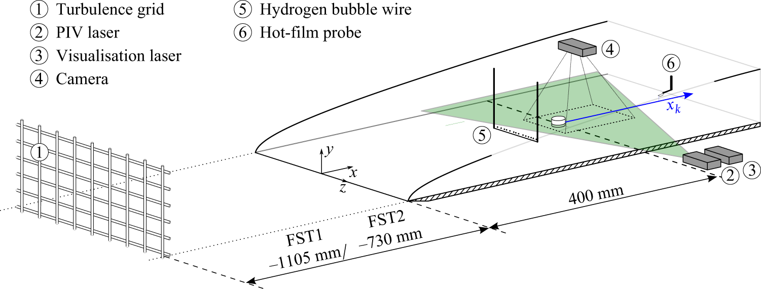
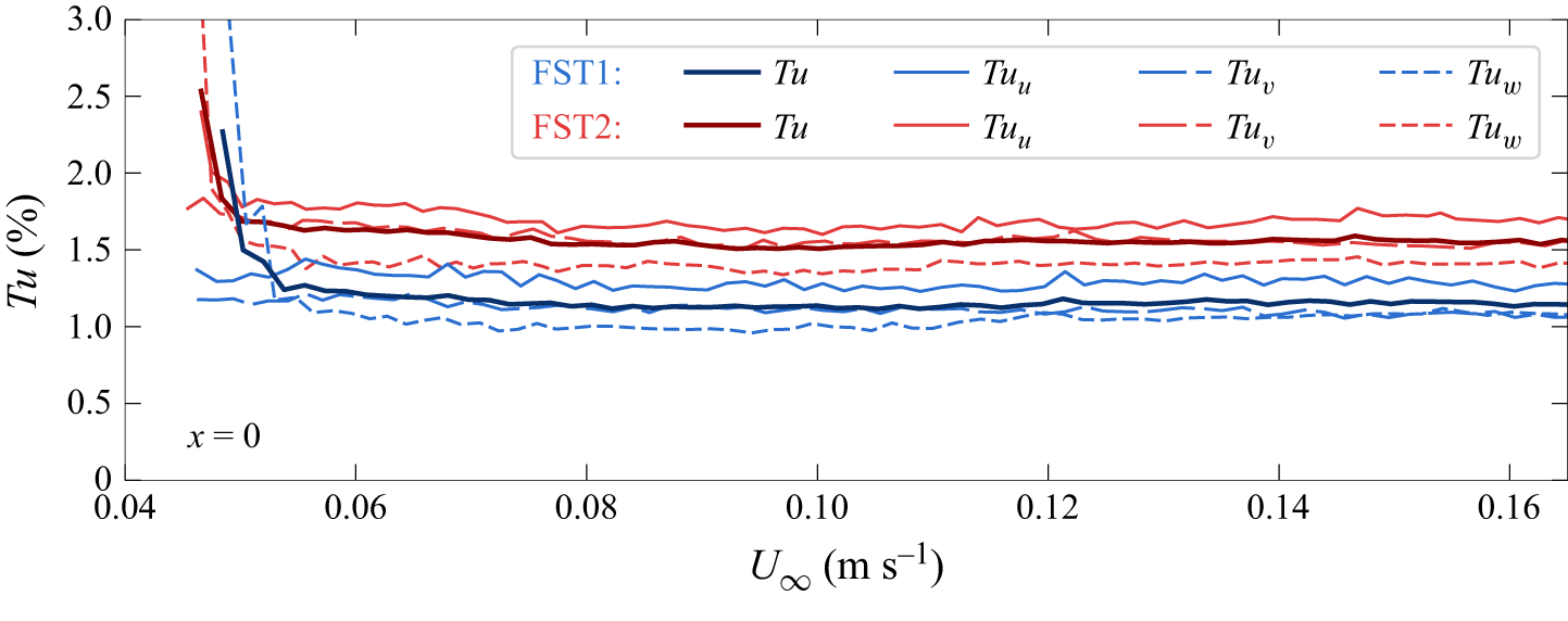


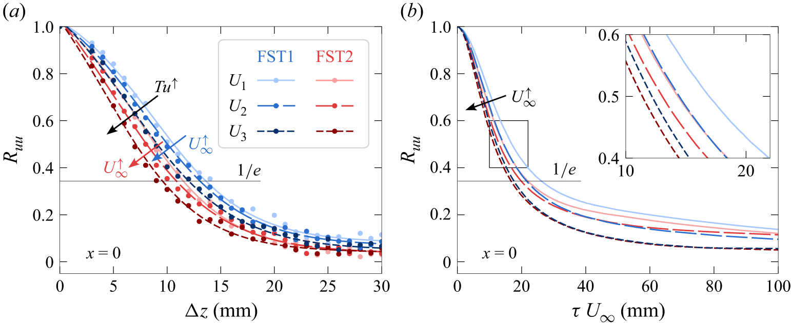


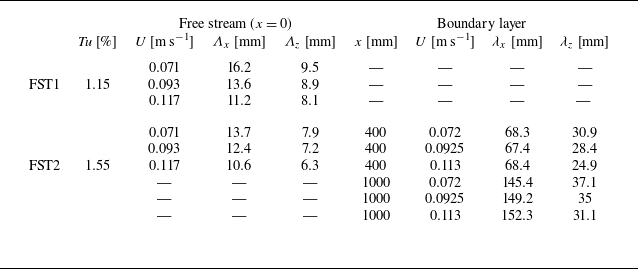


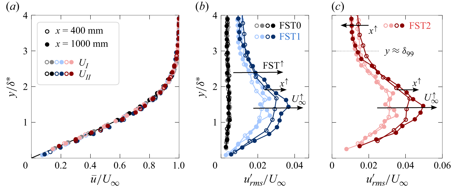


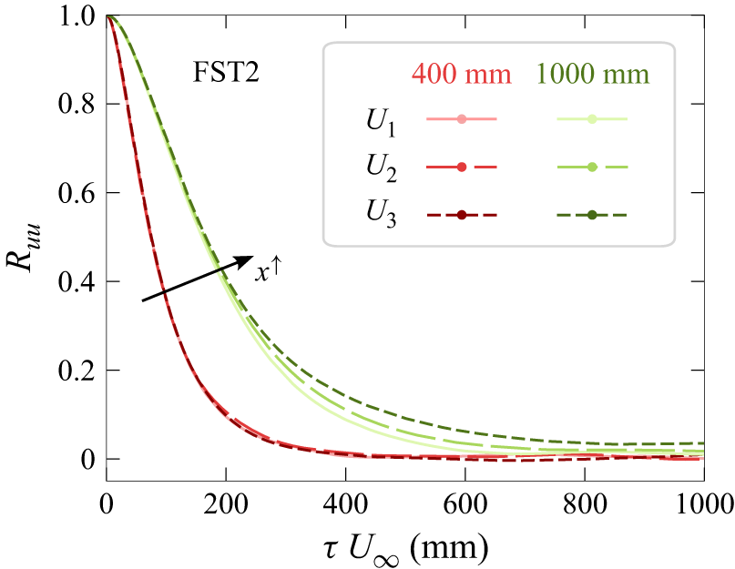

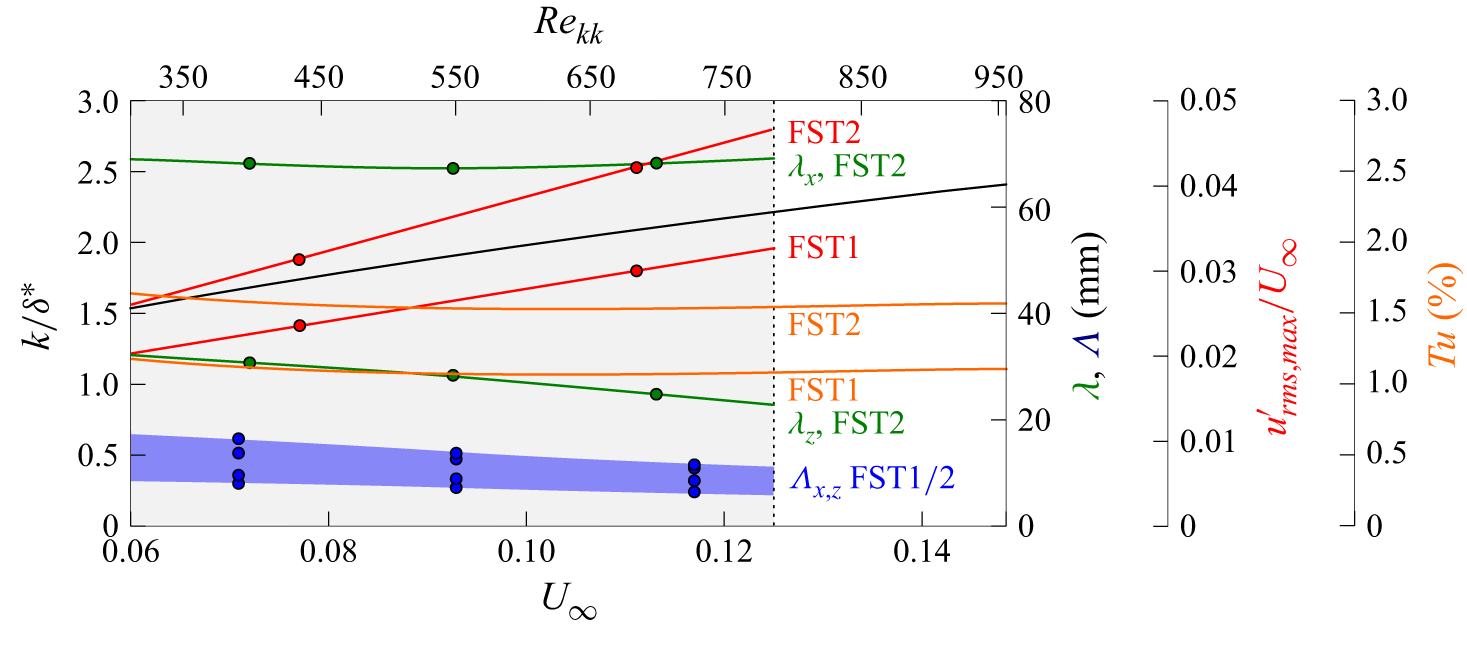


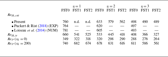


 Open access