





1. Introduction
A classic problem in fluid mechanics is the extraction of energy from a flow. Momentum theory for actuator strip (actuator disc theory) and the well-known Lanchester–Betz–Joukowsky limit (hereafter, the Betz limit) have provided a valuable guide to help engineers and scientists to analyse power generation for over a century. Fundamentally, the Betz limit represents an optimal balance between the thrust on the actuator disc and the velocity through it, assuming that the device power is a product of the thrust and the velocity. Actuator disc theory has been extended and refined in various ways. Whilst the analysis is general, the present work is primarily driven by questions that arise for tidal stream energy (Adcock et al. Reference Adcock, Draper, Willden and Vogel2021). Key developments of actuator disc theory in the context of tidal stream energy were the inclusion of blockage effects (Garrett & Cummins Reference Garrett and Cummins2007), the extension to two scales by Nishino & Willden (Reference Nishino and Willden2012b ) and further to an arbitrary number of scales by Dehtyriov et al. (Reference Dehtyriov, Schnabl, Vogel, Draper, Adcock and Willden2021).
The problem on which we focus in the present paper is how to arrange resistance across an actuator strip in a non-uniform flow where the flow is sheared in the vertical and/or horizontal plane. The general actuator strip could represent a single device or a co-planar array of devices (neglecting inter-turbine flows), with a spanwise-varying resistance distribution. Real tidal races have highly spatially variable energy density. This contrasts with the majority of the literature, which has considered scenarios where the incoming flow is uniform. For example, the analytical work on turbine arrangements, beyond that of Nishino & Willden (Reference Nishino and Willden2012b ), has focused on how to arrange rows of turbines in uniform flow (Draper & Nishino Reference Draper and Nishino2014). This has motivated the extension of classical actuator disc theory in a different direction to address this non-uniform flow problem.
A framework for the analysis of energy extraction in sheared flows was developed by Draper et al. (Reference Draper, Nishino, Adcock and Taylor2016). This framework assumed that the flow can be divided into multiple streamtubes that can be summed (or integrated) to solve for the fluid mechanics. To date, this has not been used to investigate how to optimise the distribution of resistance across the actuator strip. The present paper aims to address this gap. We also consider the related problem of the optimal resistance in a uniform flow, but one where the resistance may vary across the actuator strip, e.g. representing a non-uniform distribution of turbine resistance.
Beyond the analytical actuator disc approach, others have considered similar issues. Reviews of work on the performance of turbines in sheared flow are given in Vermeer, Sørensen & Crespo (Reference Vermeer, Sørensen and Crespo2003) and Sanderse, van der Pijl & Koren (Reference Sanderse, van der Pijl and Koren2011). Since it is difficult to generate controlled shear flow conditions without introducing turbulence in experiments and numerical simulations, many of these studies do not readily differentiate the effects of flow non-uniformity from other contributing factors in power generation. In the context of tidal power, various authors have investigated the optimal distribution of turbine properties within tidal arrays under uniform flow conditions (Hunter, Nishino & Willden Reference Hunter, Nishino and Willden2015; Bonar et al. Reference Bonar, Adcock, Venugopal and Borthwick2018). Extensions to non-uniform flows have also been explored, including through the use of sophisticated optimisation schemes (Funke et al. Reference Funke, Farrell and Piggott2014, Reference Funke, Kramer and Piggott2016). However, in these studies, the flow non-uniformity arises from the specified tidal channel geometry rather than being prescribed explicitly, making it difficult to isolate and interpret the influence of incoming flow non-uniformity on the optimisation results. These considerations motivate us to extend the theoretical framework of Draper et al. (Reference Draper, Nishino, Adcock and Taylor2016) to optimise the resistance distribution across an actuator disc strip in a prescribed non-uniform flow.
2. Methodology
2.1. Multi-streamtube theory
Following Draper et al. (Reference Draper, Nishino, Adcock and Taylor2016), we incorporate non-uniform resistance in the classical actuator disc theory by considering an actuator strip operating in a non-uniform flow in an infinitely wide channel. The velocity far upstream of the strip is $u(x_{1},z) \geqslant 0$
, and the coordinates are defined so that
$u(x_{1},z) \geqslant 0$
, and the coordinates are defined so that $x_{1}$
is a streamwise location far upstream of the strip, where the flow is undisturbed by the presence of the strip, and
$x_{1}$
is a streamwise location far upstream of the strip, where the flow is undisturbed by the presence of the strip, and $z$
is the spanwise coordinate at the actuator strip that takes zero value at the strip centre (see figure 1). Although
$z$
is the spanwise coordinate at the actuator strip that takes zero value at the strip centre (see figure 1). Although $z$
may represent either a cross-stream or a depth-wise coordinate, for simplicity it is taken here to be the cross-stream coordinate. As in the classical actuator disc analysis, we also assume that the flow is steady, incompressible and inviscid.
$z$
may represent either a cross-stream or a depth-wise coordinate, for simplicity it is taken here to be the cross-stream coordinate. As in the classical actuator disc analysis, we also assume that the flow is steady, incompressible and inviscid.
A non-uniform flow past an actuator strip.

To extract power, the strip must offer a resistance to the flow. Focusing on an infinitesimal control volume bounded by two neighbouring streamlines (or stream surfaces) and intersecting an area of strip $\delta l$
(per unit depth; see figure 1), we can introduce the resistance as a force
$\delta l$
(per unit depth; see figure 1), we can introduce the resistance as a force $\delta T$
on the fluid. Due to this force, fluid passing through the strip is reduced to a flow speed
$\delta T$
on the fluid. Due to this force, fluid passing through the strip is reduced to a flow speed $u(x_{2},z)=u_{2}(z)=\alpha _{2}(z)\,u_{1}(z)$
, where
$u(x_{2},z)=u_{2}(z)=\alpha _{2}(z)\,u_{1}(z)$
, where $\alpha _{2} \in [0, 1]$
and
$\alpha _{2} \in [0, 1]$
and $u_{1}(z)$
is the upstream velocity entering the control volume. Far downstream, the pressure is assumed to be constant for any
$u_{1}(z)$
is the upstream velocity entering the control volume. Far downstream, the pressure is assumed to be constant for any $z$
, and the velocity reduces further to
$z$
, and the velocity reduces further to $u(x_{4},z)=u_{4}(z)=\alpha _{4}(z)u_{1}(z)$
, where
$u(x_{4},z)=u_{4}(z)=\alpha _{4}(z)u_{1}(z)$
, where $\alpha _{4} \in [0, \alpha _{2}]$
. The flow passing through the entire actuator strip is obtained by integrating the flows through multiple infinitesimal streamtubes, which are assumed to be independent of one another (an assumption discussed further below).
$\alpha _{4} \in [0, \alpha _{2}]$
. The flow passing through the entire actuator strip is obtained by integrating the flows through multiple infinitesimal streamtubes, which are assumed to be independent of one another (an assumption discussed further below).
With this problem defined above, we can now relate the velocity coefficients within the control volume to the force applied by the strip, and in turn, the power removed by the strip. This analysis proceeds in the same way as in the classical actuator disc theory, except that we will focus here on the differential fluid element within the control volume rather than the whole strip. To do this, we apply mass conservation to deduce that
 \begin{equation} \delta l_{1}=\alpha _{2}(z)\,\delta l, \quad \delta l_{4}=\frac {\alpha _{2}(z)}{\alpha _{4}(z)}\,\delta l, \end{equation}
where $\delta l_{1}$
and
$\delta l_{1}$
and $\delta l_{4}$
define the widths of the control volume far upstream and far downstream of the strip, respectively. Next, assuming no other source of friction from
$\delta l_{4}$
define the widths of the control volume far upstream and far downstream of the strip, respectively. Next, assuming no other source of friction from $x_1$
to
$x_1$
to $x_4$
, we can apply the Bernoulli equation separately upstream and downstream of the strip to obtain an expression for the pressure difference across the strip:
$x_4$
, we can apply the Bernoulli equation separately upstream and downstream of the strip to obtain an expression for the pressure difference across the strip:
 \begin{equation} \Delta p= p(x_{2}, z)-p(x_{3}, z)=\frac {1}{2} \rho [u_{1}(z)]^{2} \left (1-[\alpha _{4}(z)]^{2}\right )\!, \end{equation}
where $x_{2}$
and
$x_{2}$
and $x_{3}$
are locations immediately upstream and downstream of the strip,
$x_{3}$
are locations immediately upstream and downstream of the strip, $p$
represents pressure, and
$p$
represents pressure, and $\rho$
is fluid density. Finally, to complete the analysis, conservation of streamwise momentum (for the control volume) leads to
$\rho$
is fluid density. Finally, to complete the analysis, conservation of streamwise momentum (for the control volume) leads to
 \begin{equation} \delta T = \rho\, u_{1}(z)\,\alpha _{2}(z)\,\delta l\, [\alpha _{4}(z) - 1]\,u_{1}(z) - \delta X, \end{equation}
where
 \begin{equation} \delta X = \oint _{\textit{CV}} p_x\, \text{d}s, \end{equation}
and $p_{x}$
is the streamwise component of pressure force acting normal to the surface of the control volume.
$p_{x}$
is the streamwise component of pressure force acting normal to the surface of the control volume.
Noting that $\Delta p=\delta T/\delta l$
, (2.1)–(2.3) can be combined to obtain a relationship between the velocity coefficient at the strip and the coefficient in the wake, which takes the form
$\Delta p=\delta T/\delta l$
, (2.1)–(2.3) can be combined to obtain a relationship between the velocity coefficient at the strip and the coefficient in the wake, which takes the form
 \begin{equation} \alpha _{2}(z) = \frac {1+\alpha _{4}(z)}{2}\left (1-\frac {\delta X}{\delta T}\right )\!. \end{equation}
The net resistance $\delta T/\delta l$
per unit width, or
$\delta T/\delta l$
per unit width, or $\Delta p$
, can be defined as
$\Delta p$
, can be defined as
 \begin{equation} \delta T/\delta l=\Delta p(z) = \frac {1}{2}\rho \,k(z)\,\bigl [u_{2}(z)\bigr ]^{2}, \end{equation}
where $k(z)$
is a local resistance coefficient for the actuator strip, which may vary across the actuator strip. The function
$k(z)$
is a local resistance coefficient for the actuator strip, which may vary across the actuator strip. The function $k(z)$
, defined along the spanwise location, can be interpreted as a non-dimensional measure of local resistance, with larger values of
$k(z)$
, defined along the spanwise location, can be interpreted as a non-dimensional measure of local resistance, with larger values of $k$
representing greater resistance.
$k$
representing greater resistance.
Combining (2.2), (2.5) and (2.6) yields
 \begin{equation} \alpha _2(z) = \frac {4}{k\big (z) + 4}. \end{equation}
Assuming $\delta X=0$
as in Draper et al. (Reference Draper, Nishino, Adcock and Taylor2016) (an assumption that we revisit below), and integrating across all streamtubes, the power removed by the entire strip (per unit depth) can be expressed as
$\delta X=0$
as in Draper et al. (Reference Draper, Nishino, Adcock and Taylor2016) (an assumption that we revisit below), and integrating across all streamtubes, the power removed by the entire strip (per unit depth) can be expressed as
 \begin{equation} P = \int _{-l/2}^{l/2} u_{2}(z)\,\Delta p(z)\,\text{d}z = \int _{-l_1/2}^{l_1/2} \alpha _{2}(z'(z))\,u_{1}(z'(z))\,\Delta p(z'(z))\,\text{d}z', \end{equation}
where
 \begin{align} l_{1} &= \int _{-l/2}^{l/2} \frac {4}{k(z)+4}\,\text{d}z,\\[-6pt]\nonumber \end{align}
 \begin{align} z'(z) &= \int _{0}^{z} \frac {4}{k(s) + 4} \, \text{d} s, \end{align}
in which $z'$
is the cross-stream coordinate of the streamtube upstream of the strip (figure 1). Equation (2.8) assumes that the flow is symmetric about
$z'$
is the cross-stream coordinate of the streamtube upstream of the strip (figure 1). Equation (2.8) assumes that the flow is symmetric about $z=0$
. Equation (2.9) is obtained by combining (2.1) and (2.7). Each streamtube is identified by its position
$z=0$
. Equation (2.9) is obtained by combining (2.1) and (2.7). Each streamtube is identified by its position $z$
at the strip, and maps to an upstream location
$z$
at the strip, and maps to an upstream location $z'$
at
$z'$
at $x_1$
. As the flow passes from
$x_1$
. As the flow passes from $x_1$
to
$x_1$
to $x_2$
(see figure 1), the streamtube width expands to satisfy mass conservation (2.1), with the expansion governed by the local resistance
$x_2$
(see figure 1), the streamtube width expands to satisfy mass conservation (2.1), with the expansion governed by the local resistance $k(z)$
based on (2.7). Combining (2.1) with (2.7), and integrating from the centreline to a general location
$k(z)$
based on (2.7). Combining (2.1) with (2.7), and integrating from the centreline to a general location $z$
, yields the mapping
$z$
, yields the mapping $z'(z)$
in (2.10), representing the cumulative streamtube expansion across the strip.
$z'(z)$
in (2.10), representing the cumulative streamtube expansion across the strip.
Presuming that the distribution of $\alpha _{2}(z)$
is known across the entire strip, (2.8) provides the general solution for the extracted power. Substituting (2.6) into (2.8) yields
$\alpha _{2}(z)$
is known across the entire strip, (2.8) provides the general solution for the extracted power. Substituting (2.6) into (2.8) yields
 \begin{equation} P = \int _{-l/2}^{\,l/2} \frac {1}{2}\rho \,k(z)\,\bigl [u_{2}(z)\bigr ]^{3}\text{d}z. \end{equation}
This integral (2.11) taken at the strip can be converted to an integral upstream of it:
 \begin{equation} P = \int _{-l_{1}/2}^{l_{1}/2} \frac {1}{2} \rho \, k\big (z'(z)\big ) \left ( \frac {4}{k\big (z'(z)\big ) + 4} \right )^{3} u_{1}\big (z'(z)\big )^{3} \text{d}z'. \end{equation}
When optimising the performance of an actuator strip for a given incoming flow velocity profile, it is reasonable to define a global power coefficient in the form
 \begin{equation} C_{\!p0} = \frac {P}{\frac {1}{2}\rho l\overline {U_0^{3}}}, \quad \text{with} \quad \overline {U_0^{3}} = \frac {1}{l}\int _{-l/2}^{l/2} \big[u_{1}\big(z'\big(z\big)\big)\big]^{3}\,\text{d}z'. \end{equation}
In this definition, the denominator is independent of $k(z/l)$
applied to the strip, such that maximising
$k(z/l)$
applied to the strip, such that maximising $C_{\!p0}$
is equivalent to maximising the extracted power. This power coefficient measures the global efficiency of energy extraction by the strip, and is consistent with the conventional formulation for a uniform incoming flow (Adcock et al. Reference Adcock, Draper, Willden and Vogel2021).
$C_{\!p0}$
is equivalent to maximising the extracted power. This power coefficient measures the global efficiency of energy extraction by the strip, and is consistent with the conventional formulation for a uniform incoming flow (Adcock et al. Reference Adcock, Draper, Willden and Vogel2021).
Alternatively, following Draper et al. (Reference Draper, Nishino, Adcock and Taylor2016), the power coefficient can be defined locally as
 \begin{equation} C_{\!p} = \frac {P}{\frac {1}{2}\rho l \overline {U^{3}}}, \quad \text{with} \quad \overline {U^{3}} = \frac {1}{l_{1}}\int _{-l_{1}/2}^{l_{1}/2} \big[u_{1}\big(z'\big(z\big)\big)\big]^{3}\,\text{d}z'. \end{equation}
The denominator of $C_p$
in (2.14) is defined such that in the case of a uniform resistance distribution, the dependence of the power coefficient on the strip resistance for non-uniform incoming flow is the same as that for conventional uniform flow, i.e.
$C_p$
in (2.14) is defined such that in the case of a uniform resistance distribution, the dependence of the power coefficient on the strip resistance for non-uniform incoming flow is the same as that for conventional uniform flow, i.e.
 \begin{equation} C_{\!p} = \frac {P}{\frac {1}{2}\rho l \overline {U^{3}}} = \frac {64k}{(k + 4)^{3}}, \end{equation}
which recovers the Betz limit when $k = 2$
. This power coefficient
$k = 2$
. This power coefficient $C_p$
measures a local efficiency of energy extraction at the strip, as it tracks the fluid passing through the strip. To maximise the power coefficient defined by (2.14), the resistance coefficient
$C_p$
measures a local efficiency of energy extraction at the strip, as it tracks the fluid passing through the strip. To maximise the power coefficient defined by (2.14), the resistance coefficient $k(z)$
should be optimised not only to maximise the integrand in the power expression (2.12), but also to ensure a significant collective width of the infinitesimal streamtubes, as described in (2.9).
$k(z)$
should be optimised not only to maximise the integrand in the power expression (2.12), but also to ensure a significant collective width of the infinitesimal streamtubes, as described in (2.9).
2.2. Optimisation methodology
Based on (2.13) and (2.14), the optimisation problem is formulated as
 \begin{equation} \begin{aligned} & \textit{max} \quad C_{\!p0}[ k(z);u_1(z)], \ C_p[ k(z);u_1(z)], \\ & \text{subject to}\quad k(z) \geqslant 0, \ u_1(z) \geqslant 0,\ z \in \left [-\frac {l}{2},\,\frac {l}{2}\right ]. \end{aligned} \end{equation}
The above problem is solved using the sequential quadratic programming algorithm implemented in MATLAB’s fmincon solver, with specified resistance distribution $k(z)$
and velocity distribution of incoming flow
$k(z)$
and velocity distribution of incoming flow $u_1(z)$
.
$u_1(z)$
.
2.3. Direct numerical simulations
Two-dimensional direct numerical simulations of the incompressible continuity and Navier–Stokes equations are solved:
 \begin{align} \boldsymbol{\nabla }\boldsymbol{\cdot }\boldsymbol{u} &= 0, \end{align}
 \begin{align} \frac {\partial \boldsymbol{u}}{\partial t} + \boldsymbol{u} \boldsymbol{\cdot }\boldsymbol{\nabla }\boldsymbol{u} &= -\frac {1}{\rho } \boldsymbol{\nabla }p + \nu\, {\nabla} ^{2} \boldsymbol{u} +\frac {\boldsymbol{f}}{\rho }, \end{align}
where $\mathit{{u}} = (u, v)(x, z, t)$
is the velocity vector,
$\mathit{{u}} = (u, v)(x, z, t)$
is the velocity vector, $t$
is time,
$t$
is time, $\nu$
is the kinematic viscosity, and
$\nu$
is the kinematic viscosity, and $\boldsymbol{f}$
is the external body force. Equations (2.17) and (2.18) were solved by using a spectral/hp element method embedded in the open-source software package Nektar
$\boldsymbol{f}$
is the external body force. Equations (2.17) and (2.18) were solved by using a spectral/hp element method embedded in the open-source software package Nektar $++$
(Cantwell et al. Reference Cantwell, Moxey, Comerford, Bolis, Rocco, Mengaldo, De Grazia, Yakovlev, Lombard and Ekelschot2015). A second-order time integration method was applied, together with a velocity correction scheme in the Galerkin formulation, as detailed in Blackburn & Sherwin (Reference Blackburn and Sherwin2004).
$++$
(Cantwell et al. Reference Cantwell, Moxey, Comerford, Bolis, Rocco, Mengaldo, De Grazia, Yakovlev, Lombard and Ekelschot2015). A second-order time integration method was applied, together with a velocity correction scheme in the Galerkin formulation, as detailed in Blackburn & Sherwin (Reference Blackburn and Sherwin2004).
A rectangular computational domain was used with streamwise dimension $80l$
and spanwise dimension
$80l$
and spanwise dimension $1000l$
. The centre of the actuator strip was placed at
$1000l$
. The centre of the actuator strip was placed at $x/l=0,\ z/l=0$
. The geometric blockage ratio is
$x/l=0,\ z/l=0$
. The geometric blockage ratio is $l/W=0.001$
, where
$l/W=0.001$
, where $l$
is the strip width, and
$l$
is the strip width, and $W$
is the channel width. Halving the geometric blockage ratio leads to minimal changes in the numerical results, suggesting negligible influence of spanwise boundaries. The strip Reynolds number varies from 100 to 10 000 (
$W$
is the channel width. Halving the geometric blockage ratio leads to minimal changes in the numerical results, suggesting negligible influence of spanwise boundaries. The strip Reynolds number varies from 100 to 10 000 ( $Re=U_{\infty }l/\nu$
).
$Re=U_{\infty }l/\nu$
).
A total of $N_c=153\,061$
macro-elements were used in the domain. Each macro-element was further subdivided using fourth-order Lagrange polynomials (denoted
$N_c=153\,061$
macro-elements were used in the domain. Each macro-element was further subdivided using fourth-order Lagrange polynomials (denoted $N_p = 4$
) for the quadrilateral expansions. The total number of mesh cells is
$N_p = 4$
) for the quadrilateral expansions. The total number of mesh cells is $(N_p -1)^2 \times N_c$
. A relatively high resolution was used in the region where body force was applied, with uniform cell size
$(N_p -1)^2 \times N_c$
. A relatively high resolution was used in the region where body force was applied, with uniform cell size $0.01l$
in the range
$0.01l$
in the range $x/l=[-1, 1]$
and
$x/l=[-1, 1]$
and $z/l=[-4, 4]$
. A mesh dependence study was performed, by varying
$z/l=[-4, 4]$
. A mesh dependence study was performed, by varying $N_p$
from 3 to 5. The relative differences in the spatial average of streamwise velocity
$N_p$
from 3 to 5. The relative differences in the spatial average of streamwise velocity $u_{2}(z)$
across the actuator strip, a key metric in this study, are within
$u_{2}(z)$
across the actuator strip, a key metric in this study, are within $0.1\,\%$
across this
$0.1\,\%$
across this $N_p$
range, which demonstrates the mesh convergence.
$N_p$
range, which demonstrates the mesh convergence.
A Dirichlet velocity boundary condition ( $u = U_{\infty }$
and
$u = U_{\infty }$
and $v = 0$
) was specified on the inlet (left-hand side of the computational domain) and spanwise boundaries, while on the outlet boundary (right-hand side of the domain), a Neumann velocity boundary condition (
$v = 0$
) was specified on the inlet (left-hand side of the computational domain) and spanwise boundaries, while on the outlet boundary (right-hand side of the domain), a Neumann velocity boundary condition ( $\partial u / \partial \boldsymbol{n} = 0$
and
$\partial u / \partial \boldsymbol{n} = 0$
and $\partial v / \partial \boldsymbol{n} = 0$
, where
$\partial v / \partial \boldsymbol{n} = 0$
, where $\boldsymbol{n}$
is the normal vector to the outlet boundary) was applied. The boundary conditions for the pressure included a reference value zero at the outlet, and a high-order Neumann condition following Karniadakis, Israeli & Orszag (Reference Karniadakis, Israeli and Orszag1991) at all other boundaries.
$\boldsymbol{n}$
is the normal vector to the outlet boundary) was applied. The boundary conditions for the pressure included a reference value zero at the outlet, and a high-order Neumann condition following Karniadakis, Israeli & Orszag (Reference Karniadakis, Israeli and Orszag1991) at all other boundaries.
Following Abedi & Eskilsson (Reference Abedi and Eskilsson2025), the actuator strip was represented by a spatially smooth, time-ramped resistance distribution per unit mass, applied explicitly to the momentum equation in the form of an acceleration ( $\boldsymbol{f}/\rho$
). The streamwise acceleration is then
$\boldsymbol{f}/\rho$
). The streamwise acceleration is then
 \begin{equation} f_x(x,z,t) = - \frac {1}{2} \, k(z) \, u^2 \, \mathcal{G}(x,z) \left [1 - \exp \left (-\frac {t}{\tau _{\mathit{ramp}}}\right )\right ]\!, \end{equation}
where $\tau _{\mathit{ramp}}=0.5$
is a ramping time introduced to prevent start-up transients. The spanwise distribution of the local resistance coefficient was prescribed as a specified function of
$\tau _{\mathit{ramp}}=0.5$
is a ramping time introduced to prevent start-up transients. The spanwise distribution of the local resistance coefficient was prescribed as a specified function of $z/l$
, where
$z/l$
, where $l = z_{\textit{max}} - z_{\textit{min}}$
. This distribution produces a smoothly varying load that vanishes at the edges of the strip.
$l = z_{\textit{max}} - z_{\textit{min}}$
. This distribution produces a smoothly varying load that vanishes at the edges of the strip.
The spatial distribution of the body force in the streamwise direction was modelled by a Gaussian kernel centred at $x = x_d = 0$
:
$x = x_d = 0$
:
 \begin{equation} \mathcal{G}(x,z) = \exp \!\left [-\frac {(x - x_d)^2}{\epsilon ^2}\right ] \left [ \frac {1}{2}\tanh \left (\frac {z - z_{\textit{min}}}{\delta l}\right ) - \frac {1}{2}\tanh \left (\frac {z - z_{\textit{max}}}{\delta l}\right ) \right ]\!, \end{equation}
where the Gaussian width was set to $\epsilon = 10^{-2}l$
, and
$\epsilon = 10^{-2}l$
, and $\delta =10^{-3}$
. With this set-up, the strip spans one
$\delta =10^{-3}$
. With this set-up, the strip spans one $p$
-type mesh cell in the streamwise direction. The kernel was normalised such that its area integral equals unity, with the normalisation constant
$p$
-type mesh cell in the streamwise direction. The kernel was normalised such that its area integral equals unity, with the normalisation constant $ {1}/({\epsilon \sqrt {\pi }\, l})$
.
$ {1}/({\epsilon \sqrt {\pi }\, l})$
.
3. Results
3.1. Optimisation with multi-streamtube theory
Using the optimisation algorithm, in this subsection, we present the optimised resistance distribution for both uniform and non-uniform incoming flows.
We start by considering simple linear variations in both the incoming flow and the resistance, as this captures the key fluid mechanics that we are exploring in a straightforward manner. The upstream velocity is defined by a piecewise linear function
 \begin{equation} u_1(z) = a_1 + a_2 \left | \frac {z}{l} \right |\! , \end{equation}
where $a_2\geqslant 0$
, indicating higher velocity towards the strip edge (
$a_2\geqslant 0$
, indicating higher velocity towards the strip edge ( $z/l \rightarrow \pm 0.5$
). To simplify the discussion, we hereafter assume
$z/l \rightarrow \pm 0.5$
). To simplify the discussion, we hereafter assume $a_1=1$
. Small values of
$a_1=1$
. Small values of $a_2$
may apply to a single turbine, whereas larger values of
$a_2$
may apply to a single turbine, whereas larger values of $a_2$
may represent a turbine array, since the effective shear perceived by the system is scale-dependent (see
$a_2$
may represent a turbine array, since the effective shear perceived by the system is scale-dependent (see $\S$
4.2 for details). The resistance coefficient across the strip is defined by a piecewise linear function as
$\S$
4.2 for details). The resistance coefficient across the strip is defined by a piecewise linear function as
 \begin{equation} k(z) = b_1 + b_2 \left |\frac {z}{l} \right |\!. \end{equation}
The optimisation results for $C_{\!p0}$
, presented in figure 2
$C_{\!p0}$
, presented in figure 2 $(a)$
, show that the optimal resistance distribution across the strip remains uniform (i.e.
$(a)$
, show that the optimal resistance distribution across the strip remains uniform (i.e. $b_1= 2$
,
$b_1= 2$
, $b_2= 0$
) regardless of the incoming flow profile. With increasing
$b_2= 0$
) regardless of the incoming flow profile. With increasing $a_2$
, the kinetic energy flux of the incoming flow in the denominator in the definition of
$a_2$
, the kinetic energy flux of the incoming flow in the denominator in the definition of $C_{\!p0}$
in (2.13) increases, while the extracted power (i.e. the numerator in (2.13)) remains equal to that corresponding to the Betz limit. This results in a decreased
$C_{\!p0}$
in (2.13) increases, while the extracted power (i.e. the numerator in (2.13)) remains equal to that corresponding to the Betz limit. This results in a decreased $C_{\!p0}$
value in figure 2
$C_{\!p0}$
value in figure 2 $(b)$
. Fundamentally, maximising
$(b)$
. Fundamentally, maximising $C_{\!p0}$
is equivalent to maximising the integral of power over all streamtubes in (2.12), which is also equivalent to maximising the power extracted from each individual streamtube. For a given streamtube, both the incoming flow and the resistance distribution can be assumed to be uniform, for which the power coefficient is maximised at the well-known
$C_{\!p0}$
is equivalent to maximising the integral of power over all streamtubes in (2.12), which is also equivalent to maximising the power extracted from each individual streamtube. For a given streamtube, both the incoming flow and the resistance distribution can be assumed to be uniform, for which the power coefficient is maximised at the well-known $k=2$
. This is the reason why a constant optimal
$k=2$
. This is the reason why a constant optimal $k(z/l)=2$
is seen across the actuator strip in figure 2
$k(z/l)=2$
is seen across the actuator strip in figure 2 $(c)$
.
$(c)$
.
Optimised piecewise linear resistance distribution of (3.2) for piecewise linear velocity profile (3.1) with $a_2\geqslant 0$
, maximising
$a_2\geqslant 0$
, maximising $C_{\!p0}$
. (
$C_{\!p0}$
. ( $a$
) The variation of optimal values of
$a$
) The variation of optimal values of $b_{1}$
and
$b_{1}$
and $b_{2}$
with
$b_{2}$
with $a_2$
. (
$a_2$
. ( $b$
) The variation of the power coefficient with
$b$
) The variation of the power coefficient with $a_2$
. (
$a_2$
. ( $c$
) Resistance coefficient profile for selected values of
$c$
) Resistance coefficient profile for selected values of $a_2$
.
$a_2$
.

In contrast with $C_{\!p0}$
, the optimisation results for
$C_{\!p0}$
, the optimisation results for $C_p$
in figure 3 demonstrate that the optimal resistance distributions (given the constraints of (3.2)) across the strip are uniform and non-uniform for uniform and non-uniform flows, respectively. First, for
$C_p$
in figure 3 demonstrate that the optimal resistance distributions (given the constraints of (3.2)) across the strip are uniform and non-uniform for uniform and non-uniform flows, respectively. First, for $a_2 = 0$
(i.e. uniform flow),
$a_2 = 0$
(i.e. uniform flow), $b_1 = 2$
and
$b_1 = 2$
and $b_2 = 0$
, which is consistent with the conventional optimal constant local resistance coefficient 2 (see figure 3
$b_2 = 0$
, which is consistent with the conventional optimal constant local resistance coefficient 2 (see figure 3 $a$
). This resistance distribution gives the classical Betz limit
$a$
). This resistance distribution gives the classical Betz limit $C_{\!p} = 16/27$
(figure 3
$C_{\!p} = 16/27$
(figure 3 $b$
). As soon as the incoming flow becomes non-uniform (i.e.
$b$
). As soon as the incoming flow becomes non-uniform (i.e. $a_2\gt 0$
), the optimal distribution of resistance across the strip becomes also non-uniform as
$a_2\gt 0$
), the optimal distribution of resistance across the strip becomes also non-uniform as $b_2\gt 0$
(see figure 3
$b_2\gt 0$
(see figure 3 $a$
). While the value of
$a$
). While the value of $b_1$
decreases with
$b_1$
decreases with $a_2$
, the
$a_2$
, the $b_2$
value increases (figure 3
$b_2$
value increases (figure 3 $a$
). Physically, when the
$a$
). Physically, when the $a_2$
value increases, the flow becomes more sheared, with higher velocity approaching either side of the strip relative to that towards the strip centre. In response to this, more resistance should be placed in the high-velocity region to achieve the optimal strip performance. It is seen from figure 3(
$a_2$
value increases, the flow becomes more sheared, with higher velocity approaching either side of the strip relative to that towards the strip centre. In response to this, more resistance should be placed in the high-velocity region to achieve the optimal strip performance. It is seen from figure 3( $b$
) that the optimised power coefficient increases with
$b$
) that the optimised power coefficient increases with $a_2$
. Given the chosen normalisation of the power coefficient, the more sheared the flow is, the higher the potential of an actuator strip.
$a_2$
. Given the chosen normalisation of the power coefficient, the more sheared the flow is, the higher the potential of an actuator strip.
Optimised piecewise linear resistance distribution of (3.2) for piecewise linear velocity profile (3.1) with $a_2\geqslant 0$
, maximising
$a_2\geqslant 0$
, maximising $C_{\!p}$
. (
$C_{\!p}$
. ( $a$
) The variation of optimal values of
$a$
) The variation of optimal values of $b_{1}$
and
$b_{1}$
and $b_{2}$
with
$b_{2}$
with $a_2$
. (
$a_2$
. ( $b$
) The variation of the power coefficient with
$b$
) The variation of the power coefficient with $a_2$
. (
$a_2$
. ( $c$
) Resistance coefficient profile for selected values of
$c$
) Resistance coefficient profile for selected values of $a_2$
.
$a_2$
.

The resistance distribution profile is presented for selected values of $a_2$
in figure 3(
$a_2$
in figure 3( $c$
). With increasing
$c$
). With increasing $a_2$
, the
$a_2$
, the $k$
value increases at the two strip edges, but decreases at the strip centre. All the profiles intersect at
$k$
value increases at the two strip edges, but decreases at the strip centre. All the profiles intersect at $|z/l|\approx 0.3$
. It is noted that the lateral expansion rate of a streamtube from
$|z/l|\approx 0.3$
. It is noted that the lateral expansion rate of a streamtube from $x_1$
to
$x_1$
to $x_2$
is proportional to local
$x_2$
is proportional to local $k(z/l)$
according to (2.1) and (2.7). With this in mind, if one assumes that all individual streamtubes have the same width at the upstream location
$k(z/l)$
according to (2.1) and (2.7). With this in mind, if one assumes that all individual streamtubes have the same width at the upstream location $x_1$
, then figure 3(
$x_1$
, then figure 3( $c$
) shows that it is better for some streamtubes (in faster flowing areas) to have a higher than optimal (
$c$
) shows that it is better for some streamtubes (in faster flowing areas) to have a higher than optimal ( $k=2$
) local value so that they occupy more area within the strip at
$k=2$
) local value so that they occupy more area within the strip at $x_2$
and remove more power from the flow. In slower-flowing regions, the opposite is true: streamtubes have a local
$x_2$
and remove more power from the flow. In slower-flowing regions, the opposite is true: streamtubes have a local $k(z/l)$
smaller than the optimum
$k(z/l)$
smaller than the optimum $k=2$
, and therefore occupy a relatively smaller portion of the strip area.
$k=2$
, and therefore occupy a relatively smaller portion of the strip area.
The optimal resistance distribution depends on the distribution function applied across the strip for a given non-uniform flow. For example, for the same velocity profile of incoming flow defined by (3.1), in maximising $C_p$
, figure 4 presents the variation of the optimal values of resistance parameters
$C_p$
, figure 4 presents the variation of the optimal values of resistance parameters $b_1$
and
$b_1$
and $b_2$
with
$b_2$
with $a_2$
for a different parabolic function, defined as
$a_2$
for a different parabolic function, defined as
 \begin{equation} k(z) = b_1 + b_2 \left ( \frac {z}{l} \right )^2\!. \end{equation}
For this new function, the variation trend of $b_1$
and
$b_1$
and $b_2$
with
$b_2$
with $a_2$
is similar to that for the piecewise linear function described above (comparing figures 4(a) and 3(a)). The resistance profiles also intersect approximately at
$a_2$
is similar to that for the piecewise linear function described above (comparing figures 4(a) and 3(a)). The resistance profiles also intersect approximately at $|z/l|=0.3$
(figure 4
$|z/l|=0.3$
(figure 4 $c$
). However, for a given value of
$c$
). However, for a given value of $a_2$
, the power coefficient for the parabolic function is lower than that for the piecewise linear function. This suggests that it is better to match the resistance distribution function to the velocity profile of incoming flow in the optimisation. This observation is confirmed by examining another mismatched case, considering a parabolic velocity profile
$a_2$
, the power coefficient for the parabolic function is lower than that for the piecewise linear function. This suggests that it is better to match the resistance distribution function to the velocity profile of incoming flow in the optimisation. This observation is confirmed by examining another mismatched case, considering a parabolic velocity profile $u_1(z)=a_1+a_2(z/l)^2$
(assuming
$u_1(z)=a_1+a_2(z/l)^2$
(assuming $a_1=1$
) combined with a piecewise linear resistance distribution defined by (3.2). For the same values of
$a_1=1$
) combined with a piecewise linear resistance distribution defined by (3.2). For the same values of $a_2$
, the resulting
$a_2$
, the resulting $C_p$
(not shown) is even lower than that obtained from the combinations of (3.1) with (3.2) or (3.1) with (3.3). Nevertheless, figures 4 and 3 as a combination highlight the potential of maximising the power extraction efficiency of the strip by tuning the resistance distribution across the strip for a non-uniform flow.
$C_p$
(not shown) is even lower than that obtained from the combinations of (3.1) with (3.2) or (3.1) with (3.3). Nevertheless, figures 4 and 3 as a combination highlight the potential of maximising the power extraction efficiency of the strip by tuning the resistance distribution across the strip for a non-uniform flow.
Optimised parabolic resistance distribution of (3.3) for velocity profile (3.1) with $a_2\geqslant 0$
, maximising
$a_2\geqslant 0$
, maximising $C_{\!p}$
. (
$C_{\!p}$
. ( $a$
) The variation of optimal values of
$a$
) The variation of optimal values of $b_{1}$
and
$b_{1}$
and $b_{2}$
with
$b_{2}$
with $a_2$
. (
$a_2$
. ( $b$
) The variation of the power coefficient with
$b$
) The variation of the power coefficient with $a_2$
. (
$a_2$
. ( $c$
) Resistance coefficient profile for selected values of
$c$
) Resistance coefficient profile for selected values of $a_2$
.
$a_2$
.

There is also a dependency of optimal resistance distribution on the velocity profile of incoming flow for maximising $C_p$
. This can be demonstrated by changing
$C_p$
. This can be demonstrated by changing $a_2$
in (3.1) to negative values (
$a_2$
in (3.1) to negative values ( $a_2\leqslant 0$
), for which the velocity decreases towards the edge from the strip centre. By assuming a piecewise linear function for the resistance distribution as described by (3.2), figure 5 shows an opposite resistance distribution across the strip, compared to that for
$a_2\leqslant 0$
), for which the velocity decreases towards the edge from the strip centre. By assuming a piecewise linear function for the resistance distribution as described by (3.2), figure 5 shows an opposite resistance distribution across the strip, compared to that for $a_2\geqslant 0$
shown in figure 3. Again, it is shown in figure 5 that higher resistance should be placed in the high-velocity regions. With decreasing
$a_2\geqslant 0$
shown in figure 3. Again, it is shown in figure 5 that higher resistance should be placed in the high-velocity regions. With decreasing $a_2$
, the value of
$a_2$
, the value of $b_2$
initially decreases rapidly, together with an increase of
$b_2$
initially decreases rapidly, together with an increase of $b_1$
. Once the
$b_1$
. Once the $k$
value reaches zero at the strip edge,
$k$
value reaches zero at the strip edge, $b_2$
increases slightly with decreasing
$b_2$
increases slightly with decreasing $a_2$
, due to the imposed non-negative
$a_2$
, due to the imposed non-negative $k$
constraints in the optimisation process. This leads to the formation of a kink at
$k$
constraints in the optimisation process. This leads to the formation of a kink at $a_2=-1.34$
in figure 5
$a_2=-1.34$
in figure 5 $(a)$
. For the same absolute value
$(a)$
. For the same absolute value $|a_2|=2$
, the optimal power coefficient for the velocity profile with
$|a_2|=2$
, the optimal power coefficient for the velocity profile with $a_2=-2$
exceeds 0.68 (figure 5
$a_2=-2$
exceeds 0.68 (figure 5 $b$
), which is much larger than that for
$b$
), which is much larger than that for $a_2=2$
(figure 3
$a_2=2$
(figure 3 $b$
).
$b$
).
Optimised piecewise linear resistance distribution of (3.2) for velocity profile (3.1) with $a_2\leqslant 0$
, maximising
$a_2\leqslant 0$
, maximising $C_{\!p}$
. (
$C_{\!p}$
. ( $a$
) The variation of optimal values of
$a$
) The variation of optimal values of $b_{1}$
and
$b_{1}$
and $b_{2}$
with
$b_{2}$
with $a_2$
, with a kink at
$a_2$
, with a kink at $a_2= -1.34$
. (
$a_2= -1.34$
. ( $b$
) The variation of the power coefficient with
$b$
) The variation of the power coefficient with $a_2$
. (
$a_2$
. ( $c$
) Resistance coefficient profile for selected values of
$c$
) Resistance coefficient profile for selected values of $a_2$
.
$a_2$
.

The curve in figure 5 $(b)$
has the same form as that in figure 3
$(b)$
has the same form as that in figure 3 $(b)$
, but varies in the opposite direction of
$(b)$
, but varies in the opposite direction of $a_2$
. The case with
$a_2$
. The case with $a_2= 2$
in figure 3
$a_2= 2$
in figure 3 $(b)$
, for example, produces a velocity profile in which the maximum value is twice as large as the minimum. In figure 5
$(b)$
, for example, produces a velocity profile in which the maximum value is twice as large as the minimum. In figure 5 $(b)$
,
$(b)$
, $-a_2= 1$
yields the same result and therefore the same maximised
$-a_2= 1$
yields the same result and therefore the same maximised $C_p$
value. These results are identical because mathematically, the streamtubes do not know where they are on the strip, and they only ‘feel’ the constraint that the sum of the streamtube widths at the strip location
$C_p$
value. These results are identical because mathematically, the streamtubes do not know where they are on the strip, and they only ‘feel’ the constraint that the sum of the streamtube widths at the strip location $x_2$
must equal the total strip width
$x_2$
must equal the total strip width $l$
. In other words, optimising
$l$
. In other words, optimising $C_p$
for the streamtubes at
$C_p$
for the streamtubes at $a_2 = 2$
is equivalent to that at
$a_2 = 2$
is equivalent to that at $a_2 = -1$
, since the streamtubes across the strip are independent of the direction of the shear and depend only on the shear magnitude.
$a_2 = -1$
, since the streamtubes across the strip are independent of the direction of the shear and depend only on the shear magnitude.
Figure 6 demonstrates that the ratio $|b_2/b_1|$
varies differently with
$|b_2/b_1|$
varies differently with $|a_2|$
for different velocity profiles of incoming flow and resistance distribution across the strip. For the parabolic incoming flow profile and piecewise linear resistance distribution (red dashed line), the optimal ratio
$|a_2|$
for different velocity profiles of incoming flow and resistance distribution across the strip. For the parabolic incoming flow profile and piecewise linear resistance distribution (red dashed line), the optimal ratio $|b_2/b_1|$
scales linearly with
$|b_2/b_1|$
scales linearly with $|a_2|$
. In contrast, for the same resistance distribution but with the piecewise linear incoming flow profile (
$|a_2|$
. In contrast, for the same resistance distribution but with the piecewise linear incoming flow profile ( $a_2\geqslant 0$
) (black solid line), the optimal ratio
$a_2\geqslant 0$
) (black solid line), the optimal ratio $|b_2/b_1|$
exhibits scaling factor approximately 2.5 with respect to
$|b_2/b_1|$
exhibits scaling factor approximately 2.5 with respect to $|a_2|$
. For the same linear incoming flow profile with
$|a_2|$
. For the same linear incoming flow profile with $a_2\geqslant 0$
(comparing black solid and dot-dashed lines), it is more efficient to optimise the resistance following a parabolic function compared to a piecewise linear function, as indicated by larger scaling factor between
$a_2\geqslant 0$
(comparing black solid and dot-dashed lines), it is more efficient to optimise the resistance following a parabolic function compared to a piecewise linear function, as indicated by larger scaling factor between $|b_2/b_1|$
and
$|b_2/b_1|$
and $|a_2|$
.
$|a_2|$
.
Comparison of optimal $b_2/b_1$
against
$b_2/b_1$
against $|a_2|$
for maximising
$|a_2|$
for maximising $C_p$
for different incoming flow profiles and resistance distributions.
$C_p$
for different incoming flow profiles and resistance distributions.

3.2. Numerical results
Figures 2( $a$
) and 3(
$a$
) and 3( $a$
) in combination demonstrate that the analytical optimal resistance is uniform for a uniform incoming flow regardless of the power coefficient definition, and is consistent with findings from numerical simulations (Hunter et al. Reference Hunter, Nishino and Willden2015; Bonar et al. Reference Bonar, Adcock, Venugopal and Borthwick2018). Fundamentally, for a uniform incoming flow, optimising the resistance distribution across the actuator strip through the multi-streamtube theory is equivalent to optimising the resistance for any streamtube due to the uniformity of the incoming flow. However, the optimal constant local resistance coefficient 2 may be large enough to cause significant flow diversion around the strip, leading to cross-stream variation in the local flow field, with higher velocities towards the strip edges (Nishino & Willden Reference Nishino and Willden2012a
; He et al. Reference He, Draper, Ghisalberti, An and Branson2024). This result implies that
$a$
) in combination demonstrate that the analytical optimal resistance is uniform for a uniform incoming flow regardless of the power coefficient definition, and is consistent with findings from numerical simulations (Hunter et al. Reference Hunter, Nishino and Willden2015; Bonar et al. Reference Bonar, Adcock, Venugopal and Borthwick2018). Fundamentally, for a uniform incoming flow, optimising the resistance distribution across the actuator strip through the multi-streamtube theory is equivalent to optimising the resistance for any streamtube due to the uniformity of the incoming flow. However, the optimal constant local resistance coefficient 2 may be large enough to cause significant flow diversion around the strip, leading to cross-stream variation in the local flow field, with higher velocities towards the strip edges (Nishino & Willden Reference Nishino and Willden2012a
; He et al. Reference He, Draper, Ghisalberti, An and Branson2024). This result implies that $\delta X$
defined in (2.4) is not exact. Therefore, although the flow is uniform far upstream of the strip, the flow can be locally non-uniform around the strip. This physics is not captured with multi-streamtube theory. Nevertheless, we may use the analytical results for non-uniform flow to suggest that once the flow becomes non-uniform, it may be possible to improve the performance by tuning the resistance distribution to match the local non-uniform flow. This motivates us to conduct direct numerical simulations of uniform flow past an actuator strip to check if the local flow field is two-dimensional, and if so, then to further optimise the resistance with considering the local variability in the flow.
$\delta X$
defined in (2.4) is not exact. Therefore, although the flow is uniform far upstream of the strip, the flow can be locally non-uniform around the strip. This physics is not captured with multi-streamtube theory. Nevertheless, we may use the analytical results for non-uniform flow to suggest that once the flow becomes non-uniform, it may be possible to improve the performance by tuning the resistance distribution to match the local non-uniform flow. This motivates us to conduct direct numerical simulations of uniform flow past an actuator strip to check if the local flow field is two-dimensional, and if so, then to further optimise the resistance with considering the local variability in the flow.
Figure 7 presents the time mean field of streamwise velocity for flow past an actuator strip with constant $k(z/l)=2$
across the strip, demonstrating the two-dimensionality of the local flow. It is seen that in the centre region of the strip, the streamwise velocity is virtually uniform. However, towards either strip edge (
$k(z/l)=2$
across the strip, demonstrating the two-dimensionality of the local flow. It is seen that in the centre region of the strip, the streamwise velocity is virtually uniform. However, towards either strip edge ( $z/l \rightarrow \pm 0.5$
), the streamlines are diverging, indicating two-dimensionality, which is consistent with that described by Nishino & Willden (Reference Nishino and Willden2012a
). This suggests the possibility of optimising strip performance by considering local flow variability.
$z/l \rightarrow \pm 0.5$
), the streamlines are diverging, indicating two-dimensionality, which is consistent with that described by Nishino & Willden (Reference Nishino and Willden2012a
). This suggests the possibility of optimising strip performance by considering local flow variability.
Time mean field of streamwise velocity for uniform incoming flow past a porous strip with constant $k(z/l)=2$
and
$k(z/l)=2$
and $Re=100$
.
$Re=100$
.

Figure 8 shows the variation of power coefficient $C_{\!p}$
with parameter
$C_{\!p}$
with parameter $b_{2}$
, in which results from numerical simulations and predictions using multi-streamtube theory are compared. In this plot, the resistance across the strip is assumed to follow the parabolic function defined by (3.3) while maintaining the spatial average of
$b_{2}$
, in which results from numerical simulations and predictions using multi-streamtube theory are compared. In this plot, the resistance across the strip is assumed to follow the parabolic function defined by (3.3) while maintaining the spatial average of $k(z/l)$
across the strip being constant at 2. Overall, with increasing
$k(z/l)$
across the strip being constant at 2. Overall, with increasing $b_{2}$
from
$b_{2}$
from $-12$
to 24, the power coefficient first increases and then decreases for both numerical and analytical results. The numerical values of
$-12$
to 24, the power coefficient first increases and then decreases for both numerical and analytical results. The numerical values of $C_{\!p}$
are larger than theoretical predictions across the full range of
$C_{\!p}$
are larger than theoretical predictions across the full range of $b_{2}$
, and the difference between them increases with
$b_{2}$
, and the difference between them increases with $b_{2}$
. This confirms a higher
$b_{2}$
. This confirms a higher $C_{\!p}$
value from the numerical simulation than that predicted by classical actuator disc theory for a uniform resistance distribution with
$C_{\!p}$
value from the numerical simulation than that predicted by classical actuator disc theory for a uniform resistance distribution with $k=2$
, i.e.
$k=2$
, i.e. $b_2=0$
as reported by Belloni (Reference Belloni2013).
$b_2=0$
as reported by Belloni (Reference Belloni2013).


A key finding in figure 8 is that while the analytically predicted power coefficient peaks at $b_{2}=0$
with the classical Betz limit 0.59, the numerical
$b_{2}=0$
with the classical Betz limit 0.59, the numerical $C_p$
value continues to increase with increasing
$C_p$
value continues to increase with increasing $b_2$
from
$b_2$
from $-12$
, before reaching peak value
$-12$
, before reaching peak value $C_{\!p}= 0.67$
at
$C_{\!p}= 0.67$
at $b_{2}= 4.8$
(
$b_{2}= 4.8$
( $b_{1}=1.6$
). Importantly, this is a
$b_{1}=1.6$
). Importantly, this is a $C_p$
value higher than the classical Betz limit, and it arises from a non-uniform distribution of
$C_p$
value higher than the classical Betz limit, and it arises from a non-uniform distribution of $k$
across the strip. In the increase of
$k$
across the strip. In the increase of $b_2$
from
$b_2$
from $-12$
to 4.8, the resistance distribution varies from a convex to a concave parabola (as sketched in figure 8), matching better the variation of streamwise velocity across the strip that is higher towards the strip edge (as shown in figure 7). This confirms the hypothesis that it is possible to tune the local resistance distribution to match the local flow variability to optimise the strip performance.
$-12$
to 4.8, the resistance distribution varies from a convex to a concave parabola (as sketched in figure 8), matching better the variation of streamwise velocity across the strip that is higher towards the strip edge (as shown in figure 7). This confirms the hypothesis that it is possible to tune the local resistance distribution to match the local flow variability to optimise the strip performance.
The difference in the power coefficient $C_p$
between the realistic numerical model, which incorporates viscous effects, and the idealised analytical model, which assumes inviscid flow, decreases as the Reynolds number increases. Figure 8 shows that as the Reynolds number increases from 100 to 500, the power coefficient decreases for all values of
$C_p$
between the realistic numerical model, which incorporates viscous effects, and the idealised analytical model, which assumes inviscid flow, decreases as the Reynolds number increases. Figure 8 shows that as the Reynolds number increases from 100 to 500, the power coefficient decreases for all values of $b_2$
. A smaller reduction in
$b_2$
. A smaller reduction in $C_p$
is observed as the Reynolds number increases from 500 through 1000 to 10 000, suggesting convergence of the results for
$C_p$
is observed as the Reynolds number increases from 500 through 1000 to 10 000, suggesting convergence of the results for $Re \gtrsim 1000$
. Nevertheless, the variations in
$Re \gtrsim 1000$
. Nevertheless, the variations in $C_p$
obtained from the numerical simulations follow a similar trend with respect to
$C_p$
obtained from the numerical simulations follow a similar trend with respect to $b_2$
, demonstrating the potential for optimising the resistance distribution while accounting for local flow variability.
$b_2$
, demonstrating the potential for optimising the resistance distribution while accounting for local flow variability.
While the numerical simulations show power coefficients exceeding the classical Betz limit in figure 8 for a uniform incoming flow, the observed increase in $C_p$
does not constitute a violation of this fundamental limit. The Betz limit is derived under the assumptions of uniform, inviscid flow within a one-dimensional momentum framework. In contrast, the present numerical study involves spatially varying resistance, along with additional effects such as flow diversion and viscosity. As a result, the classical assumptions underlying the Betz limit are not satisfied in this configuration. Therefore, the observed increase in
$C_p$
does not constitute a violation of this fundamental limit. The Betz limit is derived under the assumptions of uniform, inviscid flow within a one-dimensional momentum framework. In contrast, the present numerical study involves spatially varying resistance, along with additional effects such as flow diversion and viscosity. As a result, the classical assumptions underlying the Betz limit are not satisfied in this configuration. Therefore, the observed increase in $C_p$
reflects the specific flow conditions and the turbine representation employed, rather than a breach of the classical theoretical limit.
$C_p$
reflects the specific flow conditions and the turbine representation employed, rather than a breach of the classical theoretical limit.
The difference in the power coefficient $C_{\!p}$
between numerical simulations and theoretical predictions in figure 8 can be explained by comparing the cross-stream profile of streamwise velocity and the local power coefficient
$C_{\!p}$
between numerical simulations and theoretical predictions in figure 8 can be explained by comparing the cross-stream profile of streamwise velocity and the local power coefficient $C_{\!p}^{\prime}$
for different resistance distributions in figure 9. The local power coefficient is defined as
$C_{\!p}^{\prime}$
for different resistance distributions in figure 9. The local power coefficient is defined as
 \begin{equation} C_{\!p}^{\prime} = \frac {\frac {1}{2}\rho \, k(z)\,\delta l\,[u_2(z)]^3}{\frac {1}{2}\rho \, \delta l\,[u_1(z)]^3} = \frac {k(z)\,[u_2(z)]^3}{[u_1(z)]^3}. \end{equation}
(a,d,g) Distribution of resistance coefficient assumed in numerical simulations and theory. $(b, e, h)$
Comparison of cross-stream profiles of streamwise velocity at
$(b, e, h)$
Comparison of cross-stream profiles of streamwise velocity at $x/l=0$
between numerical simulations and predictions using multi-streamtube theory.
$x/l=0$
between numerical simulations and predictions using multi-streamtube theory. $(c, f, i)$
Comparison of cross-stream profiles of local power coefficient at
$(c, f, i)$
Comparison of cross-stream profiles of local power coefficient at $x/l=0$
between numerical simulations and predictions. The strip spans
$x/l=0$
between numerical simulations and predictions. The strip spans $z/l=[-0.5, 0.5]$
and
$z/l=[-0.5, 0.5]$
and $Re=100$
. While
$Re=100$
. While $b_1=2, b_2=0$
for
$b_1=2, b_2=0$
for $(a, b,c)$
,
$(a, b,c)$
, $b_1=3, b_2=-12$
for
$b_1=3, b_2=-12$
for $(d,e,f)$
, and
$(d,e,f)$
, and $b_1=1.6, b_2=4.8$
for
$b_1=1.6, b_2=4.8$
for $(g,h,i)$
, the spatial average of
$(g,h,i)$
, the spatial average of $k$
across the strip remains 2.
$k$
across the strip remains 2.

Overall, for all the three representative resistance distributions (figures 9
a,d,g), the measured velocities across the strip ( $-0.5\leqslant z/l\leqslant 0.5$
) are higher than those predicted in figures 9(b), 9(e) and 9(h). As a result, the numerical values of
$-0.5\leqslant z/l\leqslant 0.5$
) are higher than those predicted in figures 9(b), 9(e) and 9(h). As a result, the numerical values of $C_{\!p}^{\prime}$
are greater than those predicted near the strip edge (figures 9
c,f,i). This explains why the numerical integrated power coefficients
$C_{\!p}^{\prime}$
are greater than those predicted near the strip edge (figures 9
c,f,i). This explains why the numerical integrated power coefficients $C_{\!p}$
are higher than the predicted values in figure 8. Despite the velocity differences, the spanwise variation trend of velocity across the strip is generally captured by the theory (see figures 9
b,e,h).
$C_{\!p}$
are higher than the predicted values in figure 8. Despite the velocity differences, the spanwise variation trend of velocity across the strip is generally captured by the theory (see figures 9
b,e,h).
The difference between numerical and predicted velocities can be attributed to four factors. First, viscous effects in numerical simulations act to smear out the velocity gradient between low-velocity actuator strip flows and higher-velocity bypass flows. As a result, the bypass flow velocities are reduced to values lower than the predictions in the range $0.5\lt |z/l|\lt 1$
(see figures 9
b,e,h). For the resistance distribution with
$0.5\lt |z/l|\lt 1$
(see figures 9
b,e,h). For the resistance distribution with $k=3-12(z/l)^2$
(figure 9
$k=3-12(z/l)^2$
(figure 9 $d$
), excellent agreement is obtained for both the velocity profile and the local power coefficient at the strip edges (
$d$
), excellent agreement is obtained for both the velocity profile and the local power coefficient at the strip edges ( $0.3\lt |z/l|\lt 0.5$
; figures 9
e,f). This is where the differences between numerical and predicted integrated power coefficients
$0.3\lt |z/l|\lt 0.5$
; figures 9
e,f). This is where the differences between numerical and predicted integrated power coefficients $C_p$
are smallest in figure 8. Placing smaller resistance near the strip edges results in a smaller velocity gradient between bypass flow and in-strip flow, diminishing the influence of viscous effects on smoothing the velocity field, thereby improving the theory’s predictive accuracy. Consequently, smaller discrepancies between numerical results and predictions are seen in figure 8 for smaller
$C_p$
are smallest in figure 8. Placing smaller resistance near the strip edges results in a smaller velocity gradient between bypass flow and in-strip flow, diminishing the influence of viscous effects on smoothing the velocity field, thereby improving the theory’s predictive accuracy. Consequently, smaller discrepancies between numerical results and predictions are seen in figure 8 for smaller $b_2$
.
$b_2$
.
Second, in the numerical simulation, the incoming flow diverts around the strip, resulting in a two-dimensional flow field. Consequently, $\delta X$
in (2.4) becomes positive, which drives more flow through the streamtube in the numerical simulation. At
$\delta X$
in (2.4) becomes positive, which drives more flow through the streamtube in the numerical simulation. At $k = 2$
, the ratio
$k = 2$
, the ratio $\delta X / \delta T$
is approximately 3.8 % (as shown in
$\delta X / \delta T$
is approximately 3.8 % (as shown in $\S$
4.1), which is close to the relative difference
$\S$
4.1), which is close to the relative difference $4.6\,\%$
in
$4.6\,\%$
in $C_p$
between the analytical and numerical results shown in figure 8.
$C_p$
between the analytical and numerical results shown in figure 8.
There are also secondary effects contributing to the discrepancy between the analytical and numerical results. Although the blockage ratio is as low as $0.1\,\%$
, this finite blockage induces a small pressure gradient such that
$0.1\,\%$
, this finite blockage induces a small pressure gradient such that $\delta X$
in (2.4) is not strictly zero, even in inviscid flow, due to the curvature of the streamlines bounding each streamtube. This pressure gradient drives additional flow through the actuator strip, resulting in a relatively higher velocity through the strip in the numerical simulations. In addition, the numerical kernel function exhibits smearing at the strip edges. This is why two sharp peaks in
$\delta X$
in (2.4) is not strictly zero, even in inviscid flow, due to the curvature of the streamlines bounding each streamtube. This pressure gradient drives additional flow through the actuator strip, resulting in a relatively higher velocity through the strip in the numerical simulations. In addition, the numerical kernel function exhibits smearing at the strip edges. This is why two sharp peaks in $C_{\!p}^{\prime}$
appear at the strip edges in figures 9(c) and 9(i).
$C_{\!p}^{\prime}$
appear at the strip edges in figures 9(c) and 9(i).
4. Discussion
4.1. Validity of the independent streamtube assumption
One of the key assumptions of multi-streamtube theory is the independence of individual streamtubes. This assumption captures the leading-order flow dynamics by neglecting the integral of the streamwise pressure force acting on each streamtube, as defined in (2.4). Assessing its validity helps to clarify the range of applicability of the theory.
First, this assumption is supported by the small relative difference between numerical and multi-streamtube-theory-predicted streamwise velocities across the actuator strip for all cases considered in this study and under practical conditions. This relative difference is defined as
 \begin{equation} \xi = \frac { \sqrt {\displaystyle\int _{-l/2}^{l/2} \left (u_{2,n} - u_{2,a}\right )^2 \, \textrm{d}z} }{ \sqrt {\displaystyle\int _{-l/2}^{l/2} \left (u_{2,n}\right )^2 \, \textrm{d}z} }, \end{equation}
where $u_{2,n}$
and
$u_{2,n}$
and $u_{2,a}$
denote the numerical and analytical velocities through the strip, respectively. Figure 10
$u_{2,a}$
denote the numerical and analytical velocities through the strip, respectively. Figure 10 $(a)$
shows the variation of
$(a)$
shows the variation of $\xi$
with
$\xi$
with $b_2$
for a fixed spatial average of
$b_2$
for a fixed spatial average of $k(z)$
equal to 2, under varying resistance distributions defined by (3.3). It can be seen that over the full range
$k(z)$
equal to 2, under varying resistance distributions defined by (3.3). It can be seen that over the full range $b_2 \in [-12, 24]$
, the values of
$b_2 \in [-12, 24]$
, the values of $\xi$
remain below
$\xi$
remain below $7\,\%$
. This small relative difference supports the validity of the assumption for a typical spatial average of
$7\,\%$
. This small relative difference supports the validity of the assumption for a typical spatial average of $k(z)$
, even under widely varying resistance distributions across the strip.
$k(z)$
, even under widely varying resistance distributions across the strip. $(a)$
Variation of
$(a)$
Variation of $\xi$
with
$\xi$
with $b_2$
for a fixed spatial average of
$b_2$
for a fixed spatial average of $k$
across the strip, equal to 2, but different resistance distribution following (3.3).
$k$
across the strip, equal to 2, but different resistance distribution following (3.3). $(b)$
Variation of
$(b)$
Variation of $\xi$
with
$\xi$
with $k$
, assuming uniform resistance distribution across the strip.
$k$
, assuming uniform resistance distribution across the strip.

A more general assessment of applicability is presented in figure 10 $(b)$
, where a uniform resistance distribution (i.e.
$(b)$
, where a uniform resistance distribution (i.e. $b_2 = 0$
) is assumed while varying
$b_2 = 0$
) is assumed while varying $k$
. The value of
$k$
. The value of $\xi$
increases approximately linearly with
$\xi$
increases approximately linearly with $k$
. If a threshold of
$k$
. If a threshold of $10\,\%$
is adopted, then the assumption of independent streamtubes remains valid for
$10\,\%$
is adopted, then the assumption of independent streamtubes remains valid for $k \lt 5$
, according to figure 10
$k \lt 5$
, according to figure 10 $(b)$
. This threshold is further supported by the theoretical analysis presented below.
$(b)$
. This threshold is further supported by the theoretical analysis presented below.
Assuming that streamtubes can expand independently (or freely) is equivalent to assuming that the pressure force integral in (2.4) over the top and bottom boundaries of the streamtube control volume is zero. It is not straightforward to analytically quantify this integral for each streamtube within the multi-streamtube theory developed for laterally unbounded flow. However, the summation of this integral over the top boundaries of all infinitesimal streamtubes can be interpreted as the pressure integral over the top boundary of a global streamtube that encompasses the entire strip (indicated by the top blue dot-dashed line in figure 1); the same applies to the bottom boundaries. In this way, evaluating the assumption for individual infinitesimal streamtubes is transformed into assessing the assumption of free expansion of the global streamtube.
An analytical solution for this pressure integral along the top and bottom boundaries of the global streamtube has been presented in Houlsby, Draper & Oldfield (Reference Houlsby, Draper and Oldfield2008), under the assumptions of uniform incoming flow and resistance distribution. This solution is obtained by extending classical actuator disc theory from laterally unbounded flow to bounded flow, as in Garrett & Cummins (Reference Garrett and Cummins2007). The pressure integral $X'$
can be expressed as
$X'$
can be expressed as
 \begin{equation} X' = \frac {1}{2}\rho u_1^2 l \left (1 - \beta _4^{\prime}\right )\left (\alpha _2^{\prime} - \frac {\alpha _2^{\prime}}{\alpha _4^{\prime}}\right )\!, \end{equation}
where $\alpha _2^{\prime}$
and
$\alpha _2^{\prime}$
and $\alpha _4^{\prime}$
are the velocity factors at the strip and in its wake, respectively, defined analogously to those for an infinitesimal streamtube in
$\alpha _4^{\prime}$
are the velocity factors at the strip and in its wake, respectively, defined analogously to those for an infinitesimal streamtube in $\S$
2.1. The parameter
$\S$
2.1. The parameter $\beta _4^{\prime}$
represents the factor by which the incoming flow velocity increases when bypassing the entire strip, due to the presence of bounding walls. The total thrust on the strip can be calculated as
$\beta _4^{\prime}$
represents the factor by which the incoming flow velocity increases when bypassing the entire strip, due to the presence of bounding walls. The total thrust on the strip can be calculated as
 \begin{equation} T = \frac {1}{2}\rho k \left(\alpha _2^{\prime}\right)^2 u_1^2 l. \end{equation}
The ratio $X'/T$
is commonly used as an indicator of the validity of the free-expansion assumption. For example, the independent streamtube assumption is generally considered valid when
$X'/T$
is commonly used as an indicator of the validity of the free-expansion assumption. For example, the independent streamtube assumption is generally considered valid when $X'/T \lt 10\,\%$
(Sørensen Reference Sørensen2011; Draper et al. Reference Draper, Nishino, Adcock and Taylor2016).
$X'/T \lt 10\,\%$
(Sørensen Reference Sørensen2011; Draper et al. Reference Draper, Nishino, Adcock and Taylor2016).
Figure 11 shows the analytically predicted variation of $X'/T$
with
$X'/T$
with $k$
. For a given value of
$k$
. For a given value of $k$
, the extended actuator disc theory for laterally bounded flow (Garrett & Cummins Reference Garrett and Cummins2007) is first solved to determine the coefficients in (4.2) and (4.3), from which the ratio
$k$
, the extended actuator disc theory for laterally bounded flow (Garrett & Cummins Reference Garrett and Cummins2007) is first solved to determine the coefficients in (4.2) and (4.3), from which the ratio $X'/T$
is obtained. The results indicate that
$X'/T$
is obtained. The results indicate that $X'/T$
increases with
$X'/T$
increases with $k$
. This is expected, as stronger flow diversion around the actuator strip at higher
$k$
. This is expected, as stronger flow diversion around the actuator strip at higher $k$
leads to a larger pressure integral along the boundaries of the global streamtube.
$k$
leads to a larger pressure integral along the boundaries of the global streamtube.
Variation of $X'/T$
with
$X'/T$
with $k$
for a geometric blockage ratio of 0.001. A uniform resistance distribution is assumed across the actuator strip, and the value of
$k$
for a geometric blockage ratio of 0.001. A uniform resistance distribution is assumed across the actuator strip, and the value of $X'/T$
for each
$X'/T$
for each $k$
is obtained using the extended actuator disc theory of Garrett & Cummins (Reference Garrett and Cummins2007) together with (4.2) and (4.3).
$k$
is obtained using the extended actuator disc theory of Garrett & Cummins (Reference Garrett and Cummins2007) together with (4.2) and (4.3).

Adopting the commonly accepted threshold of $10\,\%$
, the critical value of
$10\,\%$
, the critical value of $k$
is approximately 4.5. This threshold is very close to that identified from the velocity comparison in figure 10
$k$
is approximately 4.5. This threshold is very close to that identified from the velocity comparison in figure 10 $(b)$
using the same criterion. At
$(b)$
using the same criterion. At $k = 10$
, the ratio
$k = 10$
, the ratio $X'/T$
reaches approximately
$X'/T$
reaches approximately $35\,\%$
(see figure 11). Since the practical range of
$35\,\%$
(see figure 11). Since the practical range of $k$
is typically below
$k$
is typically below $\mathcal{O}(10)$
, the independent streamtube assumption appears to be reasonable in practice, although the associated discrepancies should be considered in design applications.
$\mathcal{O}(10)$
, the independent streamtube assumption appears to be reasonable in practice, although the associated discrepancies should be considered in design applications.
4.2. Choice of incoming flow velocity profile
This paper employs linearly and parabolically varying incoming velocity profiles to represent non-uniform flow. These profiles not only facilitate analytical and computational treatment, but also have a clear physical basis. In the present formulation, the actuator strip width $l$
is the only characteristic length scale. Accordingly, these profiles, defined based on
$l$
is the only characteristic length scale. Accordingly, these profiles, defined based on $l$
, serve as canonical representations of shear flow at this scale, rather than representing specific site conditions. For a smoothly varying velocity field, the inflow over this scale can be approximated locally using a Taylor expansion. The linear profile in (3.1) represents the leading-order (first-order) variation associated with shear, while the parabolic profile in (3.3) captures the next-order (second-order) variation associated with curvature in the velocity field. Together, these profiles capture the primary behaviour of general non-uniform incoming flows, allowing the influence of flow non-uniformity on the optimal resistance distribution to be examined systematically, while remaining representative of realistic flow variations encountered in tidal environments.
$l$
, serve as canonical representations of shear flow at this scale, rather than representing specific site conditions. For a smoothly varying velocity field, the inflow over this scale can be approximated locally using a Taylor expansion. The linear profile in (3.1) represents the leading-order (first-order) variation associated with shear, while the parabolic profile in (3.3) captures the next-order (second-order) variation associated with curvature in the velocity field. Together, these profiles capture the primary behaviour of general non-uniform incoming flows, allowing the influence of flow non-uniformity on the optimal resistance distribution to be examined systematically, while remaining representative of realistic flow variations encountered in tidal environments.
4.3. Implications of power-coefficient definitions for energy extraction
For a uniform incoming flow, the two definitions $C_{\!p0}$
and
$C_{\!p0}$
and $C_{\!p}$
are equivalent, as the denominators in their definitions (2.13) and (2.14) coincide. However, when the incoming flow becomes non-uniform, the difference between the two definitions arises formally from the choice of normalisation, but it also reflects a physically meaningful distinction. The definition
$C_{\!p}$
are equivalent, as the denominators in their definitions (2.13) and (2.14) coincide. However, when the incoming flow becomes non-uniform, the difference between the two definitions arises formally from the choice of normalisation, but it also reflects a physically meaningful distinction. The definition $C_{\!p0}$
is a global measure of energy extraction efficiency as, based on the undisturbed upstream kinetic energy flux, it provides a measure of how efficiently energy is extracted from a prescribed tidal resource (Adcock et al. Reference Adcock, Draper, Willden and Vogel2021). Maximising
$C_{\!p0}$
is a global measure of energy extraction efficiency as, based on the undisturbed upstream kinetic energy flux, it provides a measure of how efficiently energy is extracted from a prescribed tidal resource (Adcock et al. Reference Adcock, Draper, Willden and Vogel2021). Maximising $C_{\!p0}$
reduces to maximising the power extracted from each streamtube independently, leading to the classical optimal result of a uniform resistance coefficient (
$C_{\!p0}$
reduces to maximising the power extracted from each streamtube independently, leading to the classical optimal result of a uniform resistance coefficient ( $k(z)=2$
), as detailed in
$k(z)=2$
), as detailed in $\S$
3.1.
$\S$
3.1.
In contrast, following Draper et al. (Reference Draper, Nishino, Adcock and Taylor2016), we adopt the definition of $C_p$
to provide a local measure of energy extraction efficiency, as it accounts for the kinetic energy flux of the flow passing through the strip, while ensuring that in the case of a uniform resistance distribution, the dependence of
$C_p$
to provide a local measure of energy extraction efficiency, as it accounts for the kinetic energy flux of the flow passing through the strip, while ensuring that in the case of a uniform resistance distribution, the dependence of $C_p$
on
$C_p$
on $k$
for non-uniform incoming flow is identical to that for uniform incoming flow (see (2.15)). This definition introduces a coupling between the resistance distribution across the strip, the flow rate through the strip, and the power extracted by the strip through (2.9) and (2.14). Physically,
$k$
for non-uniform incoming flow is identical to that for uniform incoming flow (see (2.15)). This definition introduces a coupling between the resistance distribution across the strip, the flow rate through the strip, and the power extracted by the strip through (2.9) and (2.14). Physically, $C_p$
represents the efficiency of energy extraction per unit mass of fluid through the strip. This leads to non-uniform optimal resistance distributions in non-uniform flows (see
$C_p$
represents the efficiency of energy extraction per unit mass of fluid through the strip. This leads to non-uniform optimal resistance distributions in non-uniform flows (see $\S$
3.1). This definition of
$\S$
3.1). This definition of $C_{\!p}$
enables consistent comparison of optimisation results across different flow configurations by removing the influence of variations in the upstream resource through the normalisation of
$C_{\!p}$
enables consistent comparison of optimisation results across different flow configurations by removing the influence of variations in the upstream resource through the normalisation of $\overline {U^3}$
. Consequently, the optimal
$\overline {U^3}$
. Consequently, the optimal $C_p$
varies much less than
$C_p$
varies much less than $C_{\!p0}$
as the incoming flow profile changes, as shown in
$C_{\!p0}$
as the incoming flow profile changes, as shown in $\S$
3.1.
$\S$
3.1.
The distinction between $C_{\!p}$
and
$C_{\!p}$
and $C_{\!p0}$
is relevant for practical energy-extraction systems:
$C_{\!p0}$
is relevant for practical energy-extraction systems: $C_{\!p0}$
is most appropriate for resource assessment and comparison with classical energy-extraction limits, whereas
$C_{\!p0}$
is most appropriate for resource assessment and comparison with classical energy-extraction limits, whereas $C_p$
is more appropriate for the scenarios where the mass flux passing through the device or array plays a central role in turbine design and deployment. The importance of optimising
$C_p$
is more appropriate for the scenarios where the mass flux passing through the device or array plays a central role in turbine design and deployment. The importance of optimising $C_{\!p}$
becomes even clearer when extending the model of Nishino & Willden (Reference Nishino and Willden2012b
) to incorporate inter-turbine flows, where
$C_{\!p}$
becomes even clearer when extending the model of Nishino & Willden (Reference Nishino and Willden2012b
) to incorporate inter-turbine flows, where $C_{\!p}$
and
$C_{\!p}$
and $C_{\!p0}$
are related through the spacing between adjacent devices relative to the device diameter. This will be the focus of our future work.
$C_{\!p0}$
are related through the spacing between adjacent devices relative to the device diameter. This will be the focus of our future work.
In practice, extracted energy comes from both pressure and kinetic energy. Therefore, the power coefficients $C_{\!p0}$
and
$C_{\!p0}$
and $C_p$
, defined based purely on kinetic energy, have limitations. In response, the conventional power coefficient
$C_p$
, defined based purely on kinetic energy, have limitations. In response, the conventional power coefficient $C_{\!p0}$
and the power coefficient
$C_{\!p0}$
and the power coefficient $C_p$
adopted from Draper et al. (Reference Draper, Nishino, Adcock and Taylor2016) are defined to represent the global and local efficiency of energy extraction by accounting for different physical processes. Improved metrics for quantifying energy extraction efficiency are expected in future work on optimising resistance distributions.
$C_p$
adopted from Draper et al. (Reference Draper, Nishino, Adcock and Taylor2016) are defined to represent the global and local efficiency of energy extraction by accounting for different physical processes. Improved metrics for quantifying energy extraction efficiency are expected in future work on optimising resistance distributions.
4.4. Applications and limitations
For convenience, our analysis has focused on a two-dimensional problem in symmetric shear flow. However, the main results obtained herein may be applied directly to three-dimensional configurations. This is because (2.13) and (2.14) represent integrals across independent fluid elements passing through the strip, and these elements may be defined regardless of flow symmetry or strip geometry. The present analytical model could be considered to address two practical configurations: (i) a long lateral row of closely spaced tidal turbines, in which the shear flow around each turbine is constrained only to the vertical plane, and (ii) a fence of tidal turbines in a wide tidal channel, for which the shear flow around the entire fence is constrained only to the horizontal plane.
Nevertheless, it is informative to consider a number of additional limitations of the present work beyond those discussed above.
First, the numerical study is limited to two-dimensional simulations, which neglect flow diversion over the tops of turbines. It would therefore be worthwhile to conduct three-dimensional direct numerical simulations to further assess the applicability of the analytical model to three-dimensional cases.
Second, the limited range of flow configurations examined in this study may constrain the broader applicability of the results, given the wide variability encountered in practical flow conditions.
Third, a specific actuator strip is used to represent mathematically a single turbine or an array of turbines. This continuous resistance representation neglects inter-turbine flows when characterising a tidal array. One way to account for these flows in optimising the resistance distribution for maximising $C_p$
is to extend the model of Nishino & Willden (Reference Nishino and Willden2012b
) by allowing for non-uniform resistance across individual turbines, or non-uniform spacing between them.
$C_p$
is to extend the model of Nishino & Willden (Reference Nishino and Willden2012b
) by allowing for non-uniform resistance across individual turbines, or non-uniform spacing between them.
Fourth, the optimisation is carried out using prescribed functional forms for the resistance distribution (e.g. piecewise linear and parabolic profiles). While this provides a reasonable starting point, it inherently restricts the admissible solution space. As a consequence, the resulting ‘optimal’ distributions will not represent global optima. More general representations (e.g. higher-order parametrisations or non-parametric approaches) could lead to different optimisation outcomes. Further assessment of the sensitivity of the results to the choice of functional form would help to inform more general parametrisations of the resistance distribution, and identify the global optimum.
Fifth, while the multi-streamtube theory assumes inviscid flow, practical flow environments are turbulent. As noted before (Nishino & Willden Reference Nishino and Willden2012a
, Reference Nishino and Willden2013), free-stream turbulence can enhance near-wake mixing and increase power output by up to 10 $\,\%$
. Incorporating turbulence effects into the optimisation may therefore lead to different optimal resistance distributions for a given incoming flow profile.
$\,\%$
. Incorporating turbulence effects into the optimisation may therefore lead to different optimal resistance distributions for a given incoming flow profile.
Sixth, the effects of wall friction are neglected, and the results are therefore more applicable to flows with a low wake stability parameter, as defined by Chen & Jirka (Reference Chen and Jirka1995). Finally, while the present study considers a general case of lateral unbounded flow, extending the analysis to bounded flows to account for wall confinement effects requires further investigation.
5. Conclusion
This paper extends the multi-streamtube theory introduced by Draper et al. (Reference Draper, Nishino, Adcock and Taylor2016), and formulates it as a power-coefficient maximisation problem to determine the optimal resistance distribution for an actuator strip in both uniform and non-uniform flows. The actuator strip is used as a mathematical representation of a single turbine or an array of turbines. Depending on the definition of the power coefficient, different optimisation results are obtained. When the undisturbed upstream kinetic energy flux projected onto the strip’s frontal area is used to normalise the extracted power, a uniform resistance distribution $k(z/l)=2$
maximises the resulting power coefficient
$k(z/l)=2$
maximises the resulting power coefficient $C_{\!p0}$
for both uniform and non-uniform incoming flows. Fundamentally, maximising
$C_{\!p0}$
for both uniform and non-uniform incoming flows. Fundamentally, maximising $C_{\!p0}$
is equivalent to maximising the integral of power over all streamtubes collecting flow through the strip, which is in turn equivalent to maximising the power extracted from each individual streamtube with a uniform resistance distribution experiencing a uniform incoming flow. This conforms to the classical actuator disc theory case with power coefficient maximised at
$C_{\!p0}$
is equivalent to maximising the integral of power over all streamtubes collecting flow through the strip, which is in turn equivalent to maximising the power extracted from each individual streamtube with a uniform resistance distribution experiencing a uniform incoming flow. This conforms to the classical actuator disc theory case with power coefficient maximised at $k=2$
.
$k=2$
.
However, when the upstream kinetic energy flux of the flow passing through the strip is used for normalisation, we have shown that for a uniform incoming flow, a uniform resistance will maximise power coefficient $C_{\!p}$
, whereas for a non-uniform flow, the optimal resistance should be varied so there is increased resistance in areas of faster flow. In practice, this may represent an increased turbine density in regions of faster flow for a turbine array operating in shear flow. This different optimisation result for non-uniform flow arises because the kinetic energy flux used in the definition of
$C_{\!p}$
, whereas for a non-uniform flow, the optimal resistance should be varied so there is increased resistance in areas of faster flow. In practice, this may represent an increased turbine density in regions of faster flow for a turbine array operating in shear flow. This different optimisation result for non-uniform flow arises because the kinetic energy flux used in the definition of $C_p$
depends on the resistance variability across the strip, whereas the definition of
$C_p$
depends on the resistance variability across the strip, whereas the definition of $C_{\!p0}$
does not. Therefore, the resistance coefficient
$C_{\!p0}$
does not. Therefore, the resistance coefficient $k(z)$
should be optimised for
$k(z)$
should be optimised for $C_p$
not only to maximise the power, but also to ensure a significant collective flow rate through the entire strip.
$C_p$
not only to maximise the power, but also to ensure a significant collective flow rate through the entire strip.
The optimisation results further suggest that even for a uniform incoming flow, applying higher resistance near the strip edges may be beneficial, as it exploits flow diversion around the strip and the associated high-velocity bypass flow that accelerates the lower-velocity in-strip flow through viscous effects. This hypothesis is confirmed using a numerical model that simulates the full flow field of energy extraction, in which a nonlinear resistance distribution is applied while maintaining spatially averaged resistance coefficient 2 across the strip. These results demonstrate that optimising the resistance distribution across an actuator strip requires accounting not only for non-uniformity in the incoming flow, but also for the local flow variability induced by flow diversion around the strip.
Inaccuracies in the idealised multi-streamtube theory are identified through comparison with the numerical model. Differences between the analytical and numerical results arise primarily from viscous effects and pressure forces on the top and bottom boundaries of individual streamtubes, with secondary contributions from geometric blockage in the simulated channel and numerical smearing associated with the kernel function near the strip edges.
Despite these differences between the idealised multi-streamtube theory and a more realistic numerical model, the critical assumption of the independence of individual streamtubes appears to be reasonable in practice, and the theory remains a useful guide for the difficult optimisation problem that exists in the complex real flows that occur in nature, for instance in fast tidal races.
Funding
The authors acknowledge support from the UK Engineering and Physical Sciences Research Council under grant reference EP/X03903X/1.
Declaration of interests
The authors report no conflict of interest.
Appendix A
Figure 12 shows the variation of the average cube of the upstream velocities $\overline {U_0^3}$
and
$\overline {U_0^3}$
and $\overline {U^3}$
with
$\overline {U^3}$
with $a_2$
in optimising
$a_2$
in optimising $C_p$
, for the piecewise linear velocity function (3.1) and resistance distribution (3.2). As
$C_p$
, for the piecewise linear velocity function (3.1) and resistance distribution (3.2). As $a_2$
increases from 0 to 2,
$a_2$
increases from 0 to 2, $\overline {U^3}$
becomes increasingly smaller than
$\overline {U^3}$
becomes increasingly smaller than $\overline {U_0^3}$
.
$\overline {U_0^3}$
.


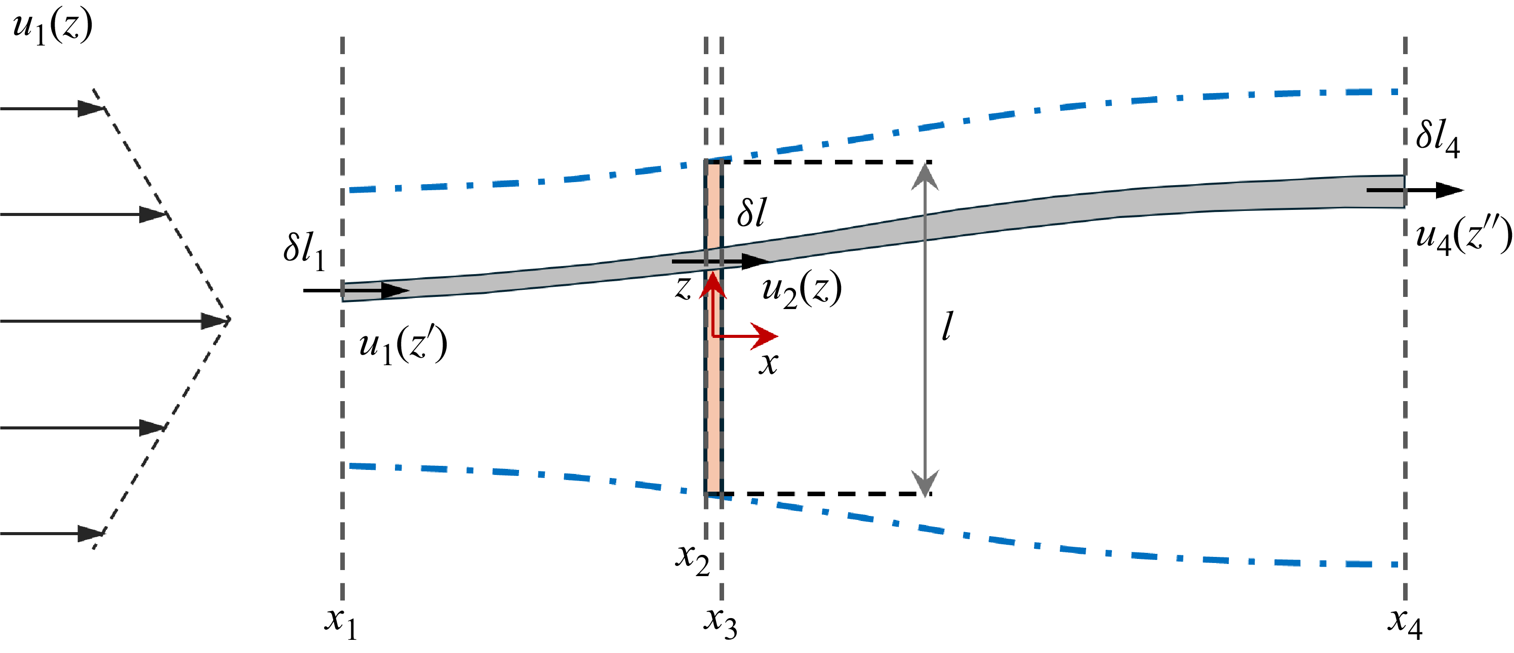
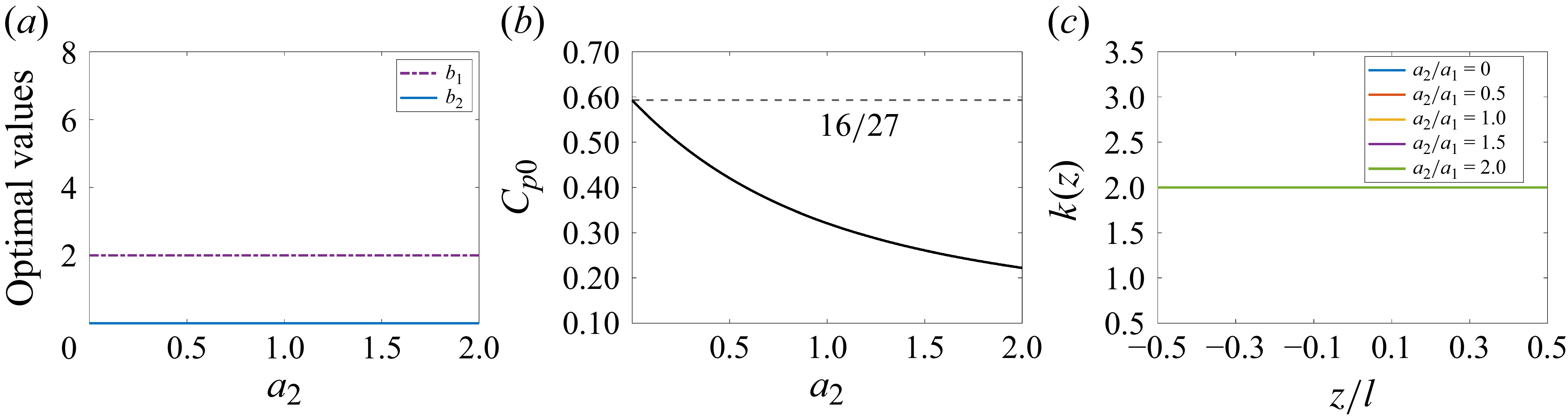
 a2⩾0
a2⩾0 Cp0
Cp0 a
a b1
b1 b2
b2 a2
a2 b
b a2
a2 c
c a2
a2
 a2⩾0
a2⩾0 Cp
Cp a
a b1
b1 b2
b2 a2
a2 b
b a2
a2 c
c a2
a2
 a2⩾0
a2⩾0 Cp
Cp a
a b1
b1 b2
b2 a2
a2 b
b a2
a2 c
c a2
a2
 a2⩽0
a2⩽0 Cp
Cp a
a b1
b1 b2
b2 a2
a2 a2=−1.34
 b
b a2
a2 c
c a2
a2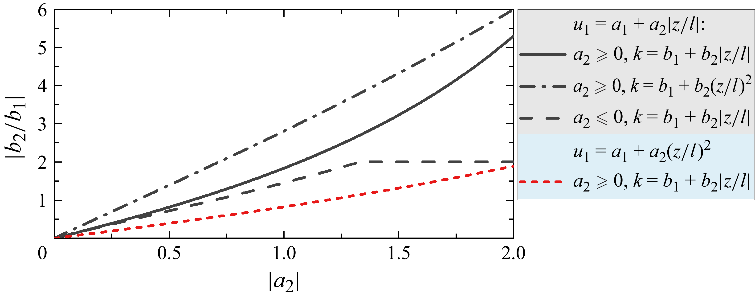
 b2/b1
b2/b1 |a2|
|a2| Cp
Cp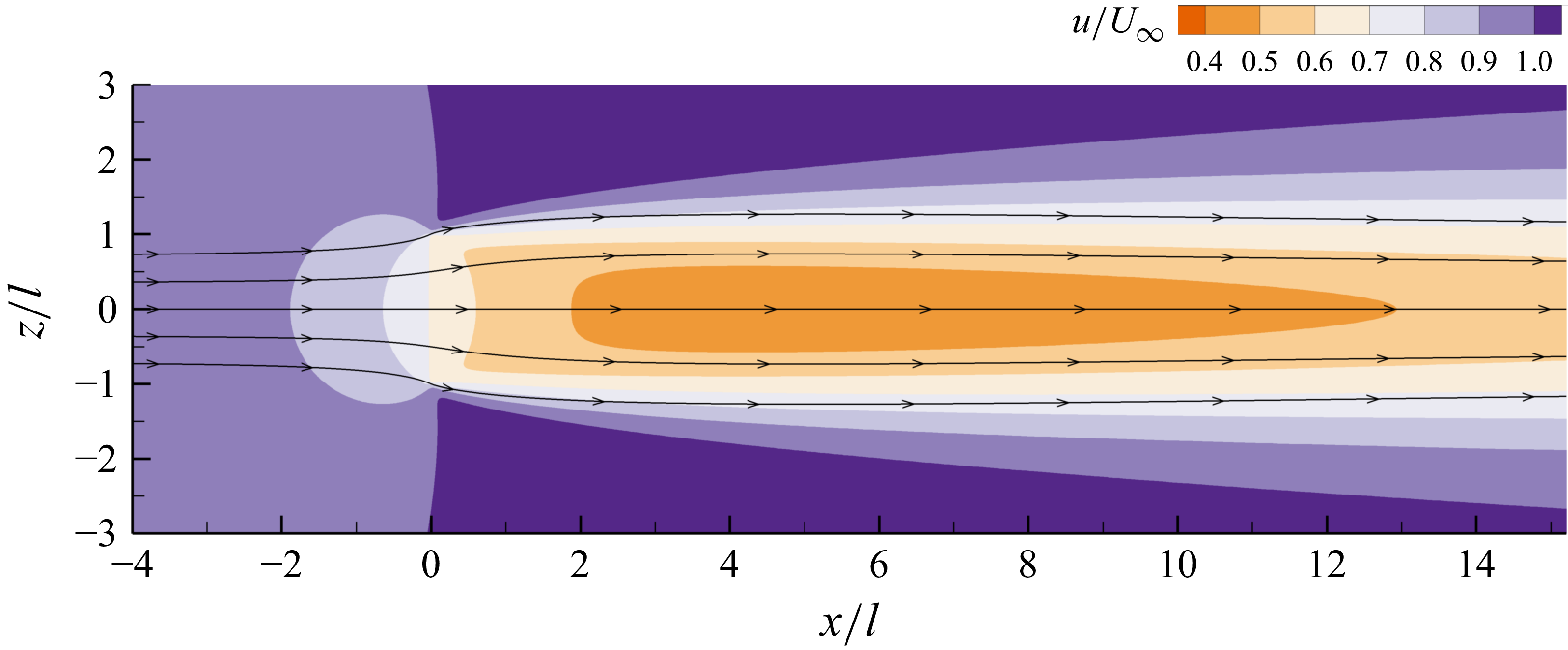
 k(z/l)=2
 Re=100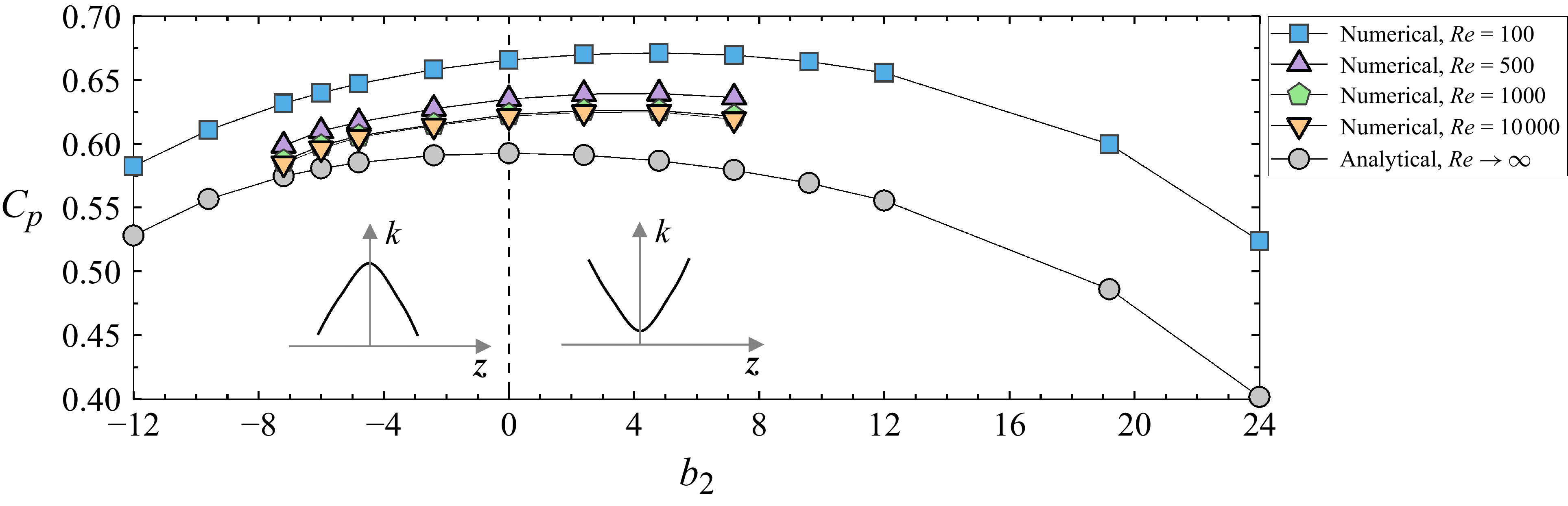
 k(z/l)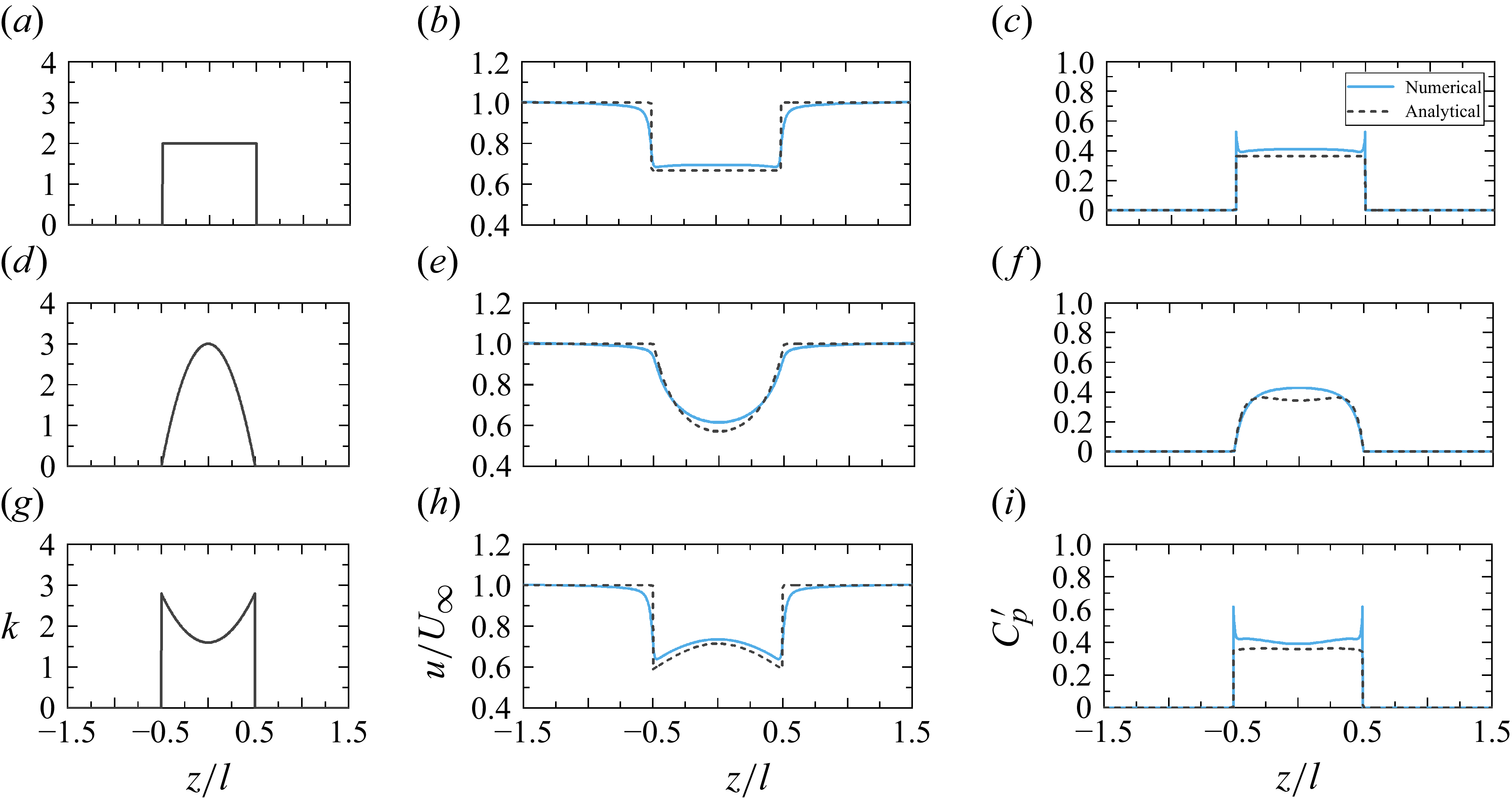
 (b,e,h)
 x/l=0
x/l=0 (c,f,i)
 x/l=0
x/l=0 z/l=[−0.5,0.5]
 Re=100
 b1=2,b2=0
 (a,b,c)
 b1=3,b2=−12
 (d,e,f)
 b1=1.6,b2=4.8
 (g,h,i)
 k
k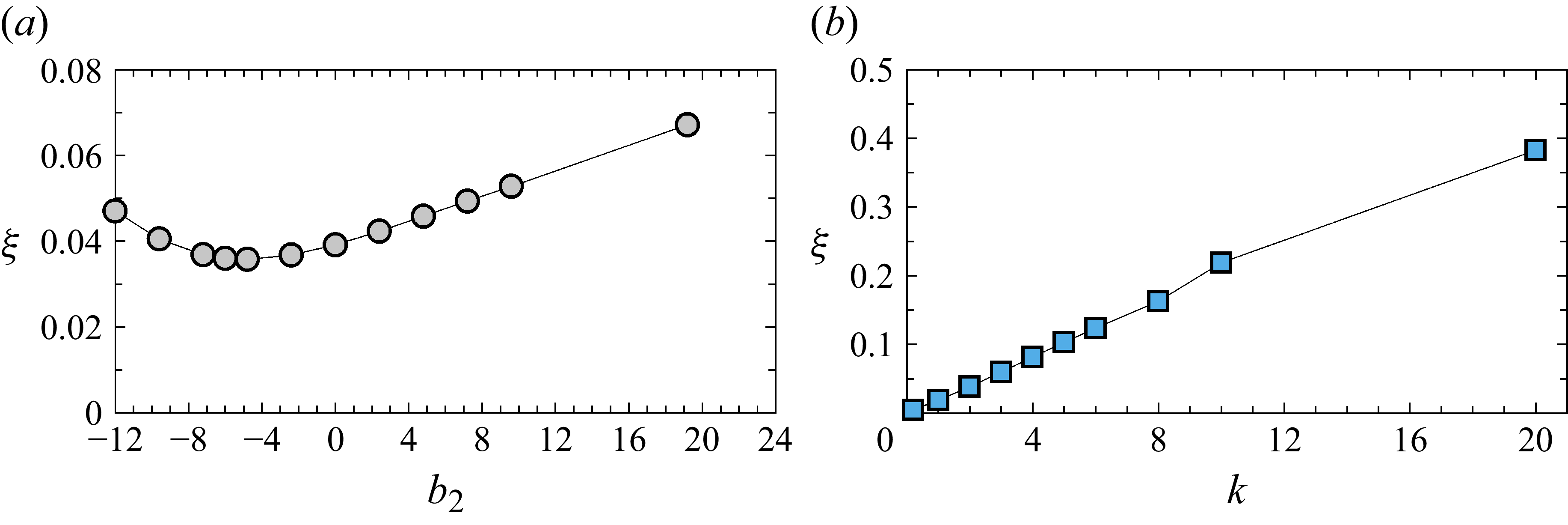
 (a)
(a) ξ
ξ b2
b2 k
k (b)
(b) ξ
ξ k
k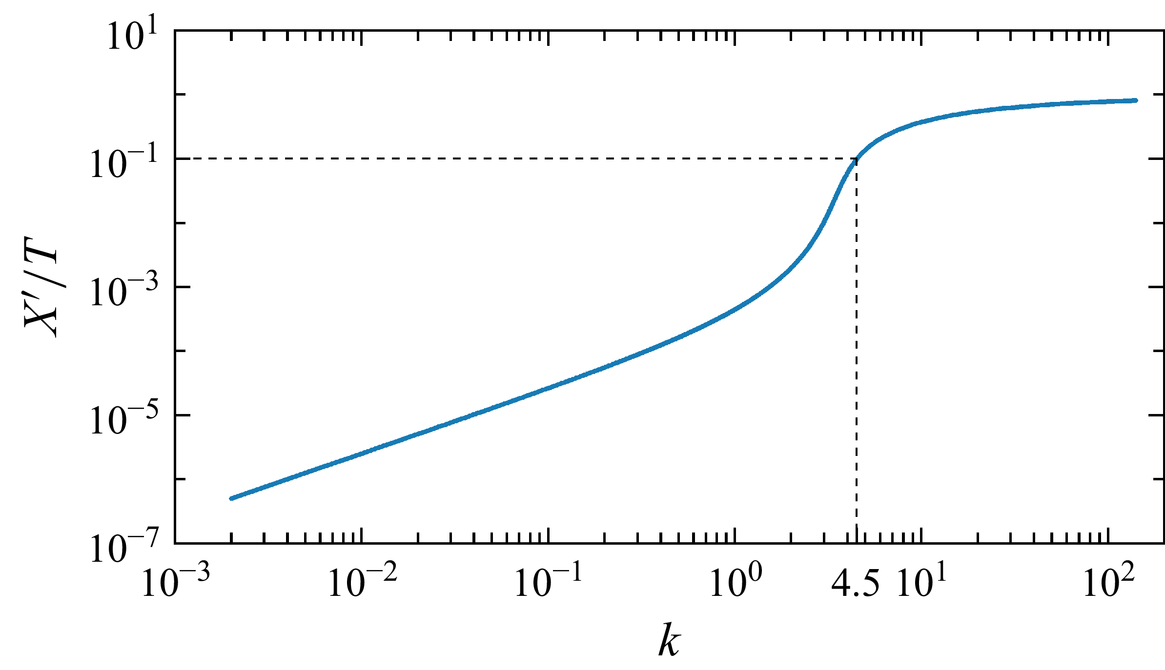
 X′/T
X′/T k
k X′/T
X′/T k
k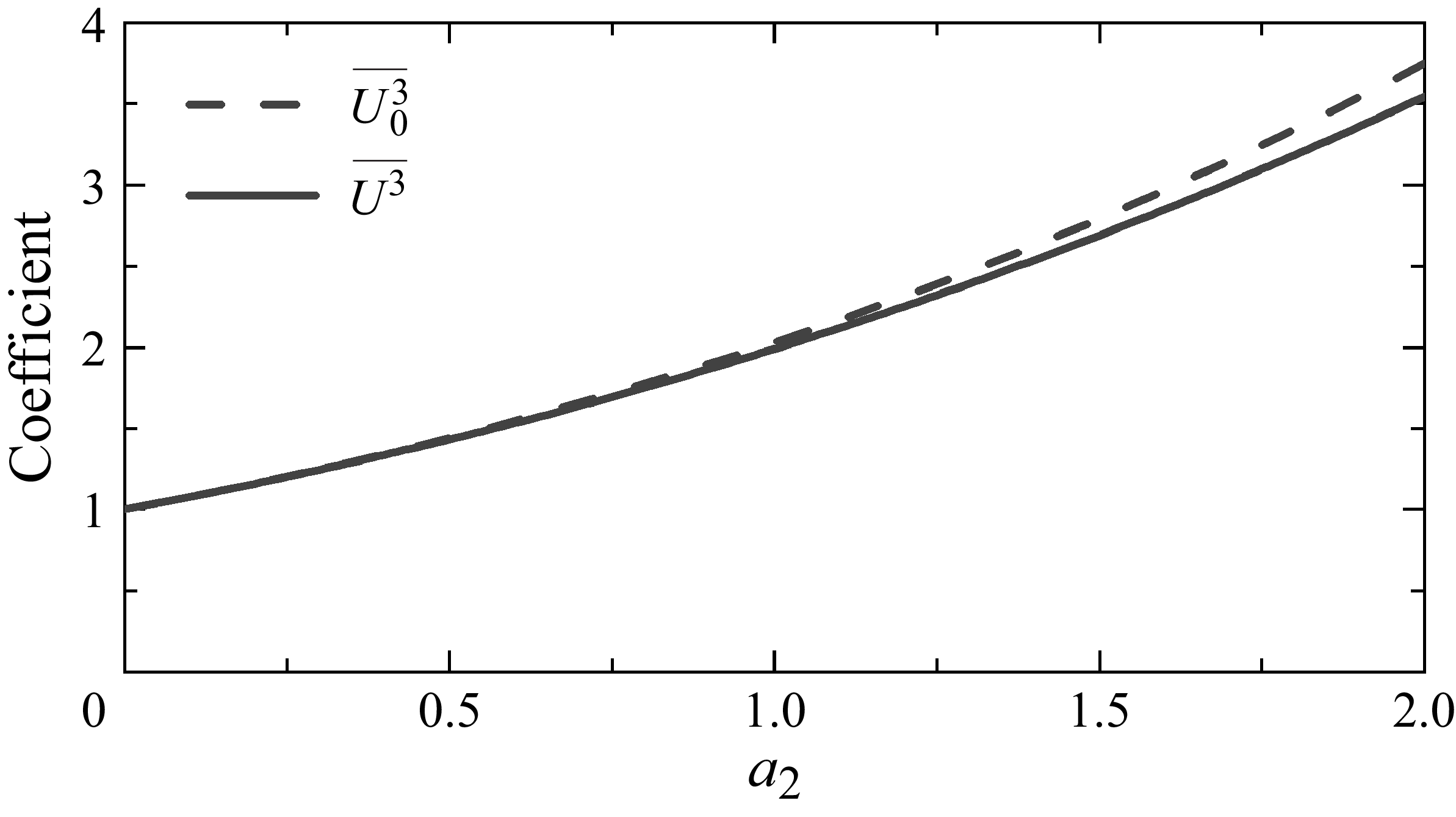
 U03¯
U03¯ U3¯
U3¯ a2
a2 Cp
Cp
 Open access

