


Impact Statement
-
• Use of system for automated quality control (SaQC) combined with machine learning algorithms on meteorological data
-
• Comparison of three types of autoencoders
-
• Evaluation of detected anomalies
1. Introduction
1.1. Overview
Ensuring the quality of meteorological observations is critical for accurate forecasting, climate analysis, and downstream applications. Traditional quality control (QC) systems rely on rule-based methods and expert intervention, but these approaches are increasingly challenged by the growing volume and complexity of observational data. In recent years, machine learning (ML) has emerged as a promising tool to enhance QC by identifying subtle patterns and anomalies that may escape conventional techniques.
Met Éireann has begun exploring ML-based QC methods to complement its existing systems. These efforts aim to automate anomaly detection, reduce manual workload, and improve the timeliness and reliability of data used in operational forecasting and research. While ML-based QC is still an emerging field, several meteorological services, including ECMWF, MeteoSwiss, and Met Norway, which will be discussed in more detail later, have developed innovative systems that offer valuable lessons and potential pathways for adaptation.
This paper presents Met Éireann’s recent work in developing ML-based QC systems, including the integration of open-source tools such as Titan (Båserud et al., Reference Båserud, Lussana, Nipen, Seierstad, Oram and Aspelien2020) and the application of deep learning models to observational data. It also outlines the operational requirements for QC, reviews the evolution of QC techniques across leading organizations, and highlights the novelty and differentiation of Met Éireann’s approach compared to existing systems.
The remainder of Section 1 is organized as follows:
-
• Section 1.2: QC concepts and operational requirements
-
• Section 1.3: Evolution of QC techniques by leading organizations
-
• Section 1.4: ML approaches and Met Éireann’s recent work
1.2. QC concepts and requirements
Automated QC systems must meet operational requirements while remaining adaptable to evolving data sources and user needs. To design such systems, it is important to understand both the standards set by international bodies and the practical constraints faced by national meteorological services.
The World Meteorological Organization (2021a) has specified certain standards for QC on meteorological observation data to ensure consistency in meteorological datasets worldwide. According to World Meteorological Organization (2021b) the five main categories of QC are:
-
• Constraint tests: Ensure values fall within instrument measurement capabilities.
-
• Consistency tests: Compare data across time and space for internal coherence.
-
• Heuristic tests: Apply expert knowledge to assess plausibility.
-
• Data provision tests: Detect missing or stuck sensor readings.
-
• Statistical tests: Identify long-term trends and climatological anomalies.
These tests may be applied manually, semi-automatically, or fully automatically, depending on the station type, elevation, and data volume. Crucially, flagged data should be retained alongside corrected values to preserve traceability.
Met Éireann currently collects data from two main automatic meteorological networks, with additional data collected from airports, weather balloons, and a new automatic aviation observation network (AWOS), among others.
1.2.1. The Unified Climate and Synoptic Observations Network (TUCSON)
This is Met Éireann’s operational network, comprising 20 stations, and forms part of the WMO Global Basic Observing Network (GBON). The data from it are used for forecasting and climatological research. TUCSON provides comprehensive measurements including temperature (air, grass, soil, and earth), humidity, pressure, wind, solar radiation, and rainfall. Each station includes dual sensors for redundancy. TUCSON data undergo rule-based QC for basic anomaly detection (Fitzpatrick et al., Reference Fitzpatrick, Broderick, Clancy, Creagh, Curley, Gill, Lally, Li, Nic Guidhir, O’Keefe, O’Leary and Conall2021), with manual QC applied to meet WMO’s heuristic and statistical requirements. However, manual QC is resource-intensive and increasingly unsustainable given the volume of data.
1.2.2. Climate automation and modernization project (CAMP)
This network currently consists of 78 stations classified into three categories: A) which measure only air and grass temperature, B) which measure air, grass, and soil temperature (at 5, 10, and 20 cm depth), and C) which measure air, grass, soil, and earth temperature (at 30, 50, and 100 cm depth). Each station has one sensor of each type, and the stations are too far apart from each other and the TUCSON stations to make valid comparisons to neighboring stations. The 1-minute data from the CAMP stations are currently not quality-controlled and therefore underutilized in Met Éireann’s operations.
For all types of observations, it is essential to provide a form of automated QC to ensure timely delivery of the highest quality data and maximize the coverage of measurements across Ireland. In developing such a system, it is useful to learn from other organizations that have already implemented QC systems.
Among the interesting use cases for quality control is one developed by MeteoSwiss (Sigg, Reference Sigg2020), which employs a plausibility rating system using a sequential Naïve Bayes algorithm, comparing automated test outcomes with expert decisions to assign confidence scores. This allows users to select data based on desired accuracy levels.
While optimally all data should be 100% accurately quality-controlled immediately upon receipt from the instruments, realistically certain datasets may take longer to process, as many are still manually entered, such as rainfall data. Also, for some users it may be beneficial to have raw or almost raw data, while other applications, such as climate research, require the highest level of quality control that has been confirmed by an expert. A system such as that used by Meteo Swiss could benefit Met Éireann as well by giving users a choice of data quality level appropriate for their needs.
Met Norway has developed a Python library for quality control called Titan (Båserud et al., Reference Båserud, Lussana, Nipen, Seierstad, Oram and Aspelien2020), which allows for grouping of nearby stations to compare measurement values. It is opensource and freely adaptable to any use case. For this method to be effective, there must be at least three, but preferably five stations that can be grouped together within a defined radius. Ireland does not currently have a sufficiently dense network of stations for this to work, however it should be considered for use on crowd-sourced data in the future, and indeed some work has already been done in this area (Nagle, Reference Nagle2021; Fennelly, Reference Fennelly2024; Walsh, Reference Walsh2025).
The Helmholtz Institute for Environmental Research (UFZ) has developed a System for Automated Quality Control (SaQC) designed to flag time series environmental data (Schmidt et al., Reference Schmidt, Schäfer, Geller, Lünenschloss, Palm, Rinke, Rebmann, Rode and Bumberger2023). This is an opensource Python library designed to be adaptable to any environmental observation network. It allows users to define parameters for flagging data and provides in-built statistical algorithms to detect outliers and correct data while allowing for customization. This system helps to make QC processes traceable and reproducible, with easily configurable flagging mechanisms.
Increasingly, meteorological organizations are turning toward crowd-sourced data to enhance their forecasts. A study conducted in the Pacific Northwest of the United States (Madaus et al., Reference Madaus, Hakim and Mass2014) aimed to use pressure data from outside sources, including altimeter data from aircraft, to improve not only the pressure forecasts but also to gain a better understanding of the atmosphere. Atmospheric pressure is a relatively stable and easy variable to QC, and therefore well suited to machine learning.
Another interesting study (Niu et al., Reference Niu, Yang, Zheng, Cai and Qin2021) focused on anomaly detection on crowd-sourced rainfall data, using supervised and unsupervised methods including k-nearest neighbor (kNN), multilayer perceptrons (MLPs), and isolation forest (iForest). This demonstrates a potential method of QC on rainfall data, which so far has been largely unexplored due to its random and intermittent nature.
Similarly the EUMETNET (European Meteorological Network) published a report for a test case on crowd sourced data QC (Norwood-Brown and Molyneux, Reference Norwood-Brown and Molyneux2019) for personal weather stations, including temperature, pressure, and wind. They found that temperature and pressure were relatively stable and predictable, however wind created problems, especially when sensors were not ideally placed. There is still much room for further development in this area, but it is useful to learn from others what works and what does not.
Perhaps one of the most advanced and effective machine learning techniques for quality control on meteorological data is currently being used by the European Centre for Medium-range Weather Forecasting (ECMWF) (Dahoui, Reference Dahoui2023). In this case a Long Short-Term Memory (LSTM) autoencoder is employed to quality control meteorological surface and satellite data. There are two separate algorithms, one for long-term, looking at the entire year of data to detect, for example, sensor drift, and one for short-term, looking at only a few days at a time for anomaly detection such as extreme temperature values. It is run on all observation types separately, and the combined results are fed into a random forest classifier which categorizes the flagged data by severity and possible cause. The labels created by the classifier are then used to inform future events of the same type. This is currently only applied through post-processing this data but is envisioned to be applied to live streaming observational data soon.
These examples underscore the importance of tailoring QC methods to specific variables and data sources. They also highlight the growing role of automation and modularity in QC design. As meteorological services increasingly incorporate crowd-sourced and high-frequency data, scalable and adaptable QC frameworks, potentially enhanced by machine learning, are becoming essential.
1.3. ML approaches and Met Éireann’s recent work
Met Éireann has conducted several exploratory studies to assess the feasibility of machine learning (ML) for automating quality control (QC) of meteorological data. While these studies are currently unpublished and exist as internal reports or academic theses, they provide a valuable foundation for future operational systems and highlight the potential of ML-based QC in the Irish context.
There have so far been two deep learning approaches for QC. Horan (Reference Horan2021) developed a long short-term memory (LSTM) autoencoder to detect anomalies in temperature data from the TUCSON station in Athenry. The year 2014 was selected due to its high incidence of manually flagged anomalies. While the model showed promise, it was sensitive to threshold settings and prone to false positives. The study was constrained by limited computational resources but demonstrated the viability of LSTM-based QC for time series data.
O’Donoghue (Reference O’Donoghue2023) extended this work by testing both autoencoders and variational autoencoders (VAEs) on TUCSON temperature data. Two approaches were evaluated: one using only date–time and temperature, and another using paired air and grass temperature readings. Both methods successfully detected manually inserted anomalies, with the VAE showing greater robustness due to its probabilistic latent space representation. Notably, the model identified anomalies in grass temperature even when trained to detect air temperature anomalies, suggesting strong generalization capabilities.
In addition to the machine learning aspect of QC, initial work by Nagle (Reference Nagle2021) explored the use of Titan, an open-source Python library developed by Met Norway, to apply QC to crowd-sourced data from the UK Met Office’s Weather Observations Website (WOW). Titan uses a “buddy check” algorithm that compares measurements from nearby stations to identify anomalies. Although promising, the study found that the density of WOW stations in Ireland was insufficient for effective spatial grouping. With WOW scheduled to be discontinued by 2026, future efforts may focus on alternative networks such as Netatmo (2025), which offer higher station density in urban areas.
Building on this, Fennelly (Reference Fennelly2024) applied Titan to the 2020 Netatmo data for Ireland. The results were encouraging in cities like Dublin and Cork, but sparse coverage in rural regions, particularly in the northwest, limited the method’s effectiveness.
These studies suggest that Titan may be best suited for QC of crowd-sourced data in densely populated areas and could be integrated into a hybrid system combining spatial and temporal anomaly detection. Titan can also be used in conjunction with machine learning, providing a rule-based baseline QC before feeding data into an ML algorithm, or using the flags generated via Titan for feature engineering in ML models to improve prediction accuracy.
1.4. Anomaly detection and future directions
Anomaly detection is a central component of automated quality control (QC) systems, particularly when dealing with high-frequency or crowd-sourced meteorological data. Traditional rule-based methods often struggle to detect subtle or context-dependent anomalies, especially in complex datasets. Machine learning (ML) offers a powerful alternative by learning patterns directly from the data and identifying deviations that may indicate sensor errors, transmission faults, or environmental outliers.
Among unsupervised ML methods, autoencoders, particularly long short-term memory (LSTM) and variational autoencoders (VAEs), have shown strong potential for anomaly detection in meteorological time. These models compress input data into a latent representation and attempt to reconstruct it. The difference between the input and output (reconstruction error) can be used to flag anomalies. VAEs, in particular, offer robustness by mapping inputs to a probability distribution, making them more tolerant of natural variability in unseen data.
Met Éireann’s internal studies have demonstrated the feasibility of using these techniques for QC. These studies, while limited by computational resources, provide a strong proof of concept for operational deployment.
ECMWF has implemented a complex system that combines long-term and short-term LSTM autoencoders with a random forest classifier to categorize anomalies by severity and cause for the vast number of data streams it receives. By contrast, Met Éireann’s needs are more targeted and resource-constrained, so a modular and adaptable approach that could be scaled incrementally would be ideal.
Looking ahead, Met Éireann aims to develop a real-time ML-based QC system that:
-
• Integrates both national and crowd-sourced data sources
-
• Supports multiple QC levels tailored to user needs
-
• Combines spatial and temporal anomaly detection
-
• Is transparent, reproducible, and easy to maintain
Such a system would not only improve the quality and timeliness of observational data but also reduce the burden of manual QC, enabling expert staff to focus on higher-level analysis and system development. With further investment in infrastructure and collaboration with international partners, Met Éireann is well-positioned to lead in the operational application of ML for meteorological QC.
2. Method
2.1. Design
We propose a multi-phase quality control (QC) framework for meteorological observations that integrates automated rule-based checks, machine learning (ML)-based anomaly detection, and expert human validation. The system is designed to identify and address common data issues such as missing values, sensor malfunctions (e.g., stuck sensors), and extreme outliers, while also capturing more subtle anomalies through data-driven methods.
The QC workflow is implemented on the SaQC platform and proceeds through the following stages:
Data Ingestion and Preprocessing: Observational data are ingested and pre-processed using Python scripts to ensure format consistency and readiness for QC procedures.
Automated Rule-Based Checks: Initial QC is performed using SaQC’s built-in functions and customized configuration files. These checks include plausibility tests, range validations, and temporal consistency assessments. Data failing these checks are flagged and excluded from subsequent ML analysis.
Machine Learning-Based Anomaly Detection: The filtered dataset is subjected to anomaly detection using the most suitable ML algorithm identified through prior benchmarking. Anomalies are flagged using a custom function integrated within SaQC.
Expert Review and Correction: Flagged observations are reviewed by human QC experts who assess the validity of the ML-generated flags and determine appropriate corrective actions. These may include interpolation, drift correction, pattern recognition, or predictive modelling. Corrections can be applied either automatically via SaQC or manually by experts.
Data Versioning and Flagging: Multiple levels of data quality are made available to end users, ranging from raw observations to flagged and corrected datasets. All original values are retained, and flags are assigned to indicate the nature and source of any corrections applied.
Currently, a prototype of this system has been deployed at Met Éireann to perform basic automated checks on observational data. Although not yet operational, it is being used to prepare datasets for ML-based anomaly detection. Initial efforts have focused on air temperature data from the TUCSON network, selected for its simplicity and suitability for comparative analysis.
Figure 1 illustrates the overall workflow of the proposed QC system.
Workflow diagram for proposed automated QC system.

2.2. Concept
This study compares the performance of three machine learning algorithms in detecting temperature anomalies. It uses the same TUCSON data from the Athenry station in the previous studies conducted at Met Éireann. The key difference is that previous studies trained their algorithms on quality-controlled data but tested them on raw data or trained and tested on only the raw data (with some filtering of stuck, missing, or extreme values). In contrast, we tested our algorithms on fully quality-controlled data—assuming it to be flawless—and applied the best configuration to the raw data.
We compared the performance of the autoencoder, variational autoencoder, and LSTM autoencoder from the previous studies.
2.3. Model selection and rationale
In this study, we evaluated the performance of three deep learning architectures previously explored in internal research at Met Éireann: the standard autoencoder (AE), the variational autoencoder (VAE), and the long short-term memory autoencoder (LSTM). These models were selected based on preliminary results indicating promising anomaly detection capabilities and their relatively straightforward implementation. Although generative adversarial networks (GANs) were initially considered (Bashar and Nayak, Reference Bashar and Nayak2023), they were excluded due to their high computational demands and limited interpretability, which pose challenges for operational deployment and scientific transparency. What follows is a brief description of each model, including the advantages, assumptions, and limitations of implementing them.
2.3.1. The standard autoencoder
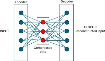
According to Rezapour (Reference Rezapour2019), an autoencoder is a neural network that is trained to minimize the loss between an original input and its reconstruction using unsupervised learning. It consists of an encoder that compresses input data into a lower-dimensional latent space and a decoder that reconstructs the original input from this representation, as depicted in Figure 2. Anomalies are identified by comparing the reconstruction error between input and output.
Architecture of a standard autoencoder.

Advantages of using this type of machine learning model are its relative simplicity and low computational cost compared to more complex models. However, it assumes that training data exhibit normal behavior and has limited ability to model temporal dependencies in time series data.
2.3.2. The variational autoencoder
An and Cho (Reference An and Cho2015) describe the VAE as an example of a directed probabilistic graphical model which maps inputs to a probability distribution of the latent variables, thus making it more robust to slight but valid variations in unseen input data. In the standard autoencoder, the latent variables are calculated in a deterministic fashion, with the mappings of the input to its representation in the latent space is point to point. This can make autoencoders brittle to valid inputs that are marginally different from the training data.
A variational autoencoder assumes that latent variables follow a known prior distribution (usually Gaussian) and is limited by more complex training and tuning than a standard autoencoder.
2.3.3. The LSTM-autoencoder
LSTM autoencoders incorporate recurrent neural networks (RNNs), specifically LSTM units, to model sequential dependencies in time series data. The encoder processes the input sequence to produce a compressed representation, and the decoder reconstructs the sequence from this representation (Homayouni et al., Reference Homayouni, Ghosh, Ray, Gondalia, Duggan and Kahn2020).
They are particularly suited to finding patterns in timeseries data, assuming temporal patterns in normal data are consistent and learnable. The main limitations of LSTM models include their sensitivity to hyperparameter settings and sequence length, as well as their relatively high computational cost and longer training times compared to standard and variational autoencoders, particularly when dealing with long sequences.
2.4. Data preparation and model configuration
Quality-controlled 1-minute data for the years 2010–2022 excluding 2014 from the TUCSON Athenry station, were used for training the algorithms, and 2014 was used for testing. The data were pre-processed to maintain the cyclical nature of the month, day, and hour fields, as cos and sin representative of these fields. As an example, the formula used for the ‘month cosine’ field was:
 $$ \mathrm{mont}{\mathrm{h}}_{\mathrm{cos}}=\cos \Big(\left(2\unicode{x03C0} \ast \frac{\mathrm{month}}{\max \left(\mathrm{month}\right)}\right) $$
using the method described by O’Donoghue (Reference O’Donoghue2023). The data were de-seasonalized and de-trended and a standard scalar applied using the sklearn (Pedregosa et al., Reference Pedregosa, Varoquaux, Gramfort, Michel, Thirion, Grisel, Blondel, Prettenhofer, Weiss and Dubourg2011) and statsmodels (Seabold and Perktold, Reference Seabold and Perktold2010) modules in Python. The training data were split 80/20 into training/validation. The algorithm hyperparameters were tuned using hyperopt (Bergstra et al., Reference Bergstra, Komer, Eliasmith, Yamins and Cox2015) in MLflow (2025) to determine the best batch size and number of epochs, and latent dimensions for the autoencoders.
The results of the hyperopt tuning showed that the best parameters to use for all three algorithms were a batch size of 500, 150 epochs, and 2 latent dimensions. The algorithms were trained on a laptop with 16GB RAM and 4 CPU cores.
The machine learning algorithms were developed in Python and used Tensorflow (Abadi et al., Reference Abadi, Agarwal, Barham, Brevdo, Chen, Citro, Corrado, Davis, Dean, Devin, Ghemawat, Goodfellow, Harp, Irving, Isard, Jozefowicz, Jia, Kaiser, Kudlur, Levenberg, Mane, Schuster, Monga, Moore, Murray, Olah, Shlens, Steiner, Sutskever, Talwar, Tucker, Vanhoucke, Vasudevan, Viegas, Vinyals, Warden, Wattenberg, Wicke, Yu and Zheng2015) and Keras (Reference Chollet2025) modules for machine learning, Pandas for data wrangling, and the SaQC library for the quality control platform.
3. Results
3.1. Testing quality-controlled data
When evaluating the effectiveness of an algorithm for anomaly detection, a typical approach is to check how many true positives (anomalous data), true negatives (non-anomalous data), false positives (non-anomalous data incorrectly flagged as anomalous), and false negatives (anomalous data incorrectly flagged as non-anomalous) the algorithm finds. This assumes that there are known anomalies in the dataset. However, in this study, the algorithms have been trained and tested on quality-controlled data, which is assumed to be error-free and accepted as ground truth for the purposes of these experiments. Any data flagged as an anomaly by the algorithm would thus by default be considered a false positive.
After training on all other available years, the three algorithms were tested on the quality-controlled, one-minute air temperature data for the year 2014 at Athenry. This was done by using SaQC to first filter out any extreme, missing, or stuck sensors, which, in the case of quality-controlled data, was none, but nevertheless standard practice, and then applying the trained models to the data. Each algorithm produces an output of predicted values, which can then be used to calculate the reconstruction error, in this case, mean squared error (mse), using the formula:
 $$ \mathrm{mse}={\left(\mathrm{original}\ \mathrm{value}-\mathrm{predicted}\ \mathrm{value}\right)}^2 $$
To identify anomalous observations, a threshold was applied to the reconstruction error, calculated as the mean squared error between the input and output of each model. For each model, the threshold was set at the 99th percentile of the mse distribution derived from the validation dataset. This approach assumes that the majority of the data represent normal conditions, and that the upper tail of the error distribution corresponds to statistically significant deviations.
Several threshold levels (ranging from the 95th to 99th percentile) were evaluated during preliminary testing. The 99th percentile was selected as the optimal threshold for this study, as it provided the best balance between minimizing false positives and capturing meaningful anomalies in air temperature data. While this approach inherently flags approximately 1% of the data as anomalous, it was found to be the most effective in identifying subtle but valid deviations without overwhelming the expert review process.
As the plots in Figure 3 show all three algorithms are flagging similar numbers of datapoints as anomalies, however on closer inspection, the points being flagged are not the same. The variational autoencoder (VAE) and long-short-term-memory (LSTM) autoencoder are most similar in the points they flag. The VAE flags 263 points and the LSTM flags 266 points, with only 10 points being different. The autoencoder (AE) flags are substantially different from the other two algorithms, although, like the VAE, it flags 263 points; these differ in 45 observations from the ones flagged by the other algorithms in January, May, and October.
Air temperature time series of Athenry QC data (dark blue line) with red dots marking points where mean squared error exceeded the 99th percentile threshold for autoencoder (AE), variational autoencoder (VAE), and long-short-term-memory (LSTM) autoencoder on left axis and mean squared error (MSE) (light blue) with 99th percentile threshold (light red) on right axis.

Machine learning algorithms often flag false positives when a dataset is imbalanced, meaning anomalies are extremely rare, as should be the case when using quality-controlled data for testing. It is up to the user to define how many false positives are acceptable, depending on how the data will be used. With the air temperature data, the number of flagged datapoints constitutes only 0.05% of the data in one year, which would not substantially affect the workload of a quality control expert.
3.2. Experimenting with the LSTM timesteps
In the previous example, the LSTM had been set to 60 timesteps for its long-term memory, which in this case equates to 60 minutes, the frequency of data passed to the algorithm concurrently. As it is unlikely that any patterns will be detected in only one hour of air temperature data, the long-term memory capability of the LSTM required further investigation.
Using computing resources of 8 CPU cores and 32 GiB of memory on the European Weather Cloud (EWC) (European Weather Cloud, 2024) and the Keras Tuner Python package (Invernizzi et al., Reference Invernizzi, Long, Chollet, O’Malley and Jin2019), further testing was done on the LSTM algorithm.
In the case of the LSTM autoencoder, the MSE was computed over sequences of varying lengths to assess the impact of temporal context on anomaly detection. Figure 4 illustrates the flagged anomalies in the 2014 quality-controlled Athenry air temperature dataset using LSTM models trained with sequence lengths of 60 minutes (1 hour), 1440 minutes (1 day), 2880 minutes (2 days), and 4320 minutes (3 days). Due to computational constraints, three days with a batch size of five was the maximum feasible sequence length, as LSTM’s store activations for each timestep during back propagation, which leads to higher memory usage with longer sequences. Table 1 shows the performance metrics of the algorithms for training and testing. The AE, VAE, and LSTM 1-hour models were initially trained on a laptop using the parameters described in Section 2.4. The LSTM 1-hour model was then retrained on the EWC, first with the same parameters as the laptop, and again using the parameters applied to the longer LSTM sequences. Testing for all models was conducted on the laptop.
Quality-controlled Athenry air temperature time series for 2014 (blue line) with red dots indicating points where the mean squared error exceeded the 99th percentile between the original and reconstructed data using the LSTM with different timesteps (in number of minutes).

Performance metrics for training and testing of the models

As the sequence length increased, the number of flagged anomalies decreased: from 266 (1-hour sequences) to 51 (1-day), 38 (2-day), and 36 (3-day). Notably, the most substantial reduction occurred between the 1-hour and 1-day configurations, while the difference between the 2-day and 3-day models was marginal. This suggests that incorporating longer temporal context improves the model’s ability to distinguish between normal variability and true anomalies, up to a point of diminishing returns.
3.3. Application to non-QC data
As mentioned previously, all TUCSON stations are equipped with two sensors for each measurement type, to provide backup and overlap in case a sensor fails or diverges significantly. The quality-controlled dataset will show only one value, which is normally sensor 1 unless a problem occurred with that sensor. In July of 2014, air temperature sensor 1 failed at Athenry station, producing a series of extreme or impossible temperature values resulting in either manual corrections or switching to sensor 2.
This section will apply the LSTM autoencoder trained with 4320 (3 days) timesteps on quality-controlled data to the raw one-minute 2014 Athenry air temperature data from sensor 1, and assess the accuracy of the model based on what are considered
-
• True Negatives (data that are not manually flagged).
-
• True Positives (data that are manually flagged, corrected, or use sensor 2 in the quality-controlled set).
-
• False Positives (data which are flagged by the algorithm but not manually flagged).
-
• False Negatives (data which are not flagged by the algorithm but have manual flags or corrections in the quality-controlled dataset).
Figure 5 shows the raw one-minute air temperature time series for Athenry in 2014, with 678 datapoints flagged where the MSE exceeded the 99th percentile threshold. It is noteworthy that 20 of these flags correspond to the same LSTM-flagged datapoints in the quality-controlled data, and indeed to the events discussed in Section 4. There are 16 datapoints which are not flagged by the LSTM in the raw data that are flagged in by the LSTM in the QCd data. Of these, 10 datapoints used sensor 2 in the QC dataset, which could account for the LSTM’s higher reconstruction error in those cases. It is unclear why the remaining 6 datapoints were not flagged in the raw dataset.
Raw one-minute air temperature data for Athenry 2014 with red dots where MSE was above the 99th percentile threshold after fitting the LSTM autoencoder with 4320 timesteps (trained on quality-controlled data).

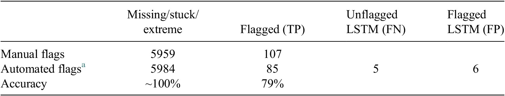
Table 2 presents a comparison between manual quality control (QC) flags and automated flags generated by the SaQC system, which combines basic sensor checks (for missing, stuck, and extreme values) with an LSTM-based anomaly detection algorithm. The results demonstrate high accuracy in identifying true anomalies in raw air temperature data from Athenry (2014).
Comparison between manual and automated flagging on raw air temperature data from Athenry in 2014

a Combined SaQC basic checks and LSTM MSE anomalies.
SaQC flagged more stuck sensor values than manual QC due to its systematic approach: human reviewers often only flag the first and last minute of a sequence of erroneous readings.
Of the 678 flagged observations in Figure 5, 593 were flagged as anomalous by the LSTM despite being marked as valid (flag = 0) in the manual QC. Of these:
-
• 555 used sensor 2 for QC, indicating a sensor switch not reflected in manual flags
-
• 12 were marked as “estimated” in the QC dataset
-
• 20 corresponded to meteorological events, discussed further in Section 4
-
• 6 occurred during gaps in the non-QC dataset (e.g., 26/01 at 06:13, 07:06, 07:07; 26/06 at 14:40–14:42), where LSTM struggled to predict values due to missing consecutive inputs (False Positives)
The LSTM correctly flagged 85 datapoints in the raw data, finding True Positives consistent with the manually flagged QC data 79% of the time.
Among the 107 manually flagged datapoints, 21 were “estimated” values. The LSTM did not flag 16 of these, as they were within acceptable deviation thresholds. The remaining 5 should be considered false negatives. For instance, on 16/07 at 23:06, the raw input was 22.15°C, the LSTM prediction was 22.34°C, while sensor 2 recorded 12.88°C, suggesting the input was anomalous. Interestingly, in each of these cases, the LSTM flagged the surrounding datapoints, likely due to its windowing mechanism. This behaviour suggests that isolated false negatives within a flagged sequence may still be identified during expert review.
4. Discussion
4.1. Meteorological anomalies
The LSTM’s long-term memory allows it to find patterns over time, and so its performance compared to the other algorithms is superior in flagging true positives consistent with human experts 79% of the time. Nevertheless, it still flags datapoints in the quality-controlled data. Looking more closely at these, it turns out that they were not flagged manually in the QC dataset, however when plotting the hours surrounding the flagged points, it is visible that there is a precipitous change in temperature in every case. The plots in Figure 6 illustrate this for three of the 16 days with flagged anomalies on which there are rapid drops in temperature, which the LSTM was unable to predict. Further investigation, which looked at related measurements such as solar radiation, relative humidity, wind speed, and rain at and around the flagged datapoints showed that these sudden changes are not anomalies related to faulty sensors, but rather possible cloud cover, fog, or rain that occurred at those times. These checks were conducted manually for each of the 36 flagged events in the LSTM three-day (4320 minute) test set (see Table 2). It is likely that the LSTM will detect these interdependencies between measurements if they are added as features to the algorithm in the future, making it better able to reconstruct the data.
Examples of the rapid temperature drops (highlighted in grey), which the LSTM flagged as anomalous in the quality-controlled data.

Each of the 36 flagged datapoints in the three-day LSTM set corresponds directly to some weather-related event. Looking at the other test sets, the two extra flagged points in the two-day set fall into the range of the event on 20/05 from Table 3 (the rest being the same as in the three-day set), but the 15 additional flagged points in the one-day set appear isolated and not related to any meteorological phenomena. Thus, it can be assumed that both the one-day and 60-minute sets contain a number of false positives, and the LSTM timesteps should be set to no less than 2880 minutes to minimise these. However, considering that the purpose of quality control is to find problems in the data, the 36 flagged datapoints in the three-day test set should be considered false positives as well, even though they are anomalous.
LSTM flagged anomalies with contributing factors and potential causes
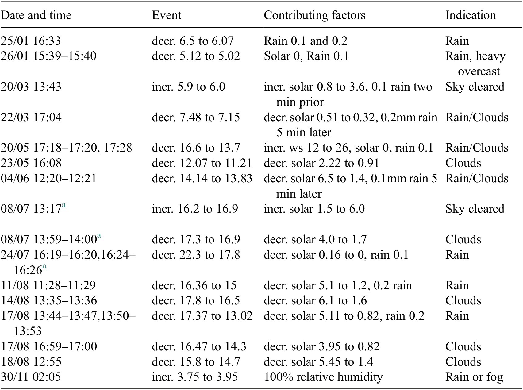
a Used Sensor 2 data.
4.2. Sensitivity to sensor differences
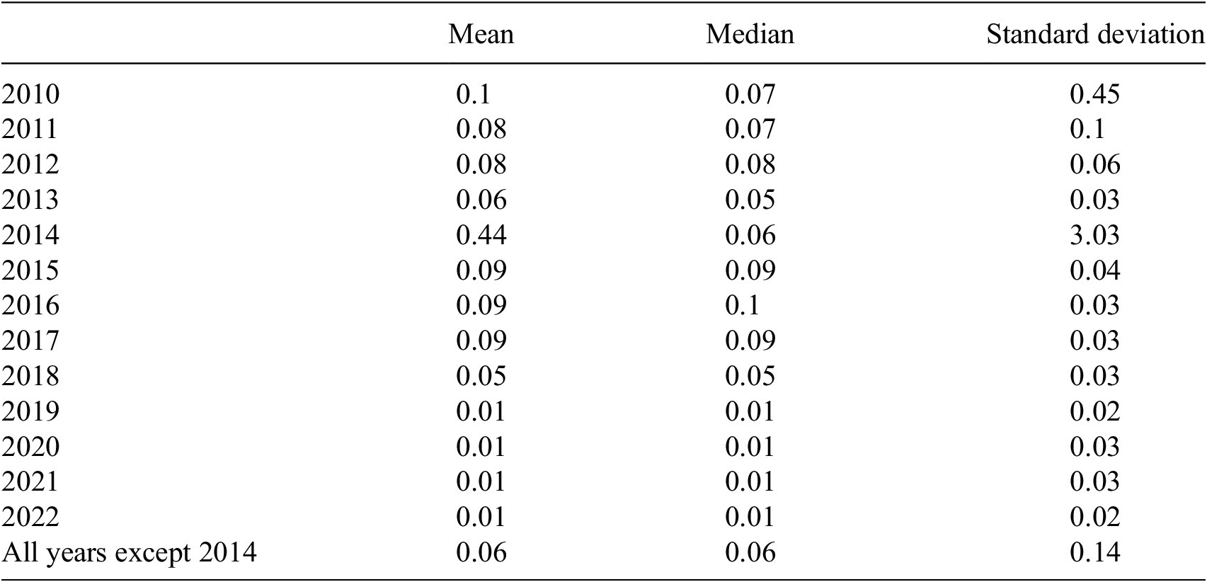
Another factor that seems to influence which datapoints the LSTM struggles to reconstruct is the difference between sensors in the cases where sensor 2 was used for the QC data, and thus the training data. Table 4 shows the mean, median, and standard deviation of the differences between the two air temperature sensors at Athenry for each year, as well as all years combined except 2014 (the years used for training the algorithm). Here, it is visible that 2014 is a clear outlier due to the failure of sensor 1, as all other years have means near 0 and low standard deviations. In some cases, the air temperature data for 2014 had to be estimated as neither sensor was providing plausible readings.
Mean, median, and standard deviation of the differences between air temperature sensor 1 and sensor 2 for each year at Athenry, including the combination of years used for training the LSTM (all years except 2014)

This will continue to be an issue with stations that have two sensors, however it will only surface when there is a significant deviation between the sensors, indicating a problem with one of them, which is what QC is meant to detect. Stations with only one sensor for each measurement will have to rely on other co-located measurements more to detect problems.
5. Conclusions and future work
While all of the algorithms performed similarly well in detecting anomalies, the LSTM stands out with its ability to find patterns in longer time periods, making it less likely to flag false positives in the data. The training time and memory requirements for longer LSTM sequences are higher than for the AE and VAE; however, training will likely only need to be conducted once per year. The training time for one station on 8 CPUs is under 4 hours and will be much less if implemented on a GPU.
Applying the LSTM algorithm, which had been trained on quality-controlled data, to the raw dataset yielded excellent results, with an ability to match good data (not flagged) with 99.6% accuracy, duplicate 79% of manual flags, producing only 5 false negatives and 6 false positives in the entire year.
While the data being flagged may not be caused by instrument failure or other quality-related issues, they do appear to be anomalous compared to the surrounding datapoints. The reason is almost always some related meteorological event, such as rainfall or cloud cover, that could cause a sudden change in temperature, as shown in each of the 36 flagged datapoints using the 3-day timestep LSTM algorithm. The algorithm’s sensitivity to such minor changes is impressive, as it can detect these changes in temperature as anomalous without any other inputs for comparison.
With the anticipated increase in computational resources at Met Éireann, it will become feasible to extend the evaluation of the LSTM-based anomaly detection algorithm to incorporate additional observational variables such as grass, soil, and earth temperatures, atmospheric pressure, and relative humidity, alongside air temperature. Integrating these variables may enhance the model’s ability to distinguish between normal and anomalous conditions by providing a more comprehensive environmental context.
Access to high-performance computing infrastructure would also enable an investigation into the impact of longer temporal windows on model performance. Preliminary comparisons suggest that a three-day timestep is sufficient for identifying isolated anomalous datapoints; however, further testing across varying window lengths could refine this assessment.
A more critical next step involves evaluating the generalizability of the trained model across different meteorological stations. This would help determine whether a universal model trained on aggregated data can effectively detect anomalies across diverse locations, or whether station-specific models, trained exclusively on local data, yield superior performance. Such insights are essential for developing scalable and robust quality control systems for environmental monitoring networks.
In conclusion, the use of an LSTM autoencoder with a three-day long-term memory in combination with the basic checks performed using SaQC appears to be a viable option for an automated quality control system at Met Éireann.
Open peer review
To view the open peer review materials for this article, please visit http://doi.org/10.1017/eds.2026.10030.
Acknowledgements
Special thanks to David Schäfer and Peter Lünenschloss at the Helmholz Centre for Environmental Research (UFZ) for help with the SaQC library and code.
Author contribution
Teresa K. Spohn: Conceptualization, Methodology, Software, Validation, Formal Analysis, Investigation, Writing-Original Draft. Eoin Walsh: Software, Investigation, Review and Editing. Kevin Horan: Software, Validation, Review and Editing. John O’Donoghue: Software, Validation, Review and Editing. Tim Charnecki: Resources, Data Curation, Review and Editing. Merlin Haslam: Resources, Project Administration, Review and Editing. Sarah Gallagher: Supervision, Funding Acquisition, Review and Editing.
Competing interests
The authors have no competing interests to this work
Data availability statement
The quality-controlled data used in this study are publicly available to download directly from Met Éireann on www.met.ie and the raw data are freely available upon request by emailing Database.Unit@Met.ie
Funding statement
This work was funded by Met Éireann


 Open access
Comments
Dear Editor,
Please consider this application paper, “A Machine Learning Approach to Quality Control on Meteorological Data” for publication in your journal, Environmental Data Science. The automation of quality control procedures using machine learning is of great interest to the field of Meteorology and Environmental Science generally, as it not only provides high quality data faster than previously possible, but detects anomalies that human experts are unable to see. My co-authors and I hope that this paper will help further the development of these systems.
Best Regards,
Teresa K. Spohn