


1. Introduction
While the study of two-dimensional irrotational inviscid water waves is classical with a long history (Haziot et al. Reference Haziot, Hur, Strauss, Toland, Wahlén, Walsh and Wheeler2022), there is growing interest in the theory of water waves with vorticity where finite-amplitude waves of interesting forms can exist even in the absence of either gravity or surface tension (Benjamin Reference Benjamin1962; Simmen & Saffman Reference Simmen and Saffman1985; Pullin & Grimshaw Reference Pullin and Grimshaw1988; Teles da Silva & Peregrine Reference Teles da Silva and Peregrine1988; Vanden-Broeck Reference Vanden-Broeck1994, Reference Vanden-Broeck1996; Sha & Vanden-Broeck Reference Sha and Vanden-Broeck1995; Constantin & Strauss Reference Constantin and Strauss2004; Groves & Wahlén Reference Groves and Wahlén2007, Reference Groves and Wahlén2008; Ehrnström Reference Ehrnström2008; Wahlén Reference Wahlén2009; Hur & Dyachenko Reference Hur and Dyachenko2019a , Reference Hur and Dyachenkob ; Hur & Vanden-Broeck Reference Hur and Vanden-Broeck2020; Hur & Wheeler Reference Hur and Wheeler2020). Since the presence of vorticity itself can influence the shape of a steadily translating wave structure, it is natural to examine what forms these can take, even before adding in other physical effects.
When introducing vorticity in ideal flow situations, there is a model choice as to the nature of the steady vorticity distribution. A common assumption is to take the vorticity to be uniform. Tsao (Reference Tsao1959) performed an early weakly nonlinear analysis of this case. Using numerical boundary integral methods, Benjamin (Reference Benjamin1962) found solitary wave solutions. Teles da Silva & Peregrine (Reference Teles da Silva and Peregrine1988) extended to the finite-depth scenario an earlier deep-water study by Simmen & Saffman (Reference Simmen and Saffman1985) of gravity waves with uniform vorticity. By now, much other numerical work has been done using a variety of formulations (Vanden-Broeck Reference Vanden-Broeck1994, Reference Vanden-Broeck1996; Sha & Vanden-Broeck Reference Sha and Vanden-Broeck1995; Hur & Dyachenko Reference Hur and Dyachenko2019a , Reference Hur and Dyachenkob ; Hur & Vanden-Broeck Reference Hur and Vanden-Broeck2020).
A classical vortex type (Michell Reference Michell1890; Pocklington Reference Pocklington1895) with growing recent popularity is the hollow-vortex model (Baker, Saffman & Sheffield Reference Baker, Saffman and Sheffield1976; Ardalan, Meiron & Pullin Reference Ardalan, Meiron and Pullin1995; Crowdy & Green Reference Crowdy and Green2011; Telib & Zannetti Reference Telib and Zannetti2011; Llewellyn Smith & Crowdy Reference Llewellyn Smith and Crowdy2012; Crowdy, Llewellyn Smith & Freilich Reference Crowdy, Llewellyn Smith and Freilich2013). This model is the radial-geometry analogue of the irrotational water wave problem, without gravity or capillarity, where the free surface is now a closed curve: in its most familiar form, a hollow vortex is a finite-area, constant-pressure region with a free boundary having a non-zero circulation around it and typically, though not necessarily (Zannetti, Ferlauto & Llewellyn Smith Reference Zannetti, Ferlauto and Llewellyn Smith2016), surrounded by an otherwise irrotational flow. The free-boundary problem for a hollow vortex therefore has much in common with that for water waves driven by vorticity.
Crowdy (Reference Crowdy2023) has introduced to the theory of water waves the notion of a Schwarz function of a wave and this has led to a useful way of connecting several theoretical results involving water waves with vorticity. By using streamfunctions in the form of a so-called modified Schwarz potential, as originally proposed by Crowdy (Reference Crowdy1999), Crowdy & Nelson (Reference Crowdy and Nelson2010) found a class of exact solutions to the problem of travelling waves on a deep-water shear current of constant vorticity and with an additional submerged cotravelling point-vortex row. This solution falls into case 1 of a categorisation introduced by Crowdy (Reference Crowdy2023); other such case-1 solutions have been found more recently (Keeler & Crowdy Reference Keeler and Crowdy2023). An example of a case-2 solution is the exact solution of Crowdy & Roenby (Reference Crowdy and Roenby2014) who found finite-amplitude steadily travelling water waves, in the absence of gravity or surface tension, with a submerged freely cotravelling point-vortex row in deep water and where the fluid is otherwise irrotational. Intriguingly, Crowdy & Roenby (Reference Crowdy and Roenby2014) found that the free-surface shapes in this problem are precisely those for irrotational pure capillary waves found by Crapper (Reference Crapper1957). Adding to the intrigue, Hur & Wheeler (Reference Hur and Wheeler2020) later showed that those same profiles also recur in the free-boundary problem of steadily translating periodic deep-water waves with constant vorticity (and no point vortices); those solutions are an example of case 3 in the categorisation of Crowdy (Reference Crowdy2023). By thinking in terms of the Schwarz function of a wave, Crowdy (Reference Crowdy2023) has explained mathematically why the same profiles occur in the distinct physical problems considered by Crowdy & Roenby (Reference Crowdy and Roenby2014) and by Hur & Wheeler (Reference Hur and Wheeler2020). Even more recent work (Crowdy & Tanveer Reference Crowdy and Tanveer2025) has provided a theoretical explanation for why Crapper’s free-surface profiles with surface tension but no vorticity (Crapper Reference Crapper1957) recur in the water wave problem without surface tension but with vorticity (Hur & Wheeler Reference Hur and Wheeler2020).
The present paper has been inspired by analytical work, using global bifurcation theory, by Chen, Walsh & Wheeler (Reference Chen, Walsh and Wheeler2023) who provide a general method for regularising, or desingularising, non-degenerate steady point-vortex configurations into analogous hollow-vortex configurations. The approach is versatile, and applies to translating, rotating and stationary equilibria. Chen, Varholm & Walsh (Reference Chen, Varholm and Walsh2025) have contributed other closely related work on solitary waves carrying a hollow vortex in the presence of gravity. The work of Chen et al. (Reference Chen, Walsh and Wheeler2023) has motivated the question of finding the hollow-vortex regularisation of the solution of Crowdy & Roenby (Reference Crowdy and Roenby2014): if each point vortex in the row is desingularised to a hollow vortex, the result would be a steadily translating deep-water wave carrying a row of hollow vortices.
This paper constructs such solutions. Moreover, it is shown that the class of desingularised steady waves carrying a periodic row of hollow vortices can also be written down in analytical form, with the wave surface shape described analytically up to a simple quadrature. With a non-dimensionalisation set by seeking waves of unit period travelling steadily in the $x$
direction in an
$x$
direction in an $(x,y)$
plane, and carrying a vortex of unit circulation in each period window, the main result is to show that a conformal mapping
$(x,y)$
plane, and carrying a vortex of unit circulation in each period window, the main result is to show that a conformal mapping $z=Z(\zeta )$
from a cut preimage annulus
$z=Z(\zeta )$
from a cut preimage annulus $\rho \lt |\zeta | \lt 1$
in a parametric
$\rho \lt |\zeta | \lt 1$
in a parametric $\zeta$
plane to a single period of the wave has a derivative of the form
$\zeta$
plane to a single period of the wave has a derivative of the form
 \begin{equation} {{\rm d} Z \over {\rm d} \zeta } = \textrm {i} R \left ( { P(\zeta /b, \rho )^2 \over P(\zeta /r,\rho ) P(\zeta r, \rho ) }\right )\!, \end{equation}
where $R,\ b$
and
$R,\ b$
and $r$
are real parameters to be specified later and
$r$
are real parameters to be specified later and
 \begin{equation} P(\zeta ,\rho ) = (1-\zeta ) \hat P(\zeta ,\rho ), \qquad \hat P(\zeta ,\rho ) = \prod _{n \ge 1} (1-\rho ^{2n}\zeta )(1-\rho ^{2n}/\zeta ). \end{equation}
The function $P(\zeta ,\rho )$
is related to the so-called prime function of the annulus (Crowdy Reference Crowdy2020). The required conformal mapping, which gives the shape of the steady wave, is a primitive of (1.1) with respect to
$P(\zeta ,\rho )$
is related to the so-called prime function of the annulus (Crowdy Reference Crowdy2020). The required conformal mapping, which gives the shape of the steady wave, is a primitive of (1.1) with respect to $\zeta$
. The associated fluid velocity field
$\zeta$
. The associated fluid velocity field $(u,v)$
in a cotravelling reference frame is given analytically in terms of
$(u,v)$
in a cotravelling reference frame is given analytically in terms of $P(\zeta ,\rho )$
by the expression
$P(\zeta ,\rho )$
by the expression
 \begin{equation} u - \textrm {i} v = {q_0 \over b \zeta } {P(\zeta b,\rho ) \over P(\zeta /b,\rho )}, \end{equation}
where the real constant $q_0$
is also explained later.
$q_0$
is also explained later.
The regularised problem involves multiple disconnected free surfaces having distinct equilibrium shapes, all of which must be found as part of the solution. That such a nonlinear free-boundary problem can be solved in analytical form is of some theoretical interest.
2. Steady waves with a cotravelling point-vortex row
It is useful first to review the exact solutions of Crowdy & Roenby (Reference Crowdy and Roenby2014) for a submerged point-vortex row cotravelling with a steady wave. The original derivation (Crowdy & Roenby Reference Crowdy and Roenby2014) employed free streamline theory but a rederivation was given more recently by Crowdy (Reference Crowdy2023) by considering the Schwarz function of the wave. Since the latter method will be generalised here, a brief review of it follows.
For solutions within the case-2 categorisation, it was argued (Crowdy Reference Crowdy2023) that, in a frame of reference cotravelling with the speed $U$
of the wave, the complex conjugate velocity field has the form
$U$
of the wave, the complex conjugate velocity field has the form
 \begin{equation} u - \textrm {i} v = q \sqrt {S'(z)}, \end{equation}
where $S(z)$
is the Schwarz function of the wave and the prime notation is used to denote differentiation,
$S(z)$
is the Schwarz function of the wave and the prime notation is used to denote differentiation, $S'(z) = {\rm d}S/{\rm d}z$
. The real quantity
$S'(z) = {\rm d}S/{\rm d}z$
. The real quantity $q$
is related to the fluid speed on the boundary, which, as a consequence of Bernoulli’s theorem, is constant on the surface of the wave when gravity and surface tension are both absent. For a wave, the Schwarz function
$q$
is related to the fluid speed on the boundary, which, as a consequence of Bernoulli’s theorem, is constant on the surface of the wave when gravity and surface tension are both absent. For a wave, the Schwarz function $S(z)$
is the function, analytic in a strip neighbourhood enclosing the surface of the wave, with the property
$S(z)$
is the function, analytic in a strip neighbourhood enclosing the surface of the wave, with the property $S(z) = \overline {z}$
on the wave surface. For a closed curve, the Schwarz function is a more familiar object (Davis Reference Davis1974): it is the function, analytic in an annular neighbourhood of the curve, with the property
$S(z) = \overline {z}$
on the wave surface. For a closed curve, the Schwarz function is a more familiar object (Davis Reference Davis1974): it is the function, analytic in an annular neighbourhood of the curve, with the property $S(z) = \overline {z}$
on the curve. In this paper, the convention is adopted that the parameter
$S(z) = \overline {z}$
on the curve. In this paper, the convention is adopted that the parameter $q$
is positive: this will depend on the sign of the circulations chosen, and there is an additional sign indeterminacy in
$q$
is positive: this will depend on the sign of the circulations chosen, and there is an additional sign indeterminacy in $\sqrt {S'(z)}$
, related to the choice of direction of the complex tangent
$\sqrt {S'(z)}$
, related to the choice of direction of the complex tangent ${\rm d}z/{\rm d}s=1/\sqrt {S'(z)}$
, where
${\rm d}z/{\rm d}s=1/\sqrt {S'(z)}$
, where ${\rm d}s$
is the arclength element in the tangent direction. As is customary in fluid dynamics, the orthogonal tangent/normal variables on any boundary will be chosen to correspond to a fluid-inward-pointing normal, as indicated in figure 1. In this cotravelling frame of reference, as
${\rm d}s$
is the arclength element in the tangent direction. As is customary in fluid dynamics, the orthogonal tangent/normal variables on any boundary will be chosen to correspond to a fluid-inward-pointing normal, as indicated in figure 1. In this cotravelling frame of reference, as $y \to -\infty$
,
$y \to -\infty$
,
 \begin{equation} u - \textrm {i} v \to -U, \end{equation}
where $U$
is the speed of the wave.
$U$
is the speed of the wave.
Conformal mapping from the cut unit disc $|\eta |\lt 1$
in a parametric complex
$|\eta |\lt 1$
in a parametric complex $\eta$
plane to a single period of the wave with a submerged point-vortex row. The unit circle
$\eta$
plane to a single period of the wave with a submerged point-vortex row. The unit circle $|\eta |=1$
is transplanted to the open curve representing the wave. The two sides of a logarithmic branch cut are transplanted to the two edges of the period window with
$|\eta |=1$
is transplanted to the open curve representing the wave. The two sides of a logarithmic branch cut are transplanted to the two edges of the period window with $\eta =0$
being the preimage of
$\eta =0$
being the preimage of $y \to -\infty$
.
$y \to -\infty$
.

The key to the construction of the steadily travelling wave, and its associated Schwarz function, is use of conformal mapping. Consider the unit disc, $|\eta |\lt 1$
, in a parametric
$|\eta |\lt 1$
, in a parametric $\eta$
plane which is transplanted to a representative period window of the wave by the conformal mapping
$\eta$
plane which is transplanted to a representative period window of the wave by the conformal mapping
 \begin{equation} z = {\mathcal Z}(\eta ). \end{equation}
The image of the unit circle $|\eta |=1$
is the open curve constituting the surface of the wave in this representative period window. Figure 1 shows a schematic. By the periodicity of the arrangement, this mapping must have a logarithmic singularity inside the disc, taken to be at
$|\eta |=1$
is the open curve constituting the surface of the wave in this representative period window. Figure 1 shows a schematic. By the periodicity of the arrangement, this mapping must have a logarithmic singularity inside the disc, taken to be at $\eta =0$
without loss of generality because of the available degrees of freedom in the Riemann mapping theorem. The two ‘sides’ of a logarithmic branch cut from
$\eta =0$
without loss of generality because of the available degrees of freedom in the Riemann mapping theorem. The two ‘sides’ of a logarithmic branch cut from $\eta =0$
will be transplanted to the two edges of the representative period window. Since, in terms of this variable
$\eta =0$
will be transplanted to the two edges of the representative period window. Since, in terms of this variable $\eta$
,
$\eta$
,
 \begin{equation} \sqrt {S'(z)} = {{\rm d} \overline {z} \over {\rm d}s} = \left ( - {\eta ^{-1} \overline {{\mathcal Z}}'\bigl(\eta ^{-1}\bigr) \over \eta {\mathcal Z}'(\eta ) } \right )^{1/2}, \qquad {\mathcal Z}'(\eta ) = {{\rm d}{\mathcal Z} \over{\rm d}\eta }, \end{equation}
then, as shown by Crowdy (Reference Crowdy2023), it is useful to consider the functional form
 \begin{equation} {\mathcal Z}'(\eta ) = {\textrm {i} R \over \eta } \left ({\eta -c \over \eta -a} \right )^2, \qquad a, R \in \mathbb{R}, \qquad a \gt 1. \end{equation}
The parameter $c$
must have modulus greater than unity so that
$c$
must have modulus greater than unity so that ${\mathcal Z}'(\eta )$
has no zeros inside the unit
${\mathcal Z}'(\eta )$
has no zeros inside the unit $\eta$
disc, a necessary condition for a univalent conformal mapping. Straightforward manipulations lead to
$\eta$
disc, a necessary condition for a univalent conformal mapping. Straightforward manipulations lead to
 \begin{align} \eta {\mathcal Z}'(\eta ) = {\textrm {i} R} \left ({\eta -c \over \eta -a} \right )^2 , \qquad \eta ^{-1} \overline {{\mathcal Z}}'(\eta ^{-1}) &= -{\textrm {i} R} \left ({1-\overline {c} \eta \over 1-a \eta } \right )^2 \end{align}
so that use of these in (2.1) and (2.4) leads to
 \begin{equation} u - \textrm {i} v = -q {(1-\overline {c} \eta ) (\eta -a) \over (1-a \eta )(\eta -c)}, \end{equation}
where the sign has been chosen to be consistent with positive $q$
if the circulation,
$q$
if the circulation, $\varGamma$
say, of the point vortex is unity, i.e.
$\varGamma$
say, of the point vortex is unity, i.e. $\varGamma =1$
. This complex conjugate velocity field is free of square-root branch points which do not have any natural interpretation as physical singularities. It has a simple pole at
$\varGamma =1$
. This complex conjugate velocity field is free of square-root branch points which do not have any natural interpretation as physical singularities. It has a simple pole at $\eta =1/a$
corresponding to a point vortex at
$\eta =1/a$
corresponding to a point vortex at $z_a = {\mathcal{Z}}(1/a)$
and, for equilibrium, this point vortex must be stationary in the frame of reference cotravelling with the wave. It is shown by Crowdy (Reference Crowdy2023) that this requires the choice
$z_a = {\mathcal{Z}}(1/a)$
and, for equilibrium, this point vortex must be stationary in the frame of reference cotravelling with the wave. It is shown by Crowdy (Reference Crowdy2023) that this requires the choice $c=-a$
. Therefore, picking
$c=-a$
. Therefore, picking $R$
so that the period of the wave is unity, the solution is
$R$
so that the period of the wave is unity, the solution is
 \begin{align} z= {\mathcal Z}(\eta ) = {\textrm {i} \over 2\pi } \left ( \log \eta - {4a \over \eta -a} \right )\!, \qquad {\mathcal Z}'(\eta ) = {\textrm {i} \over 2\pi \eta } \left ( {\eta +a \over \eta -a }\right )^2 \!. \end{align}
This coincides with the original solution of Crowdy & Roenby (Reference Crowdy and Roenby2014) who derived it differently. Formula (2.8) is a conformal mapping representation, first derived by Crowdy (Reference Crowdy2000), for the classic pure capillary waves found by Crapper (Reference Crapper1957); Crapper gave his solution in terms of hodograph variables instead. Hur & Wheeler (Reference Hur and Wheeler2020) also made use of a conformal mapping akin to (2.8). The free surface of a steady irrotational wave, without surface tension, cotravelling with a submerged point-vortex row can therefore have exactly the same shape as a pure capillary wave without any cotravelling point vortices. Crowdy (Reference Crowdy2023) has used a Schwarz function approach to rationalise this surprising circumstance.
The parameter $q$
is directly related to the wave speed
$q$
is directly related to the wave speed $U$
. To see this, note from (2.7) that, as
$U$
. To see this, note from (2.7) that, as $y \to -\infty$
so that
$y \to -\infty$
so that $\eta \to 0$
, then
$\eta \to 0$
, then
 \begin{equation} u -\textrm {i} v \to q. \end{equation}
On comparison with (2.2), the speed of the wave $U=-q$
. If the circulation of the point vortex at
$U=-q$
. If the circulation of the point vortex at $z=z_a$
is
$z=z_a$
is $\varGamma$
then, locally,
$\varGamma$
then, locally,
 \begin{equation} u - \textrm {i} v = - {\textrm {i} \varGamma \over 2\pi (z-z_a)} + \cdots = - {\textrm {i} \varGamma \over 2\pi {\mathcal Z}'(1/a) (\eta -1/a)} + \cdots .\end{equation}
From (2.7),
 \begin{equation} u - \textrm {i} v \to {2q (1-a^2) \over a(1+a^2)} {1 \over \eta -1/a} + \cdots .\end{equation}
Therefore, it follows that
 \begin{equation} {2q (1-a^2) \over a(1+a^2)} = - {\textrm {i} \varGamma \over 2 \pi {\mathcal Z}'(1/a)} \end{equation}
or, on use of (2.8),
 \begin{equation} q = {\varGamma \over 2} \left ({a^2 -1 \over a^2+1} \right )\!. \end{equation}
For a given amplitude parameter $a$
, the wave speed
$a$
, the wave speed $U=-q$
where
$U=-q$
where $q$
is given by (2.13) and, if
$q$
is given by (2.13) and, if $\varGamma =1$
, this is positive because
$\varGamma =1$
, this is positive because $a\gt 1$
.
$a\gt 1$
.
3. Hollow-vortex regularisation
If the point vortex is to be regularised as a hollow vortex then the form of the generalised velocity field, in the case-2 setting (Crowdy Reference Crowdy2023) where the flow is irrotational everywhere in the fluid, must be
 \begin{equation} u-\textrm{i}v = \left \lbrace \!\!\begin{array}{ll} q_0 \sqrt{S_0'(z)} & \textrm {on the wave surface}, \\[5pt] -q_1 \sqrt {S_1'(z)} & \textrm {on the hollow-vortex boundary}, \end{array} \right . \end{equation}
where $S_0(z)$
denotes the Schwarz function of the wave surface and
$S_0(z)$
denotes the Schwarz function of the wave surface and $S_1(z)$
denotes the Schwarz function of the hollow-vortex boundary. As before, the parameters
$S_1(z)$
denotes the Schwarz function of the hollow-vortex boundary. As before, the parameters $q_0$
and
$q_0$
and $q_1$
, both assumed positive, represent the constant fluid speed on the wave surface and on the hollow-vortex boundary, respectively. The form (3.1) simultaneously satisfies the requirements that the two boundaries are streamlines in the cotravelling frame, and, according to Bernoulli’s theorem, are at constant pressure. The signs in these expressions have been chosen to be consistent with the expected flow directions on each boundary; note that, if the circulation of the hollow vortex is unity, as is assumed, the flow direction on its surface will oppose the tangent direction corresponding to the fluid-inward normal indicated in figure 2, and it is this that has been agreed to dictate the sign choice for
$q_1$
, both assumed positive, represent the constant fluid speed on the wave surface and on the hollow-vortex boundary, respectively. The form (3.1) simultaneously satisfies the requirements that the two boundaries are streamlines in the cotravelling frame, and, according to Bernoulli’s theorem, are at constant pressure. The signs in these expressions have been chosen to be consistent with the expected flow directions on each boundary; note that, if the circulation of the hollow vortex is unity, as is assumed, the flow direction on its surface will oppose the tangent direction corresponding to the fluid-inward normal indicated in figure 2, and it is this that has been agreed to dictate the sign choice for $\sqrt {S_1'(z)}$
. Since the flow is irrotational, by analytic continuation of
$\sqrt {S_1'(z)}$
. Since the flow is irrotational, by analytic continuation of $u-\textrm {i}v$
off the two boundaries, it follows from (3.1) that
$u-\textrm {i}v$
off the two boundaries, it follows from (3.1) that $\sqrt {S_0'(z)}$
must be analytic in the fluid region with
$\sqrt {S_0'(z)}$
must be analytic in the fluid region with
 \begin{equation} q_0 \sqrt {S_0'(z)} = -q_1 \sqrt {S_1'(z)} \end{equation}
for any point $z$
inside the fluid. The challenge is to construct the two Schwarz functions
$z$
inside the fluid. The challenge is to construct the two Schwarz functions $S_0(z)$
and
$S_0(z)$
and $S_1(z)$
with the requisite properties.
$S_1(z)$
with the requisite properties.
Conformal mapping, $z=Z(\zeta )$
, transplants the cut annulus
$z=Z(\zeta )$
, transplants the cut annulus $\rho \lt |\zeta |\lt 1$
to a single period of the hollow-vortex-carrying wave. The unit circle
$\rho \lt |\zeta |\lt 1$
to a single period of the hollow-vortex-carrying wave. The unit circle $|\zeta |=1$
, denoted by
$|\zeta |=1$
, denoted by $C_0$
, is transplanted to the open curve representing the wave surface, the circle
$C_0$
, is transplanted to the open curve representing the wave surface, the circle $|\zeta |=\rho$
, denoted by
$|\zeta |=\rho$
, denoted by $C_1$
, is transplanted to the closed boundary of the hollow vortex. A point
$C_1$
, is transplanted to the closed boundary of the hollow vortex. A point $\zeta =r \in \mathbb{R}$
for
$\zeta =r \in \mathbb{R}$
for $\rho \lt r \lt 1$
is the preimage of
$\rho \lt r \lt 1$
is the preimage of $y \to -\infty$
.
$y \to -\infty$
.

4. Conformal mapping from an annulus
As done in § 2, the relevant Schwarz functions $S_0(z)$
and
$S_0(z)$
and $S_1(z)$
are found with the help of conformal mapping theory. The periodicity of the flow in the
$S_1(z)$
are found with the help of conformal mapping theory. The periodicity of the flow in the $x$
direction means it is enough to consider a single period window and, with unit wave period, the representative period window occupies
$x$
direction means it is enough to consider a single period window and, with unit wave period, the representative period window occupies $-1/2 \lt x \lt 1/2$
. Since each period of the fluid domain is now doubly connected, it is necessary to use a preimage domain with the same doubly connected topology.
$-1/2 \lt x \lt 1/2$
. Since each period of the fluid domain is now doubly connected, it is necessary to use a preimage domain with the same doubly connected topology.
Consider, therefore, the annulus $\rho \lt |\zeta | \lt 1$
and let
$\rho \lt |\zeta | \lt 1$
and let $C_0$
denote the unit circle
$C_0$
denote the unit circle $|\zeta |=1$
with
$|\zeta |=1$
with $C_1$
denoting the circle
$C_1$
denoting the circle $|\zeta |=\rho$
. It is assumed that
$|\zeta |=\rho$
. It is assumed that $C_0$
is transplanted to the open curve that is a single period of the wave surface, and
$C_0$
is transplanted to the open curve that is a single period of the wave surface, and $C_1$
is transplanted to the closed curve that is the boundary of the hollow vortex. The correspondences are shown colour-coded in figure 2 which features a schematic of corresponding domains in the preimage
$C_1$
is transplanted to the closed curve that is the boundary of the hollow vortex. The correspondences are shown colour-coded in figure 2 which features a schematic of corresponding domains in the preimage $\zeta$
plane and in the physical
$\zeta$
plane and in the physical $z$
plane. The interior of the annulus is taken to be in one-to-one correspondence with the fluid region in the representative period window.
$z$
plane. The interior of the annulus is taken to be in one-to-one correspondence with the fluid region in the representative period window.
In view of the periodicity there must be a logarithmic singularity of $Z(\zeta )$
, and hence a simple pole of
$Z(\zeta )$
, and hence a simple pole of $Z'(\zeta )={\rm d}Z/{\rm d}\zeta$
, inside the annulus at some point
$Z'(\zeta )={\rm d}Z/{\rm d}\zeta$
, inside the annulus at some point $\zeta =r$
assumed to be on the positive real
$\zeta =r$
assumed to be on the positive real $\zeta$
axis (using a rotational degree of freedom in the Riemann mapping theorem). Therefore,
$\zeta$
axis (using a rotational degree of freedom in the Riemann mapping theorem). Therefore, $r \in \mathbb{R}$
with
$r \in \mathbb{R}$
with $\rho \lt r \lt 1$
. For a one-to-one correspondence between the representative period window and the annulus, it will be necessary to introduce a logarithmic branch cut attached to
$\rho \lt r \lt 1$
. For a one-to-one correspondence between the representative period window and the annulus, it will be necessary to introduce a logarithmic branch cut attached to $\zeta =r$
the two ‘sides’ of which will correspond to the two edges of the period window. A natural choice of this branch cut is made shortly.
$\zeta =r$
the two ‘sides’ of which will correspond to the two edges of the period window. A natural choice of this branch cut is made shortly.
Since, on $C_0$
,
$C_0$
,
 \begin{equation} \sqrt {S_0'(z)} = \left ( - {\zeta ^{-1} \overline {Z}'\bigl(\zeta ^{-1}\bigr) \over \zeta Z'(\zeta )} \right )^{1/2} \end{equation}
and, on $C_1$
,
$C_1$
,
 \begin{equation} \sqrt {S_1'(z)} = \left ( - {\rho ^2 \zeta ^{-1} \overline {Z}'\bigl(\rho ^2 \zeta ^{-1}\bigr) \over \zeta Z'(\zeta )} \right )^{1/2} \end{equation}
then, from (3.1),
 \begin{equation} u-\textrm{i}v = \left \lbrace \!\!\begin{array}{ll} q_0 \left ( - \dfrac {\zeta ^{-1} \overline {Z}'\bigl(\zeta ^{-1}\bigr)}{\zeta Z'(\zeta )} \right )^{1/2}, & \textrm {on}\,|\zeta |=1, \\[6pt] - q_1 \left ( - \dfrac{\rho ^2 \zeta ^{-1} \overline {Z}'\bigl(\rho ^2 \zeta ^{-1}\bigr)}{\zeta Z'(\zeta )} \right )^{1/2}, & \textrm {on}\,|\zeta |=\rho . \end{array} \right . \end{equation}
Consider a conformal mapping $z=Z(\zeta )$
from the annulus with derivative of the form reported earlier in (1.1). All parameters
$z=Z(\zeta )$
from the annulus with derivative of the form reported earlier in (1.1). All parameters $R,\ b$
and
$R,\ b$
and $r$
are assumed to be real. This restricts the search to waves that are symmetric about the crests and troughs. The simple poles at
$r$
are assumed to be real. This restricts the search to waves that are symmetric about the crests and troughs. The simple poles at $\zeta =r,1/r$
will lead to logarithmic singularities of the mapping function
$\zeta =r,1/r$
will lead to logarithmic singularities of the mapping function $Z(\zeta )$
, and a branch cut is taken along the real axis between them, as shown in figure 2. It is evident from (1.1) and (1.2) that an infinity of equivalent pairs of logarithmic branch points of the mapping also exist, and it is assumed that corresponding branch cut choices are made so that none pass through the principal annulus
$Z(\zeta )$
, and a branch cut is taken along the real axis between them, as shown in figure 2. It is evident from (1.1) and (1.2) that an infinity of equivalent pairs of logarithmic branch points of the mapping also exist, and it is assumed that corresponding branch cut choices are made so that none pass through the principal annulus $\rho \lt |\zeta | \lt 1/\rho$
. The parameter
$\rho \lt |\zeta | \lt 1/\rho$
. The parameter $b$
, which is the location of a second-order zero of the derivative of the mapping function, is not allowed inside the annulus
$b$
, which is the location of a second-order zero of the derivative of the mapping function, is not allowed inside the annulus $\rho \lt |\zeta | \lt 1$
since
$\rho \lt |\zeta | \lt 1$
since $Z'(\zeta )$
must not vanish there. To set the period of the waves to unity, the constant
$Z'(\zeta )$
must not vanish there. To set the period of the waves to unity, the constant $R$
in (1.1) is chosen to be
$R$
in (1.1) is chosen to be
 \begin{equation} R = - {\hat P(1,\rho ) P\big(r^2,\rho \big) \over 2 \pi r P(r/b,\rho )^2}. \end{equation}
After some elementary manipulations, the infinite product definition (1.2) can be used to verify the two functional identities:
 \begin{equation} P(1/\zeta ,\rho ) = -\zeta ^{-1}P(\zeta ,\rho ), \qquad P\big(\rho ^2 \zeta , \rho \big) = -\zeta ^{-1}P(\zeta ,\rho ). \end{equation}
The infinite product (1.2), once truncated after a sufficiently large number of terms for the required accuracy, can also be used to evaluate $P(\zeta ,\rho )$
. There is a rapidly convergent infinite sum representation of
$P(\zeta ,\rho )$
. There is a rapidly convergent infinite sum representation of $P(\zeta ,\rho )$
that can also be used, as explained in Chapter 14 of Crowdy (Reference Crowdy2020) which gives additional background theory on
$P(\zeta ,\rho )$
that can also be used, as explained in Chapter 14 of Crowdy (Reference Crowdy2020) which gives additional background theory on $P(\zeta ,\rho )$
and the closely related prime function of the annulus.
$P(\zeta ,\rho )$
and the closely related prime function of the annulus.
The parameter $\rho$
governs the size of the hollow vortex, the parameter
$\rho$
governs the size of the hollow vortex, the parameter $r$
can be viewed as the wave amplitude parameter and
$r$
can be viewed as the wave amplitude parameter and $b$
is determined by the condition that the hollow vortex is a closed curve. This requires
$b$
is determined by the condition that the hollow vortex is a closed curve. This requires
 \begin{equation} \oint _{C_1} Z'(\zeta ) {\rm d}\zeta =0 ,\end{equation}
which turns out to be a single real equation for the single real parameter $b$
. Indeed, it is shown in Appendix A that this integral condition is equivalent to the real equation
$b$
. Indeed, it is shown in Appendix A that this integral condition is equivalent to the real equation
 \begin{equation} {1 \over br} {P(br, \rho ) \over P(r/b,\rho )} = 1. \end{equation}
This equivalent equation, which is nonlinear in $b,\ r$
and
$b,\ r$
and $\rho$
, is the more convenient one to solve since it does not involve any integrals.
$\rho$
, is the more convenient one to solve since it does not involve any integrals.
On $C_0$
,
$C_0$
,
 \begin{equation} \zeta ^{-1} \overline {Z}'(1/\zeta ) = -{\textrm {i} R \over \zeta } \left ( { P(1/(\zeta b), \rho )^2 \over P(1/(\zeta r),\rho ) P( r/\zeta , \rho ) }\right ) = -{\textrm {i} R \over b^2 \zeta } \left ( { P(\zeta b, \rho )^2 \over P(\zeta /r,\rho ) P(\zeta r, \rho ) }\right )\!, \end{equation}
where (4.5) has been used; therefore,
 \begin{equation} u - \textrm {i} v = q_0 \left [ -{\zeta ^{-1} \overline {Z}'(1/\zeta ) \over \zeta Z'(\zeta )} \right ]^{1/2} = {q_0 \over b \zeta } {P(\zeta b,\rho ) \over P(\zeta /b,\rho )}, \end{equation}
where the sign has been chosen to be consistent with $q_0\gt 0$
and the surface velocity being that generated by a hollow vortex of unit circulation. On
$q_0\gt 0$
and the surface velocity being that generated by a hollow vortex of unit circulation. On $C_1$
, on the other hand,
$C_1$
, on the other hand,
 \begin{align} \rho ^2\zeta ^{-1} \overline {Z}'\big(\rho ^2/\zeta \big) &= -{\textrm {i} R \rho ^2 \over \zeta } \!{\kern-.5pt}\left (\! { P\big(\rho ^2/(\zeta b), \rho \big)^2 \over P\big(\rho ^2/(\zeta r),\rho \big) P\big( \rho ^2 r/\zeta , \rho \big) }\!\right )\! = -{\textrm {i} R \rho ^2 \over \zeta } {\kern-.5pt}\!\left (\! { P(\zeta b, \rho )^2 \over P(\zeta /r,\rho ) P(\zeta r, \rho ) }\!\right )\!, \end{align}
where (4.5) has been used again; therefore,
 \begin{equation} u - \textrm {i} v = -q_1 \left [ -{\rho ^2 \zeta ^{-1} \overline {Z}'(\rho ^2/\zeta ) \over \zeta Z'(\zeta )} \right ]^{1/2} = {\rho q_1 \over \zeta } {P(\zeta b,\rho ) \over P(\zeta /b,\rho )}. \end{equation}
Evidently, (4.9) can be rendered identical with (4.11) – thereby meeting the required analytic continuation condition (3.2) – provided that
 \begin{equation} q_0 = \rho b q_1. \end{equation}
This is a relation between the fluid speed $q_0$
on the wave and the fluid speed
$q_0$
on the wave and the fluid speed $q_1$
on the hollow-vortex boundary. Since
$q_1$
on the hollow-vortex boundary. Since $q_0, q_1 \gt 0$
and
$q_0, q_1 \gt 0$
and $\rho \gt 0$
, then
$\rho \gt 0$
, then $b$
, which is still unknown, is expected to be real and positive to be consistent with physical expectations. If a real positive parameter
$b$
, which is still unknown, is expected to be real and positive to be consistent with physical expectations. If a real positive parameter $b$
, satisfying (4.7) and lying in
$b$
, satisfying (4.7) and lying in $1 \lt b \lt 1/\rho$
can be found, then
$1 \lt b \lt 1/\rho$
can be found, then $u-\textrm {i}v$
is analytic, as a function of
$u-\textrm {i}v$
is analytic, as a function of $\zeta$
, everywhere in the annulus
$\zeta$
, everywhere in the annulus $\rho \lt |\zeta |\lt 1$
meaning that the flow in the corresponding period window is everywhere irrotational, as required.
$\rho \lt |\zeta |\lt 1$
meaning that the flow in the corresponding period window is everywhere irrotational, as required.
It is shown in § 6 that solutions for the parameters $b,\ r$
and
$b,\ r$
and $\rho$
, with all the required properties, and furnishing univalent conformal mappings from the annulus to the fluid in a representative period window, can indeed be found. Before presenting this evidence, it is worth documenting formulas that will assist in characterising the resulting solutions.
$\rho$
, with all the required properties, and furnishing univalent conformal mappings from the annulus to the fluid in a representative period window, can indeed be found. Before presenting this evidence, it is worth documenting formulas that will assist in characterising the resulting solutions.
Reusing $\varGamma$
to denote the circulation of the hollow vortex, and since the speed on the hollow-vortex boundary is constant and in the tangential direction, then
$\varGamma$
to denote the circulation of the hollow vortex, and since the speed on the hollow-vortex boundary is constant and in the tangential direction, then
 \begin{equation} \varGamma = q_1 {\mathcal P}, \end{equation}
where $\mathcal P$
is the perimeter of the hollow vortex given by
$\mathcal P$
is the perimeter of the hollow vortex given by
 \begin{equation} {\mathcal P} = \oint _{C_1} |Z'(\zeta )| {\rho {\rm d}\zeta \over \textrm {i} \zeta } \end{equation}
and which is therefore a function of the parameters $R,\ b,\ r$
and
$R,\ b,\ r$
and $\rho$
. Since the time scale of the flow has been set by insisting that
$\rho$
. Since the time scale of the flow has been set by insisting that $\varGamma =1$
, then
$\varGamma =1$
, then
 \begin{equation} q_1 = {1 \over {\mathcal P}}, \qquad q_0 = {\rho b \over {\mathcal P}}, \end{equation}
where, in the second equation, (4.12) has been used. The speed of the wave $U$
is found from
$U$
is found from
 \begin{equation} \lim _{y \to -\infty } (u-\textrm {i}v) = \lim _{\zeta \to r} \left \lbrace {q_0 \over b \zeta } {P(\zeta b,\rho ) \over P(\zeta /b,\rho )} \right \rbrace = {q_0 \over b r} {P(r b,\rho ) \over P(r/b,\rho )}= q_0= - U, \end{equation}
where (4.7) and (4.9) have been used. Relation (4.16) reveals that the regularised hollow-vortex family of the solutions shares the feature of the solutions of Crowdy & Roenby (Reference Crowdy and Roenby2014) that $|U|=q_0$
.
$|U|=q_0$
.
Streamlines can be plotted as the contours of the streamfunction, $\psi (x,y)$
say. By the chain rule, if
$\psi (x,y)$
say. By the chain rule, if $w(z) = \phi + \textrm {i} \psi$
is the complex potential for the flow, where
$w(z) = \phi + \textrm {i} \psi$
is the complex potential for the flow, where $\phi (x,y)$
is a velocity potential, then
$\phi (x,y)$
is a velocity potential, then
 \begin{equation} u - \textrm {i} v= {{\rm d}w \over{\rm d}z} = {q_0 \over b \zeta } {P(\zeta b,\rho ) \over P(\zeta /b,\rho )}, \end{equation}
where (4.9) has been used. If $W(\zeta ) \equiv w(Z(\zeta ))$
, then by the chain rule
$W(\zeta ) \equiv w(Z(\zeta ))$
, then by the chain rule
 \begin{equation} {{\rm d}w \over {\rm d}z} = {W'(\zeta ) \over Z'(\zeta )}, \qquad \textrm {or} \qquad W'(\zeta ) = {{\rm d}w \over {\rm d}z} Z'(\zeta ). \end{equation}
Consequently, from (4.17) and (1.1),
 \begin{equation} W'(\zeta ) = {q_0 \over b \zeta } {P(\zeta b,\rho ) \over P(\zeta /b,\rho )} \times \textrm {i} R \left ( { P(\zeta /b, \rho )^2 \over P(\zeta /r,\rho ) P(\zeta r, \rho ) }\right ) = {\textrm {i} q_0 R P(\zeta /b, \rho ) P(\zeta b,\rho ) \over b \zeta P(\zeta /r,\rho ) P(\zeta r, \rho ) }. \end{equation}
Hence, up to an unimportant constant,
 \begin{equation} W(\zeta ) = \phi + \textrm {i} \psi = {\textrm {i} q_0 R \over b} \int ^\zeta { P(\tilde \zeta /b, \rho ) P(\tilde \zeta b,\rho ) \over P(\tilde \zeta /r,\rho ) P(\tilde \zeta r, \rho ) } {{\rm d} \tilde \zeta \over \tilde \zeta } \end{equation}
from which a parametric representation of the streamfunction $\psi$
in terms of
$\psi$
in terms of $\zeta$
is readily extracted as the imaginary part. Given (1.1), a similar parametric representation of
$\zeta$
is readily extracted as the imaginary part. Given (1.1), a similar parametric representation of $z=Z(\zeta )$
can be found and contours of
$z=Z(\zeta )$
can be found and contours of $\psi$
in the physical
$\psi$
in the physical $z$
plane plotted.
$z$
plane plotted.
5. The point-vortex limit $\boldsymbol{\rho \to 0}$

Since the hollow-vortex row is supposed to be a regularisation of the point-vortex-row solution of Crowdy & Roenby (Reference Crowdy and Roenby2014) it should be checked that the $\rho \to 0$
limit of the solution of the previous section retrieves that case.
$\rho \to 0$
limit of the solution of the previous section retrieves that case.
In the point-vortex solution described in § 2 the preimage of $y \to -\infty$
is
$y \to -\infty$
is $\eta =0$
and the preimage of the point vortex is
$\eta =0$
and the preimage of the point vortex is $\eta =1/a$
. By contrast, in the hollow-vortex regularisation just performed,
$\eta =1/a$
. By contrast, in the hollow-vortex regularisation just performed, $\zeta$
was used as the parametric conformal mapping variable with
$\zeta$
was used as the parametric conformal mapping variable with $\zeta =r$
as the preimage of
$\zeta =r$
as the preimage of $y \to -\infty$
while, as
$y \to -\infty$
while, as $\rho \to 0$
, the preimage of the hollow vortex degenerates to a single point at
$\rho \to 0$
, the preimage of the hollow vortex degenerates to a single point at $\zeta =0$
. The following automorphism of the unit
$\zeta =0$
. The following automorphism of the unit $\zeta$
disc transplants it to the unit
$\zeta$
disc transplants it to the unit $\eta$
disc while transplanting
$\eta$
disc while transplanting $\zeta =0$
to
$\zeta =0$
to $\eta =1/a$
:
$\eta =1/a$
:
 \begin{equation} \eta = {a \zeta -1 \over \zeta -a} = a + {a^2-1 \over \zeta -a}, \qquad {{\rm d} \eta \over {\rm d} \zeta } = - {\bigl(a^2-1\bigr) \over (\zeta -a)^2}. \end{equation}
In the limit $\rho \to 0$
, it is therefore to be expected that
$\rho \to 0$
, it is therefore to be expected that
 \begin{equation} {\mathcal Z}(\eta ) = {Z}(\zeta ). \end{equation}
By the chain rule,
 \begin{equation} {{\rm d} {\mathcal Z} \over {\rm d}\eta } = {{\rm d} Z \over {\rm d}\zeta } {{\rm d} \zeta \over {\rm d} \eta }, \qquad \textrm {or} \qquad {{\rm d} {Z} \over {\rm d}\zeta }= {{\rm d} {\mathcal Z} \over {\rm d}\eta } {{\rm d} \eta \over {\rm d}\zeta }. \end{equation}
On substitution of (5.1) into (2.8),
 \begin{align} {{\rm d}{\mathcal Z} \over {\rm d}\eta } &= {\textrm {i} \over 2\pi \eta } \left ({\eta +a \over \eta -a} \right )^2 = {\textrm {i} (\zeta -a) \over 2\pi (a\zeta -1)} \left ( {a \zeta -1 + a(\zeta -a) \over a \zeta -1 - a(\zeta -a)} \right )^2 \nonumber\\ &= {\textrm {i} \over 2 \pi } \left ({2 a \over a^2-1} \right )^2 {(\zeta -a) \over (a \zeta -1)} \left ( \zeta - {1+a^2 \over 2 a} \right )^2. \end{align}
Use of (5.4) and (5.1) in (5.3) leads to
 \begin{equation} {{\rm d} {Z} \over {\rm d}\zeta } = - {2 a \textrm {i} \over \pi (a^2-1)} {1 \over (\zeta -1/a) (\zeta - a)} \left ( \zeta - {1+a^2 \over 2 a} \right )^2. \end{equation}
This can be compared with (1.1) in the limit $\rho \to 0$
, i.e.
$\rho \to 0$
, i.e.
 \begin{align} {{\rm d} Z \over {\rm d}\zeta } &= \textrm {i} R \left ( { P(\zeta /b, \rho )^2 \over P(\zeta /r,\rho ) P(\zeta r, \rho ) }\right ) \to \textrm {i} R \left ( { (1-\zeta /b)^2 \over (1-\zeta /r) (1-\zeta r) }\right ) = {\textrm {i} R \over b^2} {(\zeta -b)^2 \over (\zeta -r) (\zeta -1/ r)}. \end{align}
Evidently, (5.5) and (5.6) have identical functional forms with the parameter correspondence
 \begin{equation} r \mapsto {1 \over a} \qquad b \mapsto {1 \over 2} \left (a+ {1 \over a} \right )\!, \qquad {R \over b^2} \mapsto - {2 a \over \pi (a^2-1)}. \end{equation}
It is emphasised that this is only the correspondence in the $\rho \to 0$
limit. It implies that, for
$\rho \to 0$
limit. It implies that, for $\rho$
small,
$\rho$
small,
 \begin{equation} b \approx {1 \over 2} \left (r+ {1 \over r} \right )\!, \end{equation}
which is consistent with the small- $\rho$
expansion of (4.7). To arrange that the wave period is unity in (5.6) it is necessary that
$\rho$
expansion of (4.7). To arrange that the wave period is unity in (5.6) it is necessary that
 \begin{equation} {1 \over 2\pi } =- {r \kern-2pt R \over b^2} {(r-b)^2 \over (1-r^2)}, \qquad \textrm {or} \qquad {R \over b^2} = - {(1-r^2) \over 2\pi r (r-b)^2}. \end{equation}
On substituting for $r$
and
$r$
and $b$
from (5.7) in
$b$
from (5.7) in $R/b^2$
as given in (5.9), the expression for it in (5.7) in terms of
$R/b^2$
as given in (5.9), the expression for it in (5.7) in terms of $a$
is retrieved, thereby verifying consistency.
$a$
is retrieved, thereby verifying consistency.
On $C_1$
, where
$C_1$
, where $|\zeta |=\rho$
, and if
$|\zeta |=\rho$
, and if $\rho$
is small then, to a good approximation,
$\rho$
is small then, to a good approximation,
 \begin{equation} |Z'(\zeta )| \approx |R|. \end{equation}
This means that the radius $\sqrt {{\mathcal A}/\pi }$
of the near-circular image of
$\sqrt {{\mathcal A}/\pi }$
of the near-circular image of $C_1$
, assuming small area
$C_1$
, assuming small area $\mathcal A$
, is approximately
$\mathcal A$
, is approximately
 \begin{equation} \sqrt {{\mathcal A} \over \pi } \approx |R| \times \rho = {\rho b^2 \over 2\pi r} {1-r^2 \over (r-b)^2} \end{equation}
yielding the following small-area estimate for $\rho$
as a function of
$\rho$
as a function of $b$
and
$b$
and $r$
:
$r$
:
 \begin{equation} \rho \approx {2 r (r-b)^2 \over b^2 (1-r^2)} \sqrt {{\mathcal A} \pi }. \end{equation}
Similarly, it is expected that
 \begin{equation} {\mathcal P} \approx 2 \pi \sqrt {{\mathcal A} \over \pi } = 2 \pi {\rho b^2 \over 2\pi r} {1-r^2 \over (r-b)^2} = {\rho b^2 \over r} {1-r^2 \over (r-b)^2}. \end{equation}
Therefore,
 \begin{equation} q_0 = {\rho b \over {\mathcal P}} \approx {r (r-b)^2 \over b (1-r^2)} = {1 \over 2} {a^2 -1 \over a^2+1} = -U, \end{equation}
where (5.7) has been used. The value (5.14) agrees with that given by (2.13) when $\varGamma =1$
.
$\varGamma =1$
.
These calculations confirm that the proposed conformal mapping (1.1), and the velocity fields (3.1) derived from it, indeed furnish a hollow-vortex regularisation of the solutions of Crowdy & Roenby (Reference Crowdy and Roenby2014). The important role played by the prime function (1.2) in this generalisation is evident.
6. Characterisation of the solutions
To characterise the new solutions, it is helpful to think of the point-vortex row, with each vortex of fixed circulation $\varGamma =1$
, as a hollow vortex of zero area
$\varGamma =1$
, as a hollow vortex of zero area ${\mathcal A}=0$
. For a point-vortex row considered in § 2 there is a one-parameter family of waves, the parameter being
${\mathcal A}=0$
. For a point-vortex row considered in § 2 there is a one-parameter family of waves, the parameter being $a$
which can be viewed as an amplitude parameter. By extension, the unit-circulation hollow-vortex regularisation comprises a two-parameter family of solutions, parametrised by
$a$
which can be viewed as an amplitude parameter. By extension, the unit-circulation hollow-vortex regularisation comprises a two-parameter family of solutions, parametrised by $\rho$
and
$\rho$
and $r$
. Since
$r$
. Since $\rho \to 0$
corresponds to the point-vortex row with
$\rho \to 0$
corresponds to the point-vortex row with ${\mathcal A}=0$
, selecting
${\mathcal A}=0$
, selecting $\rho \gt 0$
can be thought of as increasing the area of each hollow vortex, while
$\rho \gt 0$
can be thought of as increasing the area of each hollow vortex, while $r$
is now the natural choice of amplitude parameter. Indeed, from (5.9), when
$r$
is now the natural choice of amplitude parameter. Indeed, from (5.9), when $\rho =0$
,
$\rho =0$
, $r=1/a$
. Another possible choice of amplitude is
$r=1/a$
. Another possible choice of amplitude is
 \begin{equation} \textrm {Im}[Z(1)-Z(-1)] ,\end{equation}
which, it turns out after inspection of the wave profiles, is the crest-to-trough wave height.
The first thing to check is that the parameter $b$
found, for any given
$b$
found, for any given $\rho$
and
$\rho$
and $r$
, by solving (4.7) is real and positive, lying in the interval
$r$
, by solving (4.7) is real and positive, lying in the interval $1 \lt b \lt 1/\rho$
, all features expected from the preceding analysis. Solving (4.7) is readily done using Newton’s method, and the initial guess provided by (5.8) in the small-
$1 \lt b \lt 1/\rho$
, all features expected from the preceding analysis. Solving (4.7) is readily done using Newton’s method, and the initial guess provided by (5.8) in the small- $\rho$
limit led to convergence for all cases examined. Figure 3 shows graphs of the
$\rho$
limit led to convergence for all cases examined. Figure 3 shows graphs of the $b$
values, found as solutions of (4.7), as a function of
$b$
values, found as solutions of (4.7), as a function of $\rho$
, for
$\rho$
, for $r=0.3,\ 0.4,\ 0.4545,\ 0.5,\ 0.6$
and
$r=0.3,\ 0.4,\ 0.4545,\ 0.5,\ 0.6$
and $0.7$
. It is evident that solutions for
$0.7$
. It is evident that solutions for $b$
with the required properties exist; moreover, an important feature is that, for a fixed
$b$
with the required properties exist; moreover, an important feature is that, for a fixed $r$
, the graphs are monotonic increasing with
$r$
, the graphs are monotonic increasing with $\rho$
. Recall from (1.1) that
$\rho$
. Recall from (1.1) that $b$
is a (second-order) zero of the derivative
$b$
is a (second-order) zero of the derivative $Z'(\zeta )$
that, necessarily, lies outside the annulus
$Z'(\zeta )$
that, necessarily, lies outside the annulus $\rho \lt |\zeta |\lt 1$
. This is a necessary, but not sufficient, condition for a univalent conformal mapping: indeed, it is known from the pure capillary waves of Crapper (Reference Crapper1957) and Crowdy (Reference Crowdy2000) that, as a zero (at
$\rho \lt |\zeta |\lt 1$
. This is a necessary, but not sufficient, condition for a univalent conformal mapping: indeed, it is known from the pure capillary waves of Crapper (Reference Crapper1957) and Crowdy (Reference Crowdy2000) that, as a zero (at $\eta = -a$
in the analysis of § 2) approaches
$\eta = -a$
in the analysis of § 2) approaches $C_0$
, the wave shape can lose univalence via a pinchoff event, even before the zero reaches
$C_0$
, the wave shape can lose univalence via a pinchoff event, even before the zero reaches $C_0$
; indeed, it is known to occur at
$C_0$
; indeed, it is known to occur at $a \approx a_{\textit{crit}} = 2.2$
(Crowdy & Roenby Reference Crowdy and Roenby2014). The fact that, as
$a \approx a_{\textit{crit}} = 2.2$
(Crowdy & Roenby Reference Crowdy and Roenby2014). The fact that, as $\rho$
increases – meaning, roughly speaking, that the area of the hollow vortex grows –
$\rho$
increases – meaning, roughly speaking, that the area of the hollow vortex grows – $b$
moves away from
$b$
moves away from $C_0$
means that regularising a point vortex to a hollow vortex shifts the surface wave away from pinchoff. Indeed it is found that univalent mappings exist for
$C_0$
means that regularising a point vortex to a hollow vortex shifts the surface wave away from pinchoff. Indeed it is found that univalent mappings exist for $0 \le \rho \lt 1/r$
provided
$0 \le \rho \lt 1/r$
provided $r \gt 0.4545$
. This critical value of
$r \gt 0.4545$
. This critical value of $r=0.4545$
turns out to equal
$r=0.4545$
turns out to equal $1/a_{\textit{crit}}$
; recall the correspondences given in (5.9) for
$1/a_{\textit{crit}}$
; recall the correspondences given in (5.9) for $\rho \to 0$
which shows
$\rho \to 0$
which shows $r=1/a$
. This means that, provided
$r=1/a$
. This means that, provided $r \lt 1/2.2 \approx 0.4545$
then all the solutions of Crowdy & Roenby (Reference Crowdy and Roenby2014) can be safely regularised by turning the point vortex into a hollow vortex of non-zero area, i.e. by increasing
$r \lt 1/2.2 \approx 0.4545$
then all the solutions of Crowdy & Roenby (Reference Crowdy and Roenby2014) can be safely regularised by turning the point vortex into a hollow vortex of non-zero area, i.e. by increasing $\rho$
from zero. The values of
$\rho$
from zero. The values of $b$
corresponding to univalent conformal mappings are shown as bold lines in figure 3.
$b$
corresponding to univalent conformal mappings are shown as bold lines in figure 3.
Graph of $b$
values solving (4.7) as a function of
$b$
values solving (4.7) as a function of $\rho$
for
$\rho$
for $r=0.3,\ 0.4,\ 0.4545,\ 0.5,\ 0.6$
and
$r=0.3,\ 0.4,\ 0.4545,\ 0.5,\ 0.6$
and $0.7$
. Parameters corresponding to physically admissible waveforms (i.e. giving univalent conformal mappings) are shown as a bold line. The value
$0.7$
. Parameters corresponding to physically admissible waveforms (i.e. giving univalent conformal mappings) are shown as a bold line. The value $r=1/2.2 \approx 0.4545$
is the critical value above which only a subset of values
$r=1/2.2 \approx 0.4545$
is the critical value above which only a subset of values $\rho \in [\rho _{\textit{crit}}, r)$
provide physically admissible solutions.
$\rho \in [\rho _{\textit{crit}}, r)$
provide physically admissible solutions.

However, there are other solutions that are not connected in the same way to the solutions of Crowdy & Roenby (Reference Crowdy and Roenby2014): these are also shown as bold lines in figure 3 but, at a critical $\rho = \rho _{\textit{crit}}$
these bold lines become dashed. These dashed lines still correspond to
$\rho = \rho _{\textit{crit}}$
these bold lines become dashed. These dashed lines still correspond to $b$
values, for the given
$b$
values, for the given $\rho$
and
$\rho$
and $r$
, that solve (4.7), but the corresponding conformal mappings are not univalent. Indeed, they exhibit the same pinchoff characteristic of the solutions of Crowdy & Roenby (Reference Crowdy and Roenby2014). Figure 4 shows a graph of
$r$
, that solve (4.7), but the corresponding conformal mappings are not univalent. Indeed, they exhibit the same pinchoff characteristic of the solutions of Crowdy & Roenby (Reference Crowdy and Roenby2014). Figure 4 shows a graph of $\rho _{\textit{crit}}$
as a function of
$\rho _{\textit{crit}}$
as a function of $r$
for
$r$
for $1/2.2 \approx 0.4545 \lt r \lt 0.72$
. It is not an easy task to identify mathematically when a pinchoff event occurs; the values shown in figure 4 were found simply by plotting the wave and visually inspecting the resulting profile. The data for
$1/2.2 \approx 0.4545 \lt r \lt 0.72$
. It is not an easy task to identify mathematically when a pinchoff event occurs; the values shown in figure 4 were found simply by plotting the wave and visually inspecting the resulting profile. The data for $\rho _{\textit{crit}}$
given here should therefore be viewed as approximate. The key point is that it is not possible, for a fixed
$\rho _{\textit{crit}}$
given here should therefore be viewed as approximate. The key point is that it is not possible, for a fixed $r \gt 0.4545$
, to simply decrease
$r \gt 0.4545$
, to simply decrease $\rho$
until the hollow vortex becomes a point vortex: the surface wave will pinch off before that when the hollow vortex has some critical size.
$\rho$
until the hollow vortex becomes a point vortex: the surface wave will pinch off before that when the hollow vortex has some critical size.
Graph of $\rho _{\textit{crit}}$
as a function of
$\rho _{\textit{crit}}$
as a function of $r$
for
$r$
for $1/2.2 \approx 0.4545 \lt r \lt 0.72$
.
$1/2.2 \approx 0.4545 \lt r \lt 0.72$
.

Figure 5 shows graphs of $b$
, hollow-vortex area
$b$
, hollow-vortex area $\mathcal A$
, speed on the wave surface
$\mathcal A$
, speed on the wave surface $q_0=-U$
and the amplitude parameter (6.1) as a function of
$q_0=-U$
and the amplitude parameter (6.1) as a function of $\rho$
for
$\rho$
for $r=0.4545$
. Since
$r=0.4545$
. Since $q_0\gt 0$
then
$q_0\gt 0$
then $U \lt 0$
and the waves move steadily to the left. There are five dashed ordinates shown in this figure: the right-most corresponds to
$U \lt 0$
and the waves move steadily to the left. There are five dashed ordinates shown in this figure: the right-most corresponds to $\rho =r$
which is the upper limit allowed for
$\rho =r$
which is the upper limit allowed for $\rho$
in view of the requirement
$\rho$
in view of the requirement $\rho \lt r \lt 1$
. The other four ordinates correspond to parameters for which the wave profiles are shown in figure 6 for gradually increasing
$\rho \lt r \lt 1$
. The other four ordinates correspond to parameters for which the wave profiles are shown in figure 6 for gradually increasing $\rho$
. For this choice of
$\rho$
. For this choice of $r$
, the
$r$
, the $\rho =0$
solution is the critical solution of Crowdy & Roenby (Reference Crowdy and Roenby2014). The area of the hollow vortex can be increased by increasing
$\rho =0$
solution is the critical solution of Crowdy & Roenby (Reference Crowdy and Roenby2014). The area of the hollow vortex can be increased by increasing $\rho$
until it nears its maximum possible value
$\rho$
until it nears its maximum possible value $\rho \approx r$
. As
$\rho \approx r$
. As $\rho$
draws close to
$\rho$
draws close to $r$
, there is no evidence of any further breakdown in the solutions (e.g. a loss of univalence) but the conformal mappings are found to exhibit significant crowding and it becomes difficult to plot the profiles accurately without using excessively large numbers of points. As
$r$
, there is no evidence of any further breakdown in the solutions (e.g. a loss of univalence) but the conformal mappings are found to exhibit significant crowding and it becomes difficult to plot the profiles accurately without using excessively large numbers of points. As $\rho \to r$
, it is found that the solution for
$\rho \to r$
, it is found that the solution for $b \to 1/r$
, as suggested in the upturn of the
$b \to 1/r$
, as suggested in the upturn of the $b$
graph in figure 5 as it heads towards
$b$
graph in figure 5 as it heads towards $b=2.2$
, meaning that the two zeros of
$b=2.2$
, meaning that the two zeros of $Z'(\zeta )$
in (1.1) are drawing close to its simple pole at
$Z'(\zeta )$
in (1.1) are drawing close to its simple pole at $1/r$
resulting in near cancellation of a pole and a zero. This is believed to be the cause of the aforementioned crowding difficulties although the precise nature of how the branch terminates is not clear and merits more careful analysis.
$1/r$
resulting in near cancellation of a pole and a zero. This is believed to be the cause of the aforementioned crowding difficulties although the precise nature of how the branch terminates is not clear and merits more careful analysis.
Wave characteristics for $r=1/2.2 \approx 0.4545$
as a function of
$r=1/2.2 \approx 0.4545$
as a function of $\rho$
. The amplitude is that given by formula (6.1).
$\rho$
. The amplitude is that given by formula (6.1).

Wave profiles for $r=1/2.2 \approx 0.4545$
as the hollow-vortex area increases:
$r=1/2.2 \approx 0.4545$
as the hollow-vortex area increases: $\rho = 0.05,\ 0.1,\ 0.2$
and
$\rho = 0.05,\ 0.1,\ 0.2$
and $0.4$
.
$0.4$
.

While the parameters $\rho ,\ r$
and
$\rho ,\ r$
and $b$
are evidently the most convenient mathematical parameters, they do not have a direct physical interpretation. Either
$b$
are evidently the most convenient mathematical parameters, they do not have a direct physical interpretation. Either $r$
can be used as the amplitude parameter, or some other quantity such as the crest-to-trough height proposed in (6.1). For lack of a convincing reason to pick one over the other, in the following calculations
$r$
can be used as the amplitude parameter, or some other quantity such as the crest-to-trough height proposed in (6.1). For lack of a convincing reason to pick one over the other, in the following calculations $r$
will continue to serve as the amplitude parameter. Having already explored the solutions as a function of
$r$
will continue to serve as the amplitude parameter. Having already explored the solutions as a function of $\rho$
for fixed
$\rho$
for fixed $r$
, one might now fix
$r$
, one might now fix $\rho$
and explore the solutions as a function of
$\rho$
and explore the solutions as a function of $r$
. However, it is more natural to specify the hollow-vortex area
$r$
. However, it is more natural to specify the hollow-vortex area $\mathcal A$
which will involve finding the corresponding
$\mathcal A$
which will involve finding the corresponding $\rho$
in each case. Consequently, for any chosen
$\rho$
in each case. Consequently, for any chosen $r$
, the following two real nonlinear equations are solved for
$r$
, the following two real nonlinear equations are solved for $\rho$
and
$\rho$
and $b$
:
$b$
:
 \begin{equation} {1 \over br} {P(br, \rho ) \over P(r/b,\rho )} = 1, \qquad - {1 \over 2 \textrm {i}} \oint _{C_1} \overline {Z(\zeta )} Z'(\zeta ) {\rm d}\zeta = {\mathcal A}, \end{equation}
where
 \begin{equation} Z(\zeta ) = \int _{\zeta _0}^\zeta Z'(\tilde \zeta ) {\rm d} \tilde \zeta , \end{equation}
and where the real constant $\zeta _0$
is chosen to that the hollow-vortex centroid or
$\zeta _0$
is chosen to that the hollow-vortex centroid or
 \begin{equation} {1 \over {\mathcal P}} {\oint _{C_1} Z(\zeta ) |Z'(\zeta )| {\rho \,{\rm d} \zeta \over \textrm {i} \zeta }} \end{equation}
is located at the origin. Recall that $Z'(\zeta )$
is given explicitly by (1.1). Once
$Z'(\zeta )$
is given explicitly by (1.1). Once $\mathcal P$
has been determined using the formula (4.14), the surface speeds
$\mathcal P$
has been determined using the formula (4.14), the surface speeds $q_0$
and
$q_0$
and $q_1$
are determined a posteriori by (4.15) which also furnishes the wave speed since, from (4.16),
$q_1$
are determined a posteriori by (4.15) which also furnishes the wave speed since, from (4.16), $U=-q_0$
.
$U=-q_0$
.
Figure 7 shows some wave profiles, for fixed hollow-vortex area ${\mathcal A} = \pi (0.1)^2$
and with hollow-vortex centroids fixed at the origin, for
${\mathcal A} = \pi (0.1)^2$
and with hollow-vortex centroids fixed at the origin, for $r=0.05,\ 0.1,\ 0.2,\ 0.3,\ 0.4$
and
$r=0.05,\ 0.1,\ 0.2,\ 0.3,\ 0.4$
and $0.465$
. Figure 8 shows similar profiles for
$0.465$
. Figure 8 shows similar profiles for ${\mathcal A} = \pi (0.2)^2$
. In both cases, for fixed hollow-vortex area, there is a critical value of
${\mathcal A} = \pi (0.2)^2$
. In both cases, for fixed hollow-vortex area, there is a critical value of $r$
at which pinchoff occurs. This is to be expected: the same feature is true of the zero-area, or
$r$
at which pinchoff occurs. This is to be expected: the same feature is true of the zero-area, or ${\mathcal A} = 0$
, point-vortex row solutions of Crowdy & Roenby (Reference Crowdy and Roenby2014).
${\mathcal A} = 0$
, point-vortex row solutions of Crowdy & Roenby (Reference Crowdy and Roenby2014).
Figure 9 shows a typical distribution of streamlines, calculated using (4.20), for ${\mathcal A} = \pi (0.27)^2$
for
${\mathcal A} = \pi (0.27)^2$
for $r=0.56$
and with hollow-vortex centroid at the origin.
$r=0.56$
and with hollow-vortex centroid at the origin.
Hollow-vortex-carrying waves with ${\mathcal A}= \pi (0.1)^2 = 0.0314$
and
${\mathcal A}= \pi (0.1)^2 = 0.0314$
and $r=0.05,\ 0.1,\ 0.2,\ 0.3,\ 0.4$
and
$r=0.05,\ 0.1,\ 0.2,\ 0.3,\ 0.4$
and $0.465$
.
$0.465$
.

Hollow-vortex-carrying waves with ${\mathcal A}= \pi (0.2)^2$
and
${\mathcal A}= \pi (0.2)^2$
and $r=0.1,\ 0.2,\ 0.3,\ 0.4,\ 0.45$
and
$r=0.1,\ 0.2,\ 0.3,\ 0.4,\ 0.45$
and $0.506$
.
$0.506$
.

Typical streamlines computed using (4.20) for ${\mathcal A} = \pi (0.27)^2$
and
${\mathcal A} = \pi (0.27)^2$
and $r=0.56$
.
$r=0.56$
.

7. Discussion
In the spirit of recent work by Chen et al. (Reference Chen, Walsh and Wheeler2023) on hollow-vortex regularisations of equilibria involving point vortices, this paper has constructed the hollow-vortex regularisation of the steadily travelling waves with a cotravelling point-vortex row found by Crowdy & Roenby (Reference Crowdy and Roenby2014). The regularised solutions have been given in analytical form using Schwarz functions constructed using conformal mapping from an annulus, and the prime function associated with it. Characteristics of the regularised solutions have been explored in detail.
The uniqueness of the solutions is an interesting question. No claim is made that the solutions found here are the only ones for hollow-vortex-carrying steadily translating waves on deep water. Whether other solutions exist is an open question. If so, the mathematical techniques employed here are likely to be useful in finding them.
The parametric annulus, and its associated prime function, used here is relevant to many other problems involving hollow vortices. In terms of it, Crowdy & Green (Reference Crowdy and Green2011) found exact solutions for a steadily translating von Kármán street of hollow vortices, while Crowdy et al. (Reference Crowdy, Llewellyn Smith and Freilich2013) have given a more convenient form of the classical solution of Pocklington (Reference Pocklington1895) for a cotravelling pair of hollow vortices. Unlike in those two studies, where the images of the annulus boundaries $C_0$
and
$C_0$
and $C_1$
enjoyed a certain symmetry with respect to each other, their images in the new solutions here are quite distinct; indeed the image of
$C_1$
enjoyed a certain symmetry with respect to each other, their images in the new solutions here are quite distinct; indeed the image of $C_0$
is an open curve, that of
$C_0$
is an open curve, that of $C_1$
is the closed boundary of the hollow vortex. A similar circumstance arises in the study of Christopher & Llewellyn Smith (Reference Christopher and Llewellyn Smith2021) who used the annulus and its prime function to find solutions for a steady hollow vortex trapped in a corner, a problem involving a mixture of boundary conditions on the different boundary components. That problem has the distinction that only the image of one of the boundary curves of the annulus is unknown. All this evidence points to the usefulness of the prime function in free-boundary problems of this kind. A recent monograph by the author (Crowdy Reference Crowdy2020) highlights many other areas of the physical sciences where these mathematical tools are useful. Prime functions associated with domains of higher connectivity exist, and these are likely to help in finding the hollow-vortex regularisations of other steady equilibria including, for example, the analytical solution found by Crowdy (Reference Crowdy2023) that is the ‘finite-depth analogue’ of the Crowdy & Roenby (Reference Crowdy and Roenby2014) solution: in that solution, a point-vortex row cotravels with a steady wave on a layer of fluid of finite depth.
$C_1$
is the closed boundary of the hollow vortex. A similar circumstance arises in the study of Christopher & Llewellyn Smith (Reference Christopher and Llewellyn Smith2021) who used the annulus and its prime function to find solutions for a steady hollow vortex trapped in a corner, a problem involving a mixture of boundary conditions on the different boundary components. That problem has the distinction that only the image of one of the boundary curves of the annulus is unknown. All this evidence points to the usefulness of the prime function in free-boundary problems of this kind. A recent monograph by the author (Crowdy Reference Crowdy2020) highlights many other areas of the physical sciences where these mathematical tools are useful. Prime functions associated with domains of higher connectivity exist, and these are likely to help in finding the hollow-vortex regularisations of other steady equilibria including, for example, the analytical solution found by Crowdy (Reference Crowdy2023) that is the ‘finite-depth analogue’ of the Crowdy & Roenby (Reference Crowdy and Roenby2014) solution: in that solution, a point-vortex row cotravels with a steady wave on a layer of fluid of finite depth.
One reason that hollow vortices have received attention in the literature is because they are a convenient model of a vortex when weak compressibility effects are included (Ardalan et al. Reference Ardalan, Meiron and Pullin1995; Crowdy & Krishnamurthy Reference Crowdy and Krishnamurthy2017); this is because they cut off the unbounded velocity associated with a point vortex (that is inconsistent with the assumption of weak compressibility) while retaining easy control over the associated pressure field. Crowdy & Krishnamurthy (Reference Crowdy and Krishnamurthy2017) have used the theory of Imai–Lamla relevant to weakly compressible flows at low Mach numbers to study the effect of weak compressibility on the speed of a von Kármán street of hollow vortices, analytical solutions for which were found, using free streamline theory, by Crowdy & Green (Reference Crowdy and Green2011). A similar weakly compressible analysis of the steadily translating waves found here is possible, and will be greatly facilitated by the analytical form of the solutions.
Another next step is to use the exact solutions here as the leading-order solutions in a perturbative treatment where gravity (Akers, Ambrose & Wright Reference Akers, Ambrose and Wright2013; Chen et al. Reference Chen, Varholm and Walsh2025) or surface tension, or some other mechanism, is included as an additional physical effect (Vanden-Broeck Reference Vanden-Broeck2010).
Declaration of interests
The author reports no conflict of interest.
Appendix A. Derivation of (4.7)
This appendix demonstrates why the integral condition (4.6), that the hollow vortex is a closed curve, is equivalent to (4.7). First, given that $Z'(\zeta )$
in (1.1) is meromorphic in the annulus
$Z'(\zeta )$
in (1.1) is meromorphic in the annulus $\rho \lt |\zeta | \lt 1$
with a single simple pole at
$\rho \lt |\zeta | \lt 1$
with a single simple pole at $\zeta =r$
, it follows from the residue theorem that
$\zeta =r$
, it follows from the residue theorem that
 \begin{equation} \oint _{|\zeta |=1} Z'(\zeta ){\rm d} \zeta - \oint _{|\zeta |=\rho } Z'(\zeta ){\rm d} \zeta = 2 \pi \textrm {i} \textrm {Residue}[Z'(\zeta ), \zeta =r], \end{equation}
where $\textrm {Residue}[f(\zeta ),\zeta =r]$
denotes the residue of
$\textrm {Residue}[f(\zeta ),\zeta =r]$
denotes the residue of $f(\zeta )$
at
$f(\zeta )$
at $\zeta =r$
. In view of (4.6), this means that
$\zeta =r$
. In view of (4.6), this means that
 \begin{equation} \oint _{|\zeta |=1} Z'(\zeta ) {\rm d} \zeta = 2 \pi \textrm {i} \textrm {Residue}[Z'(\zeta ), \zeta =r] = {2 \pi \textit{Rr} P(r/b,\rho )^2 \over \hat P(1,\rho ) P(r^2,\rho )}, \end{equation}
where (1.1) has been used.
Consider making the change of variable $\eta =\zeta /\rho ^2$
, or
$\eta =\zeta /\rho ^2$
, or $\zeta =\rho ^2 \eta$
, in
$\zeta =\rho ^2 \eta$
, in
 \begin{equation} \oint _{|\zeta |=\rho } Z'(\zeta ) {\rm d} \zeta = 0. \end{equation}
This results in
 \begin{equation} \oint _{|\eta |=1/\rho } Z'(\rho ^2 \eta ) \rho ^2 \,{\rm d} \eta = 0. \end{equation}
But, using the second of the functional relations (4.5),
 \begin{equation} Z' (\rho ^2 \eta ) = \textrm {i} R \left ( { P(\rho ^2 \eta /b, \rho )^2 \over P(\rho ^2 \eta /r,\rho ) P(\rho ^2 \eta r, \rho ) }\right ) = b^2 Z'(\eta ). \end{equation}
Hence it follows from (A4), after a renaming of the dummy variable, that
 \begin{equation} \oint _{|\zeta |=1/\rho } Z'(\zeta ) {\rm d} \zeta = 0. \end{equation}
The integral of $Z'(\zeta )$
around the boundaries of the different annulus
$Z'(\zeta )$
around the boundaries of the different annulus $1 \lt |\zeta | \lt 1/\rho$
, where
$1 \lt |\zeta | \lt 1/\rho$
, where $Z'(\zeta )$
is also meromorphic, is
$Z'(\zeta )$
is also meromorphic, is
 \begin{equation} \oint _{|\zeta |=1/\rho } Z'(\zeta ) {\rm d} \zeta - \oint _{|\zeta |=1} Z'(\zeta ) {\rm d} \zeta = 2 \pi \textrm {i} \textrm {Residue}[Z'(\zeta ), \zeta =1/r], \end{equation}
where the residue theorem has been used again. By (A6), this becomes
 \begin{equation} - \oint _{|\zeta |=1} Z'(\zeta ) {\rm d} \zeta = 2 \pi \textrm {i} \textrm {Residue}[Z'(\zeta ), \zeta =1/r] = {2 \pi R \over r} {P(1/(br), \rho )^2 \over \hat P(1,\rho ) P (1/r^2, \rho )}. \end{equation}
It follows from (A2) and (A8) that
 \begin{equation} {2 \pi \textit{Rr} P(r/b,\rho )^2 \over \hat P(1,\rho ) P (r^2,\rho)}= -{2 \pi R \over r} {P(1/(br), \rho )^2 \over \hat P(1,\rho ) P (1/r^2, \rho )}. \end{equation}
On use of the first of the functional relations (4.5), and on cancelling common terms, relation (4.7) follows.


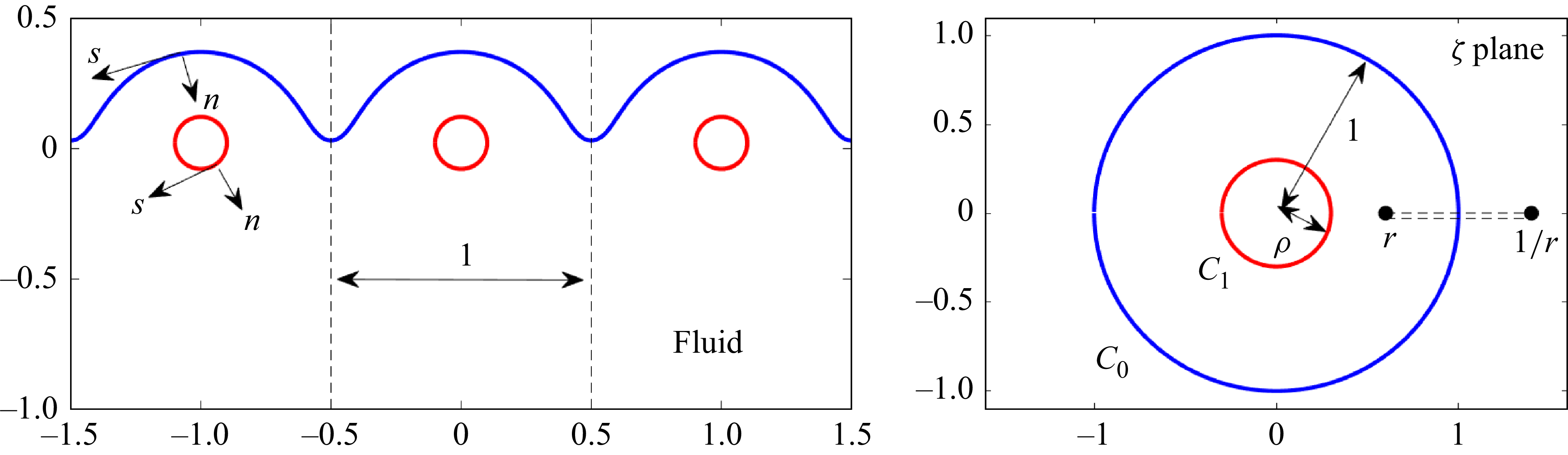


 Open access