


1. Introduction
Adding a tiny amount of high-molecular-weight polymer to a fluid dramatically reduces turbulent drag (Toms Reference Toms1949). Therefore, the polymer additives are used to reduce pumping costs in pipeline transport of crude oil and home heating and cooling systems, and to reduce fuel transfer time in airplane tank filling (Brostow Reference Brostow2008). Polymer additives also have been envisioned for flood remediation and enhancement of the drainage capacity of sewer systems (Sellin Reference Sellin1978; Bouchenafa et al. Reference Bouchenafa, Dewals, Lefevre and Mignot2021; Kumar & Graham Reference Kumar and Graham2023). Newtonian turbulent flow contains streamwise vortices close to walls, which dominate the near-wall momentum transport and, thus, the drag. During drag reduction, the polymer chains get stretched due to turbulence, leading to stress distributions that wrap around the streamwise vortices, weakening them to lead to lower turbulent drag (Kim et al. Reference Kim, Li, Sureshkumar, Balachandar and Adrian2007; Li & Graham Reference Li and Graham2007; Graham & Floryan Reference Graham and Floryan2021).
However, this suppression of near-wall vortices does not generally lead to full relaminarisation, but rather to a limiting state called the maximum drag reduction (MDR) asymptote. Some understanding of this observation has come from the discovery of elastoinertial turbulence (EIT), a complex chaotic flow that is sustained, rather than suppressed by viscoelasticity and, thus, helps explain the absence of relaminarisation (Samanta et al. Reference Samanta, Dubief, Holzner, Schäfer, Morozov, Wagner and Hof2013; Shekar et al. Reference Shekar, McMullen, Wang, McKeon and Graham2019; Dubief, Terrapon & Hof Reference Dubief, Terrapon and Hof2023). Nevertheless, the structure and mechanism underlying EIT remain poorly understood and are the topic of the present work.
EIT and MDR arise in parameter regimes of Reynolds number  $Re$ and Weissenberg number $\textit {Wi}$ (product of polymer relaxation time and nominal strain rate) where the unidirectional laminar flow is linearly stable and is thus a nonlinearly self-sustaining flow. The basic structure in both channel and pipe flows (Samanta et al. Reference Samanta, Dubief, Holzner, Schäfer, Morozov, Wagner and Hof2013; Lopez, Choueiri & Hof Reference Lopez, Choueiri and Hof2019) is two-dimensional (2-D) (Sid, Terrapon & Dubief Reference Sid, Terrapon and Dubief2018), characterised by vorticity fluctuations localised in narrow regions near the walls with tilted sheets of highly stretched polymers emanating from these regions. Figure 1 shows snapshots of velocity and polymeric stress fields of a simulated 2-D EIT in channel flow along with their temporal mean profiles in EIT and the corresponding profiles in the unidirectional laminar state.
Snapshots of perturbations of (a) wall-normal velocity ( $u_y'$), (b) streamwise velocity ( $u_x'$) and (c) trace of the polymer stress tensor ( $\mathrm {tr}(\boldsymbol {\tau }_{p}^{\prime })$) from their temporal arithmetic means in EIT. (d) Profiles of mean streamwise velocity ( $\bar {u}_x$) and mean of the trace of polymer stress tensor ( $\mathrm {tr}(\bar {\boldsymbol {\tau }}_{p})$) in EIT. (e) Profiles of streamwise velocity and the trace of the polymer stress tensor in the unidirectional laminar flow state. For all plots, $Re=3000$ and $\textit {Wi}=35$. The variables have been non-dimensionalised with their respective scales (see § 2).

Despite the absence of an obvious linear instability mechanism for EIT, it has been hypothesised that EIT is related to the nonlinear excitation of either a ‘wall mode’ or a ‘centre mode’ structure arising in the linear stability problem for the unidirectional laminar state (Drazin & Reid Reference Drazin and Reid1981; Datta et al. Reference Datta2022). A wall mode has a wave speed much less than the centreline velocity, and critical layer positions, i.e. where the wave speed equals the local laminar velocity, near the walls. In contrast, a centre mode travels at nearly the centreline velocity and accordingly the critical layer position is near the centreline. The Tollmien–Schlichting (TS) mode of classical linear analysis of plane Poiseuille flow is a wall mode, and there is a strong structural resemblance of the viscoelastic extension of the TS wave to EIT (Shekar et al. Reference Shekar, McMullen, Wang, McKeon and Graham2019, Reference Shekar, McMullen, McKeon and Graham2020, Reference Shekar, McMullen, McKeon and Graham2021). Figure 2 shows the viscoelastic linear TS mode under the same conditions as figure 1. Since the laminar state at these conditions is linearly stable, a sufficiently small random perturbation will decay, with the slowest mode of decay having this form. Sheets of highly stretched polymer are generated in the TS wave due to the presence of hyperbolic stagnation points (in the frame travelling with the wave) in the Kelvin cat's-eye structure of the velocity field in the critical layer (Shekar et al. Reference Shekar, McMullen, Wang, McKeon and Graham2019). The recently discovered ‘polymer diffusive instability’ (PDI) is also a wall mode (Beneitez, Page & Kerswell Reference Beneitez, Page and Kerswell2023; Couchman et al. Reference Couchman, Beneitez, Page and Kerswell2024). However, in the parameter regime considered in the present study, the PDI does not arise; the laminar profile is linearly stable, and accordingly simulations with initial conditions that are very small perturbations from laminar flow decay back to it. The possibility of a centre mode structure is of interest in part because there is a linear centre mode instability at low Reynolds number  $Re$ that may organise ‘elastic turbulence’ at very small Reynolds number $Re$ (Garg et al. Reference Garg, Chaudhary, Khalid, Shankar and Subramanian2018; Choueiri et al. Reference Choueiri, Lopez, Varshney, Sankar and Hof2021; Khalid et al. Reference Khalid, Chaudhary, Garg, Shankar and Subramanian2021; Morozov Reference Morozov2022). Nevertheless, in the elastoinertial regime considered here, although centre mode structures can exist (Dubief et al. Reference Dubief, Page, Kerswell, Terrapon and Steinberg2022), they do not appear to play an active role in the structure and self-sustenance of EIT (Beneitez et al. Reference Beneitez, Page, Dubief and Kerswell2024). The present work is consistent with this picture, and indeed deepens the connection between EIT and wall modes, showing in particular the existence of a nested family of such structures.
Structures of the perturbations of (a) wall-normal velocity ( $u_y'$), (b) streamwise velocity ( $u_x'$) and (c) trace of polymer stress tensor ( $\mathrm {tr}(\boldsymbol {\tau }_{p}^{\prime })$) from the unidirectional laminar state for the viscoelastic linear TS wave at $Re=3000$ and $Wi=35$. This mode ultimately vanishes as viscoelastic channel flow is linearly stable at this parameter regime.

In the present study, we investigate the structure and dynamics of EIT in channel flow using a modal decomposition technique known as spectral proper orthogonal decomposition (SPOD) (Towne, Schmidt & Colonius Reference Towne, Schmidt and Colonius2018). SPOD characterises coherent structures in complex flows that have well-defined structures and persist both in space and time via a frequency-domain variant of proper orthogonal decomposition (POD) (Lumley Reference Lumley1967). At a given frequency, SPOD generates an energetically ordered and spatially orthogonal set of modes characterising the flow. The modes and eigenvalues obtained using SPOD analysis can be interpreted as physical structures with a particular frequency and the energies associated with those structures (Schmidt & Towne Reference Schmidt and Towne2019). SPOD and dynamic mode decomposition (DMD) are related, as detailed in Towne et al. (Reference Towne, Schmidt and Colonius2018). In particular, DMD gives modes that correspond to particular frequencies. However, in DMD, there is no natural ordering of modes; in contrast, SPOD gives at each frequency an orthogonal basis set of modes ordered by their mean-square contribution to the flow at that frequency.
SPOD has been successfully used in inertial turbulence to understand coherent structures and develop a low-dimensional model for turbulence (Braud et al. Reference Braud, Heitz, Arroyo, Perret, Delville and Bonnet2004; Hellström & Smits Reference Hellström and Smits2014; Araya, Colonius & Dabiri Reference Araya, Colonius and Dabiri2017; Schmidt et al. Reference Schmidt, Towne, Colonius, Cavalieri, Jordan and Brès2017; Tutkun & George Reference Tutkun and George2017; Nekkanti & Schmidt Reference Nekkanti and Schmidt2021). Here, we use it to investigate travelling coherent structures underlying the chaotic dynamics of EIT. We focus on the frequency-dependence of the most energetic SPOD mode, as it reveals important coherent features of the flow.
2. Formulation and governing equations
Because the self-sustaining dynamics of EIT are fundamentally 2-D (Sid et al. Reference Sid, Terrapon and Dubief2018), we consider 2-D viscoelastic channel flow with non-dimensional equations of mass and momentum conservation:
 \begin{equation} \boldsymbol{\nabla}
\boldsymbol{\cdot} \boldsymbol{u}=0, \quad \frac{\partial
\boldsymbol{u}}{\partial
t}+\boldsymbol{u}\boldsymbol{\cdot} \boldsymbol{\nabla}
\boldsymbol{u} =-\boldsymbol{\nabla} p+\frac{\beta}{Re}
\nabla^2 \boldsymbol{u} + \frac{1-\beta}{Re}
\boldsymbol{\nabla} \boldsymbol{\cdot}
\boldsymbol{\tau}_p+f(t)\boldsymbol{e}_x,
\end{equation}
\begin{equation} \boldsymbol{\nabla}
\boldsymbol{\cdot} \boldsymbol{u}=0, \quad \frac{\partial
\boldsymbol{u}}{\partial
t}+\boldsymbol{u}\boldsymbol{\cdot} \boldsymbol{\nabla}
\boldsymbol{u} =-\boldsymbol{\nabla} p+\frac{\beta}{Re}
\nabla^2 \boldsymbol{u} + \frac{1-\beta}{Re}
\boldsymbol{\nabla} \boldsymbol{\cdot}
\boldsymbol{\tau}_p+f(t)\boldsymbol{e}_x,
\end{equation}
where  $\boldsymbol {u}$ and $p$ are non-dimensional velocity field and pressure field, respectively. Newtonian laminar centreline velocity ( $U_c$) and channel half-width ( $H$) have been used as characteristic velocity scale and length scale, respectively. The ratio between solvent viscosity ( $\eta _s$) to zero shear rate solution viscosity ( $\eta$) has been denoted by $\beta =\eta _s/\eta$. The Reynolds number has been defined as $Re=\rho U_c H/\eta$, where $\rho$ represents fluid density. We use no-slip boundary conditions for the velocity field at the channel wall. Periodic boundary conditions have been used at the inlet and outlet of the channel. Flow is driven by an external forcing term $f(t)\boldsymbol {e}_x$, where $\boldsymbol {e}_x$ denotes the streamwise direction. The forcing term varies with time to keep the bulk velocity ( $U_b=2U_c/3$) at its Newtonian laminar value. The polymer stress tensor is denoted $\boldsymbol {\tau }_p$ and we choose the FENE-P constitutive model with an artificial diffusion term to model its evolution:
 $$\begin{gather} \frac{\partial \boldsymbol{\alpha}}{\partial t}+\boldsymbol{u}\boldsymbol{\cdot} \boldsymbol{\nabla} \boldsymbol{\alpha} - \boldsymbol{\alpha}\boldsymbol{\cdot} \boldsymbol{\nabla} \boldsymbol{u}-(\boldsymbol{\alpha}\boldsymbol{\cdot} \boldsymbol{\nabla} \boldsymbol{u})^T=-\boldsymbol{\tau}_p+\frac{1}{Re \textit{Sc}} \nabla^2 \boldsymbol{\alpha}, \end{gather}$$
 $$\begin{gather}\boldsymbol{\tau}_p= \frac{1}{\textit{Wi}} \left( \frac{\boldsymbol{\alpha}}{1-\mathrm{tr}(\boldsymbol{\alpha})/b}-{\boldsymbol{\mathsf{I}}}\right), \end{gather}$$
where  $\boldsymbol {\alpha }$ is the conformation tensor and parameter $b$ characterises the maximum extensibility of the polymer chains. The polymer stress tensor is non-dimensionalised with $\eta U_c/H$. The Weissenberg number $\textit {Wi}=\lambda U_c/H$, where $\lambda$ is the polymer relaxation time. The Schmidt number $Sc=\eta /\rho D$, where $D$ is the diffusion coefficient, represents the ratio of momentum diffusivity to mass diffusivity. The artificial diffusion term is used to stabilise the numerical scheme during the integration of (2.2). The presence of this term leads to the requirement of boundary conditions for the conformation tensor. At the channel walls, we determine $\boldsymbol {\alpha }$ by solving the governing equations considering $Sc \to \infty$.
We solve the governing equations with a spectral method using the Dedalus framework (Burns et al. Reference Burns, Vasil, Oishi, Lecoanet and Brown2020). The computational domain has a length  $L=5$. The governing equations have been discretised using 256 Fourier basis functions and 1024 Chebyshev basis functions in the streamwise ( $x$) and wall-normal ( $y$) directions, respectively. We use $\beta =0.97$, $b=6400$, $Re=3000\unicode{x2013}6000$ and $\textit {Wi}=35\unicode{x2013}70$, which are relevant to turbulent drag reduction and are in the range of values used in previous studies (e.g. Shekar et al. Reference Shekar, McMullen, Wang, McKeon and Graham2019; Dubief et al. Reference Dubief, Page, Kerswell, Terrapon and Steinberg2022). In reality, the Schmidt number for a polymer solution is very large ( $Sc\sim 10^6$). Numerical simulation with such a large value of $Sc$ would require an extremely fine mesh and small time-step, making numerical simulations computationally very expensive. At the same time, small $Sc$ (i.e. $Sc<10$) smears out small-scale dynamics and suppresses EIT (Sid et al. Reference Sid, Terrapon and Dubief2018; Dubief et al. Reference Dubief, Terrapon and Hof2023). Therefore, numerical simulations of EIT based on artificial diffusion generally use $\textit {Sc}\sim O(100)$ (Sid et al. Reference Sid, Terrapon and Dubief2018; Buza et al. Reference Buza, Beneitez, Page and Kerswell2022). In the present study, we use $\textit {Sc}=250$ which is sufficient to sustain EIT and also numerically tractable. Viscoelastic channel flow in the parameter regime considered here is linearly stable. Therefore, to trigger EIT, we use unidirectional laminar flow with sufficiently large random perturbations in the conformation tensor as the initial condition of the simulation. In computing statistics, initial transients are dropped so that we consider only statistically stationary results.
To estimate the SPOD spectrum, the spatiotemporal state variables are organised in a vector  $\boldsymbol {q}(\boldsymbol {x},t)$. Here, we separately take this vector to contain wall-normal velocity, streamwise velocity or the trace of the polymer stress tensor, as further discussed in the following. For a statistically stationary flow, the SPOD analysis can be done in Fourier space, where $\tilde {\boldsymbol {q}}(\boldsymbol {x},f)$ denotes the Fourier-transformed dataset. Notation and methodology here follow Towne et al. (Reference Towne, Schmidt and Colonius2018). Given an inner product
 \begin{equation} \langle\boldsymbol{\tilde{q},\psi}\rangle= \int_{\varOmega} \boldsymbol{\psi}^*(\boldsymbol{x},f) \tilde{\boldsymbol{q}}(\boldsymbol{x},f)\, {\rm d}\boldsymbol{x}, \end{equation}
where  $(^*)$ denotes conjugate transpose, the SPOD seeks to find a function $\boldsymbol {\psi }(\boldsymbol {x},f)$ that maximises
 \begin{equation} E\{ | \langle \tilde{\boldsymbol{q}}(\boldsymbol{x},f), \boldsymbol{\psi}(\boldsymbol{x},f) \rangle |^2\}, \end{equation}
given the constraint  $\langle \boldsymbol {\psi }(\boldsymbol {x},f), \boldsymbol {\psi }(\boldsymbol {x},f) \rangle =1$, where $\boldsymbol {\psi }(\boldsymbol {x},f)$ is the SPOD mode at frequency $f$. The operators $E\{{\cdot }\}$ and $|{\cdot }|$ represent expectation and modulus, respectively. The maximisation of (2.5) leads to the following eigenvalue problem:
 \begin{equation} \int_{\varOmega} {\boldsymbol{\mathsf{S}}}(\boldsymbol{x,y},f) \boldsymbol{\psi}(\kern0.09em \boldsymbol{y},f) \,{\rm d}\boldsymbol{y}=\sigma (f) \boldsymbol{\psi}(\boldsymbol{x},f), \end{equation}
where the cross-spectral density (CSD) tensor  ${\boldsymbol{\mathsf{S}}}$ is
 \begin{equation} {\boldsymbol{\mathsf{S}}}(\boldsymbol{x,y},f) =E\{\tilde{\boldsymbol{q}}(\boldsymbol{x},f) \tilde{\boldsymbol{q}}^*(\kern0.09em \boldsymbol{y},f) \}. \end{equation}
This eigenvalue problem (2.6) leads to an infinite set of eigenmodes  $\{\sigma _j (f), \boldsymbol {\psi }_j(\boldsymbol {x},f)\}$ at each frequency, which are generally arranged in decreasing order of $\sigma _j$. These eigenvalues are often called ‘energies’, because in the case where the time series is velocity, each eigenvalue indicates the amount of kinetic energy associated with the associated mode. The eigenvectors ( $\boldsymbol {\psi }_j$) are orthogonal and provide a complete basis for $\tilde {\boldsymbol {q}}$. Therefore, the Fourier-transformed dataset at a given frequency can be written in terms of SPOD modes as
 \begin{equation} \tilde{\boldsymbol{q}}(\boldsymbol{x},f)= \sum_{j=1}^{\infty}a_j(f)\boldsymbol{\psi}_j(\boldsymbol{x},f), \end{equation}
where  $a_j(f)=\langle \tilde {\boldsymbol {q}}(\boldsymbol {x},f), \boldsymbol {\psi }_j(\boldsymbol {x},f) \rangle$ are the SPOD coefficients.
To calculate the SPOD of a discrete time series of  $N_t$ snapshots $\{\boldsymbol {q}(t_1),\boldsymbol {q}(t_2),\ldots,\boldsymbol {q}(t_{N_t})\}$, first, a data matrix ${\boldsymbol{\mathsf{Q}}}$ is constructed as
 \begin{equation} {\boldsymbol{\mathsf{Q}}}=[\boldsymbol{q}_1, \boldsymbol{q}_2,\ldots, \boldsymbol{q}_{N_t}], \end{equation}
where  $\boldsymbol {q}_i=\boldsymbol {q}(t_i)$. Multiple realisations of the flow field are generated by dividing the data matrix into overlapping blocks (Welch Reference Welch1967)
 \begin{equation} {\boldsymbol{\mathsf{Q}}}^n=[\boldsymbol{q}_1^n, \boldsymbol{q}_2^n, \ldots,\boldsymbol{q}_m^n,\ldots, \boldsymbol{q}_{N_f}^n], \quad n=1,2,\ldots, N_b, \end{equation}
where  $N_f$ is the number of snapshots in each block. The total number of blocks can be given as $N_b=(N_t-N_o)/(N_f-N_o)$, where $N_o$ represents the number of overlapping snapshots. The $m$th entry in the $n$th block ( $\boldsymbol {q}_m^n$) can be connected with the entry in ${\boldsymbol{\mathsf{Q}}}$ as $\boldsymbol {q}_m^n=\boldsymbol {q}_{m+(n-1)(N_f-N_o)}$. The non-periodicity of the data in each block may lead to spectral leakage during the estimation of the discrete Fourier transform (DFT). Therefore, to reduce the spectral leakage we compute the DFT of the windowed data:
 \begin{equation} {\boldsymbol{\mathsf{Q}}}^{n,w}=[w_1\boldsymbol{q}_1^n, w_2\boldsymbol{q}_2^n, \ldots,w_m\boldsymbol{q}_m^n,\ldots, w_{N_f}\boldsymbol{q}_{N_f}^n], \end{equation}
where  $w_m$ is the nodal value of the symmetric Hamming window function,
 \begin{equation} w_m= 0.54-0.46\cos \left(\frac{2{\rm \pi} (m-1)}{N_f-1} \right). \end{equation}
The DFT of  ${\boldsymbol{\mathsf{Q}}}^{n,w}$ gives
 \begin{equation} \tilde{{\boldsymbol{\mathsf{Q}}}}^n=[\tilde{\boldsymbol{q}}_1^n, \tilde{\boldsymbol{q}}_2^n, \ldots, \tilde{\boldsymbol{q}}_m^n,\ldots, \tilde{\boldsymbol{q}}_{N_f}^n], \end{equation}
where  $\tilde {\boldsymbol {q}}_m^n$ represents the Fourier component at frequency $f_m$ in the $n$th block. Next, the data matrix is organised frequency-wise, where the Fourier components at frequency $f_m$ from all the blocks are collected as
 \begin{equation} \tilde{{\boldsymbol{\mathsf{Q}}}}_m=[\tilde{\boldsymbol{q}}_m^1, \tilde{\boldsymbol{q}}_m^2,\ldots, \tilde{\boldsymbol{q}}_{m}^{N_b}]. \end{equation}
Now, the SPOD modes,  $\boldsymbol {\psi }_m$, and energies, $\boldsymbol {\sigma }_m$, at the frequency $f_m$ can be obtained by computing the eigenvectors and eigenvalues of the discretised CSD matrix ${\boldsymbol{\mathsf{S}}}_m=\tilde {{\boldsymbol{\mathsf{Q}}}}_m\tilde {{\boldsymbol{\mathsf{Q}}}}_m^*$ by solving the eigenvalue problem
 \begin{equation} {\boldsymbol{\mathsf{S}}}_m {\boldsymbol{\mathsf{W}}} \boldsymbol{\psi}_m = \boldsymbol{\psi}_m \boldsymbol{\sigma}_m, \end{equation}
where  ${\boldsymbol{\mathsf{W}}}$ is a positive-definite weighting matrix, which properly accounts for the numerical quadrature for integration on a non-uniform discrete grid, and $\boldsymbol {\sigma }_m$ is a diagonal matrix of eigenvalues. This equation is the discretised version of (2.6). In practice, the number of flow realisations ( $N_b$) is much smaller than the number of grid points. Therefore, for faster computation, the eigenvalue problem
 \begin{equation} \tilde{{\boldsymbol{\mathsf{Q}}}}_m^* {\boldsymbol{\mathsf{W}}} \tilde{{\boldsymbol{\mathsf{Q}}}}_m \boldsymbol{\varTheta}_m = \boldsymbol{\varTheta}_m \boldsymbol{\sigma}_m, \end{equation}
is solved. This has the same non-zero eigenvalues as (2.15), and its eigenvectors are related to those of (2.15) by the expression
 \begin{equation} \boldsymbol{\psi}_m = \tilde{{\boldsymbol{\mathsf{Q}}}}_m\boldsymbol{\varTheta}_m \boldsymbol{\sigma}_m^{-1/2}. \end{equation}
 For the SPOD analysis, we use the MATLAB tool developed by Schmidt (Reference Schmidt2022). Details of the method and its numerical implementation can be found in literature (Towne et al. Reference Towne, Schmidt and Colonius2018; Schmidt & Colonius Reference Schmidt and Colonius2020). We use  $600$ time units of data generated using EIT simulation to perform SPOD analysis, which is sufficient for the convergence of SPOD. The dataset consists of $N_t=8000$ snapshots, which are sampled at the interval of $\Delta t_s=0.075$ time units. In the present study, we use $N_f=500$ snapshots in each block with $50\,\%$ overlap ( $N_o=250$), which leads to a total of $N_b=31$ blocks. The SPOD spectra estimated using different combinations of $N_f$ and $N_o$ are presented in Appendix A. The number of modes obtained in SPOD is the same as the number of blocks, where the first mode has the highest energy and the last mode has the lowest energy. The number of non-negative frequencies is given by $N_f/2+1$ and the interval between discrete consecutive frequencies is $\Delta f= 1/ (\Delta t_s N_f)$.
3. Results and discussion
This study focuses on the case  $Re=3000, \textit {Wi}=35$, for which a snapshot of perturbation of wall-normal velocity $u_y'$, streamwise velocity $u_x'$ and the trace of the polymer stress tensor $\mathrm {tr}(\boldsymbol {\tau }_p')$ are shown in figure 1, where $(^{\prime })$ represents the perturbation from the temporal arithmetic mean. We have also plotted mean and laminar profiles of different state variables in figure 1. Note that the trace of the polymer stress field is closely related to the degree of polymer stretching, which is proportional to $\mathrm {tr}(\boldsymbol {\alpha })$. The dynamics of $u_y'$ in EIT are dominated by the downstream advection of large-scale structures spanning the channel (figure 1(a) and supplementary movie 1 available at https://doi.org/10.1017/jfm.2024.597) and the dynamics of $u_x'$ are dominated by the downstream advection of structures localised close to the channel walls (figure 1(b) and supplementary movie 2). The dynamics of the polymer stress field are dominated by the downstream motion of thin inclined sheets of polymer stress in the vicinity of the channel walls (figure 1(c) and supplementary movie 3). Since wall-normal velocity is identically zero in the laminar state, its temporal mean is also identically zero so it yields the cleanest Fourier and SPOD spectra. We note that the velocity fluctuations at EIT are generally quite small (e.g. $u_y'\sim 10^{-2}$ and drag is only $12.8\,\%$ higher than the laminar), so the streamwise velocity profile does not greatly differ from laminar and, hence, it remains the dominant component of velocity (figure 1). The trace of the polymer stress tensor represents the contribution of polymer chains in the stress field, which regulates the flow field. Therefore, $u_y'$, $u_x'$, $\mathrm {tr}(\boldsymbol {\tau }_p')$ are the important variables to be analysed using SPOD.
We perform SPOD analyses of the perturbation fields  $u_y'$, $u_x'$, and $\mathrm {tr}(\boldsymbol {\tau }_{p}^{\prime })$ separately due to the intense memory requirements of the algorithm of Schmidt (Reference Schmidt2022). However, for a small dataset ( $N_t=4000, N_o=125$), we have also calculated the SPOD spectrum of the velocity components together, which shows that the main characteristics of SPOD spectra remain unchanged (Appendix B). As we show, the spectral characteristics arising from each separate analysis are highly consistent, displaying peaks at the same frequencies. It is possible in principle, though highly memory intensive, to perform SPOD on the entire velocity and stress (or conformation) field, by extending the framework presented for POD by Wang et al. (Reference Wang, Graham, Hahn and Xi2014). As indicated there, as well as in Hameduddin & Zaki (Reference Hameduddin and Zaki2019), some subtleties arise in working with tensors such as $\boldsymbol {\alpha }$ that are constrained to be positive definite.
SPOD eigenvalue spectra as a function of frequency for the first several modes in  $u_y'$, $u_x^{\prime }$ and $\mathrm {tr}(\boldsymbol {\tau }_{p}^{\prime })$ are shown in figures 3(a), 3(b) and 3(c), respectively, along with the sum of eigenvalues of all the modes. For velocity components, the eigenvalue represents the kinetic energy as mentioned earlier and the total kinetic energy can be represented by the SPOD amplitude as $\|\boldsymbol{a}\|^2$ (2.8). The leading modes in wall-normal velocity and streamwise velocity contain most of the energy ( $\approx 73\,\%$ and $\approx 55\,\%$, respectively) and, hence, dominate the flow structure (figure 3(a,b)). In the eigenvalue spectrum of $\mathrm {tr}(\boldsymbol {\tau }_{p}^{\prime })$, the leading mode has a relatively smaller contribution ( $\approx 31\,\%$) to $\|\boldsymbol{a}\|^2$ (figure 3c). The leading modes of wall-normal velocity and streamwise velocity contain distinct sharp peaks at specific frequencies, of which the first few are indicated with red symbols, and the energy of these peaks decreases as the frequency increases. The leading mode of the polymer stress field also has peaks at the same frequencies; they are not as sharp as the peaks for the velocity components but still quite distinct, as revealed by plotting on a linear scale (inset). The higher-order modes do not have such distinct peaks. The energy decay of velocity fluctuations in the SPOD spectra at a large frequency ( $\,f>1$) approximately follows a ‘power law’ $f^{-5.2}$, which is somewhat close to the result $f^{-14/3}$ reported by Dubief, Terrapon & Soria (Reference Dubief, Terrapon and Soria2013). The SPOD spectrum of $\mathrm {tr}(\boldsymbol {\tau }_{p}^{\prime })$ follows a different power law ( $\,f^{-3.4}$). The significance of these is unclear as they are only observed over less than a decade in frequency; we report them here only for completeness.
SPOD eigenvalue spectra of perturbations of (a) wall-normal velocity ( $u_y'$), (b) streamwise velocity ( $u_x^{\prime }$) and (c) trace of polymer stress tensor ( $\mathrm {tr}(\boldsymbol {\tau }_{p}^{\prime })$) at $Re=3000$ and $\textit {Wi}=35$. Red symbols indicate the first few peaks in the leading mode of the eigenvalue spectra. Insets: SPOD eigenvalue spectra of the leading SPOD modes on a linear scale.

The local peaks in the energy spectrum of velocity components indicate that the structures corresponding to these frequencies have distinct features in the dynamics of EIT. These peaks are not at integer multiples of the lowest-frequency peak, so are not simply harmonics; the relationship between them is elucidated in the following. The SPOD mode structures of  $u_y'$, $u_x^{\prime }$, and $\mathrm {tr}(\boldsymbol {\tau }_{p}^{\prime })$ corresponding to the peak frequencies in the leading SPOD mode have been shown in figure 4. Each mode structure has a distinct wavenumber $\kappa$, which we measure in wavelengths per domain length. These modes are all travelling waves with wave speed $C_w=fL/\kappa$, as further discussed in the following.
Structures of SPOD modes of (a–e)  $u_y'$, (f–j) $u_x^{\prime }$ and (k–o) $\mathrm {tr}(\boldsymbol {\tau }_{p}^{\prime })$ at $Re=3000$ and $\textit {Wi}=35$, i.e. corresponding to the frequencies denoted by different symbols in the eigenvalue spectra (figure 3a–c).

The most dominant SPOD structure ( $\,f=0.08$) has unit wavenumber ( $\kappa =1$). The wall-normal velocity component for this mode consists of large-scale structures spanning the channel (figure 4a), the streamwise velocity component has regions of positive and negative velocity fluctuations close to the walls (figure 4f), and the polymer stress field displays thin layers close to the walls having inclined alternating sheets of positive and negative stress fluctuations (figure 4k). The structures approximately obey a shift–reflect symmetry: i.e. $u_y'(x,y)\approx -u_y'(x+L/2, -y)$, $u_x^{\prime }(x,y)\approx u_x^{\prime }(x+L/2, -y)$ and $\mathrm {tr}(\boldsymbol {\tau }_{p}^{\prime })(x,y) \approx \mathrm {tr}(\boldsymbol {\tau }_{p}^{\prime })(x+L/2,-y)$. The quantification of the shift–reflect symmetry of different SPOD mode structures is given in Appendix C. This is the symmetry obeyed by the TS mode (Drazin & Reid Reference Drazin and Reid1981), and comparison to figure 2 indicates a strong similarity in structure. From here onwards, we refer to the regions having positive and negative $u_y'$ as ‘positive lobe’ and ‘negative lobe’, respectively. The mode structures corresponding to other peaks have similar structures, where the wavenumber of structures increases with frequency (figure 4). The wall-normal extent of the lobes in $u_y'$ decreases and the regions of velocity fluctuations in $u_x^{\prime }$ approach the centreline of the channel as the wavenumber increases. Relatedly, the layers of strong $\mathrm {tr}(\boldsymbol {\tau }_{p}^{\prime })$ move away from the wall as the frequency increases.
The wave speeds of the travelling structures in the leading SPOD mode are shown in figure 5. They initially increase with the wavenumber (and frequency) and ultimately approach a value close to the centreline velocity of the channel ( $C_w \to 0.94$). The wave speed of the dominant mode structure ( $\,f=0.08,\kappa =1$) is very close to that of the Newtonian nonlinear TS (NNTS) wave at the corresponding $Re$ ( $C_{TS}=0.42$), shown in red in figure 5, further strengthening the evidence connecting EIT to the TS mode. The NNTS wave belongs to the stable (in two dimensions) upper branch of the nonlinear travelling wave solution of plane Poiseuille flow, which originates at $Re=5772$ through a subcritical bifurcation from the laminar branch and exists down to $Re \approx 2800$ (Jiménez Reference Jiménez1990; Shekar et al. Reference Shekar, McMullen, McKeon and Graham2020). By contrast, a centre mode would have a wave speed close to unity and, thus, a frequency close to $\kappa /L$. For $L=5$ this would be multiples of $0.2$, and figure 3(a) shows no peaks at these positions. In fact, $f=0.2$ and its multiples are close to local minima in energy for the dominant SPOD mode. In short, we see no evidence of a centre mode structure. The origin of the peak positions in figure 3(a) is elucidated in the following.


As discussed in the introduction, corresponding to the wave speed of a perturbation there is a critical layer position  $y_c$. As this is the position where the fluid and the perturbation are moving together, it is the most favourable position for the two to exchange energy. The velocity fluctuations in EIT are very weak so we can approximate the local streamwise velocity with the laminar value, $u_x\approx 1-y^2$, and the location of critical layers (i.e. where $C_w=u_x$) can be given as $y_c\approx \pm \sqrt {1-C_w}$. Figure 5 shows the critical layer positions corresponding to the wave speeds of the travelling structures of the leading SPOD mode, as well as for the NNTS mode. As with wave speed, the critical layer position of the $f=0.08, \kappa =1$ SPOD mode is very close to that of the NNTS mode.
To illustrate the relation between the critical layer and the location of the peaks in the SPOD stress fluctuation structures, in figure 6 we plot the positions of the critical layers for the travelling structures of the leading SPOD mode at the first several peak frequencies, along with the wall-normal distribution of polymer stress fluctuations ( $P(\kern0.09em y)$), which has been defined as
 \begin{equation} P(\kern0.09em y)=\left[ \frac{\displaystyle\int_0^L \{\mathrm{tr}(\boldsymbol{\tau}_p^{\prime})\}^2 \,{{\rm d}\kern0.06em x}}{\displaystyle\int_{-1}^1 \int_0^L \{\mathrm{tr}(\boldsymbol{\tau}_p^{\prime})\}^2 \,{{\rm d}\kern0.06em x}\, {{\rm d} y}}\right]^{1/2}.\end{equation}
The peak regions in  $P(\kern0.09em y)$ represent the locations of the sheets of polymer stress fluctuations, and we see that their locations correspond to the critical layers. A similar observation has been made for viscoelasticity-modified TS waves and it has been reported that thin sheets of high polymer stress emanate from the critical layers of TS waves (Hameduddin, Gayme & Zaki Reference Hameduddin, Gayme and Zaki2019; Shekar et al. Reference Shekar, McMullen, Wang, McKeon and Graham2019).
Wall-normal distribution of polymer stress fluctuations  $P(\kern0.09em y)$ (solid lines) and the positions of critical layers (dashed lines) for travelling modes having wave speed $C_w=0.4$ (black), $C_w=0.73$ (green), $C_w=0.84$ (blue) and $C_w=0.9$ (red) at $Re=3000$ and $\textit {Wi}=35$.

We noted previously that as the wavenumber increases,  $u_y'$ becomes more localised towards the channel centre, as do the critical layer positions where the stress fluctuations are high. More specifically, consider the $u_y'$ profile at the second peak ( $\,f=0.29$, figure 4b) and the $\mathrm {tr}(\boldsymbol {\tau }_p^{\prime })$ profile at the first peak ( $\,f=0.08$, figure 4k). It appears that the ‘lobes’ where $u_y'$ is large in the former figure are roughly bounded by the layers where
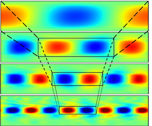
  $\mathrm {tr}(\boldsymbol {\tau }_p^{\prime })$ is large in the latter. Similar observations can be made about all of the succeeding modes. We visualise this point in figure 7, which replots the results of figure 4 by showing contour lines of $u_y'$ from the SPOD modes at wavenumber $\kappa +1$ juxtaposed with colour contours of $\mathrm {tr}(\boldsymbol {\tau }_p^{\prime })$ at wavenumber $\kappa$. From this figure, we see that the velocity lobes at wavenumber $\kappa +1$ are ‘nested’ within the stress fluctuations or, equivalently, between the upper and lower critical layer positions at wavenumber $\kappa$. In contrast, the regions between the critical layers and the channel walls contain small-scale and irregular structures both in the velocity field as well as stress field.
Contours of velocity fluctuations ( $u_y'$) of a faster-travelling wave on the top of the stress fluctuations of the immediate slower travelling wave: (a) stress at $C_w=0.4$ and velocity at $C_w=0.73$, (b) stress at $C_w=0.73$ and velocity at $C_w=0.84$, (c) stress at $C_w=0.84$ and velocity at $C_w=0.9$ and (d) stress at $C_w=0.9$ and velocity at $C_w=0.93$. Other parameters are $Re=3000$ and $\textit {Wi}=35$.

We now present a simple theory for the results in figure 5 that is motivated by the previous structural observations. The nested nature of the structures revealed by SPOD suggests that the locations of the polymer sheets of a slow-moving (low-wavenumber) travelling wave act like ‘walls’ for the immediately faster-moving (and higher-wavenumber) wave. Consider the existence of a ‘primary’ mode with wave speed  $C_{w,1}$ and, thus, critical layer positions $y_{c,1}=\pm (1-C_{w,1})^{1/2}$. We take the next higher mode to occupy the domain $|y|<| y_{c,1}|$; if its critical layer position $y_{c,2}$ is at the same fractional position in this new domain, it will thus be at $\pm |y_{c,1}|^2= \pm (1-C_{w,1})^{1}$. Continuing in this way, and noting that successively higher-speed waves can be labelled by their wavenumber $\kappa$, we have a simple scaling result
 \begin{equation} y_{c,\kappa}=(1-C_{w,1})^{\kappa/2}.\end{equation}
Relatedly, the successive wave speeds are then
 \begin{equation} C_{w, \kappa}=1-(1-C_{w,1})^{\kappa}.\end{equation}
Using the SPOD results for  $y_{c,\kappa }$ to find a best-fit value of $C_{w,1}$ yields predictions for $y_{c,\kappa }$ and $C_{w,\kappa }$ that agree very closely with the data, as shown in figure 5. Furthermore, the value of $C_{w,1}=0.44$ is very close to the NNTS wave speed $C_{TS}=0.42$. These observations indicate that the structure of EIT is dominated by nested self-similar structures that closely resemble TS waves.
Finally, we briefly hypothesise a possible physical mechanism for the appearance of this nested structure. A highly stretched elastic sheet resists lateral deformation. Similarly, flows in which polymer molecules are strongly stretched along one direction resist deformations transverse to that direction. A classical example of this mechanism is the suppression of shear-layer instability in a viscoelastic fluid, where the strong stretching in the shear layer mimics an elastic sheet (Azaiez & Homsy Reference Azaiez and Homsy2006). Relatedly, viscoelastic Taylor–Couette instability is suppressed by the normal stress induced by axial flow (Graham Reference Graham1998), and in porous media flows, sheetlike regions with high polymer stress resist the flow passing through them and, hence, act like flow barriers (Kumar, Guasto & Ardekani Reference Kumar, Guasto and Ardekani2023).
A similar mechanism may be at work here, in which the sheets of high polymer stress in the critical layers from the primary mode prevent velocity fluctuations from the higher modes from passing through the critical layer, acting as ‘walls’ as noted previously, and so on successively with the higher modes, leading to the emergence of a nested family of travelling waves. The resemblance of the SPOD mode structure in the reconstructed polymer stress field can be seen in Appendix D. Regardless of the detailed physical mechanism, the excellent agreement between the simulation results and the scaling theory manifested in (3.2) and (3.3) indicates the predictive power of the simple structural picture of nested travelling waves with critical layer fluctuations that define the length scale of the nesting.
For completeness, we also report in figure 8 the structures corresponding to the second-most energetic mode from SPOD (blue curves on figure 3) at  $f=0.08$. Note that the energy of this mode is substantially smaller than that of the leading mode and that the spectrum of this structure does not contain distinct peaks. This mode also has $\kappa =1$ and, thus, the same wave speed and critical layer position as the most energetic mode. It again exhibits localised polymer stretch fluctuations in the critical layer, but now displays simple reflection symmetry rather than the shift–reflect symmetry of the dominant mode. We view this as a higher-order correction on the dominant structure elucidated previously.
Mode structures of the second-most-energetic mode at  $f=0.08$; (a) $u_y'$, (b) $u_x'$ and (c) $\mathrm {tr}(\boldsymbol {\tau }_{p}^{\prime })$. Other parameters are $Re=3000$ and $\textit {Wi}=35$.

Results obtained for  $(Re=3000, \textit {Wi}=70)$ and $(Re=6000, \textit {Wi}=35)$ display nearly identical features to the case considered previously ( $Re=3000, \textit {Wi}=35$). The leading modes of the SPOD energy spectra of $u_y'$ at different $\textit {Wi}$ and $Re$ have been shown in figures 9(a) and 9(b), respectively. The SPOD spectra of other state variables have peaks exactly at the same frequencies as the spectrum of $u_y'$. Hence, they do not provide any additional information. As $\textit {Wi}$ increases, the region close to the first peak in the SPOD spectrum becomes slightly flatter. We do not see any significant effect of $\textit {Wi}$ on the peak frequencies in the SPOD spectra, which suggests that $\textit {Wi}$ does not have any noticeable impact on the qualitative nature of the travelling structures. As $Re$ increases, the mode energy corresponding to the lower-wavenumber peaks decreases, whereas the energy corresponding to the higher-wavenumber peaks increases. However, the frequencies corresponding to the peaks in the SPOD spectra remain unchanged indicating that the speed of the travelling wave is independent of $Re$. We also plot the SPOD mode structures of $u_y'$, $u_x'$, and $\mathrm {tr}(\boldsymbol {\tau }_{p}^{\prime })$ at the frequencies corresponding to the peaks in the leading SPOD mode at $Re=6000$ (figure 10). The mode structures of the travelling waves at $Re=6000$ are qualitatively similar to the structures at $Re=3000$ (figure 4).
Leading modes of SPOD energy spectra of  $u_y'$ at different (a) $\textit {Wi}$ at $Re=3000$ and (b) $Re$ at $\textit {Wi}=35$.

Structures of SPOD modes of (a–e)  $u_y'$, (f–j) $u_x'$ and (k–o) $\mathrm {tr}(\boldsymbol {\tau }_{p}^{\prime })$ at the peak frequencies in the leading mode of $u_y'$ at $Re=6000$ and $\textit {Wi}=35$.

At  $Re$ relevant to the present study, EIT overwhelmingly represents the MDR state (Lopez et al. Reference Lopez, Choueiri and Hof2019). Hence, the self-sustaining chaotic nature of the MDR state and its dynamics can be explained by the EIT. As noted earlier, the dynamics of EIT in both three-dimensional (3-D) channel and pipe flows are fundamentally 2-D (Sid et al. Reference Sid, Terrapon and Dubief2018; Lopez et al. Reference Lopez, Choueiri and Hof2019); specifically, 2-D finite-amplitude perturbations are self-sustaining. Therefore, it is expected, and observed (Shekar et al. Reference Shekar, McMullen, Wang, McKeon and Graham2019), that EIT even in 3-D flows would contain travelling waves originating from wall modes similar to the 2-D channel flow considered in the present study. At larger $Re$, the MDR state may not be fully dominated by 2-D EIT, and 3-D flow structures may arise in that scenario. An important direction for future work will be to apply SPOD to the full 3-D case.
4. Conclusions
In the present study, we have used SPOD to elucidate the structure underlying the chaotic dynamics of 2-D EIT in channel flow. The most energetic mode of SPOD spectrum has distinct peaks. The mode structures corresponding to these peaks exhibit a family of well-defined travelling structures, where the velocity field contains large-scale regular patterns and the polymer stress field contains the formation of thin inclined sheets of high and low stress at the critical layers of the wave. The structure of the most dominant travelling wave (first mode, highest peak) of this family exhibits shift–reflect symmetry and resembles the structure of the TS wave indicating its origin in a nonlinearly self-sustained wall mode. The travelling structures corresponding to the higher frequency peaks have very similar structure and symmetry, however, their wavenumber increases, and the size of large-scale structures decreases. It appears that the localised polymer sheets at the critical layers of the leading SPOD mode at a given peak frequency act like walls for the travelling structure of the mode corresponding to the next peak and, hence, lead to a nested arrangement of the waves. Based on this observation, a simple theory quantitatively captures the relationship between the wave speeds and the locations of critical layers for different waves. From this analysis, a picture emerges of 2-D EIT as a nested collection of nonlinearly self-sustaining TS-wave-like structures.
Supplementary movies
Supplementary movies are available at https://doi.org/10.1017/jfm.2024.597.
Acknowledgements
We are grateful to A. Towne for helpful discussions and Oliver Schmidt for making available his SPOD code.
Funding
This research was supported under grant ONR N00014-18-1-2865 (Vannevar Bush Faculty Fellowship).
Declaration of interests
The authors report no conflict of interest.
Appendix A. Effect of block size and overlap on SPOD spectra
To investigate the effect of the block size ( $N_f$) and overlap on the estimation of SPOD spectra, we plot the SPOD spectra of $u_y'$ obtained using different block sizes and overlaps (figure 11). We do not see any noticeable difference between the peaks in the SPOD spectra obtained using $N_f=500$ with $50\,\%$ overlap in the main text (figure 3a) and the spectra obtained using different combinations of $N_f$ and overlap (figure 11).
SPOD energy spectra of  $u_y'$ at $Re=3000$ and $\textit {Wi}=35$ estimated using (a) block size $N_f=500$ with $25\,\%$ overlap, (b) block size $N_f=500$ with $75\,\%$ overlap and (c) block size $N_f=1000$ with $50\,\%$ overlap.

Appendix B. SPOD estimation of velocity components together
For a small dataset ( $N_t=4000$) and lower overlap ( $25\,\%$), we have calculated the SPOD spectrum of velocity components altogether (figure 12). The peaks in the leading mode are exactly at the same frequencies as the SPOD calculated for each velocity component separately (figure 3a,b).
SPOD energy spectrum of the velocity field ( $u_x'$ and $u_y'$ together) at $Re=3000$ and $\textit {Wi}=35$ estimated using $N_t=4000$ with $25\,\%$ overlap.

Appendix C. Quantification of the symmetry of SPOD mode structures
To quantify the shift–reflect symmetry of the SPOD mode structures, we define a parameter  $R$ as
 \begin{equation} R=\frac{\|A(x,y) - B(x,y)\|^2}{4\|A(x,y)\|^2}, \end{equation}
where  $A(x,y)$ represents SPOD structures ( $u_y'$, $u_x^{\prime }$ and $\mathrm {tr}(\boldsymbol {\tau }_{p}^{\prime })$) and $B(x,y)$ represents their shift–reflect image. Here $R=0$ and $R=1$ represent perfect shift–reflect symmetry and reflect symmetry, respectively. The small values of $R$ confirm that the SPOD structures obey shift–reflect symmetry (table 1). The value of $R$ for $\mathrm {tr}(\boldsymbol {\tau }_{p}^{\prime })$ is relatively larger than $u_y'$, because the SPOD modes of $\mathrm {tr}(\boldsymbol {\tau }_{p}^{\prime })$ are characterised by thin sheets and even a slight misalignment between sheets leads to a larger value of $R$.
$R$.
Values of shift–reflect symmetry parameter  $R$ (C1) for SPOD of various quantities and modes.

Appendix D. Reconstruction of polymer stress field using specific SPOD mode
To visualise the signature of the SPOD structure in the polymer stress field, we plot the reconstruction of the polymer stress field just using the most dominant SPOD mode (first mode, highest peak) (figure 13). In the reconstructed stress field, we see the existence of thin sheets characterised by large polymer stress.
Reconstruction of  $\mathrm {tr}(\boldsymbol {\tau }_{p})$ just using the most dominant SPOD mode (first mode, highest peak) at $Re=3000$ and $Wi=35$.


 Open access