


Introduction
Numerical models have been instrumental in understanding the stratigraphic paleobiology of marine systems, that is, how the structure of the stratigraphic record controls the expression of the fossil record (Holland Reference Holland1995, Reference Holland, Erwin and Wing2000, Reference Holland2020; Holland and Patzkowsky Reference Holland and Patzkowsky1999, Reference Holland and Patzkowsky2002, Reference Holland and Patzkowsky2015). These models have served as a baseline for understanding the stratigraphic expression of mass extinctions and recoveries (Nawrot et al. Reference Nawrot, Scarponi, Azzarone, Dexter, Kusnerik, Wittmer, Amorosi and Kowalewski2018; Zimmt et al. Reference Zimmt, Holland, Finnegan and Marshall2020), diachroneity of range end points (Holland and Patzkowsky Reference Holland and Patzkowsky1999), and the tempo of ecological change and patterns of morphological change (Webber and Hunda Reference Webber and Hunda2007). These models also guide the sampling of the fossil record, so that evolutionary and ecological patterns can be distinguished from patterns that have a stratigraphic origin (Patzkowsky and Holland Reference Patzkowsky and Holland2007; Ivany et al. Reference Ivany, Brett, Wall, Wall and Handley2009). Even where these models fail to capture all aspects of the fossil record, as is true for any model, they indicate where additional considerations must be included, such as changes in fossil abundance (Nawrot et al. Reference Nawrot, Scarponi, Azzarone, Dexter, Kusnerik, Wittmer, Amorosi and Kowalewski2018).
Similar models for the nonmarine fossil record have not been developed, and they have long been needed (Patzkowsky and Holland Reference Patzkowsky and Holland2012). In particular, an understanding of the controls on large-scale patterns in the ratio of channel facies to floodplain facies would be useful, because numerous studies have shown how this controls the taphonomy and composition of the nonmarine fossil record (Bown and Kraus Reference Bown and Kraus1981; Behrensmeyer and Hook Reference Behrensmeyer, Hook, Behrensmeyer, Damuth, DiMichele, Potts, Sues and Wing1992; Badgley and Behrensmeyer Reference Badgley and Behrensmeyer1995; Rogers and Kidwell Reference Rogers and Kidwell2000; Gastaldo and Demko Reference Gastaldo and Demko2011; Lyson and Longrich Reference Lyson and Longrich2011; and many others, including a recent review in Holland and Loughney Reference Holland and Loughney2021). Here, I describe a coupled stratigraphic–biologic model for the assembly of the nonmarine fossil record. This coupled model is used to propose a series of testable hypotheses for the structure of the nonmarine fossil record relative to sequence-stratigraphic architecture over timescales of hundreds of thousands to a few tens of millions of years.
Model
The model presented here combines two threads, one stratigraphic and one biologic. The stratigraphic thread begins with a two-dimensional geometric model for simulating changes in a fluvial depositional profile through time, and therefore the accumulation and erosion of nonmarine sediment. This allows the simulation of stratigraphic columns in the nonmarine portion of the sedimentary basin. The biologic thread includes a random-branching model for simulating species evolution, along with an ecological model for describing species distribution along an environmental gradient correlated with elevation relative to sea level. The results of these two threads are combined to simulate the occurrence of species through stratigraphic columns under a variety of stratigraphic architectures.
The coupled model is divided into several components, which fosters testability and reuse. Full source code in R (v. 4.1.0; R Core Team 2021), example workflows, and the model parameters of each simulation presented here are available in a Zenodo Data Repository. Models simulate a 500-km cross section oriented along depositional dip, and the time covered by the simulations varies from 3.0 to 7.0 Myr, with a temporal resolution of 10 Kyr.
Basin-Scale Model
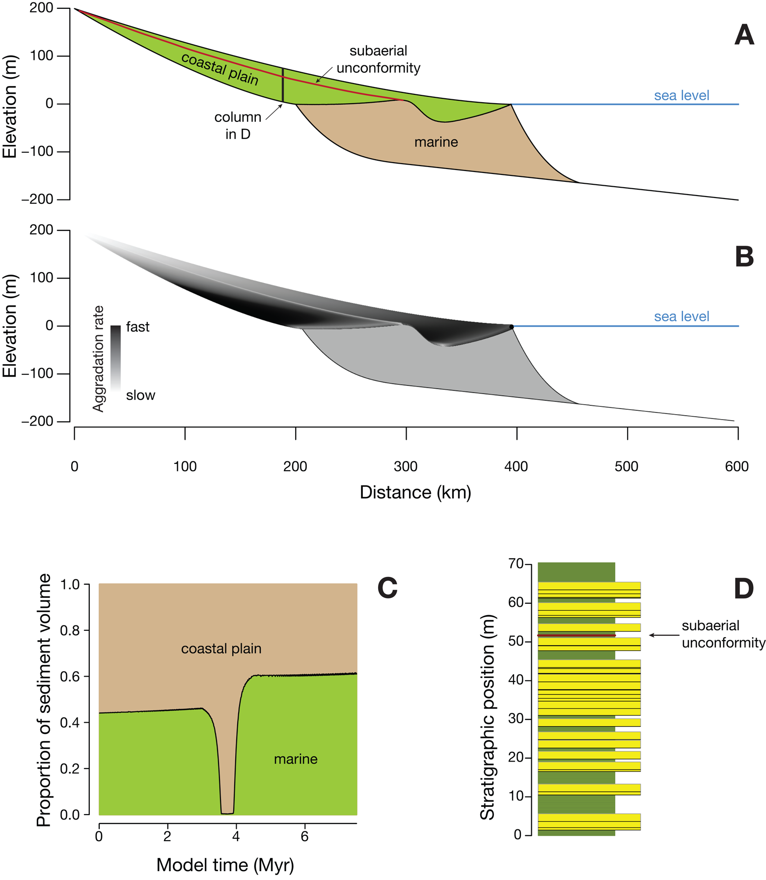
The sedimentary basin is simulated using a geometric approach, in which the nonmarine coastal plain and marine areas are each simulated as conforming to a concave equilibrium profile (Holland and Loughney Reference Holland and Loughney2021; Fig. 1A). A geometric model simulates sedimentation by preserving the geometry (here, concave equilibrium profiles), in contrast to a process-based model, which simulates sedimentation by the physics of sediment transport. Concave profiles have commonly been simulated with diffusion and exponential functions (e.g., Jordan and Flemings Reference Jordan and Flemings1991), but Caputo curves provide a better fit to river profiles (Voller and Paola Reference Voller and Paola2010). Studies that have fit diffusion profiles to nonmarine and marine systems have found that marine profiles are generally steeper and more concave, and that difference is followed here (Jordan and Flemings Reference Jordan and Flemings1991). The exact form of these concave curves has a negligible effect on the results of the model, and straight profiles produce similar outcomes.
A, Topographic profile through simulated basin with gently concave coastal plain profile and more strongly concave marine profile. Coastal plain profile connects the fall line (the inland edge of the sedimentary basin) to the shore, and the marine profile connects the shore to the toe of the marine profile, with an initially flat shelf beyond. B, Accumulation of sediment (gray) as a result of sea-level rise. Volume of sediment is held constant, and optimal position of the shore is found with the constraints that the fall line is fixed in place, and the toe of the marine profile is a fixed distance seaward of the shore. C, Erosion (vertical hatching) and accumulation of sediment (gray) as a result of sea-level fall. After the fall in sea level, the equilibrium nonmarine profile lies along on the dashed line in the valley, but it lies along the solid line above that on the interfluve, as it is a non-erosive hiatal surface.

Both profiles are anchored at their end points. The nonmarine profile is anchored upstream at the fall line, which marks the landward edge of the depositional basin, and it is anchored downstream at the shore. The marine profile is anchored on its landward side at the shore and at its toe on its seaward side. The toe of the marine profile is set at a fixed distance from the shore, within the range of modern deltas (Elliott Reference Elliott and Reading1986).
The model proceeds in a series of time steps of fixed length (all model parameters are listed in the Supplementary Material). In each time step, the basin is allowed to subside, eustatic sea level may change, and then sediment is deposited. The model records the amount of sediment accumulated and the elevation everywhere in the basin at every time step. Throughout this article, “elevation” is used to refer to the elevation relative to sea level of any point on the landscape at the time of deposition. This is in contrast with “stratigraphic position,” which refers to the height of a sedimentary horizon within a stratigraphic column. The basin model contains no information on sedimentary environments, such as channels or floodplains, which are incorporated at a later stage in the stratigraphic-column model (see “Stratigraphic-Column Model”).
Although the basin model can handle a range of spatial and temporal variations in subsidence, subsidence is treated in these simulations as a hinge with zero subsidence at the fall line, with linearly increasing subsidence rates toward the distal (right) edge of the basin. This mimics the subsidence pattern found on passive margins, intracratonic basins, and the distal edge of foreland basins, among others (Allen and Allen Reference Allen and Allen2005). Subsidence rates are held constant through time. The construction of the model will ultimately make it possible to simulate the proximal side of foreland basins in which subsidence is greatest at the landward edge. Eustasy is varied in the simulations as described in “Results.”
Sedimentation is accomplished by assuming that a fixed amount of sediment enters the basin at each time step (Fig. 1), although the model can simulate temporally variable sediment flux. Sedimentation is handled by simultaneously satisfying seven constraints: the vertical and lateral position of the fall line is fixed, the nonmarine and marine profiles follow a Caputo curve with fixed parameters, the marine profile has a fixed width relative to the position of the shore, the toe of the marine profile is pinned to the seafloor, and the volume of sediment is fixed. This leaves one free parameter, the lateral position of the shore along the plane defined by sea level. This lateral position of the shore is found through optimization, placing it where the specified fixed volume of sediment is achieved. This approach of conserving sediment volume produces a sedimentary record that is balanced, like the model of Jervey (Reference Jervey1988), which was instrumental in establishing the principles of sequence stratigraphy. The crucial difference in the model presented here is that the coastal plain is simulated as concave rather than horizontal and flat.
A relative rise in sea level promotes the aggradation of sediment along one or both profiles (Fig. 1B), but a relative fall in sea level may cause the new nonmarine profile to lie below the old land surface (Fig. 1C). This creates erosion within a valley, that is, a topographic low much broader and wider than a single river channel (Shanley and McCabe Reference Shanley and McCabe1994). The creation of a valley also produces interfluves, relatively flat and topographically high areas between valleys. Interfluves are starved of sediment, because the river lies well below the elevation of the interfluve, and in actual geological situations, they are sites of the formation of mature, well-drained paleosols.
Because relative sea-level fall can cause the new depositional surface to lie below the former depositional surface, the model simulates two cases, one along the valley and another along the interfluve. Along the valley, erosion lowers the land surface down to the new equilibrium surface, and it is along this valley profile that sediment volume is calculated. Because the amount of sediment eroded in the valley is minor compared with the sediment supplied to the basin (Blum and Tornqvist Reference Blum and Tornqvist2002), the additional sediment supplied by valley erosion is ignored. Along the interfluve, erosion does not take place, causing the land surface to become perched above the equilibrium profile (Fig. 1C), and it therefore receives no sediment for as long as it lies above the equilibrium profile.
Stratigraphic-Column Model
Stratigraphic columns are built such that each reflects the accumulation of sediment through time at a particular location in the basin model. In marine areas, the thickness of accumulated marine sediment is given by the basin model, but it is recorded without specific facies information, as this model is focused on the nonmarine record. In nonmarine areas, the stratigraphic column simulates two cases: deposition on the floodplain or in a fluvial channel. Whether a channel or floodplain is deposited at each time step is set by a fixed probability of channel deposition, like the Bridge-Allen-Leeder models of channel stacking (Bridge and Leeder Reference Bridge and Leeder1979). Where a column is simulated along a valley, erosion during the formation of an unconformity removes previously deposited strata, as specified by the basin model.
The output of the stratigraphic-column model is a series of horizons of known age, known elevation relative to sea level at the time of deposition, and known facies (fluvial channel, floodplain, or marine). Also recorded are the stratigraphic positions of any erosional unconformity surfaces or bypass surfaces of no net deposition.
Evolution Model
The evolution model employs a time-homogeneous random-branching model (Raup Reference Raup1985), as used in previous simulations of the fossil record of marine systems (Holland Reference Holland1995). The evolution model is started with a specified number of species and is run for a specified number of time steps. At each time step, each species may speciate, go extinct, or persist unchanged. The probabilities of origination and extinction are set to be equal at a probability of 0.25/LMyr (lineage million years), a value that also equals the Phanerozoic average for marine invertebrates (Raup Reference Raup1991).
This value lies within the range of estimated extinction rates of nonmarine organisms, which span a considerable range. Some estimates of terrestrial extinction rate are as low as 0.15/LMyr (Alroy Reference Alroy1996; Liow et al. Reference Liow, Fortelius, Bingham, Lintulaakso, Mannila, Flynn and Stenseth2008), and others are near 0.5/LMyr (Alroy Reference Alroy1994; Foote and Miller Reference Foote and Miller2007). Combining phylogenetic and fossil-record approaches to extinction rates, De Vos et al. (Reference De Vos, Joppa, Gittleman, Stephens and Pimm2014) estimated yet slower median extinction rates of 0.1/LMyr across chordates, plants, arthropods, mammals, and mollusks, with mammals having much lower extinction rates than the other groups. The effect of such different extinction rates on the model is discussed under “Relative Fall in Sea Level.”
Ecological Model
The ecological model describes the probability of species preservation as a Gaussian function of elevation (Holland Reference Holland1995), which is the principal gradient along which nonmarine species are distributed (Fig. 2). Holland and Loughney (Reference Holland and Loughney2021) provide an extended discussion of the elevation gradient and its importance to nonmarine systems, even in relatively low-relief coastal-plain settings. It is important to emphasize that elevation itself does not control the distribution of nonmarine species. Instead, biologically important physical factors—principally temperature and precipitation, but also other factors such as soil saturation—vary with elevation to such a degree that species distributions are correlated with elevation. In aquatic systems, stream gradient is a principal control that is positively correlated with elevation. The ecological model simulates these correlations of biologically important factors with elevation. Moreover, proximity to the ocean in coastal systems provides an additional set of factors such as salinity, salt spray, increased precipitation, and the moderation of temperature. Because distance to the ocean is highly correlated with elevation within a sedimentary basin, distance-controlled effects become elevation-correlated effects. The correlation with elevation is significant, because elevation will change systematically over the history of a sedimentary basin (Holland and Loughney Reference Holland and Loughney2021).
A, Species-response curve showing the probability of preservation of a nonmarine species as a function of elevation relative to sea level when the species was alive (i.e., topographic elevation at the time of deposition). Gaussian function is based on three parameters, the preferred elevation, the elevation tolerance, and the peak abundance. B, Variations in the form of the species-response curve, based on variation in the three parameters, with lower-elevation (1, 2) vs. higher-elevation (6) species, eurytopic (5) vs. stenotopic (4) species, and rare (1) vs. abundant (2, 4, 5) species. These examples are meant to illustrate only some of the possible combinations of parameter values, and not any particular species. Moreover, simulated species span a far broader range of combinations of the three parameters. Note that by setting the peak abundance of species 2 to a value greater than 100%, its probability of preservation becomes 100% over a portion of its distribution.

The probability of preservation of a species along the elevation gradient is simulated with three parameters: preferred elevation (PE), elevation tolerance (ET), and peak abundance (PA). Preferred elevation describes the elevation at which a species is most likely to be found, and it is equivalent to the mean of the Gaussian distribution. Environmental tolerance describes the extent to which a species might be found at elevations higher or lower than its preferred elevation, and it corresponds to the standard deviation of the Gaussian distribution. Peak abundance is the probability that a species will be found at the preferred elevation of the species, and it therefore marks the highest probability of preservation for a species. These parameters are inferred to largely reflect the ecological distribution of a species, with the assumption that species are generally found in the area in which they lived (i.e., significant out-of-habitat transport is relatively uncommon). These three parameters also include any taphonomic factors that are correlated with elevation. A similar parameterization is used in marine models, except that species are distributed primarily along a water-depth gradient (Holland Reference Holland1995).
In these simulations, species are assigned at their origination randomly generated values of PE, ET, and PA that span a wide range of combinations. These values are fixed over the lifetime of a species, such that species display niche conservatism. The PE for a species is randomly drawn from a uniform distribution spanning zero elevation (at sea level) to the elevation of the fall line, the highest elevation at the edge of the basin. Values of environmental tolerance are randomly selected from a normal distribution. Values of peak abundance are drawn from a lognormal distribution to reflect that most species are relatively rare, and only a few are abundant.
Fully Coupled Model
The full model is completed in stages. First, a sedimentary basin is simulated, and this is used to give the history of sedimentation and elevation in the valley and on the interfluve. If there is no sea-level fall in the simulation, no valleys are formed, so the histories at these two locations are identical. Next, representative stratigraphic columns are chosen at desired positions in the basin. Although the number of places at which a column could be simulated is large, the cases presented here will focus on locations near the coast, that is, low on the coastal plain. Such locations are also generally considered to be the locations to be most strongly influenced by sea-level changes rather than so-called upstream changes, such as changes in subsidence rate and sediment supply at the fall line (Blum and Tornqvist Reference Blum and Tornqvist2002; Catuneanu Reference Catuneanu2006).
Species evolution is simulated from the random-branching model, and the ecological characteristics of species are simulated in the ecology model. From this point, species occurrences can be simulated in a stratigraphic column. Starting with the lowest horizon in a stratigraphic column, the age of the horizon is used to determine which species were extant at that time. The elevation relative to sea level of the horizon at the time of deposition, combined with the values of PE, ET, and PA for each species, is used to determine the probability of preservation for each extant species. This probability is compared with a random number drawn from a uniform distribution on (0, 1): if the random number is less than the probability of preservation, the species is recorded as occurring. This process proceeds for all extant species at that horizon, and the same procedure is repeated for every other horizon in the column. This produces a stratigraphic column with every occurrence of every species.
Results
Stratigraphic Results
After initially simulating many versions of sinusoidal sea-level change of varying rates and magnitudes, I found that three simpler simulations captured the variety of patterns that are possible and by isolating them, made them easier to visualize. These are a slow relative rise in sea level, a fast relative rise in sea level, and a relative fall in sea level (Fig. 3). Relative sea level is the sum of eustatic sea-level change and subsidence/uplift (Van Wagoner et al. Reference Van Wagoner, Mitchum, Campion and Rahmanian1990).
Simulated eustatic histories. A, Slow rise in sea level, with resulting basin shown in Fig. 4 and fossil record in Fig. 8. B, Episode of fast rise in sea level, with basin in Fig. 5 and fossil record in Fig. 9. C, Episode of fall in sea level, with basin in Fig. 6 and fossil record in Figs. 10, 11.

A, Distribution of coastal plain (nonmarine) and marine facies along a passive margin undergoing a slow relative rise in sea level. Note the seaward and upward shore trajectory. As the shore moves seaward, the fluvial profile lengthens, causing elevation relative to sea level to increase everywhere along the fluvial profile. B, Relative aggradation rates for coastal plain strata; aggradation rates for marine strata are not indicated. In this and subsequent plots, no values are placed on the aggradation rates, as the gross trends (quickening vs. slowing) are more important than the model-dependent values. C, Partitioning of sediment into coastal plain and marine settings is nearly constant through time, with only slightly more sediment being stored in the coastal plain. D, Example stratigraphic column taken from just landward of the initial shore, showing no long-term trend in the proportions of multistory channels, single-story channels, and floodplain facies. Black lines at the base of channels that appear to be thicker reflect where one channel nearly but incompletely eroded through a previous channel (i.e., multistory channels).

A, Distribution of coastal plain and marine facies along a passive margin undergoing an episode of fast relative rise in sea level, preceded and followed by slow relative rise in sea level. Note the seaward and landward shore trajectory. B, Relative aggradation rates for coastal plain strata. C, Partitioning of sediment into coastal plain and marine settings. D, Example stratigraphic column taken from just landward of the final shore, showing interval of increased proportions of floodplain facies and single-story channels. Column is thicker than in Fig. 4, owing to greater duration of simulation (7 Myr vs. 3 Myr).

A, Distribution of coastal plain and marine facies along a passive margin undergoing an episode of relative fall in sea level, preceded and followed by a period of slow relative rise in sea level. Cross section is located along the valley formed by the eroding river. B, Relative aggradation rates for coastal plain strata. C, Partitioning of sediment into coastal plain and marine settings. D, Example stratigraphic column taken from just landward of the initial shore.

With these three cases, a sinusoidal relative sea-level history can be broken down into its component parts, which correspond to the four systems tracts commonly used in marine and coastal sequence stratigraphy (Hunt and Tucker Reference Hunt and Tucker1992; Catuneanu Reference Catuneanu2006). A depositional sequence begins with deposits that overlie a subaerial unconformity (the sequence boundary) and that form during a slow relative rise in sea level (lowstand systems tract, or LST). This is overlain by the transgressive systems tract (TST), which forms during a rapid relative rise in sea level, followed by the highstand systems tract (HST), which forms during a slow relative rise in sea level. The final systems tract is the falling-stage systems tract (FSST), which forms during a relative fall in sea level, corresponding to the seaward expansion of the subaerial unconformity and the incision of valleys.
The three cases of slow rise, fast rise, and fall agree with established principles of the stratigraphic architecture of fluvial nonmarine settings (Bridge and Leeder Reference Bridge and Leeder1979; Legarreta et al. Reference Legarreta, Uliana, Larotonda and Meconi1993; Shanley and McCabe Reference Shanley and McCabe1994; Martinsen et al. Reference Martinsen, Ryseth, Helland-Hansen, Flesche, Torkildsen and Idil1999; Boyd et al. Reference Boyd, Diessel, Wadsworth, Leckie and Zaitlin2000; Catuneanu Reference Catuneanu2006; Holbrook et al. Reference Holbrook, Scott and Oboh-Ikuenobe2006). As such, despite the simplified way in which nonmarine deposition is simulated, the model presented here captures core aspects of nonmarine sequence stratigraphy. What the model does not capture is considered in the “Discussion.”
Slow Relative Rise in Sea Level
A slow relative rise in sea level causes the fluvial profile to lengthen as the shore regresses, provided that the sediment supply is sufficiently large (Fig. 4A). At the seaward end of the fluvial profile, the lengthening of the fluvial profile causes elevation to increase, as elevation is measured relative to sea level (Holland and Loughney Reference Holland and Loughney2021). Because this profile is relatively flat at its seaward end, the increase in elevation just landward of the shore is modest, and the increase grows inland as the curvature of the fluvial profile increases. At the fall line, a relative sea-level rise necessarily decreases the elevation of that point (relative to sea level). Consequently, the increase in elevation caused by lengthening the fluvial profile is eventually equaled and then exceeded by the decrease in elevation relative to the rising sea level. The net effect is a flattening of the elevation gradient from the fall line to the shore as sea level rises.
A slow relative rise in sea level allows some aggradation of nonmarine sediment, and the amount of aggradation increases to a point approximately 50 km landward of the shore (Fig. 4B). This position is set by the amount of curvature on the Caputo profile, with this distance from shore becoming greater as the nonmarine profile becomes increasingly concave. The aggradation rate is calculated at every time step simply as the amount that the equilibrium profile has moved upward relative to the previous land surface. Because the profile is relatively flat near the shore, aggradation rates are small. In areas that are farther landward, aggradation rates are slow, owing to the limited accommodation provided by increasingly slower subsidence rates. In foreland basins, the amount of aggradation would be expected to continue to increase landward, toward the fold-and-thrust belt, where subsidence rates are greatest (DeCelles and Giles Reference DeCelles and Giles1996).
Finally, a slow relative rise causes a slight increase in the partitioning of sediment into the nonmarine system relative to the marine system, that is, a greater proportion of sediment entering the basin is preserved in nonmarine facies relative to marine facies (Fig. 4C). This increase in nonmarine partitioning is driven by the gradually lengthening fluvial profile as the shore regresses. Moreover, as the shore regresses, nonmarine facies occupy parts of the basin with progressively higher subsidence rates, allowing for greater storage of nonmarine sediment.
Rapid Relative Rise in Sea Level
A rapid relative rise causes a shortening of the fluvial profile as the shore transgresses (Fig. 5A). This shortening of the fluvial profile causes elevation relative to sea level to decrease in coastal settings: areas that were far from the shore and therefore topographically high become closer to the shore and closer to sea level. As in the case of a slow sea-level rise, the fall line also experiences decreasing elevation, owing to the rising of the datum against which elevation is measured. As a result, a rapid relative rise in sea level causes a decrease in elevation all along the fluvial profile. The decrease in elevation is greatest near the shore, owing to the flattening of the fluvial profile toward the shore.
A rapid relative rise also drives rapid nonmarine aggradation (Fig. 5B). An increase in aggradation rates may be characterized by an increase in the thickness of paleosol units (Atchley et al. Reference Atchley, Nordt and Dworkin2004; Cleveland et al. Reference Cleveland, Atchley and Nordt2007), a decrease in paleosol maturity (Bown and Kraus Reference Bown and Kraus1987), an increase in hydromorphic paleosols or the development of ponds and mires (McCarthy and Plint Reference McCarthy and Plint2003; Rogers et al. Reference Rogers, Kidwell, Deino, Mitchell, Nelson and Thole2016), or by the development of cumulative paleosols (i.e., those that form under a continuously aggrading soil surface; Retallack Reference Retallack1988; Kraus Reference Kraus1999). In the passive margin simulated here, where subsidence rates increase basinward from the fall line, nonmarine aggradation rates increase toward the shore, and the increase in aggradation declines markedly toward the fall line. In foreland basins and other basins where subsidence rates are greatest at the fall line, nonmarine aggradation rates would be expected to increase landward from the shore.
The greatly increased nonmarine aggradation rates necessarily mean that less sediment is supplied to marine systems, causing nonmarine partitioning to increase during a rapid relative rise (Fig. 5C). This behavior matches the widely recognized starvation of marine siliciclastic systems during rapid relative rises in sea level, such as in the transgressive systems tract (Van Wagoner et al. Reference Van Wagoner, Mitchum, Campion and Rahmanian1990; Catuneanu Reference Catuneanu2006). As the position of sea level plateaus following the sea-level rise (i.e., the rate of rise approaches zero), nonmarine partitioning returns to roughly pre-rise levels, although the trajectory can be complicated by progradation over existing topography (i.e., the pre-rise shoreline break).
Rates of relative rise in sea level that are intermediate between these slow-rise and fast-rise scenarios can result in no lateral movement of the shore (i.e., aggradational stacking of Van Wagoner et al. [1990]), and therefore no lengthening of the fluvial profile. The elevation of the profile relative to sea level is unchanged near the shore, but elevation relative to sea level decreases in positions higher and more landward along the fluvial profile. In such cases where the shoreline undergoes no net lateral motion, rates of aggradation and the partitioning of sediment are intermediate between these slow-rise and fast-rise scenarios.
Relative Fall in Sea Level
A relative fall in sea level causes the shoreline to transit downward and seaward along the former marine profile (cf. Neal and Abreu Reference Neal and Abreu2009), forcing the seaward end of the fluvial profile to be lowered (Fig. 1C). As a result, parts of the fluvial profile may lie below the previous land surface, creating incision, as has been widely shown (Shanley and McCabe Reference Shanley and McCabe1994; Martinsen et al. Reference Martinsen, Ryseth, Helland-Hansen, Flesche, Torkildsen and Idil1999; Boyd et al. Reference Boyd, Diessel, Wadsworth, Leckie and Zaitlin2000; Catuneanu Reference Catuneanu2006; Fig. 6A). This incision is greatest at the pre-fall shore, and it decreases both landward and seaward from there, again in agreement with sequence-stratigraphic studies. This incision occurs along the river and its tributaries and leads to the formation of a valley (commonly called an incised valley, although all valleys are incised).
On the interfluves, the areas away from the river and its tributaries, there is no mechanism for erosion, causing the interfluve to become progressively perched above the equilibrium river profile and therefore starved of sediment (Fig. 7A shows the sedimentary record along an interfluve). Such interfluve unconformities are commonly described as being mature well-drained paleosols (Currie Reference Currie1997; Mack et al. Reference Mack, Tabor and Zollinger2010; Atchley et al. Reference Atchley, Nordt, Dworkin, Cleveland, Mintz and Harlow2013), but in some cases, these paleosols preserve composite histories where an initially well-drained paleosol formed during the fall in sea level is overprinted by a poorly drained paleosol that formed during a subsequent rise in sea level (e.g., Aitken and Flint Reference Aitken and Flint1995, Reference Aitken and Flint1996).
A, Distribution of coastal plain and marine facies along a passive margin undergoing an episode of relative fall in sea level (as in Fig. 6), but with the cross section located along an interfluve. B, Relative aggradation rates for coastal plain strata. C, Partitioning of sediment into coastal plain and marine settings. D, Example stratigraphic column taken from just landward of the initial shore, that is, the same distance from the fall line as in Fig. 6. Note the relatively higher position of the subaerial unconformity, reflecting the lack of erosion on the interfluve, versus the incision along the valley in Fig. 6. Consequently, this column preserves the stratigraphy that was eroded during the fall in sea level in Fig 6, but it lacks the deposits in the early rise that fill the incised valley in Fig. 6.
Owing to erosion along the valleys and sediment starvation on the interfluves, a relative fall in sea level is characterized by erosion, not deposition, in the nonmarine system (Figs. 6, 7). Although it cannot be simulated by this geometric model, downcutting rivers are temporary sites of sediment deposition, but most of this sediment is subsequently eroded and transported basinward. Where this sediment is not eroded completely, it is preserved as terraces along the margins of the valley (Blum and Tornqvist Reference Blum and Tornqvist2002).
Following the fall in sea level, as the position of sea level becomes steady, aggradation ensues all along the fluvial profile and continues, as in the case of slow relative rise in sea level. In the seaward end of the incised valley, this produces an abrupt initiation of nonmarine sedimentation that caps an unconformity overlying marine sediment. Updip within the valley, this is recorded as an unconformity with nonmarine strata above and below but with reduced rates of aggradation above (Fig. 6B,D). In the rock record, this could be characterized as an abrupt shift to channel-dominated fluvial strata and an abrupt shift to well-drained mature paleosols. This same stratigraphy is also recorded along the updip parts of the interfluve (Fig. 7B,D). However, the resumed deposition of fluvial sediment occurs later in these updip areas, after the valley has filled with sediment, causing the total amount of post-fall fluvial sediment to be less than along the valley. At the seaward end of the interfluve, this history is also recorded as an abrupt initiation of fluvial sediment atop syn-fall (FSST) marine sediment.
With net erosion in the valleys and nondeposition on the interfluves in the nonmarine system during a relative fall in sea level, sediment is necessarily shunted seaward to the marine system. This causes nonmarine partitioning to plummet during the period of falling sea level (Fig. 6). Such delivery of sediment to the marine system suggests that marine deposits ought to be thick during a fall in sea level (e.g., during the falling-stage systems tract, or FSST), whereas they are typically described as being relatively thin (Catuneanu Reference Catuneanu2006). This contrast may suggest that sea-level fall is generally rapid and short-lived. Following the fall in sea level, sediment partitioning to the nonmarine system is increased, because the shore continues to regress into faster-subsiding portions of the basin.
Paleontological Results
The stratigraphic outcomes of these three scenarios have implications for the nonmarine fossil record. To illustrate these effects, the stratigraphy and fossil record at a lower coastal plain location is presented here, at a location where the stratigraphic record consists entirely of nonmarine deposits. This location is just landward of the initial shore in the slow-rise case, just landward of the most landward shore in the fast-rise case, and just landward of the pre-fall shore in the sea-level fall case.
Slow Relative Rise in Sea Level
A stratigraphic column during a slow relative rise in sea level, such as during the HST or LST, has single-story and multistory channels interbedded with floodplain deposits, without any pattern to the occurrence of channel facies (Fig. 4D). As the rate of rise slows (e.g., the pre-rise part of Fig. 5D), the channel:floodplain ratio increases as does the ratio of multistory to single-story channels. The variations in this ratio are important owing to its importance for taphonomic modes (e.g., Rogers and Kidwell Reference Rogers and Kidwell2000), ecological composition (e.g., Lyson and Longrich Reference Lyson and Longrich2011), and differential preservability of major taxonomic groups (e.g., Behrensmeyer and Hook Reference Behrensmeyer, Hook, Behrensmeyer, Damuth, DiMichele, Potts, Sues and Wing1992). Because the channel:floodplain ratio is partly controlled by the rate of relative sea-level rise, large-scale stratigraphic and geographic patterns in the nonmarine fossil record can arise purely from stratigraphic architecture and may not reflect biological processes (Holland and Loughney Reference Holland and Loughney2021). Finally, a column formed during a slow relative rise will display a steady increase in elevation relative to sea level (Fig. 8), reflecting the progradation of the shore and consequent lengthening of the fluvial profile.
Example stratigraphic column (A), fossil record (B), and preserved elevation relative to sea level (C) through nonmarine strata that record a slow relative rise in sea level. Black dots are simulated fossil occurrences, and black lines are the preserved fossil range. Gray lines show the times in which the species was extant, that is, where it could have been preserved in the rock record. Gray crosses mark times of origination and extinction in the sedimentary basin, rather than extirpations at this location. Gray lines that extend beyond the top of the stratigraphic column indicate species still extant at the end of the model run. Open circles are singletons, species that occur only once.

During a slow relative rise in sea level, the nonmarine fossil record will show a seemingly random pattern of fossil occurrences without any clustering of first or last occurrences (Fig. 8). In the run shown here, the apparent clustering of last occurrences near the top of the column is an edge effect imposed by the end of the column: species occurring near the top cannot occur any higher. This edge effect was kept in the simulation because it illustrates the pattern of last occurrences when fluvial deposits come to an end, whether by the end of deposition altogether, or because they are capped by marine deposits.
For most species, the fossil record will reflect only a fraction of the time in which a species was extant (Fig. 8). Stated in a different way, times of origination and extinction are seldom recorded by first and last occurrences, a pattern also true for marine species (Holland Reference Holland2020). This discrepancy in ages is known as range offset and is related to diachrony, which is the difference in timing of first occurrences or last occurrences across stratigraphic columns (Walsh Reference Walsh1998; Holland and Patzkowsky Reference Holland and Patzkowsky2002). Intuitively, range offset increases as species become rarer. The effect of rarity on species ranges has been considered extensively, particularly for placing confidence intervals on stratigraphic ranges (reviewed in Wang and Marshall Reference Wang and Marshall2016). Range offset is also controlled by ecological tolerances: as elevation changes, the probability of preservation of an individual species may increase or decrease depending on whether the preferred elevation of a species is being approached or not. Species with narrow elevation tolerances will be preserved over a smaller stratigraphic interval than more eurytopic species.
Rapid Relative Rise in Sea Level
A stratigraphic column during a rapid relative rise in sea level shows a characteristic pattern in which the channel:floodplain ratio decreases markedly, and most channels are single story (Fig. 5D). Both patterns are driven by the increase in aggradation rate. The ratio of single-story to multistory channels is important, because the cannibalization of sediment involved in the formation of a multistory channel sandstone greatly increases the reworking, time averaging, and oxidation of buried remains, affecting not only their taphonomy but the resulting species composition of the assemblage (e.g., Badgley Reference Badgley1986; Aslan and Behrensmeyer Reference Aslan and Behrensmeyer1996; Gastaldo and Demko Reference Gastaldo and Demko2011; Gastaldo et al. Reference Gastaldo, Neveling, Looy, Bamford, Kamo and Geissman2017). The interval of sea-level rise is also marked by a decrease in elevation relative to sea level, with the magnitude of change reflecting the amount of sea-level rise. The stratigraphic interval over which this elevation decrease takes place scales with the duration of time over which the sea-level rise occurs.
The fossil record of a rapid relative rise in sea level is characterized by fewer first and last occurrences per unit of stratigraphic thickness (Fig. 9), reflecting the increase in aggradation rate. The decrease in elevation is also reflected by a change in community composition: species associated with relatively higher elevations that were locally common before the sea-level rise become less common as elevation decreases, but subsequently return in abundance as elevation decreases (e.g., Fig. 9, species 140–150). Species associated with relatively lower elevations (such as coastal species) that had been rare before the sea-level rise become locally common while elevation is low but return to being rare as elevation increases following the rise in sea level.

The relative strength of these patterns in first and last occurrences, and in community composition, is controlled by the change in diversity with elevation in the original landscape. For example, if diversity increased in lower-elevation settings, a rapid relative rise would produce a stratigraphic pattern of increasing diversity. If lower-elevation settings were less diverse, a rapid relative rise would produce a stratigraphic pattern of decreasing diversity. Similarly, how ecological tolerances varied with elevation will also affect the pattern: if lower-elevation species tended to be stenotopic, greater numbers of first and last occurrences and a stronger pattern of community change would be present in the stratigraphic column.
Relative Fall in Sea Level
The paleontological patterns of a relative fall in sea level must be evaluated in two settings: in the valleys that are created by the downcutting of rivers and on the interfluves between those valleys.
Within a valley, a stratigraphic column that records a relative fall in sea level will display an unconformable surface directly overlain by a multistory channel body, or several channel bodies separated by thin intervals of floodplain sediment (Fig. 6). The presence of a multistory channel body will diminish the quality of preservation, also altering the ecological composition of the fossil assemblage. Strata overlying the unconformity will also mark an abrupt increase in elevation, as the shore will have moved seaward and downward during the sea-level fall, raising the elevation all along the fluvial profile.
Within a valley, the nonmarine fossil record during a relative fall in sea level will be marked by a surface recording a cluster of last occurrences at and just below the unconformity surface (Fig. 10). These last occurrences will be of species that went extinct during the time of the unconformity and of species inhabiting lower elevations and with narrower elevation tolerances. The contribution of these lower-elevation species to this pulse of last occurrences will increase with the duration of time before lower-elevation conditions return to the area. For example, in the model run shown (Figs. 6, 10), the fall in sea level is followed by stasis in sea level, and as a result, lower-elevation conditions never return. If the fall in sea level is followed by a rise in sea level (e.g., Fig. 9), lower-elevation conditions may return quickly. Moreover, the magnitude of this cluster of last occurrences is controlled by typical values of peak abundance: if species are relatively abundant, their last occurrences are more likely to occur near the unconformity. If species are relatively rare, their last occurrences will increasingly lie well below the unconformity, even to the extent that a cluster of last occurrences may not develop. Finally, the magnitude of this cluster of last occurrences will be controlled by extinction rate. If extinction rate was faster than simulated here, as some studies suggest (De Vos et al. Reference De Vos, Joppa, Gittleman, Stephens and Pimm2014), this cluster of last occurrences will be more pronounced.
Example stratigraphic column (A), fossil record (B), and preserved elevation (C) through nonmarine strata that record a relative fall in sea level, as expressed in a valley. Symbols follow Fig. 8. S.U. in stratigraphic column corresponds to subaerial unconformity, preserved as an erosional surface here in the valley.

The fall in sea level is also accompanied by the first appearance of many species. Some of these are species that originated during the time of the unconformity (such as where the gray crosses align with the unconformity in Fig. 10). Some of these species are higher-elevation taxa that were not present during the lower-elevation conditions in the area before the sea-level fall (those where the gray crosses lie well below the unconformity in Fig. 10). Such a cluster of first occurrences becomes more pronounced as the number of higher-elevation species increases, as elevation tolerances decrease, as species abundance increases, and as turnover rate increases.
The changeover from lower-elevation to higher-elevation conditions may generate an abrupt change in faunas (e.g., Fig. 10). The magnitude of this turnover will depend on the amount of elevation change and the environmental tolerances of species. If the elevation change was more modest than in Figure 10, or if species have broader tolerances, the turnover in species composition may be much less pronounced.
Along an interfluve, the stratigraphic record of a relative fall in sea level may be much more subtle, with an unconformity separating strata that do not obviously differ in their channel:floodplain ratio or in their ratio of single-story to multistory channels (Fig. 7). However cryptic such a surface may be, it will record an abrupt increase in elevation, much as seen in a valley column. The paleontological record of a relative fall in sea level on an interfluve is like that of a valley, with a concentration of last occurrences, a concentration of first occurrences, and a turnover in species composition (Fig. 11). The controls on these concentrations of first and last occurrences and the degree of turnover follow the same controls as described for a valley.
Example stratigraphic column (A), fossil record (B), and preserved elevation (C) through nonmarine strata that record a relative fall in sea level, as expressed on an interfluve. Symbols follow Fig. 8. S.U. in stratigraphic column corresponds to subaerial unconformity, preserved as a paleosol hiatal surface here on the interfluve.

Discussion
Stratigraphic Model
The geometric model presented here is a simplification of fluvial systems, yet its predictions agree with common existing models of fluvial stratigraphy. For example, in addition to the classic coastal systems tracts (LST, TST, HST, FSST), existing sequence-stratigraphic models of fluvial systems also distinguish a low-accommodation systems tract (LAST) and a high-accommodation systems tract (HAST; Martinsen et al. Reference Martinsen, Ryseth, Helland-Hansen, Flesche, Torkildsen and Idil1999; Boyd et al. Reference Boyd, Diessel, Wadsworth, Leckie and Zaitlin2000; Catuneanu Reference Catuneanu2006), usable in both coastal and inland settings. The LAST is dominated by multistory channels, well-developed paleosols, and rare and thin coals (where climate allows coals to form), whereas the HAST is characterized by a dominance of floodplain facies with single-story channels, immature and hydromorphic paleosols, and thick coals, climate permitting. The geometric model presented here shows the same pattern and under the same circumstances, with HAST-like architectures forming when relative sea-level rise is most rapid, and LAST-like architectures forming when relative sea-level rise is slow (Bridge and Leeder Reference Bridge and Leeder1979; Legarreta et al. Reference Legarreta, Uliana, Larotonda and Meconi1993; Shanley and McCabe Reference Shanley and McCabe1994; Holbrook et al. Reference Holbrook, Scott and Oboh-Ikuenobe2006).
The geometric model presented here also makes novel predictions about when most fluvial sediment accumulates. For example, schematic cross sections of sequence-stratigraphic architecture commonly portray thin transgressive systems tracts (TSTs) in both nonmarine and marine settings (Posamentier and Vail Reference Posamentier, Vail, Wilgus, Hastings, Posamentier, Van Wagoner, Ross and Kendall1988; Van Wagoner et al. Reference Van Wagoner, Mitchum, Campion and Rahmanian1990; Catuneanu Reference Catuneanu2006). Thin marine TSTs are well documented, but it has been difficult to correlate these into nonmarine areas to test whether nonmarine TSTs are also thin. However, this geometric model suggests that nonmarine TSTs should be thick, owing to the sequestering of sediments as fluvial systems respond to base-level changes and attempt to stay at grade (cf. Haq et al. Reference Haq, Hardenbol and Vail1987; Wright and Marriott Reference Wright and Marriott1993). Consequently, most sediment is deposited in nonmarine areas during the TST, starving the marine shelf of sediment, leading to the commonly observed thin marine TSTs. In retrospect, this seems intuitive, as updip storage of sediment seems necessary to have thin marine TSTs.
Although field studies that explicitly test the predictions of this geometric model are needed, two examples support these predictions. First, the Campanian Judith River Formation of central Montana has a well-documented nonmarine architecture that is directly correlated with changes in shore position (Rogers Reference Rogers1998; Rogers et al. Reference Rogers, Kidwell, Deino, Mitchell, Nelson and Thole2016). Its lower McClelland Ferry Member was deposited during a slow relative rise in sea level and shoreline regression, and it consists of multistory channel sands with a relatively high channel:floodplain ratio (Fig. 12). Moreover, it contains coals deposited in shore-proximal positions only at its base, suggesting that it records an upward increase in elevation from positions near sea level to positions progressively more inland and at higher elevations as the shore regressed. The overlying Coal Ridge Member was deposited during a stepwise transgression of the shore. In contrast, it consists of floodplain-dominated deposits with single-story channels and evidence of poor drainage such as ponding, suggesting a relatively elevated water table (Fig. 12). Coals are increasingly common upward within the Coal Ridge Member, and they are best developed at the top of the member, immediately beneath transgressive shoreface oyster-rich sands overlain by offshore mudstone of the Bearpaw Shale. This upward transition is consistent with a decrease in elevation as the shore transgressed.
Photograph of the Judith River Formation in the Missouri Breaks National Monument (47.75792°N, 109.32468°W), showing the upward change in fluvial architecture from the low-accommodation McClelland Ferry Member to the high-accommodation Coal Ridge Member, which is overlain by the offshore marine Bearpaw Shale (not visible in this photograph). Note that thick coastal coals are limited to the base of the McClelland Ferry and the top of the Coal Ridge. Both positions are vertically adjacent to marine deposits, suggesting that they record the lowest elevations preserved in this outcrop, with the highest elevations lying near the contact of these two members.

Second, the Upper Albian Cloverly Formation of northern Wyoming was deposited during a transgression culminating in the spread of the offshore Thermopolis Shale across the region (Moberly Reference Moberly1960; Ostrom Reference Ostrom1970; D'Emic et al. Reference D'Emic, Foreman, Jud, Britt, Schmitz and Crowley2019). Stacked multistory and multilateral channel sands at the base of the Himes Member of the Cloverly Formation are overlain by red and brown well-drained paleosols, which pass upward to dark-gray and black poorly drained paleosols (Fig. 13). These are capped by multilateral channel sands or coastal marine sandstones of the Sykes Mountain Formation and Greybull Sandstone, which are overlain by the Thermopolis Shale. This upward change in fluvial architecture in the Himes Member is consistent with a shift from low-accommodation conditions to progressively higher-accommodation conditions, as well as a shift from a more inland, higher-elevation setting to a progressively more coastal, lower-elevation setting. Similarly, the Upper Cretaceous Dinosaur Park Formation of Alberta preserves an upward trend of progressively more aquatic microvertebrates interpreted to reflect increasing proximity to the coast during transgression (Oreska and Carrano Reference Oreska and Carrano2019).
A, Outcrop of Cloverly and Greybull Formations in the Bighorn Basin of Wyoming (44.68973°N, 108.23689°W), showing upward transition from well-drained paleosols (purple) to poorly drained paleosols (dark gray) of the Himes Member, capped by a thick fluvial sandstone (Greybull Sandstone). Although not visible in this photograph, the Greybull Sandstone here is overlain by thinly bedded marine sandstone and mudstone of the Sykes Mountain Formation and in turn by black offshore mudstone of the Thermopolis Shale. B, Simplified stratigraphic column and vertebrate fossil ranges (adapted from Ostrom Reference Ostrom1970). The pattern of last occurrences is postulated to reflect progressively lower elevations preserved in these strata, but it is also shaped by the rarity of fossils in the Cloverly Formation (Ostrom Reference Ostrom1970) and possibly by changes to the ecosystem through time.

The model results may also influence the interpretation of biotic patterns over larger spatial scales and timescales than simulated here. For example, as fluvial systems prograde over the history of a sedimentary basin, the distribution of elevations that can be sampled will change, affecting estimates of regional diversity. Transgressions should drive opposite changes in diversity. When the underlying sedimentary record is not considered, such diversity changes might be mistakenly attributed to external drivers. For example, changes in dinosaur diversity in western North America during the Late Cretaceous have been ascribed to climate, but ecological niche modeling shows that the actual pattern of dinosaur diversity is opposite to what was preserved and that the quantity and type of sedimentary record caused the discrepancy (Chiarenza et al. Reference Chiarenza, Mannion, Lunt, Farnsworth, Jones, Kelland and Allison2019). Large-scale changes in the elevations preserved in western North America may in part be the cause of these patterns. More broadly, this model reinforces that regional-scale patterns in the sedimentary record must be considered in interpretations of diversity patterns (Dean et al. Reference Dean, Chiarenza and Maidment2020) and that these in turn influence global-scale diversity patterns.
Model Complications
This geometric model of fluvial deposition is admittedly a simplification of a complex system, and future work should focus on developing several aspects to provide a more comprehensive understanding of the controls on the nonmarine fossil record. First, the model should be extended to include “upstream” controls, including variations in tectonic subsidence. In the simulations presented here, the focus is on understanding the effects of sea-level change in coastal systems such as passive margins, intracratonic basins, and the distal parts of foreland basins. As a result, subsidence rates are zero at the most updip edge of the model. By allowing subsidence at this edge, other types of basins, such as the proximal parts of foreland basins, could be simulated. Moreover, this would also allow the effects of sea-level change versus changes in subsidence rates on nonmarine stratigraphy and the nonmarine fossil record to be contrasted.
Similarly, the model currently keeps sediment flux to the basin constant through time and maintains a fixed absolute elevation (i.e., not relative to sea level) at the fall line. Changes in sediment flux through time are an important control on fluvial stratigraphy. In foreland basins, subsidence rates tend to be high and sediment supply tends to be low early in the history of the basin, with the converse late in the history of the basin (Heller et al. Reference Heller, Angevine, Winslow and Paola1988). Changes in sediment flux are more complicated to simulate, because increases in sediment flux can raise the fluvial profile updip, beyond the edge of the sedimentary basin, whereas decreases in sediment flux can lower the fluvial profile in these areas. As a result, sediment flux and the elevation at the updip edge of the model are coupled, yet the mathematical relationship of this coupling is unclear; consequently, such variations are not considered here. Even so, exploration of these effects should be undertaken, as this will allow the three allogenic controls on nonmarine stratigraphy—eustasy, subsidence, and sediment supply—to be contrasted and their effects on the nonmarine fossil record to be understood.
This geometric model assumes no time lag in the response of a fluvial system to allogenic forces such as sea-level change. Over short timescales (thousands of years; Blum and Tornqvist Reference Blum and Tornqvist2002), fluvial systems are often in a state of disequilibrium. For example, when sea-level falls and rivers incise, it can take thousands of years for the knickpoints of erosion to migrate upstream (Shanley and McCabe Reference Shanley and McCabe1994). Moreover, river systems display autogenic dynamics of avulsion, in which channel belts build alluvial ridges, topographic highs occupied by channel belts, which are then abandoned as a new alluvial ridge is built elsewhere in the basin (Hajek et al. Reference Hajek, Heller and Sheets2010; Chamberlin and Hajek Reference Chamberlin and Hajek2015; Hajek and Straub Reference Hajek and Straub2017). Currently, this geometric model does not include such autogenic dynamics and instead focuses on long-term behavior of fluvial systems. Accurate prediction of the nonmarine fossil record over these shorter timescales will necessitate simulating autogenic dynamics and behaviors of the depositional system that are out of equilibrium. Doing so will likely necessitate a process-based model of fluvial sedimentation rather than a geometric one, but this will come at the cost of a greatly increased numbers of parameters and increased difficulty of testing and equifinality (similar outcomes from different combinations of inputs).
Finally, fossil preservation varies among nonmarine facies, particularly in channels versus floodplains (Behrensmeyer and Hook Reference Behrensmeyer, Hook, Behrensmeyer, Damuth, DiMichele, Potts, Sues and Wing1992). At present, the model does not incorporate differential preservation in channel versus floodplain settings, but this could be added. Doing so will require quantitative estimates of the probability of preservation for major categories of nonmarine fossils (leaves, wood, bones, shell).
Paleontological Predictions
If fossil occurrences in nonmarine settings were randomly distributed, the fossil record would appear homogeneous, except where biological change was triggered by external forcing such as climate change or mass extinction. Clusters of last occurrences would be expected only where extinction rates were elevated, and clusters of first occurrences would similarly be expected only where origination or immigration rates were elevated. Stratigraphic changes in community structure would reflect actual change in the species composition of communities or ecosystems.
The model presented here suggests that the stratigraphic and therefore paleontological records of nonmarine systems bear a structure that controls patterns of fossil occurrences. Moreover, this structure may have so far gone largely unnoticed. In coastal settings, episodes of sea-level fall and rapid sea-level rise have the greatest potential for producing narrow stratigraphic intervals of changes in fossil occurrences. However, gradual relative rise in sea level will also exert a longer-term control on patterns of fossil occurrence.
The most intuitive of these patterns is the clustering of first and last occurrences at unconformities. Where these are generated by a relative fall in sea level, these clusters are caused not only by the background extinction of species during the hiatus (i.e., at rates no different than during times of deposition) but also by the change in elevation across the unconformity. In both valley and interfluve settings, the elevation recorded by strata is predicted to increase abruptly across an unconformity, approximated by the size of the fall in sea level. For small falls and in updip settings where ecological change along elevation gradients may be less pronounced, this fall may result in little change in community composition. The change in community composition may be substantial in cases where the fall in sea level is large, or in coastal systems, where communities are potentially more sensitive to elevation-related factors such as the proximity to salt water, the relatively high water table, increased precipitation, and the moderating effects of the ocean on temperature range.
Rapid rates of relative sea-level rise are also predicted to affect patterns of fossil occurrences in nonmarine strata. A rapid rise in sea level causes elevation to decrease upward within a stratigraphic column. This promotes a compositional shift from more inland, higher-elevation taxa toward more coastal lower-elevation taxa. Because aggradation rates in nonmarine systems will increase during periods of rapid sea-level rise, this faunal turnover takes place over a relatively thick interval of strata and is not concentrated at a surface as in the case of an unconformity. The greater thickness of strata suggests that the fossil record would also preserve biotic changes at a finer resolution.
Even in the case of slowly rising sea level with progradation of the fluvial system, patterns of fossil occurrences will also change, owing to regression of the shore and the consequent lengthening of the fluvial profile. This causes elevation relative to sea level to increase all along the fluvial profile, more so in the middle portion of the profile than at either end. As a result, community composition will undergo a slow transition from relatively coastal and lower-elevation species to more inland and higher-elevation species. Such gradual changes in community composition, and especially their relationship to changes in elevation, may have largely gone unnoticed or may have been ascribed to other causes.
All the scenarios modeled here also have a direct impact on the ratio of floodplain to channel deposits, and this has significant implications for the fossil record. A great amount of attention has been given to the taphonomic characteristics and the occurrence of fossil concentrations in floodplain and channel deposits, as well as the consequent effects on the types of fossil assemblages preserved in those settings. The modeling presented here suggests that changes in relative sea level in coastal settings will alter this ratio. The taphonomic mode, time averaging, and species composition of fossil assemblages will also change, and this modeling suggests that they could change due to stratigraphic reasons without any underlying biological or climatic driver (Holland and Loughney Reference Holland and Loughney2021). If such external drivers are also taking place, distinguishing them from stratigraphic effects will be required (Miller et al. Reference Miller, Behrensmeyer, Du, Lyons, Patterson, Tóth, Villaseñor, Kanga and Reed2014; Terry and Novak Reference Terry and Novak2015; Lyons et al. Reference Lyons, Amatangelo, Behrensmeyer, Bercovici, Blois, Davis, DiMichele, Du, Eronen, Faith, Graves, Jud, Labandeira, Looy, McGill, Miller, Patterson, Pineda-Munoz, Potts, Riddle, Terry, Tóth, Ulrich, Villaseñor, Wing, Anderson, Anderson, Waller and Gotelli2016).
Detecting Ancient Elevation Gradients
Elevation gradients, such as those observed on modern coastal plains, are an essential part of the predictions of this model, so methods of detecting these gradients in the fossil record are an important area of future research. Two approaches are the most promising, one based only on stratigraphic patterns and one also incorporating geographic patterns.
Stratigraphically, where elevation gradients in community composition are present, they will be most easily detectable where the vertical stratigraphic architecture can be related to changes in shore trajectory. For example, vertical stratigraphic changes in fossil occurrences might be most parsimoniously explained by changes in elevation where the overall stratigraphic context is known, as in the Cretaceous Cloverly Formation (Himes Member) of Wyoming, which has a stratigraphic architecture and overall stratigraphic context that is consistent with it being deposited during a period of rapidly rising sea level and should therefore record an upward elevation decrease (i.e., progressively more coastal settings). Although the patterns are generalized, fossil occurrences change vertically within the Himes Member and show an upward loss of diversity, from a fauna including several types of dinosaurs, to a fauna consisting of a crocodilian and a turtle, to one containing only a turtle species (Ostrom Reference Ostrom1970; Fig. 13). Even more promising are cases where the vertical stratigraphy can be correlated closely with shore trajectories, such as the Campanian Judith River Formation of central Montana (Rogers et al. Reference Rogers, Kidwell, Deino, Mitchell, Nelson and Thole2016). Where fossils are common enough, ordination techniques such as non-metric multidimensional scaling and detrended correspondence analysis, may be used to recover ecological gradients based on the co-occurrences of species, much as is done in the marine fossil record (reviewed in Patzkowsky and Holland Reference Patzkowsky and Holland2012). In both cases, however, true changes to the ecosystem may have simultaneously occurred, and it is not possible to tie vertical changes in fossil occurrences solely to changes in elevation.
Geographically, elevation gradients could be detected by comparing the fossil occurrences depositionally updip and downdip within stratigraphically limited intervals. This will require the ability to establish depositional dip, which could be based on paleocurrent data (Heller et al. Reference Heller, Ratigan, Trampush, Noda, McElroy, Drever and Huzurbazar2015), regional grain-size or facies trends (Owen et al. Reference Owen, Nichols, Hartley, Weissmann and Scuderi2015), or regional considerations, such as the inferred or reconstructed positions of source areas and the ocean. This approach has been used to some extent, for example, to infer that Tyrannosaurus rex existed across upland and lowland settings (Sampson and Loewen Reference Sampson and Loewen2005), although it does not address whether the abundance of this species varied across the region.
Ideally, cross-comparison of the two approaches could help to test, for example, whether vertical stratigraphic patterns of fossil occurrences reflect the distribution of species with elevation and distance from shore, and not actual changes to the ecosystem. In other words, some taxa that occur stratigraphically higher in an interval inferred to record upward elevation decrease based on stratigraphic architecture, would also be expected to occur laterally in more coast-proximal areas.
Comparison with Marine Systems
The fossil records of marine and coastal nonmarine systems are both sensitive to changes in sea level, even though they differ substantially in many aspects of their ecology. Both systems produce clusters of first and last occurrences at unconformities, and these arise not only from extinction of species during the hiatus, but also from changes in water depth in marine settings or elevation in coastal nonmarine settings. Likewise, the composition of fossil communities will change abruptly across unconformities in both settings, not only from the presence or absence of species but also owing to their relative abundance. Along water-depth gradients and along elevation gradients, the probability of preservation of species changes, such that at a different position along the gradient, a species may still be present, but it may occur more abundantly or less so. Comparison of species abundance across these surfaces can more effectively indicate the presence of these environmental gradients than comparison of species presence alone.
A slow relative rise in sea level will produce slow local changes in community composition in both marine and coastal nonmarine systems, owing to the lateral migration of environments. In nonmarine systems, this change in composition reflects slowly increasing elevations. Increasing elevation arises from the slow seaward and upward migration of the shore and the resulting modification of the fluvial profile. In marine systems, the change in composition reflects slow shallowing, similarly triggered by the seaward and upward migration of the shore, and the consequent raising of the marine depositional surface.
One significant difference between patterns of fossil occurrence in marine and coastal nonmarine settings is the response to rapid relative rises in sea level. In marine systems, a rapid relative rise in sea level tends to produce a flooding surface, an abrupt switch from relatively shallow-water facies to relatively deeper-water facies. Clusters of first and last occurrences and changes in community composition occur partly as a result in the change of water depth and the species that occur in those water depths. These clusters also arise owing to stratigraphic condensation, the lack of deposition during the rise in sea level that causes this rise to be recorded as a single surface or over a small stratigraphic interval. In siliciclastic settings, this lack of marine deposition is the result of sediment trapping in nonmarine areas. Consequently, while marine areas experience sediment starvation during a rapid rise in sea level, nonmarine areas experience increased rates of sediment aggradation. For that reason, no clusters of first and last occurrences are produced, and there is no single surface across which nonmarine communities should show abrupt change within intervals of sea-level rise.
Conclusions
1. A coupled model of the nonmarine fossil record is presented that uses a geometric model of marine and nonmarine deposition, a time-homogeneous random-branching model of evolution, and an ecological model of species distributions along an elevation gradient. This model makes a series of testable predictions about stratigraphic accumulation and fossil occurrences in coastal nonmarine settings.
2. During a slow relative rise in sea level (LST, HST), nonmarine strata will record a slow increase in elevation. Channel:floodplain ratios will be low adjacent to the coast and in far-inland settings. At the coast, this ratio will tend to initially decrease, but over most of the fluvial profile, this ratio will slowly increase upward, affecting the taphonomic mode and ecological composition of the fossil assemblage. The nonmarine fossil record is predicted to preserve changes in community composition that reflect this upward increase in elevation.
3. During a rapid relative rise in sea level (TST) in coastal settings, aggradation rates are predicted to increase while elevation decreases in response to the landward and upward trajectory of the shore. This increase in aggradation rates will trigger a drop in the channel:floodplain ratio, creating a high-accommodation systems tract (HAST) overlying an expansion surface. Although fossil occurrences are predicted to shift from higher-elevation communities to lower-elevation (more coastal) communities, the increase in aggradation rates means that this shift will take place over a relatively thick interval of strata, and not at a sharp surface. As a result, no concentrations of first or last occurrences are predicted in association with a rapid rise in relative sea level.
4. During a fall in sea level (FSST), an unconformity is predicted to form across the nonmarine area, leading to the formation of valleys separated by interfluves. As deposition resumes across the region, fossil occurrences are predicted to change abruptly across the unconformity. This change partly reflects the background extinction of species during the hiatus, but also the abrupt increase in elevation across the unconformity. This abrupt change is predicted to be marked by clusters of first and last occurrences.
5. Although elevation-correlated gradients in ecological communities are commonly reported from the modern, even over the modest elevation differences of coastal plains, recognition of such gradients in the fossil record is limited and is a promising area of research.
Acknowledgments
For their helpful comments and discussions, I thank members of the UGA Stratigraphy Lab, A. Regan, S. Khatri, and M. Deckman, and especially K. M. Loughney, who also provided suggestions on an early draft of the article. For discussion of the broader concepts underlying this model, I thank A. Behrensmeyer, B. Gastaldo, S. Kidwell, and R. Rogers. I also appreciate the helpful suggestions of associate editor A. Tomasovych, reviewer A. A. Chiarenza, and two anonymous reviewers. Phylopic (www.phylopic.org) images in Figure 13 were created by S. Hartman (Deinonychus, Goniopholis, Ornithomimus, Megalosaurus, Titanosaurus), P. Buchholz (Tenontosaurus), E. Willoughby (Sauropelta), and FunkMonk (Microvenator).
Data Availability Statement
Source code available from Zenodo: https://doi.org/10.5281/zenodo.5908383.


 Open access