2. Numerical framework for LES and mass transport

2.1. Governing equations of the flow

The governing equations for LES are the 3-D spatially filtered unsteady, incompressible Navier–Stokes equations. They are expressed in non-dimensional form and Cartesian coordinates as follows:

(2.1)\begin{gather} \frac{\partial \bar{u}_i}{\partial x_i} = 0, \end{gather}

(2.2)\begin{gather} \frac{\partial \bar{u}_i}{\partial t}+u_j\frac{\partial \bar{u}_i}{\partial x_j}={-}\frac{\partial \bar{P}}{\partial x_i} + \frac{1}{Re} \frac{\partial^2 \bar{u}_i}{\partial x_j\partial x_j} - \frac{\partial \tau_{ij}}{\partial x_j}, \end{gather}

where $\bar {u}_i$ are the filtered components of velocity with the bar denoting the grid filter, $\bar {P}$ is the filtered pressure, $Re$ is the Reynolds number and $\tau _{ij}$ are the components of the subgrid-scale (SGS) stress tensor. In the above equations all quantities have been made non-dimensional using the flow depth $h$ and the bulk velocity in the main channel $U_b$ as characteristic length and velocity scales, respectively. Consequently, the Reynolds number is defined as $Re = U_bh/\nu$, where $\nu$ is the kinematic viscosity of the fluid.

The SGS tensor is defined as $\tau _{ij} = \overline {u_i u_j} - \bar {u}_i \bar {u}_j = -2 \nu _{t} \bar {S}_{ij}$, with $\bar {S}_{ij} = ({\partial \bar {u}_i}/{\partial x_j} + {\partial \bar {u}_j}/{\partial x_i})/2$ being the resolved-scale strain-rate tensor. The eddy viscosity is calculated as $\nu _t = C_v \bar {\varDelta } \sqrt {k^{sgs}}$ based on a one-equation LES turbulence model, the locally dynamic kinetic energy model developed by Kim & Menon (Reference Kim and Menon1999), where $k^{sgs} = (\overline {u_k u_k} - \bar {u}_k \bar {u}_k)/2$. The model considers the filter size $\bar {\varDelta }$ from the grid, solving a transport equation for the SGS turbulent kinetic energy $k^{sgs}$

(2.3)\begin{equation} \frac{\partial k^{sgs}}{\partial t}+\frac{\partial }{\partial x_j}(\bar{u}_j k^{sgs})={-}\tau^{sgs}_{ij}\bar{S}_{ij}+\frac{\partial}{\partial x_j}\left[\left(\frac{1}{Re}+\nu_t\right)\frac{\partial k^{sgs}}{\partial x_j}\right]-C_\epsilon\frac{(k^{sgs})^{3/2}}{\bar{\varDelta}}. \end{equation}

In the above equation, the three terms on the right-hand side correspond to the production, diffusion and dissipation of $k^{sgs}$. The dynamic coefficients $C_\epsilon$ and $C_v$ are employed to determine the SGS dissipation rate $\epsilon _{ij}$ and the turbulent viscosity $\nu _t$, respectively, and they are computed from the resolved flow field considering a test filter size $\hat {\varDelta } = 2 \bar {\varDelta }$. The coefficient $C_v$ is obtained by applying the least-square method suggested by Lilly (Reference Lilly1992) and $C_\epsilon$ based on the SGS dissipation $\epsilon ^{sgs}$

(2.4)\begin{gather} C_v = \frac{1}{2} \frac{L_{ij}\sigma_{ij}}{\sigma_{lm}\sigma_{lm}}, \end{gather}

(2.5)\begin{gather} C_\epsilon = \left(\frac{1}{Re} + \nu_t\right) \frac{\hat{\varDelta}}{{(k^{test})}^{3/2}} \left[\widehat{\frac{\partial \bar{u}_i}{\partial x_j}\frac{\partial \bar{u}_i}{\partial x_j}} - \frac{\partial \hat{\bar{u}}_i}{\partial x_j}\frac{\partial \hat{\bar{u}}_i}{\partial x_j}\right], \end{gather}

where $L_{ij} = \widehat {\bar {u}_i \bar {u}_j} - \widehat {\bar {u}_i}\widehat {\bar {u}_j}$ is the Leonard stress tensor, $\sigma _{ij} = \hat {\varDelta } \ \hat {\bar {S}}_{ij} \sqrt {k^{test}}$ and $k^{test} = (\widehat {\bar {u}_k \bar {u}_k} - \hat {\bar {u}}_k\hat {\bar {u}}_k)/2$.

2.2. Eulerian mass transport model

The solute transport is based on an advection–diffusion equation for a passive scalar, to predict the transport of the volumetric concentration

(2.6)\begin{equation} \frac{\partial \bar{C}}{\partial t}+\bar{u}_j\frac{\partial \bar{C}}{\partial x_j}=\frac{\partial}{\partial x_j} \left[\left(D+D_t\right) \frac{\partial\bar{C}}{\partial x_j}\right], \end{equation}

where $\bar {C}$ is the filtered concentration, $\bar {u}_j$ are the resolved velocity components of the flow and $D$ and $D_t$ are the non-dimensionalized molecular and turbulent diffusion coefficients, respectively. The diffusion coefficients are defined from the molecular Schmidt number $Sc=Re^{-1}/D$ equal to 100, and a turbulent Schmidt number $Sc_t=\nu _t/D_t$ equal to 1, which represent correctly the transport of passive scalars in water at ambient temperature (Gualtieri et al. Reference Gualtieri, Angeloudis, Bombardelli, Jha and Stoesser2017).

2.3. Lagrangian model for fluid particles

In the Lagrangian approach, the path of discrete point elements of fluid without inertia are tracked in time. These simulation of particle trajectories can represent small neutrally buoyant particles associated with nutrients and minerals, pollutants such as microplastics or suspended fine sediment particles with low inertia and small Stokes number (Escauriaza & Sotiropoulos Reference Escauriaza and Sotiropoulos2009; Abarca et al. Reference Abarca, Guerra, Arce, Montecinos, Escauriaza, Coquery and Pastén2017).

To compute the fluid velocity at the particle location, the fourth-order partial Hermite interpolation is used, which has been successfully employed in previous investigations of particle simulations in turbulent flows (e.g. Balachandar & Maxey Reference Balachandar and Maxey1989; Choi, Yeo & Lee Reference Choi, Yeo and Lee2004; Polanco Reference Polanco2019). To incorporate the effects of the SGS velocities, a stochastic equation is used to obtain the local flow velocity considering the effects of unresolved scales (Haworth & Pope Reference Haworth and Pope1986; Pope Reference Pope1994; Gicquel et al. Reference Gicquel, Givi, Jaberi and Pope2002; Fede et al. Reference Fede, Simonin, Villedieu and Squires2006; Berrouk et al. Reference Berrouk, Laurence, Riley and Stock2007; Marchioli Reference Marchioli2017). In this case, the SGS particle model of Vinkovic et al. (Reference Vinkovic, Aguirre, Ayrault and Simoëns2006) is implemented to obtain a velocity fluctuation ($v_i'$) that is added to the filtered flow field at the particle position ($\overline {v_i}$). The motion of each particle is therefore computed from the following set of equations:

(2.7)\begin{gather} \frac{{\rm d}\kern0.7pt x_i}{{\rm d} t} = \bar{v}_i + v_i', \end{gather}

(2.8)\begin{gather} {\rm d} v_i' = \left( -\frac{1}{T_L} + \frac{1}{2 k^{sgs}} \frac{{\rm d} k^{sgs}}{{\rm d} t} \right) v_i'\, {\rm d}t + \sqrt{\frac{4 k^{sgs}}{3 T_L}} \,{\rm d} \eta_{i}(t). \end{gather}

Equations (2.7) and (2.8) correspond to the particle trajectory and the stochastic SGS model based on a Langevin equation (Vinkovic et al. Reference Vinkovic, Aguirre, Ayrault and Simoëns2006), respectively. The first term in (2.8) is the deterministic memory of the velocity fluctuation, and the second is a zero-mean Wiener noise scaled by the SGS turbulent kinetic energy, where the time scale is equal to $T_L = {4 k^{sgs}}/{3 C_0 \epsilon^{sgs}}$, $\epsilon^{sgs} = {C_{1} k^{{sgs}^{3/2}}}/{\tilde {\triangle }}$ and ${\rm d} \eta _{i} = \eta \sqrt {t}$ ($\eta \sim N(0,1)$). The values of the model constants $C_0$ and $C_{1}$ are typically assumed as $C_0=2.1$ and $C_1=1$ (Haworth & Pope Reference Haworth and Pope1986; Pope Reference Pope1994; Gicquel et al. Reference Gicquel, Givi, Jaberi and Pope2002; Fede et al. Reference Fede, Simonin, Villedieu and Squires2006; Berrouk et al. Reference Berrouk, Laurence, Riley and Stock2007).

2.4. Computational details

The 3-D cavity flow configuration studied by Mignot et al. (Reference Mignot, Cai, Launay, Riviere and Escauriaza2016) was simulated by considering the entire experimental set-up and the same Reynolds number equal to $Re=11\,667$. The rectangular channel length is 4.9 m long and $B=0.3$ m wide.

The computational domain considers the entire experimental channel, spanning $70h \times 4.29h \times h$ in the streamwise ($x$), spanwise ($y$) and vertical ($z$) directions, respectively, as shown in figure 1. The lateral square cavity is located at the centre of the total length with sides of dimensions $4.29h$.

Figure 1.

Geometry of the computational domain (not to scale). The grid comprises the entire length of the experimental set-up.

The structured numerical grid, shown in figure 2, consists of $981 \times 281 \times 101$ points in the $x$, $y$ and $z$ directions, corresponding to a total of approximately 27 million nodes with a resolution at solid boundaries of $\triangle x_{i}^+ \le 1$. No-slip boundary conditions are applied at solid surfaces, and the free surface is represented as symmetry boundary due to the small Froude number of the flow ($Fr = 0.2$), which represents values observed in low-gradient streams, where no significant deformation of the free surface is observed. At the inflow of the computational domain that coincides with the channel entrance, we prescribe a uniform bulk flow to which we add a synthetic unsteady stochastic inlet using the random flow generator of Smirnov, Shi & Celik (Reference Smirnov, Shi and Celik2001), representing the turbulence of the experimental inlet in Mignot et al. (Reference Mignot, Cai, Launay, Riviere and Escauriaza2016). The entire channel is simulated to make sure that the development of the boundary layer is reproduced, and that the outlet has no influence on the dynamics observed in the cavity section. The minimum, maximum and mean grid resolutions in wall units are presented in table 1. The maximum spacings in $x$, $y$ and $z$ correspond to the regions at the outlet, main channel and mid-channel, respectively. In table 1, the shear-layer region is centred at the interface, considering $20\,\%$ of the cavity volume, and a streamwise extension slightly longer than the cavity.

Figure 2.

Details of the computational grid in the cavity region. The $X$ axis corresponds to the flow direction in the main channel.

Table 1.

Maximum, minimum and mean spatial resolutions at different regions in wall units.

The filtered Navier–Stokes equations in generalized curvilinear coordinates are solved using a dual time-stepping artificial compressibility iteration scheme, employing second-order-accurate finite-volume method on a non-staggered computational grid. The discrete equations are advanced in time by adopting the pressure-based implicit preconditioner of Sotiropoulos & Constantinescu (Reference Sotiropoulos and Constantinescu1997), enhanced with local time stepping and V-cycle multigrid acceleration. The one-equation turbulence model is integrated with second-order schemes, advancing the solution in pseudo-time using the standard alternate direction implicit scheme. Applications and the performance of this model have been tested and discussed in great detail in a series of previous papers (Paik, Escauriaza & Sotiropoulos Reference Paik, Escauriaza and Sotiropoulos2007, Reference Paik, Escauriaza and Sotiropoulos2010; Escauriaza & Sotiropoulos Reference Escauriaza and Sotiropoulos2011a,Reference Escauriaza and Sotiropoulosb,Reference Escauriaza and Sotiropoulosc; Link et al. Reference Link, González, Maldonado and Escauriaza2012; Gajardo, Escauriaza & Ingram Reference Gajardo, Escauriaza and Ingram2019; Gotelli et al. Reference Gotelli, Musa, Guala and Escauriaza2019; Sandoval et al. Reference Sandoval, Mignot, Mao, Pastén, Bolster and Escauriaza2019; Soto-Rivas, Richter & Escauriaza Reference Soto-Rivas, Richter and Escauriaza2019; Sandoval et al. Reference Sandoval, Soto-Rivas, Gotelli and Escauriaza2021), in which the accuracy of the methods has been demonstrated by qualitative and quantitative comparisons with available experimental data, in terms of mean flow quantities and turbulence statistics.

The Eulerian mass transport equation (2.6) is solved using the algorithm implemented in Sandoval et al. (Reference Sandoval, Mignot, Mao, Pastén, Bolster and Escauriaza2019), advancing in time by using the dual-time-stepping method. The advective term of the transport equation is discretized using the second-order-accurate upwind scheme with a flux limiter (Leonard Reference Leonard1991) to resolve steep gradients and avoid unphysical oscillations, while central differencing is employed for the diffusive flux.

The particle trajectories in the Lagrangian model are obtained from (2.7) integrated in time, using a third-order Runge–Kutta scheme by coupling the LES model with the open-source code LIGGGHTS (Kloss et al. Reference Kloss, Goniva, Hager, Amberger and Pirker2012) for particle simulations, as in the recent work of González et al. (Reference González, Richter, Bolster, Bateman, Calantoni and Escauriaza2017) and Escauriaza et al. (Reference Escauriaza, González, Williams and Brevis2023). The stochastic velocity equation (2.8) is solved by an Euler–Maruyama scheme (Gicquel et al. Reference Gicquel, Givi, Jaberi and Pope2002; Fede et al. Reference Fede, Simonin, Villedieu and Squires2006). All the simulations for the flow and mass transport are carried out using a non-dimensional physical time step of $\triangle t=0.01$ (0.0042 s), which is scaled with the water depth $h$, and the bulk velocity $U_b$.

The difference between Eulerian and Lagrangian approaches is due to the effect of diffusive transport in the continuum simulations, which has been also observed in simulations of mass transport in the blood flow of aneurysms (Reza & Arzani Reference Reza and Arzani2019) and in porous media (Henri & Diamantopoulos Reference Henri and Diamantopoulos2022). The numerical scheme of Leonard (Reference Leonard1991) implemented in the solution of (2.6) has demonstrated its accuracy in capturing advective transport in open-channel flows for passive and active contaminants (Lin & Falconer Reference Lin and Falconer1997; Gross, Koseff & Monismith Reference Gross, Koseff and Monismith1999; Devkota & Imberger Reference Devkota and Imberger2009; Paik, Eghbalzadeh & Sotiropoulos Reference Paik, Eghbalzadeh and Sotiropoulos2009), and in LES of scalar transport (Sharan, Matheou & Dimotakis Reference Sharan, Matheou and Dimotakis2018). To verify the Eulerian results presented in this work, we carried out the procedure outlined by Muppidi & Mahesh (Reference Muppidi and Mahesh2008), performing a separate calculation with a significantly smaller time step. Muppidi & Mahesh (Reference Muppidi and Mahesh2008) commented on the potential influence of numerical dissipation on mass transport, and integrated the advection–diffusion equation in direct numerical simulations using a smaller time step to ensure the correct representation of advective mass fluxes at high resolutions. The results we obtained here with a higher temporal resolution, reducing the time step by one order of magnitude ($\triangle t=0.001$ or 0.00042 s), showed no changes on the instantaneous mass transport and statistics that we report on this investigation.

3. Flow in the lateral cavity

In this section we present briefly the time-averaged and instantaneous flow field obtained from the LES. We compare the computed results with the experimental measurements of Mignot et al. (Reference Mignot, Cai, Launay, Riviere and Escauriaza2016), to show the good agreement of the simulations with the time-resolved 2-D particle-image velocimetry (PIV) observations reported in a horizontal plane at $z/h=0.7$. In all the results the velocity and time are made non-dimensional using the bulk velocity and the water depth.

3.1. Mean flow

The time-averaged flow field in the cavity is mostly two-dimensional, with a simple structure that is illustrated in the different planes depicted in figure 3. The flow exhibits the following features: (i) a shear layer with a strong transverse gradient of streamwise velocity and converging streamlines at the interface; (ii) a large vortical structure induced by the flow in the main channel, which occupies most of the cavity volume; (iii) a time-averaged inflow that enters the cavity from the trailing corner at the downstream boundary and close to the bed and a time-averaged outflow that occurs close to the upstream boundary mainly at the middle of the channel; (iv) secondary small corner vortices generated by the interaction of the rotating flow with the walls. In figure 3 we can also observe the disparity of velocity magnitudes inside the cavity, with velocities at the centre of the vortex that are one order of magnitude smaller compared with the shear layer, inducing a significant variability of time scales associated with these structures in the lateral region, as observed in previous investigations (Sanjou & Nezu Reference Sanjou and Nezu2013; Drost et al. Reference Drost, Apte, Haggerty and Jackson2014).

Figure 3.

Non-dimensional time-averaged velocity magnitude and streamlines. (a) Experimental horizontal plane at $z/h=0.7$ for comparison. (b) Transverse plane at the interface showing the mean transverse velocity and where the time-averaged inflow and outflow occurs in the cavity; (c) and (d) correspond to the horizontal planes where most of the inflow and outflow occur, respectively.

The measured and calculated streamwise velocity profiles and gradients at the horizontal plane $z/h=0.7$ depicted in figure 4, show that the simulations are in very good agreement with the measurements, reproducing the velocity magnitude across the interface and the spreading of the time-averaged shear layer in the presence of the adverse pressure gradient imposed by the impinging point at the trailing edge of the cavity, which increases the thickness of the shear layer downstream.

Figure 4.

(a) Time-averaged streamwise non-dimensional velocity profiles at the interface between the cavity and the main channel. (b) Non-dimensional streamwise velocity gradient. The solid lines correspond to the present simulations, and the red circles to the experimental data of Mignot et al. (Reference Mignot, Cai, Launay, Riviere and Escauriaza2016).

3.2. Instantaneous flow field

To identify the coherent dynamics of the flow in the cavity and at the interface with the main channel, we visualize the instantaneous resolved vertical vorticity distributions in figure 5, and the 3-D instantaneous $q$-criterion iso-surfaces in figure 6.

Figure 5.

Sequence of non-dimensional resolved vertical vorticity contours in the horizontal plane $z/h=0.7$. The dashed line aids in visualizing the precise location of the vortex cores with respect to the cavity zone. The images are separated by 0.86 s , equivalent to 2 non-dimensional times ($2\times h/U_b$). This temporal interval corresponds to half of the period of the lead frequency of vortex shedding.

Figure 6.

Three-dimensional instantaneous evolution of the shear layer visualized with $q$-isosurfaces ($q=1.0$). The 3-D images are coloured by non-dimensional pressure, separated by a temporal interval equal to half the period of the vortex shedding. The locations of prominent vertical-axis and longitudinal vortices are indicated in the panels. Note that, to identify the instantaneous low-pressure cores, each panel has a different scale.

The images are snapshots of vorticity near the interface separated by 200 time steps (0.84 s), and the first and last encompass an entire period of the shear-layer vortex shedding, as described below. The sequence for the horizontal plane at $z/h=0.7$ shows the general characteristics of the instantaneous flow driven by a shear-layer instability that develops at the interface, which encounters an adverse pressure gradient produced by the flow impingement on the downstream corner of the cavity interface. Vortex shedding is initiated at the leading edge of the interface, generating a sequence of vertically aligned vortices that travel and impinge on the trailing corner. The instantaneous shear layer consists of up to two large counter-clockwise vortical structures that are continuously shed in a seemingly periodic manner, with associated smaller clockwise structures. These vortices divide when they impact the downstream corner, producing a wall jet inside the cavity that induces the rotation in the enclosed volume, in agreement with what is observed in the experiments of Mignot et al. (Reference Mignot, Cai, Launay, Riviere and Escauriaza2016). The interface plane is marked with a dashed line in the figure to show that the core of shear-layer vortices are sometimes encountered inside the cavity, while outside excursions of the vortices can also occupy a section of the main channel in a low-frequency flapping motion of these structures across the interface.

The visualization of the flow in figure 6 also shows that longitudinal coherent structures engage in complex interactions with the large-scale vortices inside and outside the cavity, with a highly 3-D structure of the flow in the interface and cavity regions illustrated by the $q$ isosurfaces. The $q$-criterion (Hunt, Wray & Moin Reference Hunt, Wray and Moin1988) is defined in regions of the flow where the difference between the norm of the resolved rate of rotation ($\varOmega _{ij}$) and the resolved rate of strain tensors $S_{ij}$ is positive. This scalar quantity, obtained as $q=0.5(\varOmega _{ij} \varOmega _{ij} - S_{ij}S_{ij})>0$, can help identify vortical structures in regions where local rotation rate is larger than the strain rate, even though it has limitations where there is high shear and both quantities are very large.

The images and animations in the supplementary material show a very rich dynamics, in which columnar vortices of the shear layer that emerge at the interface are elongated and connected by longitudinal worm-like vortical streaks, impinging at the trailing edge of the cavity. The figure sequence helps to clarify the mechanisms that generate the rotation inside the lateral cavity, and how the wall jet produced at the interior downstream wall is heavily influenced by the periodic vortex shedding and internal feedback with the shear layer, which experiences a continuous flapping modulated by the low-frequency rotation inside the cavity (see similar processes described by Liu & Katz Reference Liu and Katz2013).

These comparisons demonstrate the ability of the LES model to resolve the large-scale flow patterns, and leading mechanisms of momentum transport captured in previous experimental analyses (Liu & Katz Reference Liu and Katz2013; Mignot et al. Reference Mignot, Cai, Launay, Riviere and Escauriaza2016). In figure 7, we also show the power spectra for time series of the three velocity components at two representative points in the domain: at the interface of the cavity with the main channel, and close to the end boundary near the opposite wall. The analysis shows that the model reproduces the leading frequencies measured in the experiment of Mignot et al. (Reference Mignot, Cai, Launay, Riviere and Escauriaza2016), with a vortex-shedding frequency of the shear layer equal to 0.58 Hz, which corresponds to a period of four dimensionless times (the Strouhal number, $St_r = fh/U_b$, is equal to 0.25). The two frequency peaks in figure 7(a) show two harmonics ( $f_1/f_2 = 0.5$), confirming the strong influence of the shear layer in the slower and the less energetic flow dynamics inside the cavity, dominated by a single large vortical structure. It is worth noting that the spectrum inside the cavity, as depicted in figure 7(b), corroborates the lower energy levels in the slow recirculation flow near the opposite wall, in contrast to the turbulent shear layer at the interface.

Figure 7.

Three-component velocity spectra at two different positions of the lateral cavity flow. (a) At the interface; and (b) inside the cavity, near the end boundary. Curves in blue, red and black correspond to spectra of streamwise, transverse and vertical velocity components, respectively.

The $-3$ slope observed at low frequencies could be due to the fact that the largest turbulent scales at the interface and inside the cavity are mostly two-dimensional, with vertically oriented axes of structures confined by the depth, creating a range of turbulent scales for which the 3-D energy transfer is suppressed (Jirka Reference Jirka2001). Analyses of similar flows and detailed discussions of this phenomenon are discussed in Uijttewaal & Booij (Reference Uijttewaal and Booij2000) and Proust & Nikora (Reference Proust and Nikora2020).

4. Mass transport

Since the LES shows good qualitative and quantitative agreement with the experimental measurements, we use the numerical simulations to explore how the turbulent structures at the interface and inside the lateral cavity influence the mass exchange with the main channel. The main objective is to provide insights on how the exchange processes driven by turbulent coherent structures have a global effect on the transport of contaminants in open-channel flows and other environmental applications.

Here, we perform an analysis of mass transport from Eulerian and Lagrangian perspectives, starting from a converged instantaneous solution of the flow. For the continuum approach, we fill the cavity with a passive scalar assuming volumetric concentration $C=1.0$ in the entire lateral volume and solve (2.6), as described in the previous section. For the Lagrangian approach, we uniformly distribute $1.08\times 10^5$ passive particles inside the cavity and integrate their trajectories from the instantaneous flow field, using (2.7) and (2.8) to compute transport statistics. The findings presented here have also been tested with particle resolutions smaller by an order of magnitude, yielding consistent and identical results.

We analyse the time series of mass flux across the interface and study the implications of the small-scale processes on the global mass exchange and transport, which can be quantified from large-scale representations typically used in the study of contaminant transport in fluvial systems (O'Connor et al. Reference O'Connor, Hondzo and Harvey2010; Sandoval et al. Reference Sandoval, Mignot, Mao, Pastén, Bolster and Escauriaza2019).

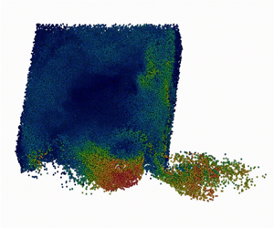
The evolution of transport for Eulerian and Lagrangian cases is depicted in figure 8, showing how the shear-layer vortices emerging at the interface entrap the contaminant in the lateral cavity, transporting mass downstream in the main channel. The time sequence of concentration contours in the Eulerian case, and particles coloured by their velocity magnitude in the Lagrangian simulations, can help visualize the leading role of these large-scale vortices, which also entrain fluid from the main channel into the recirculating region as the cavity is emptied.

Figure 8.

Plan view of transport evolution from the lateral cavity in the Lagrangian (a–c) and Eulerian (d–f) simulations. The sequences show the influence of the shear layer on the mass exchange toward the main channel. Both sequences correspond to one shear-layer period (1.72 s, or 4 non-dimensional times), but they are displayed at different physical times to enhance clarity of the transport processes in each case. Additional details can be observed in the supplementary movies of the paper.

To provide quantitative insights into the global decrease of the concentration in the cavity we study the flux across the interface, which is the large-scale response of the system to the overall effects of the turbulent coherent structures on mass transport, between the channel and the lateral storage zone. For the Lagrangian data we computed the flux as the difference in the number of particles inside the cavity at two consecutive times divided by the total number of particles and the time window. For the Eulerian data we considered the difference in the volume-averaged concentration divided by the time. The time series of mass flux in figure 9, show that the LES captures the periodicity and transport fluctuations across the interface driven by the shear layer. The filtered data at larger time scales show that the leading frequency of transport observed in these plots coincides with the periodic velocities induced by the the vortex shedding at the interface. The fluxes at the interface also show negative excursions, or negative transport, due to the re-entrance of mass in the cavity, which is a phenomenon clearly captured by the Lagrangian model with particle trajectories that perform a complex zigzagging at the interface, as will be subsequently shown (see also Engelen et al. Reference Engelen, Perrot-Minot, Mignot, Rivière and De Mulder2021).

Figure 9.

Time series of Lagrangian and Eulerian mass flux across the cavity interface. The mass exchange reveals a periodicity linked to the vortex-shedding frequency. The figure at the right shows the more fluctuating Lagrangian flux with larger excursions.

To evaluate the mass transport at a global scale, lateral recirculating regions are typically analysed by using transient storage models. A 1-D transport equation for the averaged concentration represents the exchange with the main channel as proportional to the concentration gradient. Through the instantaneous information provided by LES, we can understand in detail the driving mechanisms for the mass exchange and improve the large-scale formulations computing the instantaneous volume-averaged concentration inside the cavity. The global large-scale model represents the time evolution of the concentration in the cavity as follows:

(4.1)\begin{equation} \frac{{\rm d}\langle C\rangle}{{\rm d} t} = \frac{Q_{mc}}{\forall_c} (C_m - \langle C\rangle), \end{equation}

where $\langle C\rangle$ and $C_m$ are the spatially averaged bulk concentration in the cavity and in the main channel respectively, $Q_{mc}$ is the volumetric flux from the main channel to the cavity and $\forall _c$ is the cavity volume. The instantaneous flux across the interface is computed from an exchange velocity across the interface $E$, and is expressed in terms of the interface width $W$

(4.2)\begin{equation} \frac{{\rm d} \langle C\rangle}{{\rm d} t} = \frac{E}{W} (C_m - \langle C\rangle). \end{equation}

The exchange velocity is estimated as proportional to the bulk velocity in the main channel $E=kU_b$, where $k$ is known as the dimensionless mass exchange coefficient. The model for the cavity concentration is written as

(4.3)\begin{equation} \frac{{\rm d} \langle C\rangle}{{\rm d} t} = \frac{k U_b}{W} (C_m - \langle C\rangle). \end{equation}

For the cavity that is initially full, the analytical solution of this equation shows that the concentration decays exponentially, such that

(4.4)\begin{equation} \langle C\rangle/C_0 = e^{{-}t/\tau}, \end{equation}

where $C_0$ is the initial concentration inside the cavity and corresponds to the maximum value, and $\tau$ is the mean residence time, related to the mass exchange coefficient $k$ as follows:

(4.5)\begin{equation} \tau = \frac{W}{k U_b}. \end{equation}

The magnitude of the exchange is typically estimated from experiments, using dye releases or measuring the transverse velocity at the interface, fitting the solution to the data (Knapp & Kelleher Reference Knapp and Kelleher2020). In our numerical simulations we can directly compute the contaminant mass remaining in the cavity, either from the instantaneous concentration field or from the particles in the Lagrangian model.

Figure 10 shows (4.4) with the flux computed from LES in a semilog plot, where the exchange coefficients and time scales associated with this model are related to the slope of the curves. As expected, the Eulerian and Lagrangian results yield different exchange coefficients, due to the mixing effects of the continuum approach. The contaminant is diluted in fluid from the main channel that has been entrained in the cavity by the shear layer. Clear fluid from upstream enters the cavity, facilitating the mixing with the contaminant by advective and diffusive processes. In the Lagrangian model, however, there is no molecular or turbulent mixing. This effect was verified in our calculation by changing the number of particles and by performing an additional Eulerian calculation at a higher temporal resolution, to discard the potential influence of the numerical discretization of the advective terms.

Figure 10.

Comparison for the evolution of averaged concentration from LES, and the large-scale model with a fractional derivative of order $\alpha =0.96$. For Eulerian and Lagrangian cases the global model captures the evolution of the instantaneous mass inside the cavity, representing the memory effects induced by the collective interactions of turbulent coherent structures.

The numerical results show that the exponential decay of this first-order model separates from the actual decay when there is still $40\,\%$ of the initial total mass in the cavity. The exchange coefficient $k$ is estimated from the instantaneous average concentration in the Eulerian case, whereas, for the Lagrangian data, the value of $k$ is obtained by counting the fraction of the initial number of particles that remains inside the cavity over time.

The non-dimensional global residence times obtained from Lagrangian and Eulerian data are $\tau _L=102$ and $\tau _E=130$, respectively. This statistic represents the average time that particles or the passive scalar remain inside the cavity, if we assume that transport is proportional to the concentration difference between the two zones. The mean residence times obtained here are similar to the values obtained by previous studies for cavity flows at different aspect ratios $L/W$ (Jackson et al. Reference Jackson, Haggerty, Apte, Coleman and Drost2012; Sanjou & Nezu Reference Sanjou and Nezu2013; Drost et al. Reference Drost, Apte, Haggerty and Jackson2014). The mass exchange coefficients from Lagrangian and Eulerian data are $k_L=0.042$ and $k_E=0.033$, respectively, and are also consistent with data in the literature for lateral cavity flows (Weitbrecht & Jirka Reference Weitbrecht and Jirka2001; Sanjou & Nezu Reference Sanjou and Nezu2013; Mignot et al. Reference Mignot, Cai, Launay, Riviere and Escauriaza2016, Reference Mignot, Cai, Polanco, Escauriaza and Riviere2017; Sandoval et al. Reference Sandoval, Mignot, Mao, Pastén, Bolster and Escauriaza2019).

From the work of Sandoval et al. (Reference Sandoval, Mignot, Mao, Pastén, Bolster and Escauriaza2019) on a natural lateral cavity, the global model based on a time-fractional differential equation can be used to better describe the evolution of mean concentration in the cavity, which captures the complex emergent dynamics that is the consequence of the interactions of turbulent coherent structures inside the recirculating region. We maintain the same exchange coefficients $k_L=0.042$ and $k_E=0.033$, solving the following equation:

(4.6)\begin{equation} \frac{{\rm d}^\alpha}{{\rm d}t^\alpha}\langle C\rangle={-}\frac{kU_b}{W}\frac{h_m}{h}\left(\langle C\rangle-C_m\right), \end{equation}

where $\alpha$ corresponds to the order of the fractional derivative. The solution of this equation corresponds to a Mittag–Leffler function, which generalizes the exponential solution.

In figure 10 we show that, at short time scales, the first-order linear model represents correctly the initial emptying process that transitions to a heavy-tail behaviour with an apparent change of the decay rate at approximately $t=120$ for $(C=0.4)$. The order of the fractional derivative $\alpha =0.96$ reflects the memory effects induced by the collective dynamics of the turbulent flow. Stronger memory effects have been also observed in natural surface storage zones, enhanced by complex bathymetries that induce upwelling events and large 3-D flow features as discussed in Sandoval et al. (Reference Sandoval, Mignot, Mao, Pastén, Bolster and Escauriaza2019).

All these characteristics observed in the global dynamics of mass transport, such as the periodicity of the fluxes and the evolution of the cavity concentrations that departs from classical gradient diffusion transport, point to the conclusion that multiple time scales influence the exchange with the main channel.

Therefore, memory effects generate a wider distribution of residence times in the cavity. We investigate their distribution by constructing their histogram, as shown in figure 11. The power-law probability density function associated with the memory effects revealed by the fractional model, with the tails decaying with a $-1.96$ slope in a semilog plot, is linked to the exponent of the fractional derivative and represents better the extreme values of the residence time distributions.

Figure 11.

Histogram of Lagrangian residence times in the entire cavity volume, showing the theoretical decay given by the exponential function and the equivalent power-law distribution from the fractional model, which can represent better the extreme values of the distribution.

From the LES results and particle trajectories, we can further analyse the effects of coherent structures on global statistics and identify the topology of the flow in the cavity that explains the global observations in experiments and simulations. In the following sections we study in detail the spatial distribution of the residence times inside the lateral recirculating region, and compute statistics that are closely linked to particle trajectories across the interface.

5. Spatial residence time statistics

The analysis of the global transport reveals a wide distribution of residence times imposed by the turbulent coherent structures of the flow. Three-dimensional maps of the residence time distribution inside the cavity are generated by the following procedure: (a) particles are randomly distributed occupying the entire cavity volume; (b) the Lagrangian simulation is performed, tracking each individual particle position and recording the time they remain inside the cavity (residence time); and (c) after the simulation is finished, the particle initial position is coloured by the residence time obtained in the previous step. Therefore, by analysing how long particles remain inside the cavity and relating it to their initial positions, we can visualize the spatial distribution of these time scales and identify sections with similar residence times occupying distinct volumes inside the cavity.

In figure 12(a) we plot three different planes of the 3-D map of residence times, coloured by their magnitude at the initial location of each particle. The horizontal plane $x\unicode{x2013}y$, and vertical $y\unicode{x2013}z$ and $x\unicode{x2013}z$ planes are organized from top to bottom, showing the large disparity of time scales in the lateral recirculating region, which seem to be organized according to the large-scale vortices observed in the simulations. Two relevant aspects of the Lagrangian mass transport can be visualized: (i) there are global patterns of residence times that appear in the cavity volume, with smaller values near the interface and upstream wall, and a region occupied by longer time scales in the vicinity of the central vortex core; and (ii) inside these global sections that gather trajectories with similar residence times, there is an irregular distribution of scales and local fluctuations induced by turbulence, which are embedded in most of the cavity volume. The blue regions emerge as the clear imprint of shear-layer vortices, with short residence times at the locations close to the interface and return leg of the central core rotation, where these vortices can easily extract a large number of particles from the cavity.

Figure 12.

Spatial distribution of particle residence times according to their initial positions. Slices correspond to $x\unicode{x2013}y$, $y\unicode{x2013}z$ and $x\unicode{x2013}z$ planes from top to bottom. (a) Non-averaged values of initial position of particles coloured by their residence time, showing regions with groups of particles with similar time scales. (b) Values averaged over the first four dimensionless times (equivalent to one shear-layer period).

To reduce the grainy structure produced by local fluctuations, we perform a period-average filtering, based on the scale of the shear layer $T=4.0$, where these specific global regions can be better identified. The plots in figure 12(b) show the same planes but computed with the period-averaged residence time, capturing a clearer spatial distribution of the large-scale global patterns. Regions of different time scales separated by two orders of magnitude are observed, the largest is associated with the main vortex core in the central region, with residence times above 120; and the second at the interface and upstream boundary influenced by the shear layer, with residence times lower than 40. All other regions have residence times between these two values (40–120). This finding is similar to the multiple-region models proposed by Drost et al. (Reference Drost, Apte, Haggerty and Jackson2014) and Sandoval et al. (Reference Sandoval, Mignot, Mao, Pastén, Bolster and Escauriaza2019), which consist of two exchanges zones corresponding to the perimeter of the main eddy and the core of the recirculation region. Our findings, however, differ slightly from those of Drost et al. (Reference Drost, Apte, Haggerty and Jackson2014) and correspond to two regions with completely different time scales: the vortex core time scale ($t_{vc}=150$) and the interface and upstream boundary influenced by the shear-layer time scale ($t_{sl}=4$). We found that all other areas inside the cavity are influenced by more than one time scale and mainly by the eddy turnover time scale ($t_{ed}=50$). Our findings provide a more complete understanding on the identification of regions that trap and release mass in lateral recirculating regions and are in agreement with Juez et al. (Reference Juez, Bühlmann, Maechler, Schleiss and Franca2018a), who observed that sediment particles tended to flow into the core of the main recirculating eddy and settle there (as also discussed in Ouro et al. Reference Ouro, Juez and Franca2020).

The fluctuations and spatial variability observed inside the cavity, as depicted in the fine-grained figure 12(a), indicate that particles starting very close to each other can have significantly different residence times, highlighting the complex Lagrangian dynamics of the flow driven by the interplay between the central slow vortex core motion, and particles approaching the interface that can rapidly leave the cavity or remain inside for arbitrarily long times. A closer analysis of the particle trajectories shows that streamwise vortices between pairs of the columnar vortices that are part of the shear layer induce a vertical motion that reintroduces particles inside the lateral cavity. The sequence of images in figure 13 shows the instantaneous positions coloured by residence time and vertical velocity, in which particles at the interface that approach the region between two vertical axis vortices are re-entrained and remain inside for a longer period. This can be identified by particle pockets of green and yellow residence times at the shear layer. Animations of the flow show that these particles oscillate at the interface, which was described as particle zigzagging by Engelen et al. (Reference Engelen, Perrot-Minot, Mignot, Rivière and De Mulder2021), leaving and re-entering the cavity one or more times. Re-entrained particles by vertical velocity events of longitudinal vortices circle around the central vortex at least once more, adding to their residence time a turnover time scale on average every cycle they remain inside. The vortex dynamics inside the cavity influences the approach trajectory of particles approaching the interface. When they reach the dark blue zones in figure 12, they will likely exit the cavity immediately.

Figure 13.

Sequence of Lagrangian transport across the interface, with particles coloured by residence time (a–c) and vertical velocity (d–f). The re-entrainment of particles at the interface can be identified by particle pockets that sit between two vortices of the shear layer, which are advected back in the cavity by vertical motions. This 3-D effect of streamwise vortices is the leading re-entrainment mechanism.

To summarize the variability of particle residence times we compute the spatial distribution of the standard deviation of local residence time at each point (in units of time) and the non-dimensional coefficient of variation, corresponding to the ratio between the standard deviation and the mean residence time. Since these statistics exhibit a less pronounced variability in horizontal planes, in figure 14 we show depth-averaged magnitudes. The spatial distribution observed in the standard deviation of residence times is influenced by the complex instantaneous dynamics of the shear layer, and connects to the physical mechanisms observed in figure 13. Large and small values of standard deviation are related to regions of small and large residence times, respectively. The red region of large standard deviation at the left in figure 14 coincides with an internal shear layer produced by the vortex core in the centre of the cavity and the return flow near the upstream wall, which divides particles that exit or remain inside, where the latter circle the large-scale vortex one or more times. The coefficient of variation distribution shows the influence of the region between vortices, where there is a large disparity of residence times with respect to the average due to the periodic re-entrainment. Due to the small residence times in these zones, the large coefficient of variation implies that particles reaching these positions oscillate at the interface one or more times to finally exit or remain inside the cavity, and the largest values are explained by this zigzagging at the interface. Particles starting in these regions have residence times lower than 30 or 40, which is less than the time it takes to a particle that start close to the interface and circling the cavity before reaching the interface again.

Figure 14.

Depth-integrated statistics of the residence times in the cavity volume. (a) Standard deviation; and (b) coefficient of variation.

6. Finite-time Lyapunov exponents

The spatial distribution of residence times generated by the coherent structures reveals regions built by particles trajectories that organize the flow into ordered patterns, accumulating trajectories with similar time scales. To formalize the detection of these volumes inside the cavity and at the interface, we study the range of time scales that emerge from the Lagrangian transport, calculating the 3-D finite-time Lyapunov exponents (FTLE) of particle trajectories (Haller Reference Haller2015).

The FTLE are used to measure the rate of separation of neighbouring trajectories over a specific time interval. They are commonly used to identify Lagrangian coherent structures in the flow and to provide a quantitative evaluation of the time scales embedded in the particle transport, which characterize the flow complexity. The technique consists of computing the local flow deformation gradient, through the calculation of the largest stretching of trajectories that begin from a close initial condition, and assumes that the growth of the separation evolves in an exponential fashion, integrated forward in time.

The magnitude of this separation is used to identify flow structures associated with time scales of trajectories. Larger values of FTLE indicate the rate at which nearby particles move apart. We initially consider the uniform spatial distribution of particles inside the cavity at $t=0$, and a varying final integration time $t=T$. The local deformation gradient is a $3\times 3$ matrix at each node of the Eulerian grid based on the derivatives of particle positions. The magnitude of the deformation is the largest eigenvalue $\lambda _{max}$ of the Lagrangian strain tensor $\pmb {\varLambda }$, computed over the time interval

(6.1)\begin{equation} \sigma_{t}^T(x,y,z) = \frac{1}{T} \ln \sqrt{\lambda_{max}(\pmb{\varLambda})}, \end{equation}

where $\sigma _{t}^T(x,y,z)$ is the FTLE at the position $(x,y,z)$ in the time interval $0< t< T$.

In figure 15 we show the 3-D FTLE for a dimensionless time $T=30$, where we can identify three regions inside the cavity. The largest values of FTLE equal to or larger than $\sigma _{t}^{30}=0.17$ can be observed at the interface and in the upstream boundary in blue, whereas the smallest values that are one order of magnitude smaller are encountered at the centre of the cavity in the red region, $\sigma _{t}^{30}=0.08$, which is consistent with the analysis of residence times. The largest values of FTLE in the blue region at the interface and upstream wall, correspond to zones where a significant number of particles leave the cavity and others remain inside, increasing the separation distance. The smallest values of FTLE at the centre of the cavity are due to the longer time scales within the central vortex core, where particles remain for longer periods and their separation evolves slowly. The computation of FTLE for these longer time scales shows that, in the dynamically rich turbulent conditions of the flow, all particle trajectories ultimately diverge from all the regions identified inside the cavity, as they have positive repulsive values of the $\sigma _{t}^{30}$ exponents. The FTLE regions, depicted with different colours in figure 15, provide a simplified skeleton of the overall Lagrangian dynamics inside the cavity that can be used for choosing different zones in multiple-region models that solve a different 1-D mass transport equation for each of these regions (Drost et al. Reference Drost, Apte, Haggerty and Jackson2014; Sandoval et al. Reference Sandoval, Mignot, Mao, Pastén, Bolster and Escauriaza2019).

Figure 15.

Three-dimensional FTLE show regions of the cavity associated with different time scales for an observation period of a non-dimensional time equal to $T=30$.

Similarly, in figure 16 we show horizontal $x\unicode{x2013}y$ planes at middle depth of FTLE for different values of the integral scale $T=1,5,10,30$. In the context of the present simulations, it is important to note that $T=30$ was shown to be better for visualizing the regions of different time scales. Since all particles escape the cavity, the diagrams saturate for larger values of $T$ as particles separate faster when they are transported in the main channel. In figure 16 we show that the largest FTLE values are related to the evolution of the shear layer at the interface from $T=1$ to $T=10$, where the central region between vortices pairs identified in the residence time animation can be distinguished. At $T=30$ not only does the interface have larger values of FTLE but also the upstream boundary of the cavity, which corresponds to the faster-moving region or outer flow that envelops the central core. The FTLE analysis delineates clearly the three regions in the cavity: the shear layer, the intermediate zone of rotating particles and the core with an exponent one order of magnitude smaller. In this last region, around ${35}\,\%$ of the total particles remain when the global concentration is $C=0.4$, occupying the central ${25}\,\%$ of the cavity volume, underscoring its effects on the suppression of global transport for long times.

Figure 16.

Horizontal $x\unicode{x2013}y$ planes of repulsive FTLE at different final times $T=1,5,10,30$ at middle depth $z/h=0.5$; (a) $T=1$, (b) $T=5$, (c) $T=10$, (d) $T=30$.