2. Reduced first-order chains

Let $m \ge 3$. Suppose that $X=\{X_t : t=1, 2, \ldots\}$ is an $(m-1)$th order chain on state space $S=\{1, 2, \ldots, n\}$ whose transition tensor is ${\cal P}=[p_{i_1i_2\ldots i_m}]$. It is well known [Reference Doob5, Reference Hunter16] that this higher-order chain $X$ can be associated with a first-order chain as follows.

First, define the set $T$ of multi-indices of length $m-1$, ordered by linear indexing [Reference Martin, Shafer and Larue26], as

\begin{equation*}T=\{i_1i_2\ldots i_{m-1} : i_1, i_2, \ldots, i_{m-1} \in S\}.\end{equation*}

Note that the cardinality of $T$ is $N=n^{m-1}$. Next, for $t \ge m-1$, introduce vector-valued random variables

\begin{equation*}Y_t=[X_t \ \ X_{t-1} \ \ \ldots \ \ X_{t-m+2}]^T.\end{equation*}

Let us denote $Y_t=i_1i_2\ldots i_{m-1}$ when $X_t=i_1, X_{t-1}=i_2, \ldots, X_{t-m+2}=i_{m-1}$. Then, the vector-valued stochastic process $Y=\{Y_t : t=m-1, m, \ldots\}$ is a first-order chain on state space $T$, which we shall refer to as the reduced first-order chain obtained from $X$.

Denote the $N \times N$ transition matrix of $Y$ by $Q$. It is more convenient to write

\begin{equation*}Q=[q_{i_1i_2\ldots i_{m-1},j_2j_3\ldots j_m}]\end{equation*}

in multi-index form with $i_1i_2\ldots i_{m-1}, j_2j_3\ldots j_m \in T$. Then, the entries of $Q$ can be expressed as, see [Reference Han and Xu12],

\begin{equation*}q_{i_1i_2\ldots i_{m-1}, j_2j_3\ldots j_m}=\left\{\begin{array}{cl} p_{i_1i_2\ldots i_{m-1}j_m}, & ~i_\ell=j_\ell, ~\ell=2, 3, \ldots, m-1;\\ 0, & ~{\rm otherwise.} \end{array}\right.\end{equation*}

In addition, $p_{i_1i_2\ldots i_m}$ is located in $Q$ on row

\begin{equation*}i_1+n(i_2-1)+\ldots +n^{m-2}(i_{m-1}-1)\end{equation*}

and column

\begin{equation*}i_2+n(i_3-1)+\ldots +n^{m-2}(i_m-1).\end{equation*}

For a third-order chain with two states, that is, $m=4$ and $n=2$, for example, we have

\begin{equation*}T=\{111, 211, 121, 221, 112, 212, 122, 222\}\end{equation*}

and

(2.1)\begin{equation} Q=\left[\begin{array}{cccccccc} p_{1111} & 0 & 0 & 0 & p_{1112} & 0 & 0 & 0\\ p_{2111} & 0 & 0 & 0 & p_{2112} & 0 & 0 & 0\\ 0 & p_{1211} & 0 & 0 & 0 & p_{1212} & 0 & 0\\ 0 & p_{2211} & 0 & 0 & 0 & p_{2212} & 0 & 0\\ 0 & 0 & p_{1121} & 0 & 0 & 0 & p_{1122} & 0\\ 0 & 0 & p_{2121} & 0 & 0 & 0 & p_{2122} & 0\\ 0 & 0 & 0 & p_{1221} & 0 & 0 & 0 & p_{1222}\\ 0 & 0 & 0 & p_{2221} & 0 & 0 & 0 & p_{2222} \end{array}\right]. \end{equation}

In particular, $Q$ coincides with the transition matrix of $X$ when this chain is first order, that is, in the special case $m=2$.

Speaking of the connection between a higher-order chain and its reduced first-order chain, we mention here the opinion of Joseph Doob, who has left a profound, lasting impact on the field of stochastic processes. In the seminal monograph [Reference Doob5], he stated that “the generalization (from simple Markov processes to multiple ones) is not very significant, because the (vector) process with random variables $\{\hat{x}_n\}$, ${\hat x}_n=(x_n, \ldots, x_{n+v-1})$ (i.e., $Y_t$ in our notation) has the Markov property ... Thus multiple Markov processes can be reduced to simple ones at the small expense of going to vector-valued random variables.” This appears to suggest that problems regarding a higher-order chain can be solved through its reduced first-order chain.

From what we can gather in literature, different voices have been few and far between. The most notable argument can be found in the classic treatise [Reference Iosifescu17] by Marius Iosifescu, in which he pointed out first that “In this way with any multiple Markov chain one can associate a simple Markov chain. This is the origin of the rooted prejudice that the study of multiple Markov chains reduces to that of simple ones.” and then cited the following example: State $i$ can be recurrent in a second-order chain but $ij \in T$ is not recurrent in the reduced first-order chain for any $j$. This example, albeit useful, falls short to adequately address why it is a “prejudice” to investigate higher-order chains by reducing them to first-order chains, that is, to fully address the key question as raised in the introductory section. Having laid out the notion of reduced first-order chains, we can now rephrase this key questions as:

This formal statement clarifies what the first-order chain is in the previously stated approach “by way of first-order chains.” It is also easier for us to refer to this question in the rest of this article.

3. $k$-step transition and ever-reaching probabilities

Let us begin here with some background material.

For $m, n \ge 2$, let ${\cal A}=[a_{i_1i_2\ldots i_m}]$ and ${\cal B}=[b_{i_1i_2\ldots i_m}]$ be both $m$th order, $n$ dimensional tensors. The tensor product ${\cal A} \boxtimes {\cal B}$ is introduced in [Reference Han and Xu10, Reference Han and Xu12] as an $m$th order, $n$ dimensional tensor ${\cal C}=[c_{i_1i_2\ldots i_m}]$ such that

\begin{equation*}c_{i_1i_2\ldots i_m}=\sum_{j=1}^n a_{i_1ji_2\ldots i_{m-1}}b_{ji_2\ldots i_m}\end{equation*}

for any $1 \le i_1, i_2, \ldots, i_m \le n$. When $m=2$, in particular, ${\cal A}\boxtimes {\cal B}$ reduces to a matrix multiplication. Note, however, that the $\boxtimes$ product is in general not associative whenever $m \ge 3$. As a side remark, the product ${\cal A}\boxtimes {\cal B}$ is originally written as ${\cal B} \boxtimes {\cal A}$ in [Reference Han and Xu10]. The current notation is consistent with the special case when $\cal A$ and $\cal B$ are matrices.

For $k=2, 3, \ldots$, the $k$th power of the $m$th order, $n$ dimensional tensor $\cal A$ is defined recursively by

\begin{equation*}{\cal A}^{k+1}={\cal A}^k \boxtimes {\cal A}, ~k=1, 2, \ldots,\end{equation*}

with ${\cal A}^1=\cal A$. By convention, ${\cal A}^0={\cal I}=[\delta_{i_1i_2\ldots i_m}]$, the $m$th order, $n$ dimensional identity tensor whose entries satisfy

\begin{equation*}\delta_{i_1i_2\ldots i_m}=\left\{\begin{array}{cl} 1, & i_1=i_2;\\ 0, & {\rm otherwise.} \end{array}\right.\end{equation*}

It is easy to see that ${\cal I}\boxtimes {\cal A}=\cal A$, but in general ${\cal A}\boxtimes {\cal I} \ne \cal A$.

Besides the above, the mode- $k$ matricization of the $m$th order, $n$ dimensional tensor $\cal A$ is defined to be an $n$ by $N$, with $N=n^{m-1}$, matrix that has the mode- $k$ fibers ${\cal A}(i_1, \ldots, i_{k-1}, :, i_{k+1}, \ldots, i_m)$ as columns. These fibers are arranged in the linear indexing order of $i_1\ldots i_{k-1}i_{k+1}\ldots i_m$ [Reference Kolda and Bader20]. Especially, the mode- $1$ matricization of $\cal A$ is formed by arranging ${\cal A}(:,:,i_3, \ldots, i_m)$, that is, the frontal slices of $\cal A$, side by side via the linear indexing order of $i_3\ldots i_m$.

As shown in [Reference Han, Wang and Xu9, Reference Han and Xu10, Reference Han and Xu12], the $\boxtimes$ product plays a crucial role in the study of higher-order chains. It can be used to formulate various important quantities such as $k$-step transition probabilities and ever-reaching probabilities, which we shall describe next.

Back to the $(m-1)$th order chain $X$ with state space $S=\{1, 2, \ldots, n\}$ and transition tensor ${\cal P}=[p_{i_1i_2\ldots i_m}]$. Denote ${\cal P}^k=[p^{(k)}_{i_1i_2\ldots i_m}]$. Then, $p^{(k)}_{i_1i_2\ldots i_m}$ is the $k$-step transition probability from states $(i_2, \ldots, i_m)$ to $i_1$ [Reference Han, Wang and Xu9], that is,

\begin{equation*}p^{(k)}_{i_1i_2\ldots i_m}=\Pr(X_{t+k}=i_1 | X_t=i_2, \ldots, X_{t-m+2}=i_m).\end{equation*}

Accordingly, ${\cal P}^k$ is called the $k$-step transition tensor.

Continuing, let

(3.1)\begin{equation} \eta_{i_1i_2\ldots i_m}=\min\{j \ge 1 : X_{m+j-1}=i_1 | X_{m-1}=i_2, \ldots, X_1=i_m\} \end{equation}

be the random variable of the first passage time from states $(i_2, \ldots, i_m)$ to $i_1$. Denote the probability for this passage to happen at $j=k$ by

\begin{equation*}f^{[k]}_{i_1i_2\ldots i_m}=\Pr(\eta_{i_1i_2\ldots i_m}=k).\end{equation*}

In the special case when $k=1$, $f^{[1]}_{i_1i_2\ldots i_m}=p_{i_1i_2\ldots i_m}$. Denote ${\cal F}^{[k]}=[f^{[k]}_{i_1i_2\ldots i_m}]$, which is called the $k$-step first passage time probability tensor. It is known [Reference Han, Wang and Xu9] that

(3.2)\begin{equation} f^{[k+1]}_{i_1i_2\ldots i_m}=\sum_{j \in S, j \ne i_1}f^{[k]}_{i_1ji_2\ldots i_{m-1}}p_{ji_2\ldots i_m}, ~k=1, 2, \ldots, \end{equation}

To express (3.2) via the $\boxtimes$ product, for any $m$th order, $n$ dimensional tensor ${\cal A}=[a_{i_1i_2\ldots i_m}]$, let us define the diagonal tensor ${\cal A}_d=[a^{(d)}_{i_1i_2\ldots i_m}]$ satisfying

\begin{equation*}a^{(d)}_{i_1i_2\ldots i_m}=\left\{\begin{array}{cl} a_{i_1i_1i_3\ldots i_m}, & i_1=i_2;\\ 0, & {\rm otherwise}. \end{array}\right.\end{equation*}

Clearly, (3.2) can now be written simply as

\begin{equation*}{\cal F}^{[k+1]}=({\cal F}^{[k]}-{\cal F}^{[k]}_d)\boxtimes \cal P.\end{equation*}

The probability of ever reaching $i_1$ from $(i_2, \ldots, i_m)$ is given by

\begin{equation*}f_{i_1i_2\ldots i_m}=\Pr(\eta_{i_1i_2\ldots i_m} \lt \infty)=\sum_{k=1}^\infty f^{[k]}_{i_1i_2\ldots i_m},\end{equation*}

or in tensor form, the ever-reaching probability tensor ${\cal F}=[f_{i_1i_2\ldots i_m}]$ can be expressed as

\begin{equation*}{\cal F}=\sum_{k=1}^\infty {\cal F}^{[k]}.\end{equation*}

These results regarding $k$-step transition probabilities and ever-reaching probabilities remain valid for first-order chains. In the first-order case, they can also be written as $P^k=[p^{(k)}_{ij}]$, the $k$-step transition matrix, and $F=[f_{ij}]$, the ever-reaching probability matrix, respectively [Reference Hunter16, Reference Kemeny and Snell19].

In passing, we also give one example of the mode- $1$ matricization of the transition tensor $\cal P$, denoted by $P$. Take a third-order chain with two states just as the one in the previous section, that is, $m=4$ and $n=2$. Then,

\begin{equation*}P=\left[\begin{array}{cc|cc|cc|cc} p_{1111} & p_{1211} & p_{1121} & p_{1221} & p_{1112} & p_{1212} & p_{1122} & p_{1222}\\ p_{2111} & p_{2211} & p_{2121} & p_{2221} & p_{2112} & p_{2212} & p_{2122} & p_{2222} \end{array}\right].\end{equation*}

Clearly, $P$ coincides with the transition matrix when the chain is first order. For $k=0, 1, \ldots$, the mode- $1$ matricization of ${\cal P}^k$ is formed in a similar way and denoted by $P^{(k)}$.

In view of Question 2.1, we now raise the question of whether the $k$-step transition tensor or ever-reaching probability tensor of a higher-order chain can be obtained from their respective counterpart of the reduced first-order chain. Given an $(m-1)$th order, $m \ge 3$, chain with transition tensor $\cal P$, it is shown in [Reference Han and Xu12] that

(3.3)\begin{equation} P^{(k)}=P^{(0)}Q^k, ~k=1, 2, \ldots, \end{equation}

where $P^{(k)}$ and $P^{(0)}$ stand for the mode- $1$ matricizations of ${\cal P}^k$ and ${\cal P}^0={\cal I}$, respectively, and $Q^k$ denotes the $k$-step transition matrix of the associated reduced first-order chain. The formula (3.3) provides a connection between the $k$-step transition probabilities of the higher-order chain and those of its reduced first-order chain. It is worth noting, nevertheless, that these $k$-step transition probabilities of the higher-order case can be obtained directly via ${\cal P}^k$ without resorting to $Q^k$.

The question concerning ever-reaching probabilities will be considered in the next section after the introduction of the notion of ergodicity.

4. Irreducibility, ergodicity, and regularity

Let us begin with several well-known concepts for first-order chains [Reference Hunter16, Reference Kemeny and Snell19]. Suppose that $P=[p_{ij}]$ is the transition matrix of a first-order chain on state space $S$. Then:

• • The chain is irreducible if for any $\emptyset \ne K \subsetneq S$, there exists $p_{ij} \gt 0$ for some $i \in K$ and some $j \in K^c$. In matrix theory, its transition matrix $P$ is also said to be irreducible. The chain is said to be reducible if it is not irreducible.

• • The chain is ergodic if for any $i, j \in S$, there exists $k \ge 1$, which may depend on $i$ and $j$, such that $p^{(k)}_{ij} \gt 0$.

• • The chain is regular if there exists some $k \ge 1$ such that $p^{(k)}_{ij} \gt 0$ for all $i, j \in S$, that is, $P^k \gt 0$. In matrix theory, such $P$ is said to be primitive.

For a first-order chain, it is well known [Reference Horn and Johnson14] that irreducibility is equivalent to ergodicity.

The above definitions can be extended as follows to a higher-order chain on state space $S$, whose transition tensor is ${\cal P}=[p_{i_1i_2\ldots i_m}]$.

• • The chain is said to be irreducible if for each $\emptyset \ne K \subsetneq S$, there exists $p_{i_1i_2\ldots i_m} \gt 0$ for some $i_1 \in K$ and some $i_2,\ldots,i_m \in K^c$ [Reference Li and Ng24].

• • The chain is said to be ergodic if for any $i_1, i_2, \ldots, i_m \in S$, there exists $k \ge 1$, which may depend on $i_1, i_2, \ldots, i_m$, such that $p^{(k)}_{i_1i_2\ldots i_m} \gt 0$ [Reference Han, Wang and Xu9].

• • The chain is said to be regular if there exists $k \ge 1$ such that for any $i_1, i_2, \ldots, i_m \in S$, $p^{(k)}_{i_1i_2\ldots i_m} \gt 0$, that is, ${\cal P}^k \gt 0$ [Reference Han and Xu12].

Unlike the first-order case, for a higher-order chain, ergodicity is a stronger condition than irreducibility [Reference Han, Wang and Xu9], that is, an ergodic higher-order chain must be irreducible, but the converse is not true in general. Consider, for example, a second-order chain with three states and transition tensor

\begin{equation*}{\cal P}(:,:,1)=\left[\begin{array}{ccc} 0 & 0 & 0\\ 1 & 0 & 0\\ 0 & 1 & 1 \end{array}\right], ~{\cal P}(:,:,2)=\left[\begin{array}{ccc} 0 & 0 & 0\\ 0 & 0 & 0\\ 1 & 1 & 1 \end{array}\right], ~{\cal P}(:,:,3)=\left[\begin{array}{ccc} 0 & 0 & 1\\ 0 & 0 & 0\\ 1 & 1 & 0 \end{array}\right].\end{equation*}

This chain is irreducible, but not ergodic since $p^{(k)}_{2i_2i_3}=0$ for all $1 \le i_2, i_3 \le 3$ and $k \ge 2$.

In order to guarantee the mean first passage times to be well defined and finite, for example, ergodicity is an important condition no matter the order of a chain [Reference Han and Xu10, Reference Kemeny and Snell19]. Following Question 2.1, it is natural to ask whether the mean first passage times of a higher-order chain can be obtained from those of its reduced first-order chain. First and foremost, however, it makes sense to ask whether ergodicity of a higher-order chain carries over to its reduced first-order chain. The answer to the latter question, unfortunately, turns out to be negative as shown by the following example.

Let ${\cal P}=[p_{i_1i_2i_3}]$ be the transition tensor of a second-order chain of three states such that all $p_{i_1i_2i_3}$ are positive except $p_{311}=p_{312}=p_{313}=0$. Let us simply take

\begin{equation*}{\cal P}(:,:,1)={\cal P}(:,:,2)={\cal P}(:,:,3)=\left[\begin{array}{ccc} 1/2 & 1/3 & 1/3\\ 1/2 & 1/3 & 1/3\\ 0 & 1/3 & 1/3 \end{array}\right].\end{equation*}

Since ${\cal P}^2 \gt 0$, this chain is regular and thus is also ergodic. Its reduced first-order chain has transition matrix

\begin{equation*}Q=\left[\begin{array}{ccccccccc} 1/2 & 0 & 0 & 1/2 & 0 & 0 & 1/2 & 0 & 0 \\ 1/2 & 0 & 0 & 1/2 & 0 & 0 & 1/2 & 0 & 0 \\ 0 & 0 & 0 & 0 & 0 & 0 & 0 & 0 & 0 \\ 0 & 1/3 & 0 & 0 & 1/3 & 0 & 0 & 1/3 & 0 \\ 0 & 1/3 & 0 & 0 & 1/3 & 0 & 0 & 1/3 & 0 \\ 0 & 1/3 & 0 & 0 & 1/3 & 0 & 0 & 1/3 & 0 \\ 0 & 0 & 1/3 & 0 & 0 & 1/3 & 0 & 0 & 1/3 \\ 0 & 0 & 1/3 & 0 & 0 & 1/3 & 0 & 0 & 1/3 \\ 0 & 0 & 1/3 & 0 & 0 & 1/3 & 0 & 0 & 1/3 \end{array}\right],\end{equation*}

which is clearly not even irreducible due to its third row of all zeros. Hence, the reduced first-order chain is not ergodic.

The above example also justifies that, like ergodicity, regularity does not carry over either from a higher-order chain to its reduced first-order chain.

What this example demonstrates is, in fact, the first obstacle to studying a higher-order chain through its reduced first-order chain. We shall demonstrate later in Section 6 that other difficulties may arise even if ergodicity or regularity happens to carry over to the reduced first-order chain. The issue of mean first passage times will be addressed there too.

Returning to the question raised in the preceding section concerning the relationship between the ever-reaching probabilities of a higher-order chain and those of its reduced first-order chain, we consider below a second-order chain with four states and transition tensor

\begin{equation*}{\cal P}(:,:,1)=\left[\begin{array}{cccc} 1/2 & 0 & 0 & 0\\ 1/2 & 0 & 1 & 0\\ 0 & 1 & 0 & 1\\ 0 & 0 & 0 & 0 \end{array}\right], ~{\cal P}(:,:,2)=\left[\begin{array}{cccc} 0 & 0 & 1/2 & 1\\ 0 & 1/2 & 0 & 0\\ 1/2 & 1/2 & 0 & 0\\ 1/2 & 0 & 1/2 & 0 \end{array}\right],\end{equation*}

\begin{equation*}{\cal P}(:,:,3)=\left[\begin{array}{cccc} 0 & 1 & 0 & 1\\ 1 & 0 & 1/2 & 0\\ 0 & 0 & 1/2 & 0\\ 0 & 0 & 0 & 0 \end{array}\right], ~{\cal P}(:,:,4)=\left[\begin{array}{cccc} 0 & 0 & 0 & 0\\ 1 & 1 & 1 & 0\\ 0 & 0 & 0 & 1/2\\ 0 & 0 & 0 & 1/2 \end{array}\right].\end{equation*}

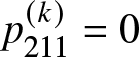
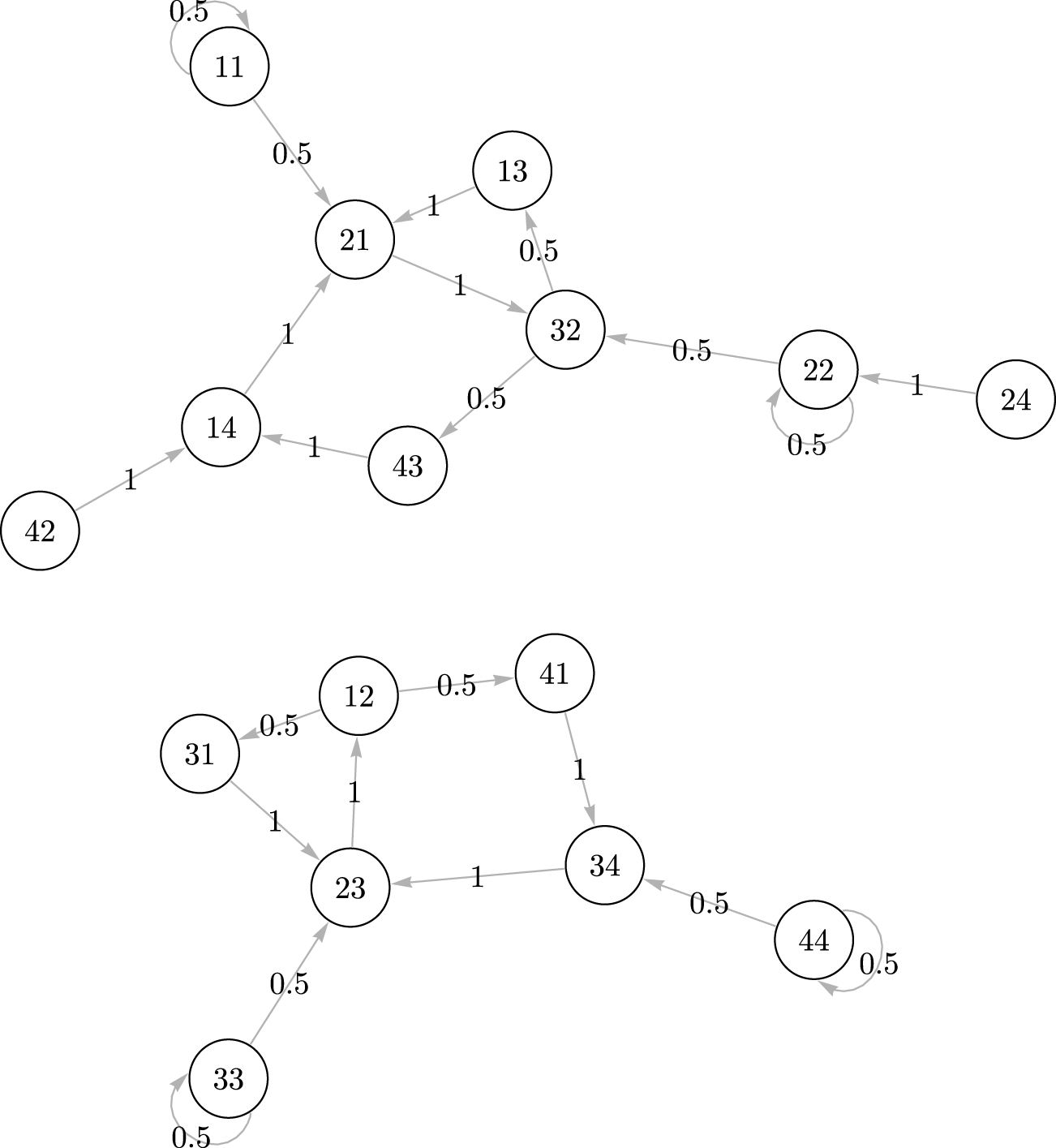
It is easy to verify ${\cal P}^{10} \gt 0$. Clearly, this chain is regular and, consequently, ergodic. It is shown in [Reference Han and Xu10] that for such an ergodic chain, its ever-reaching probabilities $f_{i_1i_2i_3}=1$ for all $1 \le i_1, i_2, i_3 \le 4$. The associated reduced first-order chain, however, exhibits a noticeably different dynamics as illustrated by the digraph in Figure 1 that represents its transition matrix $Q$. Starting, for example, from state $12$, the reduced first-order chain has zero probability of reaching state $11$. This, nevertheless, does not lead to the conclusion that state $1$ cannot be reached from states $(1, 2)$ in the second-order chain since $f_{112}=1$. This illustrates that the answer to Question 2.1 is negative when dealing with the problem of ever-reaching probabilities.

Figure 1. Digraph of reduced first-order chain.

It is quite straightforward, though a bit tedious, to show that the ever-reaching probabilities of a higher-order chain cannot be obtained via those of its reduced first-order chain in a similar manner as neat as (3.3). Again, we consider the general third-order chain with two states in Section 2. Let $G^{[2]}=[g^{[2]}_{i_1i_2i_3, j_1j_2j_3}]$ be the $2$-step first passage time probability matrix of the reduced first-order chain. Then, it is easy to verify that

(4.1)\begin{equation} g^{[2]}_{i_1i_2i_3, j_1j_2j_3}=p_{i_1i_2i_3j_2}p_{i_2i_3j_2j_3}, ~i_1i_2i_3, j_1j_2j_3 \in T, \end{equation}

provided $j_1=i_3$ and either $i_1 \ne i_2$ or $i_2 \ne i_3$ or $i_3 \ne j_2$. As a comparison, it follows from (2.1) that

(4.2)\begin{equation} q^{(2)}_{i_1i_2i_3, i_3j_2j_3}=p_{i_1i_2i_3j_2}p_{i_2i_3j_2j_3}. \end{equation}

Clearly, (4.1) is much more complicated than (4.2). This, together with the preceding example as illustrated in Figure 1, offers an additional perspective showing that the answer to Question 2.1 is negative as far as ever-reaching probabilities are concerned.

5. Classification of states

Given a first-order chain with transition matrix $P=[p_{ij}]$ and ever-reaching probability matrix $F=[f_{ij}]$, it is well known [Reference Hunter16] that:

• • A state $i$ is recurrent if $f_{ii}=1$. A state $i$ is recurrent iff $\displaystyle \sum_{k=1}^\infty p^{(k)}_{ii}=\infty.$

• • A state $i$ is transient if $f_{ii} \lt 1$. A state $i$ is transient iff $\displaystyle \sum_{k=1}^\infty p^{(k)}_{ii} \lt \infty.$

• • A state $i$ is absorbing if $p_{ii}=1$.

The example that is cited by [Reference Iosifescu17], see the introductory section, indicates that the states of a higher-order chain cannot be classified according to the states of its reduced first-order chain. A more complete classification scheme for states of higher-order chains is recently proposed in [Reference Han and Xu11]. Here is a brief description of this scheme. Consider a higher-order chain whose state space is $S$, transition tensor is ${\cal P}=[p_{i_1i_2\ldots i_m}]$, and ever-reaching probability tensor is ${\cal F}=[f_{i_1i_2\ldots i_m}]$. Then,

• • A state $i$ is said to be recurrent if $f_{iii_3\ldots i_m}=1$ for all $i_3, \ldots, i_m \in S$. If state $i$ is recurrent, then $\displaystyle \sum_{k=1}^\infty p^{(k)}_{iii_3\ldots i_m}=\infty$ for all $i_3, \ldots, i_m \in S$.

• • A state $i$ is said to be transient if $f_{iii_3\ldots i_m} \lt 1$ for some $i_3, \ldots, i_m \in S$. Especially, a state $i$ is said to be fully transient if $f_{iii_3\ldots i_m} \lt 1$ for any $i_3, \ldots, i_m \in S$. When state $i$ is fully transient, $\displaystyle \sum_{k=1}^\infty p^{(k)}_{iii_3\ldots i_m} \lt \infty$ for all $i_3, \ldots, i_m \in S$.

• • A state $i$ is said to be absorbing if $p_{iii_3\ldots i_m}=1$ for all $i_3, \ldots, i_m \in S$.

These results from [Reference Han and Xu11] seem to be parallel to their first-order counterparts. We, however, point out some differences between the higher-order and first-order cases. Specifically, for a higher-order chain:

• • There may exist the scenario where a state $i$ is transient but not fully transient, that is, $f_{iii_3\ldots i_m}$ is smaller than $1$ for some $i_3, \ldots, i_m \in S$ but is equal to $1$ for other $i_3, \ldots, i_m \in S$. This is indeed at the center of the key differences between the higher-order and first-order chains when it comes to the classification of states.

• • The condition of whether $\displaystyle \sum_{k=1}^\infty p^{(k)}_{iii_3\ldots i_m}$ is infinite or finite becomes necessary, but not sufficient, for characterizing recurrence or full transience; see the next example.

Before proceeding, we need to introduce a few terms. A state $j$ is said to be reachable from state $i$, denoted as $i \rightarrow j$, if there exists $k \ge 0$, which may depend on $j, i, i_3, \ldots, i_m$, such that $p^{(k)}_{jii_3\ldots i_m} \gt 0$ or, equivalently, $f_{jii_3\ldots i_m} \gt 0$, for all $i_3, \ldots, i_m \in S$. In addition, states $i$ and $j$ are said to communicate, denoted by $i \leftrightarrow j$, if $i \rightarrow j$ and $j \rightarrow i$. The $\leftrightarrow$ relationship is an equivalence relationship and thus it partitions the state space $S$ into equivalence classes [Reference Han and Xu11].

As illustrated in [Reference Han and Xu11], there are quite a few other differences when we go from first-order to higher-order chains regarding the classification of states. For example,

• • A first-order chain must have a recurrent state, but not so for a higher-order chain. Take a second-order chain on three states with transition tensor

  \begin{equation*}{\cal P}(:,:,1)=\left[\begin{array}{ccc} 1 & 0 & 0\\ 0 & 1/2 & 1/2\\ 0 & 1/2 & 1/2 \end{array}\right], ~{\cal P}(:,:,2)=\left[\begin{array}{ccc} 1 & 0 & 1/2\\ 0 & 1 & 0\\ 0 & 0 & 1/2 \end{array}\right], ~{\cal P}(:,:,3)=\left[\begin{array}{ccc} 0 & 1/2 & 1\\ 0 & 1/2 & 0\\ 1 & 0 & 0 \end{array}\right].\end{equation*}

  Then,

  \begin{equation*}{\cal F}(:,:,1)=\left[\begin{array}{ccc} 1 & 1/2 & 3/4\\ 0 & 1 & 1\\ 0 & 1/2 & 1/2 \end{array}\right], ~{\cal F}(:,:,2)=\left[\begin{array}{ccc} 1 & 0 & 1\\ 0 & 1 & 1\\ 0 & 0 & 1 \end{array}\right], ~{\cal F}(:,:,3)=\left[\begin{array}{ccc} 3/4 & 1/2 & 1\\ 1 & 1/2 & 1\\ 1 & 0 & 1 \end{array}\right].\end{equation*}

  For each $1 \le i \le 3$, its ever-reaching probability $f_{iii_3}$ equals $1$ for some $i_3$ and is less than $1$ for some other $i_3$. Consequently, none of the states in this example are recurrent. In addition, we see

  \begin{equation*}\sum_{k=1}^\infty p^{(k)}_{11i_3}=\infty \ \ {\rm and} \ \ \sum_{k=1}^\infty p^{(k)}_{33i_3} \lt \infty\end{equation*}
  for all $1 \le i_3 \le 3$, implying that whether $\displaystyle \sum_{k=1}^\infty p^{(k)}_{iii_3\ldots i_m}$ is infinite or not for all $i_3, \ldots, i_m \in S$ is only a necessary condition for recurrence or full transience, respectively.

• • In a first-order chain, a state $i$ is recurrent provided $j \rightarrow i$ whenever $i \rightarrow j$. Such a characterization does not apply to a higher-order chain. Consider a second-order chain with two states and transition tensor

  \begin{equation*}{\cal P}(:,:,1)=\left[\begin{array}{cc} 1 & 1/2\\ 0 & 1/2 \end{array}\right], ~{\cal P}(:,:,2)=\left[\begin{array}{cc} 0 & 1/2\\ 1 & 1/2 \end{array}\right].\end{equation*}

  It follows

  \begin{equation*}{\cal F}(:,:,1)=\left[\begin{array}{cc} 1 & 1\\ 0 & 1 \end{array}\right], ~{\cal F}(:,:,2)=\left[\begin{array}{cc} 1 & 1\\ 1 & 1 \end{array}\right].\end{equation*}

  Both states are recurrent since $f_{iii_3}=1$ for all $i, i_3=1, 2$. Meanwhile, $2 \rightarrow 1$ yet $1 \not\rightarrow 2$ since $p^{(k)}_{i_1i_2i_3} \gt 0$ for all $1 \le i_1, i_2 \le 2$ and $k \ge 2$ but $p^{(k)}_{211}=0$ for all $k \ge 1$.

• • In a first-order chain, both recurrence and transience are class properties, that is, the states in an equivalence class must be either all recurrent or all transient. When it comes to a higher-order chain, recurrence and transience are not class properties anymore. To see this, we examine a second-order chain with three states and transition tensor

  \begin{equation*}{\cal P}(:,:,1)=\left[\begin{array}{ccc} 1/2 & 1/3 & 1/2\\ 1/2 & 1/2 & 0\\ 0 & 1/3 & 1/2 \end{array}\right], ~{\cal P}(:,:,2)=\left[\begin{array}{ccc} 1 & 0 & 1/2\\ 0 & 1 & 1/2\\ 0 & 0 & 0 \end{array}\right], ~{\cal P}(:,:,3)=\left[\begin{array}{ccc} 0 & 0 & 1/2\\ 0 & 0 & 1/2\\ 1 & 1 & 0 \end{array}\right].\end{equation*}

  For this chain, we have

  \begin{equation*}{\cal F}(:,:,1)=\left[\begin{array}{ccc} 5/6 & 2/3 & 1\\ 1 & 1 & 1\\ 1/2 & 1/2 & 1 \end{array}\right], ~{\cal F}(:,:,2)=\left[\begin{array}{ccc} 1 & 0 & 1\\ 1 & 1 & 1\\ 1/2 & 0 & 1 \end{array}\right], ~{\cal F}(:,:,3)=\left[\begin{array}{ccc} 1 & 1 & 1\\ 1 & 1 & 1\\ 1 & 1 & 1 \end{array}\right].\end{equation*}

  By checking its ever-reaching probabilities $f_{iii_3}$, state $1$ is transient but not fully transient, and state $3$ is recurrent. These states, however, are in the same equivalence class, that is, $1 \leftrightarrow 3$.

Such differences constitute yet another roadblock to studying a higher-order chain via its reduced first-order chain. Thus, as far as classification of states is concerned, the answer to Question 2.1 is again negative.

The following was conjectured in [Reference Han and Xu11]. To end this section, we shall prove it here.

Proof. Let $i, j \in K$, $i \ne j$, with $j$ being recurrent. Then, it suffices to show that $i$ cannot be fully transient.

Let us fix $i_3, \ldots, i_m$. Since $i \rightarrow j$ and $i \ne j$, there exists $\alpha \ge 1$ such that $p^{(\alpha)}_{jii_3\ldots i_m} \gt 0$. Denote the event “the chain takes $\alpha$ steps to go from $ii_3\ldots i_m$ to $j$” by $A$.

Next, denote the event “starting from $jj_3\ldots j_m$, the chain takes $\beta$ steps to return to $j$” by $B$, where $j_3, \ldots, j_m$ are given by:

• • when $\alpha=1$: $j_3=i, j_4=i_3, \ldots, j_m=i_{m-1}$

• • when $\alpha=2$: $j_4=i, j_5=i_3, \ldots, j_m=i_{m-2}$, any $j_3$

• • $\cdots$

• • when $\alpha=m-2$: $j_m=i$, any $j_3,\ldots,j_{m-1}$

• • $\cdots$

Fix $j_3, \ldots, j_m$ from now on.

Next, denote the event “the chain takes $\gamma$ steps to go from $jk_3\ldots k_m$ to $i$” by $C$, where $k_3, \ldots, k_m$ are determined in the same way as $j_3, \ldots, j_m$ above.

From this point on, let us assume $\beta \ge m-1$. Thus, we can fix $k_3, \ldots, k_m$. Accordingly, by $j \rightarrow i$ and $i \ne j$, there exists $\gamma \ge 1$ such that $p^{(\gamma)}_{ijk_3\ldots k_m} \gt 0$.

Finally, we observe

\begin{align*} p^{(\gamma+\beta+\alpha)}_{iii_3\ldots i_m} & \ge \Pr(ABC)\\ & = \Pr(A)\Pr(B|A)\Pr(C|AB)\\ & = p^{(\alpha)}_{jii_3\ldots i_m}p^{(\beta)}_{jjj_3\ldots j_m}p^{(\gamma)}_{ijk_3\ldots k_m}. \end{align*}

It follows that

\begin{equation*}\sum_{\beta=m-1}^\infty p^{(\gamma+\beta+\alpha)}_{iii_3\ldots i_m} \ge p^{(\alpha)}_{jii_3\ldots i_m}p^{(\gamma)}_{ijk_3\ldots k_m}\sum_{\beta=m-1}^\infty p^{(\beta)}_{jjj_3\ldots j_m}=\infty\end{equation*}

since $j$ is recurrent. The above clearly leads to

\begin{equation*}\sum_{\beta=1}^\infty p^{(\beta)}_{iii_3\ldots i_m}=\infty.\end{equation*}

The proof is now complete.

6. Mean first passage times

For convenience, let us use a framework that includes both higher-order and first-order chains.

Recall $\eta_{i_1i_2\ldots i_m}$ in (3.1). For an $(m-1)$th order, $m \ge 2$, chain with state space $S=\{1, 2, \ldots, n\}$, the mean first passage time from states $(i_2, \ldots, i_m)$ to $i_1$ is defined by

\begin{equation*}\mu_{i_1i_2\ldots i_m}={\rm E}(\eta_{i_1i_2\ldots i_m})=\sum_{k=1}^\infty k\Pr(\eta_{i_1i_2\ldots i_m}=k).\end{equation*}

Accordingly, the mean first passage time tensor is the $m$th order, $n$ dimensional tensor $\mu=[\mu_{i_1i_2\ldots i_m}]$.

As shown in [Reference Han and Xu10], for an ergodic higher-order chain of order $m-1$ whose $m$th order, $n$ dimensional transition tensor is $\cal P$, its mean first passage times are finite and are uniquely determined by the following tensor equation:

(6.1)\begin{equation} \mu={\cal E}+(\mu-\mu_d)\boxtimes {\cal P}, \end{equation}

where $\cal E$ is the $m$th order, $n$ dimensional tensor of all ones. Furthermore, as a linear system, (6.1) is nonsingular if and only if the chain is ergodic.

Comparing with an ergodic first-order chain, the mean first passage time matrix $M$ satisfies [Reference Kemeny and Snell19]

(6.2)\begin{equation} M=E+(M-M_d)P, \end{equation}

where $E$ is the matrix of all ones and $M_d=[m^{(d)}_{ij}]$ is such that

\begin{equation*}m^{(d)}_{ij}=\left\{\begin{array}{cl} m_{ii}, & i=j;\\ 0, & {\rm otherwise}. \end{array}\right.\end{equation*}

Clearly, (6.2) is a special case of (6.1). Because of the resemblance between (6.1) and (6.2), and in the spirit of Question 2.1, it is an intriguing question whether (6.1) can be derived from (6.2) using the reduced first-order chain. The answer, however, turns out to be negative, as illustrated by the example below.

Take a second-order chain with three states and

\begin{equation*}{\cal P}(:,:,1)={\cal P}(:,:,2)={\cal P}(:,:,3)=\left[\begin{array}{ccc} 1/3 & 1/3 & 1/3\\ 1/3 & 1/3 & 1/3\\ 1/3 & 1/3 & 1/3 \end{array}\right].\end{equation*}

By solving (6.1),

\begin{equation*}\mu(:,:,1)=\mu(:,:,2)=\mu(:,:,3)=\left[\begin{array}{ccc} 3 & 3 & 3\\ 3 & 3 & 3\\ 3 & 3 & 3 \end{array}\right].\end{equation*}

On the other hand, observing that the regularity of this second-order chain carries over to its reduced first-order chain since $Q^2=(1/9)E \gt 0$, where $E$ is the matrix of all ones, and using (6.2) for the reduced first-order chain, we obtain

\begin{equation*}M=\left[\begin{array}{ccccccccc} 9 & 12 & 12 & 9 & 12 & 12 & 9 & 12 & 12\\ 6 & 9 & 9 & 6 & 9 & 9 & 6 & 9 & 9\\ 6 & 9 & 9 & 6 & 9 & 9 & 6 & 9 & 9\\ 9 & 6 & 9 & 9 & 6 & 9 & 9 & 6 & 9\\ 12 & 9 & 12 & 12 & 9 & 12 & 12 & 9 & 12\\ 9 & 6 & 9 & 9 & 6 & 9 & 9 & 6 & 9\\ 9 & 9 & 6 & 9 & 9 & 6 & 9 & 9 & 6\\ 9 & 9 & 6 & 9 & 9 & 6 & 9 & 9 & 6\\ 12 & 12 & 9 & 12 & 12 & 9 & 12 & 12 & 9 \end{array}\right].\end{equation*}

Obviously, in this example, $\mu$ does not follow directly from $M$. If we look at $m_{11}$, for instance, it represents the mean first passage time from state $11$, in multi-index form, to itself. This quantity, however, is different from $\mu_{111}$. In other words, while addressing Question 2.1, other difficulties may still arise even if ergodicity or regularity does carry forward from a higher-order chain to its reduced first-order chain.

One way of working around the discrepancy as shown above between the mean first passage times of a higher-order chain and those of its reduced first-order chain is to resort to certain matricization of the transition tensor [Reference Han and Xu10]. This approach is not as convenient as the direct tensor treatment leading to (6.1). Besides, its result can be easily obtained by matricizing the mean first passage time tensor from (6.1).

7. Limiting probability distributions

Having presented a range of differences between higher-order and first-order chains in previous sections, we now come to a point where these two appear to converge to a certain level. Again, we use here a framework that includes both higher-order and first-order chains.

With $m \ge 2$, let $X=\{X_t : t=1, 2, \ldots\}$ be an $(m-1)$th order chain on state space $S=\{1, 2, \ldots, n\}$ whose transition tensor is ${\cal P}=[p_{i_1i_2\ldots i_m}]$. The probability distribution of $X$ at $t$ is given by

\begin{equation*}x_t=[\Pr(X_t=1) ~\Pr(X_t=2) ~\ldots ~\Pr(X_t=n)]^T.\end{equation*}

If there exists an $n$-vector $\pi$, which is independent of the initial probability distributions $x_1, x_2, \ldots, x_{m-1}$, such that

\begin{equation*}\lim_{t \rightarrow \infty}x_t=\pi,\end{equation*}

then $\pi$ is called the limiting probability distribution of the chain $X$[Reference Han and Xu12]. It is clear that $\pi$ satisfies $\pi \ge 0$ and $\displaystyle \sum_{i \in S}\pi_i=1$.

On the other hand, let $Y$ be the reduced first-order chain associated with $X$, whose transition matrix is given by $Q$. Then, an $N$-vector $\xi$ is said to be a stationary distribution of both the chains $X$ and $Y$ if $\xi$ satisfies $\xi \ge 0$, $\displaystyle \sum_{i_1i_2\ldots i_{m-1} \in T}\xi_{i_1i_2\ldots i_{m-1}}=1$, and $Q\xi=\xi$. The subscript for the entries of $\xi$ is written here in multi-index form. Consequently, $Q\xi=\xi$ translates to

\begin{equation*}\sum_{j \in S}p_{i_1i_2\ldots i_{m-1}j}\xi_{i_2\ldots i_{m-1}j}=\xi_{i_1i_2\ldots i_{m-1}}, ~i_1, i_2, \ldots, i_{m-1} \in S,\end{equation*}

which is precisely how a stationary distribution is equivalently defined in [Reference Gleich, Lim and Yu8] when $\xi$ is treated as an $(m-1)$th order, $n$ dimensional tensor. Obviously, as a vector, $\xi$ is just a normalized right eigenvector of $Q$ corresponding to the dominant eigenvalue $\lambda=1$, sometimes also called a Perron vector [Reference Horn and Johnson14].

It is shown in [Reference Han and Xu12] that if the chain $X$ is regular, then its limiting probability distribution $\pi$ is guaranteed to exist. In this case, $\pi \gt 0$ and

\begin{equation*}\lim_{k \rightarrow \infty}{\cal P}^k=\pi \otimes \underbrace{e \otimes \cdots \otimes e}_{m-1},\end{equation*}

where, and in what follows, $e$ is the $n$-vector of all ones and $\otimes$ is the outer product. Without the regularity condition on $X$, $\pi$ may not exist and therefore such a condition is tight.

Regarding a stationary distribution of the chains $X$ and $Y$, its existence is guaranteed following the celebrated Perron–Frobenius theorem, yet such a distribution may not be unique. If, in addition, $Y$ is a regular chain, then its stationary distribution $\xi$ is unique and $\xi \gt 0$.

The preceding results regarding the limiting probability distribution and stationary distribution continue to hold when the chain $X$ is first order and regular [Reference Hunter16, Reference Kemeny and Snell19]. In this scenario, the limiting probability distribution is the same as the stationary distribution. To be more specific, on letting $P$ be the transition matrix, then there exists a unique $n$-vector $\pi \gt 0$ with $\displaystyle \sum_{i \in S}\pi_i=1$ such that $\displaystyle \lim_{k \rightarrow \infty}P^k=\pi e^T$ and, at the same time, $P\pi=\pi$ [Reference Kemeny and Snell19]. This appears to be the cause of why the nomenclatures “limiting probability distribution” and “stationary distribution” are at times used interchangeably in works on higher-order chains. Our foregoing description of these concepts clarifies the difference between them in the higher-order case.

Despite the differences, there is a principal connection between them too. As shown in [Reference Han and Xu12], when the chain $X$ is higher order and regular, its limiting probability distribution $\pi$ can be determined via any stationary distribution $\xi$ through

(7.1)\begin{equation} \pi=P^{(0)}\xi, \end{equation}

where $P^{(0)}$ stands for the mode- $1$ matricization of the $m$th order, $n$ dimensional identity tensor. This result does not require the chain $Y$ to be regular.

To illustrate the usage of (7.1), let us take the same regular second-order chain as in Section 4 with four states and transition tensor

\begin{equation*}{\cal P}(:,:,1)=\left[\begin{array}{cccc} 1/2 & 0 & 0 & 0\\ 1/2 & 0 & 1 & 0\\ 0 & 1 & 0 & 1\\ 0 & 0 & 0 & 0 \end{array}\right], ~{\cal P}(:,:,2)=\left[\begin{array}{cccc} 0 & 0 & 1/2 & 1\\ 0 & 1/2 & 0 & 0\\ 1/2 & 1/2 & 0 & 0\\ 1/2 & 0 & 1/2 & 0 \end{array}\right],\end{equation*}

\begin{equation*}{\cal P}(:,:,3)=\left[\begin{array}{cccc} 0 & 1 & 0 & 1\\ 1 & 0 & 1/2 & 0\\ 0 & 0 & 1/2 & 0\\ 0 & 0 & 0 & 0 \end{array}\right], ~{\cal P}(:,:,4)=\left[\begin{array}{cccc} 0 & 0 & 0 & 0\\ 1 & 1 & 1 & 0\\ 0 & 0 & 0 & 1/2\\ 0 & 0 & 0 & 1/2 \end{array}\right].\end{equation*}

The associated reduced first-order chain is reducible, which can also be seen from the fact that the dominant eigenvalue $\lambda=1$ of its transition matrix $Q$ has multiplicity $2$. This, of course, implies that the reduced first-order chain is not regular. It is easy to verify that

\begin{equation*}\displaystyle z=\frac{1}{7}[0 ~~0 ~~1 ~~1 ~~2 ~~0 ~~0 ~~0 ~~0 ~~2 ~~0 ~~0 ~~0 ~~0 ~~1 ~~0]^T\end{equation*}

is a normalized right eigenvector corresponding to that dominant eigenvalue above. Hence, the limiting probability distribution of the second-order chain is

\begin{equation*}\pi=P^{(0)}z=\frac{1}{7}[2 ~~2 ~~2 ~~1]^T.\end{equation*}

Regarding Question 2.1, when it comes to the limiting probability distribution problem of a higher-order chain, (7.1) represents its close tie with a stationary distribution of the corresponding reduced first-order chain. This, along with the $k$-step transition probabilities in Section 3, is another case in which Question 2.1 yields a positive answer.