





1. Introduction
A distinguishing feature of turbulent flows is its ability to mix efficiently, which plays an important role in combustion systems, mixing of nutrients in the ocean and the dispersion of pollutants, among others. In many of these systems, the species being mixed can bemodelled as passive scalars which do not affect the advecting velocity field. Their dynamics is governed by the advection–diffusion equation with a stirring velocity field that satisfies the Navier–Stokes (NS) equations. The relevant non-dimensional parameter characterising the scalar is the Schmidt number, which is the ratio of momentum to scalar diffusivity ( $Sc\equiv \nu /D$
where
$Sc\equiv \nu /D$
where $\nu$
is the viscosity and
$\nu$
is the viscosity and $D$
the diffusivity coefficient of the scalar), and it can vary from
$D$
the diffusivity coefficient of the scalar), and it can vary from $10^{-6}$
in astrophysical flows (strongly diffusive scalars) to
$10^{-6}$
in astrophysical flows (strongly diffusive scalars) to $10^3$
(weakly diffusive scalars) for laboratory experiments. As the stirring mechanism for scalars is driven by the turbulent velocity field, one would expect that the characteristics of mixing would depend on the properties of the velocity field. Classical phenomenology, however, suggests universal behaviour regardless of the details of the stirring mechanism of both velocity and scalar fields. These opposing viewpoints have been illustrated by Kraichnan (Reference Kraichnan1968) who showed that the scalar spectrum retains the
$10^3$
(weakly diffusive scalars) for laboratory experiments. As the stirring mechanism for scalars is driven by the turbulent velocity field, one would expect that the characteristics of mixing would depend on the properties of the velocity field. Classical phenomenology, however, suggests universal behaviour regardless of the details of the stirring mechanism of both velocity and scalar fields. These opposing viewpoints have been illustrated by Kraichnan (Reference Kraichnan1968) who showed that the scalar spectrum retains the $k^{-1}$
scaling (
$k^{-1}$
scaling ( $k$
is the wavenumber) of Batchelor, Howells & Townsend (Reference Batchelor, Howells and Townsend1959) in the viscous-convective range even if the constant rate of strain assumed in Batchelor’s model is replaced by a highly intermittent white-in-time model which does not satisfy the NS equations. At the same time, he showed that high wavenumbers (in the viscous-diffusive range) exhibit sensitivity to the properties of the straining by the stirring velocity field.
$k$
is the wavenumber) of Batchelor, Howells & Townsend (Reference Batchelor, Howells and Townsend1959) in the viscous-convective range even if the constant rate of strain assumed in Batchelor’s model is replaced by a highly intermittent white-in-time model which does not satisfy the NS equations. At the same time, he showed that high wavenumbers (in the viscous-diffusive range) exhibit sensitivity to the properties of the straining by the stirring velocity field.
In this work, we examine the question of how much NS dynamics is needed to capture the essential physics in turbulent mixing. This question is framed in the context of recent work which shows that the number of degrees of freedom (or modes) needed to accurately capture the velocity field at all scales may be only a fraction of what is typically assumed as long as the resolved modes are distributed across the entire range of scales (Donzis & Sajeev Reference Donzis and Sajeev2024). The importance of this inquiry is twofold. From a fundamental perspective it sheds light on the number of degrees of freedom (and which scales) need to obey strict NS dynamics to capture the essential features of turbulence mixing. In other words, it can inform on the nature of the attractor over which the essential dynamics of mixing is contained (Constantin et al. Reference Constantin, Foias, Manley and Temam1985). From a practical perspective, it can provide a path towards simulations that, at a fraction of the cost, can capture accurate mixing physics at all scales. This is critical given that even on the most powerful supercomputers available, realistic conditions are unattainable due to the sheer number of grid points required for direct numerical simulations (DNS) of the velocity and scalar fields. For phenomena which depends intrinsically on small-scale behaviour, such as reacting turbulent flows, this could prove highly advantageous over approaches which rely on averaging (filtering) the small scales.
Here, we study passive scalar mixing in homogeneous isotropic turbulence at Taylor Reynolds numbers ( ${R_\lambda }$
) from 140 to 400 and
${R_\lambda }$
) from 140 to 400 and $Sc=0.25{-}1.0$
, by comparing DNS with the recently proposed selected-eddy simulations (SES). As described later, SES evolves only a subset of scales (distributed across the entire spectrum) according to NS and models the remaining scales with simple dynamics. This has been shown to yield accurate detailed statistics of the velocity field (Donzis & Sajeev Reference Donzis and Sajeev2024). The main question here is whether this velocity field also contains the basic dynamics needed for accurate representation of mixing processes. Since the biggest contributor to computational cost for mixing simulations is evolving the velocity field according to NS (the scalar is linear and represents a smaller fraction of the cost), SES could prove to be a computationally accessible alternative.
$Sc=0.25{-}1.0$
, by comparing DNS with the recently proposed selected-eddy simulations (SES). As described later, SES evolves only a subset of scales (distributed across the entire spectrum) according to NS and models the remaining scales with simple dynamics. This has been shown to yield accurate detailed statistics of the velocity field (Donzis & Sajeev Reference Donzis and Sajeev2024). The main question here is whether this velocity field also contains the basic dynamics needed for accurate representation of mixing processes. Since the biggest contributor to computational cost for mixing simulations is evolving the velocity field according to NS (the scalar is linear and represents a smaller fraction of the cost), SES could prove to be a computationally accessible alternative.
2. Numerical details
In a periodic domain, the velocity ${\boldsymbol u}({\boldsymbol x})$
can be written as a Fourier series and the NS equation can then be formulated in Fourier space as
${\boldsymbol u}({\boldsymbol x})$
can be written as a Fourier series and the NS equation can then be formulated in Fourier space as
 \begin{equation} {{\textrm{d}}{\hat {u}}_i({\boldsymbol k},t)}/{\textrm{d}{t}}= -ik_{l}P_{im}({\boldsymbol k}) \sum _{{\boldsymbol k}^{\prime}} {\hat {u}}_m({\boldsymbol k}^{\prime},t){\hat {u}}_l({\boldsymbol k}-{\boldsymbol k}^{\prime},t) -\nu k^2 {\hat {u}}_i({\boldsymbol k},t) + \,\hat {{\!f_i}} \ , \end{equation}
where $\hat {u}_i({\boldsymbol k},t)$
is the Fourier coefficient of the
$\hat {u}_i({\boldsymbol k},t)$
is the Fourier coefficient of the $i$
th component of the velocity field at wavenumber
$i$
th component of the velocity field at wavenumber ${\boldsymbol k}$
,
${\boldsymbol k}$
, $P_{im}({\boldsymbol k})=\delta _{im}-{(k_i k_m}/{|{\boldsymbol k}|^2)}$
with
$P_{im}({\boldsymbol k})=\delta _{im}-{(k_i k_m}/{|{\boldsymbol k}|^2)}$
with $\delta_{ij}$
being the Kronecker delta,
$\delta_{ij}$
being the Kronecker delta, $\nu$
is the viscosity and
$\nu$
is the viscosity and $\,\hat {{\!f_i}}$
the
$\,\hat {{\!f_i}}$
the $i$
th component of the forcing term. The governing equation for a passive scalar
$i$
th component of the forcing term. The governing equation for a passive scalar $(\theta )$
with a mean gradient
$(\theta )$
with a mean gradient ${\boldsymbol g}$
can be written as
${\boldsymbol g}$
can be written as
 \begin{equation} {\partial \theta }/{\partial t}+{\boldsymbol u}\boldsymbol\cdot \boldsymbol\nabla \theta =D\boldsymbol\nabla ^2 \theta -{\boldsymbol g}\boldsymbol\cdot {\boldsymbol u} \ , \end{equation}
where $D$
is the coefficient of diffusivity. Given that the turbulence is isotropic we choose, without loss of generality, the mean gradient to be in the first direction, that is
$D$
is the coefficient of diffusivity. Given that the turbulence is isotropic we choose, without loss of generality, the mean gradient to be in the first direction, that is ${\boldsymbol g}=(1,0,0)$
. The scalar fluctuations, sustained by the spatially uniform mean gradient, remain homogeneous. This configuration is common in experiments (Mydlarski & Warhaft Reference Mydlarski and Warhaft1998) and numerical simulations (Iyer & Yeung Reference Iyer and Yeung2014) as an idealised model of a scalar mixing layer. In a standard DNS, (2.1) and (2.2) are solved simultaneously in Fourier space with the highest wavenumber being selected to resolve the smallest dynamically relevant scale, that is, the Kolmogorov scale of the velocity field, or the Batchelor scale for high-
${\boldsymbol g}=(1,0,0)$
. The scalar fluctuations, sustained by the spatially uniform mean gradient, remain homogeneous. This configuration is common in experiments (Mydlarski & Warhaft Reference Mydlarski and Warhaft1998) and numerical simulations (Iyer & Yeung Reference Iyer and Yeung2014) as an idealised model of a scalar mixing layer. In a standard DNS, (2.1) and (2.2) are solved simultaneously in Fourier space with the highest wavenumber being selected to resolve the smallest dynamically relevant scale, that is, the Kolmogorov scale of the velocity field, or the Batchelor scale for high- $Sc$
scalars.
$Sc$
scalars.
In SES, the velocity is split into resolved ( $\hat{\boldsymbol{u}}_r$
) and unresolved (
$\hat{\boldsymbol{u}}_r$
) and unresolved ( $\hat{\boldsymbol{u}}_u$
) Fourier modes:
$\hat{\boldsymbol{u}}_u$
) Fourier modes:
 \begin{equation} {\boldsymbol u}({\boldsymbol x},t) = \sum _{{\boldsymbol k}}\hat{\boldsymbol{u}}({\boldsymbol k},t) \textrm{e}^{i{\boldsymbol k}.{\boldsymbol x}} = \sum _{{\boldsymbol k}\in {\boldsymbol k}_r}\hat{\boldsymbol{u}}_r({\boldsymbol k},t) \textrm{e}^{i{\boldsymbol k}.{\boldsymbol x}} +\sum _{{\boldsymbol k}\in {\boldsymbol k}_u}\hat{\boldsymbol{u}}_u({\boldsymbol k},t) \textrm{e}^{i{\boldsymbol k}.{\boldsymbol x}} = {\boldsymbol u}_r({\boldsymbol x},t)+{\boldsymbol u}_u({\boldsymbol x},t) \end{equation}
where $\mathbf{k}_r$
and
$\mathbf{k}_r$
and $\mathbf{k}_u$
are the subset of resolved and unresolved wavenumbers, respectively such that
$\mathbf{k}_u$
are the subset of resolved and unresolved wavenumbers, respectively such that $n({\boldsymbol k}_r) + n({\boldsymbol k}_u) = n({\boldsymbol k})$
where
$n({\boldsymbol k}_r) + n({\boldsymbol k}_u) = n({\boldsymbol k})$
where $n({\boldsymbol k})$
is the cardinality of
$n({\boldsymbol k})$
is the cardinality of ${\boldsymbol k}$
and
${\boldsymbol k}$
and ${\boldsymbol k}_r \cap {\boldsymbol k}_u = \emptyset$
. At a given time step, the resolved modes are evolved via the NS equations; the unresolved modes are simply extrapolated in time (Donzis & Sajeev Reference Donzis and Sajeev2024).
${\boldsymbol k}_r \cap {\boldsymbol k}_u = \emptyset$
. At a given time step, the resolved modes are evolved via the NS equations; the unresolved modes are simply extrapolated in time (Donzis & Sajeev Reference Donzis and Sajeev2024).
The subsets of resolved and unresolved modes are selected stochastically as follows. For every Fourier mode a random variable is drawn from a uniform distribution. If the random variable is less than the value of a function $p(k)$
(where
$p(k)$
(where $k=|{\boldsymbol k}|$
), then that mode is resolved according to NS dynamics for that time step; else, the mode is kept constant (i.e. zeroth-order extrapolation in time). This procedure is repeated at every step. The function
$k=|{\boldsymbol k}|$
), then that mode is resolved according to NS dynamics for that time step; else, the mode is kept constant (i.e. zeroth-order extrapolation in time). This procedure is repeated at every step. The function $p(k)$
, thus, determines how many modes are evolved according to NS dynamics on a shell of radius
$p(k)$
, thus, determines how many modes are evolved according to NS dynamics on a shell of radius $k$
. The total average percentage of resolved modes at each step,
$k$
. The total average percentage of resolved modes at each step, $P_r$
, is then
$P_r$
, is then ${P_r}= (3/{k_{max}^3}){\int ^{k_{max}}_{0}p(k)k^2 {\textrm{d}}k}$
where
${P_r}= (3/{k_{max}^3}){\int ^{k_{max}}_{0}p(k)k^2 {\textrm{d}}k}$
where $k_{max}$
is the magnitude of the largest resolved wavenumber. Clearly, DNS corresponds to
$k_{max}$
is the magnitude of the largest resolved wavenumber. Clearly, DNS corresponds to ${P_r}=1$
. The velocity field so obtained drives the scalar fluctuations via (2.2), which is solved in Fourier space for all scalar modes.
${P_r}=1$
. The velocity field so obtained drives the scalar fluctuations via (2.2), which is solved in Fourier space for all scalar modes.
In this paper, we use two probability distributions: uniform (U) and variable (V). For a U distribution, $p(k)={P_r}$
is constant in
$p(k)={P_r}$
is constant in $k$
. Since the number of modes per shell grows as
$k$
. Since the number of modes per shell grows as $k^2$
, this results in more modes being resolved at high wavenumbers. For the V distribution, we use
$k^2$
, this results in more modes being resolved at high wavenumbers. For the V distribution, we use $p(k)=\textrm{e}^{-ck}$
where
$p(k)=\textrm{e}^{-ck}$
where $c$
is a constant that determines
$c$
is a constant that determines $P_r$
. Because the number of modes in a shell increases as
$P_r$
. Because the number of modes in a shell increases as $k^2$
, this distribution results in a greater percentage of resolved modes in the larger scales than U. These distributions, thus, allow us to study the effect of adding relatively more NS dynamics at small (U) and large (V) scales. In this study, we systematically decrease
$k^2$
, this distribution results in a greater percentage of resolved modes in the larger scales than U. These distributions, thus, allow us to study the effect of adding relatively more NS dynamics at small (U) and large (V) scales. In this study, we systematically decrease $P_r$
from
$P_r$
from $1$
(DNS) to the lowest value at which either numerics or accuracy degrades significantly to explore the limits of such a simulation method. As shown later, U distributions performs well for
$1$
(DNS) to the lowest value at which either numerics or accuracy degrades significantly to explore the limits of such a simulation method. As shown later, U distributions performs well for $P_r$
as low as
$P_r$
as low as $10\,\%$
, while V distributions perform well with
$10\,\%$
, while V distributions perform well with $P_r$
as low as a fraction of a per cent point. All simulations have a resolution of
$P_r$
as low as a fraction of a per cent point. All simulations have a resolution of $k_{max}\eta =1.5$
(
$k_{max}\eta =1.5$
( $\eta$
is the Kolmogorov length scale) and were run for at least 10 eddy turnover times (
$\eta$
is the Kolmogorov length scale) and were run for at least 10 eddy turnover times ( $T_E$
) for statistical convergence. A Courant-Friedrichs-Lewy (CFL) criterion was used to determine
$T_E$
) for statistical convergence. A Courant-Friedrichs-Lewy (CFL) criterion was used to determine $\Delta t$
for time integration. For numerical stability reasons the CFL number was reduced slightly from 0.5 to 0.35 for the highest Reynolds number (
$\Delta t$
for time integration. For numerical stability reasons the CFL number was reduced slightly from 0.5 to 0.35 for the highest Reynolds number ( ${R_\lambda }\approx 400$
). The ratio of the integral length scales for scalar and velocity fields is relatively constant with values in the range
${R_\lambda }\approx 400$
). The ratio of the integral length scales for scalar and velocity fields is relatively constant with values in the range $0.6{-}0.8$
, consistent with previous studies (Donzis, Sreenivasan & Yeung Reference Donzis, Sreenivasan and Yeung2005), indicating the scalar is being forced at approximately the same scale as the velocity. Additional details on the numerical method can be found in Donzis & Sajeev (Reference Donzis and Sajeev2024). Conditions for the present simulations are summarised in table 1.
$0.6{-}0.8$
, consistent with previous studies (Donzis, Sreenivasan & Yeung Reference Donzis, Sreenivasan and Yeung2005), indicating the scalar is being forced at approximately the same scale as the velocity. Additional details on the numerical method can be found in Donzis & Sajeev (Reference Donzis and Sajeev2024). Conditions for the present simulations are summarised in table 1.
Simulation conditions.

3. Results
To assess the effect of velocity fields obeying NS only for a fraction of modes, we compare single- and two-point statistics from SES ( ${P_r}\lt 1$
) and DNS (
${P_r}\lt 1$
) and DNS ( ${P_r}=1$
).
${P_r}=1$
).
3.1. Scalar spectrum
The scalar spectrum is defined such that, $\int _{0}^{\infty } E_{\theta }(k){\textrm{d}}k = \langle \theta ^2\rangle$
. In the inertial-convective range (roughly between the integral length scale for the scalar
$\int _{0}^{\infty } E_{\theta }(k){\textrm{d}}k = \langle \theta ^2\rangle$
. In the inertial-convective range (roughly between the integral length scale for the scalar $L_\theta$
and the Obukhov–Corrsin length scale
$L_\theta$
and the Obukhov–Corrsin length scale $\eta_{OC}$
, that is,
$\eta_{OC}$
, that is, $1/L_{\theta }\lt k\lt 1/\eta _{\textit{OC}}$
in wavenumber space), dimensional arguments yield
$1/L_{\theta }\lt k\lt 1/\eta _{\textit{OC}}$
in wavenumber space), dimensional arguments yield $E_{\theta }(k)=C_{\textit{OC}}\langle \chi \rangle \langle \epsilon \rangle ^{-1/3} k^{-5/3}$
. Here
$E_{\theta }(k)=C_{\textit{OC}}\langle \chi \rangle \langle \epsilon \rangle ^{-1/3} k^{-5/3}$
. Here $\langle \chi \rangle =2D\langle |\boldsymbol\nabla \theta |^2\rangle$
is the mean scalar dissipation rate,
$\langle \chi \rangle =2D\langle |\boldsymbol\nabla \theta |^2\rangle$
is the mean scalar dissipation rate, $\langle \epsilon \rangle = \nu \langle |\boldsymbol\nabla {\boldsymbol u}|^2\rangle$
the mean energy dissipation rate, and
$\langle \epsilon \rangle = \nu \langle |\boldsymbol\nabla {\boldsymbol u}|^2\rangle$
the mean energy dissipation rate, and $C_{\textit{OC}}$
is the Obukhov–Corrsin constant with a value of approximately 0.67 (Gotoh & Watanabe Reference Gotoh and Watanabe2012). The overall shape of the compensated scalar spectrum from SES is consistent with DNS as seen in figure 1. As expected, higher values of
$C_{\textit{OC}}$
is the Obukhov–Corrsin constant with a value of approximately 0.67 (Gotoh & Watanabe Reference Gotoh and Watanabe2012). The overall shape of the compensated scalar spectrum from SES is consistent with DNS as seen in figure 1. As expected, higher values of $P_r$
result in closer agreement between SES and DNS results. The V distribution, which resolves more velocity modes at the large scales shows better agreement with DNS compared with the U distribution, which resolves more small-scale activity. There is no observable
$P_r$
result in closer agreement between SES and DNS results. The V distribution, which resolves more velocity modes at the large scales shows better agreement with DNS compared with the U distribution, which resolves more small-scale activity. There is no observable $Sc$
effect on these results. As shown later, the differences between U and V distributions (such as the value of
$Sc$
effect on these results. As shown later, the differences between U and V distributions (such as the value of $C_{\textit{OC}}$
) can be ascribed to differences in the driving mechanism for the scalar.
$C_{\textit{OC}}$
) can be ascribed to differences in the driving mechanism for the scalar.
Compensated scalar spectrum for (a) $Sc=0.25$
, (b)
$Sc=0.25$
, (b) $Sc=1.0$
. Spectra corresponding to
$Sc=1.0$
. Spectra corresponding to ${P_r}=0.1$
and
${P_r}=0.1$
and ${P_r}=0.3$
are displaced by a factor of 10 and 100, respectively, for ease of visualisation.
${P_r}=0.3$
are displaced by a factor of 10 and 100, respectively, for ease of visualisation.

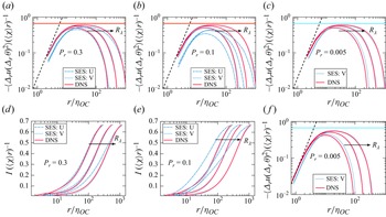
Mixed-structure functions for $Sc=1, {P_r}=0.3$
(a)
$Sc=1, {P_r}=0.3$
(a) $Sc=1, {P_r}=0.1$
(b) and
$Sc=1, {P_r}=0.1$
(b) and $Sc=1, {P_r}=0.005$
(c), and
$Sc=1, {P_r}=0.005$
(c), and $Sc=0.25, {P_r}=0.005$
(f). The horizontal line corresponds to 2/3. Forcing term
$Sc=0.25, {P_r}=0.005$
(f). The horizontal line corresponds to 2/3. Forcing term $I$
in (3.1) for
$I$
in (3.1) for $Sc=1$
and
$Sc=1$
and ${P_r}=0.3$
(d) and
${P_r}=0.3$
(d) and ${P_r}=0.1$
(e).
${P_r}=0.1$
(e).

3.2. Structure functions
A particularly important result for scalar mixing can be obtained from the Kármán–Howarth equation at high Péclet and Reynolds numbers in the inertial-convective range where dissipation, forcing and non-stationary effects can be neglected. This, known as the Yaglom’s relation (Yaglom Reference Yaglom1949), can be written as $\langle \varDelta _r u (\varDelta _r \theta )^2\rangle =-2\langle \chi \rangle r/3$
where
$\langle \varDelta _r u (\varDelta _r \theta )^2\rangle =-2\langle \chi \rangle r/3$
where $\varDelta _r \theta = \theta (x+r)-\theta (x)$
and
$\varDelta _r \theta = \theta (x+r)-\theta (x)$
and $\varDelta _r u = u(x+r)-u(x)$
where
$\varDelta _r u = u(x+r)-u(x)$
where $r$
is the separation along the direction of
$r$
is the separation along the direction of $u$
. This is the analogue to the four-fifth law for the velocity field (Kolmogorov Reference Kolmogorov1991). The mixed longitudinal structure function, normalised with
$u$
. This is the analogue to the four-fifth law for the velocity field (Kolmogorov Reference Kolmogorov1991). The mixed longitudinal structure function, normalised with $\langle \chi \rangle r$
is plotted in figure 2 (a,b,c) for
$\langle \chi \rangle r$
is plotted in figure 2 (a,b,c) for ${P_r}=0.3, 0.1, 0.005$
for
${P_r}=0.3, 0.1, 0.005$
for $Sc=1$
and figure 2(f) for
$Sc=1$
and figure 2(f) for ${P_r}=0.005$
and
${P_r}=0.005$
and $Sc=0.25$
.We see that small and large scales, especially for the V distribution, are closer to DNS than intermediate scales. This may not be surprising given that at small scales, the structure function is constrained by its analytical expansion for small separation distances, and forced scales are not affected by SES in our simulations. As expected, better agreement between SES and DNS is observed for higher
$Sc=0.25$
.We see that small and large scales, especially for the V distribution, are closer to DNS than intermediate scales. This may not be surprising given that at small scales, the structure function is constrained by its analytical expansion for small separation distances, and forced scales are not affected by SES in our simulations. As expected, better agreement between SES and DNS is observed for higher $P_r$
for the U distribution. The V distribution, on the other hand, remains very close to DNS and virtually unaffected by changes in
$P_r$
for the U distribution. The V distribution, on the other hand, remains very close to DNS and virtually unaffected by changes in $P_r$
for the range considered here. An increase in
$P_r$
for the range considered here. An increase in $R_\lambda$
(and
$R_\lambda$
(and $Sc$
, though to a lesser degree) brings the SES normalised mixed-structure function closer to
$Sc$
, though to a lesser degree) brings the SES normalised mixed-structure function closer to $2/3$
, the theoretical value predicted by Yaglom’s relation (horizontal line). To understand the origin of the difference between DNS and SES, we examine the transport equation that leads to the Yaglom relation, and contains the diffusive and forcing terms (Gotoh & Yeung Reference Gotoh and Yeung2012):
$2/3$
, the theoretical value predicted by Yaglom’s relation (horizontal line). To understand the origin of the difference between DNS and SES, we examine the transport equation that leads to the Yaglom relation, and contains the diffusive and forcing terms (Gotoh & Yeung Reference Gotoh and Yeung2012):
 \begin{equation} \langle \varDelta _r u(\varDelta _r \theta )^2\rangle =-2\langle \chi \rangle r/3 + 2D{\partial \langle (\varDelta _r \theta )^2 \rangle }/{\partial r} + {\mathcal I}. \end{equation}
where $\mathcal{I}$
represents the effect of forcing and unsteadiness. When divided by
$\mathcal{I}$
represents the effect of forcing and unsteadiness. When divided by $\langle \chi \rangle r$
, (3.1) can be written succinctly as
$\langle \chi \rangle r$
, (3.1) can be written succinctly as $2/3 = -A + B + I$
where
$2/3 = -A + B + I$
where $A$
is the normalised mixed-structure function,
$A$
is the normalised mixed-structure function, $B$
is the diffusion term, and
$B$
is the diffusion term, and $I$
is the non-dimensional
$I$
is the non-dimensional $\mathcal{I}$
. For long time averages in the inertial-convective range, the non-stationary and diffusion terms are small, making forcing the only other dominant effect (Iyer & Yeung Reference Iyer and Yeung2014). When forcing is negligible in the inertial-convective range, too, we recover Yaglom’s relation,
$\mathcal{I}$
. For long time averages in the inertial-convective range, the non-stationary and diffusion terms are small, making forcing the only other dominant effect (Iyer & Yeung Reference Iyer and Yeung2014). When forcing is negligible in the inertial-convective range, too, we recover Yaglom’s relation, $A=-2/3$
. In figure 2(d,e) we show this term for SES and DNS, for
$A=-2/3$
. In figure 2(d,e) we show this term for SES and DNS, for $Sc=1$
and
$Sc=1$
and ${P_r}=0.3,0.1$
. We can see that
${P_r}=0.3,0.1$
. We can see that $I$
for SES is different from DNS in the inertial-convective range. Its higher value for the U distribution and the balance equation (3.1) with
$I$
for SES is different from DNS in the inertial-convective range. Its higher value for the U distribution and the balance equation (3.1) with $D\approx 0$
explains the smaller magnitude of
$D\approx 0$
explains the smaller magnitude of $A$
seen in the other panels of figure 2. On the other hand,
$A$
seen in the other panels of figure 2. On the other hand, $I$
for the V distribution is almost identical to DNS, resulting in the same magnitude of
$I$
for the V distribution is almost identical to DNS, resulting in the same magnitude of $A$
in the other panels of figure 2. The value of this forcing-like effect due to the approximate nature of unresolved modes naturally increases with the number of these modes. For small
$A$
in the other panels of figure 2. The value of this forcing-like effect due to the approximate nature of unresolved modes naturally increases with the number of these modes. For small $r$
, a Taylor expansion yields
$r$
, a Taylor expansion yields $\langle \varDelta _r u (\varDelta _r \theta )^2\rangle /(\langle \chi \rangle r) \approx S_{u\theta }(r/\eta _{\textit{OC}})^2/(6\sqrt {15}\sqrt {Sc})$
(Yeung, Xu & Sreenivasan Reference Yeung, Xu and Sreenivasan2002), where the mixed gradient skewness
$\langle \varDelta _r u (\varDelta _r \theta )^2\rangle /(\langle \chi \rangle r) \approx S_{u\theta }(r/\eta _{\textit{OC}})^2/(6\sqrt {15}\sqrt {Sc})$
(Yeung, Xu & Sreenivasan Reference Yeung, Xu and Sreenivasan2002), where the mixed gradient skewness $S_{u\theta }$
represents the rate of production of
$S_{u\theta }$
represents the rate of production of $\chi$
due to the stretching of the scalar field by the turbulent strain field (Wyngaard Reference Wyngaard1971). It is negative and expected to approach an asymptotic value at high
$\chi$
due to the stretching of the scalar field by the turbulent strain field (Wyngaard Reference Wyngaard1971). It is negative and expected to approach an asymptotic value at high $R_\lambda$
, though the approach depends on flow details (Tang et al. Reference Tang, Antonia, Djenidi, Danaila and Zhou2016). In figure 2, both DNS and SES exhibit the predicted small-scale asymptote (dashed line), though with a vertical shift, indicating differences in the prefactor to the scaling law.
$R_\lambda$
, though the approach depends on flow details (Tang et al. Reference Tang, Antonia, Djenidi, Danaila and Zhou2016). In figure 2, both DNS and SES exhibit the predicted small-scale asymptote (dashed line), though with a vertical shift, indicating differences in the prefactor to the scaling law.
For scalar structure functions, Kolmogorov–Obukhov–Corrsin (KOC) phenomenology predicts $\langle (\varDelta _r \theta )^n \rangle \propto r^{n/3}$
in the inertial-convective range. In particular, for
$\langle (\varDelta _r \theta )^n \rangle \propto r^{n/3}$
in the inertial-convective range. In particular, for $n=2$
, the expression becomes
$n=2$
, the expression becomes $\langle (\varDelta _r \theta )^2 \rangle = C \langle \chi \rangle r^{2/3} \langle \epsilon \rangle ^{-1/3}$
corresponding to a
$\langle (\varDelta _r \theta )^2 \rangle = C \langle \chi \rangle r^{2/3} \langle \epsilon \rangle ^{-1/3}$
corresponding to a $k^{-5/3}$
scaling in Fourier space. The constant
$k^{-5/3}$
scaling in Fourier space. The constant $C$
has a value
$C$
has a value $\approx 1.6$
and is proportional to the Obukhov–Corrsin constant
$\approx 1.6$
and is proportional to the Obukhov–Corrsin constant $(C_{\textit{OC}})$
from the passive scalar spectrum (Iyer & Yeung Reference Iyer and Yeung2014). The compensated second-order structure function is shown in figures 3 (a,d,g,j). The excellent agreement at small scales for all values of
$(C_{\textit{OC}})$
from the passive scalar spectrum (Iyer & Yeung Reference Iyer and Yeung2014). The compensated second-order structure function is shown in figures 3 (a,d,g,j). The excellent agreement at small scales for all values of $P_r$
is unsurprising given the constraint imposed by Taylor expansion at the origin, yielding
$P_r$
is unsurprising given the constraint imposed by Taylor expansion at the origin, yielding $\langle (\varDelta _r \theta )^2 \rangle /( \langle \chi \rangle r^{2/3} \langle \epsilon \rangle ^{-1/3}) \approx (r/\eta _{\textit{OC}})^{4/3}/6$
. The effect of
$\langle (\varDelta _r \theta )^2 \rangle /( \langle \chi \rangle r^{2/3} \langle \epsilon \rangle ^{-1/3}) \approx (r/\eta _{\textit{OC}})^{4/3}/6$
. The effect of $P_r$
can be seen at larger
$P_r$
can be seen at larger $r$
, with increasing accuracy on increasing
$r$
, with increasing accuracy on increasing $P_r$
. For both Schmidt numbers, the overall shape of the structure function is consistent with DNS though some differences are seen in its normalised value in the inertial-convective range, which is larger for SES, especially for the U distribution. This, and the other observations in this section, can be explained as resulting from a distributed forcing originating from the SES modes. This force, (through
$P_r$
. For both Schmidt numbers, the overall shape of the structure function is consistent with DNS though some differences are seen in its normalised value in the inertial-convective range, which is larger for SES, especially for the U distribution. This, and the other observations in this section, can be explained as resulting from a distributed forcing originating from the SES modes. This force, (through $\mathcal I$
) stirs the scalar and also explains differences in the velocity field (Donzis & Sajeev Reference Donzis and Sajeev2024).
$\mathcal I$
) stirs the scalar and also explains differences in the velocity field (Donzis & Sajeev Reference Donzis and Sajeev2024).
Structure functions. (a–c) $Sc=1,P_r=0.3$
, (d–f)
$Sc=1,P_r=0.3$
, (d–f) $Sc=1,P_r=0.1$
, (g–i)
$Sc=1,P_r=0.1$
, (g–i) $Sc=1, P_r=0.005$
, (j–l)
$Sc=1, P_r=0.005$
, (j–l) $Sc=0.25, P_r=0.005$
. The green horizontal line in flatness plots correspond to 3.
$Sc=0.25, P_r=0.005$
. The green horizontal line in flatness plots correspond to 3.

Anisotropy and intermittency cause deviations from KOC predictions and are usually assessed via normalised high-order moments of increments: $\mu ^n_{\theta }(r)= {\langle (\varDelta _r \theta )^n\rangle } / {\langle (\varDelta _r \theta )^2\rangle ^{n/2}}$
. Non-universal and anisotropic signatures can be intuitively predicted for scalars forced with a mean gradient
$\mu ^n_{\theta }(r)= {\langle (\varDelta _r \theta )^n\rangle } / {\langle (\varDelta _r \theta )^2\rangle ^{n/2}}$
. Non-universal and anisotropic signatures can be intuitively predicted for scalars forced with a mean gradient ${\boldsymbol g}$
for which one can obtain, using dimensional arguments, a relation between odd and even moments:
${\boldsymbol g}$
for which one can obtain, using dimensional arguments, a relation between odd and even moments: $\langle (\varDelta _r\theta )^{2n+1} \rangle \propto ({\boldsymbol g}\boldsymbol\cdot \boldsymbol{r}) \langle (\varDelta _r\theta )^{2n} \rangle \propto r^{2n/3+1}$
in the inertial-convective range (Celani et al. Reference Celani, Lanotte, Mazzino and Vergassola2001). In homogeneous flows, odd-order structure functions (and thus
$\langle (\varDelta _r\theta )^{2n+1} \rangle \propto ({\boldsymbol g}\boldsymbol\cdot \boldsymbol{r}) \langle (\varDelta _r\theta )^{2n} \rangle \propto r^{2n/3+1}$
in the inertial-convective range (Celani et al. Reference Celani, Lanotte, Mazzino and Vergassola2001). In homogeneous flows, odd-order structure functions (and thus $\mu ^n_\theta (r)$
) vanish at large
$\mu ^n_\theta (r)$
) vanish at large $r$
. For small
$r$
. For small $r$
,
$r$
, $\mu ^n_\theta (r)$
tends to the normalised moments of scalar gradients (more later).The skewness of scalar increments,
$\mu ^n_\theta (r)$
tends to the normalised moments of scalar gradients (more later).The skewness of scalar increments, $\mu ^3_\theta (r)$
, is shown in figure 3 (b,e,h,k). The DNS and SES curves approach a non-zero asymptote at small
$\mu ^3_\theta (r)$
, is shown in figure 3 (b,e,h,k). The DNS and SES curves approach a non-zero asymptote at small $r$
, indicating a persistent anisotropy, expected for anisotropic forcing (Warhaft Reference Warhaft2000). While SES values are lower than DNS for the U distribution, results for the V distribution show much smaller deviations from DNS as seen in figure 3(b,e). As expected, increasing
$r$
, indicating a persistent anisotropy, expected for anisotropic forcing (Warhaft Reference Warhaft2000). While SES values are lower than DNS for the U distribution, results for the V distribution show much smaller deviations from DNS as seen in figure 3(b,e). As expected, increasing $P_r$
reduces these deviations. At intermediate
$P_r$
reduces these deviations. At intermediate $r$
, we see differences in the shape of
$r$
, we see differences in the shape of $\mu ^3_\theta (r)$
for different cases which is unsurprising given the differences in the stirring mechanism for each case (Donzis & Sajeev Reference Donzis and Sajeev2024). At large scales, as expected,
$\mu ^3_\theta (r)$
for different cases which is unsurprising given the differences in the stirring mechanism for each case (Donzis & Sajeev Reference Donzis and Sajeev2024). At large scales, as expected, $\mu ^3_\theta (r)$
tends to zero. In general, V cases are closer to the DNS than U cases since the stirring mechanism itself (
$\mu ^3_\theta (r)$
tends to zero. In general, V cases are closer to the DNS than U cases since the stirring mechanism itself ( $\mathcal I$
in (3.1)) is closer to DNS given the relatively larger fraction of low wavenumber modes that are evolved according to NS dynamics for V distributions.
$\mathcal I$
in (3.1)) is closer to DNS given the relatively larger fraction of low wavenumber modes that are evolved according to NS dynamics for V distributions.
Removing even a small fraction of modes from the dynamics of turbulence (as in decimation approaches (Lanotte et al. Reference Lanotte, Benzi, Malapaka, Toschi and Biferale2015)) has been shown to drastically quench intermittency. The SES velocity fields, on the other hand, remain intermittent even with just 10 % of NS modes (Donzis & Sajeev Reference Donzis and Sajeev2024). The effect on intermittency can be assessed from high-order structure functions, with order four shown in figure 3(c,f,i,l). For small $r$
,
$r$
, $\mu ^4_\theta (r)$
tends to the scalar gradient flatness and is seen to be greater than 3, indicating non-Gaussian intermittent behaviour. As the separation increases,
$\mu ^4_\theta (r)$
tends to the scalar gradient flatness and is seen to be greater than 3, indicating non-Gaussian intermittent behaviour. As the separation increases, $\mu ^4_\theta (r)$
falls to three as large scales become Gaussian. SES is able to retain this at small and large
$\mu ^4_\theta (r)$
falls to three as large scales become Gaussian. SES is able to retain this at small and large $r$
. There is remarkable agreement for U and V distributions for as low as 10 % and 0.5 % of modes, respectively, indicating that intermittency characteristics for scalars are not lost even when very few velocity modes obey strict NS dynamics. Scalar gradient flatness is known to depend on
$r$
. There is remarkable agreement for U and V distributions for as low as 10 % and 0.5 % of modes, respectively, indicating that intermittency characteristics for scalars are not lost even when very few velocity modes obey strict NS dynamics. Scalar gradient flatness is known to depend on $R_\lambda$
but is independent of Schmidt number for large
$R_\lambda$
but is independent of Schmidt number for large $Sc$
(Buaria et al. Reference Buaria, Clay, Sreenivasan and Yeung2021). Since
$Sc$
(Buaria et al. Reference Buaria, Clay, Sreenivasan and Yeung2021). Since $R_\lambda$
varies between simulations and the deviations could be an
$R_\lambda$
varies between simulations and the deviations could be an $R_\lambda$
effect, we compare moments appropriately normalised with
$R_\lambda$
effect, we compare moments appropriately normalised with $R_\lambda$
in the next section. On comparing normalised odd and even structure functions for the same
$R_\lambda$
in the next section. On comparing normalised odd and even structure functions for the same $P_r$
,
$P_r$
, $R_\lambda$
and
$R_\lambda$
and $Sc$
, we see that the even moments show better agreement with DNS. Since the stirring mechanism is different, this is not surprising, as some degree of universality has been observed in normalised even-order moments irrespective of the forcing technique (Gotoh & Watanabe Reference Gotoh and Watanabe2015). Odd-order moments, on the other hand, have a stronger dependence on forcing.
$Sc$
, we see that the even moments show better agreement with DNS. Since the stirring mechanism is different, this is not surprising, as some degree of universality has been observed in normalised even-order moments irrespective of the forcing technique (Gotoh & Watanabe Reference Gotoh and Watanabe2015). Odd-order moments, on the other hand, have a stronger dependence on forcing.
In summary, we see that, overall, to capture two-point statistics over the entire range of scales only a fraction of NS modes in the advecting velocity field appear to be necessary. Differences with DNS are explained by an additional distributed forcing due to SES modes.
3.3. Scalar gradient moments
Universality posits that small-scale properties such as gradients be statistically isotropic, regardless of the large scales. However, anisotropically forced passive scalar fields, such as those here with a mean scalar gradient ${\boldsymbol g}$
, remain anisotropic even at small scales. This anomalous behaviour is due to the presence of ‘ramp–cliff’ structures (Sreenivasan Reference Sreenivasan2019) which only form along the gradient. It is therefore common to study statistics of the scalar derivative along
${\boldsymbol g}$
, remain anisotropic even at small scales. This anomalous behaviour is due to the presence of ‘ramp–cliff’ structures (Sreenivasan Reference Sreenivasan2019) which only form along the gradient. It is therefore common to study statistics of the scalar derivative along ${\boldsymbol g}$
(typically termed the parallel scalar gradient,
${\boldsymbol g}$
(typically termed the parallel scalar gradient, $\boldsymbol\nabla _{\parallel} \theta$
) separate from the other directions. Small-scale anisotropy is typically observed by non-zero values of odd-order moments of
$\boldsymbol\nabla _{\parallel} \theta$
) separate from the other directions. Small-scale anisotropy is typically observed by non-zero values of odd-order moments of $\boldsymbol\nabla _{\parallel} \theta$
. Experimental and numerical data have shown that the skewness of
$\boldsymbol\nabla _{\parallel} \theta$
. Experimental and numerical data have shown that the skewness of $\boldsymbol\nabla _{\parallel} \theta$
remains
$\boldsymbol\nabla _{\parallel} \theta$
remains $\mathcal{O}(1)$
at high Reynolds numbers (Shete et al. Reference Shete, Boucher, Riley and de Bruyn Kops2022). This was observed even for Gaussian velocity fields, indicating scalar anisotropy does not originate from characteristics of the velocity field (Holzer & Siggia Reference Holzer and Siggia1994). Standardised odd-order moments of parallel scalar gradients,
$\mathcal{O}(1)$
at high Reynolds numbers (Shete et al. Reference Shete, Boucher, Riley and de Bruyn Kops2022). This was observed even for Gaussian velocity fields, indicating scalar anisotropy does not originate from characteristics of the velocity field (Holzer & Siggia Reference Holzer and Siggia1994). Standardised odd-order moments of parallel scalar gradients, $\sigma _{n}= {\langle (\boldsymbol\nabla _{\parallel} \theta )^n\rangle }/{\langle ( \boldsymbol\nabla _{\parallel} \theta )^2\rangle ^{n/2}}$
, have been found to scale with
$\sigma _{n}= {\langle (\boldsymbol\nabla _{\parallel} \theta )^n\rangle }/{\langle ( \boldsymbol\nabla _{\parallel} \theta )^2\rangle ^{n/2}}$
, have been found to scale with $R_\lambda$
and
$R_\lambda$
and $Sc$
as a power law for
$Sc$
as a power law for $Sc\gt 1$
, with values decreasing with
$Sc\gt 1$
, with values decreasing with $Sc$
for a fixed
$Sc$
for a fixed $R_\lambda$
. Since
$R_\lambda$
. Since $Sc \leqslant 1$
here, a power law in
$Sc \leqslant 1$
here, a power law in $Sc$
may not be discerned. As shown by Sreenivasan (Reference Sreenivasan2019); Buaria et al. (Reference Buaria, Clay, Sreenivasan and Yeung2021), these moments present more universal behaviour when normalised by
$Sc$
may not be discerned. As shown by Sreenivasan (Reference Sreenivasan2019); Buaria et al. (Reference Buaria, Clay, Sreenivasan and Yeung2021), these moments present more universal behaviour when normalised by ${R_\lambda }^{{(n-3)}/{2}}$
. Odd-order moments are shown in figure 4 for SES and DNS for different
${R_\lambda }^{{(n-3)}/{2}}$
. Odd-order moments are shown in figure 4 for SES and DNS for different $P_r$
and distributions. A slight but systematic trend with
$P_r$
and distributions. A slight but systematic trend with $P_r$
can be seen for the U distribution (blue and red symbols in figure 4
a,c). In particular we see a reduction in the magnitude of odd-order moments when
$P_r$
can be seen for the U distribution (blue and red symbols in figure 4
a,c). In particular we see a reduction in the magnitude of odd-order moments when $P_r$
decreases, indicating a reduction in anisotropy for fixed
$P_r$
decreases, indicating a reduction in anisotropy for fixed $Sc$
. The V distribution, on the other hand, is very close to DNS even with as low as 0.5 % resolved modes. The SES results seem to be independent of
$Sc$
. The V distribution, on the other hand, is very close to DNS even with as low as 0.5 % resolved modes. The SES results seem to be independent of $Sc$
for the range considered here.
$Sc$
for the range considered here.
Moments of parallel scalar gradient, normalised by $R_\lambda ^{(n-3)/2}$
, for
$R_\lambda ^{(n-3)/2}$
, for $n$
th order moment. Panels (a,c) correspond to odd-order moments
$n$
th order moment. Panels (a,c) correspond to odd-order moments $n=3, 5$
and (d,e) correspond to even-order moment
$n=3, 5$
and (d,e) correspond to even-order moment $n=4$
.
$n=4$
.

A flatness factor ( $\sigma _{4}$
) greater than 3, is indicative of non-Gaussianity and intermittency. From figure 4, we can see that SES moments are consistent with DNS again even with
$\sigma _{4}$
) greater than 3, is indicative of non-Gaussianity and intermittency. From figure 4, we can see that SES moments are consistent with DNS again even with ${P_r}=0.005$
. Since intermittency is stronger for parallel gradients, they provide a more stringent challenge for SES. We have indeed verified with our data that transverse gradients are better resolved and, therefore, not shown here.
${P_r}=0.005$
. Since intermittency is stronger for parallel gradients, they provide a more stringent challenge for SES. We have indeed verified with our data that transverse gradients are better resolved and, therefore, not shown here.
The PDF of normalised parallel scalar gradient $Z=\boldsymbol\nabla _{\parallel} \theta$
(a,b) and normalised scalar fluctuations (c,d). Colour lines correspond to SES U (
$Z=\boldsymbol\nabla _{\parallel} \theta$
(a,b) and normalised scalar fluctuations (c,d). Colour lines correspond to SES U ( ), SES V (
 ) and DNS (
 ). A Gaussian (dashed black line) is also included for reference.

3.4. Probability density functions (PDFs)
From normalised moments, we just concluded that the parallel scalar gradient is both anisotropic and intermittent. A more complete picture of the statistical behaviour of gradients can be obtained from their PDF. In figure 5(a,b) we show this PDF for ${R_\lambda }\approx 400$
and
${R_\lambda }\approx 400$
and $Sc=0.25,1$
for SES and DNS along with a Gaussian for comparison. Both the asymmetry and fat tails of the PDF are captured by SES, with just
$Sc=0.25,1$
for SES and DNS along with a Gaussian for comparison. Both the asymmetry and fat tails of the PDF are captured by SES, with just $0.5\,\%$
of NS modes. The SES tails for U distributions (dashed lines) are slightly less asymmetric than that of DNS (solid line). The V distribution (dashed–dotted lines) performs much better capturing the entire PDFs for extremely low
$0.5\,\%$
of NS modes. The SES tails for U distributions (dashed lines) are slightly less asymmetric than that of DNS (solid line). The V distribution (dashed–dotted lines) performs much better capturing the entire PDFs for extremely low $P_r$
which suggests that accurate NS dynamics at the large-velocity scales is necessary to capture mixing at the finest scales. Overall, we see that SES captures broadly both anisotropy and intermittency with as low as 0.5 % of resolved modes for low
$P_r$
which suggests that accurate NS dynamics at the large-velocity scales is necessary to capture mixing at the finest scales. Overall, we see that SES captures broadly both anisotropy and intermittency with as low as 0.5 % of resolved modes for low $Sc$
. Two small departures seen in the SES tails (especially for the U distribution) beyond 10 standard deviations are likely related to statistical convergence, given the non-systematic trend with
$Sc$
. Two small departures seen in the SES tails (especially for the U distribution) beyond 10 standard deviations are likely related to statistical convergence, given the non-systematic trend with $P_r$
. Similar behaviour is seen for the PDF of perpendicular scalar gradients (not included here since, as noted before, are better resolved than parallel gradients), which are known to be symmetric but less intermittent (Yeung et al. Reference Yeung, Xu and Sreenivasan2002). The PDF of the scalar fluctuation itself (
$P_r$
. Similar behaviour is seen for the PDF of perpendicular scalar gradients (not included here since, as noted before, are better resolved than parallel gradients), which are known to be symmetric but less intermittent (Yeung et al. Reference Yeung, Xu and Sreenivasan2002). The PDF of the scalar fluctuation itself ( $\theta$
) is shown in figure 5(c,d) for DNS and SES at
$\theta$
) is shown in figure 5(c,d) for DNS and SES at ${R_\lambda }=400$
and
${R_\lambda }=400$
and $Sc=0.25,1$
for different
$Sc=0.25,1$
for different $P_r$
. Since the flow becomes more intermittent at higher Reynolds number, we only present the PDF at the highest Reynolds number,
$P_r$
. Since the flow becomes more intermittent at higher Reynolds number, we only present the PDF at the highest Reynolds number, ${R_\lambda }=400$
, in our case. The PDFs at lower Reynolds number have similar behaviour and are hence not shown here.
${R_\lambda }=400$
, in our case. The PDFs at lower Reynolds number have similar behaviour and are hence not shown here.
In the presence of a mean scalar gradient, the PDF of the scalar itself is known to be approximately Gaussian with subGaussian tails (Gotoh & Watanabe Reference Gotoh and Watanabe2012). From figure 5(c,d), it can be seen that both SES and DNS are close to Gaussian for fluctuations within two or three standard deviations. The SES tails tends to be wider than DNS but there is no systematic trend with $P_r$
. The V results have narrower tails which are closer to DNS and perform slightly better than U results. Because of the well-known sensitivity of the tails to averaging windows (Watanabe & Gotoh Reference Watanabe and Gotoh2004) and the lack of a trend with
$P_r$
. The V results have narrower tails which are closer to DNS and perform slightly better than U results. Because of the well-known sensitivity of the tails to averaging windows (Watanabe & Gotoh Reference Watanabe and Gotoh2004) and the lack of a trend with $P_r$
, the differences seen in the far tails appear to be, in part, statistical.
$P_r$
, the differences seen in the far tails appear to be, in part, statistical.
Contours of the scalar field in the $x$
–
$x$
– $y$
plane normalised by
$y$
plane normalised by $\theta _{rms}$
at
$\theta _{rms}$
at ${R_\lambda } \approx 400$
and
${R_\lambda } \approx 400$
and $Sc=1$
. For reference the mean scalar gradient
$Sc=1$
. For reference the mean scalar gradient ${\boldsymbol g}$
is indicated in (a).
${\boldsymbol g}$
is indicated in (a).

Finally, in figure 6 we show some instantaneous contours of scalar fluctuations in an $x$
–
$x$
– $y$
plane for DNS, and SES with
$y$
plane for DNS, and SES with $P_r=0.005$
for V and
$P_r=0.005$
for V and $P_r=0.1$
for U. Consistent with the quantitative assessments presented earlier, the general structure of the scalar field, from large-scale structures to sharp contrasts over short distances especially in the
$P_r=0.1$
for U. Consistent with the quantitative assessments presented earlier, the general structure of the scalar field, from large-scale structures to sharp contrasts over short distances especially in the $x$
direction (‘ramp-cliffs’), is very well captured in the V simulation (figure 6
b) with only 0.5 % of NS modes. The U field (figure 6
c), on the other hand, presents some visually qualitative differences especially at the small scales where flow looks smoother than that from DNS. This is consistent with the smaller flatness factors for scalar gradients observed in figure 4.
$x$
direction (‘ramp-cliffs’), is very well captured in the V simulation (figure 6
b) with only 0.5 % of NS modes. The U field (figure 6
c), on the other hand, presents some visually qualitative differences especially at the small scales where flow looks smoother than that from DNS. This is consistent with the smaller flatness factors for scalar gradients observed in figure 4.
4. Discussion
A basic feature of turbulent flows is their wide range of scales, all of which have traditionally been thought to require obeying strict NS dynamics in order to describe the most important features of these flows. If one simply removes scales (typically represented by Fourier modes) from NS dynamics, a number of high-Reynolds-number features such as intermittency, disappear. It was recently shown, however, that these features are conserved when just 10 % of the modes obey NS dynamics while the others evolve according to trivial dynamics (Donzis & Sajeev Reference Donzis and Sajeev2024) in the so-called SES approach. Here we show that turbulent mixing also depends on a smaller set of velocity modes stirring a passive scalar. This was done by detailed comparisons between DNS and SES results for spectra, structure functions, and statistics of scalar and scalar gradients. For $Sc\le 1$
scalars, we found that just 0.5 % of appropriately distributed NS modes are sufficient to capture statistics of scalars and their gradients accurately. This is an interesting result given that while some universal features for scalars are expected based on classical phenomenology, theoretical analyses suggest that some features would depend on characteristics of the advecting velocity field (Kraichnan Reference Kraichnan1968).
$Sc\le 1$
scalars, we found that just 0.5 % of appropriately distributed NS modes are sufficient to capture statistics of scalars and their gradients accurately. This is an interesting result given that while some universal features for scalars are expected based on classical phenomenology, theoretical analyses suggest that some features would depend on characteristics of the advecting velocity field (Kraichnan Reference Kraichnan1968).
Comparing results from the uniform (U) and variable (V) distributions shed light on the relative importance of different velocity scales to turbulent mixing and can, thus, inform modelling approaches. Our results show that V distributions not only yield results closer to DNS than U distributions for the same $P_r$
, but can also capture scalar statistics at much lower values of
$P_r$
, but can also capture scalar statistics at much lower values of $P_r$
. This includes the energy spectra, structure functions and scalar gradient PDFs. Differences between the distributions are clear in the PDFs of scalar gradients where V distribution tails are indistinguishable from DNS. This may appear counterintuitive at first given that most of the contributions to scalar gradient moments are from small scalar scales and V distributions resolve more large and intermediate scales of the velocity field. This highlights the dynamic coupling between large velocity scales and small scalar scales. A phenomenological explanation of this coupling can be put forth by considering large velocity scales bringing together scalars of very different values. If this process happens at a time scale much shorter than diffusive processes, large scalar gradients are expected to form (Donzis & Yeung Reference Donzis and Yeung2010), leading to the observed intermittency for scalar gradients. The V distributions, with greater resolution at the large advecting scales, are therefore better able to capture the large-scale motions responsible for such events. Consistent with this view is the finding that the most intense scalar dissipation events (proportional to the square of scalar gradients) seem to be only weakly related to the smallest velocity scales where velocity gradients are strong (Schumacher, Sreenivasan & Yeung Reference Schumacher, Sreenivasan and Yeung2005).
$P_r$
. This includes the energy spectra, structure functions and scalar gradient PDFs. Differences between the distributions are clear in the PDFs of scalar gradients where V distribution tails are indistinguishable from DNS. This may appear counterintuitive at first given that most of the contributions to scalar gradient moments are from small scalar scales and V distributions resolve more large and intermediate scales of the velocity field. This highlights the dynamic coupling between large velocity scales and small scalar scales. A phenomenological explanation of this coupling can be put forth by considering large velocity scales bringing together scalars of very different values. If this process happens at a time scale much shorter than diffusive processes, large scalar gradients are expected to form (Donzis & Yeung Reference Donzis and Yeung2010), leading to the observed intermittency for scalar gradients. The V distributions, with greater resolution at the large advecting scales, are therefore better able to capture the large-scale motions responsible for such events. Consistent with this view is the finding that the most intense scalar dissipation events (proportional to the square of scalar gradients) seem to be only weakly related to the smallest velocity scales where velocity gradients are strong (Schumacher, Sreenivasan & Yeung Reference Schumacher, Sreenivasan and Yeung2005).
In Donzis & Sajeev (Reference Donzis and Sajeev2024) we have shown SES velocity fields obey NS dynamics as in DNS but with an additional broadband forcing term $(\hat {\boldsymbol{F}}_{\textit{SES}})$
. That is,
$(\hat {\boldsymbol{F}}_{\textit{SES}})$
. That is, $\hat{\boldsymbol{u}}_{n+1}= \hat{\boldsymbol{u}}_{n}+\Delta t {\mathcal L}(\hat{\boldsymbol{u}}) + \hat {\boldsymbol{F}}_{\textit{SES}}$
or
$\hat{\boldsymbol{u}}_{n+1}= \hat{\boldsymbol{u}}_{n}+\Delta t {\mathcal L}(\hat{\boldsymbol{u}}) + \hat {\boldsymbol{F}}_{\textit{SES}}$
or $\hat{\boldsymbol{u}}_{n+1}=\hat{\boldsymbol{u}}_{{uf},n+1}+\hat {\boldsymbol{F}}_{\textit{SES}}$
where
$\hat{\boldsymbol{u}}_{n+1}=\hat{\boldsymbol{u}}_{{uf},n+1}+\hat {\boldsymbol{F}}_{\textit{SES}}$
where $\hat{\boldsymbol{u}}_{{uf},n+1}$
is the velocity field without the additional broadband forcing and
$\hat{\boldsymbol{u}}_{{uf},n+1}$
is the velocity field without the additional broadband forcing and ${\mathcal L}(\hat{\boldsymbol{u}})$
represents the right-hand side of the NS equations. The distributed forcing
${\mathcal L}(\hat{\boldsymbol{u}})$
represents the right-hand side of the NS equations. The distributed forcing $\hat {\boldsymbol{F}}_\textit{SES}$
for the velocity field also appears in the scalar equation and compounds with the mean gradient term (
$\hat {\boldsymbol{F}}_\textit{SES}$
for the velocity field also appears in the scalar equation and compounds with the mean gradient term ( ${\boldsymbol g}$
) to form
${\boldsymbol g}$
) to form $-{\boldsymbol g}\boldsymbol\cdot (\hat{\boldsymbol{u}}_{{uf}} + \hat {\boldsymbol{F}}_{\textit{SES}}) -\hat {\boldsymbol{F}}_{\textit{SES}}*i {\boldsymbol k} \hat {\theta }$
. Many of the observed differences with DNS can be explained by considering the difference in forcing. These include different values of
$-{\boldsymbol g}\boldsymbol\cdot (\hat{\boldsymbol{u}}_{{uf}} + \hat {\boldsymbol{F}}_{\textit{SES}}) -\hat {\boldsymbol{F}}_{\textit{SES}}*i {\boldsymbol k} \hat {\theta }$
. Many of the observed differences with DNS can be explained by considering the difference in forcing. These include different values of $C_{\textit{OC}}$
, and the different trend towards the asymptotic Yaglom’s relation. It can also explain the observed decrease in anisotropy. The forcing term due to the mean scalar gradient is stronger at large scales, which is better resolved by the V distribution. As a result, the V distribution captures the anisotropy due to the forcing with greater accuracy. The U distribution, on the other hand, resolves less of the large scales, and thus the force, resulting in a reduction in the differences between directional statistics. This effect is further supported by the fact that reducing
$C_{\textit{OC}}$
, and the different trend towards the asymptotic Yaglom’s relation. It can also explain the observed decrease in anisotropy. The forcing term due to the mean scalar gradient is stronger at large scales, which is better resolved by the V distribution. As a result, the V distribution captures the anisotropy due to the forcing with greater accuracy. The U distribution, on the other hand, resolves less of the large scales, and thus the force, resulting in a reduction in the differences between directional statistics. This effect is further supported by the fact that reducing $P_r$
, which increases the effect of the additional forcing term, led to a reduction in anisotropy for the U distribution.
$P_r$
, which increases the effect of the additional forcing term, led to a reduction in anisotropy for the U distribution.
Finally, this work opens up many avenues for further studies. Given the success of SES in reproducing highly and moderately diffusive scalars ( $Sc \leqslant 1$
), it is natural to inquire about SES for weakly diffusive scalars (
$Sc \leqslant 1$
), it is natural to inquire about SES for weakly diffusive scalars ( $Sc\gt 1$
) for which important processes happen at subKolmogorov scales. The required distribution and percentage of NS modes in this regime can provide valuable insights into the dominant velocity scales. Additionally, one can investigate if the scalar field itself can be evolved using SES. This can especially be useful for high-
$Sc\gt 1$
) for which important processes happen at subKolmogorov scales. The required distribution and percentage of NS modes in this regime can provide valuable insights into the dominant velocity scales. Additionally, one can investigate if the scalar field itself can be evolved using SES. This can especially be useful for high- $Sc$
scalars whose resolution requirements are even more demanding than at moderate
$Sc$
scalars whose resolution requirements are even more demanding than at moderate $Sc$
. Lastly, many practical engineering applications involve scalar mixing in strained, anisotropic velocity fields where large and intermediate scales play an important role. A further study could assess the ability of SES to reproduce mixing statistics in such conditions.
$Sc$
. Lastly, many practical engineering applications involve scalar mixing in strained, anisotropic velocity fields where large and intermediate scales play an important role. A further study could assess the ability of SES to reproduce mixing statistics in such conditions.
Declaration of interests
The authors report no conflict of interest.




 Open access

