


1. Introduction
Hypersonic vehicles experience extreme heat loads during flight, which requires a suitable thermal management system to maintain material temperatures below critical thresholds (Anderson Reference Anderson2006). Heating results from a combination of heat conduction, radiation and gas–surface interactions. The complex nature of high-enthalpy flows interacting with the vehicle surface introduces uncertainties into predictive models. These interactions involve various processes, such as catalytic recombination, oxidation and nitridation, e.g. detailed in Prata, Minton & Schwartzentruber (Reference Prata, Minton and Schwartzentruber2021). In heterogeneous catalytic surface recombination, atomic species recombine on active surface sites, releasing heat into the material. These atomic species are adsorbed onto the surface and can react with other atoms – either adsorbed or in the gas phase – or with the surface material itself to form molecules that are then released into the flow (Josyula Reference Josyula2015). The material-dependent recombination effectiveness of atoms is typically described by the recombination coefficient,
 $\gamma$
. A comprehensive review of related experiments can be found in Chazot et al. (Reference Chazot, Panerai, Muylaert and Thoemel2010).
$\gamma$
. A comprehensive review of related experiments can be found in Chazot et al. (Reference Chazot, Panerai, Muylaert and Thoemel2010).
The catalytic recombination coefficient plays a significant role in surface heating and is often determined through experimentation. Massuti-Ballester & Herdrich (Reference Massuti-Ballester and Herdrich2021) present an extensive overview of experiments focused on oxygen and nitrogen recombination. Since the recombination coefficient is strongly influenced by surface temperature (Kim et al. Reference Kim, Yang, Park and Jo2021a ), experiments are conducted in high-enthalpy facilities that replicate the thermochemical conditions encountered during flight, including the high surface temperatures of the tested materials. To ensure accurate surface chemistry measurements, highly pure plasma flows are preferred, which can be achieved in inductively coupled plasma wind tunnels (Pidan et al. Reference Pidan, Auweter-Kurtz, Herdrich and Fertig2005; Meyers, Owens & Fletcher Reference Meyers, Owens and Fletcher2013; Viladegut Reference Viladegut2015). These facilities exhibit fluctuating behaviour, driven primarily by the characteristic frequency of their electrical power supply. Zander, Marynowski & Löhle (Reference Zander, Marynowski and Löhle2017) measured a dominant frequency of 300 Hz in the University of Stuttgart’s PWK3 facility, while Capponi et al. (Reference Capponi, Oldham, Konnik, Stephani, Bodony, Panesi, Elliott and Panerai2023) recorded a dominant frequency of 360 Hz in the University of Illinois’ Plasmatron X facility.
In addition to catalytic surface recombination, other surface reactions that occur during material ablation, such as surface oxidation and nitridation, are also influenced by the incoming flux of atomic particles and the properties of the surface. Ablation experiments are commonly conducted in plasma wind tunnels (Hermann et al. Reference Hermann, Löhle, Fasoulas, Leyland, Marraffa and Bouilly2017a ; Löhle et al. Reference Löhle, Hermann and Zander2018), where flow conditions can be highly unsteady, resulting in fluctuating free-stream conditions (Zander et al. Reference Zander, Marynowski and Löhle2017; Ravichandran et al. Reference Ravichandran, Leiser, Zander, Löhle, Matlovič, Tóth and Ferrière2021; Oldham et al. Reference Oldham, Capponi, Konnik, Stephani, Bodony, Panesi, Elliott and Panerai2023; Hermann & Chang Reference Hermann and Chang2024). These fluctuations can occur at frequencies of the order of several kHz, and the amplitudes can be significant (Hermann et al. Reference Hermann, Löhle, Fasoulas and Andrianatos2016; Zander, Hermann & Loehle Reference Zander, Hermann and Loehle2016). For example, Zander et al. (Reference Zander, Marynowski and Löhle2017) found that flow temperature in an inductively coupled plasma facility can fluctuate by as much as 4000 K, with a mean temperature of approximately 13 400 K. Similarly, Hermann & Chang (Reference Hermann and Chang2024) report temperature fluctuations of approximately 1300 K, with a mean temperature of 10 100 K in an arc-jet free stream.
While testing methodologies and flow characteristics may vary between different facilities, most suffer from some form of unsteadiness. Material samples tested under such conditions will be subjected to changing flow conditions – specifically, the boundary-layer-edge condition will be unsteady, leading to fluctuating surface conditions. As a result, the atomic mass flux to the surface will vary over time. If these experiments are analysed assuming steady-state conditions, errors may arise in the determination of material surface properties, as the dissociated flow physics and surface reaction efficiencies are non-linear. Furthermore, a varying heat flux will cause a fluctuation in surface temperature. Most gas–surface reactions are non-linearly related to the surface temperature (Prata et al. Reference Prata, Minton and Schwartzentruber2021). Through this non-linear behaviour, the average surface reactivity depends not only on the time-averaged atomic surface concentration, but also on its fluctuation magnitude. Therefore, it is desirable to develop a theory capable of predicting the strength of atomic-mass-fraction fluctuations at the surface for a non-equilibrium high-enthalpy flow. This allows for more accurate analysis of experiments, including the transient effects present in test facilities. Unsteady flows may simultaneously exhibit unsteadiness in other flow variables, such as density, velocity or temperature. This could lead to coupled effects, which are beyond the scope of the current work.
The aim of this paper is to develop a basic analytical theory for unsteady atomic and molecular species transport in reacting non-equilibrium boundary layers and to explore its properties. This allows the identification of relevant scaling parameters and the assessment of their respective significance for any given flow condition. The derivation of this approach is accomplished by constructing semi-empirical correlations based on analytical solutions to the reacting boundary-layer equations. It will be demonstrated that the unsteady reacting flow behaviour can be effectively described by a correlation that only requires knowledge of the steady frozen-flow solution and the fluctuation frequency. The current work builds upon the approximate theory developed by Inger (Reference Inger1963), extending it to account for unsteady flow dynamics. The resulting correlation is validated against fully coupled numerical solutions of the self-similar thermal and concentration boundary-layer equations. Under certain simplifying assumptions, the correlation can be expressed entirely in terms of non-dimensional heat and mass-transfer numbers. Finally, the paper highlights the impact of unsteady flow on the conditions faced in experimental ground testing facilities.
2. Analytical derivation
In this section, the governing equations and the strategy to solve them in a semi-empirical fashion are presented. The fully coupled boundary-layer theory of energy and species transport is broken down into two special cases, where either diffusion processes or chemical reactions dominate over other terms. This strategy allows for analytically closed solutions, supplemented by empirical correlations, which form the basis of a generalised engineering correlation describing unsteady non-equilibrium species transport.
Domain sketch of flow configuration (not to scale).

2.1. Governing equations
The assumption of a self-similar stagnation point around axisymmetric (
 $\epsilon = 1$
) or two-dimensional (
$\epsilon = 1$
) or two-dimensional (
 $\epsilon = 0$
) (
$\epsilon = 0$
) (
 $\epsilon$
is a shape parameter) bodies of revolution is employed, with the domain sketch presented in figure 1. In the following analysis, the subscript
$\epsilon$
is a shape parameter) bodies of revolution is employed, with the domain sketch presented in figure 1. In the following analysis, the subscript
 $\infty$
is used to denote properties of the free stream,
$\infty$
is used to denote properties of the free stream,
 $w$
is used to denote wall conditions, and
$w$
is used to denote wall conditions, and
 $e$
is used to denote boundary-layer-edge properties. The current work is limited to cases where self-similar theory is appropriate (see Harris & Ii Reference Harris and Ii1982; Tauber Reference Tauber1989; Prévereaud et al. Reference Prévereaud, Vérant and Annaloro2019). This includes the implicit assumption that the boundary-layer edge is in thermochemical equilibrium at all times (Goulard Reference Goulard1958). A body of spherical or cylindrical geometry is assessed as it represents a typical test configuration of material samples and diagnostic probes (Löhle et al. Reference Löhle, Hermann and Zander2018; Lewis et al. Reference Lewis, James, Ravichandran, Morgan and McIntyre2018). It also acts as a canonical geometry case, which can be used to transform the boundary-layer properties to other commonly used geometries in material testing, such as a flat-faced cylinder (Hermann et al. Reference Hermann, Löhle, Zander and Fasoulas2017b
). The unsteady boundary-layer equations of energy and atomic mass transport are considered. The derivation of Fay & Riddell (Reference Fay and Riddell1958) is adapted, utilising the formulation found in Inger (Reference Inger1963). These equations have been extended to include the appropriate unsteady terms, based on the derivation found in Dorrance (Reference Dorrance2017), yielding
$e$
is used to denote boundary-layer-edge properties. The current work is limited to cases where self-similar theory is appropriate (see Harris & Ii Reference Harris and Ii1982; Tauber Reference Tauber1989; Prévereaud et al. Reference Prévereaud, Vérant and Annaloro2019). This includes the implicit assumption that the boundary-layer edge is in thermochemical equilibrium at all times (Goulard Reference Goulard1958). A body of spherical or cylindrical geometry is assessed as it represents a typical test configuration of material samples and diagnostic probes (Löhle et al. Reference Löhle, Hermann and Zander2018; Lewis et al. Reference Lewis, James, Ravichandran, Morgan and McIntyre2018). It also acts as a canonical geometry case, which can be used to transform the boundary-layer properties to other commonly used geometries in material testing, such as a flat-faced cylinder (Hermann et al. Reference Hermann, Löhle, Zander and Fasoulas2017b
). The unsteady boundary-layer equations of energy and atomic mass transport are considered. The derivation of Fay & Riddell (Reference Fay and Riddell1958) is adapted, utilising the formulation found in Inger (Reference Inger1963). These equations have been extended to include the appropriate unsteady terms, based on the derivation found in Dorrance (Reference Dorrance2017), yielding
 \begin{equation} z'' + {\textit{Sc}}f(\eta ) z' - \frac {{\textit{Sc}}}{(1+\epsilon )\beta } \dot {z} = \frac {\alpha _e}{1 + \alpha _e} {\textit{Da}}\, R(z,\theta ) \end{equation}
and
 \begin{equation} \theta '' + {\textit{Pr}}f(\eta ) \theta ' - \frac {{\textit{Pr}}}{(1+\epsilon )\beta } \dot {\theta } = -\frac {\alpha _e}{1 + \alpha _e} {\textit{Da}}\, H_D \, R(z,\theta ), \end{equation}
with
 $z = \alpha / \alpha _e$
representing the non-dimensional atomic mass fraction, where
$z = \alpha / \alpha _e$
representing the non-dimensional atomic mass fraction, where
 $\alpha$
is the atomic mass fraction. Here
$\alpha$
is the atomic mass fraction. Here
 $\theta = T/T_e$
is the non-dimensional temperature,
$\theta = T/T_e$
is the non-dimensional temperature,
 ${\textit{Sc}}$
designates the Schmidt number,
${\textit{Sc}}$
designates the Schmidt number,
 $Pr$
the Prandtl number,
$Pr$
the Prandtl number,
 $f$
represents the Blasius function,
$f$
represents the Blasius function,
 $\beta = ({\rm d}u/{\rm d}s)$
is the stagnation-point velocity gradient, with
$\beta = ({\rm d}u/{\rm d}s)$
is the stagnation-point velocity gradient, with
 $s$
denoting the orientation tangential to the surface. The non-dimensional dissociation enthalpy is
$s$
denoting the orientation tangential to the surface. The non-dimensional dissociation enthalpy is
 $H_D = \alpha _e {Le}\, h_D / ( c_{p,M} T_e )$
,
$H_D = \alpha _e {Le}\, h_D / ( c_{p,M} T_e )$
,
 $Le$
is the Lewis number,
$Le$
is the Lewis number,
 $c_{p,M}$
is the specific heat at constant pressure of the molecules in the flow, and
$c_{p,M}$
is the specific heat at constant pressure of the molecules in the flow, and
 $h_D$
is the specific dissociation enthalpy of the molecules. A
$h_D$
is the specific dissociation enthalpy of the molecules. A
 $( \,\dot { }\, )$
symbol refers to the derivative with respect to time, and a (
$( \,\dot { }\, )$
symbol refers to the derivative with respect to time, and a (
 $'$
) symbol refers to a derivative with respect to the non-dimensional coordinate normal to the wall,
$'$
) symbol refers to a derivative with respect to the non-dimensional coordinate normal to the wall,
 \begin{equation} \eta = \sqrt {\frac {\rho _e(1+\epsilon ) \beta }{C \mu _e}} \int _0^y \frac {\rho }{\rho _e} {\rm d}y, \end{equation}
with the Chapman–Rubesin factor
 $C = \rho \mu / \rho _e \mu _e = {const}$
,
$C = \rho \mu / \rho _e \mu _e = {const}$
,
 $\rho$
is density, and
$\rho$
is density, and
 $\mu$
is dynamic viscosity. The Damkoehler number is
$\mu$
is dynamic viscosity. The Damkoehler number is
 \begin{equation} {\textit{Da}} = \frac {4 k_r^{\prime} T_e^{\xi - 2} {\textit{Sc}} }{ (1+\epsilon ) \beta } \left ( \frac {p_e}{R_u} \right )^2, \end{equation}
where the recombination rate constant
 $K_r$
relates to
$K_r$
relates to
 $k_r^{\prime} = K_r/T^\xi$
,
$k_r^{\prime} = K_r/T^\xi$
,
 $p_e$
represents the Pitot pressure and
$p_e$
represents the Pitot pressure and
 $R_u$
is the universal gas constant. The Damkoehler number gives a representation of the ratio of flow time over recombination time. In this work, the exponent for the reaction speed
$R_u$
is the universal gas constant. The Damkoehler number gives a representation of the ratio of flow time over recombination time. In this work, the exponent for the reaction speed
 $\xi =-1.5$
is used, according to the works of Fay & Riddell (Reference Fay and Riddell1958) and Dorrance (Reference Dorrance2017). In the current work, a generic mixture of atoms
$\xi =-1.5$
is used, according to the works of Fay & Riddell (Reference Fay and Riddell1958) and Dorrance (Reference Dorrance2017). In the current work, a generic mixture of atoms
 $A$
and diatomic molecules
$A$
and diatomic molecules
 $A_2$
are assumed where the dissociation and recombination reactions are described by
$A_2$
are assumed where the dissociation and recombination reactions are described by
 \begin{equation} A_2 + M \longleftrightarrow 2 A + M, \end{equation}
with the collision partner
 $M$
. This generic description is based on the work of Lighthill (Reference Lighthill1957) and was subsequently used by Fay & Riddell (Reference Fay and Riddell1958) in their analysis on stagnation-point heating. The approach lends itself to the current work, as a general theoretical framework is sought to be established applicable to different diatomic gases. The net reaction term
$M$
. This generic description is based on the work of Lighthill (Reference Lighthill1957) and was subsequently used by Fay & Riddell (Reference Fay and Riddell1958) in their analysis on stagnation-point heating. The approach lends itself to the current work, as a general theoretical framework is sought to be established applicable to different diatomic gases. The net reaction term
 $R$
is a function of both the local temperature and atom concentration and is calculated via the formulation found in Inger (Reference Inger1963):
$R$
is a function of both the local temperature and atom concentration and is calculated via the formulation found in Inger (Reference Inger1963):
 \begin{equation} R(z,\theta ) = \theta ^{\xi -2} \left ( \frac {1 + \alpha _e}{1 + \alpha _e z} \right ) \left ( z^2 - \frac {1 - \alpha _e^2 z^2}{1 - \alpha _e^2 } \exp \left ( -\frac {\theta _D}{\theta } \left ( 1 - \theta \right ) \right ) \right ), \end{equation}
where
 $\theta _D = h_D / (R_M T_e)$
is the dissociation temperature, and
$\theta _D = h_D / (R_M T_e)$
is the dissociation temperature, and
 $R_M$
is the specific gas constant of the molecules.
$R_M$
is the specific gas constant of the molecules.
Equations (2.1) and (2.2) are a coupled set of non-linear partial differential equations and require a numerical solution to accurately capture the flow behaviour in the boundary layer. The approach presented in this work is an approximation of these equations using analytical solutions of special cases and connecting these with an empirical correlation that captures the essential flow physics in unsteady reacting non-equilibrium boundary layers. This is achieved by investigating two simplified cases, the diffusion-dominated regime and the reaction-dominated regime. These two special cases will be derived in the following sections, followed by their application in a generalised correlation.
2.2. Diffusion-dominated regime
This special case considers a flow dominated by the effects of unsteady diffusion. Convective transport (
 ${\textit{Sc}}f(\eta ) z'$
) and reaction terms (
${\textit{Sc}}f(\eta ) z'$
) and reaction terms (
 $({\alpha _e}/{1 + \alpha _e}) {\textit{Da}}\, R(z,\theta )$
) are neglected. These simplifications allow a closed analytical solution to this case which is used in the following semi-empirical correlation. Equation (2.1) becomes
$({\alpha _e}/{1 + \alpha _e}) {\textit{Da}}\, R(z,\theta )$
) are neglected. These simplifications allow a closed analytical solution to this case which is used in the following semi-empirical correlation. Equation (2.1) becomes
 \begin{equation} z'' - \frac {{\textit{Sc}}}{(1+\epsilon )\beta } \dot {z} = 0. \end{equation}
This represents the boundary layer as a non-moving slab of fluid where reactions do not take place, i.e. frozen conditions (Wang, Yu & Bao (Reference Wang, Yu and Bao2018)). Neglecting convective transport has to be compensated by using an appropriate choice of boundary-layer thickness, which will be discussed in § 2.4. This formulation is used in part due to its linear time-invariant properties, allowing solutions to be superimposed. This property is exploited by employing the Fourier transform, yielding
 \begin{equation} \tilde {z}'' - \frac { {\rm i} \omega {\textit{Sc}}}{(1+\epsilon )\beta } \tilde {z} = 0, \end{equation}
where
 $\tilde {z}$
is the Fourier-transformed non-dimensional concentration and
$\tilde {z}$
is the Fourier-transformed non-dimensional concentration and
 $\omega$
is a frequency. A general solution to (2.8) is
$\omega$
is a frequency. A general solution to (2.8) is
 \begin{equation} \tilde {z}= C_1\, \exp \left ( \left ( 1+ {\rm i} \right ) \sqrt {\frac {\omega \,{\textit{Sc}}}{2 (1+\epsilon )\beta }}\, \eta \right ) + C_2\, \exp \left ( - \left ( 1+ {\rm i} \right ) \sqrt {\frac {\omega \,{\textit{Sc}}}{2 (1+\epsilon )\beta }} \, \eta \right ), \end{equation}
where the coefficients
 $C_{1,2}$
are calculated based on the boundary conditions
$C_{1,2}$
are calculated based on the boundary conditions
 \begin{equation} z(\delta _c) = 1 + \Delta z_\infty \, \cos (\omega t);\,\,\,\,\,\,\,\,\,\,\,\, z'(0)= \sigma z(0). \end{equation}
The first term in (2.10) describes the conditions found at the edge of the concentration boundary layer thickness at
 $\eta = \delta _c$
. A harmonic oscillation of frequency
$\eta = \delta _c$
. A harmonic oscillation of frequency
 $\omega$
and amplitude
$\omega$
and amplitude
 $\Delta z_\infty$
is imposed originating from concentration fluctuations in the free stream. A single frequency is investigated, as arbitrary time-dependent boundary-layer fluctuations can be decomposed into a range of frequencies via Fourier analysis. The linear nature of the investigated problem allows their superposition, not restricting the generality of boundary-layer-edge fluctuation conditions. These unsteady fluctuations could occur due to electrical power supplies varying in input power, turbulent fluctuations in the flow, flow entrainment and large scale eddies, etc. (Hermann et al. Reference Hermann, Löhle, Fasoulas and Andrianatos2016; Capponi et al. Reference Capponi, Padovan, Elliott, Panesi, Bodony and Panerai2024). The boundary-layer profile will consist of a steady-state mean profile and a superimposed oscillating component, due to the linearity of (2.8). The employed solution (2.9) considers only the transient behaviour and omits the superimposed steady-state contribution. This simplifies the solution slightly and does not restrict the generality of the approach. Additionally, this simplifies the boundary-layer-edge condition to
$\Delta z_\infty$
is imposed originating from concentration fluctuations in the free stream. A single frequency is investigated, as arbitrary time-dependent boundary-layer fluctuations can be decomposed into a range of frequencies via Fourier analysis. The linear nature of the investigated problem allows their superposition, not restricting the generality of boundary-layer-edge fluctuation conditions. These unsteady fluctuations could occur due to electrical power supplies varying in input power, turbulent fluctuations in the flow, flow entrainment and large scale eddies, etc. (Hermann et al. Reference Hermann, Löhle, Fasoulas and Andrianatos2016; Capponi et al. Reference Capponi, Padovan, Elliott, Panesi, Bodony and Panerai2024). The boundary-layer profile will consist of a steady-state mean profile and a superimposed oscillating component, due to the linearity of (2.8). The employed solution (2.9) considers only the transient behaviour and omits the superimposed steady-state contribution. This simplifies the solution slightly and does not restrict the generality of the approach. Additionally, this simplifies the boundary-layer-edge condition to
 $ z(\delta _c) = \Delta z_\infty \cos (\omega t)$
. At the wall, a material with catalytic recombination coefficient
$ z(\delta _c) = \Delta z_\infty \cos (\omega t)$
. At the wall, a material with catalytic recombination coefficient
 $\gamma$
is assumed to be present. The factor
$\gamma$
is assumed to be present. The factor
 $\sigma$
relates to this via
$\sigma$
relates to this via
 \begin{equation} \sigma = \frac { {\textit{Sc}} \, K_w }{\mu _w} \sqrt {\frac {2 C \rho _e \mu _e}{(1+\epsilon ) \beta }}, \end{equation}
where
 $\mu$
is the dynamic viscosity,
$\mu$
is the dynamic viscosity,
 $\rho$
is the density, and
$\rho$
is the density, and
 $K_w$
is the speed of atom recombination at the surface,
$K_w$
is the speed of atom recombination at the surface,
 \begin{equation} K_w = \gamma \sqrt {R_M T_w / \pi }. \end{equation}
The factor
 $\sigma$
can be interpreted as an inverse non-dimensional length scale, denoted as
$\sigma$
can be interpreted as an inverse non-dimensional length scale, denoted as
 \begin{equation} l_w = \frac {1}{\sigma }. \end{equation}
Fully catalytic surface conditions (all incoming atoms recombine) results in a very small
 $l_w$
, while non-catalytic conditions result in an infinity large
$l_w$
, while non-catalytic conditions result in an infinity large
 $l_w$
.
$l_w$
.
The goal of the following analysis is to relate the fluctuation amplitude at the wall
 $\Delta z_w$
to the fluctuation amplitude at the boundary-layer edge
$\Delta z_w$
to the fluctuation amplitude at the boundary-layer edge
 $\Delta z_\infty$
. To simplify solution (2.9), all terms including
$\Delta z_\infty$
. To simplify solution (2.9), all terms including
 $\textrm i$
are dropped, as they do not contribute to the amplitude change, but describe the time-dependent behaviour. This yields for the oscillation amplitudes,
$\textrm i$
are dropped, as they do not contribute to the amplitude change, but describe the time-dependent behaviour. This yields for the oscillation amplitudes,
 \begin{equation} \tilde {\Delta} z(\eta ) = \tilde {\Delta} z_\infty \frac { \left ( 1/\delta _S + 1/l_w \right ) \exp \left ( \eta /\delta _S \right ) + \left ( 1/\delta _S - 1/l_w \right ) \exp \left ( -\eta /\delta _S \right ) }{ \left ( 1/\delta _S + 1/l_w \right ) \exp \left ( \delta _c/\delta _S \right ) + \left ( 1/\delta _S - 1/l_w \right ) \exp \left ( -\delta _c/\delta _S \right ) }. \end{equation}
For the fluctuation amplitude at the wall
 $(\eta =0)$
, this simplifies to
$(\eta =0)$
, this simplifies to
 \begin{equation} \frac {\tilde {\Delta} z_w}{\tilde {\Delta} z_\infty } = \frac {\Delta z_w}{\Delta z_\infty } = 2 \left [ \left ( 1 + \frac {\delta _S}{l_w} \right ) \exp \left ( \frac {\delta _c}{\delta _S} \right ) + \left ( 1 - \frac {\delta _S}{l_w} \right ) \exp \left ( -\frac {\delta _c}{\delta _S} \right ) \right ]^{-1} , \end{equation}
with
 \begin{equation} \delta _S = \sqrt {\frac {2 (1+\epsilon )\beta }{\omega \,{\textit{Sc}}}}, \end{equation}
which can be interpreted as the Stokes-layer thickness of an unsteady concentration problem. This is analogous to other Stokes layers of oscillating transport phenomena, such as momentum and heat (Pal & Chakraborty Reference Pal and Chakraborty2015; Schlichting & Gersten Reference Schlichting and Gersten2017). The Stokes-layer thickness describes a measure for the penetration depth of a wave with frequency
 $\omega$
. As the frequency increases, the diffusive inertia of the medium will attenuate the propagation of this wave, decreasing its penetration depth (Hermann Reference Hermann2025). Equation (2.15) describes the relative amplitude of a concentration fluctuation of frequency
$\omega$
. As the frequency increases, the diffusive inertia of the medium will attenuate the propagation of this wave, decreasing its penetration depth (Hermann Reference Hermann2025). Equation (2.15) describes the relative amplitude of a concentration fluctuation of frequency
 $\omega$
at the wall. For the case of
$\omega$
at the wall. For the case of
 $\omega = 0$
, the Stokes-layer thickness
$\omega = 0$
, the Stokes-layer thickness
 $\delta _S$
becomes infinite, yielding the limiting solution of (2.15) as
$\delta _S$
becomes infinite, yielding the limiting solution of (2.15) as
 \begin{equation} \lim _{\delta _S \to \infty } \frac {\Delta z_w}{\Delta z_\infty } = \frac {1}{1 + \frac {\delta _c}{l_w}}. \end{equation}
The solution (2.15) relies on the specification of a mass diffusion boundary-layer thickness
 $\delta _c$
, representing the interface between boundary layer and inviscid external flow. This boundary-layer thickness is defined in relation to the thermal boundary layer, analogous to Hermann (Reference Hermann2025). In this work, the conduction length,
$\delta _c$
, representing the interface between boundary layer and inviscid external flow. This boundary-layer thickness is defined in relation to the thermal boundary layer, analogous to Hermann (Reference Hermann2025). In this work, the conduction length,
 \begin{equation} \delta _{T,L} = \frac {1 - \theta _w}{ \left ( \frac {\partial \theta }{\partial \eta }\right )_w } \end{equation}
is considered alongside the thermal-boundary-layer thickness,
 \begin{equation} \delta _{T,T} = 2 \frac {1 - \theta _w}{ \left ( \frac {\partial \theta }{\partial \eta }\right )_w }. \end{equation}
Here
 $\delta _{T,L}$
represents the thickness required for a solid medium to conduct the same heat flux as the boundary layer (Smith & Spalding Reference Smith and Spalding1958; Smith Reference Smith1979);
$\delta _{T,L}$
represents the thickness required for a solid medium to conduct the same heat flux as the boundary layer (Smith & Spalding Reference Smith and Spalding1958; Smith Reference Smith1979);
 $\delta _{T,T}$
, instead, represents the thermal-boundary-layer thickness required to fulfil the Reynolds analogy for Prandtl numbers close to unity, if a Pohlhausen velocity–boundary-layer profile is present (Schlichting & Gersten Reference Schlichting and Gersten2017). Using the correlation between mass diffusion and thermal boundary-layer thicknesses found in Dorrance (Reference Dorrance2017) for a Prandtl number close to unity, the diffusion boundary layer is calculated as
$\delta _{T,T}$
, instead, represents the thermal-boundary-layer thickness required to fulfil the Reynolds analogy for Prandtl numbers close to unity, if a Pohlhausen velocity–boundary-layer profile is present (Schlichting & Gersten Reference Schlichting and Gersten2017). Using the correlation between mass diffusion and thermal boundary-layer thicknesses found in Dorrance (Reference Dorrance2017) for a Prandtl number close to unity, the diffusion boundary layer is calculated as
 \begin{equation} \delta _c = \frac {\delta _T}{ \sqrt { {Le}}}, \end{equation}
where
 $\delta _T$
is determined by either (2.18) or (2.19). A schematic of a typical boundary-layer profile is provided in figure 2, which illustrates the considered length scales. Equation (2.15) developed in this section can be interpreted as a frequency-resolved impulse response of the boundary layer to a change in external flow conditions, if diffusion is the dominant transport mechanism. This approach allows the use of Duhamel’s theorem to superimpose solutions based on arbitrary boundary-layer-edge fluctuations.
$\delta _T$
is determined by either (2.18) or (2.19). A schematic of a typical boundary-layer profile is provided in figure 2, which illustrates the considered length scales. Equation (2.15) developed in this section can be interpreted as a frequency-resolved impulse response of the boundary layer to a change in external flow conditions, if diffusion is the dominant transport mechanism. This approach allows the use of Duhamel’s theorem to superimpose solutions based on arbitrary boundary-layer-edge fluctuations.
Schematic of boundary-layer atomic concentration profile, with characteristic length scales of diffusion problem.

2.3. Reaction-dominated regime
In this regime, the rate of atomic consumption through recombination reactions is far higher than the local rate of change, i.e. the storage term
 $({{\textit{Sc}}}/{(1+\epsilon )\beta }) \dot {z}$
is small compared with the reaction term
$({{\textit{Sc}}}/{(1+\epsilon )\beta }) \dot {z}$
is small compared with the reaction term
 $({\alpha _e}/{1 + \alpha _e}) {\textit{Da}}\, R(z,\theta )$
. Equation (2.1) is simplified to
$({\alpha _e}/{1 + \alpha _e}) {\textit{Da}}\, R(z,\theta )$
. Equation (2.1) is simplified to
 \begin{equation} z'' + {\textit{Sc}}f z' = \frac {\alpha _e}{1 + \alpha _e} {\textit{Da}}\, R(z,\theta ) \end{equation}
resulting in a quasi-steady solution of the boundary layer. These solutions assume that the influence of boundary-layer-edge conditions is instantaneously transported to the wall. In this case, boundary conditions are
 \begin{equation} z(\delta _c) = 1 ;\,\,\,\,\,\,\,\,\,\,\,\, z'(0)= \sigma z(0) \end{equation}
for nominal conditions without external fluctuations, and
 \begin{equation} z(\delta _c) = 1 + \Delta z_\infty ;\,\,\,\,\,\,\,\,\,\,\,\, z'(0)= \sigma z(0) \end{equation}
for perturbed conditions with perturbation magnitude
 $\Delta z_\infty$
. These conditions are identical to the case used in (2.10), apart from dropping the oscillation term. This is due to the fact that an instantaneous transport is assumed, and the temporal rate of change of boundary-layer-edge conditions therefore becomes irrelevant. Extending the work of Inger (Reference Inger1963), a solution to (2.21) is achieved by double integration of (2.21) with an integrating factor of
$\Delta z_\infty$
. These conditions are identical to the case used in (2.10), apart from dropping the oscillation term. This is due to the fact that an instantaneous transport is assumed, and the temporal rate of change of boundary-layer-edge conditions therefore becomes irrelevant. Extending the work of Inger (Reference Inger1963), a solution to (2.21) is achieved by double integration of (2.21) with an integrating factor of
 $\exp ( {\textit{Sc}} \int _{0}^{\eta } f \mathrm {d}\eta )$
, yielding
$\exp ( {\textit{Sc}} \int _{0}^{\eta } f \mathrm {d}\eta )$
, yielding
 \begin{equation} z(\eta ) = z_F(\eta ) - \frac {\alpha _e}{1 + \alpha _e} {\textit{Da}} \left ( \frac {z_F(\eta )}{z_F(\delta _c)} g(\delta _c) - g(\eta ) \right ) \end{equation}
with
 \begin{equation} g(\eta ) = \int _{0}^{\eta } \exp \left ( - {\textit{Sc}} \int _{0}^{\eta } f \mathrm {d}\eta \right )\left ( \int _{0}^{\eta } \exp \left ( {\textit{Sc}} \int _{0}^{\eta } f \mathrm {d}\eta \right ) R \mathrm {d}\eta \right ) \mathrm {d}\eta , \end{equation}
where
 $z_F$
refers to the frozen boundary-layer profile,
$z_F$
refers to the frozen boundary-layer profile,
 $g$
is a boundary layer integral factor, i.e. the solution of the ordinary differential equation
$g$
is a boundary layer integral factor, i.e. the solution of the ordinary differential equation
 \begin{equation} z_F'' + {\textit{Sc}}f z_F' = 0, \end{equation}
where the boundary conditions (2.22) and (2.23) also apply to this case. The frozen-wall condition can be determined analytically using Goulard (Reference Goulard1958), by employing a double integration, yielding
 \begin{equation} z_F(0) = \frac {z_F(\delta _c)}{\sigma I(\delta _c) + 1} \end{equation}
with
 \begin{equation} I(\delta _c) = \int _{0}^{\delta _c} \exp \left ( - {\textit{Sc}} \int _{0}^{\delta _c} f \mathrm {d}\eta \right ) \mathrm {d}\eta . \end{equation}
The integral can be transformed slightly into a new non-dimensional spatial domain
 $\tilde {\eta } = \eta / \delta _c$
which equals to unity at the boundary-layer edge:
$\tilde {\eta } = \eta / \delta _c$
which equals to unity at the boundary-layer edge:
 \begin{equation} \tilde {I} = \int _{0}^{1} \delta _c \,\exp \left ( - {\textit{Sc}} \int _{0}^{1} f \mathrm {d}\tilde {\eta } \right ) \mathrm {d}\tilde {\eta } = I(\delta _c) /\delta _c. \end{equation}
This normalisation is conducted to non-dimensionalise the derived solution. Evaluating (2.24) at the wall (
 $\eta =0$
) with the nominal (unperturbed) boundary condition
$\eta =0$
) with the nominal (unperturbed) boundary condition
 $z_F(\delta _c) = 1$
yields
$z_F(\delta _c) = 1$
yields
 \begin{equation} z(0) = z_F(0) \left ( 1 - \frac {\alpha _e}{1 + \alpha _e} {\textit{Da}} \, g(\delta _c) \right ). \end{equation}
Using the perturbed boundary condition
 $z_F(\delta _c) = 1 +\Delta z_\infty$
to denote the increase of external concentration by the relative fraction
$z_F(\delta _c) = 1 +\Delta z_\infty$
to denote the increase of external concentration by the relative fraction
 $\Delta z_\infty$
, yields the solution
$\Delta z_\infty$
, yields the solution
 \begin{equation} z^\Delta (0) = z_F^\Delta (0) \left ( 1 - \frac {\alpha _e}{(1 + \alpha _e) (1 + \Delta z_\infty )} {\textit{Da}} \, g^\Delta (\delta _c) \right ). \end{equation}
Quantities denoted by (
 $^\Delta$
) relate to boundary conditions (2.23), while all other cases refer to boundary conditions (2.22). Utilising (2.27) and (2.29) yields
$^\Delta$
) relate to boundary conditions (2.23), while all other cases refer to boundary conditions (2.22). Utilising (2.27) and (2.29) yields
 \begin{equation} z_F(0) = \frac {1}{\frac {\delta _c}{l_w} \tilde {I} + 1} \,\,\,\,\,\,\, \mathrm{and} \,\,\,\,\,\,\, z_F^\Delta (0) = \frac {1+\Delta z_\infty }{\frac {\delta _c}{l_w} \tilde {I} + 1}. \end{equation}
Using this, the difference between (2.30) and (2.31), corresponding to the difference in wall concentration for a given boundary-layer-edge concentration perturbation of
 $\Delta z_\infty$
, is
$\Delta z_\infty$
, is
 \begin{equation} \Delta z_w = z^\Delta (0) - z(0) = z_F(0) \left ( \Delta z_\infty - \frac {\alpha _e}{(1 + \alpha _e)} {\textit{Da}} \, \left ( g^\Delta (\delta _c) - g(\delta _c) \right ) \right ). \end{equation}
The
 $g$
-integrals, given with (2.25), are an implicit function of
$g$
-integrals, given with (2.25), are an implicit function of
 $z$
, which would require an iterative solution to (2.33). To avoid this recursive solution procedure, an empirical correlation is proposed. It has been found that the approximation
$z$
, which would require an iterative solution to (2.33). To avoid this recursive solution procedure, an empirical correlation is proposed. It has been found that the approximation
 \begin{equation} \frac {\alpha _e}{(1 + \alpha _e)} {\textit{Da}} \, \left ( g^\Delta (\delta _c) - g(\delta _c) \right ) \approx \Delta z_\infty \left ( 1 - \frac {z(0)}{z_F(0)} \right ) \end{equation}
gives a satisfactory prediction of the difference between the two integral terms. The accuracy is better than 10.4 % for all investigated cases in this work (see § 3.2 for details). The fraction
 $z(0) / z_F(0)$
is mainly a function of Damkoehler number, and can be calculated by solving the nonlinear ordinary differential (2.21) to obtain
$z(0) / z_F(0)$
is mainly a function of Damkoehler number, and can be calculated by solving the nonlinear ordinary differential (2.21) to obtain
 $z(0)$
, and utilising (2.32) for
$z(0)$
, and utilising (2.32) for
 $z_F(0)$
. Alternatively, this ratio can be determined analytically using Inger (Reference Inger1963) which utilises only steady-state frozen solutions, which is more in keeping with the approach taken in this work. Either way, the final solution for the wall concentration change under quasi-steady conditions is
$z_F(0)$
. Alternatively, this ratio can be determined analytically using Inger (Reference Inger1963) which utilises only steady-state frozen solutions, which is more in keeping with the approach taken in this work. Either way, the final solution for the wall concentration change under quasi-steady conditions is
 \begin{equation} \Delta z_w = \Delta z_\infty \frac { \frac {z(0)}{z_F(0)} }{\frac {\delta _c}{l_w} \tilde {I} + 1 } = \Delta z_\infty \, z(0). \end{equation}
The special cases of diffusion- and reaction-dominated regimes build the basis of the generalised correlation derived in this work, which is presented in the following.
2.4. Generalised correlation
The hypothesis utilised in the current work is based on the assumption that effects due to chemical reactions are separable from diffusion. This allows the formulation of a general correlation:
 \begin{equation} \frac {\Delta z_w}{\Delta z_\infty } = F_{\textit{Diff.}} \boldsymbol{\cdot }G_{\textit{Chem.}}, \end{equation}
where
 $F_{\textit{Diff.}}$
describes the attenuation of fluctuations due to the inertia of boundary-layer mass transport, and
$F_{\textit{Diff.}}$
describes the attenuation of fluctuations due to the inertia of boundary-layer mass transport, and
 $G_{\textit{Chem.}}$
describes the suppression of fluctuations due to chemical reactions, foremost recombination. The variable
$G_{\textit{Chem.}}$
describes the suppression of fluctuations due to chemical reactions, foremost recombination. The variable
 $F_{\textit{Diff.}}$
utilises (2.15) normalised by its limit for
$F_{\textit{Diff.}}$
utilises (2.15) normalised by its limit for
 $\omega = 0$
, given in (2.17), leading to
$\omega = 0$
, given in (2.17), leading to
 \begin{equation} A = \frac {\frac {\Delta z_w}{\Delta z_\infty }|_{\textit{Diff.}} }{ \lim _{\delta _S \to \infty } \frac {\Delta z_w}{\Delta z_\infty }|_{\textit{Diff.}} } = \frac { 2 + 2 \frac {\delta _c}{l_w} }{ \left ( 1 + \frac {\delta _S}{l_w} \right ) \exp \left ( \frac {\delta _c}{\delta _S} \right ) + \left ( 1 - \frac {\delta _S}{l_w} \right ) \exp \left ( -\frac {\delta _c}{\delta _S} \right ) } . \end{equation}
This function describes the attenuation of mass transport relative to the maximum possible wall value. It is further used to define
 \begin{equation} F_{\textit{Diff.}} = A \left ( \delta _{T,L} \right ) - \frac { A\left ( \delta _{T,L} \right ) - A\left ( \delta _{T,T} \right ) }{ 1 + 8.2 \left ( \frac {{\textit{Sc}} \omega }{ \beta (1+\epsilon ) } \right )^{-3} } . \end{equation}
Equation (2.38) utilises an empirical correlation which is based on the data analysis presented in § 3.1, where respective details are discussed in greater depth. It utilises the definitions in (2.18) and (2.19) for the thermal boundary-layer thickness, which in turn determine the concentration boundary-layer thickness through (2.20). This is finally used in (2.37).
The second term in (2.36), describing wall concentration attenuation due to chemical reactions utilises (2.35):
 \begin{equation} G_{\textit{Chem.}} = \frac { \frac {z(0)}{z_F(0)} }{\frac {\delta _c}{l_w} \tilde {I} + 1 } , \end{equation}
resulting in the full correlation
 \begin{equation} \frac {\Delta z_w}{\Delta z_\infty } = \left [ A \left ( \delta _{T,L} \right ) - \frac { A\left ( \delta _{T,L} \right ) - A\left ( \delta _{T,T} \right ) }{ 1 + 8.2 \left ( \frac {{\textit{Sc}} \omega }{ \beta (1+\epsilon ) } \right )^{-3} } \right ] \left [ \frac { \frac {z(0)}{z_F(0)} }{\frac {\delta _c}{l_w} \tilde {I} + 1 } \right ]. \end{equation}
The correlation features a few noteworthy properties that give insight into the behaviour of the fluid mechanics. All functions involved are only dependent on the steady-state frozen boundary-layer solution, which can be readily obtained using either simple numerical simulations or classical theory (Goulard Reference Goulard1958; Dorrance Reference Dorrance2017). Another useful aspect is that this correlation retains the linear time-invariant property found in § 2.2. As such, this approach can be viewed as an approximate linearisation of the inherently nonlinear flow physics. The linear time-invariant property allows the calculation of a frequency-resolved impulse response which can then be applied to arbitrary temporal boundary conditions at the boundary-layer edge using Duhamel’s theorem.
Furthermore, several special cases exist for components in correlation (2.40) that lead to substantial simplification. These are (i) either very fast or slow flow oscillations, (ii) fully or non-catalytic surface behaviour and (iii) frozen or fully equilibrated flow. The diffusion term
 $A$
depends only on the catalytic and frequency aspects and can be simplified as follows.
$A$
depends only on the catalytic and frequency aspects and can be simplified as follows.
High frequency (small
 $\delta _S$
) and fully catalytic wall (small
$\delta _S$
) and fully catalytic wall (small
 $l_w$
):
$l_w$
):
 \begin{equation} \lim _{\delta _S \to 0, \,\, l_w \to 0} A = \frac { \frac {\delta _c}{l_w} }{ \mathrm{sinh} \left (\frac {\delta _c}{\delta _S} \right ) } . \end{equation}
High frequency (small
 $\delta _S$
) and non-catalytic wall (large
$\delta _S$
) and non-catalytic wall (large
 $l_w$
):
$l_w$
):
 \begin{equation} \lim _{\delta _S \to 0, \,\, l_w \to \infty } A = \frac { 1 }{ \mathrm{sinh} \left (\frac {\delta _c}{\delta _S} \right ) } . \end{equation}
Low frequency (large
 $\delta _S$
) and fully catalytic wall (small
$\delta _S$
) and fully catalytic wall (small
 $l_w$
):
$l_w$
):
 \begin{equation} \lim _{\delta _S \to \infty , \,\, l_w \to 0} A= 1 . \end{equation}
Low frequency (large
 $\delta _S$
) and non-catalytic wall (large
$\delta _S$
) and non-catalytic wall (large
 $l_w$
):
$l_w$
):
 \begin{equation} \lim _{\delta _S \to \infty , \,\, l_w \to \infty } A = 1 . \end{equation}
Furthermore, using the fringe cases presented in Inger (Reference Inger1963) for close to frozen conditions (
 ${\textit{Da}}\lt \lt 1$
),
${\textit{Da}}\lt \lt 1$
),
 \begin{equation} \frac {z(0)}{z_F(0)} \approx 1 - \frac {{\textit{Da}}^{*}}{1+\alpha _e z_F(0)}, \end{equation}
where
 ${\textit{Da}}^{*}$
is a composite Damkoehler number, as defined in Inger (Reference Inger1963). This number is entirely dependent on steady-state frozen-flow properties. Alternatively close to equilibrium (
${\textit{Da}}^{*}$
is a composite Damkoehler number, as defined in Inger (Reference Inger1963). This number is entirely dependent on steady-state frozen-flow properties. Alternatively close to equilibrium (
 ${\textit{Da}}\gt \gt 1$
) conditions can be approximated with
${\textit{Da}}\gt \gt 1$
) conditions can be approximated with
 \begin{equation} \frac {z(0)}{z_F(0)} = \left ( {\textit{Da}}^{*} \right )^{-1/2} \approx \left ({\textit{Da}}\right )^{-1/2} . \end{equation}
In the following, the individual components of the derivation are investigated with respect to their accuracy for a fully coupled unsteady simulation.
3. Numerical simulation
As the analytically derived model is approximate and employs several simplifications, a comparison with a higher-fidelity model is needed to ensure sufficient accuracy. A fully coupled transient simulation of the boundary layer (2.1) and (2.2) is performed, using the boundary conditions
 \begin{align}& z(\infty ) = 1 + \Delta z_\infty \, \cos (\omega t);\,\,\,\,\,\,\,\,\,\,\,\, z'(0)= \sigma z(0). \end{align}
 \begin{align}&\qquad \theta (\infty ) = 1 ;\,\,\,\,\,\,\,\,\,\,\,\, \theta (0)= \theta _w = T_w/T_e. \end{align}
The following analysis uses an axisymmetric case (
 $\epsilon = 1$
), i.e. a flow around a sphere. The numerical simulation includes several effects, which have been assumed as negligible in the derivation, such as full coupling between species and energy conservation equations. The full boundary-layer equations are solved, whereas the analytical work in § 2.2 uses an idealisation of the boundary layer as a solid slab. The impact of these assumptions is investigated by comparing the simplified analytical correlation with an accurate solution of the heat and mass transfer in the coupled boundary layer.
$\epsilon = 1$
), i.e. a flow around a sphere. The numerical simulation includes several effects, which have been assumed as negligible in the derivation, such as full coupling between species and energy conservation equations. The full boundary-layer equations are solved, whereas the analytical work in § 2.2 uses an idealisation of the boundary layer as a solid slab. The impact of these assumptions is investigated by comparing the simplified analytical correlation with an accurate solution of the heat and mass transfer in the coupled boundary layer.
The solution is generated using the Matlab pdepe functionality and is initialised using the steady-state solutions of (2.1) and (2.2). The method of Skeel & Berzins (Reference Skeel and Berzins1990) is used to solve the differential equations, where the solution is iterated until a relative tolerance of
 $10^{-4}$
is reached. The equations are solved for a total time corresponding to 10 000 oscillations of the investigated frequency
$10^{-4}$
is reached. The equations are solved for a total time corresponding to 10 000 oscillations of the investigated frequency
 $\omega$
. An equidistant mesh of 150 000 points in the time dimension, and 500 points in the spatial dimension is used. A mesh convergence study has been carried out in space and time dimensions where the number of discrete mesh points has been doubled respectively. The solution was insensitive to this with a maximum deviation of 0.015 %. Therefore, the coarser mesh size was used in all following simulations. The solution was validated by comparing the wall value of a frozen-flow condition (
$\omega$
. An equidistant mesh of 150 000 points in the time dimension, and 500 points in the spatial dimension is used. A mesh convergence study has been carried out in space and time dimensions where the number of discrete mesh points has been doubled respectively. The solution was insensitive to this with a maximum deviation of 0.015 %. Therefore, the coarser mesh size was used in all following simulations. The solution was validated by comparing the wall value of a frozen-flow condition (
 $Da=0$
) to (2.27), which is an exact solution of the frozen boundary layer. The simulated value showed a deviation of 0.0013 % from the analytical value. The unsteady solver has been further validated in Hermann (Reference Hermann2025) using exact solutions of the boundary-layer energy equation, yielding a maximum difference of 0.009 % between simulation and exact solution.
$Da=0$
) to (2.27), which is an exact solution of the frozen boundary layer. The simulated value showed a deviation of 0.0013 % from the analytical value. The unsteady solver has been further validated in Hermann (Reference Hermann2025) using exact solutions of the boundary-layer energy equation, yielding a maximum difference of 0.009 % between simulation and exact solution.
Numerical simulation with
 ${\textit{Da}} = 10^{-5}$
and
${\textit{Da}} = 10^{-5}$
and
 $\sigma = 10^{-2}$
. This flow condition is close to frozen and non-catalytic.
$\sigma = 10^{-2}$
. This flow condition is close to frozen and non-catalytic.

Numerical simulation with
 ${\textit{Da}} = 10^{-5}$
and
${\textit{Da}} = 10^{-5}$
and
 $\sigma = 10^{4}$
. This flow condition is close to frozen and fully catalytic.
$\sigma = 10^{4}$
. This flow condition is close to frozen and fully catalytic.

Numerical simulation with
 ${\textit{Da}} = 10^{1}$
and
${\textit{Da}} = 10^{1}$
and
 $\sigma = 10^{-2}$
. This flow condition is close to equilibrium and non-catalytic.
$\sigma = 10^{-2}$
. This flow condition is close to equilibrium and non-catalytic.

Numerical simulation with
 ${\textit{Da}} = 10^{1}$
and
${\textit{Da}} = 10^{1}$
and
 $\sigma = 10^{4}$
. This flow condition is close to equilibrium and fully catalytic.
$\sigma = 10^{4}$
. This flow condition is close to equilibrium and fully catalytic.

Four example cases are given to illustrate the possible flow behaviour. In each case, the non-dimensional frequency was
 $ ( {\textit{Sc}} \,\omega ) / ( (1+\epsilon ) \beta ) = 1.67$
, the free-stream fluctuation amplitude was
$ ( {\textit{Sc}} \,\omega ) / ( (1+\epsilon ) \beta ) = 1.67$
, the free-stream fluctuation amplitude was
 $\Delta z_\infty = 0.1$
, the dissociation temperature was
$\Delta z_\infty = 0.1$
, the dissociation temperature was
 $\theta _D = 10$
, the reaction exponent was
$\theta _D = 10$
, the reaction exponent was
 $\xi = -1.5$
, the wall temperature was
$\xi = -1.5$
, the wall temperature was
 $\theta _w = 0.15$
, the Schmidt and Prandtl numbers were
$\theta _w = 0.15$
, the Schmidt and Prandtl numbers were
 ${\textit{Sc}} = 0.5$
and
${\textit{Sc}} = 0.5$
and
 ${\textit{Pr}} = 0.71$
, the boundary-layer-edge atomic mass fraction was
${\textit{Pr}} = 0.71$
, the boundary-layer-edge atomic mass fraction was
 $\alpha _e = 0.6$
, the velocity gradient was
$\alpha _e = 0.6$
, the velocity gradient was
 $\beta = 7500\,\textrm {s}^{-1}$
, the molecular specific gas constant was
$\beta = 7500\,\textrm {s}^{-1}$
, the molecular specific gas constant was
 $R_M=287\,\textrm {J}\,\textrm {kg}^{-1}\,\textrm {K}^{-1}$
, and the molecular specific heat at constant pressure was
$R_M=287\,\textrm {J}\,\textrm {kg}^{-1}\,\textrm {K}^{-1}$
, and the molecular specific heat at constant pressure was
 $c_{p,M}=1004.5 \,\textrm {J}\,\textrm {kg}^{-1}\,\textrm {K}^{-1}$
. The parameters investigated are representative of an air flow. It is assumed that the gas properties are constant with temperature, to allow a comparison between the simplified derived theory and the accurate numerical solution of the governing equations. Temperature-dependent properties would introduce additional sources of uncertainty which is beyond the scope of the current work.
$c_{p,M}=1004.5 \,\textrm {J}\,\textrm {kg}^{-1}\,\textrm {K}^{-1}$
. The parameters investigated are representative of an air flow. It is assumed that the gas properties are constant with temperature, to allow a comparison between the simplified derived theory and the accurate numerical solution of the governing equations. Temperature-dependent properties would introduce additional sources of uncertainty which is beyond the scope of the current work.
Figures 3 to 6 show the concentration profile from the boundary-layer edge (
 $\eta \approx 6)$
to the wall (
$\eta \approx 6)$
to the wall (
 $\eta = 0$
). The investigated cases correspond to either frozen or equilibrium chemistry, and an either fully or non-catalytic surface. The steady-state solution of the unperturbed boundary-layer profile is presented alongside several instantaneous contours of the perturbed unsteady boundary-layer profile. The wall oscillation magnitude
$\eta = 0$
). The investigated cases correspond to either frozen or equilibrium chemistry, and an either fully or non-catalytic surface. The steady-state solution of the unperturbed boundary-layer profile is presented alongside several instantaneous contours of the perturbed unsteady boundary-layer profile. The wall oscillation magnitude
 $\Delta z_w$
at
$\Delta z_w$
at
 $\eta =0$
is extracted and will be used in the subsequent analysis.
$\eta =0$
is extracted and will be used in the subsequent analysis.
3.1. Investigation of diffusion-dominated regime
This section concentrates on the special case of a diffusion-dominated regime, described in § 2.2. For these simulations, the Damkoehler number is set to zero, excluding any influence of chemical reactions in the boundary layer. As described in the previous section, the amplitude of the concentration fluctuation
 $\Delta z_w$
is extracted and normalised by the amplitude imposed through the boundary-layer-edge condition
$\Delta z_w$
is extracted and normalised by the amplitude imposed through the boundary-layer-edge condition
 $\Delta z_\infty$
. This ratio describes the attenuation of these fluctuations, which is investigated for a variety of different test cases. The parameters summarised in § 3 are used, while the following parameters are varied to facilitate a range of different flow conditions. (i) The free-stream oscillation frequency
$\Delta z_\infty$
. This ratio describes the attenuation of these fluctuations, which is investigated for a variety of different test cases. The parameters summarised in § 3 are used, while the following parameters are varied to facilitate a range of different flow conditions. (i) The free-stream oscillation frequency
 $\omega$
was varied in 20 steps between
$\omega$
was varied in 20 steps between
 $10^{1.5}$
s
$10^{1.5}$
s
 $^{-1}$
and
$^{-1}$
and
 $10^{6}$
s
$10^{6}$
s
 $^{-1}$
, keeping an equidistant logarithmic spacing. (ii) The wall temperature
$^{-1}$
, keeping an equidistant logarithmic spacing. (ii) The wall temperature
 $\theta _w$
was varied in 6 steps between
$\theta _w$
was varied in 6 steps between
 $0.01$
and
$0.01$
and
 $0.35$
, keeping a linear equidistant spacing. (iii) The wall catalycity factor
$0.35$
, keeping a linear equidistant spacing. (iii) The wall catalycity factor
 $\sigma$
was varied in 6 steps between
$\sigma$
was varied in 6 steps between
 $10^{-2}$
and
$10^{-2}$
and
 $10^{4}$
, keeping an equidistant logarithmic spacing. This resulted in
$10^{4}$
, keeping an equidistant logarithmic spacing. This resulted in
 $20 \times 6 \times 6 = 720$
unique transient numerical simulations.
$20 \times 6 \times 6 = 720$
unique transient numerical simulations.
Comparison between analytical correlation (2.15) and numerical simulation results for variations of wall temperature
 $\theta _w$
and surface catalycity
$\theta _w$
and surface catalycity
 $\sigma$
.
$\sigma$
.

The results for the normalised wall-fluctuation amplitude are shown as circles in figure 7, and are compared with the analytical solution (2.15) where either the conduction or thermal-boundary-layer thicknesses given in (2.18) and (2.19) are used as the boundary-layer reference length. For small frequencies, the Stokes-layer thickness is large and penetrates deep into or beyond the boundary-layer thickness. This means that the fluctuations are not attenuated by the boundary layer whatsoever. As frequencies become larger, the diffusive inertia of the boundary layer rapidly attenuates the magnitude of the fluctuation. This behaviour is entirely analogous to the classical second Stokes problem in momentum and heat transfer, an unsurprising observation as the partial differential equations are identical, albeit with different transport properties (Schlichting & Gersten Reference Schlichting and Gersten2017; Hermann Reference Hermann2025). The second observation relates to the strong influence of the surface catalycity. For small frequencies, a close to non-catalytic surface (e.g.
 $\sigma = 0.01$
) results in a full transmission of the fluctuations to the wall, i.e.
$\sigma = 0.01$
) results in a full transmission of the fluctuations to the wall, i.e.
 $\Delta z_w/\Delta z_\infty \approx 1$
. The limiting maximum value for each catalycity factor
$\Delta z_w/\Delta z_\infty \approx 1$
. The limiting maximum value for each catalycity factor
 $\sigma$
can be determined via (2.17). If the surface tends towards higher catalytic efficiency, this maximum possible value decreases significantly. At
$\sigma$
can be determined via (2.17). If the surface tends towards higher catalytic efficiency, this maximum possible value decreases significantly. At
 $\sigma = 10\,000$
, the fluctuation magnitude at the wall is over four orders of magnitude lower than the corresponding free-stream value. The reason for this behaviour is the fast consumption of atoms at the surface. Even in cases of low-frequency oscillations, where the diffusive inertia is small, atoms are immediately consumed through wall recombination reactions. These reactions, controlled through the boundary condition
$\sigma = 10\,000$
, the fluctuation magnitude at the wall is over four orders of magnitude lower than the corresponding free-stream value. The reason for this behaviour is the fast consumption of atoms at the surface. Even in cases of low-frequency oscillations, where the diffusive inertia is small, atoms are immediately consumed through wall recombination reactions. These reactions, controlled through the boundary condition
 $z'(0)= \sigma z(0)$
, drive a strong concentration gradient to the surface supplying this flux of atoms. This behaviour is illustrated in the boundary-layer profile of figure 4. The fast consumption of atoms suppresses any significant fluctuations and therefore leads to extremely small
$z'(0)= \sigma z(0)$
, drive a strong concentration gradient to the surface supplying this flux of atoms. This behaviour is illustrated in the boundary-layer profile of figure 4. The fast consumption of atoms suppresses any significant fluctuations and therefore leads to extremely small
 $\Delta z_w/\Delta z_\infty$
values. Lastly, the wall temperature variation has no influence whatsoever. Each plotted datapoint is in fact six points with different
$\Delta z_w/\Delta z_\infty$
values. Lastly, the wall temperature variation has no influence whatsoever. Each plotted datapoint is in fact six points with different
 $\theta _w$
values sharing the identical
$\theta _w$
values sharing the identical
 $\Delta z_w/\Delta z_\infty$
value. This is unsurprising, as the only coupling between energy and mass diffusion equations occurs via the reaction term
$\Delta z_w/\Delta z_\infty$
value. This is unsurprising, as the only coupling between energy and mass diffusion equations occurs via the reaction term
 $R(z,\theta )$
, controlled by the magnitude of the Damkoehler number. As
$R(z,\theta )$
, controlled by the magnitude of the Damkoehler number. As
 ${\textit{Da}} = 0$
is used in these cases, this coupling is absent. It is, however, noteworthy that the different values of wall temperature also do not have an effect on the thermal-boundary-layer thickness, calculated via (2.18) or (2.19). This is apparent as the analytical correlation (2.15) is equally unaffected by the choice of
${\textit{Da}} = 0$
is used in these cases, this coupling is absent. It is, however, noteworthy that the different values of wall temperature also do not have an effect on the thermal-boundary-layer thickness, calculated via (2.18) or (2.19). This is apparent as the analytical correlation (2.15) is equally unaffected by the choice of
 $\theta _w$
.
$\theta _w$
.
Figure 7 also shows how correlation (2.15) compares against the simulations. If the conduction layer thickness
 $\delta _{T,L}$
is chosen, the correlation agrees extremely well for cases where the Stokes-layer thickness is large, i.e. for low frequencies. In this regime, the modelling of the boundary layer as a solid diffusion slug provides a very good approximation. If the Stokes layer is smaller, i.e. for high frequencies, the data points tend to be better correlated by using the thermal-boundary-layer thickness
$\delta _{T,L}$
is chosen, the correlation agrees extremely well for cases where the Stokes-layer thickness is large, i.e. for low frequencies. In this regime, the modelling of the boundary layer as a solid diffusion slug provides a very good approximation. If the Stokes layer is smaller, i.e. for high frequencies, the data points tend to be better correlated by using the thermal-boundary-layer thickness
 $\delta _{T,T}$
. This behaviour is again analogous to thermal-boundary-layer oscillations as shown in Hermann (Reference Hermann2025), where additional discussion is provided on this topic. If each case of a given
$\delta _{T,T}$
. This behaviour is again analogous to thermal-boundary-layer oscillations as shown in Hermann (Reference Hermann2025), where additional discussion is provided on this topic. If each case of a given
 $\sigma$
is normalised by its maximum possible value given in (2.17), the simulated data collapses to a single function. This behaviour motivates the use of an empirical bridging function that connects the asymptotes of
$\sigma$
is normalised by its maximum possible value given in (2.17), the simulated data collapses to a single function. This behaviour motivates the use of an empirical bridging function that connects the asymptotes of
 $\delta _{T} = \delta _{T,T}$
for high frequencies and
$\delta _{T} = \delta _{T,T}$
for high frequencies and
 $\delta _{T} = \delta _{T,L}$
for low frequencies. It is found that (2.38) follows the numerical data points within reasonable accuracy. The bridging function is shown for each simulated case as a dotted line in figure 7. The correlation becomes less accurate at high frequencies. However, at that point the boundary layer attenuates the propagation of oscillations so severely that these values have no practical significance due to their extremely small magnitude. The correlation provides a good fit for all investigated cases.
$\delta _{T} = \delta _{T,L}$
for low frequencies. It is found that (2.38) follows the numerical data points within reasonable accuracy. The bridging function is shown for each simulated case as a dotted line in figure 7. The correlation becomes less accurate at high frequencies. However, at that point the boundary layer attenuates the propagation of oscillations so severely that these values have no practical significance due to their extremely small magnitude. The correlation provides a good fit for all investigated cases.
3.2. Investigation of reaction-dominated regime
In this section, the accuracy of the approximate theory derived in § 2.3 is investigated. This is achieved by numerically solving (2.21) and extracting the magnitude of the wall concentration. This procedure is carried out with boundary conditions
 \begin{align}& z(\infty ) = 1 + \Delta z_\infty ;\,\,\,\,\,\,\,\,\,\,\,\, z'(0)= \sigma z(0), \end{align}
 \begin{align}&\qquad \theta (\infty ) = 1 ;\,\,\,\,\,\,\,\,\,\,\,\, \theta (0)= \theta _w, \end{align}
where
 $\Delta z_\infty$
is either finite to investigate the perturbed case, or zero to investigate the nominal case. The difference between the two respective wall values is denoted
$\Delta z_\infty$
is either finite to investigate the perturbed case, or zero to investigate the nominal case. The difference between the two respective wall values is denoted
 $\Delta z_w$
. In contrast to the analysis, these simulations are steady-state cases and simulate a situation where the boundary layer reacts infinitely fast to changes imposed by the free stream. Due to the coupling of energy and mass diffusion equations, this test case is highly nonlinear and depends on a variety of different parameters. To assess the approximate solution (2.35) against the fully coupled numerical solution, a base test case is constructed with the following values:
$\Delta z_w$
. In contrast to the analysis, these simulations are steady-state cases and simulate a situation where the boundary layer reacts infinitely fast to changes imposed by the free stream. Due to the coupling of energy and mass diffusion equations, this test case is highly nonlinear and depends on a variety of different parameters. To assess the approximate solution (2.35) against the fully coupled numerical solution, a base test case is constructed with the following values:
 $\Delta z_\infty = 0.1$
,
$\Delta z_\infty = 0.1$
,
 $\theta _D = 10$
,
$\theta _D = 10$
,
 $\xi = -1.5$
,
$\xi = -1.5$
,
 $\theta _w = 0.15$
,
$\theta _w = 0.15$
,
 $\sigma = 0.1$
,
$\sigma = 0.1$
,
 ${\textit{Sc}} = 0.5$
,
${\textit{Sc}} = 0.5$
,
 ${\textit{Pr}} = 0.71$
,
${\textit{Pr}} = 0.71$
,
 $\alpha _e = 0.6$
,
$\alpha _e = 0.6$
,
 $\beta = 7500$
s
$\beta = 7500$
s
 $^{-1}$
,
$^{-1}$
,
 $R_M=287$
J kg
$R_M=287$
J kg
 $^{-1}$
K
$^{-1}$
K
 $^{-1}$
,
$^{-1}$
,
 $c_{p,M}=1004.5$
J kg
$c_{p,M}=1004.5$
J kg
 $^{-1}$
K
$^{-1}$
K
 $^{-1}$
. Of this set of values
$^{-1}$
. Of this set of values
 $\sigma$
,
$\sigma$
,
 $\alpha _e$
,
$\alpha _e$
,
 $\theta _D$
and
$\theta _D$
and
 $\theta _w$
are varied one at a time. For instance, the wall temperature
$\theta _w$
are varied one at a time. For instance, the wall temperature
 $\theta _w$
is varied between 0.01 and 0.35 in six equally spaced intervals. For each of these intervals, the Damkoehler number is varied between
$\theta _w$
is varied between 0.01 and 0.35 in six equally spaced intervals. For each of these intervals, the Damkoehler number is varied between
 $10^{-5}$
and
$10^{-5}$
and
 $10^{3.2}$
with 25 logarithmically equal spacings. This results in a set of
$10^{3.2}$
with 25 logarithmically equal spacings. This results in a set of
 $25 \times 6 \times 4 = 600$
unique solutions.
$25 \times 6 \times 4 = 600$
unique solutions.
The results of these simulations and the respective comparison with correlation (2.35) is shown in figure 8. In all cases, a significant influence of the Damkoehler number on the relative wall concentration augmentation
 $\Delta z_w / \Delta z_\infty$
is evident. Small Damkoehler numbers, where the flow can be considered frozen, do not affect the wall concentration in most cases. In the frozen-flow domain, chemical reactions do not take part and an exact solution of the wall concentration can be obtained with (2.32). These wall conditions depend only on the catalytic wall value
$\Delta z_w / \Delta z_\infty$
is evident. Small Damkoehler numbers, where the flow can be considered frozen, do not affect the wall concentration in most cases. In the frozen-flow domain, chemical reactions do not take part and an exact solution of the wall concentration can be obtained with (2.32). These wall conditions depend only on the catalytic wall value
 $\sigma$
, the boundary-layer thickness
$\sigma$
, the boundary-layer thickness
 $\delta _c$
, the Blasius function
$\delta _c$
, the Blasius function
 $f$
and the Schmidt number
$f$
and the Schmidt number
 $Sc$
. This is the reason why several solutions become degenerate for small Damkoehler numbers (see figure 8
a,b). Large Damkoehler numbers suggest a flow close to chemical equilibrium. Under these conditions, any deviation from the nominal boundary-layer profile is immediately suppressed by recombination reactions, hence reducing
$Sc$
. This is the reason why several solutions become degenerate for small Damkoehler numbers (see figure 8
a,b). Large Damkoehler numbers suggest a flow close to chemical equilibrium. Under these conditions, any deviation from the nominal boundary-layer profile is immediately suppressed by recombination reactions, hence reducing
 $\Delta z_w / \Delta z_\infty$
significantly. The local equilibrium condition is mainly influenced by the temperature
$\Delta z_w / \Delta z_\infty$
significantly. The local equilibrium condition is mainly influenced by the temperature
 $\theta$
. Even though the temperature distribution
$\theta$
. Even though the temperature distribution
 $\theta (\eta )$
changes under perturbed external conditions, this effect is only weak and the frozen temperature
$\theta (\eta )$
changes under perturbed external conditions, this effect is only weak and the frozen temperature
 $\theta _F(\eta )$
distribution is a good approximation in all considered cases (Inger Reference Inger1963).
$\theta _F(\eta )$
distribution is a good approximation in all considered cases (Inger Reference Inger1963).
Comparison between analytical correlation (2.35) and numerical simulation results for variations of different domain properties. (a) Boundary-layer-edge atomic mass fraction
 $\alpha e$
, (b) Dissociation temperature
$\alpha e$
, (b) Dissociation temperature
 $\theta D$
, (c) Wall temperature
$\theta D$
, (c) Wall temperature
 $\theta w$
, and (d) Wall catalycity
$\theta w$
, and (d) Wall catalycity
 $\sigma$
.
$\sigma$
.

Figures 8(a) and 8(c) reveal that the boundary-layer-edge atomic mass fraction
 $\alpha _e$
and the dissociation temperature
$\alpha _e$
and the dissociation temperature
 $\theta _D$
affect
$\theta _D$
affect
 $\Delta z_w / \Delta z_\infty$
only weakly. Some deviation from the correlation is seen for smaller values of
$\Delta z_w / \Delta z_\infty$
only weakly. Some deviation from the correlation is seen for smaller values of
 $\theta _D$
which occur for Damkoehler numbers greater than
$\theta _D$
which occur for Damkoehler numbers greater than
 $10^{-2}$
. However, overall the agreement between correlation (2.35) and the numerical solution is good. Figure 8(b) reveals that the wall temperature exerts a significant influence on
$10^{-2}$
. However, overall the agreement between correlation (2.35) and the numerical solution is good. Figure 8(b) reveals that the wall temperature exerts a significant influence on
 $\Delta z_w / \Delta z_\infty$
. In fact, the curve shown for
$\Delta z_w / \Delta z_\infty$
. In fact, the curve shown for
 $\theta _w = 0.01$
, corresponding to a highly cooled wall, provides the only aberration from the trend of degenerate solutions at small Damkoehler numbers. Low temperatures near the wall significantly increase the reaction term given in (2.6), where the term
$\theta _w = 0.01$
, corresponding to a highly cooled wall, provides the only aberration from the trend of degenerate solutions at small Damkoehler numbers. Low temperatures near the wall significantly increase the reaction term given in (2.6), where the term
 $\theta ^{\xi -2}$
dominates. This nonlinear term results in such a strong rate of recombination that even small Damkoehler numbers lead to significant changes in the atomic wall concentration. It can be observed that the point where
$\theta ^{\xi -2}$
dominates. This nonlinear term results in such a strong rate of recombination that even small Damkoehler numbers lead to significant changes in the atomic wall concentration. It can be observed that the point where
 $\Delta z_w / \Delta z_\infty$
deviates from
$\Delta z_w / \Delta z_\infty$
deviates from
 $1$
is delayed to larger Damkoehler numbers as the wall temperature is increased. This occurs as the larger wall temperature results in a smaller
$1$
is delayed to larger Damkoehler numbers as the wall temperature is increased. This occurs as the larger wall temperature results in a smaller
 $R(z,\theta )$
and a larger Damkoehler number is needed to affect the flow. The largest influence on
$R(z,\theta )$
and a larger Damkoehler number is needed to affect the flow. The largest influence on
 $\Delta z_w / \Delta z_\infty$
is exerted by the wall catalycity factor
$\Delta z_w / \Delta z_\infty$
is exerted by the wall catalycity factor
 $\sigma$
, as seen in figure 8(d). As discussed in § 3.1, highly catalytic surfaces lead to a significant suppression of the wall concentration augmentation. Overall, given the wide and diverse range of flow conditions investigated, correlation (2.35) provides a very good fit to the numerical data for the majority of cases.
$\sigma$
, as seen in figure 8(d). As discussed in § 3.1, highly catalytic surfaces lead to a significant suppression of the wall concentration augmentation. Overall, given the wide and diverse range of flow conditions investigated, correlation (2.35) provides a very good fit to the numerical data for the majority of cases.
3.3. Investigation of fully coupled unsteady behaviour
Comparison between analytical correlation (2.40) and numerical simulation results. (a) For variation in Da,(b) For variation in
 $\delta c/\delta S$
,(c) For variation in
$\delta c/\delta S$
,(c) For variation in
 $\delta c/lw$
and (d) For variation in
$\delta c/lw$
and (d) For variation in
 $\delta S/lw$
.
$\delta S/lw$
.

In this section, the full unsteady problem given in (2.1) and (2.2) with boundary conditions
 \begin{align}& z(\infty ) = 1 + \Delta z_\infty \, \cos (\omega t);\,\,\,\,\,\,\,\,\,\,\,\, z'(0)= \sigma z(0), \end{align}
 \begin{align}&\qquad\qquad \theta (\infty ) = 1 ;\,\,\,\,\,\,\,\,\,\,\,\, \theta (0)= \theta _w \end{align}
is solved numerically. Based on the two previous sections, it is found that the most impactful parameters controlling the wall concentration are the oscillation frequency
 $\omega$
, the Damkoehler number
$\omega$
, the Damkoehler number
 $Da$
, the wall catalycity factor
$Da$
, the wall catalycity factor
 $\sigma$
, and the wall temperature
$\sigma$
, and the wall temperature
 $\theta _w$
. The four parameters are varied with
$\theta _w$
. The four parameters are varied with
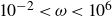 $10^{-2}\lt \omega \lt 10^{6}$
;
$10^{-2}\lt \omega \lt 10^{6}$
;
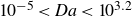 $10^{-5}\lt {\textit{Da}}\lt 10^{3.2}$
;
$10^{-5}\lt {\textit{Da}}\lt 10^{3.2}$
;
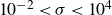 $10^{-2}\lt \sigma \lt 10^{4}$
;
$10^{-2}\lt \sigma \lt 10^{4}$
;
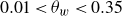 $0.01\lt \theta _w\lt 0.35$
, each probing 10 values in the respective range. Every possible combination is tested resulting in
$0.01\lt \theta _w\lt 0.35$
, each probing 10 values in the respective range. Every possible combination is tested resulting in
 $10^4 = 10\,000$
unique transient simulations. The remaining salient parameters are
$10^4 = 10\,000$
unique transient simulations. The remaining salient parameters are
 $\Delta z_\infty = 0.1$
,
$\Delta z_\infty = 0.1$
,
 $\theta _D = 10$
,
$\theta _D = 10$
,
 $\xi = -1.5$
,
$\xi = -1.5$
,
 ${\textit{Sc}} = 0.5$
,
${\textit{Sc}} = 0.5$
,
 ${\textit{Pr}} = 0.71$
,
${\textit{Pr}} = 0.71$
,
 $\alpha _e = 0.6$
,
$\alpha _e = 0.6$
,
 $\beta = 7500\,\textrm {s}^{-1}$
,
$\beta = 7500\,\textrm {s}^{-1}$
,
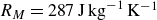 $R_M=287\,\textrm {J}\,\textrm {kg}^{-1}\,\textrm {K}^{-1}$
,
$R_M=287\,\textrm {J}\,\textrm {kg}^{-1}\,\textrm {K}^{-1}$
,
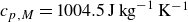 $c_{p,M}=1004.5\,\textrm {J}\,\textrm {kg}^{-1}\,\textrm {K}^{-1}$
.
$c_{p,M}=1004.5\,\textrm {J}\,\textrm {kg}^{-1}\,\textrm {K}^{-1}$
.
The correlation in (2.40) reveals that the problem is mostly dependent on four non-dimensional parameters: the three length-scale ratios
 $\delta _c/l_w$
,
$\delta _c/l_w$
,
 $\delta _S/l_w$
,
$\delta _S/l_w$
,
 $\delta _c/\delta _S$
and the Damkoehler number
$\delta _c/\delta _S$
and the Damkoehler number
 $Da$
. For this reason, the results obtained from the numerical simulation are plotted against these four scaling parameters. The results are shown in figure 9, where the % difference between numerical solution and correlation (2.40) is presented. All four figures present the same dataset, and it can be seen that the largest deviation amounts to
$Da$
. For this reason, the results obtained from the numerical simulation are plotted against these four scaling parameters. The results are shown in figure 9, where the % difference between numerical solution and correlation (2.40) is presented. All four figures present the same dataset, and it can be seen that the largest deviation amounts to
 $-12.5$
% and
$-12.5$
% and
 $9$
%. Given the approximate engineering approach taken, this level of agreement is adequate. The agreement is especially good at high frequencies (small Stokes-layer thickness
$9$
%. Given the approximate engineering approach taken, this level of agreement is adequate. The agreement is especially good at high frequencies (small Stokes-layer thickness
 $\delta _S$
), large Damkoehler numbers and highly catalytic surface conditions. Each of these effects reduces the magnitude of wall fluctuations to very small values, which is accurately captured by the correlation. The good agreement between simulation and correlation is due to the fact that diffusion processes very quickly limit the penetration depth, i.e. the Stokes-layer thickness, such that the oscillation amplitude is attenuated already close to the boundary-layer edge. This then effectively reduces the boundary-layer-edge perturbation magnitude for a quasi-equilibrium case. This behaviour motivated the use of a simple multiplication of diffusion and chemical attenuation terms, as employed in § 2.4.
$\delta _S$
), large Damkoehler numbers and highly catalytic surface conditions. Each of these effects reduces the magnitude of wall fluctuations to very small values, which is accurately captured by the correlation. The good agreement between simulation and correlation is due to the fact that diffusion processes very quickly limit the penetration depth, i.e. the Stokes-layer thickness, such that the oscillation amplitude is attenuated already close to the boundary-layer edge. This then effectively reduces the boundary-layer-edge perturbation magnitude for a quasi-equilibrium case. This behaviour motivated the use of a simple multiplication of diffusion and chemical attenuation terms, as employed in § 2.4.
4. Discussion
This section provides further analysis of the properties of unsteady mass diffusion in a non-equilibrium boundary layer. In particular, the implications for the diffusive heat flux and a non-dimensional representation of the salient scaling parameters are given. Figure 10 highlights the behaviour of some special cases. In the case of frozen flow (small Damkoehler number), the solution is entirely diffusion controlled and correlation (2.15) provides an adequate description of the problem. If, furthermore, the oscillation frequency is low, correlations (2.15) (only considers diffusion) and (2.35) (only considers quasi-steady solutions) converge to the same point. In general, even for the equilibrium case (
 ${\textit{Da}} = 1.6\times 10^3$
) shown in figure 10, the wall concentration magnitude will always tend towards the quasi-steady limit. For low frequencies, the propagation speed of concentration changes is fast enough to result in quasi-steady conditions. In the investigated parameter space, this tends to be the case for frequencies lower than
${\textit{Da}} = 1.6\times 10^3$
) shown in figure 10, the wall concentration magnitude will always tend towards the quasi-steady limit. For low frequencies, the propagation speed of concentration changes is fast enough to result in quasi-steady conditions. In the investigated parameter space, this tends to be the case for frequencies lower than
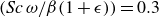 $({{\textit{Sc}} \, \omega }/{ \beta (1+\epsilon ) }) = 0.3$
. This means that the quasi-steady solution will always set the maximum possible wall-fluctuation magnitude. Similarly, this means that a quasi-steady limit can never exceed the limit set by the diffusion processes, as is evident for the frozen (
$({{\textit{Sc}} \, \omega }/{ \beta (1+\epsilon ) }) = 0.3$
. This means that the quasi-steady solution will always set the maximum possible wall-fluctuation magnitude. Similarly, this means that a quasi-steady limit can never exceed the limit set by the diffusion processes, as is evident for the frozen (
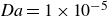 ${\textit{Da}} = 1\times 10^{-5}$
) case shown in figure 10.
${\textit{Da}} = 1\times 10^{-5}$
) case shown in figure 10.
Comparison between simulations and analytical correlations considering either diffusion or quasi-steady reaction domination, and their combination for cases of nearly frozen and nearly equilibrium flow. Numerical simulation results are given by individual symbols, while correlations are given by lines.

Values of
 $\Delta z_w / \Delta z_\infty$
for different Damkoehler numbers. (a)
$\Delta z_w / \Delta z_\infty$
for different Damkoehler numbers. (a)
 $Da = 1 \times 10^{-5}$
which is nearly frozen,(b)
$Da = 1 \times 10^{-5}$
which is nearly frozen,(b)
 $Da = 0.35$
and (c)
$Da = 0.35$
and (c)
 $Da = 1 \times 10^{-5}$
which is nearly equilibrium.
$Da = 1 \times 10^{-5}$
which is nearly equilibrium.
 $Da = 1584$
which is nearly equilibrium.
$Da = 1584$
which is nearly equilibrium.

Figure 11 shows an overview of the wall concentration fluctuation magnitude. Three Damkoehler numbers are presented corresponding to a nearly frozen regime, an intermediate regime and a nearly equilibrium regime. The magnitude of wall fluctuation reduces significantly as the Damkoehler number is increased. Furthermore, the magnitude is reduced for high frequencies and high catalytic factors
 $\sigma$
. As the Damkoehler number increases, the area with relatively larger fluctuations extends toward higher values of
$\sigma$
. As the Damkoehler number increases, the area with relatively larger fluctuations extends toward higher values of
 $\sigma$
. These figures can be significant for understanding the presence of atoms near the surface if gas–surface interaction is observed. Clearly, high catalycity and equilibrium flow suppress the influence of external fluctuations almost completely. Hence, test cases featuring these characteristics may be less affected by unsteady free-stream conditions. If materials are reaction-limited as opposed to diffusion-limited, larger atomic-mass-fraction fluctuations can occur at the surface. These conditions may lead to an underestimation of atomic partial pressures and therefore uncertainties in the determination of gas–surface interaction parameters, such as catalycity.
$\sigma$
. These figures can be significant for understanding the presence of atoms near the surface if gas–surface interaction is observed. Clearly, high catalycity and equilibrium flow suppress the influence of external fluctuations almost completely. Hence, test cases featuring these characteristics may be less affected by unsteady free-stream conditions. If materials are reaction-limited as opposed to diffusion-limited, larger atomic-mass-fraction fluctuations can occur at the surface. These conditions may lead to an underestimation of atomic partial pressures and therefore uncertainties in the determination of gas–surface interaction parameters, such as catalycity.
The current work utilises self-similar boundary-layer theory, which implies thermochemical equilibrium at the boundary-layer edge (Goulard (Reference Goulard1958)). Therefore, fluctuations in atomic mass fraction are necessarily accompanied by fluctuations in temperature. The coupling between these two effects is not included in (2.40). The error introduced through this omission is largest when small fluctuation frequencies are present, as the temperature field needs to penetrate deep into the boundary layer to affect the reaction term (2.6) enough to significantly alter the wall atomic mass fraction. An assessment of the temperature penetration depth can be carried out using Hermann (Reference Hermann2025).
4.1. Diffusive heat flux
The diffusive heat flux due to heterogeneous catalytic recombination at the wall can be calculated as
 \begin{equation} \dot {q}_{w,D} = - \frac {\sqrt { \beta C \rho _e \mu _e (1+\epsilon ) } c_{p,M} T_e H_D }{\sqrt {2} \, {\textit{Pr}} } z'(0) \end{equation}
with
 \begin{equation} z'(0) = \sigma z(0), \end{equation}
due to the boundary condition at the wall (Inger (Reference Inger1963)). This formulation assumes a full energy accommodation of the exothermic recombination reaction. In the nominal case without external fluctuations, the wall concentration shall be
 $z_n$
. In the case of fluctuations with amplitude
$z_n$
. In the case of fluctuations with amplitude
 $\Delta z_\infty$
, the wall concentration is oscillating with between
$\Delta z_\infty$
, the wall concentration is oscillating with between
 $z^\Delta = z_n \pm \Delta z_w$
. Utilising (2.40) and (2.35), this is simplified to
$z^\Delta = z_n \pm \Delta z_w$
. Utilising (2.40) and (2.35), this is simplified to
 \begin{equation} z^\Delta = z_n \left ( 1 \pm \Delta z_\infty \left [A \left ( \delta _{T,L} \right ) - \frac { A\left ( \delta _{T,L} \right ) - A\left ( \delta _{T,T} \right ) }{ 1 + 8.2 \left ( \frac {{\textit{Sc}} \, \omega }{ \beta (1+\epsilon ) } \right )^{-3} } \right ] \right ). \end{equation}
Calculating the ratio between diffusive wall heat fluxes for both the steady-state
 $\dot {q}_{w,D}$
and the fluctuating case
$\dot {q}_{w,D}$
and the fluctuating case
 $\dot {q}^\Delta _{w,D}$
reveals that the nominal wall concentration
$\dot {q}^\Delta _{w,D}$
reveals that the nominal wall concentration
 $z_n$
cancels out completely, and the problem becomes controlled entirely by the diffusive nature of the boundary layer,
$z_n$
cancels out completely, and the problem becomes controlled entirely by the diffusive nature of the boundary layer,
 \begin{equation} \frac {\dot {q}^\Delta _{w,D}}{\dot {q}_{w,D}} = 1 \pm \Delta z_\infty \left [A \left ( \delta _{T,L} \right ) - \frac { A\left ( \delta _{T,L} \right ) - A\left ( \delta _{T,T} \right ) }{ 1 + 8.2 \left ( \frac {{\textit{Sc}} \, \omega }{ \beta (1+\epsilon ) } \right )^{-3} } \right ]. \end{equation}
Equation (4.4) is evaluated for the dataset described in § 3.3 and the difference between numerical simulation and correlation is presented in figure 12. A maximum deviation of 6 % and
 $-3$
% is observed, showing a good accuracy of this correlation. This corroborates the finding that the diffusive inertia of the boundary layer is the only significant physical mechanism when the diffusive heat flux is considered. This interesting result highlights that no knowledge of the absolute wall concentration is necessary. This means that the change of diffusive heat flux due to external fluctuations is insensitive to the rate of chemical reactions taking place in the boundary layer, i.e. it is no function of the Damkoehler number. Furthermore, this ratio is also only a weak function of surface catalycity. Figure 13 substantiates this finding and shows the relative augmentation of diffusive heat flux. Here,
$-3$
% is observed, showing a good accuracy of this correlation. This corroborates the finding that the diffusive inertia of the boundary layer is the only significant physical mechanism when the diffusive heat flux is considered. This interesting result highlights that no knowledge of the absolute wall concentration is necessary. This means that the change of diffusive heat flux due to external fluctuations is insensitive to the rate of chemical reactions taking place in the boundary layer, i.e. it is no function of the Damkoehler number. Furthermore, this ratio is also only a weak function of surface catalycity. Figure 13 substantiates this finding and shows the relative augmentation of diffusive heat flux. Here,
 $\Delta \dot {q}_{w,D} / \Delta z_\infty$
represents
$\Delta \dot {q}_{w,D} / \Delta z_\infty$
represents
 $ ( ({\dot {q}^\Delta _{w,D}}/{\dot {q}_{w,D}}) - 1 ) / \Delta z_\infty$
. This value can be interpreted as the diffusive heat flux amplitude per external atomic concentration amplitude. It can be seen that for slow fluctuations, the diffusive heat flux augmentation is no function of catalycity. In an intermediate regime near
$ ( ({\dot {q}^\Delta _{w,D}}/{\dot {q}_{w,D}}) - 1 ) / \Delta z_\infty$
. This value can be interpreted as the diffusive heat flux amplitude per external atomic concentration amplitude. It can be seen that for slow fluctuations, the diffusive heat flux augmentation is no function of catalycity. In an intermediate regime near
 $({{\textit{Sc}} \, \omega }/{ \beta (1+\epsilon ) }) = 1$
, catalycity affects the diffusive heat flux. For fast fluctuations, the diffusive heat flux is completely dampened and external flow variations are irrelevant.
$({{\textit{Sc}} \, \omega }/{ \beta (1+\epsilon ) }) = 1$
, catalycity affects the diffusive heat flux. For fast fluctuations, the diffusive heat flux is completely dampened and external flow variations are irrelevant.
Comparison between diffusive heat flux amplitudes derived through numerical simulation and (4.4).

Diffusive heat flux fluctuation amplitude per free-stream atom mass fraction fluctuation amplitude.

4.2. Non-dimensional heat and mass-transfer form
This section utilises non-dimensional parameters to generalise the findings on unsteady species transport. The derivation in § 2.2 resulted in the identification of three length-scale ratios that completely define the behaviour of the diffusion-limited case, these are
 $({\delta _c}/{\delta _S})$
,
$({\delta _c}/{\delta _S})$
,
 $({\delta _c}/{l_w})$
and
$({\delta _c}/{l_w})$
and
 $({\delta _S}/{l_w})$
(see figure 2). In the following, these ratios will be expressed using non-dimensional heat and mass-transfer numbers. The following simplifications are employed: a unity Chapman–Rubesin factor
$({\delta _S}/{l_w})$
(see figure 2). In the following, these ratios will be expressed using non-dimensional heat and mass-transfer numbers. The following simplifications are employed: a unity Chapman–Rubesin factor
 $C = \rho \mu / (\rho _e \mu _e) = 1$
and an incompressible boundary layer. This simplifies the coordinate transformation (2.3) into
$C = \rho \mu / (\rho _e \mu _e) = 1$
and an incompressible boundary layer. This simplifies the coordinate transformation (2.3) into
 \begin{equation} \eta _c = \sqrt {\frac {(1+\epsilon ) \beta }{\nu _e}} y. \end{equation}
where
 $\nu_e$
is the boundary layer edge kinematic viscosity. Using the definition of the Nusselt number,
$\nu_e$
is the boundary layer edge kinematic viscosity. Using the definition of the Nusselt number,
 \begin{equation} {Nu} = \frac {h D_\eta }{k}, \end{equation}
with characteristic diameter
 $D_\eta$
, which is
$D_\eta$
, which is
 \begin{equation} D_\eta = \sqrt {\frac {(1+\epsilon ) \beta }{\nu _e}} D, \end{equation}
where
 $D$
is the real diameter of the sphere and
$D$
is the real diameter of the sphere and
 $D_\eta$
is that same diameter transformed by (4.5). The heat transfer coefficient in transformed
$D_\eta$
is that same diameter transformed by (4.5). The heat transfer coefficient in transformed
 $\eta$
coordinates is calculated via
$\eta$
coordinates is calculated via
 \begin{equation} h = \frac {\dot {q}^\eta _w}{1 - \theta _w}, \end{equation}
where
 \begin{equation} \dot {q}^\eta _w = - k \frac {\partial \theta }{\partial \eta }. \end{equation}
where
 $k$
is the thermal conductivity. Combining this with (2.18) or (2.19) gives the thermal boundary-layer thickness in non-dimensional transformed variables (
$k$
is the thermal conductivity. Combining this with (2.18) or (2.19) gives the thermal boundary-layer thickness in non-dimensional transformed variables (
 $\eta$
-space),
$\eta$
-space),
 \begin{equation} \delta _{T,L} = \sqrt {\frac {(1+\epsilon ) \beta }{\nu _e}} \frac {D}{{Nu}}, \,\,\,\,\,\\ \delta _{T,T} = 2 \sqrt {\frac {(1+\epsilon ) \beta }{\nu _e}} \frac {D}{{Nu}}, \end{equation}
yielding the respective concentration boundary-layer thickness with (2.20)
 \begin{equation} \delta _c = \sqrt {\frac {(1+\epsilon ) \beta }{\nu _e}} \frac {D}{{Nu} \sqrt {{Le}}}, \,\,\,\,\,\, \mathrm{or} \,\,\,\,\,\, \delta _c = 2 \sqrt {\frac {(1+\epsilon ) \beta }{\nu _e}} \frac {D}{{Nu} \sqrt {{Le}}}. \end{equation}
The Stokes-layer thickness defined in (2.16) can be transformed into
 \begin{equation} \delta _S = D \sqrt {\frac {(1+\epsilon ) \beta }{\nu _e}} \sqrt {\frac {2}{{Re} \, {\textit{Sc}} \, {Sr} }} \end{equation}
with Strouhal and Reynolds numbers
 \begin{equation} {Sr} = \frac {\omega D}{U_\infty }; \,\,\,\,\mathrm{and}\,\,\,\, {Re} = \frac {U_\infty D}{\nu }. \end{equation}
where
 $U_\infty$
is the flow velocity. The ratio of these two length scales is then found by combining (4.11) and (4.12) into
$U_\infty$
is the flow velocity. The ratio of these two length scales is then found by combining (4.11) and (4.12) into
 \begin{equation} \frac {\delta _c}{\delta _S} = \frac {1}{\sqrt {2}} \frac {\sqrt { {Re} \, {\textit{Pr}} \, {Sr} }}{{Nu}}, \,\,\,\,\,\, \mathrm{or} \,\,\,\,\,\, \frac {\delta _c}{\delta _S} = \sqrt {2} \frac {\sqrt { {Re} \, {\textit{Pr}} \, {Sr} }}{{Nu}}, \end{equation}
where the first version is based on
 $\delta _T = \delta _{T,L}$
, and the second is based on
$\delta _T = \delta _{T,L}$
, and the second is based on
 $\delta _T = \delta _{T,T}$
. Curiously, this result is identical for the analogous case of heat transfer oscillations (Hermann Reference Hermann2025). This case considers the propagation of unsteady temperature fluctuations through the boundary layer, and it was found that the ratio of thermal-boundary-layer thickness to Stokes-layer thickness is given by (4.14). It would be expected that for the case considered in this work, i.e. the equivalent mass-transfer problem, Prandtl and Schmidt numbers should be exchanged. However, the Schmidt-number dependence is entirely cancelled out due to the connection of the thermal and concentration boundary layers via the Lewis number scaling in (2.20).
$\delta _T = \delta _{T,T}$
. Curiously, this result is identical for the analogous case of heat transfer oscillations (Hermann Reference Hermann2025). This case considers the propagation of unsteady temperature fluctuations through the boundary layer, and it was found that the ratio of thermal-boundary-layer thickness to Stokes-layer thickness is given by (4.14). It would be expected that for the case considered in this work, i.e. the equivalent mass-transfer problem, Prandtl and Schmidt numbers should be exchanged. However, the Schmidt-number dependence is entirely cancelled out due to the connection of the thermal and concentration boundary layers via the Lewis number scaling in (2.20).
The ratio between Stokes-layer thickness and surface catalycity length scale
 $ ({\delta _S}/{l_w})$
can be further simplified as well, using the definition of the catalycity factor
$ ({\delta _S}/{l_w})$
can be further simplified as well, using the definition of the catalycity factor
 $\sigma$
in (2.11). Introducing the assumptions of a unity Chapman–Rubesin factor, and an equivalence of wall and boundary-layer-edge viscosity, the surface catalytic factor can be simplified to
$\sigma$
in (2.11). Introducing the assumptions of a unity Chapman–Rubesin factor, and an equivalence of wall and boundary-layer-edge viscosity, the surface catalytic factor can be simplified to
 \begin{equation} \sigma = \frac {1}{l_w} \approx {\textit{Sc}} \, K_w \sqrt { \frac {2}{(1+\epsilon ) \beta \nu } }. \end{equation}
where
 $\nu$
is the kinematic viscosity. Using the definition of the Stokes-layer depth from (2.16), the length-scale ratio becomes
$\nu$
is the kinematic viscosity. Using the definition of the Stokes-layer depth from (2.16), the length-scale ratio becomes
 \begin{equation} \frac {\delta _S}{l_w} = 2 \gamma \sqrt {\frac {{\textit{Sc}}\, R_m T_w }{\pi \omega \nu }}. \end{equation}
This can be further simplified into
 \begin{equation} \frac {\delta _S}{l_w} = \frac {2 \gamma }{\sqrt {\pi }} \sqrt {\frac {{\textit{Sc}}\,{Re} }{ {Sr} }} \sqrt {\frac {R_m T_w}{U_\infty ^2}}. \end{equation}
The last term in this formulation,
 $\sqrt {({R_m T_w}/{U_\infty ^2})}$
, can be interpreted as a ratio of internal energy at wall conditions to bulk kinetic energy. Finally, the ratio between boundary-layer thickness and catalycity length scale
$\sqrt {({R_m T_w}/{U_\infty ^2})}$
, can be interpreted as a ratio of internal energy at wall conditions to bulk kinetic energy. Finally, the ratio between boundary-layer thickness and catalycity length scale
 $ ({\delta _c}/{l_w})$
can be further simplified using (4.15) and (4.11) into
$ ({\delta _c}/{l_w})$
can be further simplified using (4.15) and (4.11) into
 \begin{equation} \frac {\delta _c}{l_w} = \gamma \sqrt {\frac {2}{\pi }} \frac { {Re} \sqrt { {\textit{Sc}}\, {\textit{Pr}} }}{ {Nu} } \sqrt {\frac {R_m T_w}{U_\infty ^2}}, \,\,\,\,\,\, \mathrm{or} \,\,\,\,\,\, \frac {\delta _c}{l_w} = 2 \gamma \sqrt {\frac {2}{\pi }} \frac { {Re} \sqrt { {\textit{Sc}}\, {\textit{Pr}} }}{ {Nu} } \sqrt {\frac {R_m T_w}{U_\infty ^2}}. \end{equation}
5. Experimental case study
In this section the derived theory is applied to an experimental case study based on the works of Marynowski et al. (Reference Marynowski, Loehle, Fasoulas, Meindl and Zander2014) and Zander et al. (Reference Zander, Marynowski and Löhle2017). The experiments were carried out in the University of Stuttgart’s PWK3 inductively coupled plasma wind tunnel, with operating conditions summarised in table 1. The CO
 $_2$
plasma free-jet is used as a case study to investigate how real flow conditions are affected by unsteady species transport. The analysis carried out is not a detailed replication of the experiment, but rather uses realistic experimental operating conditions to investigate the order of magnitude of fluctuations in atomic mass fraction and diffusive heat flux. To this end, several simplifications are made for the purpose of calculating edge conditions for the boundary layer: equilibrium flow is assumed fluctuating between 2800 K and 6000 K (Zander et al. (Reference Zander, Marynowski and Löhle2017)) yielding a mean atomic oxygen mass fraction of
$_2$
plasma free-jet is used as a case study to investigate how real flow conditions are affected by unsteady species transport. The analysis carried out is not a detailed replication of the experiment, but rather uses realistic experimental operating conditions to investigate the order of magnitude of fluctuations in atomic mass fraction and diffusive heat flux. To this end, several simplifications are made for the purpose of calculating edge conditions for the boundary layer: equilibrium flow is assumed fluctuating between 2800 K and 6000 K (Zander et al. (Reference Zander, Marynowski and Löhle2017)) yielding a mean atomic oxygen mass fraction of
 $\alpha _e = 0.672$
with a fluctuation intensity of
$\alpha _e = 0.672$
with a fluctuation intensity of
 $\Delta c_\infty = 0.2695$
. These values have been computed using NASA’s Chemical Equilibrium and Applications program (McBride & Gordon Reference McBride and Gordon1996). Only the reaction
$\Delta c_\infty = 0.2695$
. These values have been computed using NASA’s Chemical Equilibrium and Applications program (McBride & Gordon Reference McBride and Gordon1996). Only the reaction
 $ \mathrm{CO} \rightarrow \mathrm{C} + \mathrm{O}$
is considered, as this mechanisms dominates in the investigated temperature range, and since additional reactions are beyond the scope of the developed model. Furthermore, constant thermophysical and transport properties are assumed. The wall heat flux consists of a conductive and a diffusive component (Inger (Reference Inger1963)), which are combined to yield the total wall heat flux:
$ \mathrm{CO} \rightarrow \mathrm{C} + \mathrm{O}$
is considered, as this mechanisms dominates in the investigated temperature range, and since additional reactions are beyond the scope of the developed model. Furthermore, constant thermophysical and transport properties are assumed. The wall heat flux consists of a conductive and a diffusive component (Inger (Reference Inger1963)), which are combined to yield the total wall heat flux:
 \begin{equation} \dot {q}_w =- \frac { \sqrt { (1+\epsilon )/2 \,\,\, \beta C \rho _e \mu _e }}{{\textit{Pr}} / (C_{p,m} T_e)} \left ( \theta '(0) + H_D z'(0) \right ). \end{equation}
In this analysis, only the unsteady behaviour of the diffusive component is considered to isolate the contribution of atomic recombination only. In a real flow, additional unsteadiness in other flow variables, e.g. temperature, velocity, density, may be present. However, this is beyond the scope of the current analysis, which is aimed at understanding the contribution of atomic recombination only.
Experimental test conditions extracted from Marynowski et al. (Reference Marynowski, Loehle, Fasoulas, Meindl and Zander2014) and Zander et al. (Reference Zander, Marynowski and Löhle2017).

Fluctuation magnitude of wall atomic mass fraction
 $\alpha$
.
$\alpha$
.
 $C_{A,wall}$
is the atomic mass fraction at the wall.
$C_{A,wall}$
is the atomic mass fraction at the wall.

The absolute atomic oxygen wall mass fraction
 $c_A$
is presented in figure 14 for a range of Damkoehler numbers and wall catalycities. As is expected from the discussion in § 4, the largest variation occurs for a non-catalytic material under frozen conditions, reaching a maximum oscillation amplitude of 18 %. Higher catalycities and larger Damkoehler numbers significantly reduce the oscillation magnitude. Figure 15 shows the influence of unsteady atomic mass transport on the diffusive heat flux. The ratio of the diffusive heat flux amplitude over the total average heat flux is shown. The highest fluctuation occurs for highly catalytic surfaces, as most incoming atoms are recombined to molecules, releasing their exothermic recombination energy into the material surface. The largest fluctuation amplitude occurs for nearly frozen flow, while larger Damkoehler numbers slightly reduce the magnitude of the fluctuation. In the investigated case, the heat flux can vary by as much as 22 % for a fully catalytic surface, showing the severe influence of unsteady species transport. Even though this variation magnitude is significant, the influence of the heat flux variation on a sample wall temperature is likely very small due to the low density of this flow condition. A detailed discussion of this phenomenon is given in Hermann (Reference Hermann2025).
$c_A$
is presented in figure 14 for a range of Damkoehler numbers and wall catalycities. As is expected from the discussion in § 4, the largest variation occurs for a non-catalytic material under frozen conditions, reaching a maximum oscillation amplitude of 18 %. Higher catalycities and larger Damkoehler numbers significantly reduce the oscillation magnitude. Figure 15 shows the influence of unsteady atomic mass transport on the diffusive heat flux. The ratio of the diffusive heat flux amplitude over the total average heat flux is shown. The highest fluctuation occurs for highly catalytic surfaces, as most incoming atoms are recombined to molecules, releasing their exothermic recombination energy into the material surface. The largest fluctuation amplitude occurs for nearly frozen flow, while larger Damkoehler numbers slightly reduce the magnitude of the fluctuation. In the investigated case, the heat flux can vary by as much as 22 % for a fully catalytic surface, showing the severe influence of unsteady species transport. Even though this variation magnitude is significant, the influence of the heat flux variation on a sample wall temperature is likely very small due to the low density of this flow condition. A detailed discussion of this phenomenon is given in Hermann (Reference Hermann2025).
Relative magnitude of fluctuating wall heat flux.
 $\Delta_{q^{\omega}}$
is the diffusive heat flux amplitude and
$\Delta_{q^{\omega}}$
is the diffusive heat flux amplitude and
 $q_{total}$
is the total time-averaged heat flux
$q_{total}$
is the total time-averaged heat flux

A real non-equilibrium multi-species flow may exhibit additional effects not captured in the current analysis, e.g. additional chemical reactions, thermal non-equilibrium, temperature-dependent transport properties. However, the investigation carried out here provides insight into regions of high fluctuation intensity and gives an approximate account of expected magnitudes. Furthermore, the study motivates a more detailed numerical investigation of unsteady flows in ground testing facilities, a trend currently in development in the literature; see e.g. in Sirmalla et al. (Reference Sirmalla, Munafò, Kumar, Bodony and Panesi2024). The significant magnitudes of heat flux and atomic-mass-fraction fluctuation derived from the current work give rise to uncertainties in the interpretation of test data in highly unsteady flows. Amongst other sources of uncertainty, this is likely a contributing factor to why experimentally derived recombination coefficients vary by orders of magnitude in the literature (Kim et al. Reference Kim, Yang, Park and Jo2021b ; Massuti-Ballester & Herdrich Reference Massuti-Ballester and Herdrich2021; Chazot et al. Reference Chazot, Panerai, Muylaert and Thoemel2010). As detailed heterogeneous catalytic recombination mechanisms can depend on the atomic partial pressure at the surface, a large fluctuation amplitude could lead to significant uncertainty in the experimental determination of catalytic recombination coefficients. Accurate experimental interpretation will require a detailed assessment of the unsteady nature of the flow and its effect on the surface conditions. Besides the interpretation of material tests, these effects may also affect basic facility calibration methods, as many enthalpy probes rely on cold-wall heat flux measurements to highly catalytic surfaces (Valeinis, Chang & Hermann Reference Valeinis, Chang and Hermann2024).
6. Conclusion
A correlation modelling unsteady atomic mass transport in a non-equilibrium boundary layer has been established. Exact analytical solutions to diffusion- and reaction-dominated formulations of the boundary-layer equations are used alongside empirical correlations. The theory assumes constant thermophysical properties, in a self-similar stagnation-point boundary layer, where a generic Lighthill gas undergoes dissociation and recombination reactions. The derived theory considers single frequency fluctuations, but allows their superposition due to the linear time-invariant property of the correlation. The generalised theory describes the unsteady non-equilibrium mass transport of atomic species, and is shown to be dependent only on the steady-state frozen solutions of the boundary layer. The accuracy of the semi-empirical approach has been assessed by comparing it with fully transient simulations of the coupled boundary-layer equations. Simulated wall-fluctuation magnitudes of atomic mass fraction agree with the correlation to within 12.5 %.
The analytical approach taken in this work leads to the identification of the salient scaling parameters of unsteady mass transport. Alongside the Damkoehler number, these can be interpreted as length-scale ratios of Stokes-layer thickness, concentration boundary-layer thickness and wall catalytic length scale. It is shown that the highest wall-fluctuation magnitudes occur for frozen conditions and non-catalytic or severely reaction-limited wall conditions. Instead, large Damkoehler numbers and high wall catalycity significantly attenuate the fluctuation intensity. The fluctuation of diffusive heat flux is found to be independent of Damkoehler number and entirely described by the diffusive transport properties of the boundary layer.
The derived theory aids in the analysis of experiments investigating the gas surface interaction of high-temperature materials subjected to high-enthalpy flow conditions. Historically, these experiments have been assessed using steady-state assumptions. Wall conditions have a significant influence on the determination of gas–surface interaction rates. The current work shows that under realistic operating conditions of high-enthalpy facilities, significant fluctuations of atomic wall concentration and diffusive heat flux can be expected, introducing uncertainty in the commonly used interpretation of experimental data. Furthermore, cold-wall probes used for facility calibration can be affected, introducing uncertainty in the determination of free-stream flow conditions.
The derived theory provides a first simple analytical framework, enabling improved analysis of transient high-enthalpy experiments. Furthermore, it motivates future studies employing higher-fidelity models in order to remove uncertainty in the determination of gas–surface interaction rates.
Funding
This research was funded by the UKRI Future Leaders Fellowship scheme (grant number MR/T041269/1), and we extend our gratitude to UKRI. For Open Access, the author has applied for a CC BY public copyright license to any Author Accepted Manuscript (AAM) version arising from this submission.
Declaration of interests
The author reports no conflict of interest.


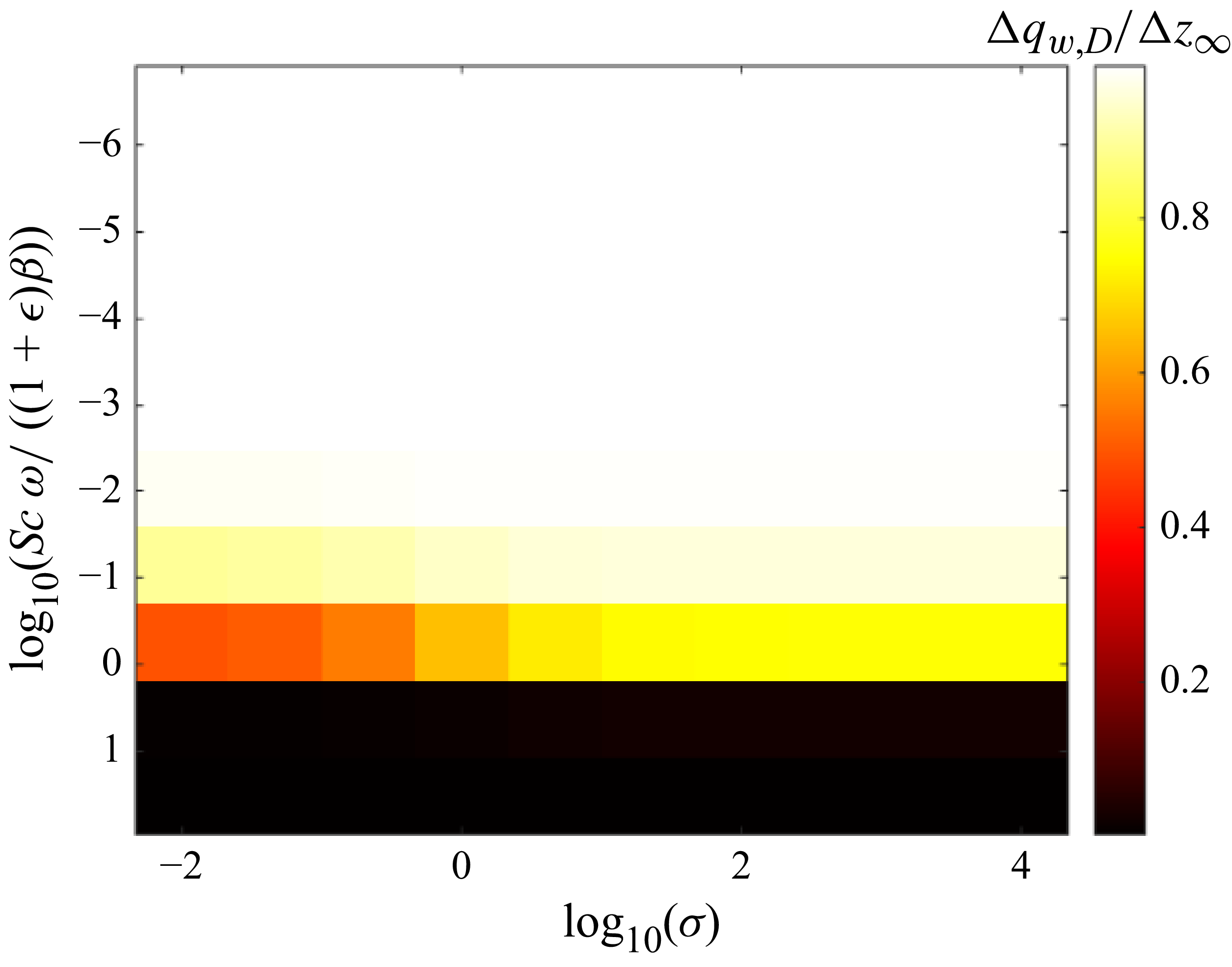
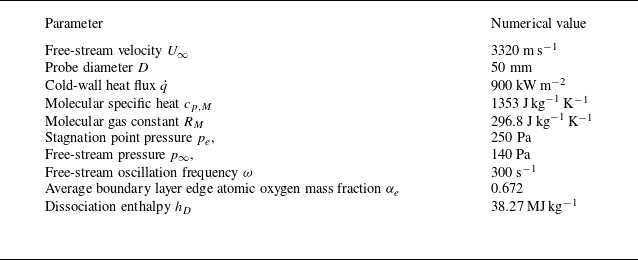


 Open access