2.1. Model equations

The electrons are described by a four-component distribution function $(f_0, {\boldsymbol f})(t, {x}, {v})$ with ${\boldsymbol f} = (f_1, f_2, f_3)\in \mathbb {R}^3$, which is coupled to the continuous ion spin distribution ${\boldsymbol S}(t, x) = (S_1, S_2, S_3)(t, x)$. The overall system of equations, for the space variable $x\in [0, L]\subset \mathbb {R}$ and velocity variable $v\in \mathbb {R}$, is composed of a set of kinetic equations for the electron distribution functions (Manfredi et al. Reference Manfredi, Hervieux and Hurst2019; Crouseilles et al. Reference Crouseilles, Hervieux, Hong and Manfredi2023),

(2.1)\begin{gather} \frac{\partial f_0}{\partial t} + {v} \frac{\partial f_0}{\partial { x}} + \frac{e}{m} \frac{\partial V_H}{\partial { x}} \frac{\partial f_0}{\partial { v}} - \frac{\mu_B }{m} \frac{\partial {\boldsymbol B}}{\partial x}\boldsymbol{\cdot} \frac{\partial {\boldsymbol f}}{\partial v}= 0, \end{gather}

(2.2)\begin{gather}\frac{\partial f_\ell}{\partial t} + {v} \frac{\partial f_\ell}{\partial { x}}+\frac{e}{m} \frac{\partial V_H}{\partial { x}} \frac{\partial f_\ell}{\partial { v}}- \frac{\mu_B }{m} \frac{\partial B_\ell}{\partial{ x}} \frac{\partial f_0}{\partial {v}} - \frac{e}{m}( {\boldsymbol B} \times {\boldsymbol f} )_\ell = 0, \quad \ell = 1, 2, 3, \end{gather}

and Landau–Lifshitz equation (Lakshmanan Reference Lakshmanan2011) for the ion spins,

(2.3)\begin{equation} \frac{\partial {\boldsymbol S}}{\partial t} = \frac{a^2 J }{\hbar}\left({\boldsymbol S} \times \frac{ \partial^2 {\boldsymbol S} }{\partial x^2} \right) + \frac{K}{2\hbar} {\boldsymbol S} \times \int {\boldsymbol f}\, \mathrm{d}{v}, \end{equation}

where the first term on the right-hand side is the Heisenberg ion–ion magnetic exchange, whereas the second term represents the ion–electron magnetic exchange.

The scalar distribution function $f_0(t,x,v)$ represents, as usual, the probability to find an electron in the phase space volume located around $(x,v)$, at time $t$. Its moments yield the usual macroscopic quantities, such as the density $n_e(t,x) = \int f_0(t, x, v) \, \mathrm {d} v$. In contrast, the vector distribution function $f_\ell (t,x,v)$ represents the mean spin polarization density of the electrons in the phase space volume located around $(x,v)$ at time $t$, along the $\ell$ direction. Its first moment ${\boldsymbol M}(t,x) = \int {\boldsymbol f}(t, x, v) \, \mathrm {d} v$ represents the electron spin density. For more details, see the recent review of Manfredi et al. (Reference Manfredi, Hervieux and Hurst2019). The relationship between this $(f_0, {\boldsymbol f})$ representation and the more standard representation as a $2 \times 2$ matrix with spin-up and spin-down components is also illustrated in Appendix A.

The self-consistent electric potential (Hartree potential) $V_H(t, x)$ obeys the Poisson equation

(2.4)\begin{equation} \varepsilon_0 \partial_x^2 V_H= e\int f_0 \,\mathrm{d}{v}- Ze\, n_{\rm ion}, \end{equation}

and the magnetic field appearing in (2.1) and (2.2) is primarily the one created by the ions

(2.5)\begin{equation} {\boldsymbol B}(t, x)={-}\frac{K n_{\rm ion} {\boldsymbol S (t, x)}}{2\mu_B}, \end{equation}

although external fields could also be considered. Here, $e>0$ denotes the electron charge, $\hbar$ the Planck constant, $m$ the electron mass, $\varepsilon _0$ the permittivity of vacuum, $\mu _B=e\hbar /2m$ the Bohr magneton, $a$ the interatomic distance, $Z$ is the atomic number, $J$ and $K$ are respectively the ion–ion and electron–ion magnetic exchange constants, and $n_{\rm ion}$ is the fixed, homogeneous ion density. The full initial condition may be denoted as $(f_0, {\boldsymbol f}, V_H, {\boldsymbol S})(t=0)=(f_0^{(0)}, {\boldsymbol f}^{(0)}, V_H^{(0)}, {\boldsymbol S}^{(0)})$, where $\varepsilon _0 \partial _x^2 V_H^{(0)}=e \int f_0^{(0)} \, \mathrm {d}{v}-Ze n_{\rm ion}$.

Note how the $K$-terms couple the ion and electron spin dynamics: the magnetic field ${\boldsymbol B}$ given by (2.5) created by the ions acts on the spin part of the electron distribution functions ${\boldsymbol f}$ in (2.1) and (2.2), while the electron spin density $\int {\boldsymbol f} \, \mathrm {d}{v}$ acts on the LL equation (2.3) for the ion spins. A schematic view of the physical system under consideration is shown in figure 1.

Figure 1.

Schematic view of the physical system under consideration. The immobile ions (red circles) provide the main source of localized magnetism. They interact through magnetic exchange both with themselves (coupling constant $J$) and with the itinerant electrons, represented by green dots (coupling constant $K$).

From a mathematical viewpoint, the model (2.1)–(2.4) enjoys a Poisson structure with the following Hamiltonian functional:

(2.6)\begin{align} \mathcal{H} = \frac{m}{2}\int {v}^2 f_0 \, \mathrm{d}\kern0.7pt {x} \, \mathrm{d}{v} + \mu_B \int {\boldsymbol f} \boldsymbol{\cdot} {\boldsymbol B} \, \mathrm{d}\kern0.7pt {x} \, \mathrm{d}{v} + \frac{\varepsilon_0}{2} \int (\partial_x V_H)^2 \, \mathrm{d}\kern0.7pt {x} + \frac{a^2 J }{2} \int n_{\rm ion} \sum_{\ell=1}^3 \left(\frac{\partial {S _\ell}}{\partial x}\right)^2 \, \mathrm{d}\kern0.7pt {x}. \end{align}

Moreover, it is possible to construct a Poisson bracket for two functionals $\mathcal {F}$ and $\mathcal {G}$ as

(2.7)\begin{align} \{\mathcal{F},\mathcal{G}\}& =\sum_{i=0}^3 \int \frac{f_0}{m} \left[ \frac{\delta \mathcal{F}}{\delta f_i}, \frac{\delta \mathcal{G}}{\delta f_i}\right]_{xv} \mathrm{d}\kern0.7pt {x}\,\mathrm{d}{v} \nonumber\\ & \quad + \sum_{i=1}^3 \left( \int \frac{f_i}{m} \left[ \frac{\delta \mathcal{F}}{\delta f_0}, \frac{\delta \mathcal{G}}{\delta f_i}\right]_{xv} \mathrm{d}\kern0.7pt {x}\,\mathrm{d}{v} + \int \frac{f_i}{m} \left[ \frac{\delta \mathcal{F}}{\delta f_i}, \frac{\delta \mathcal{G}}{\delta f_0}\right]_{xv} \mathrm{d}\kern0.7pt {x}\,\mathrm{d}{v} \right) \nonumber\\ & \quad +\frac{e}{\mu_B m} \int {\boldsymbol f} \boldsymbol{\cdot} \left( \frac{\delta \mathcal{F}}{\delta {\boldsymbol f}} \times \frac{\delta \mathcal{G}}{\delta {\boldsymbol f}}\right) \mathrm{d}\kern0.7pt {x}\,\mathrm{d}{v} + \frac{1}{\hbar}\int \frac{{\boldsymbol S} }{n_{\rm ion}} \boldsymbol{\cdot} \left( \frac{\delta \mathcal{F}}{\delta {\boldsymbol S} } \times \frac{\delta \mathcal{G}}{\delta {\boldsymbol S} }\right) \, \mathrm{d}\kern0.7pt {x}. \end{align}

With this notation in hand, the system (2.1)–(2.4) can be reformulated, after introducing the vector of unknowns $\mathcal {Z}=(f_0, {\boldsymbol f}, {\boldsymbol S} )\in \mathbb {R}^7$, as

(2.8)\begin{equation} \frac{\partial \mathcal{Z}}{\partial t} = \{ \mathcal{Z}, \mathcal{H} \}. \end{equation}

2.2. Normalized dimensionless equations

We rewrite the above (2.1)–(2.4) using dimensionless units that correspond to normalizing time to the inverse of the plasmon frequency $\omega _p=\sqrt {e^2n_e/\varepsilon _0 m}$, velocities to the thermal speed $v_{\rm th} = \sqrt {k_B T_e/m}$ and space to the Debye length $\lambda _D = v_{\rm th}/\omega _p$, where $k_B$ is the Boltzmann constant. Hence, the electric potential is normalized to $mv_{\rm th}^2/e$, the electric field to $mv_{\rm th}\omega _p/e$ and the magnetic field to $m \omega _p/e$.

Using these normalized units and defining the self-consistent electric field as $E_x=-\partial _x V_H$, the dimensionless kinetic equations read as (for simplicity of notation, we do not change the names of the dimensionless variables)

(2.9)\begin{gather} \frac{\partial f_0}{\partial t} + {v} \frac{\partial f_0}{\partial { x}} -E_x \frac{\partial f_0}{\partial { v}} - H \frac{\partial {\boldsymbol B}}{\partial{ x}}\boldsymbol{\cdot} \frac{\partial {\boldsymbol f}}{\partial { v}}= 0, \end{gather}

(2.10)\begin{gather}\frac{\partial f_\ell}{\partial t} + {v} \frac{\partial f_\ell}{\partial { x}}-E_x \frac{\partial f_\ell}{\partial { v}}- H \frac{\partial B_\ell}{\partial{ x}} \frac{\partial f_0}{\partial {v}} - ( {\boldsymbol B} \times {\boldsymbol f} )_\ell = 0, \quad \ell = 1, 2, 3, \end{gather}

where

(2.11)\begin{equation} {\boldsymbol B}={-}\frac{\tilde{K} {\boldsymbol S }}{2}\end{equation}

is the magnetic field created by the ions.

The dimensionless Planck constant,

(2.12)\begin{equation} H=\frac{\hbar \omega_p}{2 mv_{\rm th}^2}, \end{equation}

quantifies the relative importance of quantum effects with respect to thermal effects. We also note that $H$ can be written in terms of the quantum coupling parameter $\varGamma _q = \hbar \omega _p/E_F$ and the degeneracy parameter $\varTheta = T_e/T_F$ as $H = \varGamma _q/(2\varTheta )$. In turn, the quantum coupling parameter is related to the Wigner–Seitz radius $r_s$ through the following relationship (Bonitz et al. Reference Bonitz, Dornheim, Moldabekov, Zhang, Hamann, Kählert, Filinov, Ramakrishna and Vorberger2020):

(2.13)\begin{equation} \varGamma_q^2 = \frac{r_s}{a_0} \frac{16}{9{\rm \pi}} \left(\frac{12}{\rm \pi}\right)^{1/3} \approx 0.88 \frac{r_s}{a_0}, \end{equation}

where $a_0 = 4{\rm \pi} \varepsilon _0 \hbar ^2/(me^2)$ is the Bohr radius.

The normalized LL equation becomes

(2.14)\begin{equation} \frac{\partial {\boldsymbol S} }{\partial t} = A\left({\boldsymbol S} \times \frac{ \partial^2 {\boldsymbol S} }{\partial x^2} \right) + Z\frac{\tilde{K}}{4} {\boldsymbol S} \times \int {\boldsymbol f} \,\mathrm{d}{v}, \end{equation}

with the dimensionless magnetic exchange constants written as $A=({{a}^2}/{\lambda _D^2}) ({J}/{\hbar \omega _p})$ and $\tilde {K} = {2 K n_{\rm ion}}/{\hbar \omega _p}$. Finally, the dimensionless Poisson equation is

(2.15)\begin{equation} -\partial_x E_x=\int f_0 \, \mathrm{d}{v}-1. \end{equation}

The total energy in dimensionless units is given by the Hamiltonian $\mathcal {H}=\mathcal {H}_v+\mathcal {H}_E+ \sum _{i=1}^3(\mathcal {H}_{Z,i}+\mathcal {H}_{{\rm spin}, i})$, with

(2.16)\begin{equation} \left.\begin{array}{c@{}} \displaystyle \mathcal{H}_{v} = \dfrac{1}{2}\int v^2 f_0 \, \mathrm{d}\kern0.7pt {x}\,\mathrm{d}{v}, \quad \mathcal{H}_{E} = \dfrac{1}{2} \int \left(\dfrac{\partial V_H}{\partial x}\right)^2 \mathrm{d}\kern0.7pt {x},\\ \displaystyle \mathcal{H}_{Z,i} = H \int f_i B_i \, \mathrm{d}\kern0.7pt x\, \mathrm{d}v, \quad \mathcal{H}_{{\rm spin},i}= AH \int \left(\dfrac{\partial {S_i}}{\partial x}\right)^2 \mathrm{d}\kern0.7pt {x}, \end{array}\right\} \end{equation}

where the various terms correspond to the kinetic energy ($\mathcal {H}_{v}$), the Hartree electric energy ($\mathcal {H}_{E}$), the magnetic Zeeman energy ($\mathcal {H}_{Z}$) and the spin energy ($\mathcal {H}_\textrm {spin}$).

We consider an electron plasma in the WDM regime, with density $n_e = n_\textrm {ion} = 9.17 \times 10^{28} \ \textrm {m}^{-3}$ ($Z=1$) and temperature $k_B T_e = 16.58\ \textrm {eV}$. This choice yields for the time, velocity and length scales: $\omega _p=1.71\times 10^{16}\ \textrm {s}^{-1}$, $v_\textrm {th}=1.71 \times 10^6 \ \textrm {m s}^{-1}$ and $\lambda _D=10^{-10}\ \textrm {m}$. As for the dimensionless parameters, we find: normalized Planck constant $H=0.339$, quantum coupling parameter $\varGamma _q = 1.516$, Wigner–Seitz radius $r_s/a_0 = 2.60$ (corresponding to nickel) and degeneracy parameter $\varTheta = 2.24$.

For the magnetic exchange coupling constants, we use values close to those of nickel (Hurst et al. Reference Hurst, Hervieux and Manfredi2018): $J = 0.022\ \textrm {eV}$ and $K= 0.01 \ \textrm {eV} \ \textrm {nm}^3$. Taking the lattice spacing $a = 2 r_s = 0.275 \ \textrm {nm}$, this yields for the dimensionless parameters, $A=0.0148$ and $\tilde {K}=0.161$.

3.1. Linear analysis for a generic equilibrium

To validate the model (2.9)–(2.15) in the linear response regime, we perform a linear analysis to derive the pertinent dispersion relation. First, we start with the following homogeneous stationary state:

(3.1)\begin{equation} \left.\begin{array}{c@{}} f_0^{(0)}=f_0^{(0)}(v), \quad f_3^{(0)}=f_3^{(0)}(v), \\ f_1^{(0)}=f_2^{(0)}=0, \quad S^{(0)}_1=S^{(0)}_2=E_x^{(0)}=0 \quad \mbox{and} \quad S^{(0)}_3=1, \end{array}\right\} \end{equation}

where the superscript ‘$(0)$’ stands for equilibrium. This corresponds to an ion system that is fully polarized in the $S_3$ direction, and an electron system that is partially polarized in the same direction. The degree of electron spin polarization depends on the choice of $f_3^{(0)}(v)$ and can be characterized by a single number $\eta = \int _{-\infty }^{\infty } f_3^{(0)}(v) \, \textrm {d} v$, with $\eta \in [-1,1]$.

We then derive the linearized system and study the propagation of a perturbation around the stationary state. We thus consider solutions in the following form:

(3.2a-d)\begin{equation} f_0=f_0^{(0)}+ f_0^{(1)},\quad f_\ell=f_\ell^{(0)}+ f_\ell^{(1)},\quad E_x =E_x^{(0)}+ E_x^{(1)}\quad {\rm and}\quad S_\ell=S^{(0)}_\ell+ S_\ell^{(1)}. \end{equation}

Inserting these solutions into the system (2.9)–(2.15) and neglecting quadratic terms leads to the following linear system:

(3.3)\begin{gather} \frac{\partial f_0^{(1)}}{\partial t} + {v} \frac{\partial f_0^{(1)}}{\partial { x}} - E_x^{(1)} \frac{\partial f_0^{(0)}}{\partial { v}} +\frac{H\tilde{K}}{2} \frac{\partial S^{(1)}_3}{\partial{ x}} \frac{\partial f_3^{(0)}}{\partial { v}}= 0, \end{gather}

(3.4)\begin{gather}\frac{\partial f_1^{(1)}}{\partial t} + {v} \frac{\partial f_1^{(1)}}{\partial { x}} +\frac{H\tilde{K}}{2} \frac{\partial S^{(1)}_1}{\partial{ x}} \frac{\partial f_0^{(0)}}{\partial { v}} -\frac{\tilde{K}}{2}( f_2^{(1)}-f_3^{(0)} S^{(1)}_2) = 0, \end{gather}

(3.5)\begin{gather}\frac{\partial f_2^{(1)}}{\partial t} + {v} \frac{\partial f_2^{(1)}}{\partial { x}} +\frac{H\tilde{K}}{2} \frac{\partial S^{(1)}_2}{\partial{ x}} \frac{\partial f_0^{(0)}}{\partial { v}} +\frac{\tilde{K}}{2}( f_1^{(1)}-f_3^{(0)} S^{(1)}_1) = 0, \end{gather}

(3.6)\begin{gather}\frac{\partial f_3^{(1)}}{\partial t} + {v} \frac{\partial f_3^{(1)}}{\partial { x}} - E_x^{(1)} \frac{\partial f_3^{(0)}}{\partial { v}} +\frac{H\tilde{K}}{2} \frac{\partial S^{(1)}_3}{\partial{ x}} \frac{\partial f_0^{(0)}}{\partial { v}}= 0, \end{gather}

(3.7)\begin{gather}\frac{\partial S_1^{(1)}}{\partial t}={-}A\frac{ \partial^2 S^{(1)}_2}{\partial x^2}+\frac{\tilde{K}}{4}\left( S^{(1)}_2\int f_3^{(0)} \, \mathrm{d}{v} -\int f_2^{(1)} \, \mathrm{d}{v}\right), \end{gather}

(3.8)\begin{gather}\frac{\partial S_2^{(1)}}{\partial t}=A \frac{ \partial^2 S^{(1)}_1}{\partial x^2}-\frac{\tilde{K}}{4}\left( S^{(1)}_1\int f_3^{(0)} \, \mathrm{d}{v} -\int f_1^{(1)} \, \mathrm{d}{v}\right), \end{gather}

(3.9)\begin{gather}\frac{\partial S^{(1)}_3}{\partial t}=0, \end{gather}

(3.10)\begin{gather}-\partial_x E_x^{(1)}=\int f_0^{(1)} \, \mathrm{d}{v}. \end{gather}

By performing Fourier (in space) and Laplace (in time) transforms of the above linear system of equations, we can derive an equation relating the frequency $\omega$ and the wavenumber $k$ (we shall further refer to $\omega _e$ for the charge branch of the dispersion relation and $\omega _s$ for the spin branch). Since $S_3$ does not depend on time, the dispersion relation for $f_0^{(1)}$ and $E_x^{(1)}$ is the same as the standard Bohm–Gross relation for unpolarized electrons, that is,

(3.11)\begin{equation} D_e(\omega_e,k) \equiv 1-\frac{1}{k}\int \frac{ \partial_v f_0^{(0)}}{kv-\omega_e}\,\mathrm{d}{v}=0, \end{equation}

(here and in the following, velocity integrals are understood as being from $-\infty$ to $+\infty$). Hence, at the level of the linear response, the spin and charge motions are completely separated. This is an important fact, as it means that an excitation (e.g. a laser pulse) acting only on the charge density will not trigger any response in the spin dynamics. To generate spin dynamics, one needs either a strong pulse that generates nonlinear effects, or an excitation that acts directly on the spins (e.g. via the magnetic part of the laser pulse).

Next, we consider the equations for $f_1^{(1)}$, $f_2^{(1)}$, $S_1^{(1)}$ and $S^{(1)}_2$, which lead to the dispersion relation for the ion spin motion:

(3.12)\begin{align} D_S(\omega_s,k) \equiv{-}\left[\omega_s - \frac{\tilde{K}^2}{8}\left(\frac{\tilde{K}H k}{2} I_0+I_1\right)\right]^2+\left[A k^2+\frac{\tilde{K}\eta}{4}- \frac{\tilde{K}^2}{8}\left(H k I_3+\frac{\tilde{K}}{2} I_2\right)\right]^2 = 0, \end{align}

where we have defined the integrals

(3.13)\begin{equation} \left.\begin{array}{c@{}} \displaystyle I_0=\int \dfrac{\partial_v f_0^{(0)}}{(\tilde{K}/2)^2-(vk-\omega_s)^2} \, \mathrm{d}{v}, \quad I_1=\int \dfrac{(vk-\omega_s) f_3^{(0)}}{(\tilde{K}/2)^2-(vk-\omega_s)^2} \, \mathrm{d}{v},\\ \displaystyle I_2=\int \dfrac{ f_3^{(0)}}{(\tilde{K}/2)^2-(vk-\omega_s)^2} \, \mathrm{d}{v},\quad I_3=\int \dfrac{(vk-\omega_s)\partial_v f_0^{(0)}}{(\tilde{K}/2)^2-(vk-\omega_s)^2} \, \mathrm{d}{v}. \end{array}\right\} \end{equation}

Note that when one neglects the electron–ion coupling, i.e. $\tilde {K}=0$, the spin branch of the dispersion relation reduces to $\omega _s = \pm A k^2$, which is the standard magnon dispersion relation (Ashcroft & Mermin Reference Ashcroft and Mermin1976). In contrast, the dispersion relation for the electrons yields, from (3.11), $\omega _e \approx \omega _p$. Taking the ratio of the magnon and plasmon frequencies yields

(3.14)\begin{equation} \frac{\omega_s}{\omega_e} = \frac{A k^2}{\omega_p} \approx 8.6 \times 10^{{-}3}, \end{equation}

where we used the parameters given in § 2.2, i.e. $\omega _p=1.71\times 10^{16} \textrm {s}^{-1}$ and $A=0.0148$, and considered a typical length $k^{-1} = 10\ \textrm {nm}$. This indicates that the time scale of magnons is approximately two orders of magnitude slower than that of plasmons. This fact has an obvious impact on the numerical simulations, as many hundreds of plasmon cycles have to be resolved before one can observe a sizeable response in the ion spins.

3.2. Maxwell–Boltzmann equilibrium

Now, we assume the stationary states $f_0^{(0)}, f_\ell ^{(0)}$ to be Gaussian functions, so that $I_0, I_1, I_2,I_3$ can be expressed using the Fried–Comte function (Fried & Conte Reference Fried and Conte1961) $\vphantom{{\textrm {e}^{-t^{2^{2}}}}}Z(z)=({1}/{\sqrt {{\rm \pi} }})\int _{\mathbb {R}} ({\textrm {e}^{-t^2}}/({t-z}))\,\mathrm {d}{t}, z\in \mathbb {C}$, which can itself be expressed using the erfi function $\mbox {erfi}(z)=({2}/{\sqrt {{\rm \pi} }})\int _0^z \textrm {e}^{t^2}\,\mathrm {d}{t}, z\in \mathbb {C}$ and is tabulated in several scientific libraries.

Let consider that the following homogeneous equilibrium:

(3.15a,b)\begin{equation} f_0^{(0)}(v)=\frac{1}{\sqrt{\rm \pi}}\, {\rm e}^{{-}v^2}, \quad f_3^{(0)}(v)=\eta \frac{1}{\sqrt{\rm \pi}}\, {\rm e}^{-{v^2}},\end{equation}

where $\eta =\int f_3^{(0)} \, \textrm {d} v$ is the spin polarization rate of the electrons (see Appendix A for further details). The dispersion function $D_e$ for the charge dynamics becomes

(3.16)\begin{equation} D_e(\omega_e,k)=1+\frac{2}{k^2}\left[1+\frac{\omega_e}{k}Z \left(\frac{\omega_e}{k}\right)\right], \end{equation}

while the spin dispersion function $D_S$ is

(3.17)\begin{align} D_{S}(\omega_s,k)& ={-}\left\{\omega_s + \frac{c_0}{k} \left[Z\left(\frac{\omega_s+\tilde{K}/2}{k}\right) +Z\left(\frac{\omega_s-\tilde{K}/2}{k}\right)\right]\right.\nonumber\\ & \quad \left.-c_1 \left[Z'\left(\frac{\omega_s-\tilde{K}/2}{k}\right)-Z' \left(\frac{\omega_s+\tilde{K}/2}{k}\right)\right]\right\}^2\nonumber\\ & \quad +\left\{A k^2+d +\frac{c_0}{k} \left[Z \left(\frac{\omega_s+\tilde{K}/2}{k}\right)-Z \left(\frac{\omega_s-\tilde{K}/2}{k}\right)\right]\right.\nonumber\\ & \quad \left.+ c_1 \left[Z'\left(\frac{\omega_s-\tilde{K}/2}{k}\right)+Z' \left(\frac{\omega_s+\tilde{K}/2}{k}\right)\right]\right\}^2, \end{align}

with $c_0=\tilde {K}^2\eta /16$, $c_1=\tilde {K}^2 H/16$ and $d=\tilde {K}\eta /4$. Moreover, the complex-valued function $Z$ and its derivative are given by

(3.18a,b)\begin{equation} Z(z) = \sqrt{\rm \pi}\exp({-}z^2)({\rm i} - \mbox{erfi}(z)), \quad Z'(z)={-}2(z Z(z)+1). \end{equation}

3.3. Analysis and computation of the spin dispersion relation

In this section, we will use another form of the dispersion function which is strictly equivalent to $D_S$ given by (3.17). Here, $D_S$ can be written as the product of two different functions $D_S=D_{-}D_{+}$ (see Appendix B.1 for further details), each of which generates the same solutions, up to a sign. In the following, we consider the function that gives rise to positive real frequencies in the limiting case $\tilde {K}=0$, i.e.

(3.19)\begin{align} D_{-}(\omega_s,k)& = \omega_s -Ak^2 -\frac{\tilde{K}}{4}\int f_3^{(0)}\,\mathrm{d}v +\frac{\tilde{K}^2}{8k} \int \frac{f_3^{(0)}}{v-\left(\dfrac{\omega_s-\tilde{K}/2}{k}\right)}\,\mathrm{d}v\nonumber\\ & \quad -\frac{H\tilde{K}^2}{8} \int \frac{\partial_v f_0^{(0)}}{v-\left(\dfrac{\omega_s-\tilde{K}/2}{k}\right)}\,\mathrm{d}v, \end{align}

or, in terms of the plasma dispersion function $Z$,

(3.20)\begin{equation} D_{-}(\omega_s,k)= \omega_s -Ak^2 -\frac{\tilde{K}\eta}{4} +\frac{\tilde{K}^2\eta}{8k} Z\left(\frac{\omega_s-\tilde{K}/2}{k}\right) -\frac{H\tilde{K}^2}{8} Z'\left(\frac{\omega_s-\tilde{K}/2}{k}\right). \end{equation}

This formulation highlights the different contributions to the magnon frequency. Let us spell out each term of the right-hand side of (3.19).

• • The first two terms yield the standard dispersion relation for magnons, $\omega _s = A k^2$.

• • The next term shifts the magnon frequency due to ion precession around the magnetic field generated by electronic spins at steady state.

• • The last two terms introduce corrections that are brought over by electrons that possess specific (resonant) velocities, either in their spin distribution $f_3^{(0)}$ or their charge distribution $f_0^{(0)}$ at equilibrium. This is similar to the resonant electrons that are responsible for Landau damping in spin-less plasmas.

Equation (3.20) possesses complex solutions in $\omega _s$, due to the complex-valued function $Z$. Physically, this means that some resonances occur in the electron population when the velocity is equal to (restoring physical dimensions for clarity) $v ={\omega _s}/{k}-{\omega _L}/{k}$, where $\omega _L=eB/m= 2\mu _B B/\hbar$ is the Larmor frequency of an electron spin in the magnetic field created by the (fully polarized) ions, $B=K n_\textrm {ion}/(2\mu _B)$. Thus, $\omega _s/k \equiv v_s$ is the phase velocity of the ion spin wave (the magnon), whereas $\omega _L/k\equiv v_L$ is the phase velocity of the electronic spin wave propagating in the magnetized environment created by the polarized ions. The resonance occurs when the electron spin precesses at the same frequency as the magnon, shifted by Doppler effect due to the electron velocity with respect to the fixed ions. In terms of the phase velocities, this can be written as $v_s -v=v_L$.

This resonance behaves similarly to the electron cyclotron resonance heating (ECRH) effect in fusion plasmas, with two major differences. First, the ion spin wave (magnon) plays the role of the external electromagnetic wave in ECRH; second, the magnetic moment of the electrons is not orbital as in ECRH, but instead is due to the electron's intrinsic spin.

It is useful to compute the dispersion function $D_-(\omega _s,\tilde {K})$ in terms of the coupling constant $\tilde {K}$ and the frequency $\omega _s$, for a fixed value of the wavenumber $k$. Then, the solutions of the dispersion relation can be computed along a path in the $(\omega _s,\tilde {K})$ plane, by solving the equation

(3.21)\begin{equation} \partial_{\tilde{K}} D_- \,{\rm d}\tilde{K}+\partial_{\omega_s}D_- \,{\rm d}\omega_s=0, \end{equation}

starting from known solutions, for instance, the one at zero coupling $\omega _s(\tilde {K}=0) \equiv \omega _0 =Ak^2$. Solving for $\omega _s(\tilde {K})$ yields

(3.22)\begin{equation} \omega_s(\tilde{K})=\omega_0-\int_0^{\tilde{K}} \left.\frac{\partial_{\tilde{K}}D_-}{\partial_{\omega_s}D_-} \right|_{\omega_s(\tilde{K}),\tilde{K}}\, {\rm d} \tilde{K} .\end{equation}

Numerically, the solution is found by starting at $\tilde {K}=0$ and then increasing $\tilde {K}$ of small steps $d\tilde {K}$ until the desired value is reached. The derivatives of $D_{-}$ used in (3.22) are given in Appendix B.2.

In figures 2 and 3, we show the results obtained from (3.22) for three cases with the same wavenumber $k=0.5$, but different electron spin polarization $\eta$. The results of the dispersion relation are compared with numerical results obtained with the fully nonlinear code with a small perturbation around the equilibrium, as detailed in § 5. For all cases, the agreement is excellent, which constitutes a cross-validation for both the numerical code and the above analytical developments.

Figure 2.

Magnon frequency $\omega _s$ for different normalized magnetic coupling constants $\tilde {K}$, obtained from (3.22) (continuous lines, red for the real part of the frequency, blue for the imaginary part), for $k=0.5$ and $\eta =\tanh (H\tilde {K})$. Note that the electron spin polarization $\eta$ is different for different values of $\tilde {K}$. The dots represent numerical results obtained with the full numerical code described in the forthcoming sections. For this self-consistent case, the imaginary part remains very small with respect to the real part of the frequency.

Figure 3.

Magnon frequency $\omega _s$ for different normalized magnetic coupling constants $\tilde {K}$, obtained from (3.22) (continuous lines, red for the real part of the frequency, blue for the imaginary part), for wavenumber $k=0.5$ and electron polarizations (a) $\eta =0.5$ and (b) $\eta =-0.5$. The dots represent numerical results obtained with the full numerical code described in the forthcoming sections. According to the value of $\eta$, the system is either (a) stable or (b) unstable.

In figure 2, we use the value of $\eta$ that is consistent with electrons at thermal equilibrium that are polarized by the magnetic field $B$ created by the magnetized ions, see (2.5) (we shall refer to this case as the ‘self-consistent’ case). In this case, the spin polarization is given by $\eta = \tanh (2\mu _B B /k_B T_e) = \tanh (H\tilde {K})$ and obviously depends on the electron–ion magnetic coupling – more details are given in Appendix A.

In contrast, in figure 3, we use two arbitrary values of the electron spin polarization, $\eta =0.5$ and $\eta =-0.5$. The negative value means that the electrons are polarized in the opposite direction with respect to that of the self-consistent case. These values might be obtained through an external magnetic field that pre-polarizes the electrons prior to the application of a small perturbation. Nevertheless, one should keep in mind that to achieve such large spin polarizations, a very strong magnetic field would be needed, of the order of several hundred teslas.

For these values of $\eta$, the imaginary part of $\omega _s$ is significantly different from zero. In particular, for $\eta =0.5$, there is a damping of the perturbation ($\textrm {Im} \omega <0$), whereas for $\eta =-0.5$,we observe an instability ($\textrm {Im} \omega >0$). This behaviour can be interpreted as follows. When $\eta >H\tilde {K}>0$, the electron polarization has the same direction as in the self-consistent case, and hence the perturbation is damped, as the system tries to return to a state that has the ‘natural’ direction of polarization. In contrast, when $\eta < H\tilde {K}$ (and, in particular, when $\eta$ is negative), the system becomes unstable in an attempt to restore the ‘correct’ direction of polarization. When the value of $\eta$ corresponds to the self-consistent case, as in figure 2, the system is marginally stable ($\textrm {Im} \omega \approx 0$). Interestingly, in the self-consistent case, the first-order correction in the electron–magnon coupling $\tilde {K}$ disappears, see (3.25). Hence, figure 2 shows almost no variation of the real and imaginary parts of the magnon frequency for low values of $\tilde {K}$.

3.4. Weak coupling regime

From (3.20), the ion spin dispersion relation can be written as

(3.23)\begin{equation} \omega_s = Ak^2+\frac{\tilde{K}}{4}(\eta-H\tilde{K})- Z\left(\frac{\omega_s-\omega_L}{k}\right) \left[\frac{\tilde{K}^2\eta}{8k}+\frac{\tilde{K}^2H}{4} \left(\frac{\omega_s-\omega_L}{k}\right)\right] \equiv G(\omega_s). \end{equation}

This is a transcendental equation for $\omega _s$, which cannot be solved exactly, except numerically as was done in the preceding subsection. An approximate solution to (3.23) can be obtained iteratively, by starting with the solution for zero coupling, $\omega _0 = Ak^2$, then inserting this solution into the right-hand side of (3.23), which yields

(3.24)\begin{equation} \omega_s \approx \omega_0+\frac{\tilde{K}}{4}(\eta-H\tilde{K})- Z\left(\frac{\omega_0-\omega_L}{k}\right) \left[\frac{\tilde{K}^2\eta}{8k}+\frac{\tilde{K}^2H}{4} \left(\frac{\omega_0-\omega_L}{k}\right)\right],\end{equation}

which is valid for weak coupling $\tilde {K}\ll 1$. This procedure can be recast as a fixed-point problem: $\omega _s^{(\ell +1)} = G(\omega _s^{(\ell )}), \ell \in \mathbb {N}$, with $\omega _s^{(0)} = \omega _0=Ak^2$, to obtain second- and higher-order approximations.

As the value of the dimensionless coupling constant is indeed small, $\tilde {K} \approx 0.16$, this weak-coupling approximation should hold for most cases of interest. Since $\tilde {K}/2 \equiv \omega _L / \omega _p$, physically, this approximation means that the electron Larmor frequency is much smaller than the plasmon frequency, specifically here, $\omega _L \approx 0.08 \omega _p$. If we add the fact that the magnon frequency is $\omega _0 \approx 0.008 \omega _p$, see (3.14), we obtain the following scaling between the three time scales that are present in this problem: $\omega _0 \ll \omega _L \ll \omega _p$.

Under such weak-coupling approximation, (3.24) simplifies to (restoring physical dimensions)

(3.25)\begin{equation} \omega_{s}=\omega_0+\frac{\omega_L}{2}(\eta-H\tilde{K}) \left[1+ \frac{2\omega_L}{v_{\rm th} k}D\left(-\frac{\omega_L}{k}\right) -{\rm i}\sqrt{\rm \pi} \frac{\omega_L}{v_{\rm th} k} \exp\left(-\frac{\omega_L^2}{v_{\rm th}^2 k^2}\right) \right],\end{equation}

where we used the fact that $\textrm {Im}\, Z(x)=\sqrt {{\rm \pi} }\, \textrm {e}^{-x^2}$ ($x\in \mathbb {R}$) when evaluated on the real axis (i.e. $x\in \mathbb {R}$) (Fried & Conte Reference Fried and Conte1961) and where $D$ is the Dawson function. By looking at the imaginary part of $\omega _{s}$, two regimes clearly appear. If $\eta < H\tilde {K}$, the imaginary part is positive, so that the magnetic perturbation is unstable and grows exponentially until the nonlinear regime is reached. If $\eta > H\tilde {K}$, then the perturbation is damped and disappears after a few oscillations. Interestingly, the value of $\eta$ that discriminates between these two regimes, i.e. $\eta = H\tilde {K}$, is precisely the value that corresponds to the self-consistent case, $\eta = \tanh (H\tilde {K})$, in the approximation where $\tilde {K} \ll 1$.

The form of the spin dispersion relation (3.25) reveals that all the magnetic terms in the Vlasov model (2.9) and (2.10) are important and cannot be neglected: the Zeeman terms proportional to $H$, the electron precession term proportional to $\boldsymbol {B}$ (and hence to $\tilde {K}$), as well as the initial electron spin polarization $\eta$. The subtle interplay between these terms determines the stable or unstable nature of the linear response. In contrast, as we have seen, the electric charge response is completely decoupled from the spin response, at least in the linear regime. Hence, one could neglect the electric field terms in (2.9) and (2.10) (or set the initial electric perturbation to zero) and the spin response would remain unchanged. However, the plasmon oscillations would be lost.

The results for both the exact dispersion relation (3.22) and the approximate formula (3.25) are shown in figure 4 for a self-consistent case. As expected, the agreement is good for values up to $\tilde {K} \approx 1$, which cover most realistic values of the coupling constant. Finally, from (3.25), one can compute the maximum imaginary part with the parameters used in figure 4. Since $\tanh (H\tilde {K})= H\tilde {K} - (H\tilde {K})^3/3+ \mathcal {O}((H\tilde {K})^5)$, the imaginary part of $\omega _s$ is proportional to $\tilde {K}^5 \, \textrm {e}^{-(\tilde {K}/2k)^2}$. The maximum is then reached for $\tilde {K}=\sqrt {10} k \approx 1.58$, which is also in agreement with the exact dispersion relation.

Figure 4.

Magnon frequency $\omega _s$ as a function of the magnetic coupling constant $\tilde {K}$, for the self-consistent case $\eta = \tanh (H\tilde {K})$, and wavenumber $k=0.5$. The solid lines represent the full dispersion relation computed numerically using (3.22), while the dashed lines are obtained with the simplified relation (3.24). Red lines refer to the real part of $\omega _s$, whereas blue lines refer to the imaginary part.

Finally, in figure 5, we show the dependence of the magnon frequency on the wavenumber $k$, comparing the full dispersion relation with its first-order (3.24) and second-order approximations.

Figure 5.

Magnon frequency $\omega _s$ as a function of the magnon wavenumber $k$, for electron polarization $\eta = 0.5$, and magnetic coupling constant $\tilde {K}=0.16$. The solid lines represent the full dispersion relation computed numerically using (3.22) where the integral and the derivative are not with respect to $\tilde {K}$ but $k$. The other lines refer to the approximate linear theory obtained from (3.23) at first order (dashed lines, given explicitly by (3.24)), and second order (dotted lines). Red lines refer to the real part of $\omega _s$, whereas blue lines refer to its imaginary part.

5.1. Maxwell–Boltzmann (MB) equilibrium

Here, we consider the Maxwell–Boltzmann equilibrium (3.15a,b) that was used for the linear analysis. We will analyse three cases for different electron polarizations $\eta$. In the first case (MB1), the polarization is taken to be self-consistent with the ions, i.e. the electron polarization is due solely to the magnetic field generated by the ions, so that $\eta =\tanh (\tilde {K}H)$ (see Appendix A). In the remaining two cases (MB2 and MB3), the polarization will be chosen arbitrarily as $\eta = \pm 0.5$. This polarization may be achieved through the application of an external magnetic field. The parameters of these Maxwell–Boltzmann simulations are summarized in table 1.

Table 1.

Main numerical and physical parameters of the three runs that use a Maxwell–Boltzmann (MB) equilibrium: initial electron spin polarization $\eta$, ion spin frequency $\omega _s$ and initial perturbation $\varepsilon$. The values of $\omega _s$ are those of the linear response calculation using the ZEAL code. Other values are $k=0.5$, $N_x=119$, $N_v=1024$ and $v_{\max }=5$.

MB1. The roots of the dispersion relation for charges ($\omega _e$) and spins ($\omega _s$), calculated using the ZEAL code, are the following:

(5.2)\begin{gather} \omega_e= 1.225-{\rm i} \, 0.03626, \end{gather}

(5.3)\begin{gather}\omega_s= 0.003680- {\rm i} \, 2.739\times 10^{{-}5}. \end{gather}

We remark that: (i) the real part of $\omega _e$ is close to the plasma frequency (equal to unity here), while its imaginary part is much smaller, in accordance with the Bohm–Gross dispersion relation; (ii) the real part of $\omega _s$ is much smaller than the plasma frequency, in accordance with (3.14), while its imaginary part is even smaller, signifying the almost absence of spin damping.

In figure 6, we plot the time evolution of some physical quantities associated to the electron charge in panels (a,b) and ion spin in panels (c,d). The Coulomb electric energy decays exponentially with a rate $\textrm {Im} \omega _e$ very close to the one predicted by the linear response analysis (Landau damping). The real part of the frequency is also very close to the analytical prediction of (5.2), with an additional factor of 2 due to the modulus.

Figure 6.

MB1 simulation. Time history of the square root of the electric energy ${\mathcal {H}}_E^{1/2}$ (given by (4.2)), (a) in semi-$\log$ scale and (b) corresponding frequency spectrum. The red straight line represents the linear damping rate given in (5.2). Time history of the absolute value of the real part of the first Fourier mode of the ion spin $\hat {S}_1(k,t)$ in (c) semi-$\log$ scale and (d) corresponding frequency spectrum. The red straight line corresponds to zero damping, see (5.3). The arrows in the spectral plots correspond to the results of linear response theory.

In figure 6(c,d), we show the evolution of the absolute value of the real part of the first Fourier mode of the ion spin $S_1(x,t)$, i.e. $\hat {S}_1(k,t)$, with $k=0.5$ in this case. In agreement with (5.3), this mode is virtually undamped (the red line is horizontal and corresponds to zero damping). The corresponding frequency spectrum peaks in the vicinity of the theoretical magnon frequency $\textrm {Re}\, \omega _s$. Note that, due to the great disparity between the magnon and the plasmon frequencies, only a few (${\approx }6$) magnon frequencies could be observed, resulting in a limited accuracy for the magnon spectrum.

In addition to the good agreement with the linear theory for $\omega _e$ and $\omega _s$, we also emphasize that the modulus of the ion spin vector $\|{\boldsymbol S}(t, x)\|$ is preserved up to machine accuracy and that the (relative) total energy is preserved up to $10^{-7}$.

MB2. For this second test, we consider an initial condition with an electron spin polarization rate $\eta =0.5$. This can be achieved through an external magnetic field $B_3^\textrm {ext}$ directed along the same direction as the ion polarization. The positive value of $\eta$ corresponds to the ‘natural’ polarization direction for the electrons, parallel to that of the ions and oriented in the same way, as in the self-consistent case. Hence, we expect this equilibrium to be magnetically stable.

As was mentioned earlier, the charge dynamics is decoupled from the spin dynamics in the linear regime, and hence the electric response (not shown here) is the same as that of figure 6, displaying plasmonic oscillations and Landau damping.

The spin response is depicted in figure 7, where we show the first Fourier moments of the ion and electron spins and their frequency spectra. In this case, a clear damping of the magnon mode is observed, which is in good agreement with the roots of the dispersion relation: $\omega _s= 0.02088 - \textrm {i} \, 0.005253$, which is to be compared with the damping rate obtained from the simulation, $\gamma = -0.005186$. The real part of the frequency, see figure 7(b), shows a peak near $\textrm {Re} \omega _s \approx 0.02$, also in good accordance with the linear response result.

Figure 7.

MB2 simulation ($\eta =0.5$). Time history of the absolute value of the real part of the first Fourier mode of the ion spin $\hat {S}_1(k,t)$ (a) in semi-$\log$ scale and (b) corresponding frequency spectrum. The slope of the red straight line is $-0.005186$, very close to the linear response result given in table 1. The peak of the frequency spectrum also matches the linear result $\textrm {Re}\, \omega _s = 0.02088$ (indicated by an arrow on the plot) with good accuracy. Panels (c,d) show the same quantities for the electronic spin mode $\hat {M}_1(k,t)$. The real and imaginary parts of the frequency are the same as for the ion spins.

The electron spin density ${\boldsymbol M}$, shown in figure 7(c,d), follows the same evolution as the ions, with very similar frequency and damping rate.

MB3. Here, we consider an electron gas which is initially polarized in the opposite direction to the one corresponding to the self-consistent case. In this case, the polarization rate is negative and we take $\eta =-0.5$. Since the electron polarization is opposite to the self-consistent scenario, we expect the system to be unstable, as it attempts to restore the ‘natural’ direction of polarization.

In figure 8(a,b), we plot the evolution of the first Fourier mode of the ion spin and its frequency spectrum. The real part of the frequency and the instability rate are very close to the linear response result $\omega _s=0.01725+ \textrm {i}\, 0.006162$. After approximately $2000 \omega _p^{-1}$, the instability saturates nonlinearly. The electric field evolution is the same as in figure 6(a).

Figure 8.

MB3 simulation ($\eta =-0.5$). Time history of the absolute value of the real part of the first Fourier mode of the ion spin $\hat {S}_1(k,t)$ (a) in semi-$\log$ scale and (b) corresponding frequency spectrum. The slope of the red straight line is $0.00607$, very close to the linear response result given in table 1. The peak of the frequency spectrum also matches the linear result $\textrm {Re} \omega _s = 0.01725$ (indicated by an arrow on the plot) with good accuracy. Panels (c,d) show the same quantities for the electronic spin mode $\hat {M}_1(k,t)$. The real and imaginary parts of the frequency are the same as for the ion spin.

The electron spin density ${\boldsymbol M}$, shown in figure 8(c,d), follows the same evolution as the ions, with very similar frequency and instability rate.

5.2. Two-stream (TS) equilibrium

In this subsection, we consider a two-stream equilibrium for the initial electron distribution

(5.4)\begin{equation} {\mathcal{F}}(v)=\frac{1}{2\sqrt{\rm \pi}}({\rm e}^{-(v-u)^2} + {\rm e}^{-(v+u)^2}). \end{equation}

This equilibrium can be either stable or unstable for the charge dynamics, depending on the value of the stream velocity $u$. In the numerical runs reported below, we have chosen $u=1.4$, which corresponds to a stable case (run TS1), and $u=3$ which corresponds to an unstable case (runs TS2 and TS3). In TS1 and TS2, we use the self-consistent value for the electron spin polarization, $\eta = \tanh (\tilde {K}H)\approx 0.0547$, while in TS3 and TS4, we force a spin instability by setting $\eta = - 0.5$.

The parameters of these runs are summarized in table 2.

Table 2.

Main numerical and physical parameters of the runs that use a two-stream equilibrium. Other values are $k=0.2$ and $N_x=129$.

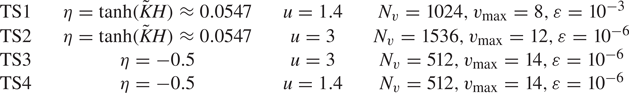
TS1. In this case, the stream velocity is weak ($u=1.4$) so that the charge sector of the dynamics is basically undamped, as seen in figure 9(a) for the electric field. The spin sector is more interesting, both for the ions and the electrons, which are rather strongly damped at a rate ${\approx }6.3 \times 10^{-4}$. This is in contrast with the corresponding Maxwell–Boltzmann simulation (MB1, figure 6) where the spin mode was very weakly damped. Although the wavenumber is not the same ($k=0.5$ for MB1 and $k=0.2$ for TS1), it appears that the equilibrium profile has a strong impact on the stability properties of the ion magnon mode.

Figure 9.

TS1 simulation. (a) Time evolution of the square root of the electric energy ${\mathcal {H}}_E^{1/2}$ (given by (4.2)) for short times $t\in [0, 50]$. (b) Time evolution of the absolute value of the real part of the fundamental mode of the electron spin $\hat {M}_1$. (c) Time evolution of the absolute value of the real part of the fundamental mode of the ion spin $\hat {S}_1$. The red straight lines have slopes equal to zero for the electric energy and $-6.3 \times 10^{-4}$ for $\hat {M}_1$ and $\hat {S}_1$.

TS2. This run uses the same parameters as TS1, except that the stream velocity is larger, $u=3$. We also changed the magnitude of the initial perturbation, now set to $\varepsilon =10^{-6}$, to get a longer-lasting linear phase. Linear theory predicts an instability in the charge sector, with growth rate equal to $0.2845$, which is confirmed by the numerical data shown in figure 10(a). The ion spin sector displays a very weak instability, with an observed growth rate ${\approx }4\times 10^{-5}$. The electron spin remains at very low amplitude all along the simulation time.

Figure 10.

TS2 simulation. (a) Time evolution of the square root of the electric energy ${\mathcal {H}}_E^{1/2}$ (given by (4.2)) for short times $t\in [0, 100]$. (b) Time evolution of the absolute value of the real part of the fundamental mode of the electron spin $\hat {M}_1$. (c) Time evolution of the absolute value of the real part of the fundamental mode of the ion spin $\hat {S}_1$. The red straight lines have slopes equal to $0.2845$ for the electric energy and $4\times 10^{-5}$ for $\hat {S}_1$.

TS3. Here, we wish to consider a case where an instability is expected both in the charge and in the spin sectors. Therefore, we take the same value $u=3$ for the stream velocity as in TS2, and an electron spin polarization $\eta =-0.5$, which leads to the instability of the magnon mode in MB3. The results are plotted in figure 11 and show that the evolution of the electric field is almost the same as in the case TS2. This is natural, as the linear response of the charge sector is independent of $\eta$ (nonetheless, one may have expected some differences after the nonlinear regime is attained, around $\omega _p t= 50$, but in practice, the two curves are very similar, although not identical). Interestingly, the electron $\hat {M}_1$ and ion $\hat {S}_1$ spins are initially stable until $\omega _p t \approx 2500$, i.e. well into the nonlinear regime, and only become unstable later. Their growth rate is much smaller than the one associated with the charges.

Figure 11.

TS3 simulation. (a) Time evolution of the square root of the electric energy ${\mathcal {H}}_E^{1/2}$ (given by (4.2)) for short times $t\in [0, 100]$; the red straight line has slope equal to $0.2845$. (b) Time evolution of the absolute value of the real part of the fundamental mode of the electron spin $\hat {M}_1$. (c) Time evolution of the absolute value of the real part of the fundamental mode of the ion spin $\hat {S}_1$.

The phase space portraits at the end of the simulation are displayed in figure 12 for the four distributions $f_0(t, x, v)$ and $f_\ell (t, x, v), \ell =1, 2, 3$. Typically, for this type of instability, the two-stream structure has been destroyed in the nonlinear regime and a single vortex centred at $v=0$ can be observed. The vortex is present not only in the charge distribution $f_0$, but also in the spin distributions ${\boldsymbol f}$.

Figure 12.

TS3 simulation. Contour plots of the distribution functions in the $(x,v)$ phase space at the final time $\omega _p t=10^4$: (a) $f_0$; (b) $f_1$; (c) $f_2$ and (d) $f_3$.

TS4. Finally, we repeat the same simulation as TS3, but for a smaller stream velocity $u=1.4$, so that there is no instability in the charge sector (see figure 13). In this case, the usual magnon instability ($\eta <0$) develops immediately, in contrast to the preceding TS3 case. Although it is difficult to draw definite conclusions, it is clear that the onset, or otherwise, of a charge instability interacts strongly with the development of a magnon instability. This is further evidence that the charge and spin sectors are closely intertwined and need to be both included in the model for an accurate description of the magnonic dynamics.

Figure 13.

TS4 simulation. (a) Time evolution of the square root of the electric energy ${\mathcal {H}}_E^{1/2}$ (given by (4.2)) for short times $t\in [0, 100]$. (b) Time evolution of the absolute value of the real part of the fundamental mode of the electron spin $\hat {M}_1$. (c) Time evolution of the absolute value of the real part of the fundamental mode of the ion spin $\hat {S}_1$. The red straight lines have slope equal to $0.004$.