


1. Introduction
When a binary alloy is solidified, morphological instability (Mullins & Sekerka Reference Mullins and Sekerka1964) often results in the formation of a reactive porous mushy layer of solid crystals bathed in residual melt (cf. Worster Reference Worster2000). Mushy-layer growth is relevant in industrial, geological and geophysical settings (see reviews by Worster Reference Worster1997; Anderson & Guba Reference Anderson and Guba2020). Examples include the casting of metal alloys (Copley et al. Reference Copley, Giamei, Johnson and Hornbeck1970), solidification in magma chambers and planetary inner cores (Bergman & Fearn Reference Bergman and Fearn1994; Worster Reference Worster2000; Huguet et al. Reference Huguet, Alboussiére, Bergman, Deguen, Labrosse and Lesœur2016) and the growth of sea ice in the polar oceans (Feltham et al. Reference Feltham, Untersteiner, Wettlaufer and Worster2006; Hunke et al. Reference Hunke, Notz, Turner and Vancoppenolle2011; Worster & Rees Jones Reference Worster and Rees Jones2015; Wells, Hitchen & Parkinson Reference Wells, Hitchen and Parkinson2019). In growing mushy layers, solidification occurs at the advancing mush–liquid free boundary, and also via internal porosity changes. The evolving porosity impacts the mechanical, thermal and electromagnetic properties, both during growth and in the composite solid formed by quenching in industrial and geological settings. Evolving porosity also impacts transport through the mushy layer via diffusion, and by moderating the permeability to flow. For example, the porosity and permeability of sea ice moderates convective brine drainage, which provides buoyancy forcing for the polar oceans and drives significant biogeochemical fluxes through the ice interior (Hunke et al. Reference Hunke, Notz, Turner and Vancoppenolle2011; Worster & Rees Jones Reference Worster and Rees Jones2015; Wells et al. Reference Wells, Hitchen and Parkinson2019). Sea-ice porosity also provides a substrate for life within the liquid pore space (Hunke et al. Reference Hunke, Notz, Turner and Vancoppenolle2011). Hence, there is interest in understanding how the mushy-layer structure and transport through mushy layers evolve during transient growth. In a pair of papers, we first assess the impact of the fluid temperature, concentration and cooling conditions on porosity evolution during transient diffusive growth of a mushy layer from a fixed cooled boundary (Part 1, this manuscript). The corresponding impact on the onset and localisation of convective flow instability within a mushy layer is considered in Part 2 (Hitchen & Wells Reference Hitchen and Wells2025).
Diffusively controlled mushy-layer growth (in the absence of convection and externally forced flow) has been considered in a variety of situations (see reviews by Worster Reference Worster1997; Anderson & Guba Reference Anderson and Guba2020). It is relevant to settings where density gradients are stabilising, or prior to the onset of convection where diffusive growth provides a background state about which to assess stability. Two main growth conditions have received most attention (Worster Reference Worster1997). Fixed-chill growth features transient solidification where a deep layer is cooled instantaneously by an isothermal boundary, and results in self-similar ice growth. Meanwhile, directional solidification features steady growth of a sample pulled between fixed isothermal heat exchangers. For fixed-chill experiments, early theoretical and experimental studies (Huppert & Worster Reference Huppert and Worster1985; Worster Reference Worster1986) showed that the mushy-layer thickness  $\hat {h}$ follows the characteristic growth for a Stefan problem with $\hat {h} \propto \sqrt {\kappa \hat {t}}$ for time $\hat {t}$ and thermal diffusivity $\kappa$. The porosity varies with liquid concentration, and increases with distance from the cooling boundary (Worster Reference Worster1986; Shirtcliffe, Huppert & Worster Reference Shirtcliffe, Huppert and Worster1991). The model and experimental comparisons have since been extended to account for convection in the neighbouring fluid, kinetic undercooling and interfacial disequilibrium (Kerr et al. Reference Kerr, Woods, Worster and Huppert1990a,Reference Kerr, Woods, Worster and Huppertb; Worster & Kerr Reference Worster and Kerr1994), expansion or contraction flows due to density changes (Chiareli, Huppert & Worster Reference Chiareli, Huppert and Worster1994) and slow solute diffusion (Gewecke & Schulze Reference Gewecke and Schulze2011a). There have also been a rich set of analyses of convective flows in mushy layers for fixed chill and directional solidification (reviewed by Worster Reference Worster1997; Worster & Rees Jones Reference Worster and Rees Jones2015; Anderson & Guba Reference Anderson and Guba2020). Other cooling conditions studied include a ramped boundary temperature to achieve steady growth (Neufeld & Wettlaufer Reference Neufeld and Wettlaufer2008a,Reference Neufeld and Wettlauferb; Zhong et al. Reference Zhong, Fragoso, Wells and Wettlaufer2012) and periodic modulation of the boundary temperature about a fixed chill (Ding, Wells & Zhong Reference Ding, Wells and Zhong2019a,Reference Ding, Wells and Zhongb). However, in some settings mushy layer growth is forced by imposed heat fluxes, that may vary with the boundary temperature. For example, young sea-ice growth is controlled by a surface energy balance where outgoing longwave and sensible heat fluxes depend on surface temperature (Maykut & Untersteiner Reference Maykut and Untersteiner1971).
The composition of a binary alloy can also significantly impact the mushy-layer growth and structure. A near-eutectic limit (Fowler Reference Fowler1985) has received considerable attention (see Worster (Reference Worster1997, Reference Worster2000), Anderson & Guba (Reference Anderson and Guba2020) and references therein) and was applied to transient growth by Emms & Fowler (Reference Emms and Fowler1994). The near-eutectic limit results in high porosity of order one throughout the depth of the mushy layer, and allows significant simplification of the mathematical analysis. The contrasting limit, far from the eutectic, has received less attention. Using selected case studies, Worster (Reference Worster1986) and Worster (Reference Worster1991) showed that variation of the liquid composition can cause significant changes to the shape of the porosity profiles, and then considered the resulting impact on linear convective instability during directional solidification (Worster Reference Worster1992).
Building on this earlier insight and the results of Hitchen (Reference Hitchen2017), the goal of this paper is to systematically investigate the response of the porosity of a mushy layer to varying cooling conditions and different initial composition and temperature of the liquid, for transient diffusively controlled growth. Specifically, we consider a deep layer of fluid cooled with a Robin boundary condition
 \begin{equation} { k \frac{\partial T}{\partial \hat{z}} = \mathfrak{h} \left(T-T_c\right) \quad \text{at}{\ \hat{z}=0},} \end{equation}
where  $T$ is the local temperature, $\hat {z}$ distance from the boundary, $k$ thermal conductivity of the mushy layer, $\mathfrak {h}$ a constant heat transfer coefficient for the boundary medium and $T_c$ a restoring temperature for the boundary. This type of condition is often recovered from a linearisation of a surface energy balance, such as that controlling sea-ice growth where the heat flux conducted out from the ice depends on outgoing longwave radiative and turbulent sensible heat fluxes, which both depend on the surface temperature (see Appendix A of Hitchen & Wells Reference Hitchen and Wells2016). As an example, in Part 2 we estimate that for parameterised turbulent sensible atmospheric heat fluxes over sea ice with wind speeds between $1$ and $10\ \mathrm {m}\ \mathrm {s}^{-1}$, the length scale ${k}/{\mathfrak {h}}$ is in the range $0.67$ to $0.067\ \mathrm {m}$, decreasing with increasing wind speed. Hence, the corresponding thermal boundary-layer scale in the ice induced by (1.1) can be comparable to the ice thickness as it varies between a few centimetres to over a metre during the initial seasonal ice growth. The condition (1.1) is also relevant for a boundary consisting of a thin cooling plate of thickness $\delta$ and finite conductivity $\mathfrak {h} \delta$ in contact with a large isothermal heat bath (e.g. Hurle, Jakeman & Pike Reference Hurle, Jakeman and Pike1967). A fixed-chill setting with isothermal boundary temperature is recovered when ${\mathfrak {h}}/{k} \rightarrow \infty$, corresponding to a boundary with perfect efficiency of heat transfer. Imperfect boundary heat transfer is obtained for finite ${\mathfrak {h}}/{k}$, and a perfectly insulating boundary occurs when ${\mathfrak {h}}/{k} \rightarrow 0$.
For perfectly conducting boundaries  $({\mathfrak {h}}/{k} \rightarrow \infty )$ we below identify differing regimes depending on the concentration ratio $\mathcal {C}={(\hat {S}_\infty -\hat {S}_s)}/{(\hat {S}_c-\hat {S}_\infty )}$, where $\hat {S}_\infty$ is the initial fluid composition, $\hat {S}_s$ the composition of pure solid and $\hat {S}_c$ is the composition corresponding to liquidus temperature $T_c$. A high-porosity mushy layer is recovered for $\mathcal {C} \gg 1$, as an extension of the traditional near-eutectic limit. For $\mathcal {C} \ll 1$ we find that large porosity gradients are confined to a high porosity boundary layer near the mush–liquid interface, with a low-porosity interior. For boundary cooling with imperfect heat transfer (i.e. finite $\mathfrak {h}$) a corresponding behaviour is obtained after sufficiently long times. However, the impact of boundary cooling varies over time, as characterised by a dimensionless Biot number ${\tilde {\mathcal {B}}_i}={\mathfrak {h} \sqrt {\kappa t }}/{k}$ based on the efficiency of boundary cooling vs thermal conduction across a diffusive boundary-layer scale in the mush. We quantify the initial delay time scale for cooling below freezing, and identify a subsequent transition regime where the porosity varies significantly throughout the depth and over time. At late times the porosity structure approaches the self-similar limit obtained for fixed-chill cooling.
The article is organised as follows. Section 2 describes the model of diffusively controlled growth of a mushy layer. Section 3 considers growth with a perfectly conducting boundary ( $\mathfrak {h} \rightarrow \infty$), whilst § 4 considers the impact of imperfect boundary heat transfer with finite $\mathfrak {h}$. The implications for sea-ice properties are discussed in § 5, with conclusions in § 6.
2. Model
We consider a semi-infinite liquid region, with a uniform initial temperature  $T_\infty$ and salinity $\hat {S}_\infty$. The salinity of the solid phase $\hat {S}_s$ is constant. At $\hat {t} = 0$, the liquid is exposed to a heat sink of temperature $T_c$, with boundary condition (1.1) applied at $\hat {z} = 0$. When the temperature at the surface of the liquid reaches the initial liquidus temperature $T_{L\infty }$ for the fluid of salinity $\hat {S}_\infty$, a porous mushy layer begins to form with thickness $\hat {h}$, as illustrated in figure 1. We will assume that the fluid remains at rest – relevant to statically stable density gradients or examining the growth and structure of the mushy layer before convective onset.
Diagram of the model. The temperature  $T$ approaches $T_\infty$ at depth, and is relaxed towards $T_c$ at the surface with cooling provided via a linearised heat exchange. In the liquid phase, the salinity $\hat {S}_\infty$ is uniform and the liquidus temperature is $T_L=T_{L\infty }$, with both constant due to the neglect of salt diffusion or fluid motion. In the mushy phase, the temperature and salinity are related via the liquidus relationship. The dominant length scale $\sqrt {\kappa \hat {t}}$ is the time-evolving thermal diffusion length.

We apply ideal mushy-layer theory (Worster Reference Worster1986) to describe the reactive porous material formed during the solidification of a binary alloy. This assumes that any pore-scale variations are equilibrated much faster than any macroscopic time of interest, such that local thermodynamic equilibrium holds. Hence, the temperature  $T$ and liquid salinity $\hat {S}$ are locally constrained via a liquidus relationship, $T = T_L(\hat {S})$, and unbalanced fluxes drive change in the volumetric liquid fraction (or porosity) $\chi$. The corresponding solid fraction is $\phi = 1-\chi$. For simplicity, the thermal properties and densities are assumed to be independent of the phase.
Conservation of energy and salt are given by
 \begin{equation} \frac{\partial T}{\partial\hat{t}}+ \frac{L}{c_p} \frac{\partial \chi}{\partial \hat{t}} = \kappa\hat{\nabla}^2T, \quad \frac{\partial\bar{\hat{S}}}{\partial\hat{t}} = \frac{\partial [\chi\hat{S}+(1-\chi)\hat{S}_s ]}{\partial\hat{t}} = 0, \end{equation}
where  $\bar {{\hat {S}}} = \chi \hat {S}+(1-\chi )\hat {S}_s$ is the phase-weighted bulk salinity. We have here neglected salt diffusion because the solute diffusivity, $D$, is much smaller than the thermal diffusivity, $D \ll \kappa$ (see Gewecke & Schulze (Reference Gewecke and Schulze2011b), Hitchen (Reference Hitchen2017) and Wells et al. (Reference Wells, Hitchen and Parkinson2019), for discussion of the effects of salt diffusion). The latent heat is $L$, and the specific heat capacity is $c_p$. Note that (2.1) holds both within the mushy layer, $\chi < 1$, and for the liquid phase, $\chi = 1$.
We model the liquidus as a linear relationship with gradient  $\varGamma$, and use this to express the liquid fraction in terms of the temperature within the mushy region
 \begin{align} T = T_L(\hat{S}) = T_{L\infty} - \varGamma(\hat{S}-\hat{S}_\infty), \quad\chi = \frac{\varGamma(\hat{S}_\infty-\hat{S}_s)}{\varGamma(\hat{S}_\infty-\hat{S}_s) + T_{L\infty} - T_L(\hat{S})} \quad \text{for}\ {0\leqslant\hat{z}\leqslant\hat{h}}, \end{align}
where we have made use of the constant bulk salinity  $\bar {{\hat {S}}} =\hat {S}_\infty$ predicted by (2.1b). Using (2.2) the system is determined by the evolution of the temperature as given by (2.1a).
To complete the model, we need to specify the boundary conditions at the external and internal interfaces. We consider a deep-pool limit, whereby the physical domain depth,  $\hat {b}$, is much larger than the thermal diffusion length scale, $\hat {b}\gg \sqrt {\kappa \hat {t}}$, for any time of interest. The temperature at depth tends towards the initial value
 \begin{equation} {T \rightarrow T_\infty \quad \text{as}\ {\hat{z}\rightarrow\infty}. } \end{equation}
We also assume linearised heat transfer between the surface heat sink and the surface of the mushy layer, as described by (1.1). Under this model the rate of heat loss is directly proportional to the temperature difference between the heat sink and the surface of the mushy layer. Since the surface temperature evolves dynamically over time, the rate of heat loss does too.
The temperature and salinity in the liquid phase are continuous across the mush–liquid interface (Schulze & Worster Reference Schulze and Worster2005) and lie at the liquidus temperature just inside the mush, which leads to
 \begin{equation} T|_+ = T|_- = T_{L\infty}\quad \text{at}\ {\hat{z} = \hat{h}}(\hat{t}), \end{equation}
where we have exploited the constant salinity in the liquid phase. The above imply unit liquid fraction on the mushy side of the interface (Schulze & Worster Reference Schulze and Worster2005), and an energy balance that reduces to continuity of thermal fluxes
 \begin{equation} \chi|_- = 1, \quad \left.\frac{\partial T}{\partial\hat{z}}\right|_+ = \left.\frac{\partial T}{\partial\hat{z}}\right|_-\quad \text{at}\ {\hat{z} = \hat{h}}(\hat{t}). \end{equation}
2.1. Non-dimensionalisation
The thermal diffusion length scale  $\sqrt {\kappa \hat {t}}$ provides a natural scale for non-dimensionalisation, but using a time-evolving scale introduces complexity into the problem from the coordinate transformations. It is therefore convenient for initial non-dimensionalisation and analysis to use a fixed, time-independent length scale $\hat {d}$. This scale can be considered as a physical length scale (such as mixed-layer depth of the ocean or the depth of some experimental apparatus), or the thermal diffusion length after some chosen interrogation time, at which we observe the system. We will scale this distance $\hat {d}$ out of the problem in favour of the thermal diffusion length scale during later stages of the analysis. We non-dimensionalise time via the associated thermal diffusion time scale $\hat {d}^2/\kappa$.
We define the dimensionless temperature and salinities
 \begin{equation} {\theta = \frac{T - T_c}{T_{L\infty} - T_c}, \quad\bar{S} = \frac{\bar{{\hat{S}}}-\hat{S}_s}{\hat{S}_\infty-\hat{S}_s}, \quad S = \frac{\hat{S}-\hat{S}_s}{\hat{S}_\infty-\hat{S}_s} .} \end{equation}
The temperature scale  $\Delta T = T_{L\infty } - T_c$ is the temperature difference from the mush–liquid interface to the surface heat sink. Using these scales, the liquidus relationship (2.2a) and the lever rule (2.2b) become
 \begin{equation} {\theta}_L(S) =1- \mathcal{C} \left(S-1\right), \quad \chi = \frac{\mathcal{C}}{\mathcal{C} + 1 - \theta}, \end{equation}
where we have used the dimensionless concentration ratio
 \begin{equation} {\mathcal{C} \equiv \frac{\varGamma(\hat{S}_\infty-\hat{S}_s)}{T_{L\infty} - T_c} = \frac{\hat{S}_\infty-\hat{S}_s}{\hat{S}_c-\hat{S}_\infty}. } \end{equation}
The concentration ratio  $\mathcal {C}$ in (2.7) is a ratio of salinity differences, but can also be viewed as comparing the size of the freezing point depression $\varGamma (\hat {S}_\infty -\hat {S}_s)$ with the temperature scale and is therefore a measure of the significance of salinity effects for the solidification dynamics. The limit $\mathcal {C}\rightarrow 0$ represents a pure fluid with no salt content. Note that this definition of $\mathcal {C}$ is consistent with that used by some previous studies (Worster Reference Worster1991; Feltham & Worster Reference Feltham and Worster1999; Hwang Reference Hwang2013) but others have used contrasting definitions (e.g. Worster Reference Worster1997).
The boundary conditions at depth (2.3) and the interface (2.4) become
 $$\begin{gather} \theta \rightarrow \theta_{\infty} \quad \text{as}\ {z\rightarrow\infty} , \end{gather}$$
 $$\begin{gather}\theta|_+ = \theta|_- = 1, \quad \left[{\boldsymbol{n}}\boldsymbol{\cdot}\boldsymbol{\nabla}\theta\right]^+_- = 0 \quad \text{at}\ {z=h}, \end{gather}$$
for dimensionless depth  $z$, time $t$, mush thickness $h$ and normal ${\boldsymbol {n}}$. The dimensionless temperature of the far-field liquid is defined as $\theta _{\infty } ={(T_\infty - T_c)}/{(T_{L\infty } - T_c)}$ and satisfies $1< \theta _{\infty }<\infty$, with $\theta _{\infty }-1$ representing the degree to which the far-field liquid is above the liquidus temperature. At the surface, the thermal condition (1.1) yields
 \begin{equation} {\frac{\partial\theta}{\partial z} = {\mathcal{B}_i}\theta \quad \text{at}\ {z = 0}, } \end{equation}
where we have introduced a reference Biot number
 \begin{equation} {{\mathcal{B}_i} = \frac{\mathfrak{h}\hat{d}}{k}.} \end{equation}
The Biot number represents the rate of heat transfer into the heat sink compared with thermal diffusion within the fluid or mushy layer, noting that  $\mathfrak {h}$ could depend on the conductivity of a bounding plate, or arise from linearisation of a more complex boundary condition such as radiative cooling (see discussion in § 1). An infinite Biot number represents a perfectly conducting boundary, while a Biot number of zero represents a perfectly insulating one.
The dimensionless dynamical equations of the system are shown to be
 \begin{equation} {\frac{\partial\theta}{\partial t} + {\mathcal{S}_t}\frac{\partial\chi}{\partial t} = \nabla^2\theta, \quad \frac{\partial\chi S}{\partial t} = 0, } \end{equation}
where the Stefan number,  ${\mathcal {S}_t} = {L}/{c_p(T_{L\infty } -T_c)}$, represents the ratio of latent to specific heat in the system. A larger Stefan number means that the latent heat release from solidification will have a greater impact.
3. Mush with perfect boundary conduction
We first systematically investigate the changes to the growth rate and internal structure of mushy layers in contact with a perfectly conducting boundary ( ${\mathcal {B}_i}\rightarrow \infty$). We expand on the results of Worster (Reference Worster1986) by considering the effect of simultaneous variation of multiple parameters, and providing a more detailed discussion of the internal structure.
3.1. Method
With a perfectly conducting boundary, the problem can be expressed in terms of a self-similar coordinate  ${\tilde {z}} = {z}/{\sqrt {t}}$, which grows with the thermal diffusion length scale. Denoting $\tilde{t} =t$, we seek solutions that only depend on time through ${\tilde {z}}$ and are independent of $\tilde{t}$. Applying this coordinate transformation to the thermal diffusion equation (2.10a) and differentiating the lever rule (2.6b) yields
 \begin{equation} 0 = \frac{\partial^2{\theta}}{\partial{\tilde{z}}^2} + \frac{{\tilde{z}}}{2}\frac{\partial\theta}{\partial{\tilde{z}}} + \frac{{\mathcal{S}_t}{\tilde{z}}}{2}\frac{\partial\chi}{\partial{\tilde{z}}}, \quad \left(\mathcal{C} + 1 - \theta\right)\frac{\partial\chi}{\partial{\tilde{z}}} = \chi\frac{\partial\theta}{\partial{\tilde{z}}}. \end{equation}
In these coordinates the interface position is defined as a constant  $\lambda = {h}/{\sqrt {t}}$. However, since the growth rate is also proportional to the self-similar interface position, ${\partial h }/{\partial t } = {\lambda }/{2\sqrt {t}}$, we will interchangeably refer to this quantity as the scaled growth rate. The boundary conditions applied at ${\tilde {z}} = 0$, ${\tilde {z}}=\lambda$, and as ${\tilde {z}}\rightarrow \infty$ are functionally unchanged from those given in (2.8) with ${\mathcal {B}_i}\rightarrow \infty$ so that $\theta =0$ at ${\tilde {z}}=0$.
We solve this system using a shooting method (Acton Reference Acton1990) after expressing (3.1) as a set of first-order differential equations in  $\theta$, ${\partial \theta }/{\partial {\tilde {z}}}$ and $\chi$. A fourth-order Runge–Kutta method was used to integrate from ${\tilde {z}} = 0$ to an estimated interface position at ${\tilde {z}} = \lambda '$. After applying the boundary conditions at the mush–liquid interface, the integration continues with $\chi$ held at $1$ to some fixed depth that was varied to demonstrate it did not affect the calculation result. The errors on the temperature and liquid fraction at the interface and the far-field temperature were then used to update the boundary conditions at ${\tilde {z}}=0$ and interface position $\lambda$ using the MATLAB function ‘fsolve’, completing the shooting method.
3.2. Results
Figure 2(a) shows that the scaled interfacial growth rate  $\lambda$ increases as the concentration ratio $\mathcal {C}$ increases, but $\lambda$ decreases as the Stefan number ${\mathcal {S}_t}$ increases. When examining the dependence of the growth rate on the liquidus gradient, we observe two regimes of behaviour for small and large $\mathcal {C}$. For $\mathcal {C}\gg 1$ we see that $\lambda$ increases significantly with $\mathcal {C}$. Physically, a larger concentration ratio implies a tendency for stronger depression of the freezing point by salinity and thus requires a smaller change in the salinity of the interstitial liquid to maintain local thermodynamic equilibrium for a given temperature change. This leads to less solidification and segregation of salt into the liquid phase. The decreased internal solidification decreases the amount of latent heat released, which then increases the growth rate of mush thickness. This can also be seen by examining the lever rule (2.6b), and noting that increasing $\mathcal {C}$ will decrease the significance of the $1-\theta$ term, leading to less variation of $\chi$ and less latent heat release. However, in the other regime, where $\mathcal {C}\ll 1$, we observe that the growth rate becomes approximately independent of $\mathcal {C}$. For small concentration ratio, the salinity-dependent freezing point depression is relatively small, so the layer has substantial internal solidification with the lever rule (2.6b) yielding $\chi \ll 1$ throughout most of the depth. Hence the total latent heat release and growth rate hardly vary with $\mathcal {C}$.
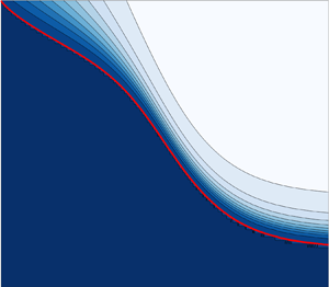
(a) The scaled mushy-layer growth rates  $\lambda$ calculated as a function of the concentration ratio, $\mathcal {C}$, and Stefan number, ${\mathcal {S}_t}$, for $\theta _{\infty } = 2.0$. Solid black contours show growth rate $\lambda \in \{0.1,0.3,0.5,0.7,0.9\}$. Increasing the concentration ratio increases the mush growth rate, whilst increasing the Stefan number decreases the growth rate. For $\mathcal {C} \ll 1$ growth depends predominantly on the thermal Stefan number ${\mathcal {S}_t}$, but for $\mathcal {C} \gg 1$ contours of constant growth rate depend on the compositional Stefan number, ${\mathcal {S}_c} = {\mathcal {S}_t}/\mathcal {C}$. While the position of the growth rate contours varies with $\mathcal {C}$ their spacing does not vary. (b) The mushy-layer growth rates against $\mathcal {C}$ and $\theta _{\infty }$ for ${\mathcal {S}_t} = 15.8$. The red line $\mathcal {C}= 0.3$ roughly indicates the inflection points of the contours of constant growth rate, and the inferred transition between the Stefan limit and the high-liquid-fraction limit discussed in the main text.

The decrease in growth rate as the Stefan number increases occurs because more latent heat is being released by solidification which slows cooling and hence growth. We will not present the details here, but Hitchen (Reference Hitchen2017) demonstrated that the dependence on the Stefan number follows the same functional form as in the two-phase Stefan problem with pure solid and liquid regions. The curves of  $\lambda$ vs ${\mathcal {S}_t}$ generated for this problem can be collapsed onto the original solution with a high degree of accuracy through the use of a multiplicative prefactor for ${\mathcal {S}_t}$ which contains all the dependency on $\mathcal {C}$ and $\theta _{\infty }$. This idea is explored further in § 3.3.3c of Hitchen (Reference Hitchen2017).
Figure 2(b) shows that increasing the dimensionless far-field liquid temperature  $\theta _{\infty }$ decreases the growth rate of the mushy layer for all values of $\mathcal {C}$. A larger value of $\theta _{\infty }-1$ increases the amount of sensible heat which needs to be removed to cool a parcel of fluid to the point where it begins to solidify, which inhibits mushy layer growth. Similarly to figure 2(a), figure 2(b) shows distinct behaviour for small and large $\mathcal {C}$, with the growth rate being almost independent of $\mathcal {C}$ for small $\mathcal {C}$, and showing a transition between limiting behaviours for $\mathcal {C}\approx 0.3$.
The growth rate trends in figure 2(b) can also be compared with Huppert & Worster (Reference Huppert and Worster1985) and Worster (Reference Worster1986). Both studies observed (experimentally and analytically respectively) that increasing the initial fluid concentration  $\hat {S}_\infty$ decreases the growth rates of the mushy layer. This will increase the concentration ratio $\mathcal {C}={\varGamma (\hat {S}_\infty -\hat {S}_s)}/{(T_{L\infty }-T_c)}$, which provides a tendency to increase the growth rate as less solid forms and less latent heat is released. However, $\theta _{\infty }={(T_\infty -T_c)}/{(T_{L\infty }-T_c)}$ also increases because $T_{L\infty }$ decreases. This drives a tendency for the growth rate to decrease because more sensible heat must be removed from fluid parcels before they can solidify. We conclude that the increased removal of sensible heat has a greater impact on the growth rate than the decreased removal of latent heat for the parameter values used in the studies of Huppert & Worster (Reference Huppert and Worster1985) and Worster (Reference Worster1986), where the concentration is varied for constant temperatures.
The two dynamical regimes seen in figure 2 for small and large  $\mathcal {C}$ correspond to separate asymptotic regimes for the mush structure, as illustrated by examining variation of the liquid fraction $\chi ({\tilde {z}})$ with $\mathcal {C}$ in figure 3. We explore the relevant asymptotic limits in greater depth in Appendix A, but key features can be understood by considering the surface liquid fraction
 \begin{equation} {\chi(0) = \frac{1}{1+1/\mathcal{C}}, } \end{equation}
which is found from (2.6b) by setting  $\theta =0$, and depends only on the concentration ratio $\mathcal {C}$. The liquid fraction will be lowest at the surface and $\chi \rightarrow 1$ at the mush–liquid interface, so this allows us to place an upper bound on the internal solidification which occurs.
Liquid-fraction profiles  $\chi$ at a range of concentration ratios for ${\mathcal {S}_t} = 8.0$ and $\theta _{\infty } = 2.0$. (a) The vertical axis is the self-similar depth of the system with the black curve representing the mush–liquid interface. Thick grey contours show $\chi \in \{0.1,0.3,0.7,0.9\}$, the red contour shows $\chi = 0.5$ and the pure liquid region is shaded in light grey. (b) To illustrate the boundary-layer scaling, the vertical axis has been scaled by the mushy-layer depth, ${(\lambda -{\tilde {z}})}/{\lambda }$, and is displayed on a logarithmic scale. The liquid-fraction data have also been rescaled ${[\chi ({\tilde {z}})-\chi (0)]}/{[1-\chi (0)]}$ such that the scaled liquid fraction takes a value of zero at the surface and one at the interface. The solid red curve represents the $\chi = 0.5$ contour, the solid orange curve represents a value of $0.5$ on the compensated scale and the dashed orange curve is the limiting trend of $(1-{{\tilde {z}}}/{\lambda })\sim 2.0\mathcal {C}$. (c) Selected liquid-fraction profiles as a function of depth, for various $\mathcal {C}$.

For large concentration ratio with  $\mathcal {C}\gg 1$, the liquid fraction at the surface $\chi (0) \approx 1-1/\mathcal {C}$. Hence, the liquid fraction $\chi$ is close to $1$ and the solid fraction is small throughout the mush, as seen for large $\mathcal {C}\gg 1$ in figure 3(a). Using the red $\chi = 0.5$ contour to roughly indicate the low-solid-fraction regions (bluer) and high-solid-fraction regions (whiter), we can see that for $\mathcal {C}> 1$ the whole mushy layer is less than $50\,\%$ solidified. As discussed in Appendix A.1 this is almost the same as the well-studied near-eutectic limit (see Fowler (Reference Fowler1985); and studies discussed in Wells et al. Reference Wells, Hitchen and Parkinson2019). However, instead of considering small deviations from a boundary composition at the eutectic point, we here have small deviations of composition from the liquidus salinity $\hat {S}_c$ that corresponds to the boundary temperature $T_c$. With a large concentration ratio the imposed temperature changes across the mush require only small deviations in liquid salinity within the pore space to maintain local thermodynamic equilibrium. Hence only a small amount of internal solidification and segregation is required to generate the necessary salinity gradient.
The opposing limit has  $\mathcal {C}\ll 1$, and the surface liquid fraction becomes $\chi (0) \approx \mathcal {C}$. The liquid fraction varies between this small value and $\chi =1$ over the depth of the mush, so here there is substantial variation of $\chi$. Figure 3 shows that for $\mathcal {C}\ll 1$ the upper part of the mush has relatively high solid fraction (small $\chi$), with a thin boundary layer of low solid fraction in the lower part of the mush.
To better illustrate the boundary-layer structure, figure 3(b) shows a compensated version of figure 3(a), with depths scaled by the mushy-layer depth and the liquid fraction scaled by the change in liquid fraction between the interface and the surface. The size of the region of high liquid fraction decreases rapidly as  $\mathcal {C}$ decreases. Introducing the half-solidification depth $f_{\chi }$ as the fraction of the mushy layer depth which has liquid fraction $\chi \geqslant 0.5$, we find the approximate scaling
 \begin{equation} {f_{\chi} = 2.0 \,\mathcal{C}, } \end{equation}
for  $\theta _{\infty }=2$ and ${\mathcal {S}_t} = 8$ (see orange line in figure 3b). In Appendix A.2 we consider the particular asymptotic limit with $\mathcal {C}\ll 1$ and ${\mathcal {S}_t} \mathcal {C} \lesssim 1$. This predicts that the leading-order mush structure consists of an interior region of low liquid fraction with $\chi \ll 1$, with rapid variation of $\chi$ and release of latent heat in a high-porosity boundary layer of relative thickness $(\lambda - {\tilde {z}})/\lambda =O(\mathcal {C})$. This structure is consistent with the scaling seen in figure 3(b) and (3.3). The vast majority of solidification occurs within this boundary layer near the mush–liquid interface. As $\mathcal {C}\rightarrow 0$ this boundary layer becomes vanishingly small, and the liquid fraction jumps from $1$ to $0$ at the interface. This qualitatively resembles the classic two-phase Stefan problem for pure solid growth into a pure fluid separated by a sharp solidification interface. Indeed, Hitchen (Reference Hitchen2017) numerically found that the scaled growth rate quantitatively approaches that of the classical Stefan problem as $\mathcal {C}\rightarrow 0$, with ${<}10\,\%$ difference for $\mathcal {C} <0.04$. We will therefore refer to the regime $\mathcal {C}\ll 1$ as the Stefan limit.
Figure 4 shows that there is a similar pattern of variation of the liquid-fraction profiles with  $\mathcal {C}$ for different far-field liquid temperatures $\theta _{\infty }$. The depth axis has been scaled by a factor of ${\mathcal {S}_t}^{-1/2}$, which is proportional to the leading-order scaling (A10) for the mush thickness in the Stefan limit (see analysis in Appendix A.2). The behaviour is similar for $\mathcal {C}\ll 1$ across all panels, suggesting a similar leading-order behaviour of mushy-layer growth in the Stefan limit, across a range of $\theta _{\infty }$. The red $\chi =1/2$ contour follows a similar pattern in all plots and indicates a transition between regions of low and high liquid fraction. The most pronounced difference is the change to the growth rate when $\mathcal {C}$ approaches $1$ and the Stefan limit breaks down, as indicated by the changing thickness of the mushy layer. The growth rate increases more substantially for smaller $\theta _{\infty }$, consistent with behaviour discussed above for figure 2(b) for $\mathcal {C} \gg 1$. There is also some modest variation in the mush thickness with $\theta _{\infty }$ for small $\mathcal {C}$.
Scaled vertical liquid-fraction profiles for a range of  $\mathcal {C}$, ${\mathcal {S}_t} = 15.8$, and (a) $\theta _{\infty } = 5.0$, (b) $\theta _{\infty } = 2.0$ and (c) $\theta _{\infty } = 1.1$. Solid curves are contours of constant liquid fraction with increment $-0.1$, starting at the mush–liquid interface, with the red curve highlighting the $\chi = 0.5$ contour. The pure liquid region is shaded in light grey. All three graphs are plotted with the same horizontal and colour scales, with depth scaled by ${\tilde {z}}{\mathcal {S}_t}^{1/2}$ appropriate for the leading-order mush thickness scaling for $\mathcal {C}\ll 1$. The changes to the bottom edge of the solid-fraction profiles also indicate the changes to the growth rate as the conditions are varied.

Figures 3 and 4, as well as the asymptotic scalings in Appendix A, support that the transition in mush structure depends on the concentration ratio  $\mathcal {C}={\varGamma (\hat {S}_\infty -\hat {S}_s)}/ {(T_{L\infty }-T_c})$. The link between $\mathcal {C}$ and the liquid fraction was identified in Worster (Reference Worster1991) for steady directional solidification. This combination represents the ratio of the freezing point depression, $\varGamma (\hat {S}_\infty -\hat {S}_s)$, to the temperature difference across a perfectly cooled mushy layer, $T_{L\infty }-T_c$, and the behaviour it governs is summarised in table 1. When the freezing point depression is much larger than the temperature difference across the mushy layer, $\mathcal {C}$ is large. The mushy layer is mostly liquid because only a small amount of solidification needs to occur before the salinity has been restored to local thermodynamic equilibrium. However, when the temperature difference across the mushy layer is much larger than the freezing point depression, $\mathcal {C}$ is small. The mushy layer is mostly solid with a small mushy interface region because much larger amounts of solid must be formed (and larger amounts of salt rejected) to maintain local thermodynamic equilibrium.
The regimes identified for mushy-layer growth from a perfectly conducting boundary. The transition scaling  $\mathcal {C} \approx 0.3$ is identified from figure 2(b). Appendix A.2 derives scalings for the scaled mushy-layer thickness $\lambda$ and fraction $f_{\chi }$ of the mush depth in a high-porosity boundary layer in the Stefan limit, whilst the regime with high liquid fraction recovers governing equations similar to the well-studied near-eutectic limit (Fowler Reference Fowler1985) where the scaled mush thickness depends only on an effective heat capacity $\varOmega =1+{\mathcal {S}_t}/\mathcal {C}$ and scaled liquidus temperature of the far-field fluid. For brevity, we set $\hat {S}_s=0$ above.

Parallels can be drawn with figure 12 of Aussillous et al. (Reference Aussillous, Sederman, Gladden, Huppert and Worster2006) in their study of solidifying a water–sucrose mixture that made use of magnetic resonance imaging (MRI) imaging to measure the internal solidification. They show experimentally measured liquid-fraction profiles against depth for four different initial salinities, with a decrease in internal solidification as the initial salinity increases. Increasing the initial salinity  $\hat {S}_\infty$ for fixed temperatures will increase $\mathcal {C}$ and figures 3 and 4 show this results in a decrease in internal solidification, agreeing qualitatively with the experimental observations of Aussillous et al. (Reference Aussillous, Sederman, Gladden, Huppert and Worster2006).
The asymptotic regimes identified in Appendix A lead to predictions for the growth rate which are evaluated in figure 5. In the well-studied low-solid-fraction limit (cf. Fowler Reference Fowler1985) with  $\mathcal {C}\gg 1$, the growth rate is predicted to approximately depend on an effective heat capacity $\varOmega =1+{\mathcal {S}_t}/\mathcal {C}$ and $\theta _{\infty }$ at leading order, according to (A6). Solutions of (A6) are plotted as solid curves as a function of $\varOmega$ in figure 5(a). Symbols show data points for calculations of the full model with a range of parameter combinations sampled from figure 2 with $\mathcal {C}\geqslant 5$, which show an excellent collapse onto the predicted asymptotic scaling given by (A6). Note that the plotted star symbols correspond to varying $\mathcal {C}$ and $\theta _{\infty }$ with ${\mathcal {S}_t}$ held fixed, and hence the relevant data points cluster towards small $\varOmega =1+{\mathcal {S}_t}/\mathcal {C}$ for large $\mathcal {C}$. The scaling $\lambda (\varOmega,\theta _{\infty })$ is also consistent with behaviour for large $\mathcal {C}$ in figure 2(a), where contours of constant growth rate with fixed $\theta _{\infty }$ align with contours ${\mathcal {S}_c}={\mathcal {S}_t}/\mathcal {C} \sim \mathrm {constant}$ or equivalently $\varOmega \sim \mathrm {const}$.
Variation of the mush growth rate  $\lambda$ with (a) effective heat capacity $\varOmega =1+{\mathcal {S}_t}/\mathcal {C}$ in the low-solid-fraction limit with $\mathcal {C} \gg 1$, and (b) ${\mathcal {S}_t}^{-1/2}$ in the Stefan regime with $\mathcal {C} \ll 1$. In (a) solid curves show approximate theoretical solutions of the simplified model (A6) for different $\theta _{\infty }$. Symbols show corresponding data points with $\mathcal {C} \geqslant 5$ for full calculations sampled from figure 2(a) with $\theta _{\infty }=2$ (circles) and figure 2(b) with ${\mathcal {S}_t}=15.8$ (stars with symbol colour indicating $\theta _{\infty }$). In (b) data points are sampled from figure 2(a) in the Stefan limit with $\mathcal {C}\leqslant 1/5$, with symbol colour indicating the value of $\mathcal {C}$, as shown in the colour bar. A line of best fit to data with $\mathcal {C}=0.002$, $\theta _{\infty }=2$ and ${\mathcal {S}_t}>280$ is plotted in red in (b), consistent with the predicted asymptotic scaling (A10) for small $\mathcal {C}$ and ${\mathcal {S}_t}^{-1/2} \ll 1$ from Appendix A.2.

Figure 5(b) considers the Stefan limit, with  $\mathcal {C}\ll 1$, plotting growth rate $\lambda$ as a function of ${\mathcal {S}_t}^{-1/2}$ for data sampled from figure 2(a) with $\mathcal {C} \leqslant 1/5$. Equation (A10) predicts that the growth rate $\lambda \sim \alpha {\mathcal {S}_t}^{-1/2}$ when $\mathcal {C} \ll 1$, ${\mathcal {S}_t} \mathcal {C} \lesssim 1$ and ${\mathcal {S}_t}^{-1/2} \lesssim 1$, where the prefactor $\alpha$ asymptotes to a constant for small enough $\mathcal {C}$ with ${\mathcal {S}_t}\mathcal {C} \ll 1$. The data for ${\mathcal {S}_t}^{-1/2} \ll 1$ are broadly consistent with the suggested linear scaling, with the red line $\lambda \sim 1.4 {\mathcal {S}_t}^{-1/2}$ representing a linear fit to data with the smallest $\mathcal {C}$, where we expect the scaling to hold best. As in the low- $\mathcal {C}$ limit of figure 4 there is some variation about this trend, likely due to $\alpha$ depending on ${\mathcal {S}_t}\mathcal {C}$ as suggested in Appendix A.2. The linear scaling breaks down as ${\mathcal {S}_t}^{-1/2}$ approaches $1$, and there is a cross-over to a new regime for ${\mathcal {S}_t}^{-1/2} \gg 1$. This is expected because the assumptions underlying the calculation in Appendix A.2 break down for ${\mathcal {S}_t}^{-1/2} \gg 1$. The scaling $\lambda \sim \alpha {\mathcal {S}_t}^{-1/2}$ is also consistent with the observation in figure 2(a) that the growth rate becomes independent of $\mathcal {C}$ for small $\mathcal {C}$.
4. Mush with an imperfectly conducting boundary
We now consider the case of an imperfectly conducting boundary, as represented by (2.8d) with a finite Biot number. Unlike the perfectly conducting case with infinite Biot number, the temperature at the surface of the mushy layer responds to the initial change in thermal forcing on a finite time scale, given by  ${1}/{{\mathcal {B}_i}^2}$ in dimensionless form, rather than instantaneously. This represents a departure from previous studies of mushy-layer growth, either in this setting or in the directional solidification problem.
4.1. Method
We will use two different methods to investigate the effects of imperfect boundary conduction. The first uses a direct numerical integration of the dynamical equations, while the second considers approximate solutions of the simplified model for relatively low solid fraction. This latter method builds on the approximation and solution discussed in Hitchen (Reference Hitchen2017), which produces an analytical solution for the whole domain by combining solutions for the mushy and liquid layers, with results presented here being an extension of the model in Wells et al. (Reference Wells, Hitchen and Parkinson2019) to account for finite Biot number.
When interpreting the results, we consider the rescaled coordinate  ${\tilde {z}}=z/\sqrt {t}$ with depth scaled by the thermal diffusion length. This led to a self-similar solution when ${\mathcal {B}_i} \rightarrow \infty$ in § 3, but for finite ${\mathcal {B}_i}$ we retain an additional dependency on time through the self-similar Biot number, ${\tilde {\mathcal {B}}_i} = {\mathcal {B}_i}\sqrt {t}$ corresponding to the diffusion length scaled by the length scale $k/\mathfrak {h}$ arising from the boundary condition (1.1). We present results using the quasi-self-similar $({\tilde {z}},{\tilde {\mathcal {B}}_i})$-coordinates below. The self-similar Biot number becomes a proxy for the time evolution of any given physical system, noting that there will also be a spread in the vertical coordinate as the thermal diffusion length scale grows. These coordinates could also be interpreted as comparing results at $t = 1$ for different Biot numbers.
4.1.1. Numerical method
The numerical method combines the thermal and salinity equations (2.10) in the mush, as well as the lever rule (2.6b) to eliminate the liquid salinity and liquid fraction in favour of the temperature
 \begin{equation} c_{eff} \frac{\partial\theta}{\partial t} = \frac{\partial^2\theta}{\partial z^2}, \quad c_{eff} = 1 + \frac{{\mathcal{S}_t}\mathcal{C}}{\left(\mathcal{C} + 1 - \theta\right)^2} . \end{equation}
This is now a standard diffusion equation with a variable dimensionless heat capacity  $c_{\rm eff}(\theta )$ and the dimensionless conductivity is $1$.
$1$.
The system (4.1) is solved for a fixed-depth box using the Matlab ‘pdepe’ partial differential equation routine. The whole depth is treated as one domain by leveraging the enthalpy method and providing the heat capacity  $c_{eff}$ for $\theta \leqslant 1$ and a value of $c_{eff}=1$ otherwise (i.e. in the liquid). Integrations were performed from a uniform initial state and a box sufficiently deep for the results not to depend significantly on the box depth, for a variety of Biot numbers. Results from each run and at different times are then combined by rescaling the vertical coordinate by the time-evolving thermal diffusion length scale, and calculating the corresponding self-similar Biot number. The computation was benchmarked against both the shooting method of § 3.1 for infinite Biot number, and also compared with the simplified model below for the high-liquid-fraction regime.
4.1.2. Approximate solution with high liquid fraction
We also consider an asymptotically simplified solution in a generalisation of the near-eutectic limit (cf. Fowler Reference Fowler1985) where  $\mathcal {C} \gg 1 - \theta$, resulting in a high liquid fraction $\chi \approx 1 - {(1-\theta )}/{\mathcal {C}}$ which is close to one. Hence (4.1a) applies, but with effective heat capacity $c_{eff} \approx \varOmega = 1 + {\mathcal {S}_t}/\mathcal {C}$ in the mushy layer and $c_{eff} =1$ in the liquid.
Prior to reaching the freezing temperature, the liquid temperature is described by the solution to the heat equation (4.1a) with  $c_{eff} =1$, and boundary conditions (2.8a,d). This yields
 \begin{equation} \theta =\theta_{\infty}\, f({\tilde{z}},{\tilde{\mathcal{B}}_i}), \quad
f({\tilde{z}},{\tilde{\mathcal{B}}_i}) \equiv
\mathrm{erf}\left({\frac{{\tilde{z}}}{2}}\right) +
\exp{\biggl(\frac{-{\tilde{z}}^2}{4}\biggr)}\,{\rm
erfcx}\left({\frac{{\tilde{z}}}{2}+{\tilde{\mathcal{B}}_i}}\right),
\end{equation}
\begin{equation} \theta =\theta_{\infty}\, f({\tilde{z}},{\tilde{\mathcal{B}}_i}), \quad
f({\tilde{z}},{\tilde{\mathcal{B}}_i}) \equiv
\mathrm{erf}\left({\frac{{\tilde{z}}}{2}}\right) +
\exp{\biggl(\frac{-{\tilde{z}}^2}{4}\biggr)}\,{\rm
erfcx}\left({\frac{{\tilde{z}}}{2}+{\tilde{\mathcal{B}}_i}}\right),
\end{equation}
(see Carslaw & Jaeger (Reference Carslaw and Jaeger1959), for example) where we have defined the function  $f({\tilde {z}},{\tilde {\mathcal {B}}_i})$ for later use. Here, $\mathrm {erfcx}(y) = \exp ({y^2})\,\mathrm {erfc}(y)$ is the scaled complimentary error function, with $\mathrm {erfc}(y)=1-\mathrm {erf}(y)$ and $\mathrm {erf}(y) = (2/\sqrt {{\rm \pi} })\int _0^{y} \exp (-u^2)\, {\rm d}u$. The imperfect cooling at the upper boundary causes a delay in cooling characterised by the ${\tilde {\mathcal {B}}_i}$ dependent terms in $f({\tilde {z}},{\tilde {\mathcal {B}}_i})$. This solution holds until the upper surface reaches the freezing temperature, with $\theta _{\infty }f(0,\widetilde {\mathcal {B}_f})=1$ at the freezing Biot number ${\tilde {\mathcal {B}}_i}=\widetilde {\mathcal {B}_f}$ (or equivalently freezing time $t=t_f$).
Following the onset of freezing, heat transfer within the growing mushy layer instead satisfies (4.1a) with  $c_{eff} \approx \varOmega$. We exploit a heuristic approximation to the temperature for $t\geqslant t_f$, which matches the liquid temperature at $t=t_f$ and recovers the correct asymptotic behaviour for large heat capacity $(\varOmega \gg 1)$ and sufficiently large ${\tilde {\mathcal {B}}_i}$ (as derived in Appendix B and discussed below). We set
 $$\begin{gather} \theta = \frac{f({\tilde{z}} \sqrt{\varOmega},{\tilde{\mathcal{B}}_i}/\sqrt{\varOmega})}{f(\lambda \sqrt{\varOmega},{\tilde{\mathcal{B}}_i}/\sqrt{\varOmega})} \quad\mbox{for} \ 0<{\tilde{z}}< \lambda, \end{gather}$$
 $$\begin{gather}\theta =\theta_{\infty}+ (1-\theta_{\infty}) \biggl[\frac{1- f({\tilde{z}},{\tilde{\mathcal{B}}_i})}{1- f(\lambda,{\tilde{\mathcal{B}}_i})}\biggr] \quad\mbox{for} \ \lambda < {\tilde{z}} <\infty, \end{gather}$$
where the scaled mush thickness  $\lambda = h(t)/\sqrt {t}$ satisfies
 \begin{equation} {\biggl[
\frac{\mathrm{erfcx}({\lambda/2})}{\mathrm{erfcx}({\lambda/2+{\tilde{\mathcal{B}}_i}})}
- 1 \biggr] =(\theta_{\infty} - 1 ) \biggl[
\frac{\mathrm{erf}({\lambda\sqrt{\varOmega}/2})
\exp({\lambda^2\varOmega/4})}{\mathrm{erfcx}({\lambda \sqrt{\varOmega}/2+{\tilde{\mathcal{B}}_i}/\sqrt{\varOmega}})}
+ 1 \biggr],} \end{equation}
\begin{equation} {\biggl[
\frac{\mathrm{erfcx}({\lambda/2})}{\mathrm{erfcx}({\lambda/2+{\tilde{\mathcal{B}}_i}})}
- 1 \biggr] =(\theta_{\infty} - 1 ) \biggl[
\frac{\mathrm{erf}({\lambda\sqrt{\varOmega}/2})
\exp({\lambda^2\varOmega/4})}{\mathrm{erfcx}({\lambda \sqrt{\varOmega}/2+{\tilde{\mathcal{B}}_i}/\sqrt{\varOmega}})}
+ 1 \biggr],} \end{equation}
from the continuity of temperature gradients at the mush–liquid interface (2.8c). For each  ${\tilde {\mathcal {B}}_i}$ we solve (4.4) for $\lambda$ using the Matlab ‘fzero’ routine. The approximation (4.3) satisfies the boundary conditions (2.8) and matches the liquid temperature (4.2) at initial freezing because (4.4) yields $\lambda \rightarrow 0$ as ${\tilde {\mathcal {B}}_i}\rightarrow \widetilde {\mathcal {B}_f}$, and $f(0,\widetilde {\mathcal {B}_f})=1/\theta _{\infty }$. The approximation (4.3) is not, however, an exact solution of (4.1a). Whilst $\theta =A\, f({\tilde {z}} \sqrt {\varOmega }, {\tilde {\mathcal {B}}_i}/\sqrt {\varOmega })$ satisfies (4.1a) with $c_{eff} =\varOmega$ and constant $A$, here $A=1/f(\lambda \sqrt {\varOmega },{\tilde {\mathcal {B}}_i}/\sqrt {\varOmega })$ may implicitly depend on time through $\lambda$ and ${\tilde {\mathcal {B}}_i}$. Similarly $\theta =B\, f({\tilde {z}},{\tilde {\mathcal {B}}_i})+C$ satisfies (4.1a) with $c_{eff} =1$ and constants $B$ and $C$, but $B=1/[ 1- f(\lambda,{\tilde {\mathcal {B}}_i}) ]$ depends implicitly on time. Hence, the approximation (4.3) is not formally justified during the period of rapid mush growth immediately following first freezing when $A$ and $B$ vary significantly with time. Nevertheless, we below find that (4.3) is a good approximation to the full numerical solution for large $\varOmega$ because it matches the exact form of $\theta$ at $t=t_f$, and then at later times $A$ and $B$ are approximately constant for $\varOmega \gg 1$ and sufficiently large ${\tilde {\mathcal {B}}_i}$. For example, for the parameter values in figure 6, we calculate the $L_2$ norm over $0\leqslant \tilde {z} \leqslant 2$ of the difference between the approximate solution (4.3) and a full numerical solution for $\theta$. This yields error that peaks at ${\approx }9\,\%$ of the norm of the numerical solution shortly after onset of freezing, before soon reducing to ${\approx }1\,\%$ for much of the rest of the integration.
The evolution of liquid fraction  $\chi$ for a mushy layer in the high-liquid-fraction regime, plotted against scaled depth ${\tilde {z}}=z/\sqrt {t}$ and self-similar Biot number ${\tilde {\mathcal {B}}_i} = {\mathcal {B}_i} \sqrt {t}$ which increases over time or with increasing efficiency of heat loss at the boundary. Profiles are calculated via numerical solution of (4.1) for $\mathcal {C} = 12.5$, $\theta _{\infty }= 1.25$ and ${\mathcal {S}_t} = 125$. The mush–liquid interface is shown as a solid red line. The red dashed line shows the mush thickness calculated from the approximate solution (4.4). Three distinct periods are visible (separated by grey dashed lines): no solidification for ${\tilde {\mathcal {B}}_i}\leqslant 0.21$, an adjustment region for $0.21\leqslant {\tilde {\mathcal {B}}_i}\lesssim 100$ and a self-similar region for $100\lesssim {\tilde {\mathcal {B}}_i}$ where $\chi$ becomes independent of ${\tilde {\mathcal {B}}_i}$.

4.1.3. Asymptotic behaviour for large effective heat capacity
In the previous section, we set out an approximate solution for mushy-layer growth in the limit of low solid fraction and an imperfectly conducting boundary, which relies on an assumption that the scaled mush growth rate  $\lambda$ does not vary strongly over time. This assumption is justified at late times and the growth rate is zero at early times before mushy-layer growth, but the assumption is harder to rigorously justify during the intermediate adjustment period. Despite this, the approximate solution yields decent quantitative agreement with full numerical solutions. In this section we build understanding of the heuristic approximate solution from § 4.1.2 by considering the behaviour for $\mathcal {C}\gg 1$ and with large heat capacity $\varOmega \gg 1$. This limit facilitates a formal asymptotic solution from a boundary-layer analysis of (4.1a) with $c_{eff} \approx \varOmega$ in the mush and $c_{eff} \approx 1$ in the liquid (see Appendix B). As discussed below we find consistent behaviour of both of the heuristic approximate solution (4.3) and (4.4) and the formal asymptotic solution of Appendix B for $\varOmega \gg 1$. This provides additional support for the heuristic approximation (4.3) and (4.4), and insight into why it appears to capture the main behaviour.
For  $\varOmega \gg 1$, the large heat capacity within the mushy layer slows the diffusive thermal spread, and the asymptotic solution in Appendix B shows that rapid temperature variation is confined to a thermal boundary layer over a scale ${\tilde {z}}=z/\sqrt {t}=O( \varOmega ^{-1/2})$, before saturating as the mush–liquid interface is approached with scale $\lambda =h/\sqrt {t}=O( \varOmega ^{-1/2} \sqrt {\log [\varOmega ^{1/2}]})$. In the limit $\varOmega \gg 1$, the resulting mush thickness is small with $\lambda \ll 1$, but still significantly larger than the narrow diffusive length scale in the mush, with $\lambda \sqrt {\varOmega } \gg 1$. We show below that (4.4) recovers similar behaviour for the growth rate $\lambda$, and (4.3) approaches the asymptotic behaviour derived in Appendix B for $\varOmega \gg 1$.
Using the asymptotic approximations  $\mathrm {erf}(y)\sim 1 - \mathrm {e}^{-y^2}/y\sqrt {{\rm \pi} }$ and $\mathrm {erfcx}(y) \sim 1/y\sqrt {{\rm \pi} }$ for $y\gg 1$, the corresponding dominant balance of (4.4) with $\lambda \ll 1$, $\lambda \sqrt {\varOmega }\gg 1$ and ${\tilde {\mathcal {B}}_i} \gg 1$ yields
 \begin{equation} \frac{
{\tilde{\mathcal{B}}_i}}{\theta_{\infty}-1} \sim
\exp\left({\frac{\lambda^2 \varOmega}{4}} \right)\biggl[
\frac{\lambda \sqrt{\varOmega}}{2} +
\frac{{\tilde{\mathcal{B}}_i}}{\sqrt{\varOmega}}\biggr].
\end{equation}
\begin{equation} \frac{
{\tilde{\mathcal{B}}_i}}{\theta_{\infty}-1} \sim
\exp\left({\frac{\lambda^2 \varOmega}{4}} \right)\biggl[
\frac{\lambda \sqrt{\varOmega}}{2} +
\frac{{\tilde{\mathcal{B}}_i}}{\sqrt{\varOmega}}\biggr].
\end{equation}
The leading-order behaviour can be analysed by taking logarithms, to yield
 \begin{equation}
{\frac{\lambda^2 \varOmega}{4} \sim \log{\biggl(\frac{{\tilde{\mathcal{B}}_i}}{\theta_{\infty}-1}\biggr)}
- \log{\biggl(\frac{\lambda \sqrt{\varOmega}}{2} +
\frac{{\tilde{\mathcal{B}}_i}}{\sqrt{\varOmega}}\biggr)}, }
\end{equation}
\begin{equation}
{\frac{\lambda^2 \varOmega}{4} \sim \log{\biggl(\frac{{\tilde{\mathcal{B}}_i}}{\theta_{\infty}-1}\biggr)}
- \log{\biggl(\frac{\lambda \sqrt{\varOmega}}{2} +
\frac{{\tilde{\mathcal{B}}_i}}{\sqrt{\varOmega}}\biggr)}, }
\end{equation}
from which we find two distinct dominant balances.
In the first limit,  $1\ll {\tilde {\mathcal {B}}_i}/\sqrt {\log {{\tilde {\mathcal {B}}_i}}} \ll \sqrt {\varOmega }$ at intermediate times, and
 \begin{equation} {\lambda \sim
\frac{2}{\sqrt{\varOmega}} \biggl[ \log{\biggl(\frac{
{\tilde{\mathcal{B}}_i}}{\theta_{\infty}-1}\biggr)}
\biggr]^{1/2}}, \end{equation}
\begin{equation} {\lambda \sim
\frac{2}{\sqrt{\varOmega}} \biggl[ \log{\biggl(\frac{
{\tilde{\mathcal{B}}_i}}{\theta_{\infty}-1}\biggr)}
\biggr]^{1/2}}, \end{equation}
where we have exploited the asymptotic approximations  $\lambda ^2 \varOmega /4 \gg \log {(\lambda \sqrt {\varOmega }/2)}$ for $\lambda \sqrt {\varOmega } \gg 1$ and $\lambda \sqrt {\varOmega } \gg {\tilde {\mathcal {B}}_i}/\sqrt {\varOmega }$. The behaviour (4.7) of this heuristic solution is consistent with the systematically derived asymptotic approximation (B12) for $\sqrt {\varOmega }\gg 1$. We also find that $f(\lambda \sqrt {\varOmega },{\tilde {\mathcal {B}}_i}/\sqrt {\varOmega }) \sim 1$ is constant at leading order for $\lambda \sqrt {\varOmega } \gg 1$, and thus (4.3a) recovers the asymptotic solution $\theta \sim f({\tilde {z}} \sqrt {\varOmega },{\tilde {\mathcal {B}}_i}/\sqrt {\varOmega })$ for the temperature in the mush given by (B6). The dependence of $\theta$ on ${\tilde {\mathcal {B}}_i}/\sqrt {\varOmega }$ shows that the mush temperature adjusts slowly to the imperfect cooling at the boundary, as a result of the large effective heat capacity $\varOmega \gg 1$. By contrast, the liquid has lower heat capacity and the thermal boundary layer grows rapidly by thermal diffusion, with (4.3b) approximating to $\theta \sim 1+(\theta _{\infty }-1) \,\mathrm {erf}({{\tilde {z}}/2})$ for ${\tilde {z}}>\lambda$, consistent with the systematic asymptotic solution (B7) in Appendix B. Because the mush is comparatively thin, the temperature profile in the liquid is approximately equivalent to thermal diffusion from an isothermal boundary at the freezing temperature $\theta =1$. Note that the asymptotic solution in Appendix B is not continuous with the temperature profile at initial freezing, and thus breaks down for the initial transient adjustment following freezing when ${\tilde {\mathcal {B}}_i}\rightarrow \widetilde {\mathcal {B}_f}$.
The second limit of (4.6) occurs at late times when  $1 \ll \sqrt {\varOmega }\sqrt {\log {\sqrt {\varOmega }}} \ll {\tilde {\mathcal {B}}_i}$. Approximating $\lambda \sqrt {\varOmega } \ll {\tilde {\mathcal {B}}_i}/ \sqrt {\varOmega }$ and combining the logarithmic terms in (4.6) yields
 \begin{equation} {\lambda \sim \frac{2}{\sqrt{\varOmega}} \left[ \log{\left(\frac{ \sqrt{\varOmega}}{\theta_{\infty} -1}\right)} \right]^{1/2} }, \end{equation}
which is approximately constant and consistent with the asymptotic solution (B14) for  $\sqrt {\varOmega } \gg 1$. This recovers the classical mushy-layer growth from an isothermal boundary with $h\propto \sqrt {t}$ , valid after the boundary temperature has adjusted to its equilibrium value as ${\tilde {\mathcal {B}}_i} \rightarrow \infty$. The temperature in the mush $\theta \approx \mathrm {erf}({{\tilde {z}}\sqrt {\varOmega }/2})$, and (B7) still applies in the liquid. The cross-over between (4.7) and (4.8) occurs when ${\tilde {\mathcal {B}}_i} = O( \sqrt {\varOmega \log \sqrt {\varOmega }})$.
The heuristic solution (4.3) and (4.4) and asymptotic solution of Appendix B both capture the same limiting behaviour for  $\varOmega \gg 1$ and ${\tilde {\mathcal {B}}_i}\gg \widetilde {\mathcal {B}_f}$. The heuristic solution ignores the impact of the variation of $\lambda$ over time on thermal diffusion in the mush, and hence ignores the corresponding impact of variation of $\lambda$ with ${\tilde {\mathcal {B}}_i}$. The formal asymptotic solution shows that this is justified for $\varOmega \gg 1$ at very late times when (4.8) holds. At intermediate times there is a weak logarithmic variation of $\lambda$ with ${\tilde {\mathcal {B}}_i}$ according to (4.7), which is sufficiently slow that it has a weak impact on thermal diffusion in the mush. The heuristic approximation thus still yields a reasonably accurate approximation. Because the heuristic approximation (4.3) recovers the leading-order asymptotic behaviour from the systematic boundary-layer analysis for $\varOmega \gg 1$ and ${\tilde {\mathcal {B}}_i} \gg \widetilde {\mathcal {B}_f}$, we exploit it below.
4.2. Analysis of results
The key regimes of mushy-layer growth with cooling via an imperfectly conducting boundary are illustrated via the evolution of the liquid fraction in figure 6 in the high-liquid-fraction regime. Since the self-similar Biot number increases with time, this graph can be considered as showing the time evolution of the imperfectly cooled mushy layer. Initially, the onset of solidification is delayed due to the time taken to cool the top boundary below the initial liquidus temperature and  $\chi =1$ everywhere for ${\tilde {\mathcal {B}}_i}\leqslant \widetilde {\mathcal {B}_f} = 0.21$. There is rapid mushy-layer growth during an adjustment phase at intermediate times, before approach to long-time behaviour for ${\tilde {\mathcal {B}}_i} \gtrsim 100$ given by a self-similar, perfectly conducting system. In this final regime the structure of the ice becomes independent of the Biot number and therefore only depends on time via the stretch to the dimensional vertical coordinate $\hat {z} = {\tilde {z}}\sqrt {\kappa \hat {t}}$, representing the characteristic diffusive length scale. We discuss these features in more detail below.
4.2.1. Solidification lag
Before solidification, the liquid temperature is described by (4.2). The onset of solidification occurs when the surface temperature at  ${\tilde {z}}=0$ reaches the liquidus temperature
 \begin{equation} \theta_{\infty}\,\mathrm{erfcx}\left({{\tilde{\mathcal{B}}_i}}\right)=1. \end{equation}
We can invert (4.9) to find the self-similar freezing Biot number  ${\tilde {\mathcal {B}}_i}=\widetilde {\mathcal {B}_f}$, which is shown in figure 7. The freezing Biot number decreases as the far-field liquid temperature decreases because less cooling is required for solidification to start. When $\theta _{\infty }$ approaches 1, the fluid starts very close to its initial liquidus temperature and can begin to solidify with very little cooling. A Taylor expansion of $\mathrm {erfcx}({\widetilde {\mathcal {B}_f}})$ for small $\widetilde {\mathcal {B}_f}$ yields $\widetilde {\mathcal {B}_f} \sim (\theta _{\infty }-1)\sqrt {{\rm \pi} }/2 \rightarrow 0$ as $\theta _{\infty }\rightarrow 1$. However, when $\theta _{\infty }\rightarrow \infty$, the fluid starts very far from its liquidus temperature and requires a rapid rate of cooling or a long time to begin to solidify, and the freezing Biot number diverges with $\widetilde {\mathcal {B}_f} \sim \theta _{\infty }/\sqrt {{\rm \pi} }$ (where we have used the asymptotic limit $\mathrm {erfcx}(y) \sim 1/y\sqrt {{\rm \pi} }$ for $y\gg 1$).
The self-similar freezing Biot number, at which solidification first occurs, against the superheat of the liquid  $\theta _{\infty }-1$. The analytical solution is shown by the black solid curve, whilst the cyan dash-dotted curve shows a convenient ad hoc numerical approximation $\widetilde {\mathcal {B}_f} = 5.5\exp (-4/\theta _{\infty })$ with root-mean-square error of 10 % for intermediate $1.25\leqslant \theta _{\infty }\leqslant 5.0$. Scalings for $\theta _{\infty }\rightarrow 1$ and $\theta _{\infty }\rightarrow \infty$ are shown by the red dashed and magenta dotted curves, respectively, and are discussed in the main text.

4.2.2. The adjustment period
For  $0.21\leqslant {\tilde {\mathcal {B}}_i}\lesssim 100$ the mush has begun to form in figure 6, but has not yet reached the self-similar limiting state and imperfect conduction effects are important for the cooling boundary. We will refer to this as the adjustment period. The evolution of this period manifests itself in two significant ways. Firstly, the surface temperature, and hence liquid fraction, are still varying and approaching their limiting values. This means that there will be a difference between the surface temperature of the mush and the equilibration temperature for the boundary, and that further internal solidification will occur near to the surface. Secondly, the thickness of the mushy layer is smaller than expected from the perfectly conducting models, but the instantaneous dimensional growth rate of the mush is increased relative to the dimensional growth rate with perfect conduction. This is because growth is dominated by thermal diffusion, with a higher effective heat capacity in the mush. When the mush is thinner, there is less material within the mush to cool than would be the case for the thicker mush in the corresponding self-similar state. Hence, thin mushy layers can grow faster, and there is faster growth in the adjustment period than in the self-similar state. In this example, the adjustment period spreads over three orders of magnitude for ${\tilde {\mathcal {B}}_i}$, which corresponds to six orders of magnitude for time and will therefore be a very significant stage of the mushy-layer development.
Figure 8 illustrates the mush growth rate during the adjustment period. Figures 8(a) and 8(b) plot the growth rates against Biot number and either  $\sqrt {\varOmega }=\sqrt {1+{\mathcal {S}_t}/\mathcal {C}}$, or far-field liquid temperature, $\theta _{\infty }$, where $\sqrt {\varOmega }$ captures the scale of compression of the thermal boundary layer from the enhanced heat capacity. To allow like-for-like comparisons, the growth rate is scaled by the growth rate for the equivalent perfectly conducting state with infinite Biot number, and the Biot number axis is scaled by the freezing Biot number. Figures 8(a) and 8(b) show that increasing $\sqrt {\varOmega }$ and decreasing $\theta _{\infty }$ both increase the length of the adjustment period (i.e. the range of ${\tilde {\mathcal {B}}_i}/\widetilde {\mathcal {B}_f}$ needed for the ratio ${\lambda ({\tilde {\mathcal {B}}_i})}/{\lambda (\infty )}$ to approach one). This behaviour is consistent with the asymptotic scalings in § 4.1. Physically, an increase in the effective heat capacity of the mushy region decreases the effective thermal diffusivity, changes take longer to diffuse through the mushy layer, and the system takes longer to adjust. Meanwhile, the initial freezing time (dictated by $\widetilde {\mathcal {B}_f}$) decreases with decreasing $\theta _{\infty }$ (see figure 7) as the liquid starts closer to the liquidus temperature and ultimately more solid forms as $\theta _{\infty }$ decreases. Hence, there is an earlier start time for the adjustment period and more latent and specific heat to remove. The adjustment period therefore lengthens with decreasing $\theta _{\infty }$ as the boundary must do more work to reach the self-similar state from first freezing.
Adjustment period illustrated via mushy-layer growth rates calculated from (4.4), showing (a) scaled growth rate  ${\lambda ({\tilde {\mathcal {B}}_i})}/{\lambda ({\tilde {\mathcal {B}}_i}=\infty )}$, against scaled Biot number, ${\tilde {\mathcal {B}}_i}/\widetilde {\mathcal {B}_f}$, and mushy diffusivity factor, $\sqrt {\varOmega }$ arising due to the effective heat capacity $\varOmega$, with $\theta _{\infty }= 1.43$, and (b) similar for varying initial liquid superheat ${\theta _{\infty }-1}$, with $\sqrt {\varOmega } = 6.3$ and using logarithmic scales. The size of the adjustment period increases as $\sqrt {\varOmega }$ increases or $\theta _{\infty }$ decreases. (c) Symbols show scaled mushy-layer growth rates $\lambda \sqrt {\varOmega }/2$ from subsampled points with varying $\sqrt {\varOmega }$ (indicated by symbol shape in the legend), varying $\theta _{\infty }$ (indicated by symbol colour and colour bar varying logarithmically with $\theta _{\infty }-1$), and varying ${\tilde {\mathcal {B}}_i}$, compared with the scaling result (4.7) which is valid for intermediate ${\tilde {\mathcal {B}}_i}$ (magenta dashed line). (d) Corresponding growth rates scaled by the large- ${\tilde {\mathcal {B}}_i}$ limit (4.8) with the magenta dashed line indicating the limit (4.7), which is appropriate for ${\tilde {\mathcal {B}}_i}/ \sqrt {\varOmega \log \sqrt {\varOmega }} \gtrsim 1$. Note that panels (c,d) omit the time series with $\theta _{\infty }=10$ and $\sqrt {\varOmega }=10$, where the scale separation assumed in deriving (4.7) and (4.8) breaks down and we would not expect the asymptotic scalings to work effectively. For these parameter values there is comparatively little time between initial freeze up at $\widetilde {\mathcal {B}_f}=5.6$ and the end of the adjustment period for ${\tilde {\mathcal {B}}_i} \approx \sqrt {\varOmega \log \sqrt {\varOmega }} = 15$, and memory of the initial temperature distribution at freezing is likely to be important.

Figures 8(c) and 8(d) evaluate the asymptotic scalings for  ${\tilde {\mathcal {B}}_i} \gg 1$ from § 4.1 and Appendix B. Figure 8(c) scales the computed growth rates so that the scaling (4.7) for the growth rate at intermediate times corresponds to the magenta line with unit slope. Consistent with expectation, the data points follow and collapse close to (but slightly below) the theoretical scaling (4.7) for moderate ${\tilde {\mathcal {B}}_i}$, before tailing off to their constant asymptote for larger ${\tilde {\mathcal {B}}_i}$ during transition to the perfectly conducting regime. The slight offset between data and theory (magenta line) could be due to either higher-order corrections to the leading-order asymptotic result, or due to inaccuracies and lag from neglecting the initial transient adjustment from the initial condition at first freezing.
Figure 8(d) illustrates the collapse onto the perfectly conducting approximation (4.8) for late times, which is valid for  ${\tilde {\mathcal {B}}_i}/ \sqrt {\varOmega \log \sqrt {\varOmega }}\gtrsim 1$. The points collapse towards the expected result (magenta dashed line) at late time, indicating the validity of the scaling (4.8). The collapse improves with larger $\varOmega$, as would be expected for an asymptotic approximation for $\varOmega \gg 1$.
4.2.3. Imperfect conduction in the Stefan regime
In the previous section, we showed that an adjustment period exists before the system reaches its self-similar behaviour at long times, in the high-liquid-fraction regime. Figure 9 plots the corresponding mushy-layer growth rate and structure against the self-similar Biot number (which increases over time). The plot is for a system in the Stefan regime, where the freezing point depression is small compared with the temperature scale,  $\mathcal {C}\ll 1$, and we anticipate a region of mush with high solid fraction as the system tends towards large times. There are a number of similarities to the corresponding figure 6 for the low-solid-fraction regime, but also some striking differences.
The evolution of a mushy layer in the Stefan limit with  $\mathcal {C}\ll 1$. The liquid fraction $\chi$ varies with the scaled depth ${\tilde {z}}$ and scaled Biot number ${\tilde {\mathcal {B}}_i}$ for $\mathcal {C} = 0.017$, $\theta _{\infty }= 1.7$ and ${\mathcal {S}_t} = 500$, with the mush–liquid interface shown as a red solid line. Recall that the self-similar Biot number ${\tilde {\mathcal {B}}_i} = {\mathcal {B}_i} \sqrt {t}$ increases over time or with increasing efficiency of heat loss at the boundary. Three distinct periods are visible, separated by grey dashed lines. There is no solidification for ${\tilde {\mathcal {B}}_i}\leqslant 0.53$, an adjustment period for $0.53\leqslant {\tilde {\mathcal {B}}_i}\lesssim 1000$ and a self-similar region for ${\tilde {\mathcal {B}}_i}\gtrsim 1000$. The interface curve no longer shows a uniform concave behaviour, and shows a clear acceleration in growth for ${\tilde {\mathcal {B}}_i}\sim 10$. For comparison, the growth rate calculated using the simplified model (4.4) in the low-solid-fraction limit is shown as a red dashed curve. Orange contour shows $\chi =0.5$.

As before, there is no mushy-layer growth initially (here for  ${\tilde {\mathcal {B}}_i}< \widetilde {\mathcal {B}_f} = 0.53$) as the liquid cools to the freezing point. After first solidification, the whole depth of the mushy layer has a high liquid fraction for an appreciable range of times, which contrasts with the perfectly conducting solution that confines the region of high liquid fraction to an interfacial boundary layer immediately following first freezing. As time progresses the liquid fraction reduces, and the mush eventually transitions to an upper layer of low porosity with a higher-porosity boundary layer near the mush–liquid interface (consistent with the perfectly conducting limit of § 3). We also observe that there is an acceleration in the growth rate as this transition in the surface liquid fraction occurs. We link this change to the effective mushy heat capacity described in (4.1), which can be rewritten as
 \begin{equation} {c_{eff} = 1 + \chi^2 {\mathcal{S}_t}/\mathcal{C}, } \end{equation}
using the lever rule (2.6b). As the liquid fraction decreases, the effective heat capacity also decreases, allowing for considerably more rapid thermal transport and faster growth. The effect of this enhanced transport is particularly noticeable for larger  ${\tilde {\mathcal {B}}_i}$ when compared with the growth rates calculated using the simplified model for $\mathcal {C}\gg 1$, which are shown by the red dashed line. The simplified model has a uniform heat capacity of $\varOmega =1+{\mathcal {S}_t}/\mathcal {C}$ and neglects the variation of $c_{eff}$ with $\chi$. We see that the growth rates for the full and simplified dynamics diverge significantly once the surface liquid fraction reaches around 0.5. From here, the surface liquid fraction and heat capacity decrease further in the full model, and we see a rapid growth in the region of low liquid fraction and low heat capacity which is the driving force behind the increase in the growth rate. The simplified model with $c_{eff}=\varOmega$ does not have this variable heat capacity and so does not experience this acceleration.
5. Geophysical application to sea-ice growth
In this section we consider how the previous results may provide insight into a geophysical application of sea-ice growth in calm ocean conditions. It is important to note that our model neglects convective flow, and hence is only valid until the onset of significant brine rejection by convective overturning (see Worster & Rees Jones (Reference Worster and Rees Jones2015), Wells et al. (Reference Wells, Hitchen and Parkinson2019) and Hitchen & Wells (Reference Hitchen and Wells2025), for a more detailed discussion).
Focussing first on the case with a perfectly conducting boundary (cf. § 3), we estimate typical parameter values and the consequences for the internal structure of sea ice in table 2. The values of  $\mathcal {C}$ vary from $0.17\leqslant \mathcal {C}\leqslant 1$ thus spanning from the Stefan limit to the cross-over point transitioning towards the high-liquid-fraction limit. Indeed, with temperature difference of $5\,^{\circ }{\rm C}$ the ice is relatively porous with $\chi >0.5$ throughout the whole depth. For $T_\infty -T_c=20\,^{\circ }{\rm C}$, the surface is now around six-sevenths solid and only a third of the depth has a relatively high porosity with $\chi >0.5$. The latter shows some evidence of the porosity localisation of the Stefan limit, but with modest scale separation between the boundary-layer thickness and mush depth. Regions of high porosity are important for biogeochemical activity within sea ice, but also control the permeability and localisation of flow within porous sea ice. The results for a perfectly conducting boundary suggest that early season ice, grown in comparatively warm conditions, will show relatively high porosity throughout the depth, whilst ice grown in colder temperatures, experienced following mid-winter lead opening for example, will begin to exhibit porosity localisation near the mush–liquid interface. Such porosity localisation will be enhanced by convective brine rejection which is not included in the present model. Heuristically, such brine rejection will reduce the salinity of the ice, and thus have a qualitatively similar effect to reducing $\hat {S}_\infty$ and $\mathcal {C}$.
Estimate of typical parameter values for sea-ice growth, and consequences for the scaled growth rate  $\lambda$, porosity $\chi$ and ice depth in the limit of a perfectly conducting boundary from § 3. Values are for different temperature ranges $T_\infty -T_c$ between an initial temperature of $T_\infty =0\,^{\circ }{\rm C}$ and the lower cooling temperature $T_c$, in water of salinity $\hat {S}_\infty =35\ \mathrm {g}\ \mathrm {kg}^{-1}$, liquidus gradient $\varGamma =0.085\,^{\circ }{\rm C}\,\mathrm {kg}\ {\mathrm {g}}^{-1}$, latent heat $L=3.334 \times 10^5\ \mathrm {J}\ \mathrm {kg}^{-1}$ and heat capacity $c_p=4 \times 10^3 \ \mathrm {J}\ \mathrm {kg}^{-1}\ \mathrm {K}^{-1}$ (Hitchen Reference Hitchen2017). The dimensionless far-field liquid temperature $\theta _{\infty }$, Stefan number ${\mathcal {S}_t}$, and concentration ratio, $\mathcal {C}$, are calculated for the imposed temperature range and an initial liquidus temperature $T_{L\infty } = -2\,^{\circ }{\rm C}$. The liquid fraction or porosity at the surface is also the minimum liquid fraction, whilst the percentage of the depth which has a high porosity with $\chi >50\,\%$ is shown to indicate the size of the interfacial region with high liquid fraction. Finally, the ice depths after $1$,
$1$,  $10$ and $60$ days of growth are given.

In addition to increasing solidification occurring within the ice itself, a larger air–ocean temperature difference also results in faster growth of ice thickness. Ice growth of  $5\unicode{x2013}10\ \mathrm {cm}$ in 24 h is predicted as $T_\infty -T_c$ ranges from $5\,^{\circ }{\rm C}$ to $20\,^{\circ }{\rm C}$, although a more detailed model accounting for unequal thermal properties in the phases is needed for a better quantitative comparison with experiments or observations.
We can also compare our model with the field experiments of Notz & Worster (Reference Notz and Worster2008). To do this, we modify (4.1) to include phase weighting of the thermal conductivity and heat capacity
 \begin{align} {\left[1 + (r_{\rho c_p}-1)\left(1-\chi\right) + \frac{{\mathcal{S}_t}\mathcal{C}}{\left(\mathcal{C}+1- \theta\right)^2}\right]\frac{\partial\theta}{\partial t} = \boldsymbol{\nabla}\boldsymbol{\cdot}\left\{\left[1+\left(r_{k}-1\right)\left(1-\chi\right)\right]\boldsymbol{\nabla}\theta\right\}, } \end{align}
where  $r_{\rho c _p} = (\rho c_p)_s/(\rho c_p)_l$ is the ratio of solid and liquid heat capacities, and $r_{k}=k_s/k_l$ the ratio of solid and liquid thermal conductivities. Of the two changes introduced here, the effect on the thermal conductivity is the more significant, with $r_{k}-1$ roughly six times larger than $r_{\rho c _p}-1$. The magnitude of the Stefan number also reduces the effects of the phase-dependent heat capacity since ${\mathcal {S}_t}$ is also roughly six times larger than $r_{\rho c _p}-1$.
Figure 10 shows a numerical solution of (5.1), compared with field data from Notz & Worster (Reference Notz and Worster2008). The simulation was started with the fluid temperature  $T_\infty = -1\,^{\circ }{\rm C}$ and salinity $\hat {S}_\infty = 35\ {\rm psu}$. A cooling temperature of $T_c = -30\,^{\circ }{\rm C}$ was applied, representative of winter lower atmospheric Arctic temperatures, and the simulation was run for six days of model time. These lead to a concentration ratio $\mathcal {C} = 0.11$, far-field liquid temperature $\theta _{\infty }= 1.1$ and Stefan number ${\mathcal {S}_t} = 3.0$. A cooling coefficient of $\mathfrak {h} = 6.3\ {\rm Wm}^{-2}\ {\rm K}$ was used, equivalent to radiative and sensible heat transfer with a wind speed of $2\ {\rm m}\ {\rm s}^{-1}$ (see Appendix of Hitchen & Wells Reference Hitchen and Wells2016). The modelled ice depth (red curve) compares well with ice depth measurements from figure 8(a) of the field measurements of Notz & Worster (Reference Notz and Worster2008) shown with green crosses. Note that the inclusion of unequal thermal properties is important here; with $r_{\rho c _p}=1$ and $r_{k}=1$ the model significantly underpredicted the depth of the mushy layer. The imperfect cooling boundary condition (1.1) is also important for accurately characterising ice growth. For example, if we consider the corresponding scenario to figure 10 but with an isothermal boundary (here approximated from the asymptote of simulations with increasingly large $\mathfrak {h}$), then the result for an isothermal boundary with ${\mathcal {B}_i}\rightarrow \infty$ yields an ice thickness of $32\ \mathrm {cm}$ after $72$ h, vs the observed ice thickness of $17\ \mathrm {cm}$. Growth from an isothermal boundary also misses the evolution of surface temperature and surface porosity seen in figure 10.
(a) Surface temperature and liquid fraction, and (b) liquid-fraction profiles from a simulation of experimental conditions in Notz & Worster (Reference Notz and Worster2008). Water of salinity  $\hat {S}_\infty =35 \ \mathrm {g}\ \mathrm {kg}^{-1}$ is cooled from an initial temperature $T_\infty = -1\,^{\circ }{\rm C}$ by an atmosphere at $T_c = -30\,^{\circ }{\rm C}$ over six days, with an effective atmospheric conductivity of $\mathfrak {h} = 6.3\ {\rm Wm}^{-2}\ {\rm K}$, corresponding to radiative transfer and sensible heat fluxes with a wind speed of $2\ {\rm m}\ {\rm s}^{-1}$. In (b), the red and orange curves indicate the interface and the $\chi =0.5$ contour, respectively, and depth measurements from Notz & Worster (Reference Notz and Worster2008) are shown with green crosses. Both the surface temperature and surface liquid fraction are evolving throughout the simulation with the surface liquid fraction reaching a value of $0.2$ (shown on the colour scale in thick black), compared with a long-time limiting value of $\chi = 0.1$ (grey). To achieve realistic growth rates, the simulation uses material properties that depend on phase with ratios $r_{\rho c _p}=0.501$ and $r_{k}=4.24$, liquid properties $k=0.523\ {\rm Wm}^{-1}\ {\rm K}^{-1}$ and $c_p=4.22 \times 10^{3} \ \mathrm {J}\ \mathrm {kg}^{-1}\ \mathrm {K}^{-1}$, along with $L=3.334 \times 10^5\ \mathrm {J}\ \mathrm {kg}^{-1}$ and $\varGamma =0.085\,^{\circ }{\rm C}\ \mathrm {kg}\ \mathrm {g}^{-1}$.

For  $\theta _{\infty }= 1.1$, the freezing Biot number is $\widetilde {\mathcal {B}_f} = 0.085$ which can be inverted to give a first-freezing time of $350\ {\rm s}$. This time scale is too short to be noticeable in figure 10, which measures time in hours and days. Notz & Worster (Reference Notz and Worster2008) did not determine an initial freezing time, although they note that ‘ice growth started very rapidly’.
At the other extreme of time, figures 6 and 9 suggest self-similar growth is only approached when  ${\tilde {\mathcal {B}}_i}$ is around 100–1000. Using the lower value yields a corresponding time of $15\ \mathrm {years}$, which is longer than the seasonal growth time scale. Thus the fact that the boundary is imperfectly conducting rather than perfectly conducting has a significant impact on the temperature and porosity of young sea ice. This is reflected in figure 10(a), with both the surface temperature and surface liquid fraction showing clear evolution over the six day period. By the end of the simulation, the temperature at the surface of the ice had dropped to $-25\,^{\circ }{\rm C}$, and the liquid fraction had reached $\chi =0.2$, compared with the respective long-time limits of $-30\,^{\circ }{\rm C}$ and $0.1$. Figure 3 of Notz & Worster (Reference Notz and Worster2008) also shows a decaying surface temperature (measured at $0.5\ {\rm cm}$) over the six day experiment, although there is also noise arising from environmental fluctuations in both $T_c$ and $\mathfrak {h}$ which will impact the cooling rate in a fashion not described in the current model.
The above  ${\mathcal {B}_i}$-dependent variation also impacts the internal liquid fraction. Whilst the value of $\mathcal {C} = 0.11$ is approaching the Stefan regime with appreciable internal solidification, figure 10(b) shows that the ${\mathcal {B}_i}$-dependent lag in solidification results in the high-porosity region occupying a significant fraction of the full depth throughout the six days. This high porosity increases permeability and promotes conditions for internal brine convection during the initial growth period. Indeed, the observations of Notz & Worster (Reference Notz and Worster2008) show faster formation of low-porosity regions and overall greater solidification, with porosities of less than $0.1$ over 3 cm after 24 h, and very nearly complete solidification throughout the majority of the layer after two days (their figure 8a). This discrepancy is likely caused by internal convection, which removes salt from the growing mushy layer resulting in greater solidification. Figure 8(b) of Notz & Worster (Reference Notz and Worster2008) shows a significant decrease in the bulk salinity that closely echoes the solid formation. We explore the impact of porosity on the onset of convection in Part 2 (Hitchen & Wells Reference Hitchen and Wells2025).
It is interesting to note, however, that the absence of convection does not seem to have significantly impacted our predictions of the ice depth. This is similar to the observation by Rees Jones & Worster (Reference Rees Jones and Worster2014) that the ice depth is relatively insensitive to the amount of convection, due to two competing effects caused by convection removing salt and increasing internal solidification. Since the solid phase has a larger thermal conductivity than the liquid phase, this increases thermal transport and enhances the growth rate. On the other hand, the increased internal solidification also results in more latent heat release, which inhibits overall growth of ice thickness. These two effects offset one another.
This section has assumed that congelation ice forms by direct freezing of the ocean surface immediately after reaching the freezing point, and neglects granular ice production by the nucleation and growth of frazil ice crystals suspended in the turbulently mixed ocean surface layer (cf. Petrich & Eicken Reference Petrich and Eicken2010). The present model is therefore more relevant to settings with layers of basal mushy-layer growth that are much thicker than any layers of granular ice which have accumulated, or other geophysical/metallurgical settings where turbulent frazil is less relevant.
6. Conclusions
We have considered how the initial composition and applied thermal conditions impact the growth and internal structure of mushy layers formed by freezing binary alloys. We focussed on cases with unidirectional growth in a deep fluid layer, with growth controlled by thermal diffusion from a boundary that is either perfectly conducting and isothermal, or imperfectly conducting with a linearised boundary condition where the cooling heat flux depends on the boundary temperature.
For growth from an isothermal boundary, two main regimes were identified depending on the concentration ratio  $\mathcal {C}= \varGamma (\hat {S}_\infty -\hat {S}_s)/(T_{L\infty }-T_c)$ between the characteristic freezing point depression caused by the liquid salinity and the thermal driving from the temperature difference between the freezing temperature of the liquid and the cooling boundary. The limit $\mathcal {C}\gg 1$ has small thermal driving vs the freezing point depression and yields low solid fraction throughout the mush (this is very similar to the well-studied near-eutectic limit cf. Fowler (Reference Fowler1985), where small solid fractions are obtained when the liquid composition is close to the eutectic concentration). Consistent with previous work on the near-eutectic limit, growth is well characterised by a simplified model with a dimensionless effective heat capacity $\varOmega = 1 + {\mathcal {S}_t}/\mathcal {C}= 1 + L/c_p\varGamma (\hat {S}_\infty -\hat {S}_s)$ which accounts for latent heat released during internal solidification (Worster Reference Worster1997). Growth rates are derived from (A6), and increase with decreasing $\theta _{\infty }$ when the initial fluid temperature is closer to the liquidus temperature so that less cooling is needed to reach freezing. Growth rates decrease as the effective heat capacity $\varOmega$ increases and slows thermal transfer due to substantial latent heat released from internal solidification. We described the second limit $\mathcal {C}\ll 1$ as the so-called Stefan regime, resulting from larger thermal driving vs the salinity-dependent depression of the freezing point. The Stefan regime is characterised by high solid fraction over most of the mush depth (with small surface liquid fraction $\chi \sim \mathcal {C}$), but with a thin interfacial boundary layer of dimensionless thickness of $O(\mathcal {C})$ where the majority of the solidification and latent heat release occurs. The limit $\mathcal {C}\rightarrow 0$ resembles the classical Stefan problem for growth of a pure solid into a liquid. In this Stefan regime, the dimensionless growth rate scales with ${\mathcal {S}_t}^{-1/2}$ for $\mathcal {C}\ll 1$ This yields a dimensional mush thickness $\hat {h} \propto [c_p(T_{L\infty }-T_c)/L]^{1/2}\sqrt {\kappa \hat {t}}$ that depends primarily on the temperature difference across the mushy layer and is roughly independent of $\mathcal {C}$.
Section 4 considered the effects of imperfect boundary conduction, as described by the Biot number  ${\tilde {\mathcal {B}}_i}=\mathfrak {h} \sqrt {\kappa \hat {t}}/k$, which characterises the efficiency of heat transfer at the boundary vs thermal diffusion in the mush, but can also be considered a proxy for time. With imperfect conduction, there is a lag in the onset of solidification, which starts when the Biot number reaches the freezing Biot number, satisfying $\mathrm {erfcx}({\widetilde {\mathcal {B}_f}}) = 1/\theta _{\infty }$. After solidification begins, there is an adjustment period where the surface temperature adjusts in response to boundary cooling, and the ice thickness and amount of solid fraction throughout the layer increase. For large Biot numbers or long times the solution approaches the self-similar state for growth from a perfectly conducting boundary. The simplified model with low solid fraction predicts an adjustment period $\widetilde {\mathcal {B}_f} < {\tilde {\mathcal {B}}_i} \lesssim \sqrt {\varOmega \log \sqrt {\varOmega }}$, which starts earlier when $\theta _{\infty }$ is lower and the fluid is initially closer to the liquidus temperature, thus promoting freezing. The adjustment period ends later for larger $\varOmega$, when latent heat is larger compared with the specific heat and the release of latent heat slows the cooling. An approximate solution (4.3) and (4.4) of the simplified model was identified that transitions between the temperature profile at onset of solidification and two asymptotic results for intermediate and late times that can be systematically derived in the limit of large effective heat capacity $\varOmega \gg 1$ (see Appendix B). This yields a mush thickness $\hat {h} \propto \sqrt {\gamma } [c_p(\varGamma (\hat {S}_\infty -\hat {S}_s)/L]^{1/2}\sqrt {\kappa \hat {t}}$ where $\gamma (\hat {t})\sim \log {[\mathfrak {h} \sqrt {\kappa \hat {t}}/k (\theta _{\infty }-1) ]}$ depends weakly on time later in the adjustment period, i.e. for intermediate times with $1\ll {\tilde {\mathcal {B}}_i} \ll \sqrt {\varOmega \log \sqrt {\varOmega }}$. At long times for ${\tilde {\mathcal {B}}_i} \gg \sqrt {\varOmega \log \sqrt {\varOmega }}$ the perfectly conducting limit is approached, and $\gamma \sim \log {[ \sqrt {\varOmega }/(\theta _{\infty }-1) ]}$ saturates to a constant. The Stefan regime shows similar behaviour, but with accelerated growth at the time where the surface solid fraction becomes large. The effective heat capacity is large near the mush–liquid interface where substantial solidification and latent heat release occurs, but drops off once the solid fraction starts to saturate. Thus thermal diffusion is enhanced through the highly solidified region, driving faster cooling and rapid interfacial growth.
We also considered an application to sea-ice growth, prior to the onset of convective flow. Typical growth conditions lie between the low-solid-fraction and Stefan regimes, depending on the effective atmospheric cooling temperature  $T_c$. With an isothermal ice surface, the solid fraction varies significantly throughout the depth of the layer, with some potential for localisation of the high-porosity zone near the base of the ice in colder midwinter temperatures. Such porosity localisation would impact transport and biogeochemical processes in sea ice, because regions of low liquid fraction provide considerable resistance to convective overturning and biological growth, which tend to be confined to regions with a large liquid fraction close to the interface. However, imperfect boundary cooling may initially result in modest solid fraction throughout the ice depth prior to the onset of convective brine drainage, because the surface temperature lags the atmospheric temperature over the initial growth period of order months. This would provide a larger region for biological growth and there is potential for convection to be driven over a greater depth. This illustrates the significant impact that the efficiency of heat loss to the atmosphere may have on sea-ice properties.
The internal porosity evolution described here may have important implications for a range of applications. Whilst we have focussed on a binary alloy, solidifying liquids may contain other chemical tracers which are segregated and concentrated into the pore liquid as the solid fraction changes. For sea ice this has important implications for biogeochemical transport, the biological habitability of liquid pores in the ice matrix and potential supersaturation and nucleation of gas bubbles (Vancoppenolle et al. Reference Vancoppenolle2013). The porosity also impacts the material properties of mushy layers, such as the electromagnetic response for remote sensing measurements of sea ice (Tucker et al. Reference Tucker, Perovich, Gow, Weeks and Drinkwater1992), or the mechanical properties of rapidly quenched products in industrial solidification. For the latter, cooling strategies that emulate imperfectly conducting boundary conditions may offer a tool to control the porosity structure at different times. The porosity evolution of porous materials also impacts their permeability, which can control the possibility of convective overturning. We investigate the impact of porosity variations on convective onset in Part 2 (Hitchen & Wells Reference Hitchen and Wells2025).
Funding
This research was funded in part by the Natural Environment Research Council UK Grant numbers NE/L501530/1 and NE/I528493/1, and through the research program of the European Union FP7 award PCIG13-GA-2013-618610 SEA-ICE-CFD. For the purpose of Open Access, the authors have applied a CC BY public copyright licence to any Author Accepted Manuscript version arising from this submission.
Declaration of interests
The authors report no conflict of interest.
Data availability statement
All relevant numerical data used in this study are provided in the figures and text of the paper, and were produced by solving the equations stated in the paper, or are from cited references. Code used in this study is available from https://zenodo.org/records/14498377 with doi:10.5281/zenodo.14498377.
Appendix A. Asymptotic limits for an isothermal cold boundary
In this appendix we derive several asymptotic scalings that are useful for understanding the full numerical solutions for mush growth from a perfectly conducting boundary in § 3. In the self-similar coordinates, using the lever rule (2.6b) to eliminate  $\chi$ from the heat equation (3.1a) yields
 \begin{equation} {0 = \frac{\partial^2\theta}{\partial{\tilde{z}}^2} + \frac{{\tilde{z}}}{2}\left[ 1+\frac{{\mathcal{S}_t} \mathcal{C} }{ \left(\mathcal{C}+1 - \theta\right)^2} \right]\frac{\partial\theta}{\partial{\tilde{z}}} , \quad 0 < {\tilde{z}} < \lambda,} \end{equation}
in the mush, with boundary conditions
 \begin{equation} \theta = 0 \quad \mbox{at} \ {\tilde{z}} = 0; \quad \theta = 1, \quad \left. \frac{\partial\theta}{\partial{\tilde{z}}} \right|^+_{-} = 0 \quad \mbox{at}\ {\tilde{z}} = \lambda. \end{equation}
In the liquid region  $\chi =1$, and the solution to (3.1a) which satisfies $\theta = 1$ at ${\tilde {z}} = \lambda$ and $\theta \rightarrow \theta _{\infty }$ as ${\tilde {z}} \rightarrow \infty$ is
 \begin{equation} \theta =\theta_{\infty} - (\theta_{\infty}-1)\frac{\mathrm{erfc}({{\tilde{z}}/2})}{\mathrm{erfc}({\lambda/2})}, \quad {\tilde{z}} > \lambda, \end{equation}
which yields
 \begin{equation} {\left. \frac{\partial\theta}{\partial{\tilde{z}}} \right|^+ = \frac{(\theta_{\infty}-1)}{\sqrt{\rm \pi} \, \mathrm{erfc}({\lambda/2})} \exp{\left(-\frac{\lambda^2}{4}\right)},} \end{equation}
as the heat flux in the liquid in (A2c).
We now consider asymptotic solutions in both the low-solid-fraction and Stefan limits, for cases where  $\theta _{\infty }=O(1)$.
A.1. Low-solid-fraction limit
The near-eutectic limit is well studied (see Fowler (Reference Fowler1985); and discussion in Wells et al. Reference Wells, Hitchen and Parkinson2019), and we here exploit a minor adaptation where the composition is close to the liquidus composition for the boundary temperature  $T_c$. The relevant limit corresponds to $\mathcal {C}\gg 1$, with the lever rule (2.6b) then yielding large porosities throughout the mush. Noting that $0\leqslant 1-\theta \leqslant 1$, (A1) simplifies to
 \begin{equation} 0 \approx \frac{\partial^2\theta}{\partial{\tilde{z}}^2} + \varOmega \frac{{\tilde{z}}}{2}\frac{\partial\theta}{\partial{\tilde{z}}} , \quad \varOmega \equiv 1 + \frac{{\mathcal{S}_t}}{\mathcal{C}}, \end{equation}
and thus the growth rate will depend on the dimensionless effective heat capacity  $\varOmega$ which accounts for latent heat release during porosity changes (cf. Worster Reference Worster1997). The solution to this equation subject to (A2a) and (A2b) is given by $\theta = \mathrm {erf}({{\tilde {z}} \sqrt {\varOmega }/2}) / \mathrm {erf}({\lambda \sqrt {\varOmega }/2})$, where the scaled growth rate $\lambda$ is given implicitly by manipulating (A2c) and (A4) into the form
 \begin{equation} {\frac{\mathrm{erf}\big({\lambda\sqrt{\varOmega}/2}\big) \exp \left[ \lambda^2(\varOmega-1)/4\right] }{\sqrt{\varOmega}\, \mathrm{erfc}({\lambda/2})} = \frac{1}{\theta_{\infty}-1 }. } \end{equation}
Analysis of (A6) reveals that the growth rate decreases monotonically as  $\varOmega =1+{{\mathcal {S}_t}}/{\mathcal {C}}$ increases. This is qualitatively consistent with the growth rate increasing as $\mathcal {C}$ increases and decreasing as ${\mathcal {S}_t}$ increases, as seen for large values of $\mathcal {C}$ in figure 2.
A.2. Stefan limit
The other limit of interest considers the case where  $\mathcal {C}\ll 1$, which we describe as the Stefan limit. In this limit the solution exhibits a boundary-layer structure with a mostly solidified interior, and latent heat release significant in a narrow boundary layer near the mush–liquid interface. To simplify the calculations, we will further restrict attention to cases where ${\mathcal {S}_t} \mathcal {C} \lesssim 1$.
A.2.1. Interior solution
To characterise the interior dynamics, we rescale the vertical coordinate by the thickness of the mushy layer, defining  $Z={\tilde {z}}/\lambda$. The rescaled boundary conditions are $\theta =0$ at $Z=0$ and $\theta \rightarrow 1$ as $Z\rightarrow 1$, with (A1) yielding
 \begin{equation} {\frac{\partial^2\theta}{\partial Z^2} + \lambda^2 \frac{Z}{2}\left[ 1+\frac{{\mathcal{S}_t} \mathcal{C}}{ \left(1 - \theta\right)^2} \right]\frac{\partial\theta}{\partial Z} \approx 0 ,} \end{equation}
for  $\mathcal {C}\ll 1$, where we retain the second term in the square bracket in case ${\mathcal {S}_t}$ is large and have approximated $1-\theta \gg \mathcal {C}$ in this interior region away from the interface. The latter approximation breaks down near the mush–liquid interface where $\theta \sim 1$. From the lever rule (2.6b), we can see that this limit leads to a low porosity $\chi \ll 1$ for the interior region with $1-\theta \gg \mathcal {C}$.
There are two cases of interest here. For slow growth with  $\lambda \ll 1$, then $\partial ^2 \theta /\partial Z^2 \approx 0$ and hence $\theta \sim Z$, varying linearly at leading order. Alternatively, if $\lambda = O(1)$ and ${\mathcal {S}_t} \mathcal {C} =O(1)$ or smaller, then $\theta$ varies nonlinearly with $Z$, but with $\partial \theta /\partial Z =O(1)$ because all variables in (A7) are of order one or smaller. In both cases for $\lambda$ we recover $\partial \theta /\partial {\tilde {z}} =O(1/\lambda )$ in the interior of the mushy layer.
A.2.2. Boundary-layer solution
The above solution breaks down in a boundary layer near the mush–liquid interface where  $1-\theta = O(\mathcal {C})$, and from the lever rule (2.6b) we have porosity $\chi = O(1)$. Then the latent heating term proportional to ${\mathcal {S}_t}$ can dominate the effective heat capacity in the second term in (A1). Looking for a solution with rescaled temperature $\tau =(1-\theta )/\mathcal {C}$, we find that the rescaled boundary-layer coordinate $\zeta = \lambda {\mathcal {S}_t} (\lambda - {\tilde {z}})/\mathcal {C}$ transforms (A1) into the parameter-free equation
 \begin{equation} {\frac{\partial^2\tau}{\partial\zeta^2} - \frac{1}{2 (1+\tau)^2 } \frac{\partial\tau}{\partial\zeta} \approx 0 , } \end{equation}
at leading order in  $\mathcal {C} \ll 1$. We have here neglected higher-order corrections in $\mathcal {C} \ll 1$, and approximated ${\tilde {z}} \approx \lambda$ in the narrow boundary layer. The boundary conditions on (A8) require $\tau =0$ at $\zeta =0$ at the mush–liquid interface, and matching to the interior solution.
To get from these asymptotically rescaled equations to an approximation for the growth rate, we match the temperature gradients  ${\partial \theta }/{\partial {\tilde {z}}}$ as we transition between the two regions, leading to
 \begin{equation} {\frac{\partial \theta}{\partial {\tilde{z}}} \sim \frac{1}{\lambda} \frac{\partial\theta}{\partial Z} \sim \lambda {\mathcal{S}_t} \frac{\partial\tau}{\partial\zeta}.} \end{equation}
Because  $\theta$ and $\tau$ are solutions of differential equations with no singular behaviour, we expect $\partial \theta /\partial Z$ and $\partial \tau /\partial \zeta$ are $O(1)$. Hence, the matching condition (A9) requires
 \begin{equation} \lambda \sim \alpha \,{\mathcal{S}_t}^{{-}1/2}, \end{equation}
where  $\alpha$ is a proportionality constant of order one. Due to its dependence on $\partial \theta /\partial Z$, this proportionality constant can in principle depend on ${\mathcal {S}_t} \mathcal {C}$ via (A7). However, $\alpha$ and $\lambda$ both become independent of $\mathcal {C}$ if ${\mathcal {S}_t} \mathcal {C}\ll 1$, which holds in the limit $\mathcal {C} \rightarrow 0$. Note that we have assumed that $\lambda =O(1)$ in the argument above, and so the scaling (A10) may break down for ${\mathcal {S}_t}^{-1/2} \gg 1$. We have also indirectly assumed that the cooling of the liquid to the liquidus temperature does not provide an important control on the growth rate, which is instead dominated by the rate of heat transfer through the mush to the cooling boundary.
The lever rule (2.6b) yields  $\chi = 1/(1+\tau )$, so that the thermal changes across the boundary layer are accompanied by changes in porosity. From a physical perspective, the scaling embodied in (A9) results from the conduction of heat through the interior of the mushy layer removing the latent heat released in the narrow boundary layer during growth. Because the porosity transitions from $\chi \ll 1$ in the interior of the mushy layer to $\chi =1$ at the mush–liquid interface, most of the solidification and latent heat release occurs within this boundary layer of rapidly varying porosity. Noting that $\zeta =O(1)$ in the boundary layer, and using (A10) yields a boundary layer of relative thickness $(\lambda - {\tilde {z}})/\lambda =O(\mathcal {C})$.
From a practical viewpoint, the rescaled differential equations (A7) and (A8) are nonlinear and no easier to solve than the full equation (A1). Hence, we do not pursue numerical solutions of (A7) and (A8) here, but instead in the main text explore the implications of the relevant scalings for  $\lambda$ and the thickness of the high-porosity boundary layer.
Appendix B. Low-solid-fraction limit with large heat capacity and an imperfectly conducting boundary
To aid understanding of the mushy-layer structure with an imperfectly conducting boundary, in this appendix we derive a patched asymptotic solution of the simplified model in the low-solid-fraction limit  $(\mathcal {C}\gg 1 )$ where we further assume that there is a large effective heat capacity $\varOmega \equiv 1 + {\mathcal {S}_t}/\mathcal {C} \gg 1$. As summarised in § 4.1.3, the resulting patched asymptotic solution captures the same limiting behaviour as the heuristic approximate solution of § 4.1.2, with the scaled growth rate $\lambda$ showing a weak logarithmic dependence on time during the intermediate adjustment period.
Prior to solidification the temperature field satisfies (4.2). After the onset of solidification with  $t>t_f$, the simplified model (4.1) yields
 \begin{equation} {\varOmega \frac{\partial \theta}{\partial t} = \frac{\partial^2 \theta}{\partial z^2}, \quad z< h(t), } \end{equation}
in the mush. In the liquid
 \begin{equation} {\frac{\partial \theta}{\partial t} = \frac{\partial^2 \theta}{\partial z^2}, \quad z>h(t), } \end{equation}
and these two equations are subject to the boundary conditions (2.8).
In the limit  $\varOmega \gg 1$, (B1) suggests rapid spatial variation of $\theta$ over a boundary layer of thickness $z\sim \varOmega ^{-1/2} \sqrt {t-t_f}$ following the onset of mush growth at $t=t_f$. We hence define a rescaled coordinate $\zeta = z \varOmega ^{1/2} /\sqrt {t-t_f}$. Substituting into the imperfectly conducting boundary condition (2.8d) results in
 \begin{equation} {\frac{\partial \theta}{\partial \zeta} =\eta \theta \quad \mbox{at} \ \zeta =0, } \end{equation}
where  $\eta = {\mathcal {B}_i} \varOmega ^{-1/2} \sqrt {t-t_f}$. Hence (B1) can be recast in terms of new variables $(\eta,\zeta )$ as
 \begin{equation} {\frac{1}{2} \eta \frac{\partial \theta}{\partial \eta } - \frac{1}{2} \zeta \frac{\partial \theta}{\partial \zeta } = \frac{\partial^2 \theta}{\partial \zeta^2}, \quad \zeta<\tilde{\lambda}, } \end{equation}
where
 \begin{equation} {\tilde{\lambda}(\eta) = h(t) \sqrt{\varOmega}/\sqrt{t-t_f}. } \end{equation}
In what follows we will focus on a limit where  $\eta \gtrsim 1$, so that $\eta$ is not too small. This limit neglects the very initial transient response following onset of solidification as $t \rightarrow t_f$. Imposing this limit aids analytical tractability by allowing certain boundary conditions to be applied asymptotically as $\zeta \rightarrow \infty$, rather than at a finite and time-dependent distance.
Returning to the remaining boundary condition on the mushy layer, (2.8b) yields  $\theta =1$ at $\zeta =\tilde {\lambda }$, where $\tilde {\lambda }$ is determined from a condition of continuity of the temperature gradient $\partial \theta /\partial z$ at $z=h(t)$. We justify below that $\tilde {\lambda } =O( \sqrt { \log {\sqrt {\varOmega }} }) \gg 1$, so we can approximate the boundary conditions on the mush as $\theta \rightarrow 1$ as $\zeta \rightarrow \infty$, and (B3). The corresponding solution of (B4) with initial condition $\theta \rightarrow 1$ as $\eta \rightarrow 0$ (and hence $t\rightarrow t_f$) is
 \begin{equation} {\theta =
\big[\mathrm{erf}({\zeta/2}) + \exp({-\zeta^2/4})\,\mathrm{erfcx}({\eta + \zeta/2}) \big]}, \end{equation}
\begin{equation} {\theta =
\big[\mathrm{erf}({\zeta/2}) + \exp({-\zeta^2/4})\,\mathrm{erfcx}({\eta + \zeta/2}) \big]}, \end{equation}
(cf. Carslaw & Jaeger Reference Carslaw and Jaeger1959) where  $\mathrm {erf}(y)$ and $\mathrm {erfcx}(y)$ are defined in the main text.
Meanwhile, the liquid temperature evolves on a longer diffusive length scale  $z\sim \sqrt {t-t_f}$ because of the lower heat capacity, which motivates use of the self-similar rescaling $\tilde {Z}=z/\sqrt {t-t_f}$ for the liquid region as in § 3, except with the time origin shifted to the start of solidification. Using (B5), the boundary condition (2.8b) results in $\theta = 1$ at $\tilde {Z} =\tilde {\lambda }/\sqrt {\varOmega }$. We will justify later that $\tilde {\lambda }/\sqrt {\varOmega } \ll 1$, and hence at leading order the liquid-region problem reduces to the diffusion equation (3.1a) with boundary conditions $\theta \rightarrow 1$ as $\tilde {Z} \rightarrow 0$ and $\theta \rightarrow \theta _{\infty }$ as $\tilde {Z} \rightarrow \infty$. This has approximate solution
 \begin{equation} {\theta \approx 1+ (\theta_{\infty}-1) \,\mathrm{erf}({\tilde{Z}/2}).} \end{equation}
 The mush thickness  $h$ is determined by imposing continuity of $\partial \theta /\partial z$ at $z=h$ (2.8c). In terms of the scaled coordinates in mush and liquid, we obtain the asymptotic matching condition
 \begin{equation} {\sqrt{\varOmega} \left. \frac{\partial \theta}{\partial \zeta} \right|_{\zeta=\tilde{\lambda}} \approx \left. \frac{\partial \theta}{\partial \tilde{Z}} \right|_{\tilde{Z}=0} }, \end{equation}
at leading order in  $\varOmega ^{-1/2}$, which yields the condition
 \begin{equation} {\sqrt{\varOmega}\, \eta \exp\big({-\tilde{\lambda}^2/4}\big) \mathrm{erfcx}({\eta + \tilde{\lambda}/2}) \approx \frac{(\theta_{\infty}-1) }{\sqrt{\rm \pi}},} \end{equation}
for  $\tilde {\lambda }$ in terms of $\varOmega$, $\theta _{\infty }$ and $\eta$. Because $\sqrt {\varOmega } \gg 1$ and assuming $\theta _{\infty }=O(1)$, we anticipate that $\tilde {\lambda }\gg 1$ and seek approximate scalings. Noting that $\mathrm {erfcx}(y)\sim 1/y\sqrt {{\rm \pi} }$ for $y\gg 1$, and rearranging we approximate
 \begin{equation} {\frac{\eta}{\eta+\tilde{\lambda}/2} \exp\big({-\tilde{\lambda}^2/4}\big) \sim \frac{ (\theta_{\infty}-1) }{\sqrt{\varOmega} } }. \end{equation}
We observe two different asymptotic limits of (B10), corresponding to early times ( $\eta \ll \tilde {\lambda }/2$) and late times ( $\eta \gg \tilde {\lambda }/2$). Applying the early-time limit, taking logarithms of (B10), and noting that $\tilde {\lambda }^2/4 \gg \log {(\tilde {\lambda }/2)}$ for $\tilde {\lambda } \gg 1$ we can rearrange to find
 \begin{equation} {\tilde{\lambda} \sim 2
\biggl[ \log{ \biggl(\frac{\sqrt{\varOmega}
\,\eta}{\theta_{\infty}-1 } \biggr)}\biggr]^{1/2}.}
\end{equation}
\begin{equation} {\tilde{\lambda} \sim 2
\biggl[ \log{ \biggl(\frac{\sqrt{\varOmega}
\,\eta}{\theta_{\infty}-1 } \biggr)}\biggr]^{1/2}.}
\end{equation}
Recalling that  $\eta = {\mathcal {B}_i} \varOmega ^{-1/2} \sqrt {t-t_f}$, this implies that $\tilde {\lambda }$ increases with slow logarithmic variation over time, and hence
 \begin{equation} {h(t) \sim 2 \left[ \log{\left( \frac{ {\mathcal{B}_i} \sqrt{t-t_f} }{ \theta_{\infty}-1} \right)} \right]^{1/2} \frac{\sqrt{t-t_f}}{\sqrt{\varOmega}}.} \end{equation}
At late times with  $\eta \gg \tilde {\lambda }/2$, then $\eta +\tilde {\lambda }/2\approx \eta$ and the corresponding limit of (B10) yields
 \begin{equation}
{\tilde{\lambda} \sim 2 \biggl[ \log{ \biggl(\frac{\sqrt{\varOmega}}{\theta_{\infty}-1 }
\biggr)}\biggr]^{1/2}. }
\end{equation}
\begin{equation}
{\tilde{\lambda} \sim 2 \biggl[ \log{ \biggl(\frac{\sqrt{\varOmega}}{\theta_{\infty}-1 }
\biggr)}\biggr]^{1/2}. }
\end{equation}
Hence
 \begin{equation} {h(t) \sim 2 \biggl[
\log{\biggl( \frac{\sqrt{\varOmega} }{\theta_{\infty}-1 }
\biggr)} \biggr]^{1/2}\frac{\sqrt{t-t_f}}{\sqrt{\varOmega}}.}
\end{equation}
\begin{equation} {h(t) \sim 2 \biggl[
\log{\biggl( \frac{\sqrt{\varOmega} }{\theta_{\infty}-1 }
\biggr)} \biggr]^{1/2}\frac{\sqrt{t-t_f}}{\sqrt{\varOmega}}.}
\end{equation}
Equations (B12) and (B14) recover (4.7) and (4.8) from the main text, given  $\sqrt {t-t_f} \approx \sqrt {t}$ for $t\gg t_f$. As a consistency check we note that (B13) is the large- $\varOmega$ limit of (A6), and the solution (B6) asymptotes at late time to the solution for an isothermal boundary, with $\mathrm {erfcx}({\zeta /2+\eta }) \rightarrow 0$ as $\eta \rightarrow \infty$ and $\mathrm {erf}({\tilde {\lambda }/2})\rightarrow 1$. We also note that (B11) and (B13) both predict an order of magnitude $\tilde {\lambda } =O( \sqrt { \log {\sqrt {\varOmega }} }) \gg 1$, confirming the scaling assumption used above when applying the boundary conditions on (B6), and that $\tilde {\lambda }/\sqrt {\varOmega } \ll 1$ as assumed in (B7).
The scaling  $\tilde {\lambda } \gg 1$ indicates that the mush thickness is on an asymptotically larger scale than the natural length scale $z\sim \sqrt {t-t_f}/\sqrt {\varOmega }$ used in (B4). Thus there is a further asymptotic buffer layer reaching out to the mush–liquid interface where $z \sim \sqrt {t-t_f} [\log {\sqrt {\varOmega }}]^{1/2}/\sqrt {\varOmega }$. To demonstrate that this buffer layer does not impact the result above, we define a new stretched coordinate $Z = [\log {\sqrt {\varOmega }}]^{-1/2} \zeta$, then (B4) transforms to yield
 \begin{equation} {\frac{1}{2} \eta \frac{\partial \theta}{\partial \eta } - \frac{1}{2} Z \frac{\partial \theta}{\partial Z } = \frac{1}{\log{\sqrt{\varOmega}}} \frac{\partial^2 \theta}{\partial Z^2}. } \end{equation}
The leading-order asymptotic behaviour for  $\log {\sqrt {\varOmega }}\gg 1$ shows that diffusion is weak, and
 \begin{equation} {\eta \frac{\partial \theta}{\partial \eta } - Z \frac{\partial \theta}{\partial Z } \sim 0, } \end{equation}
which can be solved via the method of characteristics. This characterises an effective advection on characteristic paths  $\partial \eta /\partial s = \eta$ and $\partial Z/\partial s = -Z$ for arc length $s$, which yield paths $Z\propto 1/\eta$. For increasing time, and hence increasing $\eta$, $\theta$ is therefore advected along characteristics in the direction of decreasing $Z$ or decreasing $\zeta$. Because $\theta = 1$ is constant at $Z=\tilde {\lambda }/[\log {\sqrt {\varOmega }}]^{1/2}$, we obtain $\theta \sim 1$ throughout the buffer region at leading order. This layer of slowly varying $\theta$ is consistent with the asymptotic behaviour of (B6) for $\zeta /2\gg 1$, and hence (B6) is a uniformly valid leading-order solution throughout the mush, and the previous solution holds.
To summarise, the above patched asymptotic solution shows that a large effective heat capacity in the mushy layer results in the influence of the imperfectly conducting boundary being confined to a relatively narrow region near to the boundary that is thinner than the overall mush thickness. The far-field liquid evolves much faster and on a larger diffusive length scale, in response to the almost constant temperature in the buffer layer at the outer edge of the mushy region. This behaviour yields approximate limits (B12) and (B14) for the mush growth rate at intermediate and late times, respectively. Along with (B6) for the mush temperature, these results recover scaling behaviour of the heuristic approximate model of § 4.1.2, thus rationalising the good quantitative performance of the heuristic model as discussed further in § 4.1.3.


 Open access