


Introduction
Antenna arrays which are capable of simultaneously transmitting (TX) multiple beams at closely spaced frequencies are broadly referred to as simultaneous-multi-beam (SMB) TX systems [Reference Zhao, Zhang, Yi, Gu and Jiang1–Reference Atanasov, Alink and van Vliet4]. They offer the ability to perform multiple tasks simultaneously instead of sequentially, or in other words, the tasks become divided across frequency instead of across time. This is particularly important in applications such as increased off-loading in high-throughput satellite links [Reference Heo, Sung, Lee, Hwang and Hong5, Reference D’Addio, Angeletti, Ayllon, Davies, Valenta, Cortazar, Deborgies, Folio, Toso, Fonseca and Ernst6], increased communications capacity in telecom systems such as massive-input-massive-output (MIMO) [Reference Ahmad, Sulyman, Alsanie and Alasmari7], and simplified scheduling in multifunction radar systems [Reference Kellett, Dawber, Wallace and Branson8–Reference Byrne, White and Williams10]. Some common approaches to achieving SMB functionality include exploiting polarization diversity that minimizes the coupling between the beams [Reference Yang, Yan, Liu and Li11], having sufficiently separated frequency bands [Reference Liu, Zhang, Boyuan, Gao and Guo12, Reference Hu, Li, Kazan and Rebeiz13] or some combination of both [Reference Almalki, Alshammari and Podilchak14].
In the case of antenna arrays for radar and telecom systems, the SMB functionality is generally accompanied by trade-offs across linearity, bandwidth, efficiency, output power, and transmission range [Reference Xiao, Chen and Zeng15]. The (regulatory) need to work with band-limited signals necessitates that the power amplifiers (PAs) operate in sufficient output power backoff (OBO), which reduces the effective isotropic radiated power (EIRP) and thus restricts the maximum power, efficiency, and hence range, of the transmitters. The efficiency of telecom TX systems has become a critical aspect, and highly efficient PAs, such as the Doherty PA and the load-modulated balanced amplifier (LMBA), have been developed to deal with the high peak-to-average-power-ratio modulated signals. Radar transmitters, on the other hand, need to operate close to saturation in order to maximize the radar’s range and also meet strict distortion limits. Under such conditions, linearization becomes exceptionally challenging.
The challenge of achieving SMB operation lies mainly in the need to co-design the electronics together with the antenna array. This is a challenge for many system architects because of the many degrees of freedom and respective constraints that they impose on the overall performance for a given task profile. It is not uncommon, then, for some designs to be favored over others simply due to past success, as it is not a trivial matter to predict the performance of a new system of such complexity without the right system design insights [Reference Atanasov, Alink and van Vliet4].
In this work, we present a general analysis of the performance of a densely interleaved antenna array (DIA) [Reference Atanasov, Alink and van Vliet16] capable of TX independent beams that are spectrally close and have the same polarization. We validate the analysis with a  $16$-element dual-beam DIA demonstrator and, without loss of generality, we limit ourselves to pure tones per beam, beginning with a system architecture evaluation. The DIA consists of two $8$-element uniform linear arrays (ULAs), which are interleaved with one another with a $\lambda/4$ offset. An additional dummy element is added on either side to make the mutual coupling effects experienced by the edge elements more comparable to those of the center elements. The DIA can transmit two radar tones simultaneously from the same aperture without generating significant intermodulation distortion (IMD) products, because both tones have their own separate RF chains. In the context of radar, this allows the PAs of the DIA to operate in saturation without concerns for linearity.
First, in the second section, we introduce three potential SMB candidates – a regular TX array system relying on some linearization techniques [Reference Haider, You, He, Rahkonen and Aikio17, Reference Atanasov, Alink and van Vliet18] to support two independent tones, a system relying on diplexers [Reference Raoult, Martorell, Chusseau and Carel19, Reference Martorell, Raoult, Marijon and Chusseau20], and a DIA system [Reference Atanasov, Alink and van Vliet16]. The candidates are evaluated on a system architecture level, and their performance is compared using an SMB Figure-of-Merit (FoM) which we have developed earlier [Reference Atanasov, Alink and van Vliet4]. The FoM rewards designs which use their available physical aperture efficiently, which maximize the beam-specific EIRP, and which maintain a high transmitter efficiency. The DIA concept is chosen as the best SMB candidate based on the FoM score and design constraints such as the number of antennas and PA efficiency.
The third section is dedicated to a general theory of operation and corresponding constraints of the DIA system. Further theoretical analysis is presented describing the influence of additional effects such as reverse intermodulation (RIMD) [Reference Atanasov, Alink and van Vliet21] and the active loading between antennas operating at different frequencies in close proximity to one another [Reference Maximidis, Caratelli, Toso and Smolders22], which also show that in those aspects a DIA is favorable.
In the fourth section, we present a uniform linear DIA design consisting of  $16$ commercially off-the-shelf (COTS) WiFi antennas, $2$ dummy antennas, $16$ eight-bit digital phase shifters (DPS), two 1:8 power dividers, and 2 driver PAs. The DIA is capable of independently TX two beams as well as combining them into one higher power beam. The measurement results are presented in the fifth section and compared to the theoretical predictions. Finally, we summarize our work in the sixth section.
SMB system architectures
Several ways exist in which two-tone SMB TX functionality can be achieved, and specifications met. For example, frequency and polarization aspects can be exploited. Both tones might have a sufficiently large frequency offset and be isolated using diplexers, or the antennas might radiate with different polarizations. In this work, we focus on systems which transmit two tones that can be arbitrarily close spectrally and have the same polarization, which presents a more challenging antenna array design constraint.
We explore what we consider the three most general designs capable of TX two simultaneous beams, as illustrated in Figure 1. We have omitted space-fed transmission type [Reference de Kok, Vertegaal, Smolders and Johannsen23] and reflective type designs [Reference Nayeri, Yang and Elsherbeni24], as they are fundamentally incapable of SMB operation regardless of whether they are implemented using phase-shifters or time-delay elements. This is because they are incapable of having independent settings for each beam frequency.
Generalized SMB TX array architectures: (a) ULA system, (b) diplexer/power combiner system, and (c) DIA system with twice as many elements. In all cases, the tones  $\Psi_1$ and $\Psi_2$ are closely spaced in order to fit within the BW of the antennas and the array grid itself. The output backoff $\Delta_\text{OBO}$, the active array gain $\text{G}^\text{a}(\theta,\phi)$, and physical aperture $\text{A}_\text{T}$ can differ for each implementation.

Figure 1 Long description
The image shows three diagrams labeled a, b and c, representing different SMB TX array architectures. Diagram a) illustrates a ULA system with multiple antennas, each receiving signals Psi subscript 1 plus Psi subscript 2, connected to power amplifiers (PA) and arranged with a spacing of lambda over 2. The antennas are enclosed in a dashed box labeled G superscript a (theta, phi) and A subscript T. Diagram b) depicts a diplexer/power combiner system with pairs of signals Psi subscript 1 and Psi subscript 2 entering separate PAs, then combined and spaced lambda over 2 apart. Diagram c) shows a DIA system with twice as many elements, where signals Psi subscript 1 and Psi subscript 2 are processed through PAs and arranged with a spacing of lambda over 4 vertically and lambda over 2 horizontally. Each system is enclosed in a dashed box labeled G superscript a (theta, phi) and A subscript T.
Each architecture from Figure 1 consists of a multi-phase signal generator (not shown), which generates and maintains the necessary amplitude and phase relations in order to form the two beams at  $\Psi_1$ and $\Psi_2$, respectively. The two beams are assumed to be spectrally close (within $1\%$ of the center frequency), such that they are well within the bandwidth of a given antenna and its accompanying array grid. Each architecture has a certain number of PAs (assumed identical for all architectures for easier comparison) with available gain $\text{G}_\text{A}$ and an associated backoff level $\Delta_\text{OBO}$, which depends on the configuration, as we will show further in the text. The PAs excite an antenna array consisting of a corresponding number of antennas. The antenna elements are identical across all architectures and have an element gain $\text{G}_e(\theta, \phi)$, and the active total array gain, denoted as $\text{G}^\text{a}(\theta,\phi)$, depends on the configuration of each array [Reference Pozar25]. The physical antenna aperture, $\text{A}_\text{T}$, that each array occupies can vary from one design to another, and each array has a distinct S-parameter matrix, $\mathbf{S}$, associated with it.
Figure 1(a) shows an SMB system consisting of a ULA with  $\lambda/2$ element spacing, which transmits both $\Psi_1$ and $\Psi_2$ simultaneously. This can be achieved by either keeping the PAs in sufficient OBO such that they remain sufficiently linear, and/or by use of some linearization process such as digital predistortion (DPD) [Reference Haider, You, He, Rahkonen and Aikio17] or load-modulated linearizer (LML) [Reference Atanasov, Alink and van Vliet18]. The benefit of the linearization techniques is that they allow the PA to operate closer to the peak output power and at higher power added efficiency (PAE) levels as compared to pure OBO, while still remaining sufficiently linear. The key advantage of this approach is the ability to amplify multiple beams simultaneously while maintaining sufficiently low adjacent channel leakage ratio levels. This, in combination with highly efficient PA architectures such as the Doherty [Reference Cao and Chen26] or the LMBA [Reference Shepphard, Powell and Cripps27] allow MIMO systems to transmit complex modulated signals towards multiple users simultaneously. For linearization to be effective, it requires some form of feedback in order to maintain good performance as the PA behavior varies with time, temperature, etc. In addition, the active antenna input impedance varies as a function of scan angle, further complicating the task of linearization. As the size of the array increases, it becomes impractical to implement feedback-based linearization for every PA [Reference Zanen, Klumperink and Nauta28], which has led to the development of alternative feedback strategies [Reference Hesami, Aghdam, Fager, Eriksson, Farrell and Dooley29, Reference Tervo, Khan, Kursu, Aikio, Jokinen, Leinonen, Juntti, Rahkonen and Pärssinen30]. This approach has been fully adopted by the telecom industry. In the context of radar systems, however, the PAs are often driven into strong compression levels, beyond their $\text{P}_{3~\text{dB}}$ point, even at the expense of PAE. Their objective is to maximize the TX power, and thus range. Linearization techniques such as DPD are impractical or even impossible at strong compression levels, as they require ever stronger correction signals. The resulting IMD products will radiate in various directions, which depend on the steering angles of the main beams [Reference Hemmi31–Reference Kohls, Ekelman, Zaghloul and Assal33]. An alternative system, the LML [Reference Atanasov, Alink and van Vliet18], promises to be capable of achieving good linearity performance in deep compression, but it has not seen any commercial use yet.
Figure 1(b) illustrates a configuration that uses a diplexer to achieve SMB functionality. This approach is most commonly used when  $\Psi_1$ and $\Psi_2$ are sufficiently far apart spectrally such that a practical diplexer design can be realized. As a consequence, the antenna array grid will not behave equally for both beams. A diplexer-based system becomes impractical when the two beams are spectrally close, as the filter’s transition between the pass-band and the stop-band becomes impossibly narrow. Additionally, a diplexer system does not allow power combining if both beams are to be combined at the same frequency. Thus, SMB systems based on diplexers will suffer from potential radiation pattern degradation due to the two beams needing to have a sufficiently wide frequency gap for a practical implementation to be realizable. For these reasons, this design approach is not further addressed here.
Finally, Figure 1(c) illustrates a dual-beam SMB configuration where two single-beam arrays with  $\lambda/2$ element spacing are combined into one DIA with an offset of $\lambda/4$, effectively creating an array with twice as many elements having $\lambda/4$ element spacing. The physical separation of the PAs significantly reduces their IMD, allowing them to operate at very high compression levels where they deliver maximum output power [Reference Atanasov, Alink and van Vliet16]. The interleaving of the beam-specific antenna elements results in a physical aperture, $\text{A}_\text{T}$, which is only slightly larger than that of either ULA. In addition, all the PAs can be made to transmit at the same frequency, thus swapping the dual-beam functionality for a single-beam one with $+3$ dB greater TX power. In this manner, the DIA can achieve free-space power combining, as an alternative to on-antenna power combining [Reference Gall, Ghiotto, Varault and Louis34]. The reduced spacing between the antennas results in stronger mutual coupling effects, which affect the overall radiation pattern as will be shown further in the text. The manner of interleaving is dependent on the choice of antennas. Dipoles, for example, have more free space between them than open-ended waveguides or patch antennas. This imposes a physical limit on the number of arrays that can be densely interleaved; there is only so much empty space. Additionally, there are further practical constraints on the amount of PAs that can be fitted within the system, such as spatial and weight constraints, thermal management, and internal coupling losses. Nonetheless, the DIA concept remains appealing for a low number of beams as it offers an improved trade-off between PA linearity and efficiency, antenna array mutual coupling, and overall system complexity. In addition, it does not suffer from the array scaling issues that PA linearization systems have [Reference Tervo, Khan, Kursu, Aikio, Jokinen, Leinonen, Juntti, Rahkonen and Pärssinen30]. The DIA system achieves a higher SMB score than its linearized ULA counterpart [Reference Atanasov, Alink and van Vliet4] shown in Figure 1(a), and we consider it as a potentially suitable candidate for SMB radar applications, due to its increased power handling capability. In the third section, the properties of the DIA are further analyzed.
It is worth noting that there are also fundamental properties that an antenna array TX system can use to achieve SMB functionality. One way is by maintaining a sufficient frequency offset between the beams, as is done with some joint communication and radar sensing systems [Reference de Kok, Sprenger, Smolders and Johannsen35, Reference Zhang, Rahman, Wu, Huang, Guo, Chen and Yuan36]. A large frequency offset between the antenna elements associated with each beam reduces their mutual coupling, simplifying the array design and reducing losses. Narrow-band antennas, such as patch arrays or dipole arrays, necessitate smaller frequency offsets compared to wide-band antennas such as Vivaldi arrays, for example.
Additionally, SMB functionality can be achieved by taking advantage of the orthogonality properties when TX beams with different polarizations. Broadly speaking, antennas that employ polarization diversity can be grouped into two categories – single-feed and multi-feed. Single-feed antennas have simpler feed networks, but require diodes, as well as the biasing and RF-blocking networks to be able to switch between different polarizations [Reference Pan and Guan37–Reference Parihar, Basu and Koul39], and as such are not simultaneous. Multi-feed antennas, on the other hand, do not require switching, but rely on more complex feed networks to allow two signals to excite the antenna simultaneously and be radiated with different polarizations [Reference Akkermans and Herben40–Reference Siddiqui, Sonkki, Rasilainen, Chen, Berg, Leinonen and Pärssinen45]. In general, polarization diversity can be used in addition to the SMB techniques already discussed to allow  $4$ simultaneous beams, for example. Apart from spacing and thermal constraints, polarization is an orthogonal technique and is not further discussed.
Densely interleaved array analysis
In order to analyze the behavior of the DIA system, we first simplify the problem by exciting all antenna elements at the same frequency, and name this arrangement MONO. That is to say, relative to a reference ULA having  $N$ elements $\lambda/2$ apart, the MONO is a ULA with $2~N$ elements spaced $\lambda/4$ apart, as shown in Figure 2. Furthermore, we consider a linear array here for mathematical and conceptual simplicity, but the analysis can be extended to planar arrays, as will be addressed at the end of Section “Array directivity.”.
Illustration of a reference  $8$-element ULA (top), a $16$-element, 2-tone DIA (middle), and its equivalent $16$-element ULA (MONO) with a binary amplitude taper $a_n$ (bottom) for directivity and EIRP analysis.

The array factor (AF) of a ULA, using the directional cosine notation, and its broadside approximation is [Reference Mailloux46]
 \begin{equation}
\begin{aligned}
\text{AF}\left( \theta \right) = \sum_{n=1}^N a_n e^{j k n d (u\left( \theta \right) - u\left( \theta_0 \right))}
\approx \frac{\sin \left(N k d u(\theta)/2 \right)}{\sin \left( k d u(\theta)/2 \right)}
\end{aligned}
\end{equation}
\begin{equation}
\begin{aligned}
\text{AF}\left( \theta \right) = \sum_{n=1}^N a_n e^{j k n d (u\left( \theta \right) - u\left( \theta_0 \right))}
\approx \frac{\sin \left(N k d u(\theta)/2 \right)}{\sin \left( k d u(\theta)/2 \right)}
\end{aligned}
\end{equation}where  $N$ is the number of elements, $a_n$ is an amplitude taper applied at element $n$,
$n$,  $k = 2 \pi / \lambda$ is the wavenumber, $d$ is the interelement spacing, $u\left( \theta \right) = \cos{\left( \theta \right)}$, and $\theta_0$ is the direction in which the beam is steered.
We define a binary amplitude taper  $\vec{a_{\text{D}}} = [1, 0, 1, 0, \cdots, 1, 0]^T$ with $\vec{a_{\text{D}}} \in \mathbb{Z}^{N\times1}$, where the superscript $^T$ denotes the transpose. The binary amplitude taper is used to describe the frequency diversity of the system, i.e. half of the elements are excited with a different frequency. Thus, when the binary taper is applied to the equally excited MONO, and excluding any mutual coupling effects, the AF becomes equal to that of a conventional ULA with half the elements. Whether the binary taper begins with a $1$ or a $0$ does not matter, as it simply describes the mirrored configuration. We can thus conclude that, not taking into consideration mutual coupling, the AF of each sub-array of the DIA will be similar to that of the reference ULA.
Figure 3 shows a comparison between the isotropic AFs of an  $8$-element ULA with $\lambda/2$ element spacing of length $3.5~\lambda$, a $16$-element DIA with $\lambda/4$ element spacing, a $16$-element MONO with $\lambda/4$ element spacing of length $3.75~\lambda$, and an ideal line source (LS) of length $4 \lambda$, representing the limit case. The AFs of the ULA and DIA are identical and completely overlap each other. Additionally, doubling the number of elements and halving their spacing causes the MONO’s AF to converge to an ideal LS [Reference Mailloux46]
 \begin{equation}
\text{LS}\left( \theta \right) = \text{sinc} \left( \frac{L}{\lambda} u\left( \theta \right) \right),
\end{equation}
\begin{equation}
\text{LS}\left( \theta \right) = \text{sinc} \left( \frac{L}{\lambda} u\left( \theta \right) \right),
\end{equation}where  $L$ is the length (in wavelengths) of the continuous LS and $\text{sinc} (x) \overset{\Delta}{=} \sin(x)/x$.
Normalized AF of an  $8$-element ULA of length $3.5~\lambda$, a $16$-element DIA where every other antenna is left unexcited, a $16$-element MONO of length $3.75~\lambda$, and an ideal line source of length $4~\lambda$, representing the limit case. The ULA and DIA AFs are identical and overlap each other.

Array directivity
The directivity of an array (or antenna) is the integrated power radiation pattern over a sphere divided by the power density at the angle of interest. It is a measure of how much of the total TX power is focused in a given direction, usually broadside. A phenomenon known as superdirectivity occurs when the radiation pattern of a large array is recreated, usually at great cost, in a much smaller array [Reference Hansen and Collin47]. An expression for the isotropic ULA directivity at broadside, which accounts for both amplitude tapering and interelement spacing, is [Reference Hansen48]
 \begin{equation}
D_{a} \left( N,d, \vec{a} \right) = \frac{\left| \sum_{n=1}^{N} a_n \right|^2}{\sum_{n=1}^{N} \sum_{m=1}^{N} a_n a_m^* \text{sinc}\left( (n-m) k d \right)},
\end{equation}
\begin{equation}
D_{a} \left( N,d, \vec{a} \right) = \frac{\left| \sum_{n=1}^{N} a_n \right|^2}{\sum_{n=1}^{N} \sum_{m=1}^{N} a_n a_m^* \text{sinc}\left( (n-m) k d \right)},
\end{equation}where  $a_n$ is the generalized amplitude/phase taper at element $n$, which can be complex, and $a_m^*$ is the complex conjugate of the same taper, but counted with a different index due to the double summation. The sinc function represents the mutual coupling between the isotropic elements. Figure 4 shows a plot of the isotropic broadside directivity of four linear arrays without amplitude tapering and an increasing number of elements as a function of interelement spacing $d/\lambda$. The directivity of a linear array increases for increasing interelement spacing until the emergence of grating lobes. For integer multiples of $\lambda/2$ the directivity of the array is approximately equal to the number of elements. The red horizontal line shows that the directivity remains virtually the same as the number of array elements doubles, while their interelement spacing halves. For example, the isotropic directivity of an $8$-element $\lambda/2$-spaced array remains virtually identical to that of a $16$-element $\lambda/4$-spaced array. This is because increasing the element density of an array of constant aperture results in a form of spatial oversampling and, in this context, the array begins to approximate a continuous LS.
Isotropic broadside directivity of a ULA as a function of interelement spacing.

Figure 4 Long description
Directivity [dBi] A single line graph with four curves labeled N equals 2, N equals 4, N equals 8 and N equals 16. The x-axis is labeled d slash lambda, ranging from 0 to 1. Tick labels shown are 0, 0.125, 0.25, 0.375, 0.5, 0.625, 0.75, 0.875 and 1. The y-axis is labeled Directivity [dBi], ranging from 0 to 16. Tick labels shown are 0, 3, 6, 9, 12 and 15. Two vertical dashed guide lines are drawn at d slash lambda equals 0.25 and d slash lambda equals 0.5. One horizontal dashed guide line is drawn at Directivity equals 9. N equals 16 curve: starts near 0 at d slash lambda equals 0, rises steeply and passes through about 9 at d slash lambda equals 0.25, reaches about 12 at d slash lambda equals 0.5, continues upward to about 14 to 15 between d slash lambda equals 0.875 and about 0.95, then drops to about 12 at d slash lambda equals 1. N equals 8 curve: starts near 0 at d slash lambda equals 0, rises to about 6 at d slash lambda equals 0.25, reaches about 9 at d slash lambda equals 0.5, increases to about 11 to 12 near d slash lambda equals 0.875 to about 0.9, then drops to about 9 at d slash lambda equals 1. N equals 4 curve: starts near 0 at d slash lambda equals 0, rises to about 3 at d slash lambda equals 0.25, reaches about 6 at d slash lambda equals 0.5, increases to about 7 to 8 near d slash lambda equals 0.8 to about 0.85, then decreases to about 6 at d slash lambda equals 1. N equals 2 curve: starts near 0 at d slash lambda equals 0, rises to about 1 at d slash lambda equals 0.25, reaches about 3 at d slash lambda equals 0.5, increases to about 4 near d slash lambda equals 0.7 to about 0.75, then decreases to about 3 at d slash lambda equals 1.
Figure 5 shows the isotropic directivity of a uniformly excited  $8$-element ULA and that of a $16$-element DIA configuration. Since half of the DIA’s elements are disabled, the periodicity of the directivity, i.e. the emergence of the grating lobes, occurs at half the interelement spacing in comparison to the ULA case from Figure 4. The directivity of the DIA remains the same as that of the reference ULA even when half of the elements are present, but disabled, meaning that both AF patterns are identical. Additionally, the directivity of the MONO configuration, as illustrated in Figure 4 for $N=16$, is about $9.12$ dBi at $\lambda/4$, which is marginally greater than the DIA and ULA directivities of $9$ dBi. For completeness, the directivity of the $4 \lambda$ continuous LS is approximately $9.14$ dBi.
Isotropic directivity of a  $16$-element DIA and $8$-element ULA as a function of interelement spacing.

If we express the resulting individual antenna element directivity,  $D_{e}$, as the average directivity of the array, that is, the array directivity divided by the number of elements in the array, then as the density of the array increases, the individual directivity of each element will decrease proportionally. As a consequence, regardless of what antenna element we use, and assuming no grating lobes are present, its single element directivity will reduce proportionally to the increase of the antenna density [Reference Hansen48]. While this approach is not valid for small arrays, where the individual antenna patterns can differ vastly from one another, it serves as a useful system-level approximation, which becomes more valid as the size of the array increases.
And so, the average individual isotropic antenna directivity (at broadside) of an  $8$-element reference ULA with uniform excitation and $\lambda/2$ interelement spacing is
 \begin{equation}
D_{e,\text{ULA}} = \frac{1}{8} D_{a} \left(8, \frac{\lambda}{2}, \vec{a_{\text{U}}} \right) = 1 (= 0~\text{dBi}),
\end{equation}
\begin{equation}
D_{e,\text{ULA}} = \frac{1}{8} D_{a} \left(8, \frac{\lambda}{2}, \vec{a_{\text{U}}} \right) = 1 (= 0~\text{dBi}),
\end{equation}where  $\vec{a_{\text{U}}} = [1, 1, \cdots, 1]^T$ represents the uniform amplitude taper. The individual isotropic antenna directivity of the DIA configuration is estimated in the same manner, giving us
 \begin{equation}
D_{e,\text{DIA}} = \frac{1}{16} D_{a} \left(16, \frac{\lambda}{4}, \vec{a_{\text{D}}} \right) = \frac{1}{2} (= -3~\text{dBi}).
\end{equation}
\begin{equation}
D_{e,\text{DIA}} = \frac{1}{16} D_{a} \left(16, \frac{\lambda}{4}, \vec{a_{\text{D}}} \right) = \frac{1}{2} (= -3~\text{dBi}).
\end{equation}And finally, the individual isotropic antenna directivity of the MONO configuration is
 \begin{equation}
D_{e,\text{MONO}} = \frac{1}{16} D_{a} \left(16, \frac{\lambda}{4}, \vec{a_{\text{U}}} \right) \approx \frac{1}{2} (= -3~\text{dBi}).
\end{equation}
\begin{equation}
D_{e,\text{MONO}} = \frac{1}{16} D_{a} \left(16, \frac{\lambda}{4}, \vec{a_{\text{U}}} \right) \approx \frac{1}{2} (= -3~\text{dBi}).
\end{equation} This result, whilst approximate, is in agreement with other approximations of the isotropic element directivity of a linear array [Reference Mailloux46, Reference Hansen48, Reference Elliott49], and the directivity curves in Figures 4 and 5. Thus, when using the same antenna elements, each sub-array in the DIA configuration will have an approximately  $3$ dB lower array directivity than its ULA equivalent, even if half of the elements do not radiate at the same frequency. Densely interleaving more than two arrays together will result in even lower sub-array directivity compared to a conventional half-wavelength spaced uniform array with the same total number of elements. For example, an interelement spacing of $\lambda/6$ for a triple interleaved array will result in approximately $1/3$ ( $-4.78$ dB) directivity loss.
To support our analysis, we perform an EM-simulation using Matlab’s Phased Array Toolbox, which uses a  $3$D method of moments solver [50]. We simulate an $8$-element $\lambda/2$-spaced reference ULA and a $16$-element $\lambda/4$-spaced DIA, both consisting of ideal reflector-backed dipole (RBD) antennas. No amplitude tapering is applied, and both arrays have two dummy elements on either end spaced $\lambda/4$ apart.
Figure 6(a) shows the ULA scanned to  $\pm 60^\circ$. Similarly, in (b), the DIA’s two beams are simultaneously scanned to the same scan range, where $\Psi_1$ is the solid line, and $\Psi_2$ is the dashed line. Finally, the MONO configuration is shown in (c). All configurations have a cosine envelope (dotted line). The reference ULA and DIA have nearly identical patterns and SLLs. The MONO configuration achieves even lower SLLs, since it is a closer approximation to a continuous LS, as visualized in Figure 3.
EM-simulated normalized E-plane directivity cuts in [dB] at several steering angles  $\theta_0$ for (a) $8$-element reference ULA, (b) DIA with $\Psi_1$ (solid line) and $\Psi_2$ (dashed line), and (c) MONO configuration. A cosine envelope (dotted line) is included in all figures.

Figure 6 Long description
Three line graphs illustrate EM-simulated normalized E-plane directivity cuts in decibels at various steering angles. The x-axis is labeled ‘E-plane [deg]’ ranging from minus 90 to 90 degrees. The y-axis is labeled ‘Normalized Array Directivity [dB]’ ranging from 0 to minus 21 decibels. In (a), the plot represents the reference ULA configuration with multiple narrow main lobes reaching 0 decibels at angles like minus 60, 0 and 60 degrees. The dotted line shows a cosine envelope peaking at 0 degrees and decreasing towards the edges. Sidelobes are visible around minus 12 to minus 21 decibels. In (b), the DIA configuration is shown with solid and dashed lines representing two beam patterns. Solid lines reach 0 decibels at angles similar to (a), while dashed lines also peak at these angles but cover wider regions. The cosine envelope is present and sidelobes are similar to (a). In (c), the MONO configuration displays several narrow main lobes reaching 0 decibels at angles like minus 60, 0 and 60 degrees. The cosine envelope is again present, with sidelobes appearing around minus 12 to minus 21 decibels. This configuration achieves lower sidelobe levels compared to (a) and (b).
Generalization to planar arrays
One of the several ways in which the isotropic broadside directivity of a relatively large planar array can be approximated is [Reference Hansen48]
 \begin{equation}
D_{e,2\text{D}} = 4 \pi \frac{d_x d_y}{\lambda^2} N,
\end{equation}
\begin{equation}
D_{e,2\text{D}} = 4 \pi \frac{d_x d_y}{\lambda^2} N,
\end{equation}where  $d_x$ and $d_y$ are the interelement spacings in the $x$ and $y$ axes, respectively, and $N$ is the number of radiating elements. This approximation is valid as long as the beam is narrow in both planes [Reference Hansen48]. A uniform rectangular array (URA) with $d_x=d_y=\lambda/2$ achieves a broadside isotropic directivity of $\pi N$.
If we interleave two URAs along the  $x$-axis, such that $d_x=\lambda/4$ and $d_y=\lambda/2$, forming an array with $N$ antennas per beam, then the beam-specific isotropic directivity becomes
 \begin{equation}
D_{e,2\text{D}} = 4 \pi \frac{1}{8} N = \frac{\pi}{2} N.
\end{equation}
\begin{equation}
D_{e,2\text{D}} = 4 \pi \frac{1}{8} N = \frac{\pi}{2} N.
\end{equation} The result shows that densely interleaving two planar arrays results in a  $3$ dB decrease in broadside directivity compared to a URA. An alternative approximation of the isotropic broadside directivity is [Reference Hansen51]
 \begin{equation}
D_{2\text{D}} = 2 D_x D_y,
\end{equation}
\begin{equation}
D_{2\text{D}} = 2 D_x D_y,
\end{equation} where  $D_x$ and $D_y$ are the directivities of the linear arrays of isotropic elements with separable distributions, and $2$ is a scaling factor (Elliot [Reference Elliott49] uses a multiple of $\pi$ instead of $2$). This approximation also agrees with $(6)$ in that a densely interleaved planar array will have a $3$ dB lower directivity than a URA. And so, densely interleaving two planar arrays in one direction will result in a $3$ dB drop in directivity. Similarly, dense interleaving can be performed in two directions, leading to $4$ N elements and a corresponding $6$ dB drop in directivity.
Array bandwidth and Q-factor analysis
The bandwidth of an array is dependent on factors such as change of element input impedance with frequency, change of array spacing in wavelengths that may allow grating lobes, change in element beamwidths, the bandwidth of the antenna elements, and the physical aperture of the system [Reference Hansen48]. The fractional bandwidth (FBW) of a uniform (beam broadening factor of  $1$) tapered linear array of isotropic elements is defined by the frequency limits at which the gain is reduced to half [Reference Frank52, Reference Knittel53]
 \begin{equation}
\text{FBW} = \frac{\Delta f}{f} = \frac{\Delta u}{u_0} \approx 0.886 \frac{\lambda}{N d u_0},
\end{equation}
\begin{equation}
\text{FBW} = \frac{\Delta f}{f} = \frac{\Delta u}{u_0} \approx 0.886 \frac{\lambda}{N d u_0},
\end{equation}where  $f$ can either be the arithmetic or geometric mean, and the factor $0.866$ reflects the $3$ dB beamwidth. We can see that the FBW decreases as the array aperture increases. However, the factor $N d$ remains constant for both the reference ULA and the DIA systems. Thus, the FBW of a DIA system will remain comparable to that of an equivalent ULA system. For example, both an $8$-element ULA and a $16$-element DIA will have the same FBW of $0.22$.
Another important relation to the bandwidth of an array is the  $Q$-factor of the system, which is the ratio of stored to dissipated energy. Narrowband systems have high $Q$, making them much more challenging to implement due to the higher surface currents and tighter engineering tolerances. For narrowband antennas, the bandwidth of the array is proportional to $1/Q$ [Reference Hansen48]. The $Q$ of a tapered array can be expressed in terms of array coefficients and mutual coupling [Reference Hansen48]; for isotropic elements, it is equal to
 \begin{equation}
Q\left( N,d, \vec{a} \right) = \frac{\sum_{n=1}^{N} a_n^2}{\sum_{n=1}^{N} \sum_{m=1}^{N} a_n a_m^* \text{sinc}\left( (n-m) k d \right)}.
\end{equation}
\begin{equation}
Q\left( N,d, \vec{a} \right) = \frac{\sum_{n=1}^{N} a_n^2}{\sum_{n=1}^{N} \sum_{m=1}^{N} a_n a_m^* \text{sinc}\left( (n-m) k d \right)}.
\end{equation}This expression is very similar to Eq. (3), and a direct computation reveals that
 \begin{equation}
Q_\text{ULA}\left(8,\frac{\lambda}{2}, \vec{a_{\text{U}}} \right) = Q_\text{DIA}\left( 16,\frac{\lambda}{4}, \vec{a_{\text{D}}} \right) = 1.
\end{equation}
\begin{equation}
Q_\text{ULA}\left(8,\frac{\lambda}{2}, \vec{a_{\text{U}}} \right) = Q_\text{DIA}\left( 16,\frac{\lambda}{4}, \vec{a_{\text{D}}} \right) = 1.
\end{equation} This result shows that a uniformly excited DIA system, even though having an interelement spacing of  $\lambda/4$, has the same $Q$ as its ULA counterpart. Additionally, when all the elements of the DIA system are excited with the same in-phase signal, then the $Q$ of the system reduces to $0.52$.
As a result, we do not expect a DIA system to have any inherent bandwidth limitations compared to its ULA counterpart.
Beam-specific EIRP
Having estimated the isotropic directivities of each sub-array of the DIA, defining their beam-specific EIRP becomes straightforward. We consider a reference  $8$-element ULA, a $16$-element DIA, and a $16$-element MONO array. First, we define the EIRP of the reference $8$-element ULA
 \begin{equation}
\begin{aligned}
\text{EIRP}_\text{ULA} &= 10 \log_{10} \left( D_{a,\text{ULA}} \right) + 10 \log_{10} \left( P_{\text{TX,tot}} \right) \\
&= \left[ 10 \log_{10} \left( D_{e,\text{ULA}} \right) + 10 \log_{10} \left( 8 \right) \right] + \\
&+ \left[ 10 \log_{10} \left( P_\text{T,b} \right) + 10 \log_{10} \left( 8 \right) \right] \\
&= \left[ 0 + 9 \right] + \left[ 10 \log_{10} \left( P_\text{T,b} \right) + 9 \right] \\
&= 18 + P_\text{sat,b} - \Delta_\text{OBO} \text{[dBW]},
\end{aligned}
\end{equation}
\begin{equation}
\begin{aligned}
\text{EIRP}_\text{ULA} &= 10 \log_{10} \left( D_{a,\text{ULA}} \right) + 10 \log_{10} \left( P_{\text{TX,tot}} \right) \\
&= \left[ 10 \log_{10} \left( D_{e,\text{ULA}} \right) + 10 \log_{10} \left( 8 \right) \right] + \\
&+ \left[ 10 \log_{10} \left( P_\text{T,b} \right) + 10 \log_{10} \left( 8 \right) \right] \\
&= \left[ 0 + 9 \right] + \left[ 10 \log_{10} \left( P_\text{T,b} \right) + 9 \right] \\
&= 18 + P_\text{sat,b} - \Delta_\text{OBO} \text{[dBW]},
\end{aligned}
\end{equation}where  $10 \log_{10} \left( P_\text{T,b} \right) = P_\text{sat,b} - \Delta_\text{OBO}$ is the beam-specific TX power in dB-scale being delivered by each PA at some OBO level from saturation. Similarly, the EIRP of the DIA configuration becomes
 \begin{equation}
\begin{aligned}
\text{EIRP}_\text{DIA} &= \left[ 10 \log_{10} \left( D_{e,\text{DIA}} \right) + 10 \log_{10} \left( 8 \right) \right] + \\
&+ \left[ 10 \log_{10} \left( P_\text{T,b} \right) + 10 \log_{10} \left( 8 \right) \right] \\
&= \left[ -3 + 9 \right] + \left[ 10 \log_{10} \left( P_\text{T,b} \right) + 9 \right] \\
&= 15 + P_\text{sat,b} - \Delta_\text{OBO} \text{[dBW]}.
\end{aligned}
\end{equation}
\begin{equation}
\begin{aligned}
\text{EIRP}_\text{DIA} &= \left[ 10 \log_{10} \left( D_{e,\text{DIA}} \right) + 10 \log_{10} \left( 8 \right) \right] + \\
&+ \left[ 10 \log_{10} \left( P_\text{T,b} \right) + 10 \log_{10} \left( 8 \right) \right] \\
&= \left[ -3 + 9 \right] + \left[ 10 \log_{10} \left( P_\text{T,b} \right) + 9 \right] \\
&= 15 + P_\text{sat,b} - \Delta_\text{OBO} \text{[dBW]}.
\end{aligned}
\end{equation}As can be seen, the lower array directivity directly translates to a lower beam-specific EIRP for the DIA. Finally, the EIRP of the MONO configuration is
 \begin{equation}
\begin{aligned}
\text{EIRP}_\text{MONO} &= \left[ 10 \log_{10} \left( D_{e,\text{MONO}} \right) + 10 \log_{10} \left( 16 \right) \right] + \\
&+ \left[ 10 \log_{10} \left( P_\text{T,b} \right) + 10 \log_{10} \left( 16 \right) \right] \\
&= \left[ -3 + 12 \right] + \left[ 10 \log_{10} \left( P_\text{T,b} \right) + 12 \right] \\
&= 21 + P_\text{sat,b} - \Delta_\text{OBO} \text{[dBW]}.
\end{aligned}
\end{equation}
\begin{equation}
\begin{aligned}
\text{EIRP}_\text{MONO} &= \left[ 10 \log_{10} \left( D_{e,\text{MONO}} \right) + 10 \log_{10} \left( 16 \right) \right] + \\
&+ \left[ 10 \log_{10} \left( P_\text{T,b} \right) + 10 \log_{10} \left( 16 \right) \right] \\
&= \left[ -3 + 12 \right] + \left[ 10 \log_{10} \left( P_\text{T,b} \right) + 12 \right] \\
&= 21 + P_\text{sat,b} - \Delta_\text{OBO} \text{[dBW]}.
\end{aligned}
\end{equation} Thus, the DIA system can support both SMB operation, where the beam-specific EIRP is  $3$ dB lower than the reference array’s EIRP, and high-power single-beam operation (MONO), where the EIRP is $3$ dB higher than the reference EIRP.
Mutual coupling antenna loading analysis
When the DIA actively steers the two beams independently, the mutual coupling between the antennas will result in power from one beam (e.g.  $\Psi_1$) coupling towards the outputs of the PAs, amplifying the other beam (e.g. $\Psi_2$). This can lead to the antennas operating at, for example, $\Psi_2$, to re-radiate some of the coupled power from $\Psi_1$, depending on how high the active output reflection coefficient, $\Gamma_{\text{out}}$, is of the PAs in the system (here assumed to all be identical due to the small frequency difference). Both sub-arrays in the DIA will experience some loading from their counterpart which, if the active $\Gamma_{\text{out}}$ is sufficiently high, will affect the array directivity and patterns. The analysis of how a reactively loaded antenna array system behaves is an active area of research [Reference Maximidis, Caratelli, Toso and Smolders22].
Given a certain DIA design, the full-wave estimation of the S-parameter matrix of the array for both tones describes the complete EM interaction for every antenna port. The DIA can be divided into an “active” sub-array and a “passive” sub-array, operating at a different frequency. This holds from the perspective of either sub-array, as the system is assumed to be symmetric. We assume that both sub-arrays are equal, but should one sub-array be larger than the other or use different antenna elements, then both systems must be analyzed separately.
Figure 7 illustrates the symmetric interaction between the two sets of PAs amplifying  $\Psi_1$ and $\Psi_2$. The figure illustrates the mutual coupling interaction from the point of view of $\Psi_1$, which is being passively loaded by all PAs operating at $\Psi_2$.
Illustration of the complex loading of the antennas by the PAs operating from the point of view of  $\Psi_1$.

Figure 7 Long description
The diagram illustrates the interaction between two power amplifiers labeled PA, each connected to signals Psi subscript 1 and Psi subscript 2 on the left. Each PA has an output labeled Gamma subscript out with arrows pointing left. From the PA connected to Psi subscript 1, two wavy arrows labeled vector a subscript a and vector b subscript a point right towards a dashed vertical line. Similarly, from the PA connected to Psi subscript 2, two wavy arrows labeled vector b subscript p and vector a subscript p point right towards the same dashed line. Beyond the dashed line, the paths continue to the right, leading to junctions. The top path is labeled S subscript a and the bottom path is labeled S subscript p. Between these paths, a curved arrow labeled S subscript c connects the two junctions, with another curved arrow labeled S superscript T subscript c pointing in the opposite direction. The diagram represents the symmetric interaction and mutual coupling between the two sets of power amplifiers.
First, the incoming  $\vec{a}$ wave and reflected $\vec{b}$ wave vectors are rearranged and partitioned into active and passive sub-vectors, following the approach of [Reference Atanasov, Alink and van Vliet18, Reference Maximidis, Caratelli, Toso and Smolders22]
 \begin{equation}
\vec{a} =
\begin{bmatrix}
\vec{a}_{a}\\
\vec{a}_{p}
\end{bmatrix}
\quad \text{and} \quad
\vec{b} =
\begin{bmatrix}
\vec{b}_{a}\\
\vec{b}_{p}
\end{bmatrix}.
\end{equation}
\begin{equation}
\vec{a} =
\begin{bmatrix}
\vec{a}_{a}\\
\vec{a}_{p}
\end{bmatrix}
\quad \text{and} \quad
\vec{b} =
\begin{bmatrix}
\vec{b}_{a}\\
\vec{b}_{p}
\end{bmatrix}.
\end{equation}The S-matrix is similarly rearranged by swapping its rows and columns such that the whole system remains unchanged. The S-matrix is then divided into four sub-matrices which describe the interaction between the active and passive elements at a given tone, such that [Reference Maximidis, Caratelli, Toso and Smolders22]
 \begin{equation}
\begin{bmatrix}
\mathbf{S}_a & \mathbf{S}_c \\
\mathbf{S}_c^T & \mathbf{S}_p
\end{bmatrix}
\begin{bmatrix}
\vec{a}_{a}\\
\vec{a}_{p}
\end{bmatrix}
=
\begin{bmatrix}
\vec{b}_{a}\\
\vec{b}_{p}
\end{bmatrix}.
\end{equation}
\begin{equation}
\begin{bmatrix}
\mathbf{S}_a & \mathbf{S}_c \\
\mathbf{S}_c^T & \mathbf{S}_p
\end{bmatrix}
\begin{bmatrix}
\vec{a}_{a}\\
\vec{a}_{p}
\end{bmatrix}
=
\begin{bmatrix}
\vec{b}_{a}\\
\vec{b}_{p}
\end{bmatrix}.
\end{equation} The relationship between the incoming and reflected passive wave vectors, from the point of view of either frequency (e.g.  $\Psi_1$), is
 \begin{equation}
\vec{a}_p = \boldsymbol{\Gamma}_{\text{out},p} \vec{b}_p
\end{equation}
\begin{equation}
\vec{a}_p = \boldsymbol{\Gamma}_{\text{out},p} \vec{b}_p
\end{equation}where
 \begin{equation}
\boldsymbol{\Gamma}_{\text{out},p} = \text{diag}\{\vec{\Gamma}_{\text{out},p} \} e^{-2\gamma l}
\end{equation}
\begin{equation}
\boldsymbol{\Gamma}_{\text{out},p} = \text{diag}\{\vec{\Gamma}_{\text{out},p} \} e^{-2\gamma l}
\end{equation}is a diagonal matrix constructed from the vector of active output reflection coefficients,  $\vec{\Gamma}_{\text{out},p}$, of all the PAs that operate at the other frequency (e.g. $\Psi_2$). The factor $e^{-2\gamma l}$ denotes the complex propagation constant and length of the connection between the PA and the antenna and is assumed to be equal across the DIA design.
The S-parameter sub-matrix of the active sub-array is influenced by the other sub-array, which transmits the other beam, and is given as [Reference Maximidis, Caratelli, Toso and Smolders22]
 \begin{equation}
\mathbf{S}_a' = \mathbf{S}_a + \mathbf{S}_c \cdot \left( \left( \boldsymbol{\Gamma}_{\text{out},p} \right)^{-1} - \mathbf{S}_p\right)^{-1} \cdot \mathbf{S}_c^T.
\end{equation}
\begin{equation}
\mathbf{S}_a' = \mathbf{S}_a + \mathbf{S}_c \cdot \left( \left( \boldsymbol{\Gamma}_{\text{out},p} \right)^{-1} - \mathbf{S}_p\right)^{-1} \cdot \mathbf{S}_c^T.
\end{equation}The expression can be rewritten in a clearer form as
 \begin{equation}
\mathbf{S}_a' = \mathbf{S}_a + \mathbf{S}_c \cdot \left( \ \mathbf{I} - \boldsymbol{\Gamma}_{\text{out},p} \cdot \mathbf{S}_p\right)^{-1} \cdot \boldsymbol{\Gamma}_{\text{out},p} \cdot \mathbf{S}_c^T,
\end{equation}
\begin{equation}
\mathbf{S}_a' = \mathbf{S}_a + \mathbf{S}_c \cdot \left( \ \mathbf{I} - \boldsymbol{\Gamma}_{\text{out},p} \cdot \mathbf{S}_p\right)^{-1} \cdot \boldsymbol{\Gamma}_{\text{out},p} \cdot \mathbf{S}_c^T,
\end{equation}which reveals that when the PAs are well matched with the antennas, meaning that  $\boldsymbol{\Gamma}_{\text{out},p} \approx \mathbf{0}$, then the contributions of the cross-coupling effects between the two sub-arrays become negligible, such that
 \begin{equation}
\mathbf{S}_a' \approx \mathbf{S}_a.
\end{equation}
\begin{equation}
\mathbf{S}_a' \approx \mathbf{S}_a.
\end{equation}Thus, we can conclude that the loading effects on the antennas and subsequent re-radiation will not be a practical concern.
Estimating the impact of the sub-array loading effects can be summarized as follows:
(1) Compute the S-parameter matrix of the entire DIA system and the embedded radiation patterns of the array elements.
(2) Group $\mathbf{S}$,
$\vec{a}$ and
$\vec{b}$ into active and passive matrices and sub-vectors.
$\mathbf{S}$,
$\vec{a}$ and
$\vec{b}$ into active and passive matrices and sub-vectors.(3) Estimate the active, or hot,
$\Gamma_{\text{out}}$ of all the PAs across the bandwidth of operation.(4) Use Eq. (21) to determine the amount of loading for each sub-array.


RIMD upper limit
In [Reference Atanasov, Alink and van Vliet21], we explored the effect of RIMD generation when two PAs, amplifying two separate tones, deliver power to each other’s outputs. In the context of a dual-beam DIA system, the amount of coupled power between PAs belonging to each sub-array is determined by the coupling matrix  $\mathbf{S}_c$, as illustrated in Figure 7. This power coupling is dependent on the beam angle and so is the amount of RIMD generated. Thus, we opt to establish a worst-case upper limit in which we assume that all the unwanted contributions sum in phase. The relative amount, in dB-scale, by which RIMD is weaker than the amount of IMD that would be generated if both $\Psi_1$ and $\Psi_2$ were simultaneously transmitted from the same PA is [Reference Atanasov, Alink and van Vliet21]
 \begin{equation}
\begin{aligned}
\Delta_{m} &= \text{G}_\text{A} - 20 \log_{10} \left( \left| \Gamma_{\text{out},m} e^{-2\gamma l} \right| \right) - \\
&- 20 \log_{10} \left( \sum_{n=1}^N \left| \mathbf{S}_{c,mn} \right| \right),
\end{aligned}
\end{equation}
\begin{equation}
\begin{aligned}
\Delta_{m} &= \text{G}_\text{A} - 20 \log_{10} \left( \left| \Gamma_{\text{out},m} e^{-2\gamma l} \right| \right) - \\
&- 20 \log_{10} \left( \sum_{n=1}^N \left| \mathbf{S}_{c,mn} \right| \right),
\end{aligned}
\end{equation}where  $m$ is the index of the PA in question. Thus, as long as the PAs have sufficiently high available gain and low output reflection coefficient, the RIMD levels will be significantly lower than the IMD levels produced if the two beams were amplified by the same PA.
For example, if we consider a PA with an available gain of  $20$ dB and an active output reflection coefficient of $-10$ dB, which experiences a summed, total in-phase mutual coupling of $-6$ dB, then the RIMD components would be approximately $36$ dB weaker than the equivalent IMD components generated if the PA were to amplify both $\Psi_1$ and $\Psi_2$ simultaneously.
SMB system comparison
The system-level analysis performed in Sections “Array directivity,” “Array bandwidth and Q-factor analysis,” “Beam-specific EIRP,” “Mutual coupling antenna loading analysis,” and “RIMD upper limit,” shows that the DIA is capable of SMB operation at the cost of a  $3$ dB reduction of EIRP compared to a reference ULA occupying the same physical aperture. In addition, the interaction between the beams will be minimal when the PAs are well matched. Both designs in Figure 1(a) and (c) are capable of SMB operation and it is not trivial to determine which system would have an overall better performance given equal design constraints.
To aid in the decision, we apply an SMB FoM, which penalizes  $1)$ designs with inefficient physical aperture per beam partitioning, $2)$ designs relying on too much output power back-off, $3)$ designs having low EIRP, and $4)$ designs having low PAE [Reference Atanasov, Alink and van Vliet4]
 \begin{equation}
\text{FoM} = \text{B} \left(\frac{A_{b}}{A_\text{T}} \right)^2 \text{EIRP}_{b} \text{PAE},
\end{equation}
\begin{equation}
\text{FoM} = \text{B} \left(\frac{A_{b}}{A_\text{T}} \right)^2 \text{EIRP}_{b} \text{PAE},
\end{equation}where B is the number of beams;  $\left({A_{b}}/{A_\text{T}} \right)^2$ is the physical aperture efficiency, which is the ratio squared of the physical area encompassed by the sub-array associated with beam $b$ and the total physical area of the array; $\text{EIRP}_{b}$ is the beam-specific EIRP; and PAE is the PAE of every PA. The FoM emphasizes the point that antenna arrays and electronics must be co-designed together and not be separately optimized.
We apply the FoM to determine the requirements a DIA system must meet in order to outperform a conventional ULA system. As an example, we consider the same  $16$-element DIA where the PAs operate at $P_\text{sat}$ with an associated $\text{PAE}_\text{sat}$, and an $8$-element ULA operating at some maximum power $P_{\text{lin}}$ while still remaining sufficiently linear with an associated $\text{PAE}_{\text{lin}}$. For the sake of simplicity, the efficiency cost of techniques such as DPD is assumed to be included in the PAE.
The physical aperture efficiency of the ULA is  $1$, as all the elements are used to transmit both beams. The DIA, on the other hand, relies on interleaving two ULAs together with an offset of $\lambda/4$ in the $x$-axis, meaning that the physical aperture is not fully utilized by either beam. For example, the physical aperture efficiency, $\eta_\text{A}$, of a $16$-element linear DIA is
 \begin{equation}
\begin{aligned}
\eta_\text{A,DIA} &= 20 \log_{10} \left(\frac{A_{b}}{A_\text{T}} \right) \\
&= 20 \log_{10} \left(\frac{8 \frac{\lambda}{2}}{16 \frac{\lambda}{4} + \frac{\lambda}{4}} \right) \approx -0.45~\text{dB}
\end{aligned}
\end{equation}
\begin{equation}
\begin{aligned}
\eta_\text{A,DIA} &= 20 \log_{10} \left(\frac{A_{b}}{A_\text{T}} \right) \\
&= 20 \log_{10} \left(\frac{8 \frac{\lambda}{2}}{16 \frac{\lambda}{4} + \frac{\lambda}{4}} \right) \approx -0.45~\text{dB}
\end{aligned}
\end{equation}and as the length of the DIA increases, the physical aperture efficiency converges to  $1$, as the overlap increases with size, while the offset area remains constant.
Using the beam-specific EIRP expressions from Eqs. (13) and (14) we arrive at the following results for either implementation in dB-scale
 \begin{equation}
\begin{aligned}
\text{FoM}_\text{DIA} &= 3 + \eta_\text{A,D} + 15 + P_{\text{sat}} + \text{PAE}_{\text{sat}} \\
\text{FoM}_\text{ULA} &= 3 + \eta_\text{A,U} + 18 + P_{\text{lin}} + \text{PAE}_{\text{lin}}.
\end{aligned}
\end{equation}
\begin{equation}
\begin{aligned}
\text{FoM}_\text{DIA} &= 3 + \eta_\text{A,D} + 15 + P_{\text{sat}} + \text{PAE}_{\text{sat}} \\
\text{FoM}_\text{ULA} &= 3 + \eta_\text{A,U} + 18 + P_{\text{lin}} + \text{PAE}_{\text{lin}}.
\end{aligned}
\end{equation}By subtracting the two FoM expressions, we can define a lower power limit that the PAs must meet in order for the DIA to achieve a better score, and thus overall performance, than an equivalent linearized ULA array configuration
 \begin{equation}
P_{\text{sat}} - P_{\text{lin}} \geq 3 - \left( \eta_\text{A,DIA} - \eta_\text{A,ULA} \right) - \left( \text{PAE}_{\text{sat}} - \text{PAE}_{\text{lin}} \right),
\end{equation}
\begin{equation}
P_{\text{sat}} - P_{\text{lin}} \geq 3 - \left( \eta_\text{A,DIA} - \eta_\text{A,ULA} \right) - \left( \text{PAE}_{\text{sat}} - \text{PAE}_{\text{lin}} \right),
\end{equation}where we note that  $P_{\text{sat}}$ refers to one of the two PAs from Figure 1(c), whereas $P_{\text{lin}}$ refers to the single PA from Figure 1(a). For equal power consumption, the difference would hence be even more explicit.
This condition highlights the benefit of the DIA in allowing PAs to operate at strong compression levels without being constrained by violating linearity requirements. In addition, increasing the number of interleaved arrays beyond two results in an increase in the difference between  $P_{\text{sat}}$ and $P_{\text{lin}}$. For example, densely interleaving four arrays will increase the difference from $3$ to $6$ dB. On the other hand, interleaving more sub-arrays together increases the MONO configuration’s EIRP or, alternatively, maintains the same EIRP by using more lower-power PAs. This observation is in agreement with the discussion in subsection III-A.
The analysis performed up to this point illustrates that the DIA configuration alleviates the linearity constraints of the PAs at the cost of reduced directivity. Additionally, the DIA can operate in a MONO configuration, which allows more power to be radiated through the same aperture without a degradation in the array’s performance. The DIA remains advantageous over, e.g. a power combiner approach similar to the one in Figure 1(b), because it does not introduce additional hardware between the PAs and the antennas. Instead, the DIA performs spatial power combining, which allows for greater power handling without dealing with the associated insertion losses, heating, size, weight, cost, and bandwidth challenges that come with power combiners.
Densely interleaved simultaneous dual-beam array demonstrator
Figure 8 shows a schematic of our prototype DIA system, which is a  $16$-element ULA consisting of two $8$-element $\lambda/2$-spaced ULAs interleaved with one another with a $3.2$ cm offset, which is slightly more than $\lambda/4$ at $2.4$ GHz. Figure 10 shows the assembled prototype, which is made up of low-cost, commercially available $2.4$ GHz WiFi dipole antennas, which are backed by a reflector at $3.2$ cm. All RBDs have the same linear polarization. Due to the relatively small size of the DIA array, we include a dummy element (terminated with $Z_0$) on either side in order to present similar mutual coupling conditions to those experienced by the center dipoles. The dummy dipole antennas are capable of presenting nearly the same coupling for both tones, since both frequencies fall well within the bandwidth of the antennas.
Top-level schematic of the dual-beam DIA. Two dummy elements are added to either end of the array, increasing the number of antennas to  $18$.
$18$.

Figure 8 Long description
The diagram shows a dual-beam DIA system with antennas and dummy elements. Two dummy elements, each terminated with Z subscript 0, are placed at either end of the array. The antennas are spaced at lambda over 4. The system includes two 1:8 blocks connected to the antennas, with lines crossing between them. A microcontroller, labeled as mu C, is connected to the right side of the system. The diagram includes labels Psi subscript 1 and Psi subscript 2, indicating connections from the 1:8 blocks. The antennas are depicted with a Y-shape and the dummy elements are shown with a resistor symbol grounded at one end. The dotted lines indicate connections between components and the solid lines represent direct connections.
Each sub-array has a driver PA, which is driven into compression by either  $\Psi_1$ or $\Psi_2$, and is connected to an $8$-way passive power divider. The signal outputs are then fed into $8$-bit phase shifters [54] which are, in turn, connected to an antenna. The signals $\Psi_1$ and $\Psi_2$ are generated using two external signal generators in order to provide as much isolation as possible on the input side. The phase shifters are daisy-chained and controlled by a simple micro-controller ( $\mu$C) to provide the phase relations necessary for beamsteering.
Figure 9 shows the measured input reflection and coupling coefficients of the DIA from  $2.2$ to $2.6$ GHz measured with the R&S VNA ZVB20. The input matching of the RBDs is not optimal, due to the WiFi dipoles not being designed to be mounted close to a metallic reflector. The mutual coupling coefficients w.r.t. a center antenna element range from approximately $-10$ dB to less than $-30$ dB across the band of interest. The strongest amount of coupling occurs between adjacent elements, which are excited at a different frequency. Thus, the dense interleaving results in greater isolation between more distant elements at the cost of increased mutual coupling between adjacent elements. A comparison with a reference ULA will be shown further in the text.
Measured (a) input reflection and (b) coupling coefficients w.r.t. a center antenna element of the complete DIA, except for the dummy elements on either end.

Figure 9 Long description
The image A showing a line graph with the y-axis labeled Input Reflection (decibel) and tick labels 0, minus 5, minus 10, minus 15, minus 20, minus 25, minus 30, minus 35, minus 40, minus 45, minus 50. The x-axis is labeled Frequency (gigahertz) with tick labels 2.2, 2.25, 2.3, 2.35, 2.4, 2.45, 2.5, 2.55, 2.6. Multiple overlaid traces are plotted. One trace has a sharp minimum near 2.23 gigahertz reaching about minus 50 decibel. Several other traces show minima between about 2.22 and 2.30 gigahertz, reaching roughly between minus 20 and minus 35 decibel. Additional minima appear around 2.45 gigahertz (about minus 20 decibel) and around 2.50 gigahertz (about minus 30 decibel). Several traces dip again between about 2.52 and 2.58 gigahertz, with minima roughly between minus 20 and minus 30 decibel. Many traces lie between about minus 5 and minus 15 decibel over parts of the frequency range. The image B showing a line graph with the y-axis labeled Coupling (decibel) and tick labels 0, minus 5, minus 10, minus 15, minus 20, minus 25, minus 30, minus 35, minus 40, minus 45, minus 50. The x-axis is labeled Frequency (gigahertz) with tick labels 2.2, 2.25, 2.3, 2.35, 2.4, 2.45, 2.5, 2.55, 2.6. Multiple overlaid traces are plotted. Several upper traces lie between about minus 10 and minus 25 decibel across the band, with gradual slopes and crossings near the middle of the plot. A group of mid-level traces lies around minus 25 to minus 35 decibel, with small undulations across the frequency range. One lower trace shows deeper minima, reaching about minus 50 decibel near about 2.39 to 2.40 gigahertz and additional dips below about minus 40 decibel at several frequencies between about 2.2 and 2.55 gigahertz.
Picture of the fully assembled DIA with (a) front side showing the densely interleaved aperture and (b) back side showing the phase shifters and power splitters.

Array design
The DIA has a maximum scan angle,  $\theta_{\text{max}}$, for both beams, which we set to $60^\circ$. We choose the largest interelement spacing $d_\text{max}$ for a sub-array that still avoids the emergence of grating lobes, giving us
 \begin{equation}
d_\text{max} \leq \frac{\lambda}{1 + \lvert \sin{\left( \theta_{\text{max}} \right)}\rvert} = 6.7~\text{cm}.
\end{equation}
\begin{equation}
d_\text{max} \leq \frac{\lambda}{1 + \lvert \sin{\left( \theta_{\text{max}} \right)}\rvert} = 6.7~\text{cm}.
\end{equation} As we interleave both arrays together, the interelement spacing between the antennas was chosen to be  $3.2$ cm as a further precaution against grating lobes.
The embedded element active gain pattern for linear arrays is modeled as [Reference Pozar25]
 \begin{equation}
G(\theta) = 10 \log_{10} \left( D_{e,\text{DIA}} \left( 1 - |\Gamma_a (\theta)|^2 \right) \cos\left(\theta\right) \right),
\end{equation}
\begin{equation}
G(\theta) = 10 \log_{10} \left( D_{e,\text{DIA}} \left( 1 - |\Gamma_a (\theta)|^2 \right) \cos\left(\theta\right) \right),
\end{equation}where  $D_{e,\text{DIA}}$ is defined in $(5)$ and $\Gamma_a (\theta)$ is the scan angle-dependent active reflection coefficient, which is assumed to be zero for all dipoles, for the purpose of simplicity. For antenna elements where $\Gamma_a (\theta)$ remains below $-10$ dB throughout the scan range, the additional scan loss, loading and RIMD effects should be insignificant [Reference de Kok, Vertegaal, Smolders and Johannsen23].
The incoming power is split using a 1:8 Wilkinson power divider. Phase spread across all ports does not exceed more than  $\pm 2^{\circ}$. The excess insertion loss varies between $1$ and $3$ dB across all the ports, which results in unequal excitation of the antennas. However, that is not of concern for the aspects we try to demonstrate here.
Digital phase shifters
The beams are steered using  $16$ PE $44820$ DPSs from pSemi [54]. Specifications are listed in Table 1. The $8$-bit DPS is specifically designed for use in telecom and antenna array applications. The high bit resolution of the DPS gives it a nominal phase step of $1.4^\circ$, allowing it to compensate for phase variations in the corporate feed network, internal offsets and connector phase differences due to bends. It maintains good phase accuracy across a frequency band of 1.1–3.0 GHz.
Digital phase shifter specifications

Table 1 Long description
The table lists key electrical and radio-frequency specifications for a digital phase shifter, including operating range, control resolution, losses, linearity, accuracy, supply voltage, and maximum input power. It covers a frequency range from 1.1 to 3.0 gigahertz. Phase control resolution is 8 bits, indicating fine phase step capability. Insertion loss is 6 decibels, while return loss is 13 decibels, describing signal attenuation through the device and how well it matches the system impedance. Linearity is given as an input third-order intercept point of 60 dBm, suggesting strong large-signal performance. Phase accuracy is plus or minus 3 degrees, indicating expected deviation from the commanded phase. The device can run from either 3.3 volts or 5.5 volts direct current, and the maximum power rating is 25 dBm. Values are single-point specifications without stated test conditions, so performance may vary across frequency, temperature, and power level.
The DPSs are connected to the dipole antennas via short coaxial cables, which introduce additional phase offsets due to the varying amount of bending. The relative phase variations between each antenna port, due to the imbalances of the power dividers, connectors, and bent coaxial cables, are calibrated out and compensated for by the DPSs.
Simultaneous dual-beam array measurements
The  $18$-element DIA demonstrator was assembled, and its far-field radiation patterns were measured in an anechoic chamber at TNO, The Hague, The Netherlands. Figure 11 shows the anechoic chamber measurement setup configuration and Figure 12 shows the DIA system placed on a rotating platform. The RX horn antenna is an EMCO $3115$ model with a gain of approximately $9$ dBi at $2.4$ GHz. The distance between the feed of the antenna and the rotating platform is $6.8$m. When mounted, the RBD antennas have a forward offset of $0.22$m from the axis of rotation of the rotating platform, which results in a slight angle under-reporting of less than $1.6^\circ$ for large beamsteering angles. Correspondingly, the beams are simultaneously excited using two Siglent SSG5060X-V vector signal generators delivering $10$ dBm each. The RX horn antenna is connected to an Agilent E4446A PSA series spectrum analyser in order to capture the SMB functionality of the DIA, as well as any potential RIMD transmissions at adjacent frequencies.
Anechoic chamber far-field measurement setup configuration.

Picture of the DIA mounted on a rotating pedestal.

Calibration
Component variations, manufacturing tolerances, varying amounts of bending of cables and other factors introduce amplitude and phase variations at each antenna port. The S-parameters between the input port of the 1:8 splitter and each output port are measured individually at  $2.4$ GHz using an R&S ZVB20 VNA. The phase settings of each DPS channel are swept one at a time until all $16$ antenna ports have the same phase offset. In this manner, the DIA was calibrated only at broadside. During calibration, it was observed that the majority of the DPSs were unable to provide incremental phase changes of regular interval steps, while some were unable to reach certain phase ranges of up to $\pm 5^\circ$.
It is also worth noting that when the sub-arrays are steered away from broadside, the phase accuracy of the DPSs will begin to influence the depth of the nulls of the radiation pattern. The DIA has no amplitude control, so the amplitude variations from the power splitter and different states of the DPSs are left uncompensated. This results in an overall degradation of the sidelobes and broadening of the main lobe. It was observed that the amplitude and phase of each channel drift over time. All of this, however, does not affect the main purpose of this demonstrator.
DIA radiation patterns
Using the same measurement setup, the far-field radiation patterns of the DIA were measured while TX  $\Psi_1$ and $\Psi_2$ simultaneously at $2.39$ and $2.41$ GHz, respectively. Figure 13 shows planar cuts for both beams being transmitted simultaneously. The DIA is able to scan both beams independently in either direction up to $\pm 60^\circ$ in the E-plane, and the received power at broadside is $-40.8$ and $-40.4$ dBm for $\Psi_1$ and $\Psi_2$, respectively. Additionally, no RIMD products were observed during all the scans. The difference between the $\Psi_1$ and $\Psi_2$ patterns is due to slight differences in the vertical orientation of the dipoles, either due to alignment or manufacturing variations. The radiation patterns are further degraded due to the amplitude and phase variations caused by the unequal insertion loss at each port of the power dividers, DPS modules, and the bent coaxial cables connecting the antennas.
Normalized E-plane directivity cuts in [dB] at several steering angles  $\theta_0$ for (a) $\Psi_1=0^{\circ}$ (solid line) and $\Psi_2=0^{\circ}$ (dashed line), (b) $\Psi_1=-30^{\circ}$ and $\Psi_2=15^{\circ}$, and (c) $\Psi_1=-60^{\circ}$ and $\Psi_2=60^{\circ}$. $\Psi_1=2.39$ GHz and $\Psi_2=2.41$ GHz.

Figure 13 Long description
The image A showing a line graph with two curves, one solid and one dashed. The y-axis label is Radiation Pattern (decibel), ranging from 0 to minus 30 in increments of 5. The x-axis label is theta (degree), ranging from minus 90 to 90 in increments of 30. The solid curve reaches 0 at about 0 degree, then drops to about minus 20 near 20 degrees, rises to about minus 10 near 30 degrees, drops to about minus 20 near 45 degrees, rises to about minus 10 near 55 degrees, then declines to about minus 30 near 90 degrees. On the negative side, the solid curve is about minus 30 near minus 90 degrees, rises to about minus 15 near minus 60 degrees, drops to about minus 30 near minus 45 degrees, rises to about minus 15 near minus 35 degrees, then drops to about minus 25 near minus 20 degrees before rising to 0 at 0 degree. The dashed curve is about minus 25 near minus 90 degrees, rises to about minus 15 near minus 60 degrees, drops to about minus 30 near minus 45 degrees, rises to about minus 12 near minus 15 degrees, reaches near 0 at about 0 degree, then drops to about minus 20 near 15 degrees, rises to about minus 12 near 30 degrees, drops to about minus 22 near 45 degrees, rises to about minus 12 near 60 degrees and ends near minus 22 at 90 degrees. The image B showing a line graph with two curves, one solid and one dashed. The y-axis label is Radiation Pattern (decibel), ranging from 0 to minus 30 in increments of 5. The x-axis label is theta (degree), ranging from minus 90 to 90 in increments of 30. The solid curve reaches 0 at about minus 30 degrees, then decreases to about minus 10 near minus 10 degrees, shows a narrow dip to about minus 20 near 0 degrees, rises to about minus 12 near 10 degrees, then drops to about minus 22 near 25 degrees. Past 30 degrees, the solid curve stays mostly between about minus 20 and minus 30, ending near minus 28 at 90 degrees. On the negative side, the solid curve is near minus 30 at minus 90 degrees, rises to about minus 20 near minus 60 degrees, then rises steeply to 0 at about minus 30 degrees. The dashed curve stays mostly between about minus 15 and minus 30 from minus 90 to about 0 degrees, then rises to a peak near 0 at about 20 degrees, then drops sharply to near minus 30 by about 35 degrees. It then rises to about minus 15 near 55 degrees and ends near minus 25 at 90 degrees. The image C showing a line graph with two curves, one solid and one dashed. The y-axis label is Radiation Pattern (decibel), ranging from 0 to minus 30 in increments of 5. The x-axis label is theta (degree), ranging from minus 90 to 90 in increments of 30. The solid curve reaches near 0 at about minus 60 degrees, then decreases to about minus 10 near minus 40 degrees. Between about minus 35 and 40 degrees, the solid curve oscillates mostly between about minus 8 and minus 18, with a narrow deep notch to near minus 30 at about 0 degrees. After about 40 degrees, the solid curve drops to about minus 20 near 50 degrees, rises to about minus 12 near 70 degrees, then falls toward about minus 30 near 90 degrees. The dashed curve is around minus 15 to minus 25 from minus 90 to about minus 40 degrees, then shows repeated narrow notches reaching near minus 30 between about minus 35 and 10 degrees. It rises to about minus 10 near 30 degrees, then reaches a broad peak near 0 at about 60 degrees and then declines toward about minus 25 to minus 30 by 90 degrees.
The broadside pattern in Figure 13(a) shows that the amplitude and phase errors of both  $\Psi_1$ and $\Psi_2$ sub-arrays result in a first SLL of $-9.0$ and $-10.4$ dB, respectively. The half-power beamwidth of both arrays is approximately $15^\circ$. Again, both beams appear slightly off from broadside due to the interleaving, resulting in an offset from the center of the platform. Next, the DIA is scanned to $-30^\circ$ and $15^\circ$ for $\Psi_1$ and $\Psi_2$, respectively, as shown in Figure 13(b).
When the DIA is scanned to  $\pm 60^\circ$ for $\Psi_1$ and $\Psi_2$, respectively, as shown in Figure 13(c), the main lobes appear at approximately $\pm55^\circ$, which was also observed in the EM-simulations of Figure 6.
Figure 14 combines all the patterns and normalizes them w.r.t. broadside for both  $\Psi_1$ and $\Psi_2$. Both beams follow a cosine envelope (dotted line), which is in agreement with the EM-simulations in Figure 6.
Measured DIA far-fields normalized w.r.t. broadside for both  $\Psi_1$ (solid line) and $\Psi_2$ (dashed line). Cosine envelope (dotted line) included for reference.

Figure 14 Long description
The line graph has a vertical axis labeled Radiation Pattern (decibel), with tick labels 0, minus 3, minus 6, minus 9, minus 12, minus 15, minus 18 and minus 21. The horizontal axis is labeled theta (degree), with tick labels minus 90, minus 60, minus 30, 0, 30, 60 and 90. A dotted arc-shaped curve spans from theta minus 90 degrees to theta 90 degrees, reaching 0 decibel near theta 0 degrees and dropping toward about minus 18 decibel near theta minus 90 degrees and theta 90 degrees. Multiple overlaid solid and dashed curves are plotted across the full theta range. Several curves form narrow main lobes that reach about 0 decibel near theta 0 degrees and additional narrow peaks appear around theta near minus 50 degrees to minus 30 degrees and around theta near 50 degrees to 70 degrees. Between these peaks, many curves drop to the bottom of the plotted range near minus 21 decibel, creating repeated deep nulls across the angle range. In the central region from about theta minus 30 degrees to theta 30 degrees, many closely spaced oscillations are visible, with local maxima commonly between about minus 9 decibel and minus 12 decibel and frequent minima near minus 21 decibel.
Embedded element pattern
The far-field embedded radiation pattern of one of the center dipoles is measured as shown in Figure 15. The pattern has considerable ripple, which is most likely due to the manufacturing of the antenna. Despite the reduced inter-element spacing of the DIA, the embedded element pattern of the RBD antenna retains its characteristic  $\cos^2(\theta)$ pattern. The observed peak at $90^\circ$ suggest the presence of some end-fire radiation.
Embedded element pattern measurement of a center RBD antenna in the DIA and a reference  $\cos^2(\theta)$ pattern in dB-scale.

Reference ULA
The DIA is converted to a reference ULA by removing the  $\Psi_2$ sub-array RBD antennas, as well as the dummy elements, and the resulting $8$-element reference ULA array is scanned at broadside.
Figure 17 shows the measured input reflection and coupling coefficients of the reference ULA from  $2.2$ to $2.6$ GHz. The input reflection coefficients are very similar to the DIA ones in Figure 9(a). The mutual coupling w.r.t. a center antenna element is overall significantly weaker than that of the DIA in Figure 9(b), which is due to the greater inter-element spacing. The overall coupling ranges from approximately $-17$ to $-40$ dB across the band of interest.
The received power at  $2.39$ GHz is $-37.0$ dBm and the half-power beamwidth is close to $15^\circ$. Figure 16 shows a normalized comparison between the ULA broadside pattern and the DIA broadside pattern at $2.39$ GHz. The amplitude and phase errors of the ULA result in a high second SLL of $-11.4$ dB, which is slightly higher than the first SLL. The slight offset of the main lobe from broadside is due to the offset of the sub-array from the center of the platform due to the interleaving.
Normalized E-plane broadside directivity in [dB] of an  $8$-element reference ULA and corresponding $16$-element DIA pattern at the same frequency. The DIA EIRP is approximately $3$ dB lower than the ULA’s.

Measured (a) input reflection and (b) coupling coefficients w.r.t. a center element of the reference ULA between  $2.2$ and $2.6$ GHz.

Figure 17 Long description
The image A showing a line graph with multiple traces. The x-axis label is Frequency (gigahertz), ranging from 2.2 to 2.6 with ticks at 2.25, 2.3, 2.35, 2.4, 2.45, 2.5 and 2.55. The y-axis label is Input Reflection (decibel), ranging from 0 to minus 45 with ticks at minus 5 intervals. Several traces stay between about minus 3 and minus 10 across most of the range. Multiple traces show dips: near 2.22 to 2.25 several traces drop to about minus 20 to minus 30; near 2.30 one trace dips to about minus 23; near 2.40 to 2.45 several traces dip to about minus 12 to minus 18, with one narrow dip near about 2.46 reaching about minus 22; near 2.50 to 2.56 one trace drops to about minus 30 near about 2.51 and another drops to about minus 28 near about 2.56. At 2.6, most traces are between about minus 3 and minus 12. The image B showing a line graph with multiple traces. The x-axis label is Frequency (gigahertz), ranging from 2.2 to 2.6 with ticks at 2.25, 2.3, 2.35, 2.4, 2.45, 2.5 and 2.55. The y-axis label is Coupling (decibel), ranging from 0 to minus 45 with ticks at minus 5 intervals. Most traces lie between about minus 18 and minus 35 across the range. Several traces show local minima between 2.25 and 2.35 reaching about minus 33 to minus 38. One trace has a sharp notch near about 2.38 to 2.39 reaching about minus 45. Between about 2.45 and 2.56, multiple traces dip to about minus 35 to minus 41, with several minima clustered around about 2.50 to 2.55. Near 2.6, traces end between about minus 20 and minus 35.
The received power from the single DIA beam is approximately  $3$ dB weaker than the received power from the reference ULA, confirming the earlier directivity and EIRP predictions.
MONO measurements
To verify that the MONO configuration has a  $+6$ dB greater EIRP than the DIA one, we perform a relative comparison. We first excite the DIA at broadside at $2.40$ and $2.41$ GHz, to minimize the antenna gain variation w.r.t. frequency, and measure the power received by the reference antenna. The received power at broadside is $-40.8$ and $-40.4$ dBm for $\Psi_1$ and $\Psi_2$, respectively. Next, while keeping the input power level the same, we excite both sub-arrays of the DIA only at $\Psi_1$ and sweep the relative phase between the two sub-arrays until we measure maximum constructive interference. Under this condition, the received power is $-34.6$ dBm. Figure 18 shows the measured spectra of both configurations, which clearly illustrate that the MONO configuration achieves $+6$ dB greater EIRP than the DIA counterpart.
Measured broadside power spectra of (a) MONO with  $-34.6$ dBm at $\Psi_1$ and (b) DIA with $-40.8$ dBm average received power for both $\Psi_1$ and $\Psi_2$.

This is in complete agreement with the theoretical directivity analysis presented earlier and suggests that the DIA can also perform spatial power combining. The MONO configuration offers halving the output power requirements of the PAs in exchange for doubling their number, compared to a reference array with  $\lambda/2$ offset.
Conclusions
In this work, we have presented a general analysis of a linear DIA consisting of two ULAs interleaved with one another with a  $\lambda/4$ offset. The DIA is capable of simultaneously TX two independent spectrally close tones without the need for any linearization techniques, making it an attractive system for radar and telecom applications. The DIA system is first analyzed as a single-tone system, referred to as MONO, where all the antennas are excited with the same tone. It was shown that the MONO configuration approximates a continuous LS, which also has slightly lower sidelobes than a reference $\lambda/2$ interelement spaced ULA with half the elements. Additionally, the array bandwidth and Q-factor of the DIA remain the same as those of the reference ULA. Thus, doubling the number of elements and halving their spacing retains the same directivity and bandwidth as a conventional ULA with a similar physical aperture.
An  $18$-element DIA demonstrator was constructed, consisting of two $8$-element ULAs interleaved with one another and two dummy elements added on either side, all with a $\lambda/4$ offset. The antenna elements used were reflector-backed COTS $2.4$ GHz WiFi omni-directional dipole antennas. Two beams were generated at $2.39$ and $2.41$ GHz and transmitted simultaneously and were independently steered up to $\pm 60^\circ$ without any grating lobes. Despite the reduced antenna spacing, no RIMD products were observed during the scans. The increased antenna density reduces the directivity of the antenna elements, and that incurs a $3$ dB penalty on the EIRP of each beam compared to the EIRP of a reference ULA, as predicted by theory.
Additionally, the DIA can be fully excited by a single tone, which results in a  $3$ dB EIRP increase over the reference ULA’s EIRP, and a $6$ dB increase over the DIA’s EIRP, again as predicted by theory. The physical and spectral separation of the two RF chains allows for both sub-arrays to be excited by separate PAs without generating any significant IMD products. This allows the amplifiers to be driven into saturation, where they generate output power most efficiently. Since the DIA is uniformly excited, no superdirective behavior emerges either.
Further analysis of the DIA properties reveals that the interaction between the two TX beams will be kept to a minimum as long as the output reflection coefficients of the active components of the system are sufficiently low. The incurred  $3$ dB power penalty of the DIA is similar to the loss that would occur when using a power combiner to combine two tones into one antenna port, simplifying such a design.
Acknowledgements
The authors would like to thank Rob Boekema from TNO Defense, Safety and Security for his time, expertise, and overall help with the antenna measurements.
OA Funding statement
Open access funding provided by University of Twente.
Competing interests
The authors declare none.

Anton N. Atanasov (Student Member, IEEE) received the M.Sc.and Ph.D. degrees in electrical engineering from the University of Twente, Enschede, the Netherlands, in 2019 and 2025, respectively, with a focus on amplifier linearization techniques and SMB transmit antenna arrays for radar and telecommunications applications. In 2025, he founded AnGard Microwave.

Mark S. Oude Alink (S’09–M’14–SM’19) received M.Sc. degrees in electrical engineering and technical computer science in 2008 (both cum laude) and a Ph.D. degree in 2013 (cum laude and awarded the prestigious Else Kooi award), all from the University of Twente, Enschede, the Netherlands. After several years in industry as a system and RFIC design engineer, he returned to his alma mater as a professor within the IC-Design group in 2018. His research focuses on low-power and digitally assisted circuits and systems for wireless communication. He has been serving on the Technical Program committee of the Custom Integrated Circuits Conference (CICC) since 2018, also as chair of the Analog subcommittee and Best Paper committee, and was Guest Editor for the CICC 2020 and 2021 Special Issues in the Journal of Solid-State Circuits. Since 2022, he is Associate Editor for IEEE Solid-State Circuits Letters. After holding several officer positions, he became chair of the Joint MTT/AP Chapter in the IEEE Benelux Section in 2024.

Frank E. van Vliet (Senior Member, IEEE) received the M.Sc. (Hons.) and Ph.D. degrees in electrical engineering from the Delft University of Technology, Delft, The Netherlands, in 1992 and 1997, respectively, with a focus on monolithic microwave integrated circuit (MMIC) filters. He joined TNO (Netherlands Organization for Applied Scientific Research), The Hague, The Netherlands, in 1997, where he is currently a Principal Scientist responsible for MMIC, antenna, and transmit/receive module research. In 2007, he joined the Integrated Circuit Design Group, University of Twente, Enschede, The Netherlands, as a Professor in microwave integration, where he founded the Center for Array Technology. He has authored or coauthored over 150 peer-reviewed publications. His research interests include communication networks, their mathematical performance modeling and efficient simulation techniques, and software-defined radio. His current research interests include MMICs in all their aspects, advanced measurement techniques, and phased-array technology. Dr. van Vliet is a member of the European Space Agencies (ESA) and Component Technology Board (CTB) for microwave components, the European Defence Agency (EDA) CapTech TCM, and the Chair of the 2012 European Microwave Integrated Circuit Conference (EuMIC 2012). He founded the Doctoral School of Microwaves, serves on the Board of Directors for the EuMA, and serves on the Technical Program Committee of EuMIC, the IEEE International Symposium on Phased Array Systems and Technology, the IEEE BiCMOS and Compound Semiconductor Integrated Circuits and Technology Symposium (IEEE BCICTS), and the IEEE Conference on Microwaves, Communications, Antennas and Electronic Systems (IEEE COMCAS). He was a Guest Editor of the IEEE MTT 2013 Special Issue on Phased-Array Technology and served as the General Chair for the European Microwave Week 2020.
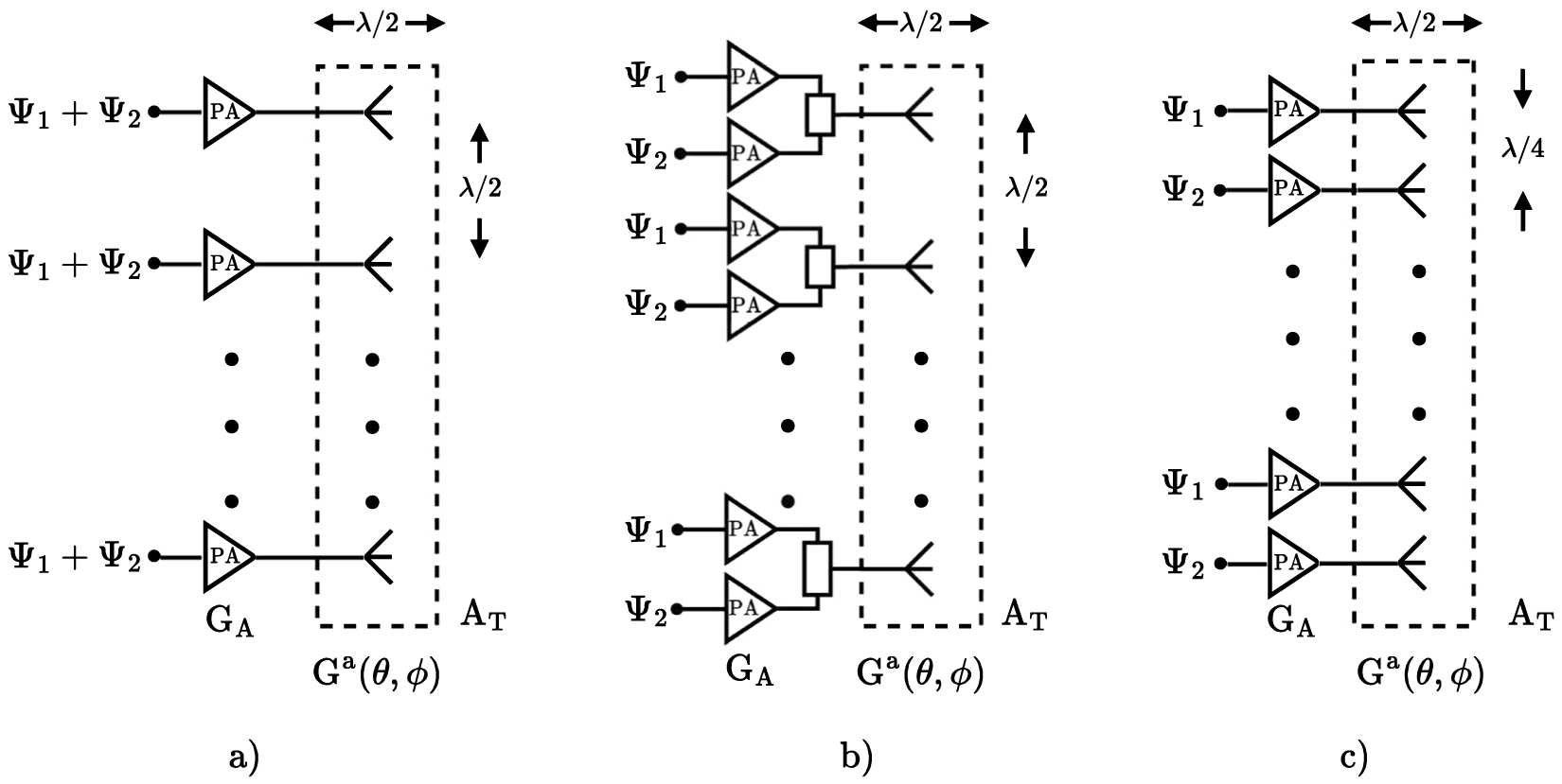


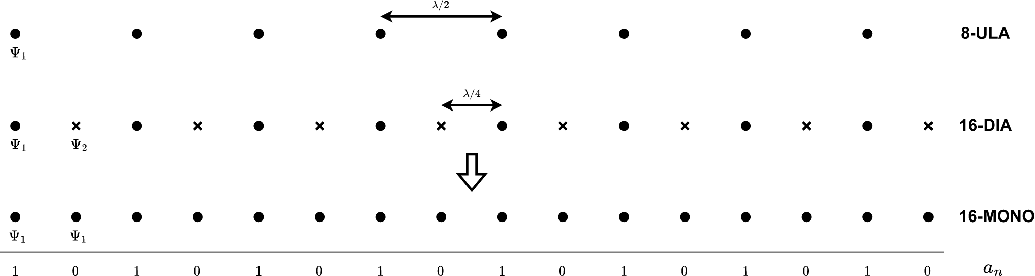


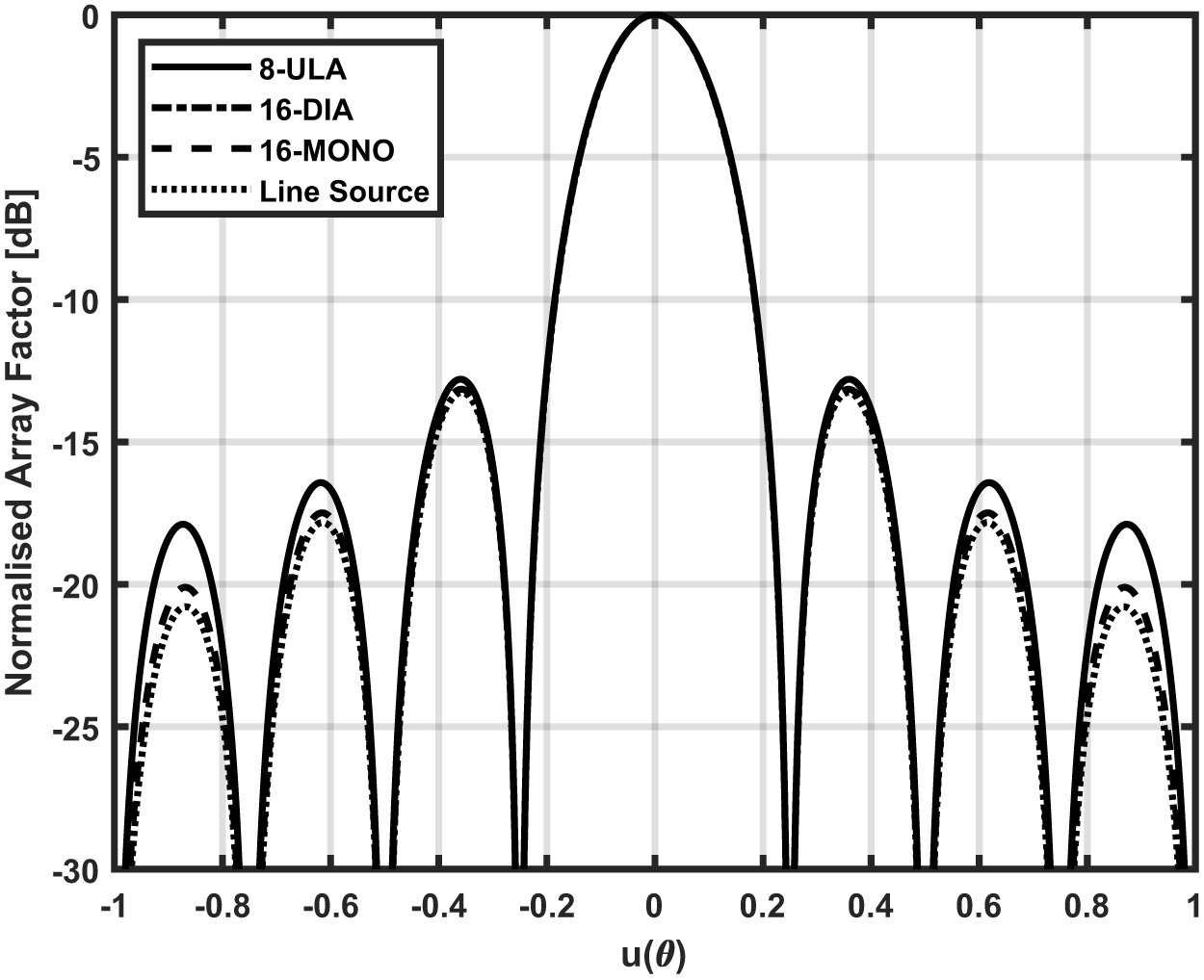


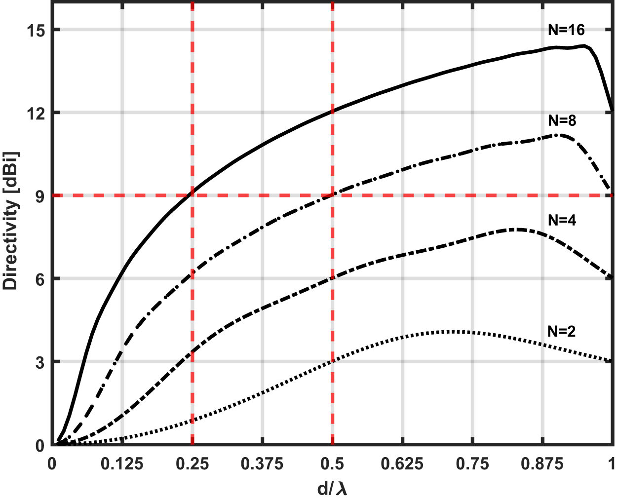
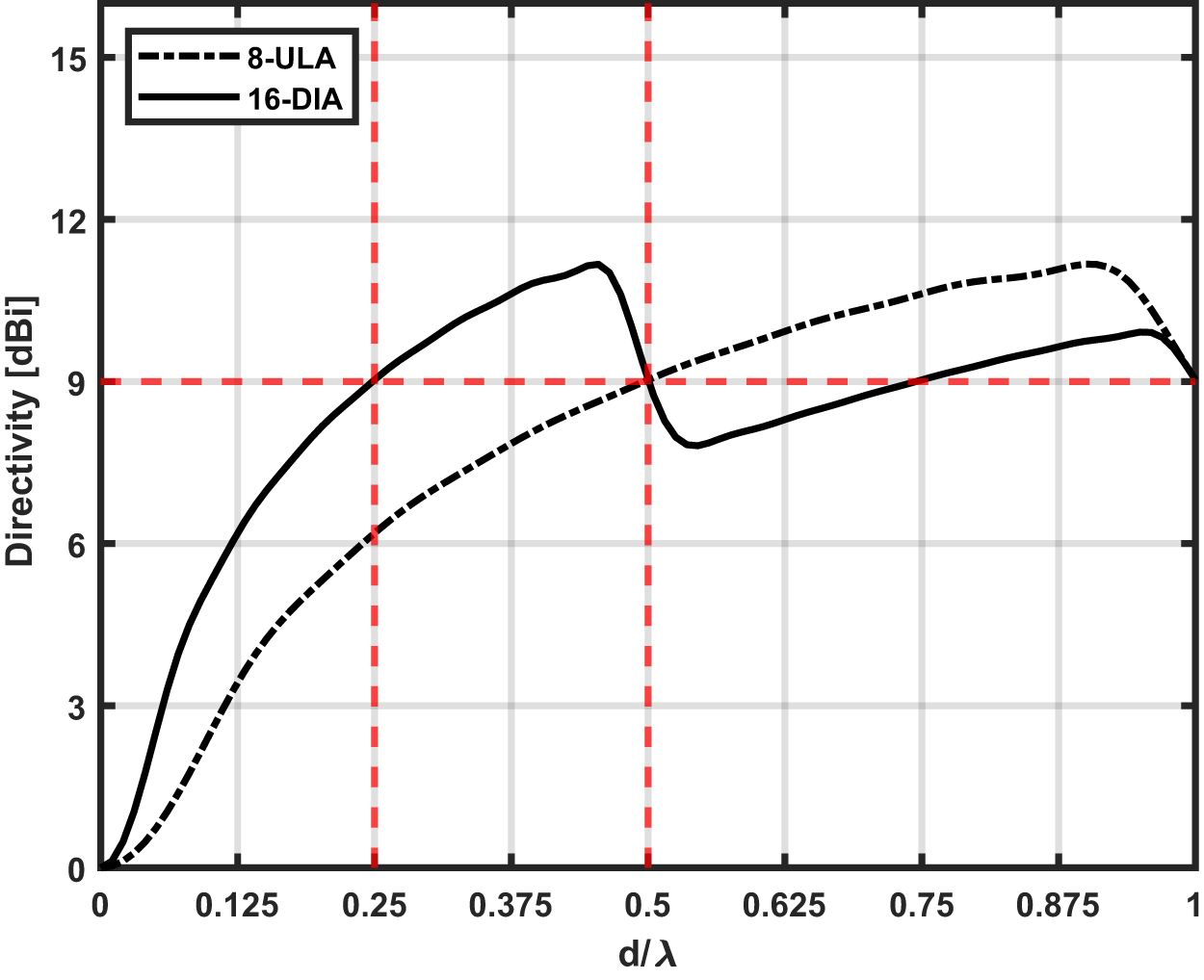


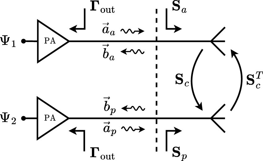

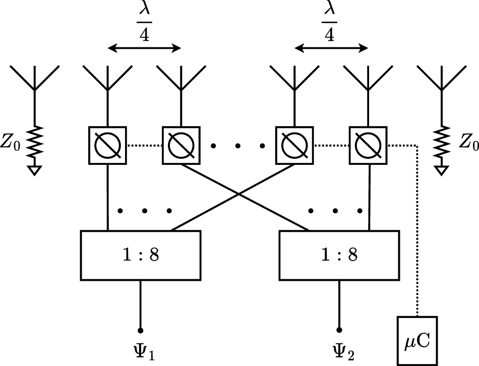


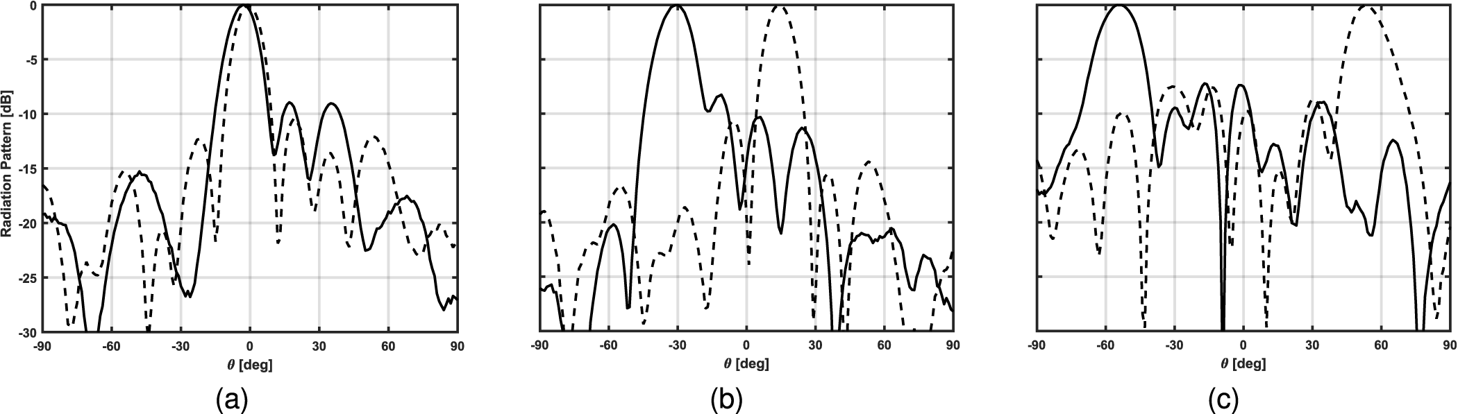


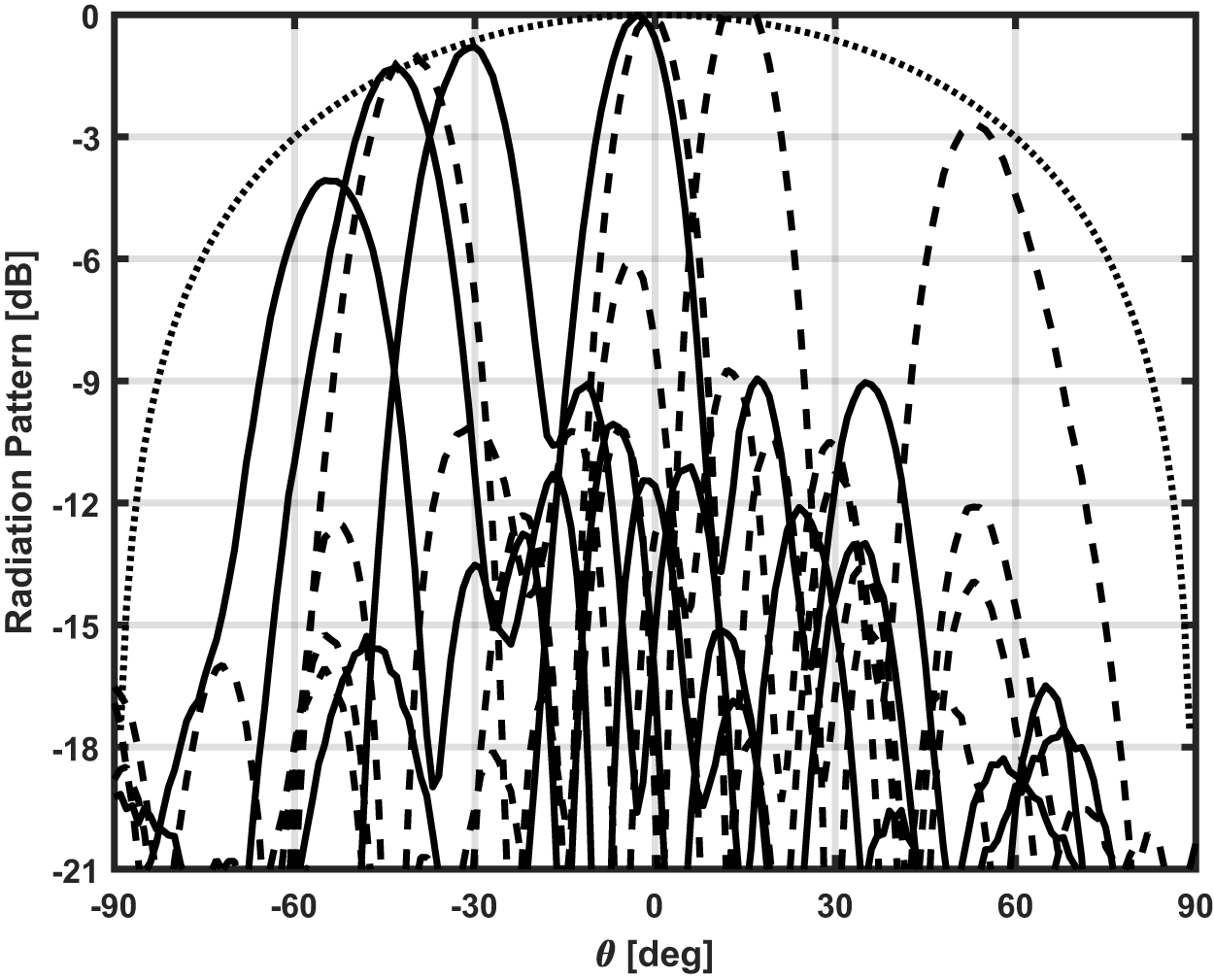


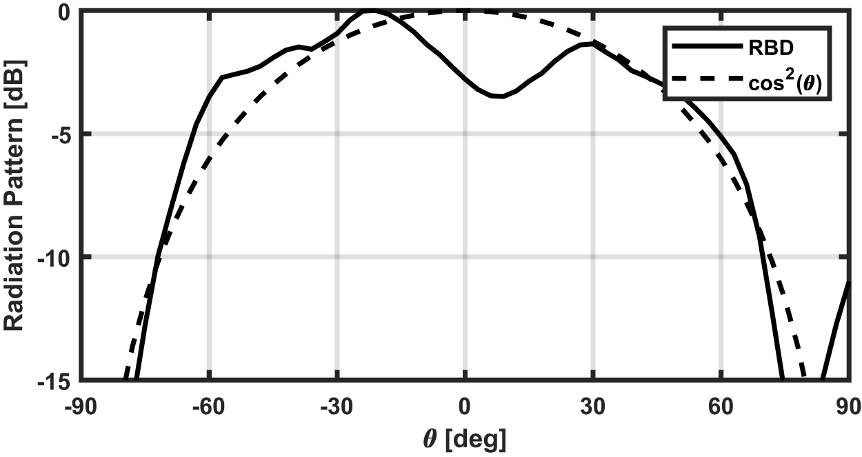


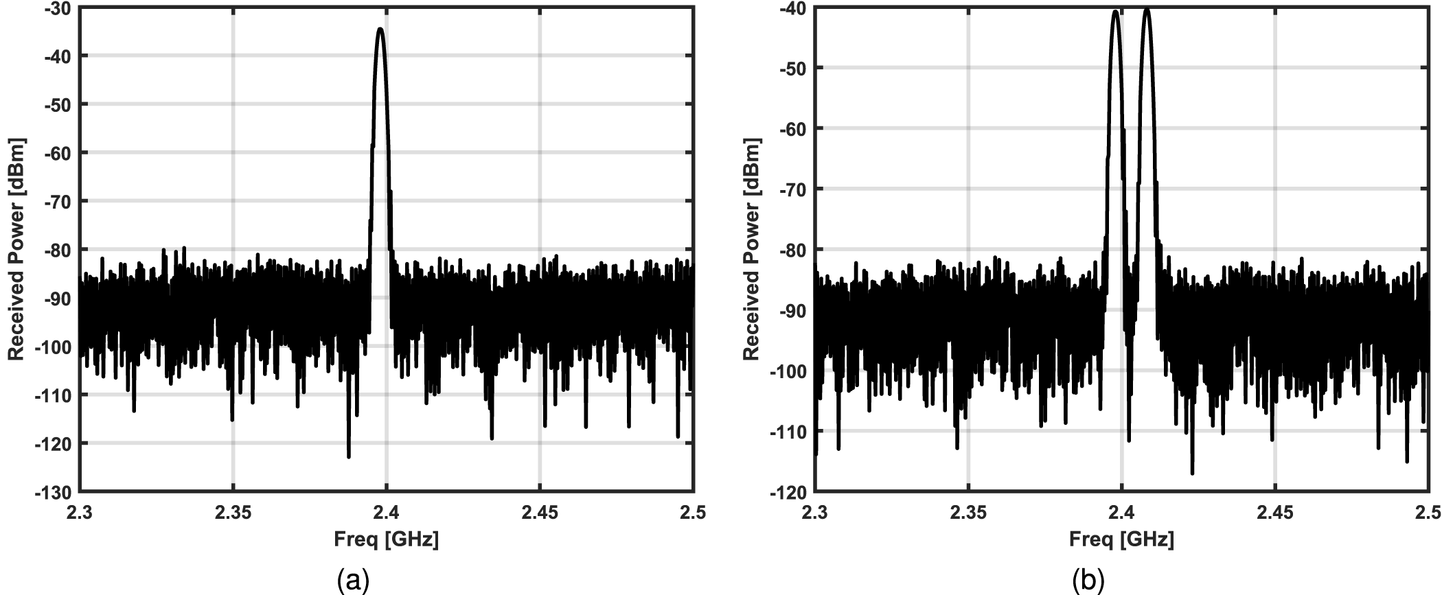


 Open access