


1. Introduction
Microswimmers are particles that can propel themselves in liquids; examples include natural swimming microorganisms and artificial microrobots. Suspensions of microswimmers can be found in a wide range of areas. For example, harmful red tides in the ocean are caused by motile red tide microalgae, which damage the aquaculture industry and affect the environment. The gut flora contains motile bacteria that play an important role in our health. In engineering, swimming microorganisms are utilised in bioreactors for food and water purification. Microrobot technology has also made remarkable progress in recent years, with research into controlling large numbers of microswimmers to perform a task. As transport phenomena in microswimmer suspensions are essential for predicting and controlling the distribution and growth of microswimmers, it is an important area of scientific research.
Although there have been many studies of microswimmer suspensions, not many have carefully considered the hydrodynamics. For example, the simplest active Brownian particle model neglects hydrodynamic, phoretic and essentially all other interactions between active colloids other than steric repulsion. Hydrodynamics becomes particularly important when discussing non-dilute suspensions, because the lubrication flow generates a large force when the swimmers are in close proximity to each other or to a wall boundary. An accurate description of the hydrodynamics allows the near-field interaction of the microswimmers to be properly handled, allowing the analysis of swimming behaviour in concentrated suspensions. In addition, the strong lubrication forces between the microswimmers have a significant influence on the bulk stress field, so that near-field hydrodynamics is crucial for understanding the rheological properties of non-dilute suspensions. Assuming the volume fraction of microswimmers is $\phi$
, the effect of a single swimmer on the stress field is
$\phi$
, the effect of a single swimmer on the stress field is ${\mathcal O} ( \phi )$
, the effect of two-body interaction between swimmers is
${\mathcal O} ( \phi )$
, the effect of two-body interaction between swimmers is ${\mathcal O} ( \phi ^2 )$
and the effect of three-body or more interaction is
${\mathcal O} ( \phi ^2 )$
and the effect of three-body or more interaction is ${\mathcal O} ( \phi ^3 )$
. In the dilute regime, the effects of two-body interactions can be ignored, while in the non-dilute regime, the effects become apparent. In the concentrated regime, three-body or more interactions become apparent. This paper focuses on hydrodynamics and describes the transport phenomena of microswimmer suspensions, such as migration, collective motion, diffusion and rheology.
${\mathcal O} ( \phi ^3 )$
. In the dilute regime, the effects of two-body interactions can be ignored, while in the non-dilute regime, the effects become apparent. In the concentrated regime, three-body or more interactions become apparent. This paper focuses on hydrodynamics and describes the transport phenomena of microswimmer suspensions, such as migration, collective motion, diffusion and rheology.
At the macroscopic continuum level, the transport of microswimmers has been discussed using conservation laws. A conservation law for microswimmers exhibits distinct characteristics as compared with those of passive particles, given that the internal particles are in a state of spontaneous motion. If the spreading of microswimmers is diffusive, a transport equation for the number density of swimmers $n$
can be written as (Pedley & Kessler Reference Pedley and Kessler1992)
$n$
can be written as (Pedley & Kessler Reference Pedley and Kessler1992)
 \begin{equation} \frac {\partial n}{\partial t} = - \boldsymbol{\nabla} {\boldsymbol\cdot} \left [ \left ( \boldsymbol{v} + \langle \boldsymbol{U} \rangle \right ) n - \boldsymbol {D}_t \boldsymbol{\cdot} \boldsymbol{\nabla } n \right ] , \end{equation}
where $\boldsymbol{v}$
is the bulk fluid velocity,
$\boldsymbol{v}$
is the bulk fluid velocity, $\langle \boldsymbol{U} \rangle$
is the average swimming velocity of the microswimmers,
$\langle \boldsymbol{U} \rangle$
is the average swimming velocity of the microswimmers, $\langle \ \rangle$
is the ensemble average and
$\langle \ \rangle$
is the ensemble average and $\boldsymbol {D}_t$
is the translational self-diffusion tensor. If the diffusion phenomenon is isotropic, then the self-diffusivity is a scalar quantity rather than a tensor. The form of this equation is similar to the advection–diffusion equation for passive particles, but with the new appearance of the swimming velocity in the advection term. When the same microswimmers are suspended in a dilute state, the average swimming velocity can be approximated as
$\boldsymbol {D}_t$
is the translational self-diffusion tensor. If the diffusion phenomenon is isotropic, then the self-diffusivity is a scalar quantity rather than a tensor. The form of this equation is similar to the advection–diffusion equation for passive particles, but with the new appearance of the swimming velocity in the advection term. When the same microswimmers are suspended in a dilute state, the average swimming velocity can be approximated as
 \begin{equation} \boldsymbol{U} = U_0 \langle \boldsymbol{p} \rangle , \end{equation}
where $U_0$
is the swimming velocity of a solitary microswimmer in an infinite fluid and
$U_0$
is the swimming velocity of a solitary microswimmer in an infinite fluid and $\boldsymbol{p}$
is the unit orientation vector of a microswimmer. The question here is how to describe the orientation
$\boldsymbol{p}$
is the unit orientation vector of a microswimmer. The question here is how to describe the orientation $\boldsymbol{p}$
. The mathematical description of
$\boldsymbol{p}$
. The mathematical description of $\boldsymbol{p}$
is not straightforward, because microswimmers respond passively or actively to their environment. In non-dilute suspensions, the orientation
$\boldsymbol{p}$
is not straightforward, because microswimmers respond passively or actively to their environment. In non-dilute suspensions, the orientation $\boldsymbol{p}$
changes due to hydrodynamic interactions between microswimmers. Transport of microswimmers may involve adjustment of their orientation, which induces bulk migration of swimmers. Another important question is how to represent the diffusion tensor
$\boldsymbol{p}$
changes due to hydrodynamic interactions between microswimmers. Transport of microswimmers may involve adjustment of their orientation, which induces bulk migration of swimmers. Another important question is how to represent the diffusion tensor $\boldsymbol {D}_t$
, which is strongly affected by the orientation
$\boldsymbol {D}_t$
, which is strongly affected by the orientation $\boldsymbol{p}$
of the microswimmers. In concentrated suspensions, the effect of hydrodynamic interactions on
$\boldsymbol{p}$
of the microswimmers. In concentrated suspensions, the effect of hydrodynamic interactions on $\boldsymbol {D}_t$
is likely to be significant. It is also non-trivial as to whether the spreading of microswimmers can be described as diffusive or not.
$\boldsymbol {D}_t$
is likely to be significant. It is also non-trivial as to whether the spreading of microswimmers can be described as diffusive or not.
In higher-resolution conservation laws of microswimmers, the orientation distribution of microswimmers has been treated explicitly. The probability distribution function (PDF) for a microswimmer located at position $\boldsymbol{x}$
with orientation
$\boldsymbol{x}$
with orientation $\boldsymbol{p}$
at time
$\boldsymbol{p}$
at time $t$
is denoted as
$t$
is denoted as $\Psi (\boldsymbol{x}, \boldsymbol{p}, t)$
. The number density of microswimmers
$\Psi (\boldsymbol{x}, \boldsymbol{p}, t)$
. The number density of microswimmers $n$
is written by using
$n$
is written by using $\Psi$
as
$\Psi$
as
 \begin{equation} n = \int \Psi {\rm d}\boldsymbol{p} , \end{equation}
where the integral is taken over the two-dimensional orientational space. Assuming that the suspension is dilute and that the translational and rotational diffusion are isotropic, the conservation of probability can be written as (Lauga Reference Lauga2020)
 \begin{equation} \frac {\partial \Psi }{\partial t} = - \boldsymbol{\nabla } \boldsymbol{\cdot} [( \boldsymbol{u} + U_0 \boldsymbol{p}) \Psi - D_t \boldsymbol{\nabla } \Psi] - \boldsymbol{\nabla }_{\! p} \boldsymbol{\cdot} [\dot {\boldsymbol{p}} \, \Psi - D_r \boldsymbol{\nabla }_{\! p}\Psi], \end{equation}
where $D_r$
is the rotational diffusivity,
$D_r$
is the rotational diffusivity, $\boldsymbol{\nabla }_{\! p}$
is the gradient on the unit sphere and
$\boldsymbol{\nabla }_{\! p}$
is the gradient on the unit sphere and $\dot {\boldsymbol{p}}$
is the rate of change in the microswimmer orientation. The mathematical description of
$\dot {\boldsymbol{p}}$
is the rate of change in the microswimmer orientation. The mathematical description of $\dot {\boldsymbol{p}}$
is again not straightforward, because it is influenced by the response of the swimmers to their environment and the hydrodynamic interactions between the swimmers. A non-zero
$\dot {\boldsymbol{p}}$
is again not straightforward, because it is influenced by the response of the swimmers to their environment and the hydrodynamic interactions between the swimmers. A non-zero $\langle \boldsymbol{p} \rangle$
induces migration of microswimmers, which is described in § 3. If the suspension is non-dilute, the interactions between the microswimmers can induce collective motions, such as coherent structures, swirls, polar order and clustering. The collective motions affect not only the orientation
$\langle \boldsymbol{p} \rangle$
induces migration of microswimmers, which is described in § 3. If the suspension is non-dilute, the interactions between the microswimmers can induce collective motions, such as coherent structures, swirls, polar order and clustering. The collective motions affect not only the orientation $\boldsymbol{p}$
but also the swimming velocity, which is addressed in § 4. Furthermore, it is again non-trivial as to whether the translational and rotational spreadings of the microswimmers are diffusive or not, and even if they are diffusive, whether they are isotropic or not. We discuss the self-diffusion of microswimmers in § 5.1.
$\boldsymbol{p}$
but also the swimming velocity, which is addressed in § 4. Furthermore, it is again non-trivial as to whether the translational and rotational spreadings of the microswimmers are diffusive or not, and even if they are diffusive, whether they are isotropic or not. We discuss the self-diffusion of microswimmers in § 5.1.
Similarly, a transport equation for tracer particles, such as chemical substances and fluid particles, can be written as
 \begin{equation} \frac {\partial c}{\partial t} = - \boldsymbol{\nabla } \boldsymbol{\cdot} [ \boldsymbol{v} c - \boldsymbol {D}_c \boldsymbol{\cdot} \boldsymbol{\nabla } c ] , \end{equation}
where $c$
is the concentration of tracer particles and
$c$
is the concentration of tracer particles and $\boldsymbol {D}_c$
is the diffusion tensor of the tracers. In a suspension of microswimmers, the swimming motion induces a flow of the surrounding fluid, which mixes the surrounding fluid. The diffusion coefficient of the tracers therefore tends to be higher than in passive particle suspensions. In a concentrated suspension of bacteria, the bacteria swim collectively, creating spontaneous vortex structures known as bacterial turbulence. Such chaotic flows dramatically increase the diffusion of the tracer particles. We describe the diffusion of tracers in § 5.2.
$\boldsymbol {D}_c$
is the diffusion tensor of the tracers. In a suspension of microswimmers, the swimming motion induces a flow of the surrounding fluid, which mixes the surrounding fluid. The diffusion coefficient of the tracers therefore tends to be higher than in passive particle suspensions. In a concentrated suspension of bacteria, the bacteria swim collectively, creating spontaneous vortex structures known as bacterial turbulence. Such chaotic flows dramatically increase the diffusion of the tracer particles. We describe the diffusion of tracers in § 5.2.
The momentum transport in the suspension is also influenced by the presence of microswimmers. The bulk stress tensor $\boldsymbol{\Sigma }$
of a microswimmer suspension can be expressed as the sum of the hydrodynamic stress from the background flow and the deviatoric particle stress as
$\boldsymbol{\Sigma }$
of a microswimmer suspension can be expressed as the sum of the hydrodynamic stress from the background flow and the deviatoric particle stress as
 \begin{equation} {\boldsymbol{\Sigma }} = - P {\kern-0.8pt}\boldsymbol {I} + 2 \mu \boldsymbol {E} + {\boldsymbol{\Sigma }}^p , \end{equation}
where $P$
is the pressure,
$P$
is the pressure, $\boldsymbol {I}$
is the unit tensor,
$\boldsymbol {I}$
is the unit tensor, $\mu$
is the viscosity and
$\mu$
is the viscosity and $\boldsymbol {E}$
is the bulk rate of strain tensor. Here
$\boldsymbol {E}$
is the bulk rate of strain tensor. Here ${\boldsymbol{\Sigma }}^p$
is the particle stress tensor expressing the effect of microswimmers. The viscosity of microswimmer suspensions can be higher or lower depending on the characteristics and orientation of the microswimmers. Microswimmer suspensions also exhibit non-Newtonian properties, such as normal stress differences and relaxation time. In concentrated suspensions, the lubrication forces between the microswimmers have a significant influence on the bulk stress field, although this aspect has not been explored in depth. The rheological properties of microswimmer suspensions are discussed in § 6.
${\boldsymbol{\Sigma }}^p$
is the particle stress tensor expressing the effect of microswimmers. The viscosity of microswimmer suspensions can be higher or lower depending on the characteristics and orientation of the microswimmers. Microswimmer suspensions also exhibit non-Newtonian properties, such as normal stress differences and relaxation time. In concentrated suspensions, the lubrication forces between the microswimmers have a significant influence on the bulk stress field, although this aspect has not been explored in depth. The rheological properties of microswimmer suspensions are discussed in § 6.
Whilst previous studies have revealed transport phenomena in the dilute regime, those in the non-dilute to concentrated regime remain largely unexplored. The primary reason for this is that the interaction between microswimmers must be considered when dilution cannot be assumed. The near-field hydrodynamic interactions make mathematical treatment difficult, and the lubrication flow between near-contact surfaces makes numerical treatment difficult. Furthermore, the near-field interactions between microswimmers manifest in a variety of forms, involving not only the flow field, but also the concentration field, electric field, biological responses, etc. This paper focuses on hydrodynamic interactions among them.
This paper is structured to progressively scale up from a single microswimmer to a collective movement to a macroscale continuum. At each scale, the discussion also evolves from dilute to concentrated suspensions. To begin with, in § 2, we introduce natural swimming microorganisms, artificial microswimmers and mathematical models, which will appear in later sections. In addition, the basics of fluid mechanics that are necessary for reading this paper are explained. Section 3 describes the effects of gravity, flow fields and wall boundaries on the migration of microswimmers. Collective swimming, created spontaneously by hydrodynamic interactions between microswimmers, is discussed in § 4. Macroscopic diffusion properties are addressed in § 5.1 for microswimmers and in § 5.2 for tracers. Section 6 describes the rheological properties of microswimmer suspensions in shear flow and Poiseuille flow. Microrheology is also discussed in that section. Finally, in § 7, current issues and future research prospects are discussed.
It should be noted that this paper, being in the category of JFM Perspectives, is not a complete review, but rather a survey from the author’s point of view. This may have biased the selection of some topics, and it is inevitable that some relevant studies have not been properly discussed. To compensate for this, a number of relevant review papers have been cited in each section. If more detailed explanations or associated papers are required, the reader is referred to them. The paper is also structured so that a reader entering the field without specialist knowledge can access and understand the key findings.
2. Microswimmer
2.1. Swimming microorganisms
The diversity of microorganisms and their swimming strategies is so extensive that it is impossible to cover them all in this paper. In the study of microbial suspensions, however, the number of model microorganisms is limited and this section focuses on them. Many swimming microorganisms use cell organelles such as flagella and cilia to propel themselves in liquids. Here, we describe typical swimming strategies of microorganisms using (i) prokaryotic flagella, (ii) eukaryotic flagella and (iii) eukaryotic cilia. The model microorganisms described here are also discussed in subsequent sections.
Escherichia coli is one of the most commonly used model organisms among bacteria (Berg Reference Berg2004). E. coli have helical flagella, as shown in figure 1(a), and propel themselves by rotating them. Prokaryotic flagella are rather rigid and do not actively deform like eukaryotic flagella. The cell body of E. coli is about 1 $\unicode{x03BC}$
m in diameter and 2
$\unicode{x03BC}$
m in diameter and 2 $\unicode{x03BC}$
m in length and swims at a speed of about 20
$\unicode{x03BC}$
m in length and swims at a speed of about 20 $\unicode{x03BC}$
m s–1. This may seem like a slow speed, but 10 times the body length per second can be considered quite fast compared with our swimming speed. Each flagellar filament is attached to a short flexible hook that acts as a universal joint and is connected to a rotary motor embedded in the cell wall. When all of the motors rotate in the counterclockwise direction, the flagella generate a flow to form a flagellar bundle. The flagellar bundle behaves like a corkscrew and propels the cell body by rotation. There is no external torque acting on the cells, so they are torque-free during swimming. As the rotation of the flagella produces a torque, a counteracting torque is produced in the bacterial body. Therefore, the flagella and the cell body rotate in opposite directions during swimming.
$\unicode{x03BC}$
m s–1. This may seem like a slow speed, but 10 times the body length per second can be considered quite fast compared with our swimming speed. Each flagellar filament is attached to a short flexible hook that acts as a universal joint and is connected to a rotary motor embedded in the cell wall. When all of the motors rotate in the counterclockwise direction, the flagella generate a flow to form a flagellar bundle. The flagellar bundle behaves like a corkscrew and propels the cell body by rotation. There is no external torque acting on the cells, so they are torque-free during swimming. As the rotation of the flagella produces a torque, a counteracting torque is produced in the bacterial body. Therefore, the flagella and the cell body rotate in opposite directions during swimming.
Swimming microorganisms. (a) Escherichia coli bacterium. Reproduced from Turner, Ryu & Berg (Reference Turner, Ryu and Berg2000) with permission. Copyright $\unicode{x00A9}$
2000 American Society for Microbiology. (b) Two Bacillus subtilis bacteria about to separate after cell division. Reproduced from Cisneros et al. (Reference Cisneros, Cortez, Dombrowski, Goldstein and Kessler2007) with permission. Copyright
$\unicode{x00A9}$
2007 Springer-Verlag. (c) Human spermatozoon swimming in high-viscosity liquid. Reproduced from Smith et al. (Reference Smith, Gaffney, Gadêlha, Kapur and Kirkman-Brown2009) with permission. Copyright
$\unicode{x00A9}$
2009 Wiley-Liss, Inc. (d) Flagellar waveform of a microalga Chlamydomonas reinhardtii. Reproduced from Leptos et al. (Reference Leptos, Chioccioli, Furlan, Pesci and Goldstein2023). CC BY 4.0. (e) Microalga Volvox carteri. Reproduced from Russell et al. (Reference Russell2017). CC BY 4.0. ( f) Ciliate Tetrahymena thermophila, where OA indicates the oral apparatus. Reproduced from Soares et al. (Reference Soares, Carmona, Nolasco and Viseu2019). CC BY 4.0. (g) Ciliate Paramecium caudatum. Reproduced from Hausmann & Allen (Reference Hausmann and Allen2010) with permission. Copyright
$\unicode{x00A9}$
2010 Elsevier Inc.
$\unicode{x00A9}$
2000 American Society for Microbiology. (b) Two Bacillus subtilis bacteria about to separate after cell division. Reproduced from Cisneros et al. (Reference Cisneros, Cortez, Dombrowski, Goldstein and Kessler2007) with permission. Copyright
$\unicode{x00A9}$
2007 Springer-Verlag. (c) Human spermatozoon swimming in high-viscosity liquid. Reproduced from Smith et al. (Reference Smith, Gaffney, Gadêlha, Kapur and Kirkman-Brown2009) with permission. Copyright
$\unicode{x00A9}$
2009 Wiley-Liss, Inc. (d) Flagellar waveform of a microalga Chlamydomonas reinhardtii. Reproduced from Leptos et al. (Reference Leptos, Chioccioli, Furlan, Pesci and Goldstein2023). CC BY 4.0. (e) Microalga Volvox carteri. Reproduced from Russell et al. (Reference Russell2017). CC BY 4.0. ( f) Ciliate Tetrahymena thermophila, where OA indicates the oral apparatus. Reproduced from Soares et al. (Reference Soares, Carmona, Nolasco and Viseu2019). CC BY 4.0. (g) Ciliate Paramecium caudatum. Reproduced from Hausmann & Allen (Reference Hausmann and Allen2010) with permission. Copyright
$\unicode{x00A9}$
2010 Elsevier Inc.

Bacillus subtilis is a commonly used model bacterium alongside E. coli. B. subtilis is on average about 4 $\unicode{x03BC}$
m long, with about 20 flagella growing peritrichously (uniformly) around the cell, as shown in figure 1(b). B. subtilis, like E. coli, swims with multiple flagella in bundles and has a swimming speed of about 20
$\unicode{x03BC}$
m long, with about 20 flagella growing peritrichously (uniformly) around the cell, as shown in figure 1(b). B. subtilis, like E. coli, swims with multiple flagella in bundles and has a swimming speed of about 20 $\unicode{x03BC}$
m s–1 (Najafi et al. Reference Najafi, Altegoer, Bange and Wagner2019). The swimming is interrupted by tumbles in which the direction of flagellar rotation is briefly reversed, resulting in a change of orientation. B. subtilis uses a biased random walk strategy for chemotaxis, i.e. swimming towards an attractant. Similar chemotactic behaviour has been well studied in E. coli.
$\unicode{x03BC}$
m s–1 (Najafi et al. Reference Najafi, Altegoer, Bange and Wagner2019). The swimming is interrupted by tumbles in which the direction of flagellar rotation is briefly reversed, resulting in a change of orientation. B. subtilis uses a biased random walk strategy for chemotaxis, i.e. swimming towards an attractant. Similar chemotactic behaviour has been well studied in E. coli.
Eukaryotic flagella are shaped like long hairs, similar to prokaryotic flagella, but their structure and movement are very different. The structure of a eukaryotic flagellum has ninefold symmetry with nine outer doublet microtubules and two central pairs of microtubules, known as the $9+2$
structure. This structure is conserved in most eukaryotic organisms. Dynein molecular motors are equally spaced on each outer doublet microtubule, creating a sliding force between the microtubules along the entire flagellum, resulting in a periodic flagellar waveform. Sperm motility is an important medical and biological phenomenon that has been extensively studied (Gaffney et al. Reference Gaffney, Gadêlha, Smith, Blake and Kirkman-Brown2011). Human spermatozoa have a head length of 5
$9+2$
structure. This structure is conserved in most eukaryotic organisms. Dynein molecular motors are equally spaced on each outer doublet microtubule, creating a sliding force between the microtubules along the entire flagellum, resulting in a periodic flagellar waveform. Sperm motility is an important medical and biological phenomenon that has been extensively studied (Gaffney et al. Reference Gaffney, Gadêlha, Smith, Blake and Kirkman-Brown2011). Human spermatozoa have a head length of 5 $\unicode{x03BC}$
m and a flagellum length of about 55
$\unicode{x03BC}$
m and a flagellum length of about 55 $\unicode{x03BC}$
m. The flagellum beats like a whip to form a wave propagating from the head to the tail, as shown in figure 1(c). The sperm swims in the opposite direction to the wave propagation direction of the flagellum. Although its motility varies with physiological state and the surrounding physicochemical environment, it swims at a speed of approximately
$\unicode{x03BC}$
m. The flagellum beats like a whip to form a wave propagating from the head to the tail, as shown in figure 1(c). The sperm swims in the opposite direction to the wave propagation direction of the flagellum. Although its motility varies with physiological state and the surrounding physicochemical environment, it swims at a speed of approximately $30{-}50$
μm s–1.
$30{-}50$
μm s–1.
Microalgae are eukaryotic, unicellular microorganisms that are photosynthetic and typically have an aquatic lifestyle (Thoré et al. Reference Thoré, Muylaert, Bertram and Brodin2023). Microalgae are the main primary producers in ecosystems, providing energy and organic matter for zooplankton and fish. In industry, microalgae are produced commercially for the production of biofuels and nutritional supplements. In the field of fluid mechanics, Chlamydomonas reinhardtii is one of the most commonly used model organisms among microalgae. The body length of C. reinhardtii is $7{-}10\,\unicode{x03BC}$
m, and the organism is equipped with two
$7{-}10\,\unicode{x03BC}$
m, and the organism is equipped with two $10 {-} 12\,\unicode{x03BC}$
m long flagella on its anterior side. The flagella oscillate at
$10 {-} 12\,\unicode{x03BC}$
m long flagella on its anterior side. The flagella oscillate at $50 {-} 60$
Hz and repeat effective strokes, which produce a large thrust, and recovery strokes, which produce resistance, as shown in figure 1(d). The cell moves forward during the effective strokes and backward during the recovery strokes, swimming at a time average speed of
$50 {-} 60$
Hz and repeat effective strokes, which produce a large thrust, and recovery strokes, which produce resistance, as shown in figure 1(d). The cell moves forward during the effective strokes and backward during the recovery strokes, swimming at a time average speed of $100{-}200\,\unicode{x03BC}$
m s–1.
$100{-}200\,\unicode{x03BC}$
m s–1.
Eukaryotic cilia have the same structure as eukaryotic flagella, but cilia are short and numerous, whereas flagella are long and few. Among the microorganisms that swim with cilia, Volvox has been the subject of much hydrodynamic research because of its spherical shape, which makes it easier to handle mathematically (Goldstein Reference Goldstein2015; Pedley Reference Pedley2016). Volvox carteri, shown in figure 1(e), has a spherical colony consisting of about 2000 somatic cells on the outside and a number of germ cells on the inside (Kirk Reference Kirk2008). The colony is covered by approximately 4000 cilia that move together in a synchronised manner, creating a metacronal wave on the colony surface. Each somatic cell has two flagella, and these all beat more or less in planes that are offset from the purely meridional planes by an angle of $10^\circ{-}20^\circ$
(Pedley Reference Pedley2016). This offset causes the spinning motion of Volvox as it swims.
$10^\circ{-}20^\circ$
(Pedley Reference Pedley2016). This offset causes the spinning motion of Volvox as it swims.
One of the most prevalent microorganisms that utilise cilia for locomotion is the ciliate. Tetrahymena thermophila, shown in figure 1(f), has been employed as a model organism in the fields of fluid mechanics, molecular biology and cellular biology. The body length and width of T. thermophila are approximately 50 and 30 $\unicode{x03BC}$
m, respectively. The cell body is covered by approximately 750 cilia (Soares et al. Reference Soares, Carmona, Nolasco and Viseu2019), of which about 150 are oral cilia, organised into membranelles that sweep food particles into the oral cavity. Each cilium undergoes effective and recovery strokes, and the swimming speed is approximately
$\unicode{x03BC}$
m, respectively. The cell body is covered by approximately 750 cilia (Soares et al. Reference Soares, Carmona, Nolasco and Viseu2019), of which about 150 are oral cilia, organised into membranelles that sweep food particles into the oral cavity. Each cilium undergoes effective and recovery strokes, and the swimming speed is approximately $400{-}500\,\unicode{x03BC}$
m s–1. Another model ciliate used in the field of fluid mechanics is Paramecium caudatum. The body length and width of P. caudatum, shown in figure 1(g), are about 250 and 50
$400{-}500\,\unicode{x03BC}$
m s–1. Another model ciliate used in the field of fluid mechanics is Paramecium caudatum. The body length and width of P. caudatum, shown in figure 1(g), are about 250 and 50 $\unicode{x03BC}$
m, respectively. Approximately 15 000 cilia are distributed over the entire body of an individual organism, with a density of about 50 cilia per 100
$\unicode{x03BC}$
m, respectively. Approximately 15 000 cilia are distributed over the entire body of an individual organism, with a density of about 50 cilia per 100 $\unicode{x03BC}$
m
$\unicode{x03BC}$
m $^2$
(Brennen & Winet Reference Brennen and Winet1977). The cilia are about 10–15
$^2$
(Brennen & Winet Reference Brennen and Winet1977). The cilia are about 10–15 $\unicode{x03BC}$
m in length and 0.2
$\unicode{x03BC}$
m in length and 0.2 $\unicode{x03BC}$
m in diameter. The cilia beat at a frequency of about 30 Hz, and P. caudatum swims at about 10 body lengths per second.
$\unicode{x03BC}$
m in diameter. The cilia beat at a frequency of about 30 Hz, and P. caudatum swims at about 10 body lengths per second.
2.2. Artificial and model microswimmers
Various artificial microswimmers have been developed, powered by a variety of driving principles, such as magnetic, electric and concentration fields, light, heat and sound waves (Tsang et al. Reference Tsang, Demir, Ding and Pak2020; Wu et al. Reference Wu, Chen, Mukasa, Pak and Gao2020). A number of mathematical models have also been developed to analyse various microswimmers. As it is not possible to give an exhaustive description of all of them in this section, the artificial microswimmers and mathematical models that appear in the following sections are described.
Artificial and model microswimmers. (a) Schematic illustration of self-diffusiophoresis due to neutral solute gradients with one reactant (blue) and one product (yellow). The swimmer is a colloidal Janus sphere with inert (light grey) and catalytic (dark grey) hemispheres. A phoretic fluid flow occurs from the inert to the catalytic side of the swimmer, and the Janus sphere moves from right to left as shown by the yellow arrow. Reproduced from Moran & Posner (Reference Moran and Posner2017) with permission. Copyright
$\unicode{x00A9}$
2017 Annual Reviews. (b) Streamlines around solitary squirmers in the body frame (i–iii) and laboratory frame (iv–vi). (i,iv) Pusher with a negative stresslet ( $\beta = -5$
). (ii,v) Neutral squirmer with
$\beta = -5$
). (ii,v) Neutral squirmer with $\beta = 0$
. (iii,vi) Puller with a positive stresslet (
$\beta = 0$
. (iii,vi) Puller with a positive stresslet ( $\beta = 5$
). Reproduced from Evans et al. (Reference Evans, Ishikawa, Yamaguchi and Lauga2011) with permission. Copyright
$\unicode{x00A9}$
2011 American Institute of Physics. (c) Active Brownian particles of radius
$\beta = 5$
). Reproduced from Evans et al. (Reference Evans, Ishikawa, Yamaguchi and Lauga2011) with permission. Copyright
$\unicode{x00A9}$
2011 American Institute of Physics. (c) Active Brownian particles of radius $1\,\unicode{x03BC}$
m moving in two dimensions in a water environment. (i) An ABP propels itself with speed
$1\,\unicode{x03BC}$
m moving in two dimensions in a water environment. (i) An ABP propels itself with speed $U_0$
while undergoing Brownian motion in both position and orientation. The resulting trajectories are shown for different velocities: (ii)
$U_0$
while undergoing Brownian motion in both position and orientation. The resulting trajectories are shown for different velocities: (ii) $U_0 = 0\,\unicode{x03BC}$
m s–1 (Brownian particle), (iii)
$U_0 = 0\,\unicode{x03BC}$
m s–1 (Brownian particle), (iii) $U_0 = 1\,\unicode{x03BC}$
m s–1, (iv)
$U_0 = 1\,\unicode{x03BC}$
m s–1, (iv) $U_0 = 2\,\unicode{x03BC}$
m s–1 and (v)
$U_0 = 2\,\unicode{x03BC}$
m s–1 and (v) $U_0 = 3\,\unicode{x03BC}$
m s–1. Reproduced from Bechinger et al. (Reference Bechinger, Di Leonardo, Löwen, Reichhardt, Volpe and Volpe2016) with permission. Copyright
$\unicode{x00A9}$
2016 American Physical Society.
$U_0 = 3\,\unicode{x03BC}$
m s–1. Reproduced from Bechinger et al. (Reference Bechinger, Di Leonardo, Löwen, Reichhardt, Volpe and Volpe2016) with permission. Copyright
$\unicode{x00A9}$
2016 American Physical Society.

Phoretic self-propulsion is one of the most prevalent swimming mechanisms employed in the field of artificial microswimmers. Phoretic self-propulsion utilises gradients of solute concentration, electric potential or temperature to generate flow in the vicinity of the swimmer surface. If the swimmer itself is capable of generating these gradients, such as through surface chemical reactions or by emitting or absorbing heat, phoretic effects can generate self-propelled motion (Moran & Posner Reference Moran and Posner2017). Figure 2(a) is a schematic illustration of self-diffusiophoresis due to neutral solute gradients with one reactant (blue) and one product (yellow). The swimmer is a colloidal Janus sphere with inert (light grey) and catalytic (dark grey) hemispheres. In this configuration, the catalytic half facilitates the conversion of a single reactant particle into two product particles upon contact with the catalytic surface. A phoretic fluid flow occurs from the inert to the catalytic side of the swimmer, and the Janus sphere moves from right to left as shown by a yellow arrow. In the mathematical analysis of phoretic microswimmers, the fluid domain is often split into two regions: the bulk and the interfacial region around the particle (Moran & Posner Reference Moran and Posner2017). Under the assumption that phoretic effects are confined to the thin interfacial region, such effects can be represented as surface slip velocities. In this case, a phoretic microswimmer can be modelled as a squirmer, which is discussed later in this section. However, such a simplified assumption may not be applicable in cases where multiple phoretic microswimmers interact with each other. This is because each swimmer changes the distribution of the product (or reactant) solute, which in turn changes the motion of the other swimmers. Therefore, a concentration field as well as a flow field have to be solved simultaneously.
Microscale active droplets are able to swim autonomously. Michelin (Reference Michelin2023) classified chemically active droplets into two principal categories: (i) reacting droplets and (ii) solubilising droplets. The former category of droplets typically uses chemical reactions to alter the structure of surfactant molecules at their interface, thereby modifying their tensio-active properties. In contrast, the latter mechanism relies on the dissolution of micelles into a surfactant-saturated environment. Both mechanisms affect the surface tension of the droplet, triggering self-induced Marangoni flows. When velocity is generated at the droplet surface, flow is also generated in the surrounding fluid, allowing the droplet to migrate.
A microswimmer model with prescribed surface velocity is called a squirmer (Lighthill Reference Lighthill1952; Blake Reference Blake1971; Pedley Reference Pedley2016). The surface velocity for an axisymmetric, nearly spherical squirmer can be generally expressed as
 \begin{equation} u_r=\sum _{n=0}^\infty A_n(t) P_n (\cos \theta ),\qquad u_\theta = \sum _{n=1}^\infty B_n(t)V_n(\cos \theta ), \end{equation}
where $P_n$
is the
$P_n$
is the $n{\rm th}$
Legendre polynomial and
$n{\rm th}$
Legendre polynomial and $V_n$
is defined as
$V_n$
is defined as
 \begin{equation} V_n (\cos \theta )=\frac {2}{n(n+1)}\sin \theta \, P_n^\prime (\cos \theta ). \end{equation}
Velocities $u_r$
and
$u_r$
and $u_\theta$
are the velocities in the
$u_\theta$
are the velocities in the $r$
and
$r$
and $\theta$
directions in spherical polar coordinates. The spherical coordinates are defined such that
$\theta$
directions in spherical polar coordinates. The spherical coordinates are defined such that $\theta =0$
and
$\theta =0$
and $\theta =\pi$
denote the axis of axisymmetry, and
$\theta =\pi$
denote the axis of axisymmetry, and $\theta =0$
indicates the swimming direction
$\theta =0$
indicates the swimming direction $\boldsymbol{p}$
. Coefficients
$\boldsymbol{p}$
. Coefficients $A_n(t)$
and
$A_n(t)$
and $B_n(t)$
are the time-dependent coefficients of each squirming mode. In many studies, the radial velocity is assumed to be zero and the tangential velocity is assumed to be invariant with time, i.e. a steady spherical squirmer. In this case, the swimming velocity of a solitary squirmer in a fluid otherwise at rest is
$B_n(t)$
are the time-dependent coefficients of each squirming mode. In many studies, the radial velocity is assumed to be zero and the tangential velocity is assumed to be invariant with time, i.e. a steady spherical squirmer. In this case, the swimming velocity of a solitary squirmer in a fluid otherwise at rest is $U_0 = 2 B_1 / 3$
, and the contribution of the solitary squirmer to the stress field, such as viscosity, is governed only by
$U_0 = 2 B_1 / 3$
, and the contribution of the solitary squirmer to the stress field, such as viscosity, is governed only by $B_2$
. Therefore, further simplified models that only consider the first two modes are often used. The surface velocity of this most simplified squirmer model is given by
$B_2$
. Therefore, further simplified models that only consider the first two modes are often used. The surface velocity of this most simplified squirmer model is given by
 \begin{equation} u_r = 0,\qquad u_\theta = \frac {3 U_0}{2} \left ( \sin {\theta } + \beta \sin {\theta } \cos {\theta } \right )\!, \end{equation}
where $\beta$
is the squirmer parameter indicating the ratio of the second-mode to the first-mode squirming
$\beta$
is the squirmer parameter indicating the ratio of the second-mode to the first-mode squirming $(\beta = B_2 / B_1)$
. A squirmer with a positive
$(\beta = B_2 / B_1)$
. A squirmer with a positive $\beta$
is a puller, generating thrust in front of the body, while a squirmer with a negative
$\beta$
is a puller, generating thrust in front of the body, while a squirmer with a negative $\beta$
is a pusher, generating thrust behind the body. A squirmer with
$\beta$
is a pusher, generating thrust behind the body. A squirmer with $\beta = 0$
is a neutral swimmer. The velocity fields around the puller, pusher and neutral squirmers are shown in figure 2(b).
$\beta = 0$
is a neutral swimmer. The velocity fields around the puller, pusher and neutral squirmers are shown in figure 2(b).
Mathematical models of active colloids are reviewed by Zöttl & Stark (Reference Zöttl and Stark2023). One of the simplest models to describe the behaviour of active colloids is the active Brownian particle (ABP) model. The simplest ABP model neglects hydrodynamic, phoretic and essentially all other interactions between active colloids other than steric repulsion. The ABP model has an intrinsic speed $U_0$
in the direction
$U_0$
in the direction $\boldsymbol{p}(t)$
, under the influence of translational and rotational Brownian motion. The position
$\boldsymbol{p}(t)$
, under the influence of translational and rotational Brownian motion. The position $\boldsymbol{r}(t)$
and orientation
$\boldsymbol{r}(t)$
and orientation $\boldsymbol{p}(t)$
of the ABP are given by (Zöttl & Stark Reference Zöttl and Stark2023)
$\boldsymbol{p}(t)$
of the ABP are given by (Zöttl & Stark Reference Zöttl and Stark2023) $\begin{align} \frac {{\rm d} \boldsymbol{r}}{{\rm d} t} = U_0 \boldsymbol{p} - \frac {D_t}{k_B T} \boldsymbol{\nabla } \Pi + \sqrt {2D_t} \, \boldsymbol{\xi }_t,\end{align}$ $\begin{align}\frac {{\rm d} \boldsymbol{p}}{{\rm d} t} = \sqrt {2D_r} \, \boldsymbol{\xi }_r \times \boldsymbol{p},\end{align}$
where $D_t$
and
$D_t$
and $D_r$
are the translational and rotational diffusivities,
$D_r$
are the translational and rotational diffusivities, $k_B$
is the Boltzmann constant,
$k_B$
is the Boltzmann constant, $T$
is the temperature and
$T$
is the temperature and $\boldsymbol{\xi }_t$
and
$\boldsymbol{\xi }_t$
and $\boldsymbol{\xi }_r$
are Gaussian random noise with zero mean and unit variance. The second term on the right-hand side in (2.4) indicates the steric repulsion, and
$\boldsymbol{\xi }_r$
are Gaussian random noise with zero mean and unit variance. The second term on the right-hand side in (2.4) indicates the steric repulsion, and $\Pi$
is the volume-exclusion interaction potential. Figure 2(c) shows trajectories of the ABPs of radius
$\Pi$
is the volume-exclusion interaction potential. Figure 2(c) shows trajectories of the ABPs of radius $1\,\unicode{x03BC}$
m in a water environment (Bechinger et al. Reference Bechinger, Di Leonardo, Löwen, Reichhardt, Volpe and Volpe2016). When
$1\,\unicode{x03BC}$
m in a water environment (Bechinger et al. Reference Bechinger, Di Leonardo, Löwen, Reichhardt, Volpe and Volpe2016). When $U_0 = 0\,\unicode{x03BC}$
m s–1, the ABP is identical to a Brownian particle. As the active velocity
$U_0 = 0\,\unicode{x03BC}$
m s–1, the ABP is identical to a Brownian particle. As the active velocity $U_0$
increases, we observe active trajectories characterised by directed motion on short time scales. On long time scales, the orientation and direction of motion of the particle are randomised by its rotational diffusion. The ABP model is scalable to represent a variety of interactions between ABPs and can also introduce hydrodynamic interactions at different levels.
$U_0$
increases, we observe active trajectories characterised by directed motion on short time scales. On long time scales, the orientation and direction of motion of the particle are randomised by its rotational diffusion. The ABP model is scalable to represent a variety of interactions between ABPs and can also introduce hydrodynamic interactions at different levels.
2.3. Basic fluid mechanics of microswimmers
This section focuses on the hydrodynamic aspects that are necessary for understanding the following sections. For more detailed hydrodynamics of microswimmers, see Lauga & Powers (Reference Lauga and Powers2009), Bechinger et al. (Reference Bechinger, Di Leonardo, Löwen, Reichhardt, Volpe and Volpe2016) and Lauga (Reference Lauga2020).
Microswimmers range in size from 1 to 100 $\unicode{x03BC}$
m and have a swimming speed of
$\unicode{x03BC}$
m and have a swimming speed of $1 {-} 10$
times their body length. Reynolds numbers, calculated using the density and viscosity of water, are of the order of
$1 {-} 10$
times their body length. Reynolds numbers, calculated using the density and viscosity of water, are of the order of $10^{-6} {-} 10^{-1}$
. Thus, the flow around a microswimmer can be approximated as a Stokes flow and the effects of inertia can often be neglected. In the Stokes flow regime, simple reciprocal motion, such as the opening and closing of a single hinge, cannot achieve net migration, known as Purcell’s scallop theorem (Purcell Reference Purcell1977). Therefore, microswimmers must generate non-reciprocal body deformation to achieve net migration.
$10^{-6} {-} 10^{-1}$
. Thus, the flow around a microswimmer can be approximated as a Stokes flow and the effects of inertia can often be neglected. In the Stokes flow regime, simple reciprocal motion, such as the opening and closing of a single hinge, cannot achieve net migration, known as Purcell’s scallop theorem (Purcell Reference Purcell1977). Therefore, microswimmers must generate non-reciprocal body deformation to achieve net migration.
When an external force is exerted on a microswimmer, it generates a flow field that decays with $r^{-1}$
in the far field, where
$r^{-1}$
in the far field, where $r$
is the distance from the swimmer. Such a condition occurs when the swimmer sediments with density mismatch or is manipulated by an external magnetic field. When an external torque is applied to a microswimmer, the velocity disturbance caused by the torque decays with
$r$
is the distance from the swimmer. Such a condition occurs when the swimmer sediments with density mismatch or is manipulated by an external magnetic field. When an external torque is applied to a microswimmer, the velocity disturbance caused by the torque decays with $r^{-2}$
. Thus, it decays much faster than the velocity disturbance caused by a force. Such a condition occurs when a microorganism is bottom-heavy or the orientation of a microswimmer is controlled by a magnetic field. A force dipole, a pair of forces along a straight line acting in opposite directions with equal magnitude, is called a stresslet. The stresslet induces the velocity disturbance that decays with
$r^{-2}$
. Thus, it decays much faster than the velocity disturbance caused by a force. Such a condition occurs when a microorganism is bottom-heavy or the orientation of a microswimmer is controlled by a magnetic field. A force dipole, a pair of forces along a straight line acting in opposite directions with equal magnitude, is called a stresslet. The stresslet induces the velocity disturbance that decays with $r^{-2}$
, similar to the torque. When a microswimmer is force- and torque-free, the leading-order velocity disturbance is generated by the stresslet. When the thrust force is generated in front of the body, while the drag is exerted behind the body, as shown in figure 3(a), the swimmer is called a puller. A puller swimmer sucks fluid from the back and forth, while expelling fluid to the side. If the thrust force is generated behind the body, while the drag is exerted in front of the body, as shown in figure 3(b), the swimmer is called a pusher. A pusher swimmer sucks fluid from the side, while expelling fluid back and forth.
$r^{-2}$
, similar to the torque. When a microswimmer is force- and torque-free, the leading-order velocity disturbance is generated by the stresslet. When the thrust force is generated in front of the body, while the drag is exerted behind the body, as shown in figure 3(a), the swimmer is called a puller. A puller swimmer sucks fluid from the back and forth, while expelling fluid to the side. If the thrust force is generated behind the body, while the drag is exerted in front of the body, as shown in figure 3(b), the swimmer is called a pusher. A pusher swimmer sucks fluid from the side, while expelling fluid back and forth.
Flow field around puller- and pusher-type microswimmers. White arrows indicate fluid flow, blue arrows indicate swimming direction and red arrows indicate forces exerted by the swimmers: (a) puller and (b) pusher.

The flow field generated by the microswimmers governs the hydrodynamic interactions between them. When two force- and torque-free microswimmers are far apart, a flow field is generated around each swimmer, as shown in figure 3, so that front and rear pullers are attracted to each other and side-by-side pullers repel each other. Conversely, the front and rear pushers repel each other and side-by-side pushers are attracted to each other. The microswimmers also generate vorticity around them, so their orientations change due to hydrodynamic interactions. Two pushers on a converging course will reorient each other towards a parallel configuration, while two pullers on a converging course will reorient each other towards a face-to-face configuration. The hydrodynamic interactions in the far field are governed by the first few moments exerted by the swimmers, such as a force, a torque and a stresslet, so the detailed geometry of the swimmers is unimportant. In contrast, the near-field hydrodynamic interactions are significantly influenced by the detailed geometry of the microswimmer, as the effect of higher-order moments cannot be neglected. In particular, when the surfaces of two microswimmers are in close proximity, a lubrication flow arises between the near-contact surfaces, generating a large lubrication force.
3. Migration
In biology, accumulation towards and avoidance away from physicochemical stimuli in microorganisms have been recognised as taxis. In a narrower definition of taxis, accumulation is accompanied by changes in the direction of movement with respect to the direction of stimulus origin. A wide variety of taxis have been reported, including response to light (phototaxis), chemical field (chemotaxis), gravity field (gravitaxis), electric field (electrotaxis), magnetic field (magnetotaxis), flow field (rheotaxis), wall boundary (thigmotaxis), temperature (thermotaxis), viscosity (viscotaxis) and flow under gravity (gyrotaxis). The physics of microbial taxis and behaviours in response to various physical stimuli have recently been reviewed by Ishikawa et al. (Reference Ishikawa, Sato, Omori and Yoshimura2025b ).
The orientation of artificial microswimmers can also be controlled by external physicochemical factors such as magnetic field, electric field, chemical field, flow field, light, sound waves and temperature. Although different in principle, these artificial swimmers also exhibit taxis similar to that of microorganisms. The tactic behaviours of artificial microswimmers are reviewed by Tsang et al. (Reference Tsang, Demir, Ding and Pak2020) and Michelin (Reference Michelin2023). As these review papers have described a variety of taxis, this section focuses solely on taxis underpinned by hydrodynamics and describes the mechanisms in detail.
3.1. Gravitaxis and gyrotaxis
Some microorganisms exhibit negative gravitaxis, swimming vertically upwards relative to the axis of gravity. The microalga Volvox shown in figure 4(a) has a spherical shape. Buoyancy acts on the centre of the geometry, so it acts upwards from the centre of the sphere, as indicated by the blue arrow in the figure. Volvox contains several germ cells on the posterior side, which are denser than the average cell density. This causes the centre of gravity of Volvox to shift slightly posterior to the centre of the sphere, as indicated by the red dot. If the gravity and buoyancy forces are not aligned vertically, a torque is produced that rotates the body upwards, as indicated by the green arrow in the figure. This allows Volvox to swim up to the top surface even in the absence of light. The bottom heaviness in Volvox carteri was measured by Drescher et al. (Reference Drescher, Leptos, Tuval, Ishikawa, Pedley and Goldstein2009). It takes approximately $10 {-} 15$
s for a V. carteri to turn upwards through the bottom-heaviness mechanism, suggesting that the distance between the gravity and geometry centres is about 40 nm.
$10 {-} 15$
s for a V. carteri to turn upwards through the bottom-heaviness mechanism, suggesting that the distance between the gravity and geometry centres is about 40 nm.
Physical mechanism of gravitaxis and gyrotaxis. Reproduced from Ishikawa et al. (Reference Ishikawa, Sato, Omori and Yoshimura2025b ). CC BY 4.0. (a) Gravitaxis due to bottom heaviness. The centre of the geometry is indicated by the blue dot, where the buoyancy force is acting. The gravity centre is located slightly posterior to the geometric centre, as indicated by the red dot. As the gravity and buoyancy forces are not aligned vertically, a torque is produced that rotates the body, as indicated by the green arrow. (b) Gravitaxis due to shape asymmetry. In Stokes flow, the sedimentation and swimming dynamics can be considered separately. The centre of drag in sedimentation is indicated by the blue dot. The drag force is not aligned vertically with the gravity force, resulting in a torque that rotates the body vertically upwards. (c) Gyrotaxis is generated by a balance of gravitational (green) and hydrodynamic (blue) torques.

The microalga Chlamydomonas also exhibits gravitaxis, the mechanism of which is explained by shape asymmetry in addition to the bottom heaviness. The density of Chlamydomonas is slightly higher than that of the ambient fluid, so the gravity force is greater than the buoyancy force. Given the linearity of the Stokes flow, the swimming of Chlamydomonas can be decomposed into two problems: (i) Chlamydomonas with the same density as the ambient fluid swims by moving its flagella; (ii) Chlamydomonas with a higher density than the ambient fluid sediments without moving its flagella. In problem (i), no torque acts on the cell and the orientation of the cell does not change. In problem (ii), on the other hand, the position where gravity acts on the sedimenting cell differs from the position where the viscous drag force acts, as shown in figure 4(b), resulting in a torque. The centre of drag is shifted anteriorly to the body because the two long flagella at the anterior side increase the viscous drag but are sufficiently thin to have little effect on the centre of gravity. Kage et al. (Reference Kage, Omori, Kikuchi and Ishikawa2020) reported for C. reinhardtii that the rotational velocity generated by shape asymmetry is approximately six times greater than that generated by the bottom heaviness, indicating the significance of shape asymmetry in gravitaxis of C. reinhardtii.
Gyrotaxis is the directional swimming of microswimmers due to a balance between gravitational and hydrodynamic torques. If the background flow has vorticity, as shown in figure 4(c), the cell rotates clockwise due to the hydrodynamic torque. If the cell also exhibits gravitaxis, the gravitational torque is generated in a counter-clockwise direction. If the hydrodynamic torque is sufficiently small, these two torques are balanced with the cell tilted at a certain angle, resulting in an angled migration with respect to the direction of gravity. Kessler (Reference Kessler1985a ) observed Chlamydomonas in pipe flow, where cells accumulate along a pipe axis in descending flow, while cells migrate towards the wall in ascending flow. These cell migrations are caused by gyrotaxis.
In contrast, if the shear rate is sufficiently high, the viscous torque exceeds the gravitational torque and the cell tumbles. In inhomogeneous shear flows, this tumbling motion can trap cells in regions of high shear (Durham, Kessler & Stocker Reference Durham, Kessler and Stocker2009). This phenomenon is called gyrotactic trapping and can explain the formation of high phytoplankton concentrations in thin layers observed in coastal oceans. The gyrotaxis also contributes to the clustering of microorganisms in turbulent flows (Cencini et al. Reference Cencini, Boffetta, Borgnino and De Lillo2019). The clustering of cells in turbulence depends on the swimming speed of the cells, the strength of the gravitaxis and the conditions of the flow field. Strongly gravitactic microswimmers concentrate preferentially in downwelling regions of the flow, even when the background flow is turbulent and statistically isotropic. If the turbulence is intense and the flow accelerations are greater than the gravitational acceleration, centrifugal force will cause microswimmers to concentrate towards the centre of a vortex.
Although this section discusses gravitational torque, a similar torque can be produced by magnetic fields. For magnetic microswimmers and magnetotactic bacteria, it would be more convenient to apply an external torque using a magnetic field to control the direction of swimming.
3.2. Thigmotaxis
Thigmotaxis is the behaviour of microswimmers to move along an interface, such as a wall and a free surface, in response to physical contact with the interface. The accumulation of microswimmers at interfaces has been observed experimentally, but the mechanisms responsible for this are diverse. Gravitaxis, chemotaxis, rheotaxis, steric effects and biological responses are typical mechanisms leading to the accumulation of swimmers at interfaces. Here we focus on the hydrodynamic effect on thigmotaxis.
Entrapment of ciliates on a free surface and a wall. (a) Entrapment of Tetrahymena thermophila at a liquid–air interface. Reproduced from Ferracci et al. (Reference Ferracci, Ueno, Numayama-Tsuruta, Imai, Yamaguchi, Ishikawa and Humphries2013). CC BY 3.0. (b) State diagram of the behaviour of model ciliates at a liquid–air interface with various body shapes. The red regions indicate that cells are trapped, while the blue regions indicate that cells are escaped. Reproduced from Manabe, Omori & Ishikawa (Reference Manabe, Omori and Ishikawa2020) with permission. Copyright
$\unicode{x00A9}$
2020 Cambridge University Press. (c) Entrapment of Tetrahymena pyriformis on a solid wall. Reproduced from Ohmura et al. (Reference Ohmura, Nishigami, Taniguchi, Nonaka, Manabe, Ishikawa and Ichikawa2018). CC BY 4.0.

E. coli bacteria in a suspension have been reported to accumulate near a wall (Berke et al. Reference Berke, Turner, Berg and Lauga2008). The mechanism of accumulation has been investigated in terms of hydrodynamics, steric effects and noise in bacterial swimming. Drescher et al. (Reference Drescher, Dunkel, Cisneros, Ganguly and Goldstein2011 Reference Drescher, Dunkel, Cisneros, Ganguly and Goldsteina) experimentally measured the flow field generated by E. coli and found that the hydrodynamic effects are only important in the vicinity of a wall, less than a few micrometres, and are washed out by rotational diffusion of the swimming direction in the far field. The initial event of E. coli entrapment on the wall is described as straight-line swimming interrupted by collisions with the wall, leading to alignment with the surface due to near-field lubrication and steric forces during the collision. On the other hand, hydrodynamics likely plays an important role in the phenomenon of E. coli swimming in a circular trajectory near a wall for long periods of time (Lauga et al. Reference Lauga, DiLuzio, Whitesides and Stone2006). The importance of hydrodynamics depends on the distance and angle to the wall surface.
The interaction between eukaryotic flagella and a wall was investigated by Kantsler et al. (Reference Kantsler, Dunkel, Polin and Goldstein2013) using bull spermatozoa and C. reinhardtii. They found that the scattering of flagellated eukaryotic swimmers off a solid wall is mainly determined by the contact interactions between their flagella and the surface, while hydrodynamic effects only play a secondary role.
In contrast, the importance of hydrodynamics has been recognised for ciliary swimming. Ferracci et al. (Reference Ferracci, Ueno, Numayama-Tsuruta, Imai, Yamaguchi, Ishikawa and Humphries2013) observed an entrapment of ciliates T. thermophila at a liquid–air interface, as shown in figure 5(a). To verify the possible causes of the entrapment, they investigated the effects of positive chemotaxis for oxygen, negative gravitaxis and interface properties modified by the addition of surfactant. They found that the entrapment phenomenon did not depend on the taxis, but was influenced by the physical properties at the interface, indicating the importance of the physical factor. Manabe et al. (Reference Manabe, Omori and Ishikawa2020) investigated the mechanism of entrapment and found that hydrodynamics plays an important role. Depending on the body shape, the cell can be trapped at the interface or escape (figure 5 b). This suggests that cells can change their habitat by changing their body shape. Accumulation of ciliates on the solid wall was reported by Ohmura et al. (Reference Ohmura, Nishigami, Taniguchi, Nonaka, Manabe, Ishikawa and Ichikawa2018) using Tetrahymena pyriformis. By stopping the movement of cilia in contact with the wall surface, the fluid torque acting on the body becomes asymmetric, allowing T. pyriformis to remain on the wall surface.
3.3. Rheotaxis
3.3.1. Chirality-induced rheotaxis
If a microswimmer is sufficiently smaller than the length scale of the flow variation, the flow field around the swimmer can be approximated as linear and defined by the vorticity vector $\boldsymbol{\omega }$
and the rate-of-strain tensor
$\boldsymbol{\omega }$
and the rate-of-strain tensor $\boldsymbol {E}$
. The motion of a spheroidal particle in a linear flow field is described by the Jeffery equation. In a simple shear flow, the spheroidal particle periodically rotates and its orientation vector forms a closed loop, known as the Jeffery orbit (Barker Reference Barker1922). Chiral objects, such as helical bacterial flagella, experience additional shear-induced hydrodynamic forces and torques. The Jeffery equation for chiral objects with orientation
$\boldsymbol {E}$
. The motion of a spheroidal particle in a linear flow field is described by the Jeffery equation. In a simple shear flow, the spheroidal particle periodically rotates and its orientation vector forms a closed loop, known as the Jeffery orbit (Barker Reference Barker1922). Chiral objects, such as helical bacterial flagella, experience additional shear-induced hydrodynamic forces and torques. The Jeffery equation for chiral objects with orientation $\boldsymbol{p}$
is given by (Ishimoto Reference Ishimoto2020)
$\boldsymbol{p}$
is given by (Ishimoto Reference Ishimoto2020)
 \begin{equation} \dot {\boldsymbol{p}} = \tfrac {1}{2} \boldsymbol{\omega } \times \boldsymbol{p} + B (\boldsymbol {I} - \boldsymbol{p}\!\boldsymbol{p}) \boldsymbol{\cdot} {\boldsymbol {E}} + \chi \left [ (\boldsymbol {I} - \boldsymbol{p}\!\boldsymbol{p}) \boldsymbol{\cdot} {\boldsymbol {E}} \boldsymbol{\cdot} \boldsymbol{p} \right ] \times \boldsymbol{p} , \end{equation}
where $B$
is the Bretherton constant reflecting the aspect ratio of the object, with
$B$
is the Bretherton constant reflecting the aspect ratio of the object, with $B = 0$
for a sphere,
$B = 0$
for a sphere, $B \rightarrow 1$
at the slender limit and
$B \rightarrow 1$
at the slender limit and $B \rightarrow -1$
at the disc limit. Parameter
$B \rightarrow -1$
at the disc limit. Parameter $\chi$
represents the effects arising from the chirality of the object. The first term on the right-hand side indicates the rotation due to the background vorticity. The second and third terms represent the rotation due to the slenderness and the chirality of the body shape. A chiral object in shear flow experiences a force parallel to the direction of vorticity. A torque can be generated, for example, when the chirality changes with position and a chiral object is attached to another object, such as a bacterial body. The rotational velocity due to chirality orientates the microswimmer relative to the flow field and induces rheotaxis.
$\chi$
represents the effects arising from the chirality of the object. The first term on the right-hand side indicates the rotation due to the background vorticity. The second and third terms represent the rotation due to the slenderness and the chirality of the body shape. A chiral object in shear flow experiences a force parallel to the direction of vorticity. A torque can be generated, for example, when the chirality changes with position and a chiral object is attached to another object, such as a bacterial body. The rotational velocity due to chirality orientates the microswimmer relative to the flow field and induces rheotaxis.
Bacterial rheotaxis in shear flow. Reproduced from Marcos et al. (Reference Marcos, Fu, Powers and Stocker2012) with permission. Copyright
$\unicode{x00A9}$
2012 National Academy of Sciences. (a) In the absence of flow, bacteria are attracted to the nutrient-rich left-hand side by chemotaxis. (b) In the presence of shear flow, bacteria accumulate on the right-hand side due to chirality-induced rheotaxis. (c) The mechanism responsible for bacterial rheotaxis, shown for a cell with a left-handed flagellum. The chirality of the flagellum causes a lift force along $+z$
. This force is opposed by the drag on the cell body, producing a torque on the cell. This torque reorients the bacterium, which therefore has a component
$+z$
. This force is opposed by the drag on the cell body, producing a torque on the cell. This torque reorients the bacterium, which therefore has a component $V$
of its swimming velocity
$V$
of its swimming velocity $U$
directed along
$U$
directed along $-z$
. Here
$-z$
. Here $V$
is the rheotactic velocity.
$V$
is the rheotactic velocity.

Chirality-induced rheotaxis of B. subtilis bacteria was experimentally observed by Marcos et al. (Reference Marcos, Fu, Powers and Stocker2012). They injected a bacterial suspension into a microfluidic channel to expose bacteria to controlled shear flows. B. subtilis has a $1\,\unicode{x03BC}{\rm m} \times 3\,\unicode{x03BC}$
m sausage-shaped body with multiple left-handed helical flagella. In the absence of flow, bacteria can be attracted to the nutrient-rich left-hand side of the channel by chemotaxis, as shown in figure 6(a). However, in the presence of shear flow, the bacteria accumulate on the right-hand side due to chirality-induced rheotaxis (figure 6
b). As all bacterial flagella have the same chirality, they orientate in the same direction and accumulate on one side of the channel. The rheotactic drift velocity increases monotonically with increasing shear rate. At a shear rate of 40 s
$1\,\unicode{x03BC}{\rm m} \times 3\,\unicode{x03BC}$
m sausage-shaped body with multiple left-handed helical flagella. In the absence of flow, bacteria can be attracted to the nutrient-rich left-hand side of the channel by chemotaxis, as shown in figure 6(a). However, in the presence of shear flow, the bacteria accumulate on the right-hand side due to chirality-induced rheotaxis (figure 6
b). As all bacterial flagella have the same chirality, they orientate in the same direction and accumulate on one side of the channel. The rheotactic drift velocity increases monotonically with increasing shear rate. At a shear rate of 40 s $^{-1}$
, bacteria migrate in the vorticity direction at about 20 % of their swimming speed. The mechanism of bacterial rheotaxis is schematically shown in figure 6(c). The chirality of the flagellum causes a lift force along
$^{-1}$
, bacteria migrate in the vorticity direction at about 20 % of their swimming speed. The mechanism of bacterial rheotaxis is schematically shown in figure 6(c). The chirality of the flagellum causes a lift force along $+z$
, which is opposed by the drag on the cell body, producing a torque on the cell. This torque reorients the bacterium, which generates the rheotactic drift velocity.
$+z$
, which is opposed by the drag on the cell body, producing a torque on the cell. This torque reorients the bacterium, which generates the rheotactic drift velocity.
3.3.2. Wall-mediated rheotaxis
The rheotaxis of microswimmers in the vicinity of a wall has long been studied, with Bretherton & Rothschild (Reference Bretherton and Rothschild1961) reporting that human and bull spermatozoa exhibit positive rheotaxis, i.e. swimming against the flow. Kantsler et al. (Reference Kantsler, Dunkel, Blayney and Goldstein2014) observed bull spermatozoa swimming in a cylindrical channel and found that sperm cells do not simply align against the flow, but instead swim upstream on spiral-shaped trajectories along the walls of a cylindrical channel, as shown in figure 7(a). The sperm are trapped on the wall for a long time because the flagellar beat traces out a cone that, on collision, aligns with a wall, so that the sperm’s orientation vector points towards the wall (Kantsler et al. Reference Kantsler, Dunkel, Polin and Goldstein2013). When a shear flow is applied to the sperm, the head near the wall experiences a weak flow, while the flagellum tracing a cone experiences a strong flow, causing the flagellum to be swept downstream relative to the head (Omori & Ishikawa Reference Omori and Ishikawa2016). This results in positive rheotaxis, where the orientation vector of the sperm is directed upstream, as shown in figure 7(b). The reason for swimming at an angle to the tube axis is that the flagellum draws a helical waveform and is therefore subject to forces perpendicular to the flow due to chirality (Kantsler et al. Reference Kantsler, Dunkel, Blayney and Goldstein2014).
Wall-mediated rheotaxis of spermatozoa and ciliates. (a,b) Rheotaxis of a bull spermatozoon in a cylindrical channel. Reproduced from Kantsler et al. (Reference Kantsler, Dunkel, Blayney and Goldstein2014). CC BY 3.0. (a) A sample trajectory of a sperm swimming from right to left, where the flow indicated by the blue arrow is from left to right. (b) Schematic representation of rheotaxis, where the conical envelope of the flagellar beat holds the sperm close to the surface. (c,d) Rheotaxis of the ciliate Tetrahymena pyriformis in shear flow near a wall. Reproduced from Ohmura et al. (Reference Ohmura, Nishigami, Taniguchi, Nonaka, Ishikawa and Ichikawa2021). CC BY 4.0. (c) A sample trajectory of T. pyriformis sliding against the flow on the bottom wall. The top blue vector represents the flow direction. The black vectors represent the moving directions of the cell. (d) Schematic representation of rheotaxis, where $T_b$
is the torque arising from the asymmetry of the thrust force and
$T_b$
is the torque arising from the asymmetry of the thrust force and $T_s$
is the combined torque from a shear flow and the hydrodynamic interaction with a wall. The cell is detached if
$T_s$
is the combined torque from a shear flow and the hydrodynamic interaction with a wall. The cell is detached if $T_b \lt T_s$
, while it remains attached to the wall if
$T_b \lt T_s$
, while it remains attached to the wall if $T_b \gt T_s$
.
$T_b \gt T_s$
.

Ohmura et al. (Reference Ohmura, Nishigami, Taniguchi, Nonaka, Ishikawa and Ichikawa2021) reported that the ciliate T. pyriformis also exhibits wall-mediated rheotaxis, as shown in figure 7(c). T. pyriformis has a spheroidal body shape and hundreds of cilia cover the surface of the body. As it does not have a long flagellum like sperm, the collision of the conical envelope of the flagellar beat with the wall does not occur, and the mechanism that makes the cell stay on the wall is different from that of sperm. In the case of T. pyriformis, the cilia near the wall stop beating when they come into contact with the wall, and the ciliary beat becomes asymmetric, resulting in a torque $T_b$
towards the wall (cf. Figure 7
d). In contrast, the shear flow exerts a torque
$T_b$
towards the wall (cf. Figure 7
d). In contrast, the shear flow exerts a torque $T_s$
in the direction of peeling the cell away from the wall. If
$T_s$
in the direction of peeling the cell away from the wall. If $T_b$
is greater than
$T_b$
is greater than $T_s$
, cells can remain on the wall for a longer period of time. Shear flow exerts drag on the cell body, pushing it downstream, causing the cells to rotate upstream and exhibit positive rheotaxis.
$T_s$
, cells can remain on the wall for a longer period of time. Shear flow exerts drag on the cell body, pushing it downstream, causing the cells to rotate upstream and exhibit positive rheotaxis.
3.3.3. Oscillation-induced rheotaxis
Deforming small bubbles, droplets and capsules in a sufficiently slow pipe flow are lifted off the wall and moved towards the centre of the pipe. So how do actively deforming microswimmers, rather than passively deformable particles, behave in the pipe flow? This question was answered by Omori et al. (Reference Omori, Kikuchi, Schmitz, Pavlovic, Chuang and Ishikawa2022) observing the microalga C. reinhardtii swimming in the pipe flow. C. reinhardtii generate effective and recovery strokes with their two anterior flagella, so their effective body shape, including the flagella, actively changes periodically. In the pipe flow, the cells are swept downstream but migrate to the centre of the pipe and face upstream, as shown in figure 8(a,b). By performing boundary element simulations of swimming C. reinhardtii, they demonstrated that the mechanism of the observed rheotaxis and migration has a physical origin.
Oscillation-induced rheotaxis of Chlamydomonas reinhardtii swimming in pipe flow. Reproduced from Omori et al. (Reference Omori, Kikuchi, Schmitz, Pavlovic, Chuang and Ishikawa2022). CC BY 4.0. (a) A sample trajectory of C. reinhardtii in a channel. White and yellow arrows indicate the directions of flow and trajectory, respectively. (b) Schematics of the trajectory and orientation of the cell in the channel. The cells are swept downstream but migrate to the centre of the tube and face upstream. (c) State diagram of the migration direction of the oscillator in phase difference–shear rate space. Positive $N$
indicates migration away from the centreline, whereas negative
$N$
indicates migration away from the centreline, whereas negative $N$
indicates migration towards the centreline. The experimental condition is indicated by a black circle.
$N$
indicates migration towards the centreline. The experimental condition is indicated by a black circle.

To clarify the mechanisms of rheotaxis in detail, Omori et al. (Reference Omori, Kikuchi, Schmitz, Pavlovic, Chuang and Ishikawa2022) used a simple oscillator model and investigated the interplay between cyclic swimming velocity and cyclic body deformation in channel flow. They assumed that the oscillator has a cyclic swimming velocity $U(t)$
and a cyclic deformation with a Bretherton constant
$U(t)$
and a cyclic deformation with a Bretherton constant $B(t)$
given by
$B(t)$
given by
 \begin{align} U(t) = U_s + U_c \sin (2 \pi t / T) , \end{align}
 \begin{align} B(t) = B_s + B_c \sin (2 \pi t / T + \lambda ) , \end{align}
where subscript ‘s’ indicates the steady component, subscript ‘c’ the cyclic component, $T$
is the beat period and
$T$
is the beat period and $\lambda$
is the phase difference. The Bretherton constant is a dimensionless hydrodynamic measure of non-sphericity:
$\lambda$
is the phase difference. The Bretherton constant is a dimensionless hydrodynamic measure of non-sphericity: $B=0$
for a sphere,
$B=0$
for a sphere, $B \gt 0$
for a prolate object and
$B \gt 0$
for a prolate object and $B \lt 0$
for an oblate object. A state diagram of the migration direction of the oscillators in phase difference (
$B \lt 0$
for an oblate object. A state diagram of the migration direction of the oscillators in phase difference ( $\lambda$
)–shear rate space is shown in figure 8(c), where a positive
$\lambda$
)–shear rate space is shown in figure 8(c), where a positive $N$
indicates migration away from the centreline, whereas a negative
$N$
indicates migration away from the centreline, whereas a negative $N$
indicates migration towards the centreline. When the shear rate is small, the migration tendency qualitatively changes with the phase difference. The oscillator does not migrate when the phase difference is
$N$
indicates migration towards the centreline. When the shear rate is small, the migration tendency qualitatively changes with the phase difference. The oscillator does not migrate when the phase difference is $\lambda = 0$
and
$\lambda = 0$
and $\pi$
. In the
$\pi$
. In the $0 \lt \lambda \lt \pi /2$
regime, the oscillator migrates to the centreline with a final orientation towards the downstream. In the
$0 \lt \lambda \lt \pi /2$
regime, the oscillator migrates to the centreline with a final orientation towards the downstream. In the $\pi \lt \lambda \lt 3\pi /2$
regime, the oscillator again migrates to the centreline, but with a final orientation towards the upstream. In the other regimes, including the high-shear-rate regime, the oscillator tends to migrate away from the centreline. C. reinhardtii has
$\pi \lt \lambda \lt 3\pi /2$
regime, the oscillator again migrates to the centreline, but with a final orientation towards the upstream. In the other regimes, including the high-shear-rate regime, the oscillator tends to migrate away from the centreline. C. reinhardtii has $\lambda \approx 1.2 \pi$
, and the experimental condition is indicated by a black circle in the figure, where centreline migration with upstream orientation is observed. These results illustrate that the experimentally observed rheotaxis is caused by the interplay between cyclic body deformation and cyclic swimming velocity in the channel flow.
$\lambda \approx 1.2 \pi$
, and the experimental condition is indicated by a black circle in the figure, where centreline migration with upstream orientation is observed. These results illustrate that the experimentally observed rheotaxis is caused by the interplay between cyclic body deformation and cyclic swimming velocity in the channel flow.
3.4. Other taxis
3.4.1. Viscotaxis
Microorganisms can inhabit environments with viscosity gradients. Viscosity gradients occur, for example, in the presence of temperature and concentration gradients, as well as on the surface of a mucus layer. Stehnach et al. (Reference Stehnach, Waisbord, Walkama and Guasto2021) experimentally observed the transport of the microalga C. reinhardtii in controlled viscosity gradients created by polyethylene oxide in a microfluidic channel. They found that as the viscosity gradient increased, the cells exhibited negative viscotaxis and accumulated towards the lower-viscosity regions.
The behaviour of squirmers in viscosity gradients was analysed by Datt & Elfring (Reference Datt and Elfring2019), where the surface velocity of the squirmer was prescribed as a boundary condition. To allow for mathematical analysis, they assumed a sufficiently small viscosity gradient and a small Péclet number (strong diffusion of viscosity). This simplifies the treatment of viscosity changes due to flow around the swimmer. The translational and rotational velocities of a squirmer in the viscosity gradient can be derived as (Shaik & Elfring Reference Shaik and Elfring2021)
 \begin{align} \boldsymbol{U} = U_0 \boldsymbol{p} + \frac {3 a U_0}{10 \eta _0} \beta (3 \boldsymbol{p}{\kern-1pt}\boldsymbol{p} - \boldsymbol {I}{\kern1.5pt})\, {\boldsymbol\cdot}\, \boldsymbol{\nabla } \eta , \end{align}
 \begin{align} {\boldsymbol{\Omega }} & = - \frac {U_0}{2 \eta _0} \boldsymbol{p} \times \boldsymbol{\nabla } \eta , \end{align}
where $U_0$
is the velocity in fluid with uniform viscosity,
$U_0$
is the velocity in fluid with uniform viscosity, $\boldsymbol{p}$
is the orientation vector,
$\boldsymbol{p}$
is the orientation vector, $\beta$
is the squirmer parameter,
$\beta$
is the squirmer parameter, $\eta _0$
is the mean viscosity and
$\eta _0$
is the mean viscosity and $\boldsymbol{\nabla } \eta$
is the viscosity gradient. As the surface velocity is prescribed, strong thrusts appear on the high-viscosity side and weak thrusts on the low-viscosity side. In the case of pullers (
$\boldsymbol{\nabla } \eta$
is the viscosity gradient. As the surface velocity is prescribed, strong thrusts appear on the high-viscosity side and weak thrusts on the low-viscosity side. In the case of pullers ( $\beta \gt 0$
), the surface velocity in the anterior part of the body is faster than in the posterior part. Therefore, when swimming in the direction of increasing viscosity, the swimming speed is faster than for pushers. If the viscosity gradient is orthogonal to the swimming direction, as shown in figure 9(a), the viscosity is different on both sides of the body and the thrust becomes asymmetric, resulting in a rotational velocity towards the direction of lower viscosity. This causes the squirmer to exhibit negative viscotaxis.
$\beta \gt 0$
), the surface velocity in the anterior part of the body is faster than in the posterior part. Therefore, when swimming in the direction of increasing viscosity, the swimming speed is faster than for pushers. If the viscosity gradient is orthogonal to the swimming direction, as shown in figure 9(a), the viscosity is different on both sides of the body and the thrust becomes asymmetric, resulting in a rotational velocity towards the direction of lower viscosity. This causes the squirmer to exhibit negative viscotaxis.
Liebchen et al. (Reference Liebchen, Monderkamp, ten Hagen and Löwen2018) analysed the viscotaxis using a multi-bead microswimmer model with prescribed propulsive forces. They found that non-uniaxial body shapes with prescribed forces automatically lead to viscous torques, which align the microswimmers up viscosity gradients. The mechanism of viscotaxis was explained as a mismatch of viscous drag acting on different body parts of the swimmer.
Viscotaxis and densitaxis. (a) Viscotaxis of a microswimmer with prescribed body movements. Swimming towards the low-viscosity region is caused by asymmetric thrust force induced by the viscosity gradient. Reproduced from Ishikawa et al. (Reference Ishikawa, Sato, Omori and Yoshimura2025b ). CC BY 4.0. (b) Microswimmers deform isopycnals (black lines) differently for (left) pullers and (right) pushers. The resulting flow (baroclinic vorticity) induces reorientation. Reproduced from Shaik & Elfring (Reference Shaik and Elfring2024) with permission from Gwynn J. Elfring, University of British Columbia.

3.4.2. Durotaxis
Viscoelastic properties of fluids are often found in polymer solutions and are common in the in vivo environment. In most cases, the higher the concentration of polymer, the higher the viscosity and the longer the relaxation time. The effect of a gradient in viscoelasticity on the swimming of a squirmer was analysed by Vaseem, Jiahao & Gwynn (Reference Vaseem, Jiahao and Gwynn2025), where they refer to the directional motion of a microswimmer in response to the gradient of viscoelasticity as durotaxis. They employed the Giesekus model to describe the polymer contribution to the stress tensor. Let the apparent viscosity at a zero shear rate be $\eta$
and the relaxation time of the polymer solution be
$\eta$
and the relaxation time of the polymer solution be $\tau _r$
. Under sufficiently small gradients of viscosity and relaxation time and a Deborah number (the ratio of the relaxation time to the time scale of swimming), the translational and rotational velocities of a squirmer can be derived as (Vaseem et al. Reference Vaseem, Jiahao and Gwynn2025)
$\tau _r$
. Under sufficiently small gradients of viscosity and relaxation time and a Deborah number (the ratio of the relaxation time to the time scale of swimming), the translational and rotational velocities of a squirmer can be derived as (Vaseem et al. Reference Vaseem, Jiahao and Gwynn2025)
 \begin{align} \boldsymbol{U} = U_0 \boldsymbol{p} + \frac {3 a U_0}{10 \eta _0} \beta (3 \boldsymbol{p}\!\boldsymbol{p} - \boldsymbol {I}{\kern1.5pt}) \boldsymbol{\cdot} \boldsymbol{\nabla } \eta - \frac {3 U_0^2 (1 - \alpha ) (\eta _0 - \mu )}{10 a \eta _0} \beta \tau _{r,0} \boldsymbol{p} , \end{align}
 \begin{align} {\boldsymbol{\Omega }} = - \frac {U_0}{2 \eta _0} \boldsymbol{p} \times \boldsymbol{\nabla } \eta + \frac {3 U_0^2 (0.4 - \alpha ) (\eta _0 - \mu )}{8 a \eta _0} \beta \boldsymbol{p} \times \boldsymbol{\nabla } \tau _r , \end{align}
where $\mu$
is the viscosity of the solvent,
$\mu$
is the viscosity of the solvent, $\alpha \ (0 \leqslant \alpha \leqslant 0.5)$
is the mobility factor related to the anisotropic hydrodynamic drag acting on the individual polymer molecules and
$\alpha \ (0 \leqslant \alpha \leqslant 0.5)$
is the mobility factor related to the anisotropic hydrodynamic drag acting on the individual polymer molecules and $\eta _0$
and
$\eta _0$
and $\tau _{r,0}$
are the reference values for the apparent viscosity and the relaxation time near the squirmer.
$\tau _{r,0}$
are the reference values for the apparent viscosity and the relaxation time near the squirmer.
In (3.6) for the translational velocity, the effect of relaxation time appears in the third term on the right-hand side, which is otherwise the same as in (3.4). The swimming velocity increases or decreases in proportion to the relaxation time and the squirmer parameter. Parameter $\tau _r$
has a positive value and in the case of a puller
$\tau _r$
has a positive value and in the case of a puller $\beta$
is also positive, which means that the swimming velocity decreases in Giesekus fluids. On the other hand, in the case of a pusher with a negative
$\beta$
is also positive, which means that the swimming velocity decreases in Giesekus fluids. On the other hand, in the case of a pusher with a negative $\beta$
, the swimming velocity increases. Viscoelastic fluids have memory in the form of polymer configurations, so the thrust exerted on the squirmer is different when a strong velocity is applied to the fluid in front of the body compared with behind the body, resulting in different swimming speeds for the puller and pusher (Zhu, Lauga & Brandt Reference Zhu, Lauga and Brandt2012).
$\beta$
, the swimming velocity increases. Viscoelastic fluids have memory in the form of polymer configurations, so the thrust exerted on the squirmer is different when a strong velocity is applied to the fluid in front of the body compared with behind the body, resulting in different swimming speeds for the puller and pusher (Zhu, Lauga & Brandt Reference Zhu, Lauga and Brandt2012).
The effect of relaxation time on the rotational velocity appears in the second term on the right-hand side of (3.7). The rotational velocity increases or decreases depending on the gradient of the relaxation time and the squirmer parameter. When $\alpha = 0$
, for simplicity, the pullers rotate to swim up the gradient of the relaxation time and display positive durotaxis. Vaseem et al. (Reference Vaseem, Jiahao and Gwynn2025) explained the mechanism of durotaxis as asymmetric thrust forces exerted on both sides of the body due to viscoelasticity.
$\alpha = 0$
, for simplicity, the pullers rotate to swim up the gradient of the relaxation time and display positive durotaxis. Vaseem et al. (Reference Vaseem, Jiahao and Gwynn2025) explained the mechanism of durotaxis as asymmetric thrust forces exerted on both sides of the body due to viscoelasticity.
3.4.3. Densitaxis
Another hydrodynamic gradient that occurs in the environment is the density gradient. Density gradients are observed, for example, when freshwater flows into seawater from rivers. The effect of the density gradient on the swimming of a squirmer (densitaxis) was analysed by Shaik & Elfring (Reference Shaik and Elfring2024), where the density is assumed to increase linearly in the direction of gravity. In the asymptotic regimes where diffusion dominates advection far from the squirmer, they derived the rotational velocity induced by the density stratification as
 \begin{equation} {\boldsymbol{\Omega }} = c \beta \frac {U_0}{a} (Ri \, \textit{Pe})^{3/4} ( \boldsymbol{p} \boldsymbol{\cdot} \hat {\boldsymbol{g}}) ( \boldsymbol{p} \times \hat {\boldsymbol{g}} ), \end{equation}
where $c\ (\approx 0.106)$
is a constant,
$c\ (\approx 0.106)$
is a constant, $\textit{Pe}$
is the Péclet number indicating the importance of the advective to the diffusive transport rate of the density,
$\textit{Pe}$
is the Péclet number indicating the importance of the advective to the diffusive transport rate of the density, $\hat {\boldsymbol{g}}\ (= \boldsymbol{g} / |\boldsymbol{g}|)$
is a unit vector oriented in the direction of gravity and
$\hat {\boldsymbol{g}}\ (= \boldsymbol{g} / |\boldsymbol{g}|)$
is a unit vector oriented in the direction of gravity and $Ri$
is the viscous Richardson number, which indicates the importance of buoyancy to viscous forces and is proportional to the magnitude of the density gradient.
$Ri$
is the viscous Richardson number, which indicates the importance of buoyancy to viscous forces and is proportional to the magnitude of the density gradient.
Similarly, in the asymptotic regimes where advection dominates diffusion far from the squirmer, the rotational velocity induced by the density stratification is given by (Shaik & Elfring Reference Shaik and Elfring2024)
 \begin{equation} {\boldsymbol{\Omega }} = c \beta \frac {U_0}{a} Ri ( \boldsymbol{p} \boldsymbol{\cdot} \hat {\boldsymbol{g}}) ( \boldsymbol{p} \times \hat {\boldsymbol{g}}), \end{equation}
where the constant is $c \approx 0.094$
. Both asymptotic solutions have the same form and the rotational velocity is zero if the cell orientation
$c \approx 0.094$
. Both asymptotic solutions have the same form and the rotational velocity is zero if the cell orientation $\boldsymbol{p}$
is parallel or orthogonal to the direction of gravity
$\boldsymbol{p}$
is parallel or orthogonal to the direction of gravity $\hat {\boldsymbol{g}}$
. In the case of a puller squirmer, the orientation is stabilised in the same direction as gravity, either swimming up or down the density gradient. Whether it swims up or down depends on the initial state. In the case of a pusher squirmer, on the other hand, the orientation is stabilised in the direction orthogonal to gravity, swimming orthogonal to the density gradient.
$\hat {\boldsymbol{g}}$
. In the case of a puller squirmer, the orientation is stabilised in the same direction as gravity, either swimming up or down the density gradient. Whether it swims up or down depends on the initial state. In the case of a pusher squirmer, on the other hand, the orientation is stabilised in the direction orthogonal to gravity, swimming orthogonal to the density gradient.
Shaik & Elfring (Reference Shaik and Elfring2024) explained the mechanism of densitaxis by analysing the interaction of the far-field dipole flow and the density isosurfaces (isopycnals), as shown in figure 9(b). The left-hand panel shows how the puller deforms the isopycnals from the horizontal, which resist the deformation and return to their stable state, as indicated by the grey arrows. This results in the rotational velocity indicated by the blue curved arrows, which makes the cell orientation parallel to the direction of gravity. On the other hand, in the case of a pusher, the rotational velocity is opposite to that of a puller, as it pushes up the isopycnals from the horizontal, as shown in the right-hand panel. According to this mechanism, similar rotational velocities can also be generated by swimming between two parallel elastic membranes, where microswimmers can swim towards or parallel to the elastic membrane. Further research is encouraged.
4. Collective motion
Microswimmers in a suspension exhibit a variety of collective swimming behaviours. Over the last three decades, there has been a substantial amount of research conducted on bioconvection. Microorganisms that cause bioconvection have greater density than the surrounding fluid, and tend to swim upwards. When these microorganisms accumulate near the water surface, the upper region of the suspension becomes denser than the lower region. If this density gradient is sufficiently large, the fluid becomes unstable and overturning convection similar to Rayleigh–Bénard convection occurs, which is the fundamental mechanism for bioconvection. Since there are excellent reviews by Pedley & Kessler (Reference Pedley and Kessler1992), Hill & Pedley (Reference Hill and Pedley2005) and Bees (Reference Bees2020), bioconvection is not covered in this paper.
Another well-known form of collective swimming is bacterial turbulence. In concentrated suspensions of swimming bacteria, turbulence-like spatiotemporally chaotic vortex structures appeared on a scale about 100-fold larger than the size of the bacteria. In bacterial turbulence, bacteria in close proximity are oriented in the same direction, forming a coherent structure. Aranson (Reference Aranson2022) thoroughly reviewed experimental and theoretical studies on bacterial turbulence. Active turbulence exhibited by active fluids including bacterial suspensions is reviewed by Alert, Casademunt & Joanny (Reference Alert, Casademunt and Joanny2022). As bacterial turbulence is described in detail in those review papers, it is not covered in this paper. Bacterial swarming is a collective mode of motion in which cells migrate rapidly over surfaces, forming dynamic patterns of whirls and jets. Coherent structures also appear in this mode, as in bacterial turbulence, but chemistry and biology play an important role in addition to hydrodynamics (Be’er & Ariel Reference Be’er and Ariel2019).
This section introduces a variety of collective swimming as distinct from bioconvection and bacterial turbulence. Although collective motions do not necessarily have to involve hydrodynamics to occur, this section focuses on hydrodynamic interactions and introduces different types of flow-induced motion. As a basis of many-body interactions, the two-body interaction of microswimmers is first described in § 4.1. Many-body interactions are then described in § 4.2.
4.1. Two-body interaction
The most fundamental aspect of understanding the collective motion of microswimmers is two-body interaction. In particular, in dilute suspensions, the probability of two-body collision event is $\phi ^2$
, while the probability of collisions of three or more bodies is
$\phi ^2$
, while the probability of collisions of three or more bodies is $\phi ^3$
, where
$\phi ^3$
, where $\phi$
is the volume fraction of the microswimmers. In regions where
$\phi$
is the volume fraction of the microswimmers. In regions where $\phi$
is sufficiently small, two-body interactions dominate. In suspensions where dilution cannot be assumed, or in systems where the footprint of mutual interaction remains for long periods of time, multi-body interactions become important and a superposition of two-body interactions does not necessarily explain the population behaviour.
$\phi$
is sufficiently small, two-body interactions dominate. In suspensions where dilution cannot be assumed, or in systems where the footprint of mutual interaction remains for long periods of time, multi-body interactions become important and a superposition of two-body interactions does not necessarily explain the population behaviour.
When two microswimmers are far apart, the hydrodynamic interaction between them can be approximated by superimposing the velocity field induced by one swimmer on the position of the second swimmer, as described in § 2.3. For example, when microswimmers swim in front of and behind each other in the far field, the pullers attract each other while the pushers repel each other. On the other hand, when microswimmers swim side-by-side in the far field, the pullers repel each other while the pushers attract each other. These hydrodynamic pictures do not necessarily hold true for near-field interactions. This is because in the near field, the specific shape and motion of the microswimmer have a significant influence on the interaction. Below are some examples of pairwise interactions of microswimmers.
Hydrodynamic interactions of two swimming ciliates Paramecium caudatum. Reproduced from Ishikawa & Hota (Reference Ishikawa and Hota2006) with permission. Copyright
$\unicode{x00A9}$
2006 The Company of Biologists. (a,b) Experimental observation of P. caudatum in near contact: (a) facing each other; (b) with a large angle of incidence. The time interval between each sequence is 1/3 s. Long arrows are added to schematically show cell motion. (c) Comparison of the results of angular change due to collision between the experiments and the simulations. Red symbols, experimental results; blue symbols, numerical results using a squirmer model.

The two-body interaction of swimming microorganisms was examined using the ciliate P. caudatum by Ishikawa & Hota (Reference Ishikawa and Hota2006). They measured the two-dimensional trajectory of P. caudatum swimming between flat plates with a gap slightly larger than the body width, and investigated the angular changes during collisions. When colliding with another cell in the anterior part of the body, P. caudatum show an avoiding reaction in which they once swim backwards and change direction. When colliding with another cell in the posterior part, they show an escape reaction that increases their swimming speed. In the experiments of Ishikawa & Hota (Reference Ishikawa and Hota2006) the biological reactions appeared in about 15 %, while the rest were hydrodynamic interactions. The swimming trajectories of P. caudatum measured in the experiment are shown in figure 10. In figure 10(a), two ciliates swim facing each other and pass each other with little change in swimming direction. In figure 10(b), the two swimmers initially collide with each other at a large angle of incidence, change direction and swim parallel to each other, then gradually move away from each other. Many experimental observations are summarised in figure 10(c), with the relative angle of incidence on the horizontal axis and the change in that angle due to collision on the vertical axis. For example, in figure 10(a) the relative angle of incidence is close to $\pi$
and the change in the angle is almost zero. On the other hand, in figure 10(b), the relative angle of incidence is about
$\pi$
and the change in the angle is almost zero. On the other hand, in figure 10(b), the relative angle of incidence is about $2\pi /3$
and the angle changes by about
$2\pi /3$
and the angle changes by about $2\pi /3 + 0.4$
.
$2\pi /3 + 0.4$
.
Hydrodynamic bound states of swimming microalga Volvox carteri. Reproduced from Ishikawa et al. (Reference Ishikawa, Pedley, Drescher and Goldstein2020) CC BY 4.0, and Drescher et al. (Reference Drescher, Leptos, Tuval, Ishikawa, Pedley and Goldstein2009) with permission (Copyright
$\unicode{x00A9}$
2009 American Physical Society). (a,b) Waltzing motion. (a) Waltzing of V. carteri: top view. Superimposed images taken 4 s apart, graded in intensity. Scale bar is 200 $\unicode{x03BC}$
m. (b) Sample image of simulation results of waltzing microswimmers, where two swimmers are trapped just below the top wall and orbit around each other. Red and yellow arrows schematically show spin and orbit motions, respectively. (c,d) Minuet motion. (c) Minuet bound state of V. carteri: side views 3 s apart of two colonies near the chamber bottom. Scale bar is 600
$\unicode{x03BC}$
m. (b) Sample image of simulation results of waltzing microswimmers, where two swimmers are trapped just below the top wall and orbit around each other. Red and yellow arrows schematically show spin and orbit motions, respectively. (c,d) Minuet motion. (c) Minuet bound state of V. carteri: side views 3 s apart of two colonies near the chamber bottom. Scale bar is 600 $\unicode{x03BC}$
m. (d) Simulation results of the trajectories of two microswimmers near a bottom wall, exhibiting a minuet motion. The trajectories start from the filled symbols and end at the open symbols.
$\unicode{x03BC}$
m. (d) Simulation results of the trajectories of two microswimmers near a bottom wall, exhibiting a minuet motion. The trajectories start from the filled symbols and end at the open symbols.

To investigate whether these two-body interactions can be explained hydrodynamically, Ishikawa & Hota (Reference Ishikawa and Hota2006) carried out numerical simulations using a squirmer model. They measured the flow field around P. caudatum with particle image velocimetry measurements and estimated the surface velocity distribution of the cell. Using this surface velocity as a boundary condition and the squirmer shape as an ellipsoid, they simulated two-body interactions with different configurations. The simulation and experimental results were in good agreement, as shown in figure 10(c). These results indicate that the two-body interaction of swimming ciliates can be explained hydrodynamically, and that the squirmer model is useful for describing the two-body interaction of ciliates.
Another example of microbial two-body interaction is the dancing Volvox. Drescher et al. (Reference Drescher, Leptos, Tuval, Ishikawa, Pedley and Goldstein2009) observed hydrodynamic bound states of a pair of microalga V. carteri just below an upper wall surface. When two nearby Volvox colonies swim close to the upper wall, they attract each other and can form stable bound states in which they waltz around each other, as shown in figure 11(a). To elucidate the mechanism of this waltzing motion, Ishikawa et al. (Reference Ishikawa, Pedley, Drescher and Goldstein2020) carried out numerical simulations. The Volvox was modelled as a stress squirmer with a stress shell slightly above a rigid sphere (Ishikawa Reference Ishikawa2024) and its swimming behaviour just below the upper wall was analysed using the boundary element method, as shown in figure 11(b). Their analysis revealed that the waltzing motion requires (i) negative gravitaxis and (ii) a swirling flow. V. carteri is bottom-heavy, due to the clustering of daughter colonies in the posterior, which causes it to swim towards the upper wall. On collision with the wall surface, the colony experiences a downward external force from the wall, creating a downward flow. This flow is similar to the flow induced by a point force below the wall surface. Since mass conservation must be satisfied, a horizontal attractive flow is induced and the colonies are attracted to each other by this flow. Furthermore, the short-range hydrodynamic interaction caused by the swirling flow tilts the axis of rotation of the colonies away from the axis of gravity, breaking the symmetry and causing orbital rotation. This spinning and orbiting is the waltzing motion.
Volvox colonies increase in size as they age and the settling velocity due to gravity becomes greater than the swimming velocity, causing them to settle to the bottom of the container. Sedimentation does not cause the swimmer to contact the bottom wall, but the hydrodynamic effect causes the colony to swim stably at a height slightly above the bottom wall. Colonies swimming near the bottom wall exhibit a minuet motion, approaching and then leaving, and then approaching and leaving again, as shown in figure 11(c). To elucidate the mechanism of this minuet motion, Ishikawa et al. (Reference Ishikawa, Pedley, Drescher and Goldstein2020) carried out numerical simulations, as shown in figure 11(d). Their analysis revealed that the minuet motion requires (i) negative gravitaxis, (ii) a swirling flow and (iii) sedimentation. In this system, gravity makes a major contribution as an external force, with colonies creating a downward flow. The downward flow generated by one colony induces the rotational velocity of another colony at a distance to turn towards it, causing the two colonies to attract each other. The motion between colonies in close proximity is unstable because there is no wall around the colonies to constrain their motion as there is in the waltzing motion. The lubrication flow between the colonies repels them and the two colonies are separated again. This repetition is the minuet motion.
Phase diagrams of pair trajectories of squirmers. Reproduced from Darveniza et al. (Reference Darveniza, Ishikawa, Pedley and Brumley2022) with permission. Copyright
$\unicode{x00A9}$
2022 American Physical Society. (a) Definition of orientation angles $\phi _1$
and
$\phi _1$
and $\phi _2$
. (b) The resultant dynamics can be categorised into (I) non-zero scattering over a finite time; (II) stationary standoff; (III) pairwise swimming; (IV) anticlockwise orbiting; and (V) clockwise orbiting. (c,d) Phase diagrams for (c) neutral squirmers and (d) pushers with
$\phi _2$
. (b) The resultant dynamics can be categorised into (I) non-zero scattering over a finite time; (II) stationary standoff; (III) pairwise swimming; (IV) anticlockwise orbiting; and (V) clockwise orbiting. (c,d) Phase diagrams for (c) neutral squirmers and (d) pushers with $\beta = -5$
. The colour indicates the interaction duration for the squirmers to separate.
$\beta = -5$
. The colour indicates the interaction duration for the squirmers to separate.

Analyses of Paramecia and Volvox have shown that the squirmer model is extremely useful for the analysis of ciliated microorganisms. The two-body interaction of the squirmer model is investigated in detail by Ishikawa, Simmonds & Pedley (Reference Ishikawa, Simmonds and Pedley2006). They derived the near- and far-field hydrodynamic interactions analytically, with intermediate distances obtained numerically by the boundary element method. A database of interactions in different swimming modes, relative positions and relative orientations was compiled and a number of swimming trajectories were presented. The trajectories of squirmers whose orientation vectors lie in the same plane were compiled as a phase diagram by Darveniza et al. (Reference Darveniza, Ishikawa, Pedley and Brumley2022). They observed five types of trajectories shown in figure 12(b): (I) non-zero scattering over a finite time; (II) stationary standoff; (III) pairwise swimming; (IV) anticlockwise orbiting; and (V) clockwise orbiting. The phase diagram of pair trajectories of neutral squirmers ( $\beta = 0$
) is shown in figure 12(c), where the definition of the orientation angles
$\beta = 0$
) is shown in figure 12(c), where the definition of the orientation angles $\phi _1$
and
$\phi _1$
and $\phi _2$
is given in figure 12(a). Values of
$\phi _2$
is given in figure 12(a). Values of $(\phi _1 - \phi _2) / \pi = 0$
or 2 indicate that the two squirmers swim parallel alongside one another (case III), and therefore remain close to one another for an extended period of time. A value
$(\phi _1 - \phi _2) / \pi = 0$
or 2 indicate that the two squirmers swim parallel alongside one another (case III), and therefore remain close to one another for an extended period of time. A value $(\phi _1 - \phi _2) / \pi = (\phi _1 + \phi _2) / \pi = 1$
indicates that the two squirmers are pointed directly at one another (case II), though this configuration is highly unstable. The greatest deflections are observed close to this point. The phase diagram is dramatically changed for pushers (
$(\phi _1 - \phi _2) / \pi = (\phi _1 + \phi _2) / \pi = 1$
indicates that the two squirmers are pointed directly at one another (case II), though this configuration is highly unstable. The greatest deflections are observed close to this point. The phase diagram is dramatically changed for pushers ( $\beta = -5$
), as shown in figure 12(d). For 23 % of the possible initial conditions, the squirmers exhibit permanent bound states (red shaded region). When
$\beta = -5$
), as shown in figure 12(d). For 23 % of the possible initial conditions, the squirmers exhibit permanent bound states (red shaded region). When $|(\phi _1 + \phi _2) / \pi - 1| \gt 0$
, the squirmers do not approach symmetrically, and instead may adopt a bound state in which cells orbit one another in an anticlockwise (case IV) or clockwise (case V) manner. These orbiting states are characterised by squirmers whose orientations differ by exactly
$|(\phi _1 + \phi _2) / \pi - 1| \gt 0$
, the squirmers do not approach symmetrically, and instead may adopt a bound state in which cells orbit one another in an anticlockwise (case IV) or clockwise (case V) manner. These orbiting states are characterised by squirmers whose orientations differ by exactly $\pi$
, but whose swimming axes are slightly offset.
$\pi$
, but whose swimming axes are slightly offset.
Phase diagrams of pair trajectories of catalytically active colloids. Two colloids are identical and partially active on the cap region defined by $\theta _{cap}$
. Reproduced from Sharifi-Mood, Mozaffari & Córdova-Figueroa (Reference Sharifi-Mood, Mozaffari and Córdova-Figueroa2016) with permission. Copyright
$\unicode{x00A9}$
2016 Cambridge University Press. (a) Definition of
$\theta _{cap}$
. Reproduced from Sharifi-Mood, Mozaffari & Córdova-Figueroa (Reference Sharifi-Mood, Mozaffari and Córdova-Figueroa2016) with permission. Copyright
$\unicode{x00A9}$
2016 Cambridge University Press. (a) Definition of $\theta _{cap}$
and
$\theta _{cap}$
and $\varTheta _i$
that determines the relative orientation of the two colloids (
$\varTheta _i$
that determines the relative orientation of the two colloids ( $i = 1, 2$
). (b) Phase diagrams for complementary angles of
$i = 1, 2$
). (b) Phase diagrams for complementary angles of $\varTheta _1 + \varTheta _2 = 180^\circ$
. (c) Phase diagrams for complementary angles of
$\varTheta _1 + \varTheta _2 = 180^\circ$
. (c) Phase diagrams for complementary angles of $\varTheta _1 - \varTheta _2 = 180^\circ$
.
$\varTheta _1 - \varTheta _2 = 180^\circ$
.

The interaction of active colloids, driven by a surface chemical reaction, is more complicated than that of squirmers. This is because each colloid changes the distribution of the product (or reactant) solute, which in turn changes the motion of the other colloids. Therefore, both a concentration field and a flow field must be solved simultaneously. Sharifi-Mood et al. (Reference Sharifi-Mood, Mozaffari and Córdova-Figueroa2016) used a combined analytical–numerical technique to solve the coupled mass conservation equation for the solute and the hydrodynamics between the active colloids. Figure 13 shows phase diagrams of pair trajectories of active colloids, where the horizontal axis indicates the relative orientations of the colloids, while the vertical axis indicates the reacting surface coverages. They observed three modes of interactions: (i) stationary, (ii) assembly and (iii) escape. The stationary mode indicates that the translational and rotational velocities of the two colloids become zero and they stop. The assembly mode indicates that two colloids come close to contact, while the escape mode indicates that they escape from each other. The phase diagrams would be useful in understanding the clustering and phase separation of catalytically self-propelled particles. Nasouri & Golestanian (Reference Nasouri and Golestanian2020) reported another stable mode, where the colloids do not become stationary upon reaching the equilibrium gap size, but move together with a mutual non-zero velocity.
When flagellated microorganisms come close together, hydrodynamic interactions alter flagellar beating and synchronise the flagella (Brumley et al. Reference Brumley, Wan, Polin and Goldstein2014). Flagellar synchronisation can be explained by the balance of three forces: (i) the hydrodynamic force of the surrounding fluid, (ii) the driving force of the dynein molecular motor inside the flagellum and (iii) the elastic force due to the flagellar stiffness. Thus, the interactions of the flagellar swimmers may require the simultaneous solution of these forces. Taketoshi, Omori & Ishikawa (Reference Taketoshi, Omori and Ishikawa2020) numerically investigated the elastohydrodynamic interaction of two swimming spermatozoa. The flagellar beat pattern was solved as part of the fluid–solid interaction problem, which was altered by the presence of nearby cells. To reproduce the experimentally observed flagellar synchronisation, they adopted a geometric coupling hypothesis and proposed a curvature-associated wave propagation model. The elastohydrodynamic synchronisation of the flagella led to an increase in the swimming speed of side-by-side sperm cells of up to 16 %. Although pairwise swimming is not stable over time, elastohydrodynamic synchronisation is beneficial for the cells in terms of swimming speed.
4.2. Many-body hydrodynamic interaction
4.2.1. Hydrodynamics versus thermal noise
The many-body interaction of microswimmers has been extensively studied using ABPs. In many cases, the motion of ABPs is calculated stochastically and does not take into account hydrodynamic interactions. This allows the many-body interactions with distant particles inherent in Stokes flow to be neglected, and makes it easier to parallelise the computations. This has the advantage that large-scale simulations with many particles can be performed. It has been shown that ABPs exhibit motility-induced phase separation (MIPS), swarming, turbulent structure, nematic and jamming motions (Elgeti, Winkler & Gompper Reference Elgeti, Winkler and Gompper2015). On the other hand, many-body interaction analyses strictly satisfying hydrodynamics have been reported for the squirmer model due to the simplicity of the boundary conditions. The hydrodynamic interactions in the Stokes flow are instantaneous and of long range, requiring a simultaneous coupled solution of many-body motions. This treatment is computationally expensive and limits the size of the system, but allows an accurate description of the hydrodynamic interactions between the microswimmers.
Comparison between ABPs in the absence of hydrodynamic interactions and squirmers in the presence of hydrodynamic interactions, in a narrow slit. Reproduced from Theers et al. (Reference Theers, Westphal, Qi, Winkler and Gompper2018). CC BY 3.0. (a) Snapshot of spherical ABPs exhibiting MIPS and a local hexagonal order. (b) Snapshot of spherical neutral squirmers ( $\beta = 0$
) exhibiting no long-range order and no MIPS. (c) Probability distribution of local packing fractions
$\beta = 0$
) exhibiting no long-range order and no MIPS. (c) Probability distribution of local packing fractions $\phi _{local}$
of spherical squirmers and ABPs (purple solid and dashed lines) with areal fraction
$\phi _{local}$
of spherical squirmers and ABPs (purple solid and dashed lines) with areal fraction $\phi _a = 0.6$
and Péclet number
$\phi _a = 0.6$
and Péclet number $\textit{Pe} = 115$
. Fraction
$\textit{Pe} = 115$
. Fraction $\phi _{a,local}$
is the local areal packing fraction. Results are shown for pushers (
$\phi _{a,local}$
is the local areal packing fraction. Results are shown for pushers ( $\beta = -1$
, red), pullers (
$\beta = -1$
, red), pullers ( $\beta = 1$
, blue) and neutral squirmers (
$\beta = 1$
, blue) and neutral squirmers ( $\beta = 0$
, black). The solid and dashed blue and purple lines correspond to the system sizes
$\beta = 0$
, black). The solid and dashed blue and purple lines correspond to the system sizes $L = 96a$
and
$L = 96a$
and $L = 192a$
, respectively. (d) Probability distribution of local packing fractions
$L = 192a$
, respectively. (d) Probability distribution of local packing fractions $\phi _{local}$
for spheroidal squirmers and ABPs with aspect ratio 2.
$\phi _{local}$
for spheroidal squirmers and ABPs with aspect ratio 2.

Theers et al. (Reference Theers, Westphal, Qi, Winkler and Gompper2018) simulated microswimmers in a narrow slit, i.e. in a quasi-two-dimensional suspension, and compared the collective motions between ABPs in the absence of hydrodynamics and squirmers in the presence of hydrodynamics, as shown in figure 14. In this analysis, Brownian motion is introduced in the squirmer model as in the ABPs. Péclet number is defined as $\textit{Pe} = U_0 / (2 a D_r)$
, where
$\textit{Pe} = U_0 / (2 a D_r)$
, where $U_0$
is the swimming velocity,
$U_0$
is the swimming velocity, $a$
is the radius and
$a$
is the radius and $D_r$
is the rotational diffusivity. In the case of spherical microswimmers in a quasi-two-dimensional suspension, the ABPs form larger clusters (figure 14
a) than the squirmers (figure 14
b) for the same areal fraction and Brownian intensity (
$D_r$
is the rotational diffusivity. In the case of spherical microswimmers in a quasi-two-dimensional suspension, the ABPs form larger clusters (figure 14
a) than the squirmers (figure 14
b) for the same areal fraction and Brownian intensity ( ${\sim} \textit{Pe}^{-1}$
). This indicates that the hydrodynamics suppresses the MIPS of the ABPs. The difference is clear in the probability distribution of the local packing fractions
${\sim} \textit{Pe}^{-1}$
). This indicates that the hydrodynamics suppresses the MIPS of the ABPs. The difference is clear in the probability distribution of the local packing fractions $\phi _{local}$
shown in figure 14(c). The ABPs have large probabilities in the high-
$\phi _{local}$
shown in figure 14(c). The ABPs have large probabilities in the high- $\phi _{local}$
region, indicating strong crowding. This peak is smaller for squirmers, so that the MIPS is suppressed by hydrodynamic interactions. They concluded that the fundamental difference between ABPs and squirmers is due to an increased reorientation of squirmers by hydrodynamic torques during their collisions. The peak of the probability is smaller in the order of puller, pusher and neutral swimmer, so that the MIPS is suppressed in that order. The MIPS is thus strongly influenced by the type of swimmer. The MIPS is also strongly influenced by the aspect ratio of the microswimmers. Figure 14(d) shows the probability distribution of
$\phi _{local}$
region, indicating strong crowding. This peak is smaller for squirmers, so that the MIPS is suppressed by hydrodynamic interactions. They concluded that the fundamental difference between ABPs and squirmers is due to an increased reorientation of squirmers by hydrodynamic torques during their collisions. The peak of the probability is smaller in the order of puller, pusher and neutral swimmer, so that the MIPS is suppressed in that order. The MIPS is thus strongly influenced by the type of swimmer. The MIPS is also strongly influenced by the aspect ratio of the microswimmers. Figure 14(d) shows the probability distribution of $\phi _{local}$
for spheroidal squirmers and ABPs with aspect ratio 2. In this case, the trend was opposite to that for spherical swimmers, with squirmers having larger probabilities in the high-
$\phi _{local}$
for spheroidal squirmers and ABPs with aspect ratio 2. In this case, the trend was opposite to that for spherical swimmers, with squirmers having larger probabilities in the high- $\phi _{local}$
region, indicating greater crowding. The transition to a phase-separated state strongly depends on the nature of the type of swimmer with an increased tendency toward MIPS for pullers, and a reduced tendency for pushers.
$\phi _{local}$
region, indicating greater crowding. The transition to a phase-separated state strongly depends on the nature of the type of swimmer with an increased tendency toward MIPS for pullers, and a reduced tendency for pushers.
4.2.2. Quasi-two-dimensional suspensions
Microswimmer suspensions in a soap film and between parallel plates can be regarded as quasi-two-dimensional fluids in which bacterial turbulence has been experimentally observed. Hydrodynamic interactions between spherical squirmers in a monolayer suspension were analysed by Ishikawa & Pedley (Reference Ishikawa and Pedley2008), in which the centres and orientation vectors of all squirmers are in the same plane, although the flow field is fully three-dimensional. They observed collective motions such as clustering and mesoscale spatiotemporal motions. When bottom heaviness is introduced to the squirmers, they form a band perpendicular to the axis of gravity, similar to the band formation observed in swimming magnetotactic bacteria. In the same monolayer suspension, Kyoya et al. (Reference Kyoya, Matsunaga, Imai, Omori and Ishikawa2015) investigated the effect of body shape on collective swimming. They found that neutral squirmers ( $\beta = 0$
) exhibit polar order and that the order disappears as
$\beta = 0$
) exhibit polar order and that the order disappears as $|\beta |$
increases. As the aspect ratio increases, the polar order tends to be suppressed and squirmers show stronger mesoscale spatiotemporal motions. They also examined the contribution of near-field and far-field hydrodynamic interactions and showed that collective swimming is mainly governed by near-field interactions.
$|\beta |$
increases. As the aspect ratio increases, the polar order tends to be suppressed and squirmers show stronger mesoscale spatiotemporal motions. They also examined the contribution of near-field and far-field hydrodynamic interactions and showed that collective swimming is mainly governed by near-field interactions.
Collective motions of hydrodynamically interacting Brownian squirmer rods of the pusher type. Reproduced from Zantop & Stark (Reference Zantop and Stark2022). CC BY 3.0. (a) Turbulent state with aspect ratio 3.25 and $\phi _a = 0.6$
. Top: snapshot of the system with individual squirmer rods. Bottom: streamlines of the velocity field of the squirmer rods. (b) Snapshot of a single swarm state with aspect ratio 4.75 and
$\phi _a = 0.6$
. Top: snapshot of the system with individual squirmer rods. Bottom: streamlines of the velocity field of the squirmer rods. (b) Snapshot of a single swarm state with aspect ratio 4.75 and $\phi _a = 0.6$
. (c) Snapshot of a dynamic cluster state with aspect ratio 4.0 and
$\phi _a = 0.6$
. (c) Snapshot of a dynamic cluster state with aspect ratio 4.0 and $\phi _a = 0.7$
. (d) State diagram of the pusher-type squirmer rods in the parameter space aspect ratio versus areal fraction
$\phi _a = 0.7$
. (d) State diagram of the pusher-type squirmer rods in the parameter space aspect ratio versus areal fraction $\phi _a$
. The turbulent state exhibits vortex structures of various scales, and the energy spectrum of the velocity field has a characteristic slope.
$\phi _a$
. The turbulent state exhibits vortex structures of various scales, and the energy spectrum of the velocity field has a characteristic slope.

Zantop & Stark (Reference Zantop and Stark2022) analysed the collective swimming of rod-shaped Brownian squirmers in a narrow slit of three times their body width, as shown in figure 15 The strength of the Brownian motion of the squirmer was set at $\textit{Pe} = 350$
. The pusher-type squirmer rods exhibit a turbulent state, as shown in figure 15(a), the mechanism of which is explained as a compromise between disordering hydrodynamic pusher flow fields and aligning steric interactions. The squirmer rods also exhibit a single swarm state (figure 15
b), and a dynamic cluster state (figure 15
c). The state diagram of the collective motions of squirmer rods is shown in figure 15(d). Collective swimming emerges as the volume fraction increases, and clusters are more likely to form at higher aspect ratios for the same volume fraction. These results illustrate that the state of collective swimming is strongly dependent on the swimmer type and volume fraction.
$\textit{Pe} = 350$
. The pusher-type squirmer rods exhibit a turbulent state, as shown in figure 15(a), the mechanism of which is explained as a compromise between disordering hydrodynamic pusher flow fields and aligning steric interactions. The squirmer rods also exhibit a single swarm state (figure 15
b), and a dynamic cluster state (figure 15
c). The state diagram of the collective motions of squirmer rods is shown in figure 15(d). Collective swimming emerges as the volume fraction increases, and clusters are more likely to form at higher aspect ratios for the same volume fraction. These results illustrate that the state of collective swimming is strongly dependent on the swimmer type and volume fraction.
Spermatozoa are unsteady microswimmers, as they swim with a waving flagellum. Collective swimming of sperm in a monolayer suspension was numerically analysed by Schoeller & Keaveny (Reference Schoeller and Keaveny2018). They observed aggregation or large-scale swirling of the sperm, and the collective motions are mediated by hydrodynamic interactions. Although steady and unsteady microswimmers generate different flow fields around the swimmers, there are similarities in the collective motions that emerge on large time and spatial scales.
4.2.3. Three-dimensional suspensions
Collective swimming of hydrodynamically interacting spherical squirmers in three dimensions was first analysed by Ishikawa, Locsei & Pedley (Reference Ishikawa, Locsei and Pedley2008) using a method of Stokesian dynamics, which takes into account both far-field hydrodynamic interactions with an infinite number of particles and near-field lubrication interactions. They observed a polar order of squirmers in an infinite three-dimensional periodic suspensions, where all squirmers swim in similar directions. The polar order appears most strongly in neutral squirmers and more strongly in pullers than pushers (Evans et al. Reference Evans, Ishikawa, Yamaguchi and Lauga2011). Yoshinaga & Liverpool (Reference Yoshinaga and Liverpool2018) showed that the polar order is generated by near-field lubrication flow rather than long-range hydrodynamics, and that the polar order is present for very large system sizes and is stable to fluctuations with a finite noise amplitude. Oyama et al. (Reference Oyama, Molina and Yamamoto2016) observed the polar order of squirmers confined between parallel walls, as shown in figure 16(a). Interestingly, between the flat plates, the squirmers exhibited an orientational order perpendicular to the wall (figure 16 b). Furthermore, the oriented squirmers aggregated and swam as a group. These squirmer populations reflected when they collided with the walls and propagated like a travelling wave (figure 16 c).
Polar order of model microswimmers in three-dimensional suspensions. (a–c) Collective swimming of puller squirmers ( $\beta = 0.5$
) confined between parallel walls (
$\beta = 0.5$
) confined between parallel walls ( $\phi = 0.13$
). Reproduced from Oyama, Molina & Yamamoto (Reference Oyama, Molina and Yamamoto2016) with permission. Copyright
$\unicode{x00A9}$
2016 American Physical Society. (a) Snapshot of squirmers between parallel walls. (b) Time evolution of the order parameter, defined by the mean value of the orientation vector component in the height direction. (c) Time evolution of the local density of squirmers, normalised by the mean density. (d) Snapshot of the collective swimming of helical squirmers, showing polar order and phase locking. Reproduced from Samatas & Lintuvuori (Reference Samatas and Lintuvuori2023) with permission. Copyright
$\unicode{x00A9}$
2023 American Physical Society.
$\phi = 0.13$
). Reproduced from Oyama, Molina & Yamamoto (Reference Oyama, Molina and Yamamoto2016) with permission. Copyright
$\unicode{x00A9}$
2016 American Physical Society. (a) Snapshot of squirmers between parallel walls. (b) Time evolution of the order parameter, defined by the mean value of the orientation vector component in the height direction. (c) Time evolution of the local density of squirmers, normalised by the mean density. (d) Snapshot of the collective swimming of helical squirmers, showing polar order and phase locking. Reproduced from Samatas & Lintuvuori (Reference Samatas and Lintuvuori2023) with permission. Copyright
$\unicode{x00A9}$
2023 American Physical Society.

Polar order was also observed in a periodic suspension of spermatozoa (Taketoshi, Omori & Ishikawa Reference Taketoshi, Omori and Ishikawa2025). Increased unsteadiness of swimming leads to stronger orientational order, indicating that detailed flagellar beat form influences the collective motion. In the polar order state, the swimming speed of the sperm increases more than twofold compared with solitary swimming, due to the lower viscous drag force acting on individuals in a group. The swimming speed was further increased by flagellar synchronisation via unsteady elastohydrodynamic interactions between flagellar beats.
Samatas & Lintuvuori (Reference Samatas and Lintuvuori2023) reported hydrodynamic interactions between helical squirmers in a three-dimensional suspension. The squirmer has a velocity component in the swimming direction as well as a velocity orthogonal to it (a spin velocity), so that it swims in a helical trajectory similar to that seen in microorganisms such as Paramecium. Starting from isotropic initial conditions, the helical squirmers spontaneously synchronise their rotation and their rotational axes are aligned by hydrodynamic interactions, leading to collective swimming in the same direction, as shown in figure 16(d). These results illustrate that hydrodynamic synchronisation is a natural collective phenomenon for helical microswimmers.
5. Diffusion
The translational diffusivity is a measure of the increasing displacements between pairs of microswimmers. If the mean square displacement (MSD) grows linearly in time then the spread is diffusive. Thus, we divide the MSD by time, to see if it becomes constant. The translational diffusion tensor $\boldsymbol {D}_t$
is defined by
$\boldsymbol {D}_t$
is defined by
 \begin{equation} \boldsymbol {D}_t = \lim _{t \rightarrow \infty } \frac {\langle \left [\boldsymbol{r}(t)-\boldsymbol{r}(0)\right ] \otimes \left [\boldsymbol{r}(t)-\boldsymbol{r}(0)\right ]\rangle }{2t}, \end{equation}
where $\boldsymbol{r}$
is the translational displacement and the angle brackets indicate the ensemble average. If there is no preferred direction of motion, the swimming trajectories are isotropic. Then, the diagonal components of
$\boldsymbol{r}$
is the translational displacement and the angle brackets indicate the ensemble average. If there is no preferred direction of motion, the swimming trajectories are isotropic. Then, the diagonal components of $\boldsymbol {D}_t$
are equal and the off-diagonal components are zero. The diffusion tensor in this case is represented by a single physical quantity
$\boldsymbol {D}_t$
are equal and the off-diagonal components are zero. The diffusion tensor in this case is represented by a single physical quantity $D_t$
as
$D_t$
as $\boldsymbol {D}_t = D_t \boldsymbol {I}$
, where
$\boldsymbol {D}_t = D_t \boldsymbol {I}$
, where $\boldsymbol {I}$
is the unit tensor. If the microswimmer moves in a constant direction at a constant speed
$\boldsymbol {I}$
is the unit tensor. If the microswimmer moves in a constant direction at a constant speed $U_0$
, MSD
$U_0$
, MSD $= U_0^2 t^2$
and grows with
$= U_0^2 t^2$
and grows with $t^2$
. Such a trajectory is called a ballistic motion. If the MSD grows linearly with time, the spreading is called diffusive. If the power of
$t^2$
. Such a trajectory is called a ballistic motion. If the MSD grows linearly with time, the spreading is called diffusive. If the power of $t$
is between 1 and 2, the spreading phenomenon is superdiffusion, while if the power of
$t$
is between 1 and 2, the spreading phenomenon is superdiffusion, while if the power of $t$
is between 0 and 1, the spreading is subdiffusion. Such spreading that is not a simple diffusion phenomenon is known as anomalous diffusion (Klafter & Sokolov Reference Klafter and Sokolov2005).
$t$
is between 0 and 1, the spreading is subdiffusion. Such spreading that is not a simple diffusion phenomenon is known as anomalous diffusion (Klafter & Sokolov Reference Klafter and Sokolov2005).
A similar discussion can be made for angular displacement, leading to rotational diffusivity
 \begin{equation} \boldsymbol {D}_r = \lim _{t \rightarrow \infty } \frac {\langle \left [\boldsymbol{r}_\Omega (t)-\boldsymbol{r}_\Omega (0)\right ] \otimes \left [\boldsymbol{r}_\Omega (t)-\boldsymbol{r}_\Omega (0)\right ]\rangle }{2t}, \end{equation}
where $\boldsymbol{r}_\Omega$
is the rotational displacement calculated by
$\boldsymbol{r}_\Omega$
is the rotational displacement calculated by $\boldsymbol{r}_\Omega = \int \boldsymbol{\Omega }\;{\rm d}t$
. If there is no preferred direction in the rotational motion, the rotational diffusivity is represented by a single physical quantity
$\boldsymbol{r}_\Omega = \int \boldsymbol{\Omega }\;{\rm d}t$
. If there is no preferred direction in the rotational motion, the rotational diffusivity is represented by a single physical quantity $D_r$
. These diffusion phenomena will be discussed in this section: § 5.1 describes the self-diffusion of microswimmers and § 5.2 describes the diffusion of tracer particles in a suspension of microswimmers.
$D_r$
. These diffusion phenomena will be discussed in this section: § 5.1 describes the self-diffusion of microswimmers and § 5.2 describes the diffusion of tracer particles in a suspension of microswimmers.
5.1. Self-diffusion of microswimmers
5.1.1. Dilute suspension
The diffusion coefficient of the translational motion of a sphere of radius $a$
due to Brownian motion is given by the Stokes–Einstein equation as
$a$
due to Brownian motion is given by the Stokes–Einstein equation as $D_t = k_B T / (6 \pi \mu a )$
, where
$D_t = k_B T / (6 \pi \mu a )$
, where $k_B$
is the Boltzmann constant,
$k_B$
is the Boltzmann constant, $T$
is the temperature and
$T$
is the temperature and $\mu$
is the viscosity. For microswimmers, the diffusion coefficient is greater than this due to swimming effects. As an example, consider an E. coli bacterium in run-and-tumble motion, assuming a constant swimming speed of
$\mu$
is the viscosity. For microswimmers, the diffusion coefficient is greater than this due to swimming effects. As an example, consider an E. coli bacterium in run-and-tumble motion, assuming a constant swimming speed of $U_0$
and that the duration of a trajectory follows a Poisson interval distribution, with probability decaying exponentially. The translational diffusivity is then given by (Berg Reference Berg1993)
$U_0$
and that the duration of a trajectory follows a Poisson interval distribution, with probability decaying exponentially. The translational diffusivity is then given by (Berg Reference Berg1993)
 \begin{equation} D_t = \frac {U_0^2 \tau }{3(1- \langle \cos {\theta } \rangle )} , \end{equation}
where $\tau$
is the mean duration and
$\tau$
is the mean duration and $\theta$
is the angle between successive runs. For E. coli,
$\theta$
is the angle between successive runs. For E. coli, $\langle \cos {\theta } \rangle \sim 0.33$
,
$\langle \cos {\theta } \rangle \sim 0.33$
, $U_0 \sim 20\,\unicode{x03BC}$
m and
$U_0 \sim 20\,\unicode{x03BC}$
m and $\tau \sim 1$
s, making
$\tau \sim 1$
s, making $D_t$
about
$D_t$
about $2 \times 10^{-10}$
m
$2 \times 10^{-10}$
m $^2$
s–1. Assuming that E. coli is a sphere with a radius of 1
$^2$
s–1. Assuming that E. coli is a sphere with a radius of 1 $\unicode{x03BC}$
m, the diffusion coefficient due to Brownian motion is about
$\unicode{x03BC}$
m, the diffusion coefficient due to Brownian motion is about $2 \times 10^{-13}$
m
$2 \times 10^{-13}$
m $^2$
s–1, which indicates that the diffusion coefficient is dramatically increased by swimming.
$^2$
s–1, which indicates that the diffusion coefficient is dramatically increased by swimming.
As another example, consider a microswimmer whose swimming direction varies with rotational diffusivity $D_r$
. The
$D_r$
. The $D_r$
of a sphere of radius
$D_r$
of a sphere of radius $a$
due to Brownian motion is again given by the Stokes–Einstein equation as
$a$
due to Brownian motion is again given by the Stokes–Einstein equation as $D_r = k_B T / (8 \pi \mu a^3)$
. If the direction of the microswimmer behaves diffusively, its trajectory will also be diffusive, and the translational diffusivity
$D_r = k_B T / (8 \pi \mu a^3)$
. If the direction of the microswimmer behaves diffusively, its trajectory will also be diffusive, and the translational diffusivity $D_t$
is related to
$D_t$
is related to $D_r$
by
$D_r$
by $D_t = U_0^2 / (6 D_r)$
. When combined with the Brownian diffusivity, the translational diffusivity becomes (Lauga Reference Lauga2020)
$D_t = U_0^2 / (6 D_r)$
. When combined with the Brownian diffusivity, the translational diffusivity becomes (Lauga Reference Lauga2020)
 \begin{equation} D_t = \frac {k_B T}{6 \pi \mu a} + \frac {U_0^2}{6 D_r} . \end{equation}
Drescher et al. (Reference Drescher, Dunkel, Cisneros, Ganguly and Goldstein2011b
) estimated the rotational diffusivity of microalga C. reinhardtii as $D_r = 1.4$
rad
$D_r = 1.4$
rad $^2$
s–1. Assuming
$^2$
s–1. Assuming $U_0 = 100\,\unicode{x03BC}$
m s–1, the translational diffusivity can be estimated as
$U_0 = 100\,\unicode{x03BC}$
m s–1, the translational diffusivity can be estimated as $D_t \sim 10^{-9}$
m
$D_t \sim 10^{-9}$
m $^2$
s–1. The value of
$^2$
s–1. The value of $D_t$
of C. reinhardtii due to Brownian motion is about
$D_t$
of C. reinhardtii due to Brownian motion is about $4 \times 10^{-14}$
m
$4 \times 10^{-14}$
m $^2$
s–1, indicating that the diffusion coefficient is five orders of magnitude larger due to swimming.
$^2$
s–1, indicating that the diffusion coefficient is five orders of magnitude larger due to swimming.
5.1.2. Concentrated suspension
As the concentration of microswimmers increases, the hydrodynamic interaction between the swimmers changes their trajectories, leading to a diffusion effect. There are few experimental reports on the self-diffusion of microswimmers in concentrated suspensions. This is due to the difficulty of tracking a single swimmer in a concentrated suspension over a long period of time. Numerical simulations can track a single swimmer over a long period of time, making simulation an effective tool for addressing this issue.
Ishikawa & Pedley (Reference Ishikawa and Pedley2007a
) simulated three-dimensional motion of non-bottom-heavy squirmers in an infinite suspension in the semi-dilute regime. For a short time the squirmer swims in a straight path, so that the squirmer’s trajectory is ballistic. The trajectory is then altered by collisions with other squirmers, and after a sufficient time the spread becomes diffusive. The probability of collision with other squirmers is proportional to the volume fraction of the squirmer, so the rotational diffusion coefficient, in the semi-dilute regime due to hydrodynamic interactions, increases in proportion to the volume fraction, i.e. $D_r \propto \phi$
. As the value of the squirmer parameter
$D_r \propto \phi$
. As the value of the squirmer parameter $\beta$
increases, the hydrodynamic interaction becomes stronger and the angle changed in a single collision increases, so the value of
$\beta$
increases, the hydrodynamic interaction becomes stronger and the angle changed in a single collision increases, so the value of $D_r$
also increases as
$D_r$
also increases as $| \beta |$
increases. Since the translational diffusivity is inversely proportional to the rotational diffusivity,
$| \beta |$
increases. Since the translational diffusivity is inversely proportional to the rotational diffusivity, $D_t$
in the semi-dilute regime due to hydrodynamic interactions is inversely proportional to the volume fraction:
$D_t$
in the semi-dilute regime due to hydrodynamic interactions is inversely proportional to the volume fraction: $D_t \propto \phi ^{-1}$
.
$D_t \propto \phi ^{-1}$
.
Collective dynamics of spheroidal Brownian squirmers in a narrow slit. Reproduced from Qi et al. (Reference Qi, Westphal, Gompper and Winkler2022). CC BY 4.0. (a) Structures of squirmers for various areal fractions $\phi _a$
, squirmer parameter
$\phi _a$
, squirmer parameter $\beta$
and rotlet dipole strengths
$\beta$
and rotlet dipole strengths $\lambda$
. Small clusters with squirmer numbers less than five are coloured in blue; various other colours are used for larger clusters. (b) Rotational diffusion coefficients, normalised by the rotational diffusion of a solitary squirmer in the slit due to Brownian motion, as a function of
$\lambda$
. Small clusters with squirmer numbers less than five are coloured in blue; various other colours are used for larger clusters. (b) Rotational diffusion coefficients, normalised by the rotational diffusion of a solitary squirmer in the slit due to Brownian motion, as a function of $\phi _a$
.
$\phi _a$
.

Numerical simulations of more concentrated suspensions of spheroidal Brownian squirmers are reported by Qi et al. (Reference Qi, Westphal, Gompper and Winkler2022). They confined the squirmer suspension in a three-dimensional narrow slit between two parallel walls with a height twice the body width. The structures generated by the squirmers for various areal fractions $\phi _a$
, squirmer parameter
$\phi _a$
, squirmer parameter $\beta$
and rotlet dipole strengths
$\beta$
and rotlet dipole strengths $\lambda$
characterising flagellated bacteria are shown in figure 17(a). Large clusters of aligned squirmers appear at high areal fractions, where MIPS can be observed. Swarming motions were observed for
$\lambda$
characterising flagellated bacteria are shown in figure 17(a). Large clusters of aligned squirmers appear at high areal fractions, where MIPS can be observed. Swarming motions were observed for $\lambda = 4$
and
$\lambda = 4$
and $\phi _a \geqslant 0.6$
, where clusters of squirmers migrate collectively, thereby forming dynamic swirling and streaming patterns. Rotational diffusion coefficients, normalised by the rotational diffusion of a solitary squirmer in the slit due to Brownian motion, are plotted as a function of
$\phi _a \geqslant 0.6$
, where clusters of squirmers migrate collectively, thereby forming dynamic swirling and streaming patterns. Rotational diffusion coefficients, normalised by the rotational diffusion of a solitary squirmer in the slit due to Brownian motion, are plotted as a function of $\phi _a$
in figure 17(b). In regions of low areal fraction,
$\phi _a$
in figure 17(b). In regions of low areal fraction, $D_r$
increases with
$D_r$
increases with $\phi _a$
, which is consistent with the results of Ishikawa & Pedley (Reference Ishikawa and Pedley2007a
) for semi-dilute solutions. The rotational diffusivity reaches a maximum value around
$\phi _a$
, which is consistent with the results of Ishikawa & Pedley (Reference Ishikawa and Pedley2007a
) for semi-dilute solutions. The rotational diffusivity reaches a maximum value around $\phi = 0.4 {-} 0.5$
, above which
$\phi = 0.4 {-} 0.5$
, above which $D_r$
becomes smaller for larger
$D_r$
becomes smaller for larger $\phi _a$
. The squirmer structures in figure 17(a) indicate that the maximum
$\phi _a$
. The squirmer structures in figure 17(a) indicate that the maximum $D_r$
are related to the threshold of cluster formation. At large
$D_r$
are related to the threshold of cluster formation. At large $\phi _a$
, the clusters move collectively and more persistently, leading to a reduction in
$\phi _a$
, the clusters move collectively and more persistently, leading to a reduction in $D_r$
. Qi et al. (Reference Qi, Westphal, Gompper and Winkler2022) also analysed MSDs in the translation motions, and observed diffusive behaviour after sufficiently long time.
$D_r$
. Qi et al. (Reference Qi, Westphal, Gompper and Winkler2022) also analysed MSDs in the translation motions, and observed diffusive behaviour after sufficiently long time.
5.1.3. Self-diffusion in porous media
Recently, the diffusion of microswimmers in more complex environments has been reported. Brun-Cosme-Bruny et al. (Reference Brun-Cosme-Bruny, Bertin, Coasne, Peyla and Rafaï2019) investigated the swimming dynamics of the microalga C. reinhardtii within a regular lattice of micropillars. The trajectories of cells were measured over 10 s, and the translational diffusivity was calculated as shown in figure 18(a). The $D_t$
decreases rapidly as the interpillar distance
$D_t$
decreases rapidly as the interpillar distance $d_p$
decreases, because the frequency of collisions between cells and pillars increases and directional changes become more frequent. Similar phenomena have been observed for bacterium Magnetococcus marinus within micropillars with broadly varying geometries (Dehkharghani et al. Reference Dehkharghani, Waisbord and Guasto2023). The translational diffusivity of M. marinus as a function of the effective pore size of the porous media is shown in figure 18(b). The
$d_p$
decreases, because the frequency of collisions between cells and pillars increases and directional changes become more frequent. Similar phenomena have been observed for bacterium Magnetococcus marinus within micropillars with broadly varying geometries (Dehkharghani et al. Reference Dehkharghani, Waisbord and Guasto2023). The translational diffusivity of M. marinus as a function of the effective pore size of the porous media is shown in figure 18(b). The $D_t$
again decreases rapidly as the pore size decreases, as the frequency of collisions between cells and porous walls increases. These results indicate that the translational diffusion in porous media is much smaller than in the bulk.
$D_t$
again decreases rapidly as the pore size decreases, as the frequency of collisions between cells and porous walls increases. These results indicate that the translational diffusion in porous media is much smaller than in the bulk.
Translational diffusion of microswimmers in porous media. (a) Translational diffusivity of Chlamydomonas reinhardtii within a regular lattice of micropillars, normalised by the diffusivity in the bulk. The horizontal axis is the interpillar distance $d_p$
normalised by the trajectory persistence length in the bulk. The inset indicates the geometry of the pillar lattice. Reproduced from Brun-Cosme-Bruny et al. (Reference Brun-Cosme-Bruny, Bertin, Coasne, Peyla and Rafaï2019) with permission. Copyright
$\unicode{x00A9}$
2019 AIP Publishing LLC. (b) Translational diffusivity of bacterium Magnetococcus marinus within micropillars with broadly varying geometries, normalised by the diffusivity in the bulk. The horizontal axis indicates the effective pore size, normalised by using the mean pore size (grey symbols) and the trajectory persistence length (coloured symbols). Reproduced from Dehkharghani, Waisbord & Guasto (Reference Dehkharghani, Waisbord and Guasto2023). CC BY 4.0.
$d_p$
normalised by the trajectory persistence length in the bulk. The inset indicates the geometry of the pillar lattice. Reproduced from Brun-Cosme-Bruny et al. (Reference Brun-Cosme-Bruny, Bertin, Coasne, Peyla and Rafaï2019) with permission. Copyright
$\unicode{x00A9}$
2019 AIP Publishing LLC. (b) Translational diffusivity of bacterium Magnetococcus marinus within micropillars with broadly varying geometries, normalised by the diffusivity in the bulk. The horizontal axis indicates the effective pore size, normalised by using the mean pore size (grey symbols) and the trajectory persistence length (coloured symbols). Reproduced from Dehkharghani, Waisbord & Guasto (Reference Dehkharghani, Waisbord and Guasto2023). CC BY 4.0.

Various behaviours of microswimmers in porous media. (a,b) Experimental observation of microswimmers in a two-dimensional colloidal crystal. Reproduced from Brown et al. (Reference Brown, Vladescu, Dawson, Vissers, Schwarz-Linek, Lintuvuori and Poon2016). CC BY 3.0. (a) Orbital hopping behaviour of Janus swimmers and (b) smooth swimming of E. coli bacteria. (c) Numerically obtained phase diagram of the squirmer behaviour in a periodic lattice of rigid inert spheres. Four qualitatively different kinds of trajectories appear in the $\beta {-} \phi$
space. The red line indicates the transition between a trapped behaviour for strong pushers to a random walk and straight trajectories for weak pushers and pullers. Coloured cells quantify the number of turns exhibited by a trajectory. Reproduced from Chamolly, Ishikawa & Lauga (Reference Chamolly, Ishikawa and Lauga2017). CC BY 3.0.
$\beta {-} \phi$
space. The red line indicates the transition between a trapped behaviour for strong pushers to a random walk and straight trajectories for weak pushers and pullers. Coloured cells quantify the number of turns exhibited by a trajectory. Reproduced from Chamolly, Ishikawa & Lauga (Reference Chamolly, Ishikawa and Lauga2017). CC BY 3.0.

In regular lattice structures, various behaviours of microswimmers have been observed in addition to diffusive motions. Brown et al. (Reference Brown, Vladescu, Dawson, Vissers, Schwarz-Linek, Lintuvuori and Poon2016) used self-propelled Janus particles (5 nm Pt sputtered onto 2 $\unicode{x03BC}$
m diameter fluorescent polystyrene colloids) suspended in aqueous H
$\unicode{x03BC}$
m diameter fluorescent polystyrene colloids) suspended in aqueous H $_2$
O
$_2$
O $_2$
(Acros) solutions, and observed their trajectories in close-packed two-dimensional crystals of 10
$_2$
(Acros) solutions, and observed their trajectories in close-packed two-dimensional crystals of 10 $\unicode{x03BC}$
m diameter polystyrene colloids. Janus particles orbit colloids within the crystal, and hop between neighbouring orbits, as shown in figure 19(a). The hopping rate is dramatically reduced by increasing the concentration of H
$\unicode{x03BC}$
m diameter polystyrene colloids. Janus particles orbit colloids within the crystal, and hop between neighbouring orbits, as shown in figure 19(a). The hopping rate is dramatically reduced by increasing the concentration of H $_2$
O
$_2$
O $_2$
, so that the microswimmers remain in a closed orbit around a single colloid for many minutes at high H
$_2$
, so that the microswimmers remain in a closed orbit around a single colloid for many minutes at high H $_2$
O
$_2$
O $_2$
concentrations.
$_2$
concentrations.
Brown et al. (Reference Brown, Vladescu, Dawson, Vissers, Schwarz-Linek, Lintuvuori and Poon2016) also used smooth-swimming E. coli bacteria, and observed their trajectories in close-packed two-dimensional crystals. The trajectories of E. coli in the colloidal crystal draw a straight path, as shown in figure 19(b), although the trajectories outside the crystal draw circles due to hydrodynamic interaction with the bottom wall. These results demonstrate that the swimming behaviour within porous media differs considerably depending on the swimmer type.
The effect of the swimmer type on the behaviour in a lattice of rigid spheres has been systematically investigated by Chamolly et al. (Reference Chamolly, Ishikawa and Lauga2017) using a squirmer model. The phase diagram of the squirmer behaviour in $\beta {-} \phi$
space is shown in figure 19(c), where
$\beta {-} \phi$
space is shown in figure 19(c), where $\beta$
is the squirmer parameter and
$\beta$
is the squirmer parameter and $\phi$
is the lattice volume fraction. All pullers move through the lattice in nearly straight paths at almost unit speed. For weak pushers (
$\phi$
is the lattice volume fraction. All pullers move through the lattice in nearly straight paths at almost unit speed. For weak pushers ( $-1.6 \leqslant \beta \lt 0$
), similar straight trajectories are observed at small volume fractions. However, when the volume fraction becomes larger the squirmers are deflected through interactions with the lattice, leading to random walks. When the pusher becomes stronger than a critical value, found to be approximately
$-1.6 \leqslant \beta \lt 0$
), similar straight trajectories are observed at small volume fractions. However, when the volume fraction becomes larger the squirmers are deflected through interactions with the lattice, leading to random walks. When the pusher becomes stronger than a critical value, found to be approximately $\beta \leqslant -1.6$
, a sharp transition to a trapped state appears. In the trapped region, at small volume fractions, a swimmer orbits a single lattice sphere, but becomes stuck for larger values of
$\beta \leqslant -1.6$
, a sharp transition to a trapped state appears. In the trapped region, at small volume fractions, a swimmer orbits a single lattice sphere, but becomes stuck for larger values of $\phi$
. These results illustrate that various forms of spreading of microswimmers can emerge depending on the type of swimmer and the configuration of the porous body.
$\phi$
. These results illustrate that various forms of spreading of microswimmers can emerge depending on the type of swimmer and the configuration of the porous body.
5.2. Diffusion of tracers
5.2.1. Dilute suspension
The translational diffusivity of a sphere of radius $a$
due to Brownian motion was given by
$a$
due to Brownian motion was given by $D_B = k_B T / (6 \pi \mu a )$
. When microswimmers are present in a tracer suspension, the flow produced by the swimmers stirs the tracer, resulting in
$D_B = k_B T / (6 \pi \mu a )$
. When microswimmers are present in a tracer suspension, the flow produced by the swimmers stirs the tracer, resulting in $D_t$
greater than that of Brownian motion. Leptos et al. (Reference Leptos, Guasto, Gollub, Pesci and Goldstein2009) investigated tracer diffusion in dilute suspensions of microalga C. reinhardtii. The tracer trajectories include both Brownian motion and large jumps induced by flows generated by the microalgae. In the dilute regime, they found that the translational diffusivity
$D_t$
greater than that of Brownian motion. Leptos et al. (Reference Leptos, Guasto, Gollub, Pesci and Goldstein2009) investigated tracer diffusion in dilute suspensions of microalga C. reinhardtii. The tracer trajectories include both Brownian motion and large jumps induced by flows generated by the microalgae. In the dilute regime, they found that the translational diffusivity $D_t$
increases linearly with the volume fraction of cells
$D_t$
increases linearly with the volume fraction of cells $\phi$
as
$\phi$
as $D_t = D_B + c \phi$
, where
$D_t = D_B + c \phi$
, where $c$
is a coefficient. They also found a time-dependent but self-similar PDF of tracer displacements, consisting of a Gaussian core and robust exponential tails. The amplitude of the exponential tail increases with cell concentration, because the tails are associated with large displacements caused by microswimmers.
$c$
is a coefficient. They also found a time-dependent but self-similar PDF of tracer displacements, consisting of a Gaussian core and robust exponential tails. The amplitude of the exponential tail increases with cell concentration, because the tails are associated with large displacements caused by microswimmers.
The long-term PDF of tracer particles in dilute suspensions of microswimmers was derived analytically by Thiffeault (Reference Thiffeault2015). He employed a spherical squirmer model and assumed that the tracers are repeatedly kicked by the squirmer in addition to the Brownian motion. The PDF of the tracer particles obtained in the analysis has a Gaussian core and exponential tails, which accurately reproduces the PDF obtained in the experiments of Leptos et al. (Reference Leptos, Guasto, Gollub, Pesci and Goldstein2009). The advantage of the mathematical model is that particles can be tracked analytically over long periods of time, which is difficult to measure experimentally. By performing a longer-time analysis, Thiffeault (Reference Thiffeault2015) showed that the tail of the PDF narrows with time, converging to a Gaussian distribution after a sufficiently long time.
The convergence to a Gaussian distribution was experimentally confirmed by Jeanneret et al. (Reference Jeanneret, Pushkin, Kantsler and Polin2016). They observed tracers in dilute suspensions of C. reinhardtii, similar to Leptos et al. (Reference Leptos, Guasto, Gollub, Pesci and Goldstein2009). When a cell swims close to a colloid particle, it drives the colloid along with the cell, as shown in figure 20(a), which generates the exponential tail in the PDF. A typical tracer trajectory (figure 20
b) shows both Brownian motion and loop-like perturbations followed by rare and large jumps. The PDF of the tracer displacements at short time ( $t =$
1.2 s) consists of a Gaussian core and exponential tails, similar to that reported by Leptos et al. (Reference Leptos, Guasto, Gollub, Pesci and Goldstein2009). The PDF at long time (
$t =$
1.2 s) consists of a Gaussian core and exponential tails, similar to that reported by Leptos et al. (Reference Leptos, Guasto, Gollub, Pesci and Goldstein2009). The PDF at long time ( $t =$
48 s), on the other hand, converges to a Gaussian distribution as shown in figure 20(c), consistent with the prediction of Thiffeault (Reference Thiffeault2015).
$t =$
48 s), on the other hand, converges to a Gaussian distribution as shown in figure 20(c), consistent with the prediction of Thiffeault (Reference Thiffeault2015).
Translational diffusion of tracers in dilute suspensions of microswimmers. (a–c) Behaviours of colloid particles in dilute suspensions of microalga Chlamydomonas reinhardtii. Reproduced from Jeanneret et al. (Reference Jeanneret, Pushkin, Kantsler and Polin2016). CC BY 4.0. (a) A representative entrainment event: as the cell swims from the left to the right of the panel, it drives the colloid along the dashed line. Scale bar, 20 $\unicode{x03BC}$
m. (b) Typical microparticle trajectory (
$\unicode{x03BC}$
m. (b) Typical microparticle trajectory ( ${\sim}$
210 s), where colour represents instantaneous speed (colour bar unit:
${\sim}$
210 s), where colour represents instantaneous speed (colour bar unit: $\unicode{x03BC}$
m s–1). The trajectory shows three types of dynamics: Brownian motion and loop-like perturbations (yellow-green blobs) followed by rare and large jumps (red lines). Inset: representative trajectory of a purely Brownian particle in the same set-up, lasting
$\unicode{x03BC}$
m s–1). The trajectory shows three types of dynamics: Brownian motion and loop-like perturbations (yellow-green blobs) followed by rare and large jumps (red lines). Inset: representative trajectory of a purely Brownian particle in the same set-up, lasting ${\sim}$
210 s. (c) Evolution of the PDF of displacements of the colloids during 1.2 s to 48 s. Red curves are obtained by neglecting the jumps. The curves have been shifted for clarity. (d) Simulation results of the MSD of non-Brownian tracers in a dilute suspension of model microswimmers, exhibiting a crossover between ballistic and normal diffusive motion. Reproduced from Kanazawa et al. (Reference Kanazawa, Sano, Cairoli and Baule2020) with permission. Copyright
$\unicode{x00A9}$
2020 Springer Nature Limited.
${\sim}$
210 s. (c) Evolution of the PDF of displacements of the colloids during 1.2 s to 48 s. Red curves are obtained by neglecting the jumps. The curves have been shifted for clarity. (d) Simulation results of the MSD of non-Brownian tracers in a dilute suspension of model microswimmers, exhibiting a crossover between ballistic and normal diffusive motion. Reproduced from Kanazawa et al. (Reference Kanazawa, Sano, Cairoli and Baule2020) with permission. Copyright
$\unicode{x00A9}$
2020 Springer Nature Limited.

The behaviour of tracer particles in the absence of Brownian motion is demonstrated analytically by Kanazawa et al. (Reference Kanazawa, Sano, Cairoli and Baule2020). For short times satisfying $t \ll a/U_0$
, where
$t \ll a/U_0$
, where $a$
and
$a$
and $U_0$
are the size and speed of a microswimmer, respectively, the motion of the swimmers is effectively negligible. In this case, the tracer experiences static long-range forces and exhibits ballistic motion. For intermediate times, the tracer is displaced by the swimmers and the trajectory shows a large jump as seen in figure 20(b). For sufficiently long times, the tracer is displaced by an accumulation of these collisions with the swimmers and exhibits diffusive motion. Therefore, the MSD of the tracers increases with
$U_0$
are the size and speed of a microswimmer, respectively, the motion of the swimmers is effectively negligible. In this case, the tracer experiences static long-range forces and exhibits ballistic motion. For intermediate times, the tracer is displaced by the swimmers and the trajectory shows a large jump as seen in figure 20(b). For sufficiently long times, the tracer is displaced by an accumulation of these collisions with the swimmers and exhibits diffusive motion. Therefore, the MSD of the tracers increases with $t^2$
for short times, whereas it increases with
$t^2$
for short times, whereas it increases with $t$
for long times, as shown in figure 20(d). Kanazawa et al. (Reference Kanazawa, Sano, Cairoli and Baule2020) demonstrated that the Lévy flight model can capture large jumps in the tracer trajectories and explain the crossover between ballistic and normal diffusive motions. It should be noted that ballistic trajectories may be difficult to measure experimentally when the particles are small in size and subject to significant Brownian motion effects.
$t$
for long times, as shown in figure 20(d). Kanazawa et al. (Reference Kanazawa, Sano, Cairoli and Baule2020) demonstrated that the Lévy flight model can capture large jumps in the tracer trajectories and explain the crossover between ballistic and normal diffusive motions. It should be noted that ballistic trajectories may be difficult to measure experimentally when the particles are small in size and subject to significant Brownian motion effects.
5.2.2. Concentrated suspension
The translational diffusion of tracer particles in dilute suspensions of E. coli bacteria was measured by Wu & Libchaber (Reference Wu and Libchaber2000), demonstrating that the diffusion coefficient increases in proportion to the number density of bacteria. However, the collective swimming of E. coli appears as the bacterial concentration increases, causing bacterial turbulence. How does the diffusion coefficient of tracers change when bacterial turbulence occurs? This question is answered by Peng et al. (Reference Peng, Lai, Tai, Zhang, Xu and Cheng2016). They measured the translational and rotational diffusivities of an ellipsoidal tracer in concentrated suspensions of E. coli bacteria. The suspension is in the form of a 15 $\unicode{x03BC}$
m thick film and exhibits quasi-two-dimensional bacterial turbulence at high cell concentrations. The ellipsoidal tracer has a long axis length of 28
$\unicode{x03BC}$
m thick film and exhibits quasi-two-dimensional bacterial turbulence at high cell concentrations. The ellipsoidal tracer has a long axis length of 28 $\unicode{x03BC}$
m and a short axis length of 10
$\unicode{x03BC}$
m and a short axis length of 10 $\unicode{x03BC}$
m, which is smaller than the length scale of the bacterial turbulence, as shown in. Figure 21(a). The
$\unicode{x03BC}$
m, which is smaller than the length scale of the bacterial turbulence, as shown in. Figure 21(a). The $D_t$
and
$D_t$
and $D_r$
of the ellipsoidal tracers as a function of cell concentration are shown in figure 21(b). Bacterial turbulence was not evident in the low-concentration region (to the left of the dashed line in the figure). In this case, both
$D_r$
of the ellipsoidal tracers as a function of cell concentration are shown in figure 21(b). Bacterial turbulence was not evident in the low-concentration region (to the left of the dashed line in the figure). In this case, both $D_t$
and
$D_t$
and $D_r$
increase in proportion to concentration, which is consistent with the measurements of Wu & Libchaber (Reference Wu and Libchaber2000). Note that in the case of tracers they are not self-propelled, so a larger
$D_r$
increase in proportion to concentration, which is consistent with the measurements of Wu & Libchaber (Reference Wu and Libchaber2000). Note that in the case of tracers they are not self-propelled, so a larger $D_r$
does not correspond to a smaller
$D_r$
does not correspond to a smaller $D_t$
. In contrast, in the region of high concentration (to the right of the dashed line in the figure), bacterial turbulence was pronounced and the tracer diffusion increased dramatically. In bacterial turbulence, the diffusion coefficients tended to increase with the square of the bacterial concentration. These results illustrate that bacterial turbulence has a strong mixing effect on the suspension.
$D_t$
. In contrast, in the region of high concentration (to the right of the dashed line in the figure), bacterial turbulence was pronounced and the tracer diffusion increased dramatically. In bacterial turbulence, the diffusion coefficients tended to increase with the square of the bacterial concentration. These results illustrate that bacterial turbulence has a strong mixing effect on the suspension.
Diffusion of an ellipsoidal tracer in concentrated suspensions of E. coli bacteria. The suspension is in the form of a 15 $\unicode{x03BC}$
m thick film and the tracer has a long axis length of 28
$\unicode{x03BC}$
m thick film and the tracer has a long axis length of 28 $\unicode{x03BC}$
m and a short axis length of 10
$\unicode{x03BC}$
m and a short axis length of 10 $\unicode{x03BC}$
m. Reproduced from Peng et al. (Reference Peng, Lai, Tai, Zhang, Xu and Cheng2016) with permission. Copyright
$\unicode{x00A9}$
2016 American Physical Society. (a) Velocity field of bacterial turbulence around an ellipsoidal tracer. Scale bar: 20
$\unicode{x03BC}$
m. Reproduced from Peng et al. (Reference Peng, Lai, Tai, Zhang, Xu and Cheng2016) with permission. Copyright
$\unicode{x00A9}$
2016 American Physical Society. (a) Velocity field of bacterial turbulence around an ellipsoidal tracer. Scale bar: 20 $\unicode{x03BC}$
m. (b) Translational and rotational diffusions of ellipsoidal tracers as a function of bacterial concentration, normalised by the concentration of
$\unicode{x03BC}$
m. (b) Translational and rotational diffusions of ellipsoidal tracers as a function of bacterial concentration, normalised by the concentration of $8 \times 10^8$
cells ml–1. Solid lines indicate linear and nonlinear enhancements. The vertical line indicates the onset of obvious bacterial turbulence.
$8 \times 10^8$
cells ml–1. Solid lines indicate linear and nonlinear enhancements. The vertical line indicates the onset of obvious bacterial turbulence.

Translational diffusion of Brownian tracers in concentrated suspensions of model squirmers. (a) Translational diffusivity of Brownian tracers in suspensions of swimming squirmers up to a volume fraction of 0.15, normalised by using the tracer radius. Simulation results are shown as white circles; linear fit for the dilute regime $\phi \leqslant 0.022$
is shown as a dashed line. Reproduced from Delmotte et al. (Reference Delmotte, Keaveny, Climent and Plouraboué2018). CC BY 4.0. (b,c) Translational diffusivity of Brownian tracers in a packed lattice of spatially fixed squirmers. Reproduced from Kogure, Omori & Ishikawa (Reference Kogure, Omori and Ishikawa2023) with permission. Copyright
$\unicode{x00A9}$
2023 Cambridge University Press. (b) Trajectories of Brownian particles in a BCC lattice of squirmers. The volume fraction is
$\phi \leqslant 0.022$
is shown as a dashed line. Reproduced from Delmotte et al. (Reference Delmotte, Keaveny, Climent and Plouraboué2018). CC BY 4.0. (b,c) Translational diffusivity of Brownian tracers in a packed lattice of spatially fixed squirmers. Reproduced from Kogure, Omori & Ishikawa (Reference Kogure, Omori and Ishikawa2023) with permission. Copyright
$\unicode{x00A9}$
2023 Cambridge University Press. (b) Trajectories of Brownian particles in a BCC lattice of squirmers. The volume fraction is $\phi = 0.5$
and the Péclet number is
$\phi = 0.5$
and the Péclet number is $\textit{Pe} = 100$
. (c) Typical MSD curve as a function of time. The orange area represents the Brownian diffusion regime, the green area represents the advection regime and the blue area represents the flow-induced diffusion regime.
$\textit{Pe} = 100$
. (c) Typical MSD curve as a function of time. The orange area represents the Brownian diffusion regime, the green area represents the advection regime and the blue area represents the flow-induced diffusion regime.

Diffusion of tracers in concentrated suspensions of microswimmers has also been studied in numerical simulations using the squirmer model. Delmotte et al. (Reference Delmotte, Keaveny, Climent and Plouraboué2018) computed motions of Brownian tracers in concentrated suspensions of squirmers and calculated the translational diffusivity, as shown in figure 22(a). In the dilute regime up to about 2 % volume fraction, $D_t$
increases linearly with
$D_t$
increases linearly with $\phi$
, as observed in the experiments. As the volume fraction increases above it, the diffusion coefficient increases significantly, resulting in a deviation from linearity.
$\phi$
, as observed in the experiments. As the volume fraction increases above it, the diffusion coefficient increases significantly, resulting in a deviation from linearity.
Tracer diffusion in highly concentrated suspensions of squirmers has been investigated by Kogure et al. (Reference Kogure, Omori and Ishikawa2023). They examined volume fractions as high as $\phi = 0.5$
, assuming that the squirmer does not swim, but is fixed in the lattice and only generates surface velocity. This setting mimics a packed configuration where the cells are stuck and have no room to move, as shown in figure 22(b). The MSD of the particles (figure 22
c) exhibits three types of motions: (i) for short times, Brownian motion dominates and the MSD is proportional to
$\phi = 0.5$
, assuming that the squirmer does not swim, but is fixed in the lattice and only generates surface velocity. This setting mimics a packed configuration where the cells are stuck and have no room to move, as shown in figure 22(b). The MSD of the particles (figure 22
c) exhibits three types of motions: (i) for short times, Brownian motion dominates and the MSD is proportional to $t$
; (ii) for intermediate times, the tracers move ballistically with the squirming velocity and the MSD is proportional to
$t$
; (ii) for intermediate times, the tracers move ballistically with the squirming velocity and the MSD is proportional to $t^2$
; and (iii) for sufficiently long times, the tracers experience multiple changes in the direction of motion and the MSD is again proportional to
$t^2$
; and (iii) for sufficiently long times, the tracers experience multiple changes in the direction of motion and the MSD is again proportional to $t$
. Collective swimming is hindered in densely packed suspensions, so the diffusion coefficient does not increase with increasing volume fraction in the highly concentrated regime.
$t$
. Collective swimming is hindered in densely packed suspensions, so the diffusion coefficient does not increase with increasing volume fraction in the highly concentrated regime.
5.2.3. Clustering of tracers
A number of studies have been reported on the interaction of microswimmers and passive particles in mixed suspensions, as well as on the movement of large objects with crowds of microswimmers (Bechinger et al. Reference Bechinger, Di Leonardo, Löwen, Reichhardt, Volpe and Volpe2016). Kümmel et al. (Reference Kümmel, Shabestari, Lozano, Volpe and Bechinger2015) demonstrated experimentally that passive particles aggregate when a small amount of microswimmer is mixed with a suspension of passive particles. They used self-diffusiophoretic particles as active swimmer, and the active and passive particles have the same diameter of 4.2 $\unicode{x03BC}$
m. The clustering of passive particles is shown in figure 23(a), where the volume fraction of active particles is 0.01 and that of passive particles is 0.4. Active particles collide with passive particles, causing the passive particles to move and create a large space around the active particles. This causes the passive particles to concentrate and form clusters. Similar trends have been observed in bacterial suspensions. Gokhale et al. (Reference Gokhale, Li, Solon, Gore and Fakhri2022) investigated clustering of passive colloids of diameter 3.2
$\unicode{x03BC}$
m. The clustering of passive particles is shown in figure 23(a), where the volume fraction of active particles is 0.01 and that of passive particles is 0.4. Active particles collide with passive particles, causing the passive particles to move and create a large space around the active particles. This causes the passive particles to concentrate and form clusters. Similar trends have been observed in bacterial suspensions. Gokhale et al. (Reference Gokhale, Li, Solon, Gore and Fakhri2022) investigated clustering of passive colloids of diameter 3.2 $\unicode{x03BC}$
m in suspensions of Pseudomonas aurantiaca and E. coli. The cell concentration was set below the onset of active turbulence. While colloids are distributed homogeneously in the absence of bacteria, they undergo significant clustering at high bacterial concentrations. These trends differ from the tracer diffusion phenomena discussed in previous sections, where tracers spread due to the flow generated by microswimmers. Qualitative differences in these phenomena stem from the relative size of the tracer particles to the microswimmer.
$\unicode{x03BC}$
m in suspensions of Pseudomonas aurantiaca and E. coli. The cell concentration was set below the onset of active turbulence. While colloids are distributed homogeneously in the absence of bacteria, they undergo significant clustering at high bacterial concentrations. These trends differ from the tracer diffusion phenomena discussed in previous sections, where tracers spread due to the flow generated by microswimmers. Qualitative differences in these phenomena stem from the relative size of the tracer particles to the microswimmer.
Clustering of objects in suspensions of microswimmers. (a) Clustering of passive particles in a dilute suspension of self-diffusiophoretic particles. Active and passive particles have the same diameter of 4.2 $\unicode{x03BC}$
m, the volume fraction of active particles is 0.01 and that of passive particles is 0.4. The passive particles belonging to clusters, defined as sixfold-coordinated with distances to nearest neighbours of less than 7
$\unicode{x03BC}$
m, the volume fraction of active particles is 0.01 and that of passive particles is 0.4. The passive particles belonging to clusters, defined as sixfold-coordinated with distances to nearest neighbours of less than 7 $\unicode{x03BC}$
m, are represented as red circles, while those not belonging to clusters are represented as open circles. Active particles are shown as blue circles and their trajectories over 300 s are represented as blue lines. Reproduced from Kümmel et al. (Reference Kümmel, Shabestari, Lozano, Volpe and Bechinger2015) with permission. Copyright
$\unicode{x00A9}$
2015 Royal Society of Chemistry. (b,c) Attraction between plates in suspensions of E. coli bacteria. Reproduced from Ning et al. (Reference Ning, Lou, Ma, Yang, Luo, Chen, Meng, Zhou, Yang and Peng2023) with permission. Copyright
$\unicode{x00A9}$
2023 American Physical Society. (b) Snapshot of two plates trapped by optical tweezers in the bacterial suspension. The particles with black edges are the plates, and the small rodlike particles are bacteria. (c) The distributions of relative bacterial concentration and orientational order perpendicular to the plate. The positions of plates are indicated by blue shaded regions.
$\unicode{x03BC}$
m, are represented as red circles, while those not belonging to clusters are represented as open circles. Active particles are shown as blue circles and their trajectories over 300 s are represented as blue lines. Reproduced from Kümmel et al. (Reference Kümmel, Shabestari, Lozano, Volpe and Bechinger2015) with permission. Copyright
$\unicode{x00A9}$
2015 Royal Society of Chemistry. (b,c) Attraction between plates in suspensions of E. coli bacteria. Reproduced from Ning et al. (Reference Ning, Lou, Ma, Yang, Luo, Chen, Meng, Zhou, Yang and Peng2023) with permission. Copyright
$\unicode{x00A9}$
2023 American Physical Society. (b) Snapshot of two plates trapped by optical tweezers in the bacterial suspension. The particles with black edges are the plates, and the small rodlike particles are bacteria. (c) The distributions of relative bacterial concentration and orientational order perpendicular to the plate. The positions of plates are indicated by blue shaded regions.

When an object with an asymmetric shape, larger than the microswimmer, is placed in a suspension, the migration and movement of the object can be observed. This is due to the asymmetric forces acting on the object, as the collision of microswimmers with the object is altered by its shape. The motion of objects due to such microswimmer collisions has been investigated in a number of studies (Bechinger et al. Reference Bechinger, Di Leonardo, Löwen, Reichhardt, Volpe and Volpe2016). Recently, Ning et al. (Reference Ning, Lou, Ma, Yang, Luo, Chen, Meng, Zhou, Yang and Peng2023) reported a different mechanism from collisions by measuring the attraction between two plates placed in suspensions of E. coli bacteria, as shown in figure 23(b). The two plates are held parallel in the bacterial suspension by optical tweezers, and the attraction force is measured from the deviation from the equilibrium position. The distribution of cell concentration and orientational order perpendicular to the plate are shown in figure 23(c). Bacteria are found most concentrated in the gaps between the flat plates. If the forces acting on the parallel plates are caused by bacterial collisions, the pressure inside the plates will be higher than outside and the plates will repel each other. However, in the experiment, the parallel plates attract each other, giving rise to a different mechanism. Ning et al. (Reference Ning, Lou, Ma, Yang, Luo, Chen, Meng, Zhou, Yang and Peng2023) explained this mechanism as the flow produced by the bacteria. Figure 23(c) shows that the bacteria between the flat plates swim parallel to the wall. As E. coli are pusher swimmers, they push fluid parallel to the body axis and pull fluid in a direction perpendicular to the body axis. This pulling flow causes the parallel plates to attract each other. The force acting on the plates decreased inversely proportional to the square of the distance, which is the same as the decreasing tendency of the velocity due to stresslet.
6. Rheology
Momentum transport in a dilute suspension of microswimmers has long been studied in the field of bioconvection (Pedley & Kessler Reference Pedley and Kessler1992). Assuming that the density difference is sufficiently small, the density can be approximated as constant in the inertia term, while the external force term takes into account the density difference between the microswimmers and the surrounding fluid. With this Boussinesq approximation, the equation of motion of the fluid can be written as
 \begin{equation} \rho \frac {\partial \boldsymbol{u}}{\partial t} + \rho ( \boldsymbol{u} \boldsymbol{\cdot} \! {\boldsymbol{\nabla }} ) \boldsymbol{u} = - {\boldsymbol{\nabla }}{\kern-1pt} P + 2 \mu {\boldsymbol{\nabla }} \boldsymbol{\cdot} \boldsymbol {E} + {\boldsymbol{\nabla }} \boldsymbol{\cdot} {\boldsymbol{\Sigma }}^{p} + n V_0 \Delta \rho \boldsymbol{g}, \end{equation}
where $n$
is the number density of swimmers,
$n$
is the number density of swimmers, $V_0$
is the volume of each swimmer,
$V_0$
is the volume of each swimmer, $\Delta \rho$
is the density difference and
$\Delta \rho$
is the density difference and $\boldsymbol{g}$
is the gravitational acceleration vector. The rate of strain tensor
$\boldsymbol{g}$
is the gravitational acceleration vector. The rate of strain tensor $\boldsymbol {E}$
is given by
$\boldsymbol {E}$
is given by
 \begin{equation} E_{ij} = \frac {1}{2} \left ( \frac {\partial u_i}{\partial x_j} + \frac {\partial u_j}{\partial x_i} \right ) . \end{equation}
The effects of microswimmers appear in the last two terms on the right-hand side in (6.1) as the particle stress tensor ${\boldsymbol{\Sigma }}^{p}$
and the sedimentation force.
${\boldsymbol{\Sigma }}^{p}$
and the sedimentation force.
When inertia and gravity do not play a major role, such as in bacterial turbulence, the equations of motion can be simplified as
 \begin{equation} - {\boldsymbol{\nabla }}{\kern-1pt} P + 2 \mu {\boldsymbol{\nabla }} \boldsymbol{\cdot} \boldsymbol {E} + {\boldsymbol{\nabla }} \boldsymbol{\cdot} {\boldsymbol{\Sigma }}^{p} = {\boldsymbol{\nabla }} \boldsymbol{\cdot} \boldsymbol{\Sigma } = \boldsymbol{0} , \end{equation}
where $\boldsymbol{\Sigma }$
is the bulk stress tensor, defined in (1.6). Since the particle stress tensor is the main contribution of microorganisms to momentum transport, the rheological properties of microswimmer suspensions are discussed in this section.
$\boldsymbol{\Sigma }$
is the bulk stress tensor, defined in (1.6). Since the particle stress tensor is the main contribution of microorganisms to momentum transport, the rheological properties of microswimmer suspensions are discussed in this section.
There is an excellent review paper by Saintillan (Reference Saintillan2018) on the rheology of microswimmer suspensions. In this paper, we first summarise the basic knowledge also explained in Saintillan’s review paper, and then update new knowledge, such as the rheology of concentrated suspensions and in Poiseuille flow.
6.1. Experimental observation of shear viscosity
The apparent viscosity of suspensions of E. coli bacteria (pusher microswimmer) in shear flow was experimentally investigated by López et al. (Reference López, Gachelin, Douarche, Auradou and Clément2015). In the case of pusher microswimmers, the apparent viscosity decreases below the solvent viscosity when the shear rate is small, as shown in figure 24(a). In regions where the shear rate is sufficiently small, the viscosity converges to a constant value. The viscosity decreases as the volume fraction of cells increases up to 0.67 %. The mechanism of the viscosity reduction in the dilute regime is discussed in § 6.2.3. As the shear rate increases, the viscosity reduction effect due to swimming diminishes and the viscosity is higher than the solvent viscosity, as in suspensions of rigid particles.
Apparent viscosity of a suspension of E. coli bacteria (pusher microswimmer) in shear flow. Reproduced from López et al. (Reference López, Gachelin, Douarche, Auradou and Clément2015) with permission. Copyright
$\unicode{x00A9}$
2015 American Physical Society. (a) Effect of shear rate $\dot {\gamma }$
with various volume fractions of cells (
$\dot {\gamma }$
with various volume fractions of cells ( $\phi = 0.11{-}0.67\,\%$
). In the low-shear regime, the apparent viscosity is less than the viscosity of the solvent. (b) Effect of the volume fraction of cells
$\phi = 0.11{-}0.67\,\%$
). In the low-shear regime, the apparent viscosity is less than the viscosity of the solvent. (b) Effect of the volume fraction of cells $\phi$
in oxygenated conditions (filled symbols) and deoxygenated conditions (open symbols).
$\phi$
in oxygenated conditions (filled symbols) and deoxygenated conditions (open symbols).

Effect of collective swimming of E. coli bacteria on the shear viscosity. Reproduced from Martinez et al. (Reference Martinez2020) with permission from Eric Clément, Sorbonne Université. (a) Apparent viscosity as a function of volume fraction of cells $\phi$
. Collective swimming occurs in the grey region. (b) Velocity correlation functions
$\phi$
. Collective swimming occurs in the grey region. (b) Velocity correlation functions $I(r)$
with various
$I(r)$
with various $\phi$
.
$\phi$
.

The viscosity reduction due to swimming is strongly dependent on the volume fraction of cells $\phi$
, as shown in figure 24(b). The viscosity reduces almost linearly with up to about
$\phi$
, as shown in figure 24(b). The viscosity reduces almost linearly with up to about $\phi = 0.6\,\%$
, then the viscosity becomes constant at low values in the region
$\phi = 0.6\,\%$
, then the viscosity becomes constant at low values in the region $\phi \gt 0.6\, \%$
. Interestingly, the viscosity of E. coli suspensions can decrease from zero to even negative, indicating a ‘superfluid-like’ transition where the viscous resistance to shear vanishes. The behaviour of E. coli in this zero-viscosity region has been visualised and analysed by Martinez et al. (Reference Martinez2020). They developed a rheo-imaging set-up by combining a cone–plate rheometer with a microscope to visualise cells under shear. They observed bacterial turbulence in the region
$\phi \gt 0.6\, \%$
. Interestingly, the viscosity of E. coli suspensions can decrease from zero to even negative, indicating a ‘superfluid-like’ transition where the viscous resistance to shear vanishes. The behaviour of E. coli in this zero-viscosity region has been visualised and analysed by Martinez et al. (Reference Martinez2020). They developed a rheo-imaging set-up by combining a cone–plate rheometer with a microscope to visualise cells under shear. They observed bacterial turbulence in the region $\phi \geqslant 0.75\, \%$
, where the apparent viscosity of the suspension reaches the plateau of zero viscosity (figure 25
a). A fluorescent motile strain of E. coli was used and its velocity field in the sheared suspension was measured using particle image velocimetry. The resultant velocity correlations are shown in figure 25(b). We see that the correlation distance increases dramatically between
$\phi \geqslant 0.75\, \%$
, where the apparent viscosity of the suspension reaches the plateau of zero viscosity (figure 25
a). A fluorescent motile strain of E. coli was used and its velocity field in the sheared suspension was measured using particle image velocimetry. The resultant velocity correlations are shown in figure 25(b). We see that the correlation distance increases dramatically between $\phi = 0.6\,\%$
and
$\phi = 0.6\,\%$
and $0.76\,\%$
, indicating that the large-scale collective motions of the cells occurred in this regime. In other words, the transition to superfluidity underlies the emergence of bacterial turbulence.
$0.76\,\%$
, indicating that the large-scale collective motions of the cells occurred in this regime. In other words, the transition to superfluidity underlies the emergence of bacterial turbulence.
If the microswimmer is a puller type, viscosity characteristics emerge different from those of the pusher type. Rafaï et al. (Reference Rafaï, Jibuti and Peyla2010) measured apparent viscosity of suspensions of microalga C. reinhardtii (puller microswimmer) in shear flow. The apparent viscosity increases with the volume fraction of cells and becomes larger than the solvent viscosity, as shown in figure 26(a). The increase in viscosity is greatest at the lowest shear rate, where the swimming effect compared with the background shear flow is greatest. A comparison of the apparent viscosity of a suspension of swimming cells with that of dead cells is shown in figure 26(b). The increase in viscosity of the suspension of swimming cells is about twice that of the suspension of dead cells, clearly indicating an increase in viscosity due to the effect of swimming. Whether swimming causes an increase or decrease in viscosity depends on the type of swimmer and was found to increase in the case of pullers.
Apparent viscosity of a suspension of microalga Chlamydomonas reinhardtii (puller microswimmer) in shear flow. Reproduced from Rafaï et al. (Reference Rafaï, Jibuti and Peyla2010) with permission. Copyright
$\unicode{x00A9}$
2009 American Physical Society. (a) Shear viscosity as a function of shear rate. Data are shown for different volume fractions of the suspension, and star symbols represent the viscosity of the culture medium. (b) Excess apparent viscosity of suspensions of swimming cells or dead cells at shear rate of 5 s $^{-1}$
.
$^{-1}$
.

6.2. Theories for dilute suspensions
The particle stress tensor in (6.1) and (6.3) is given by (Batchelor Reference Batchelor1970)
 \begin{equation} {\Sigma }^{p}_{ij} = \frac {1}{V} \sum _{\alpha =1}^N \int [ \sigma _{ik} x_j n_k - \mu ( v_i n_j + v_j n_i ) ] {\rm d}A^\alpha = \frac {1}{V} \sum _{\alpha =1}^N \bigg[ S_{ij}^\alpha + \frac {1}{2} \epsilon _{ijk} L_k^\alpha \bigg], \end{equation}
where $\boldsymbol{\sigma }$
is the stress tensor,
$\boldsymbol{\sigma }$
is the stress tensor, $\boldsymbol{x}$
is the position on the surface
$\boldsymbol{x}$
is the position on the surface $A^\alpha$
of particle
$A^\alpha$
of particle $\alpha$
and
$\alpha$
and $\boldsymbol{n}$
is the outward normal vector to the surface. The first term in the rightmost equation is a symmetric tensor and the second term is an asymmetric tensor. Here
$\boldsymbol{n}$
is the outward normal vector to the surface. The first term in the rightmost equation is a symmetric tensor and the second term is an asymmetric tensor. Here $\boldsymbol {S}$
is a force dipole, called a stresslet, given by
$\boldsymbol {S}$
is a force dipole, called a stresslet, given by
 \begin{equation} S_{ij}^\alpha = \int \left [ \tfrac {1}{2}(\sigma _{ik} x_j + \sigma _{jk} x_i) n_k - \mu ( u_i n_j + u_j n_i ) \right ] {\rm d}A^\alpha . \end{equation}
The sign of the stresslet is opposite between a pusher and a puller, so their rheological contributions are also opposite in sign. Torque $\boldsymbol{L}$
is defined by
$\boldsymbol{L}$
is defined by
 \begin{equation} L_i^\alpha = \epsilon _{ijk} \int \sigma _{jl} x_k n_l\; {\rm d}A^\alpha , \end{equation}
where $\boldsymbol{\epsilon }$
is the alternating tensor. The torque is zero when a swimmer is torque-free, while it is non-zero when external torques, such as gravitational torque or magnetic torque, are exerted on the swimmer. These equations illustrate that the rheological properties of microswimmer suspensions depend on the stress and velocity on the swimmer surfaces. In non-dilute suspensions, lubrication flow occurs when the particles come close to each other, resulting in large values of stress on the particle surface. The high stress alters the stresslet and ultimately the rheological properties of the suspension.
$\boldsymbol{\epsilon }$
is the alternating tensor. The torque is zero when a swimmer is torque-free, while it is non-zero when external torques, such as gravitational torque or magnetic torque, are exerted on the swimmer. These equations illustrate that the rheological properties of microswimmer suspensions depend on the stress and velocity on the swimmer surfaces. In non-dilute suspensions, lubrication flow occurs when the particles come close to each other, resulting in large values of stress on the particle surface. The high stress alters the stresslet and ultimately the rheological properties of the suspension.
The particle stress tensor $\boldsymbol{\Sigma }^p$
can be split into four components as
$\boldsymbol{\Sigma }^p$
can be split into four components as
 \begin{equation} \boldsymbol{\Sigma }^p = \boldsymbol{\Sigma }^{(f)} + \boldsymbol{\Sigma }^{(b)} +\boldsymbol{\Sigma }^{(a)} +\boldsymbol{\Sigma }^{(L)} , \end{equation}
where $\boldsymbol{\Sigma }^{(f)}$
is the flow-induced stress,
$\boldsymbol{\Sigma }^{(f)}$
is the flow-induced stress, $\boldsymbol{\Sigma }^{(b)}$
is the Brownian stress,
$\boldsymbol{\Sigma }^{(b)}$
is the Brownian stress, $\boldsymbol{\Sigma }^{(a)}$
is the active stress and
$\boldsymbol{\Sigma }^{(a)}$
is the active stress and $\boldsymbol{\Sigma }^{(L)}$
is the stress due to the external torque. In the following, we describe the theories of dilute suspensions of rigid spheres, spherical squirmers, slender swimmers and oscillatory swimmers.
$\boldsymbol{\Sigma }^{(L)}$
is the stress due to the external torque. In the following, we describe the theories of dilute suspensions of rigid spheres, spherical squirmers, slender swimmers and oscillatory swimmers.
6.2.1. Rigid sphere suspension
As a basis for the theory of a microswimmer suspension, we begin with the theory of a inert sphere suspension. The stresslet exerted on a rigid sphere by the rate of strain $\boldsymbol {E}$
is
$\boldsymbol {E}$
is
 \begin{equation} S_{ij} = \frac {20 \pi }{3} a^3 \mu E_{ij}, \end{equation}
where $a$
is the radius and
$a$
is the radius and $\mu$
is the viscosity. When
$\mu$
is the viscosity. When $N$
spheres are suspended in a volume
$N$
spheres are suspended in a volume $V$
, the flow-induced stress is given by
$V$
, the flow-induced stress is given by
 \begin{equation} {\Sigma }^{(f)}_{ij} = \frac {N}{V} \frac {20 \pi }{3} a^3 \mu E_{ij} = 5 \mu \phi E_{ij}, \end{equation}
where $\phi$
is the volume fraction defined as
$\phi$
is the volume fraction defined as $\phi = ({N}/{V}) ({4}/{3})\pi a^3$
.
$\phi = ({N}/{V}) ({4}/{3})\pi a^3$
.
The Brownian stress is zero in the case of a dilute suspension of rigid spheres (Hinch & Leal Reference Hinch and Leal1972). The active stress is also zero for inert spheres. Thus, the bulk stress tensor, without an external torque, can be given by
 \begin{equation} \boldsymbol{\Sigma } = -P{\kern-1pt}{\boldsymbol {I}} + 2 \mu ( 1 + 2.5 \phi ) {\boldsymbol {E}} . \end{equation}
Simple shear flow in the $x{-}y$
plane is defined as
$x{-}y$
plane is defined as
 \begin{equation} (v_x, v_y, v_z) = (\dot {\gamma }y, 0, 0) , \end{equation}
where $\dot {\gamma }$
is the shear rate. The rate of strain is given by
$\dot {\gamma }$
is the shear rate. The rate of strain is given by
 \begin{equation} {\boldsymbol {E}} = \left ( \begin{array}{ccc} 0 & \frac {\dot {\gamma }}{2} & 0 \\[5pt] \frac {\dot {\gamma }}{2} & 0 & 0 \\[5pt] 0 & 0 & 0 \end{array} \right ). \end{equation}
The rotational velocity of a sphere in the shear flow is
 \begin{equation} \Omega _z = - \frac {\dot {\gamma }}{2} . \end{equation}
When measuring viscosity in the simple shear flow, the relationship between the $xy$
component of the stress tensor and the
$xy$
component of the stress tensor and the $xy$
component of the rate of strain is measured. For a dilute suspension of spheres, the relationship is given by
$xy$
component of the rate of strain is measured. For a dilute suspension of spheres, the relationship is given by
 \begin{equation} \Sigma _{xy} = \mu (1 + 2.5 \phi ) \dot {\gamma } = \eta \dot {\gamma }. \end{equation}
This equation indicates that the apparent viscosity $\eta$
is given as
$\eta$
is given as $\eta = \mu (1 + 2.5 \phi )$
, which is known as Einstein’s effective viscosity formula.
$\eta = \mu (1 + 2.5 \phi )$
, which is known as Einstein’s effective viscosity formula.
6.2.2. Spherical squirmer suspension
The stresslet due to the axisymmetric surface velocity of a solitary spherical squirmer is given by (Ishikawa et al. Reference Ishikawa, Simmonds and Pedley2006)
 \begin{equation} S_{ij} = 4 \pi a^2 \mu B_2 \!\left ( p_i p_j - \frac {\delta _{ij}}{3} \right ) , \end{equation}
where $\boldsymbol{p}$
is the unit orientation vector of the squirmer,
$\boldsymbol{p}$
is the unit orientation vector of the squirmer, $B_2$
is the second squirming mode and
$B_2$
is the second squirming mode and $\boldsymbol{{\delta}}$
is the Kronecker delta. Although a general squirmer has infinite series of surface squirming modes, the stress field of dilute suspensions can be determined only by the second mode and the rest of modes do not contribute.
$\boldsymbol{{\delta}}$
is the Kronecker delta. Although a general squirmer has infinite series of surface squirming modes, the stress field of dilute suspensions can be determined only by the second mode and the rest of modes do not contribute.
When $N$
squirmers are suspended in volume
$N$
squirmers are suspended in volume $V$
, the active stress is given by
$V$
, the active stress is given by
 \begin{equation} \boldsymbol{\Sigma }^{(a)} = \frac {N}{V} 4 \pi a^2 \mu B_2 \left ( \langle \boldsymbol{p}\!\boldsymbol{p} \rangle - \frac {{\boldsymbol {I}}}{3} \right ) , \end{equation}
where $\langle \ \rangle$
indicates the ensemble average.
$\langle \ \rangle$
indicates the ensemble average.
If there is an external torque $\boldsymbol{L}$
, the stress due to the external torque is given by
$\boldsymbol{L}$
, the stress due to the external torque is given by
 \begin{equation} \boldsymbol{\Sigma }^{(L)} = \frac{N}{2V} {\boldsymbol{\epsilon}} \cdot \langle \boldsymbol{L} \rangle.\end{equation}
The Brownian stress is zero in the case of a dilute suspension of spherical squirmers (Hinch & Leal Reference Hinch and Leal1972). Thus, the bulk stress tensor of dilute suspensions can be given by
 \begin{equation} \boldsymbol{\Sigma } = -P{\kern-1pt}{\boldsymbol {I}} + 2 \mu {\boldsymbol {E}} + 5 \mu \phi {\boldsymbol {E}} + \phi \frac {3 \mu }{a} B_2 \left ( \langle \boldsymbol{p}\!\boldsymbol{p} \rangle - \frac {{\boldsymbol {I}}}{3} \right ) + \phi \frac{3}{8 \pi a^3}{\boldsymbol{\epsilon}} \boldsymbol{\cdot} \langle \boldsymbol{L} \rangle . \end{equation}
The active stress term (fourth term on the right-hand side) can also be expressed as
 \begin{equation} \phi \frac {3 \mu U_0}{2a} \beta ( 3 \langle \boldsymbol{p}\!\boldsymbol{p} \rangle - {\boldsymbol {I}}\,) , \end{equation}
using the squirmer parameter $\beta$
defined by
$\beta$
defined by $\beta = B_2 / B_1$
.
$\beta = B_2 / B_1$
.
Next, we consider a bottom-heavy squirmer in simple shear flow. The flow direction is taken as $x$
, the velocity gradient direction is
$x$
, the velocity gradient direction is $y$
and the vorticity axis is
$y$
and the vorticity axis is $-z$
. The magnitude of the external torque due to gravity is given by
$-z$
. The magnitude of the external torque due to gravity is given by $L_g = (4/3) \pi a^3 \rho g h \sin {\theta }$
, where
$L_g = (4/3) \pi a^3 \rho g h \sin {\theta }$
, where $\rho$
is the density of the squirmer,
$\rho$
is the density of the squirmer, $g$
is the gravitational acceleration,
$g$
is the gravitational acceleration, $h$
is the distance between the centre of gravity and the sphere and
$h$
is the distance between the centre of gravity and the sphere and $\theta$
is the angle from vertically upwards. The magnitude of the hydrodynamic torque due to the shear flow, on the other hand, is given by
$\theta$
is the angle from vertically upwards. The magnitude of the hydrodynamic torque due to the shear flow, on the other hand, is given by $L_f = 8 \pi \mu a^3 |\boldsymbol{\omega } - \boldsymbol{\Omega }|$
, where
$L_f = 8 \pi \mu a^3 |\boldsymbol{\omega } - \boldsymbol{\Omega }|$
, where $\boldsymbol{\omega }$
and
$\boldsymbol{\omega }$
and $\boldsymbol{\Omega }$
are the rotational velocities of the background shear flow and the squirmer. When
$\boldsymbol{\Omega }$
are the rotational velocities of the background shear flow and the squirmer. When $\rho g h / (3 \mu \dot {\gamma }) \geqslant 1$
, the gravitational torque exceeds the hydrodynamic torque and the rotation of a squirmer in shear flow eventually stops with its orientation
$\rho g h / (3 \mu \dot {\gamma }) \geqslant 1$
, the gravitational torque exceeds the hydrodynamic torque and the rotation of a squirmer in shear flow eventually stops with its orientation $\boldsymbol{p}$
in the shear plane and at a certain stable angle
$\boldsymbol{p}$
in the shear plane and at a certain stable angle $\theta _0$
, where
$\theta _0$
, where $0 \leqslant \theta _0 \leqslant \pi /2$
. In this case, the
$0 \leqslant \theta _0 \leqslant \pi /2$
. In this case, the $xy$
component of the stress due to the shear flow and the external torque is given by (Brenner Reference Brenner1970)
$xy$
component of the stress due to the shear flow and the external torque is given by (Brenner Reference Brenner1970)
 \begin{equation} \Sigma _{xy}^{(f)} + \Sigma _{xy}^{(L)} = 4 \mu \phi \dot {\gamma } . \end{equation}
When the $y$
axis coincides with the vertically upwards direction, i.e. horizontal shear flow (cf. Figure 27
a), the
$y$
axis coincides with the vertically upwards direction, i.e. horizontal shear flow (cf. Figure 27
a), the $xy$
component of the active stress is given by
$xy$
component of the active stress is given by
 \begin{equation} \Sigma _{xy}^{(a)} = \phi \frac {9 \mu U_0}{2a} \beta \sin {\theta _0} \cos {\theta _0} . \end{equation}
Since the sign of $\Sigma _{xy}^{(a)}$
is equivalent to the sign of
$\Sigma _{xy}^{(a)}$
is equivalent to the sign of $\beta$
,
$\beta$
, $\Sigma _{xy}^{(a)}$
is positive for puller swimmers while negative for pusher swimmers. If the microswimmer exhibits taxis, such as gravitaxis or chemotaxis, and the shear rate is sufficiently low, orientational ordering of the swimmer can be observed, resulting in an increase or decrease in apparent viscosity depending on the type of swimmer.
$\Sigma _{xy}^{(a)}$
is positive for puller swimmers while negative for pusher swimmers. If the microswimmer exhibits taxis, such as gravitaxis or chemotaxis, and the shear rate is sufficiently low, orientational ordering of the swimmer can be observed, resulting in an increase or decrease in apparent viscosity depending on the type of swimmer.
Schematic diagram of a bottom-heavy puller microswimmer in shear flow. The hydrodynamic torque due to the shear flow is balanced by the torque due to gravity, and it is swimming at a constant angle to the gravity axis. (a) Horizontal shear flow. The stresslet induces a counter flow to the shear flow, which increases the apparent viscosity. (b) Vertical shear flow. The stresslet induces a flow in the same direction as shear flow, which decreases the apparent viscosity.

When the $x$
axis coincides with the gravity direction, i.e. vertical shear flow (cf. figure 27
b), the
$x$
axis coincides with the gravity direction, i.e. vertical shear flow (cf. figure 27
b), the $xy$
component of the active stress has a sign opposite to that of (6.21). In this case, the sign of
$xy$
component of the active stress has a sign opposite to that of (6.21). In this case, the sign of $\Sigma _{xy}^{(a)}$
is positive for pushers while negative for pullers. Such tendencies can be schematically explained as shown in figure 27. Although this figure uses a microorganism with anterior flagella rather than a spherical squirmer, the effect of swimming activity on the apparent viscosity would be the same for any type of puller. In horizontal shear flow, the stresslet of a puller swimmer induces a counter flow to the shear flow. The apparent viscosity of this suspension is higher because stronger shear stress is required to form a shear flow against this stresslet flow. In vertical shear flow, on the other hand, the stresslet induces a flow in the same direction as the shear flow. This stresslet flow assists the formation of the shear flow, so that weaker shear stress is sufficient and the apparent viscosity of this suspension is lower. These viscosity changes are reversed in the case of pusher swimmers, where the sign of the stresslet is opposite.
$\Sigma _{xy}^{(a)}$
is positive for pushers while negative for pullers. Such tendencies can be schematically explained as shown in figure 27. Although this figure uses a microorganism with anterior flagella rather than a spherical squirmer, the effect of swimming activity on the apparent viscosity would be the same for any type of puller. In horizontal shear flow, the stresslet of a puller swimmer induces a counter flow to the shear flow. The apparent viscosity of this suspension is higher because stronger shear stress is required to form a shear flow against this stresslet flow. In vertical shear flow, on the other hand, the stresslet induces a flow in the same direction as the shear flow. This stresslet flow assists the formation of the shear flow, so that weaker shear stress is sufficient and the apparent viscosity of this suspension is lower. These viscosity changes are reversed in the case of pusher swimmers, where the sign of the stresslet is opposite.
Ishikawa & Pedley (Reference Ishikawa and Pedley2007b
) investigated rheology of a semi-dilute suspension of spherical squirmers in shear flow. The results for the non-bottom-heavy squirmers show that the squirming motion does not have a direct influence on the apparent viscosity, as the alignment of the squirmers is not apparent. In the case of bottom-heavy squirmers, however, the stresslet generated by the squirming motion directly contributes to the bulk stress at ${\mathcal O} ( \phi )$
, and the suspension shows strong non-Newtonian properties. When the background simple shear flow is directed vertically, the apparent viscosity of the semi-dilute suspension of bottom-heavy puller squirmers becomes smaller than that of inert spheres, consistent with figure 27. When the shear flow is horizontal and varies with the vertical coordinate, on the other hand, the apparent viscosity becomes larger than that of inert spheres. In addition, significant normal stress differences appear for all relative orientations of gravity and the shear flow, in the case of bottom-heavy squirmers.
${\mathcal O} ( \phi )$
, and the suspension shows strong non-Newtonian properties. When the background simple shear flow is directed vertically, the apparent viscosity of the semi-dilute suspension of bottom-heavy puller squirmers becomes smaller than that of inert spheres, consistent with figure 27. When the shear flow is horizontal and varies with the vertical coordinate, on the other hand, the apparent viscosity becomes larger than that of inert spheres. In addition, significant normal stress differences appear for all relative orientations of gravity and the shear flow, in the case of bottom-heavy squirmers.
In the experiments of López et al. (Reference López, Gachelin, Douarche, Auradou and Clément2015), shown in figure 24, the viscosity decrease in suspensions of E. coli bacteria (pusher microswimmer) was measured in shear flow with the gravitational direction parallel to the vorticity axis. Thus, gravity has little effect in their measurement. Saintillan (Reference Saintillan2010) explained the mechanism of viscosity decrease by the rotational diffusion of cells, which is discussed in § 6.2.3. In the experiments of Rafaï et al. (Reference Rafaï, Jibuti and Peyla2010), shown in figure 26, the viscosity increase in suspensions of microalga C. reinhardtii (puller microswimmer) was measured in horizontal shear flow. Since a similar viscosity increase was measured regardless of the gravity direction, Jibuti et al. (Reference Jibuti, Zimmermann, Rafaï and Peyla2017) explained the viscosity increase by the change in cell orientation due to unsteady flagellar movements. This mechanism is discussed in § 6.2.4.
6.2.3. Slender swimmer suspension
Suppose a slender body has a sufficiently high aspect ratio $\kappa \ (\kappa \gg 1)$
. When
$\kappa \ (\kappa \gg 1)$
. When $N$
slender bodies are suspended in volume
$N$
slender bodies are suspended in volume $V$
, the flow-induced stress in dilute suspensions is given by (Saintillan Reference Saintillan2018)
$V$
, the flow-induced stress in dilute suspensions is given by (Saintillan Reference Saintillan2018)
 \begin{equation} \boldsymbol{\Sigma }^{(f)} = \frac {N}{V} \frac {\pi \ell ^3}{6 \ln {2 \kappa }} \mu \left ( \langle \boldsymbol{p}\!\boldsymbol{p}\!\boldsymbol{p}\!\boldsymbol{p} \rangle - \frac {{\boldsymbol {I}}}{3} \langle \boldsymbol{p}\!\boldsymbol{p} \rangle \right ) : {\boldsymbol {E}} , \end{equation}
where $\ell$
is the length scale of the body and
$\ell$
is the length scale of the body and $\boldsymbol{p}$
is the unit orientation vector of the slender swimmer. Unlike the case of spheres, for slender bodies the flow-induced stress depends on the orientation
$\boldsymbol{p}$
is the unit orientation vector of the slender swimmer. Unlike the case of spheres, for slender bodies the flow-induced stress depends on the orientation $\boldsymbol{p}$
. This is because the flow around the slender body depends on the orientation relative to the flow, so the stress distribution on the body surface also depends on the orientation.
$\boldsymbol{p}$
. This is because the flow around the slender body depends on the orientation relative to the flow, so the stress distribution on the body surface also depends on the orientation.
The axisymmetric slender swimmer generates an active stresslet given by
 \begin{equation} {\boldsymbol {S}_{ij}} = \sigma _0 \left ( \boldsymbol{p}\!\boldsymbol{p} - \frac {{\boldsymbol {I}}}{3} \right ) , \end{equation}
where $\sigma _0$
determines the sign and the strength of the stresslet, like the squirmer parameter
$\sigma _0$
determines the sign and the strength of the stresslet, like the squirmer parameter $\beta$
. When
$\beta$
. When $N$
swimmers are suspended in volume
$N$
swimmers are suspended in volume $V$
, the active stress is given by
$V$
, the active stress is given by
 \begin{equation} \boldsymbol{\Sigma }^{(a)} = \frac {N}{V} \sigma _0 \left ( \langle \boldsymbol{p}\!\boldsymbol{p} \rangle - \frac {{\boldsymbol {I}}}{3} \right ) . \end{equation}
The active stress also strongly depends on the orientation $\boldsymbol{p}$
.
$\boldsymbol{p}$
.
Unlike the case of spheres, for slender bodies the Brownian stress becomes non-zero and depends on the orientation $\boldsymbol{p}$
as (Saintillan Reference Saintillan2018)
$\boldsymbol{p}$
as (Saintillan Reference Saintillan2018)
 \begin{equation} \boldsymbol{\Sigma }^{(b)} = \frac {N}{V} 3 k_B T \left ( \langle \boldsymbol{p}\!\boldsymbol{p} \rangle - \frac {{\boldsymbol {I}}}{3} \right ) , \end{equation}
where $k_B$
is the Boltzmann constant and
$k_B$
is the Boltzmann constant and $T$
is the temperature. The effect of Brownian motion acts not only directly on the Brownian stress
$T$
is the temperature. The effect of Brownian motion acts not only directly on the Brownian stress $\boldsymbol{\Sigma }^{(b)}$
in this way, but also on the other two stresses
$\boldsymbol{\Sigma }^{(b)}$
in this way, but also on the other two stresses $\boldsymbol{\Sigma }^{(f)}$
and
$\boldsymbol{\Sigma }^{(f)}$
and $\boldsymbol{\Sigma }^{(a)}$
by changing the orientation of the swimmers.
$\boldsymbol{\Sigma }^{(a)}$
by changing the orientation of the swimmers.
When there is no external torque, the bulk stress tensor of a dilute suspension of slender swimmers can be given by
 \begin{align} \boldsymbol{\Sigma } = &-p{\boldsymbol {I}} + 2 \mu {\boldsymbol {E}} \nonumber \\ &+ \frac {N}{V} \left [ \frac {\pi \ell ^3}{6 \ln {2 \kappa }} \mu \left ( \langle \boldsymbol{p}\!\boldsymbol{p}\!\boldsymbol{p}\!\boldsymbol{p} \rangle - \frac {{\boldsymbol {I}}}{3} \langle \boldsymbol{p}\!\boldsymbol{p} \rangle \right ) : {\boldsymbol {E}} + \left (3 k_B T + \sigma _0 \right ) \left ( \langle \boldsymbol{p}\!\boldsymbol{p} \rangle - \frac {{\boldsymbol {I}}}{3} \right ) \right ] . \end{align}
Dilute suspension of slender microswimmers with rotational diffusivity $D_r$
in shear flow. Reproduced from Saintillan (Reference Saintillan2018) with permission. Copyright
$\unicode{x00A9}$
2018 Annual Reviews. (a) Orientation distributions at moderate shear rate (
$D_r$
in shear flow. Reproduced from Saintillan (Reference Saintillan2018) with permission. Copyright
$\unicode{x00A9}$
2018 Annual Reviews. (a) Orientation distributions at moderate shear rate ( $\dot {\gamma } / D_r =10$
) and low shear rate (
$\dot {\gamma } / D_r =10$
) and low shear rate ( $\dot {\gamma } / D_r =1$
). (b) Excess apparent viscosity for pushers, pullers and passive rods as a function of shear rate.
$\dot {\gamma } / D_r =1$
). (b) Excess apparent viscosity for pushers, pullers and passive rods as a function of shear rate.

The effect of rotational diffusivity $D_r$
on the orientation distribution of slender microswimmers was analysed by Saintillan (Reference Saintillan2010). Although rotational diffusion is isotropic, when a slender object is present in shear flow, it tends to orientate on average in the positive
$D_r$
on the orientation distribution of slender microswimmers was analysed by Saintillan (Reference Saintillan2010). Although rotational diffusion is isotropic, when a slender object is present in shear flow, it tends to orientate on average in the positive $y$
direction, as shown in figure 28(a). An increase in shear rate causes the swimmers to align in the flow direction, whereas rotational diffusion randomises the distributions. When the orientation of the pusher swimmer appears in the direction
$y$
direction, as shown in figure 28(a). An increase in shear rate causes the swimmers to align in the flow direction, whereas rotational diffusion randomises the distributions. When the orientation of the pusher swimmer appears in the direction $\langle p_x p_y \rangle \gt 0$
, as in figure 28(a), the value of the active stress
$\langle p_x p_y \rangle \gt 0$
, as in figure 28(a), the value of the active stress $\Sigma _{xy}^{(a)}$
becomes negative and the apparent viscosity decreases (figure 28
b). On the other hand, when the orientation of puller swimmers and passive rods appears in the direction
$\Sigma _{xy}^{(a)}$
becomes negative and the apparent viscosity decreases (figure 28
b). On the other hand, when the orientation of puller swimmers and passive rods appears in the direction $\langle p_x p_y \rangle \gt 0$
,
$\langle p_x p_y \rangle \gt 0$
, $\Sigma _{xy}^{(a)}$
becomes positive and the apparent viscosity increases. Orientation distributions become sharper and tend to align towards the flow direction with increasing shear rate. As a result, the value of
$\Sigma _{xy}^{(a)}$
becomes positive and the apparent viscosity increases. Orientation distributions become sharper and tend to align towards the flow direction with increasing shear rate. As a result, the value of $\langle p_x p_y \rangle$
decrease underlies the shear thinning of suspensions of passive rods and of pullers. These results are consistent with the apparent viscosity observed in a dilute suspension of E. coli bacteria (pusher microswimmer) (López et al. Reference López, Gachelin, Douarche, Auradou and Clément2015).
$\langle p_x p_y \rangle$
decrease underlies the shear thinning of suspensions of passive rods and of pullers. These results are consistent with the apparent viscosity observed in a dilute suspension of E. coli bacteria (pusher microswimmer) (López et al. Reference López, Gachelin, Douarche, Auradou and Clément2015).
6.2.4. Oscillatory swimmer suspension
The previous sections have shown that active stresses are manifested by microswimmer orientation and that orientation becomes asymmetric in shear flow due to taxis or rotational diffusion. Jibuti et al. (Reference Jibuti, Zimmermann, Rafaï and Peyla2017) proposed another mechanism to cause the asymmetric orientation of C. reinhardtii in shear flow. They generated a computational model of Chlamydomonas with two counter-rotating anterior beads mimicking a breaststroke-like beating of two anterior flagella. The model can represent unsteady swimming, allowing the angular velocity and stresslet at each angle of a rotating cell in shear flow to be determined. By taking an ensemble average of these results for all states, the apparent viscosity in a dilute suspension can be calculated. They found that the asymmetric orientation of the model Chlamydomonas can be generated by the interplay between shear flow and the periodic beating motion of the flagella, resulting in an increase in apparent viscosity.
6.3. Concentrated suspensions in shear flow
In the experiments using E. coli suspensions, the cell volume fraction was around 2 % even in regions of high volume fraction (López et al. Reference López, Gachelin, Douarche, Auradou and Clément2015). The experiments with C. reinhardtii suspensions were carried out with cell volume fractions as high as 20 % (Rafaï et al. Reference Rafaï, Jibuti and Peyla2010). However, in the field of passive rather than active particle suspensions, rheology at even higher volume fractions ( $\phi \gt 50\, \%$
) has been studied. For the rheology of such concentrated suspensions of passive particles, the reader is referred to a comprehensive review by Guazzelli & Pouliquen (Reference Guazzelli and Pouliquen2018). In the field of active particle suspensions, only a few studies have been conducted on the rheological properties of concentrated suspensions. This is due to the following difficulties. Experiments with high concentrations are challenging because microorganisms can lead to nutrient starvation and aggregation of cells, inhibiting normal swimming behaviour. Phoretic microswimmers in a concentrated suspension interact with each other through the chemical field, which becomes even more complex than the flow field at high Péclet numbers. Analytically, the influence of lubrication forces acting between adjacent active particles becomes important, but there are limited methods for determining this with high accuracy. Many analyses therefore ignore hydrodynamic interactions or treat them in a simplified manner. Analyses to overcome these difficulties were carried out by Ishikawa, Brumley & Pedley (Reference Ishikawa, Brumley and Pedley2021), who reported the rheological properties of concentrated suspensions of squirmers, which are described in this section.
$\phi \gt 50\, \%$
) has been studied. For the rheology of such concentrated suspensions of passive particles, the reader is referred to a comprehensive review by Guazzelli & Pouliquen (Reference Guazzelli and Pouliquen2018). In the field of active particle suspensions, only a few studies have been conducted on the rheological properties of concentrated suspensions. This is due to the following difficulties. Experiments with high concentrations are challenging because microorganisms can lead to nutrient starvation and aggregation of cells, inhibiting normal swimming behaviour. Phoretic microswimmers in a concentrated suspension interact with each other through the chemical field, which becomes even more complex than the flow field at high Péclet numbers. Analytically, the influence of lubrication forces acting between adjacent active particles becomes important, but there are limited methods for determining this with high accuracy. Many analyses therefore ignore hydrodynamic interactions or treat them in a simplified manner. Analyses to overcome these difficulties were carried out by Ishikawa, Brumley & Pedley (Reference Ishikawa, Brumley and Pedley2021), who reported the rheological properties of concentrated suspensions of squirmers, which are described in this section.
Excess apparent viscosity of a concentrated monolayer suspension of spherical squirmers in shear flow. The squirmers are pullers ( $\beta = 1$
) and non-bottom-heavy (
$\beta = 1$
) and non-bottom-heavy ( $G_{bh} = 0$
, where
$G_{bh} = 0$
, where $G_{bh}$
is the bottom-heaviness parameter). Reproduced from Ishikawa et al. (Reference Ishikawa, Brumley and Pedley2021). CC BY 4.0. (a) Effect of the areal fraction
$G_{bh}$
is the bottom-heaviness parameter). Reproduced from Ishikawa et al. (Reference Ishikawa, Brumley and Pedley2021). CC BY 4.0. (a) Effect of the areal fraction $\phi _a$
. Numerical results for inert spheres and Einstein equation for a dilute suspension of spheres are also plotted for comparison. (b) Effect of shear rate (
$\phi _a$
. Numerical results for inert spheres and Einstein equation for a dilute suspension of spheres are also plotted for comparison. (b) Effect of shear rate ( $\phi _a = 0.7$
). The results show a shear-thinning property.
$\phi _a = 0.7$
). The results show a shear-thinning property.

A concentrated monolayer suspension of bottom-heavy squirmers in shear flow ( $\phi _a = 0.7$
), with gravity acting in the direction of the negative velocity gradient in the shear plane, i.e. horizontal shear. Reproduced from Ishikawa et al. (Reference Ishikawa, Brumley and Pedley2021). CC BY 4.0. (a) Snapshot of bottom-heavy puller squirmers under gravity (
$\phi _a = 0.7$
), with gravity acting in the direction of the negative velocity gradient in the shear plane, i.e. horizontal shear. Reproduced from Ishikawa et al. (Reference Ishikawa, Brumley and Pedley2021). CC BY 4.0. (a) Snapshot of bottom-heavy puller squirmers under gravity ( $\beta = 3, G_{bh} = 100$
). Black arrows indicate the shear flow and the direction of gravity, and white arrows indicate the orientation of the squirmers. Squirmers are coloured according to their orientation. (b) Effect of bottom heaviness
$\beta = 3, G_{bh} = 100$
). Black arrows indicate the shear flow and the direction of gravity, and white arrows indicate the orientation of the squirmers. Squirmers are coloured according to their orientation. (b) Effect of bottom heaviness $G_{bh}$
on the excess apparent viscosity. Filled symbols indicate the
$G_{bh}$
on the excess apparent viscosity. Filled symbols indicate the $xy$
component of the particle stress tensor, while open symbols indicate the
$xy$
component of the particle stress tensor, while open symbols indicate the $yx$
component.
$yx$
component.

Ishikawa et al. (Reference Ishikawa, Brumley and Pedley2021) used a spherical squirmer model as a model microswimmer. This modelling allows accurate calculation of lubrication forces between close-contact surfaces. They assumed a monolayer suspension, in which the squirmer centres and their trajectories were confined to a single plane. The monolayer was taken to be confined to the narrow gap between stress-free planes, spaced a distance $2.1a$
apart, where
$2.1a$
apart, where $a$
is the radius of a squirmer. They employed a Stokesian dynamics method (Ishikawa et al. Reference Ishikawa, Locsei and Pedley2008) to calculate the hydrodynamic interactions in the infinite sheared suspension. The results for non-bottom-heavy puller squirmers (
$a$
is the radius of a squirmer. They employed a Stokesian dynamics method (Ishikawa et al. Reference Ishikawa, Locsei and Pedley2008) to calculate the hydrodynamic interactions in the infinite sheared suspension. The results for non-bottom-heavy puller squirmers ( $\beta = 1$
) are shown in figure 29, where
$\beta = 1$
) are shown in figure 29, where $\phi _a$
indicates the areal fraction of squirmers in the monolayer, although the simulation is performed in three dimensions. The apparent viscosity of a squirmer suspension is compared with that of an inert sphere suspension in figure 29(a). The results indicate that the squirming activity increases the apparent viscosity compared with the inert sphere case. In the case of inert spheres, layers of particles are formed along the flow direction, and near-field interactions between particles are reduced. In the case of squirmers, however, such layers are destroyed by the motility of the squirmers, which move around irregularly, leading to frequent near-field interactions. Near-field interactions generate large lubrication forces, resulting in large particle stresslets and high apparent viscosity. They also investigated the effect of the shear rate, i.e. the ratio of the swimming velocity to the shear velocity, as shown in figure 29(b). The apparent viscosity increases as the shear rate decreases. This is because high swimming velocity, relative to the shear velocity, destroys the formation of layers by the particles and enhances their near-field interactions. As the apparent viscosity decreases with increasing shear rate, the concentrated suspension of squirmers exhibits a shear-thinning property.
$\phi _a$
indicates the areal fraction of squirmers in the monolayer, although the simulation is performed in three dimensions. The apparent viscosity of a squirmer suspension is compared with that of an inert sphere suspension in figure 29(a). The results indicate that the squirming activity increases the apparent viscosity compared with the inert sphere case. In the case of inert spheres, layers of particles are formed along the flow direction, and near-field interactions between particles are reduced. In the case of squirmers, however, such layers are destroyed by the motility of the squirmers, which move around irregularly, leading to frequent near-field interactions. Near-field interactions generate large lubrication forces, resulting in large particle stresslets and high apparent viscosity. They also investigated the effect of the shear rate, i.e. the ratio of the swimming velocity to the shear velocity, as shown in figure 29(b). The apparent viscosity increases as the shear rate decreases. This is because high swimming velocity, relative to the shear velocity, destroys the formation of layers by the particles and enhances their near-field interactions. As the apparent viscosity decreases with increasing shear rate, the concentrated suspension of squirmers exhibits a shear-thinning property.
The results for bottom-heavy squimers are shown in figure 30, with gravity acting in the direction of the negative velocity gradient in the shear plane, i.e. horizontal shear. The ratio of gravity force to viscous force is expressed by a dimensionless number $G_{bh}=4 \pi \rho g a h / (3 \mu U_0)$
, where
$G_{bh}=4 \pi \rho g a h / (3 \mu U_0)$
, where $h$
indicates the distance between the centre of mass and the geometry. A snapshot of bottom-heavy puller squirmers under gravity (
$h$
indicates the distance between the centre of mass and the geometry. A snapshot of bottom-heavy puller squirmers under gravity ( $\beta = 3, G_{bh} = 100$
) is shown in figure 30(a), where the squirmers tend to aggregate and orient vertically upwards on average. The effect of
$\beta = 3, G_{bh} = 100$
) is shown in figure 30(a), where the squirmers tend to aggregate and orient vertically upwards on average. The effect of $G_{bh}$
on the apparent viscosity is shown in figure 30(b). Since an external torque is exerted on a squirmer due to the bottom heaviness, the particle stress tensor becomes asymmetric, and the
$G_{bh}$
on the apparent viscosity is shown in figure 30(b). Since an external torque is exerted on a squirmer due to the bottom heaviness, the particle stress tensor becomes asymmetric, and the $xy$
and
$xy$
and $yx$
components become different. Ratio
$yx$
components become different. Ratio $G_{bh}$
has a significant effect on the apparent viscosity. For neutral and pusher squirmers (
$G_{bh}$
has a significant effect on the apparent viscosity. For neutral and pusher squirmers ( $\beta = 0$
and
$\beta = 0$
and $-3$
) in horizontal flow, the apparent viscosity is reduced by the bottom heaviness, and the
$-3$
) in horizontal flow, the apparent viscosity is reduced by the bottom heaviness, and the $yx$
component with
$yx$
component with $\beta = -3$
even becomes negative when
$\beta = -3$
even becomes negative when $G_{bh} \geqslant 50$
. The decrease in the apparent viscosity can be caused by two mechanisms: (i) aligned squirmers induce a net squirming stresslet, which directly reduces the particle stress tensor, and (ii) squirmers with large
$G_{bh} \geqslant 50$
. The decrease in the apparent viscosity can be caused by two mechanisms: (i) aligned squirmers induce a net squirming stresslet, which directly reduces the particle stress tensor, and (ii) squirmers with large $G_{bh}$
tend to swim in the same direction, and cell–cell collisions are suppressed. For puller squirmers (
$G_{bh}$
tend to swim in the same direction, and cell–cell collisions are suppressed. For puller squirmers ( $\beta = 3$
), on the other hand, the apparent viscosity is increased by the bottom heaviness. These changes in apparent viscosity are induced by the orientation and stresslet of the microswimmers.
$\beta = 3$
), on the other hand, the apparent viscosity is increased by the bottom heaviness. These changes in apparent viscosity are induced by the orientation and stresslet of the microswimmers.
Although hydrodynamic interactions are neglected, motility-induced viscosity increase and the shear-thinning property have also been observed for ABPs in shear flow (Bayram et al. Reference Bayram, Schwarzendahl, Löwen and Biancofiore2023). Therefore, the rheological properties of a microswimmer suspension can be expressed qualitatively without a rigorous treatment of fluid mechanics. However, as rheological properties are described by stresslets, and stresslets in concentrated suspensions are strongly influenced by lubrication forces, hydrodynamics is essential for a quantitative understanding of rheological properties.
6.4. Normal stress difference
In steady simple shear flow given by (6.11), the stress components, in the absence of external torque, satisfy $\Sigma _{xz} = \Sigma _{zx} = \Sigma _{yz} = \Sigma _{zy} = 0$
due to the symmetry of the flow. The non-zero components are
$\Sigma _{xz} = \Sigma _{zx} = \Sigma _{yz} = \Sigma _{zy} = 0$
due to the symmetry of the flow. The non-zero components are $\Sigma _{xy} = \Sigma _{yx}, \Sigma _{xx}, \Sigma _{yy}$
and
$\Sigma _{xy} = \Sigma _{yx}, \Sigma _{xx}, \Sigma _{yy}$
and $\Sigma _{zz}$
. Given the definition of pressure
$\Sigma _{zz}$
. Given the definition of pressure $P = (\Sigma _{xx} + \Sigma _{yy} + \Sigma _{zz}) /3$
, the independent components in the bulk stress tensor are
$P = (\Sigma _{xx} + \Sigma _{yy} + \Sigma _{zz}) /3$
, the independent components in the bulk stress tensor are $\Sigma _{xy}, \Sigma _1 = \Sigma _{xx} - \Sigma _{yy}$
and
$\Sigma _{xy}, \Sigma _1 = \Sigma _{xx} - \Sigma _{yy}$
and $\Sigma _2 = \Sigma _{yy} - \Sigma _{zz}$
, where
$\Sigma _2 = \Sigma _{yy} - \Sigma _{zz}$
, where $\Sigma _1$
and
$\Sigma _1$
and $\Sigma _2$
are the first and second normal stress differences, respectively. The rheological properties of a microswimmer suspension in steady shear flow are thus completely characterised by these three stresses as a function of shear rate. Component
$\Sigma _2$
are the first and second normal stress differences, respectively. The rheological properties of a microswimmer suspension in steady shear flow are thus completely characterised by these three stresses as a function of shear rate. Component $\Sigma _{xy}$
corresponds to the shear viscosity, which has already been discussed, so the normal stress differences are discussed here. A relaxation time arising in unsteady flows is discussed in the next section.
$\Sigma _{xy}$
corresponds to the shear viscosity, which has already been discussed, so the normal stress differences are discussed here. A relaxation time arising in unsteady flows is discussed in the next section.
The normal stress differences in a dilute suspension of microswimmers in shear flow depend on the averaged orientation and the type of swimmer. When axisymmetric pusher swimmers are oriented in the $x$
direction, for example due to slenderness,
$x$
direction, for example due to slenderness, $\Sigma _{xx}$
is positive and
$\Sigma _{xx}$
is positive and $\Sigma _{yy} = \Sigma _{zz} = - \Sigma _{xx} /2$
, resulting in positive
$\Sigma _{yy} = \Sigma _{zz} = - \Sigma _{xx} /2$
, resulting in positive $\Sigma _1$
and vanishing
$\Sigma _1$
and vanishing $\Sigma _2$
. When axisymmetric puller swimmers are oriented in the
$\Sigma _2$
. When axisymmetric puller swimmers are oriented in the $y$
direction, for example due to strong bottom heaviness,
$y$
direction, for example due to strong bottom heaviness, $\Sigma _{yy}$
is negative and
$\Sigma _{yy}$
is negative and $\Sigma _{xx} = \Sigma _{zz} = - \Sigma _{yy} /2$
, resulting in positive
$\Sigma _{xx} = \Sigma _{zz} = - \Sigma _{yy} /2$
, resulting in positive $\Sigma _1$
and negative
$\Sigma _1$
and negative $\Sigma _2$
.
$\Sigma _2$
.
Normal stress differences in a concentrated monolayer suspension of bottom-heavy squirmers in shear flow. Reproduced from Ishikawa et al. (Reference Ishikawa, Brumley and Pedley2021). CC BY 4.0. (a) Orientation of bottom-heavy squirmers. Top: the flow direction is taken as $x$
, the velocity gradient direction is
$x$
, the velocity gradient direction is $y$
and the gravity direction
$y$
and the gravity direction $\boldsymbol{g}$
has an angle
$\boldsymbol{g}$
has an angle $\theta _{\textit {g}}$
from the
$\theta _{\textit {g}}$
from the $-y$
axis. Bottom left: stresslet of a pusher swimmer with
$-y$
axis. Bottom left: stresslet of a pusher swimmer with $\theta _{\textit {g}} = 0$
. Bottom right: stresslet of a pusher swimmer with
$\theta _{\textit {g}} = 0$
. Bottom right: stresslet of a pusher swimmer with $\theta _{\textit {g}} = \pi / 2$
. (b) Effect of the angle of gravity
$\theta _{\textit {g}} = \pi / 2$
. (b) Effect of the angle of gravity $\theta _{\textit {g}}$
on the first normal stress difference (
$\theta _{\textit {g}}$
on the first normal stress difference ( $\phi _a = 0.7, G_{bh} = 100, \beta$
= 3, 0 and −3).
$\phi _a = 0.7, G_{bh} = 100, \beta$
= 3, 0 and −3).

Normal stress differences in a concentrated monolayer suspension of bottom-heavy squirmers in steady shear flow were investigated by Ishikawa et al. (Reference Ishikawa, Brumley and Pedley2021). They varied the direction of gravity $\boldsymbol{g}$
relative to the shear flow as shown in figure 31(a, top), where
$\boldsymbol{g}$
relative to the shear flow as shown in figure 31(a, top), where $\theta _{\textit {g}} = 0$
corresponds to horizontal shear, whereas
$\theta _{\textit {g}} = 0$
corresponds to horizontal shear, whereas $\theta _{\textit {g}} = \pi / 2$
corresponds to vertical shear. If the bottom heaviness is sufficiently strong, the hydrodynamic torque due to the shear flow is balanced by the counter-directional torque due to gravity. A pusher swimmer with steady tilt angle relative to the axis of gravity exerts a stresslet as shown in figure 31 (a, bottom). The direction of gravity reverses the signs of
$\theta _{\textit {g}} = \pi / 2$
corresponds to vertical shear. If the bottom heaviness is sufficiently strong, the hydrodynamic torque due to the shear flow is balanced by the counter-directional torque due to gravity. A pusher swimmer with steady tilt angle relative to the axis of gravity exerts a stresslet as shown in figure 31 (a, bottom). The direction of gravity reverses the signs of $\Sigma _{xx}$
and
$\Sigma _{xx}$
and $\Sigma _{yy}$
, so the sign of
$\Sigma _{yy}$
, so the sign of $\Sigma _1$
is also reversed. This trend is illustrated in figure 31(b). As the sign of the stresslet is opposite for pushers and pullers, opposite values of
$\Sigma _1$
is also reversed. This trend is illustrated in figure 31(b). As the sign of the stresslet is opposite for pushers and pullers, opposite values of $\Sigma _1$
appear for pushers (
$\Sigma _1$
appear for pushers ( $\beta = -3$
) and pullers (
$\beta = -3$
) and pullers ( $\beta = 3$
). On the other hand, the stresslet of the neutral swimmer (
$\beta = 3$
). On the other hand, the stresslet of the neutral swimmer ( $\beta = 0$
) is zero in a dilute suspension, so the value of
$\beta = 0$
) is zero in a dilute suspension, so the value of $\Sigma _1$
is small in the concentrated suspension.
$\Sigma _1$
is small in the concentrated suspension.
6.5. Relaxation time
So far we have discussed steady shear flow, but for unsteady shear flow, the relaxation time, which represents the response delay of the stress field to the flow field, emerges as an important rheological property. López et al. (Reference López, Gachelin, Douarche, Auradou and Clément2015) measured the relaxation time of a suspension of E. coli bacteria in shear flow at start and stop. The results are shown in figure 32(a), where the shear stress is rescaled by the applied shear rate. Immediately after shear is applied at $t = 30$
s, the similar high apparent viscosity appears at all shear rates. At lower shear rates, stress relaxation is then observed and after a few seconds a lower apparent viscosity appears. This is due to the fact that the bacteria, which were initially randomly oriented, were oriented by the shear flow, causing a viscosity reduction. Immediately after the shear is stopped at
$t = 30$
s, the similar high apparent viscosity appears at all shear rates. At lower shear rates, stress relaxation is then observed and after a few seconds a lower apparent viscosity appears. This is due to the fact that the bacteria, which were initially randomly oriented, were oriented by the shear flow, causing a viscosity reduction. Immediately after the shear is stopped at $t =60$
s, on the other hand, a stress overshoot is observed for a few seconds at low shear rates. This is because the oriented bacteria generate negative viscosity, but when the shear flow ceases, they lose their orientation and the viscosity reduction disappears.
$t =60$
s, on the other hand, a stress overshoot is observed for a few seconds at low shear rates. This is because the oriented bacteria generate negative viscosity, but when the shear flow ceases, they lose their orientation and the viscosity reduction disappears.
Relaxation time of a suspension of E. coli bacteria in shear flow at start and stop. Reproduced from López et al. (Reference López, Gachelin, Douarche, Auradou and Clément2015) with permission. Copyright
$\unicode{x00A9}$
2015 American Physical Society. (a) Shear stress rescaled by the applied shear rate, where the shear flow starts at $t = 30$
s and stops at
$t = 30$
s and stops at $t = 60$
s (
$t = 60$
s ( $\phi = 0.67\, \%$
). Various shear rates are applied ranging from 64 (dark blue line) down to 0.022 s
$\phi = 0.67\, \%$
). Various shear rates are applied ranging from 64 (dark blue line) down to 0.022 s $^{-1}$
(dark red line). (b) Relaxation time
$^{-1}$
(dark red line). (b) Relaxation time $\tau _r$
as a function of the mean distance between bacteria.
$\tau _r$
as a function of the mean distance between bacteria.

They observed almost identical relaxation times in the start and stop flows. The relaxation time varied with volume fraction (mean distance between bacteria), as shown in figure 32(b), and was around 3 s for dilute suspensions. This time scale is comparable to the time scale for the run-and-tumble motion of E. coli, indicating that the time for the orientation to disappear is caused by the run-and-tumble motion of the bacteria. The relaxation time becomes shorter as the volume fraction is increased, indicating the influence of cell–cell interaction. The relaxation time tends to decrease as the directional change of the cells increases, indicating that cell–cell interaction has the effect of increasing the directional change.
Analytical models have been developed to describe the relaxation time of microswimmer suspensions. Nambiar et al. (Reference Nambiar, Nott and Subramanian2019) analysed stress relaxation in shear flow at start and stop for a dilute bacterial suspension. The rheology was governed by the bacterial orientation distribution which satisfies a kinetic equation incorporating shear-induced rotation and relaxation to isotropy via rotational diffusion and tumbling. Their results were able to reproduce well the results of figure 32(a). Relaxation times for semi-dilute suspensions of microswimmers were analysed using a bottom-heavy squirmer model by Ishikawa, Pedley & Yamaguchi (Reference Ishikawa, Pedley and Yamaguchi2007). The relaxation time in their system is the time taken for a randomly oriented cell to turn upwards due to gravitaxis. The relaxation time is of the order of $\tau _r \sim 6 \mu / \rho g h$
, where
$\tau _r \sim 6 \mu / \rho g h$
, where $\mu$
is the solvent viscosity and
$\mu$
is the solvent viscosity and $h$
is the distance between the centre of mass and the geometry. Both the relaxation time and the mean stresslet strength for a semi-dilute suspension decrease from those for a dilute suspension because the hydrodynamic interactions between the cells disrupt the orientational order.
$h$
is the distance between the centre of mass and the geometry. Both the relaxation time and the mean stresslet strength for a semi-dilute suspension decrease from those for a dilute suspension because the hydrodynamic interactions between the cells disrupt the orientational order.
6.6. Poiseuille flow
Poiseuille flow is a fundamental flow in fluid mechanics and is driven by a pressure gradient in a channel. Although the rheology of microswimmer suspensions has been investigated extensively, knowledge of the Poiseuille flow of such suspensions is still being gathered. One of the reasons for this is that the shear rate in Poiseuille flow is not constant as in shear flow, which induces migration of microswimmers and makes it difficult to achieve uniform swimmer concentration.
Viscosity measurements of microswimmer suspensions in Poiseuille flow were first performed by Gachelin et al. (Reference Gachelin, Miño, Berthet, Lindner, Rousselet and Clément2013) using suspensions of E. coli bacteria. They used a microfluidic rheometer shown in figure 33(a), which has a Y-shaped junction with height $h = 100\,\unicode{x03BC}$
m and width
$h = 100\,\unicode{x03BC}$
m and width $800\,\unicode{x03BC}$
m. The apparent viscosity is calculated from the deflection of the interface between two streams of equal flow, one of bacterial suspension and the other of suspending fluid, as they meet in the main channel. By measuring the flow width of the bacterial suspension
$800\,\unicode{x03BC}$
m. The apparent viscosity is calculated from the deflection of the interface between two streams of equal flow, one of bacterial suspension and the other of suspending fluid, as they meet in the main channel. By measuring the flow width of the bacterial suspension $d_1$
and that of the suspension fluid
$d_1$
and that of the suspension fluid $d_0$
, the apparent viscosity can be derived as
$d_0$
, the apparent viscosity can be derived as $\eta / \mu = d_1 / d_0$
. The results of the measurements are shown in figure 33(b). A decrease in viscosity was observed in the Poiseuille flow at low shear rates due to bacterial swimming. This trend is consistent with the shear flow results shown in figure 24(a), indicating that viscosity reduction occurs in the pusher suspension regardless of flow type.
$\eta / \mu = d_1 / d_0$
. The results of the measurements are shown in figure 33(b). A decrease in viscosity was observed in the Poiseuille flow at low shear rates due to bacterial swimming. This trend is consistent with the shear flow results shown in figure 24(a), indicating that viscosity reduction occurs in the pusher suspension regardless of flow type.
Liu, Zhang & Cheng (Reference Liu, Zhang and Cheng2019) further investigated the effect of channel height using a microfluidic rheometer. They found that the relationship between shear rate and apparent viscosity changes when the channel height falls below 50 $\unicode{x03BC}$
m. In the narrow channel, a reduction in viscosity appears in a higher shear rate of up to 40 s
$\unicode{x03BC}$
m. In the narrow channel, a reduction in viscosity appears in a higher shear rate of up to 40 s $^{-1}$
at
$^{-1}$
at $h = 25\,\unicode{x03BC}$
m. To explain this mechanism, they observed the distribution of bacteria and their orientation near the wall. The bacteria in the Poiseuille flow accumulated near the wall and showed a non-uniform concentration distribution, with many of them oriented upstream. They proposed a simple heuristic model based on the boundary layer of upstream-swimming bacteria near confining walls, which qualitatively explained the enhanced viscosity reduction observed in the confined microfluidic rheometer.
$h = 25\,\unicode{x03BC}$
m. To explain this mechanism, they observed the distribution of bacteria and their orientation near the wall. The bacteria in the Poiseuille flow accumulated near the wall and showed a non-uniform concentration distribution, with many of them oriented upstream. They proposed a simple heuristic model based on the boundary layer of upstream-swimming bacteria near confining walls, which qualitatively explained the enhanced viscosity reduction observed in the confined microfluidic rheometer.
Apparent viscosity of suspensions of E. coli bacteria measured by a microfluidic rheometer. Reproduced from Gachelin et al. (Reference Gachelin, Miño, Berthet, Lindner, Rousselet and Clément2013) with permission. Copyright
$\unicode{x00A9}$
2013 American Physical Society. (a) Apparent viscosity is calculated from the deflection of the interface between two streams of equal flow, one of bacterial suspension and the other of suspending fluid, as they meet in the main channel. (b) Apparent viscosity as a function of wall shear rate $\dot {\gamma }_w$
for motile and non-motile bacteria at
$\dot {\gamma }_w$
for motile and non-motile bacteria at $\phi = 0.8\, \%$
.
$\phi = 0.8\, \%$
.

There are few reports on Poiseuille flow of concentrated suspensions of microswimmers, but numerical simulations using the squirmer model have been performed by Ishikawa et al. (Reference Ishikawa, Brumley and Pedley2025a
). They represented a flat wall as a lattice of spheres and analysed the Poiseuille flow between parallel plates. The pressure drop was calculated from the forces acting on the walls and the apparent viscosity was calculated from the pressure drop. The apparent viscosities for concentrated suspensions of non-bottom-heavy squirmers ( $\beta = 1, 0, -1$
) and inert spheres are shown in figure 34(a). The apparent viscosities of the squirmer suspensions are approximately twice as high as those of the inert sphere suspensions, but the difference due to the swimming mode
$\beta = 1, 0, -1$
) and inert spheres are shown in figure 34(a). The apparent viscosities of the squirmer suspensions are approximately twice as high as those of the inert sphere suspensions, but the difference due to the swimming mode $\beta$
is less pronounced. In the concentrated suspension of inert spheres, particle layers parallel to the wall are formed in the concentrated regime, as shown in figure 34(b), and the particle distribution is not uniform. In the concentrated suspension of squirmers, on the other hand, the distribution is close to homogeneous except near the walls because the squirmers continuously change position as they swim. This leads to stronger interactions between the particles and stronger momentum exchange in the direction perpendicular to the wall. The apparent viscosity is a coefficient that defines the magnitude of momentum transport, so a non-layered squirmer suspension will have a higher apparent viscosity than a layered inert sphere suspension. This trend is consistent with the shear flow results shown in figure 29(a), indicating that the viscosity increase due to motility occurs in the suspension of non-bottom-heavy spherical swimmers regardless of the flow type.
$\beta$
is less pronounced. In the concentrated suspension of inert spheres, particle layers parallel to the wall are formed in the concentrated regime, as shown in figure 34(b), and the particle distribution is not uniform. In the concentrated suspension of squirmers, on the other hand, the distribution is close to homogeneous except near the walls because the squirmers continuously change position as they swim. This leads to stronger interactions between the particles and stronger momentum exchange in the direction perpendicular to the wall. The apparent viscosity is a coefficient that defines the magnitude of momentum transport, so a non-layered squirmer suspension will have a higher apparent viscosity than a layered inert sphere suspension. This trend is consistent with the shear flow results shown in figure 29(a), indicating that the viscosity increase due to motility occurs in the suspension of non-bottom-heavy spherical swimmers regardless of the flow type.
A concentrated suspension of non-bottom-heavy spherical squirmers ( $G_{bh} = 0$
) in Poiseuille flow between parallel walls. Reproduced from Ishikawa et al. (Reference Ishikawa, Brumley and Pedley2025a
). CC BY 4.0. (a) Apparent viscosity as a function of the volume fraction of squirmers
$G_{bh} = 0$
) in Poiseuille flow between parallel walls. Reproduced from Ishikawa et al. (Reference Ishikawa, Brumley and Pedley2025a
). CC BY 4.0. (a) Apparent viscosity as a function of the volume fraction of squirmers $\phi$
. The results of squirmer suspensions (
$\phi$
. The results of squirmer suspensions ( $\beta = 1, 0, -1$
) and inert sphere suspensions are plotted. (b,c) Probability density distribution of (b) inert spheres and (c) neutral squirmers (
$\beta = 1, 0, -1$
) and inert sphere suspensions are plotted. (b,c) Probability density distribution of (b) inert spheres and (c) neutral squirmers ( $\beta = 0$
) as a function of channel height. The volume fraction is varied from
$\beta = 0$
) as a function of channel height. The volume fraction is varied from $\phi = 0.1$
to 0.45.
$\phi = 0.1$
to 0.45.

A concentrated suspension of bottom-heavy squirmers in Poiseuille upflow and downflow ( $\phi = 0.3$
). Reproduced from Ishikawa et al. (Reference Ishikawa, Brumley and Pedley2025a
). CC BY 4.0. (a,b) Distribution of bottom-heavy neutral squirmers in (a) upflow and (b) downflow (bottom-heaviness parameter
$\phi = 0.3$
). Reproduced from Ishikawa et al. (Reference Ishikawa, Brumley and Pedley2025a
). CC BY 4.0. (a,b) Distribution of bottom-heavy neutral squirmers in (a) upflow and (b) downflow (bottom-heaviness parameter $G_{bh} = 100$
and
$G_{bh} = 100$
and $\beta = 0$
). The yellow arrows indicate the flow direction, and the black arrows indicate the gravitational direction. (c) Apparent viscosity with different squirmer parameter
$\beta = 0$
). The yellow arrows indicate the flow direction, and the black arrows indicate the gravitational direction. (c) Apparent viscosity with different squirmer parameter $\beta$
in upflow and downflow (
$\beta$
in upflow and downflow ( $G_{bh} = 100$
or 0). The effective viscosity of puller and neutral squirmers becomes negative in upflow.
$G_{bh} = 100$
or 0). The effective viscosity of puller and neutral squirmers becomes negative in upflow.

In the case of bottom-heavy squirmers, the apparent viscosity changes dramatically in Poiseuille flow under gravity. This is mainly caused by the migration of cells in the channel. Figure 35(a) shows the distribution of bottom-heavy neutral squirmers ( $\beta = 0$
) in upflow, where squirmers accumulate near the walls. In contrast, in downflow (figure 35
b), squirmers accumulate in the centre of the channel. This is because the upflow generates vorticity that rotates the squirmers towards the wall, while the downflow generates vorticity that tends to rotate the squirmers towards the centre of the channel, i.e. gyrotaxis. Similar tendencies were also observed previously in experiments using cylindrical tubes by Kessler (Reference Kessler1985a
). He observed that swimming microalgae concentrated in the centre of the tube in downflow and sheeted on the wall in upflow due to gyrotaxis.
$\beta = 0$
) in upflow, where squirmers accumulate near the walls. In contrast, in downflow (figure 35
b), squirmers accumulate in the centre of the channel. This is because the upflow generates vorticity that rotates the squirmers towards the wall, while the downflow generates vorticity that tends to rotate the squirmers towards the centre of the channel, i.e. gyrotaxis. Similar tendencies were also observed previously in experiments using cylindrical tubes by Kessler (Reference Kessler1985a
). He observed that swimming microalgae concentrated in the centre of the tube in downflow and sheeted on the wall in upflow due to gyrotaxis.
The apparent viscosity for suspensions of bottom-heavy squirmers with various $\beta$
in upflow and downflow is shown in figure 35(c). In the downflow, no significant change in apparent viscosity is observed. This is because the squirmers accumulate in the centre of the channel and do not interact strongly with the walls. However, in the upflow, a significant change in the effective viscosity is observed, with a small increase in viscosity for the pusher squirmers and a large decrease in viscosity for the puller squirmers. The mechanism of viscosity enhancement or reduction was explained by the force induced on the wall by the squirming velocity (Ishikawa et al. Reference Ishikawa, Brumley and Pedley2025a
). The results illustrate that the apparent viscosity in Poiseuille flow is significantly influenced by the interaction between the microswimmer and the wall surface. While previous studies have reported negative viscosity of pusher suspensions, this study shows that the effective viscosity of bottom-heavy puller suspensions can be negative for Poiseuille upflow.
$\beta$
in upflow and downflow is shown in figure 35(c). In the downflow, no significant change in apparent viscosity is observed. This is because the squirmers accumulate in the centre of the channel and do not interact strongly with the walls. However, in the upflow, a significant change in the effective viscosity is observed, with a small increase in viscosity for the pusher squirmers and a large decrease in viscosity for the puller squirmers. The mechanism of viscosity enhancement or reduction was explained by the force induced on the wall by the squirming velocity (Ishikawa et al. Reference Ishikawa, Brumley and Pedley2025a
). The results illustrate that the apparent viscosity in Poiseuille flow is significantly influenced by the interaction between the microswimmer and the wall surface. While previous studies have reported negative viscosity of pusher suspensions, this study shows that the effective viscosity of bottom-heavy puller suspensions can be negative for Poiseuille upflow.
6.7. Microrheology
The rheological properties we have discussed so far are properties on a scale sufficiently larger than the microswimmer and are referred to as macrorheology. In contrast, rheological properties measured at a scale comparable to that of the microswimmers and their collective structure are called microrheology. There are two main categories of microrheological measurement techniques: passive and active. Figure 36(a) shows passive microrheology measurement using the yellow sphere in the centre as a probe, where the probe is force-free and torque-free and is moved passively by thermal noise. By measuring the MSD of the Brownian motion, microviscosity and microelasticity can be derived from the generalised Stokes–Einstein (GSE) equation (Waigh Reference Waigh2016). However, the passive microrheology is based on the GSE equation and is therefore unusable if the fluctuation–dissipation theorem used in the GSE equation is thought to break down. Unfortunately, in the case of microswimmer suspensions, Chen et al. (Reference Chen, Lau, Hough, Islam, Goulian, Lubensky and Yodh2007) observed a violation of the fluctuation–dissipation theorem. They found that even at a low volume fraction ( $\phi \sim 10^{-3}$
) of E. coli bacteria, the fluctuations in the medium are substantially greater than in the absence of bacteria, while the apparent viscosity is almost unchanged, implying a strong violation of the fluctuation–dissipation theorem. Therefore, an active microrheology technique is required to measure the rheological properties of a suspension of microswimmers at the microscale.
$\phi \sim 10^{-3}$
) of E. coli bacteria, the fluctuations in the medium are substantially greater than in the absence of bacteria, while the apparent viscosity is almost unchanged, implying a strong violation of the fluctuation–dissipation theorem. Therefore, an active microrheology technique is required to measure the rheological properties of a suspension of microswimmers at the microscale.
Schematic of microrheology measurement using different techniques. The yellow sphere in the centre is the probe and is placed in a bath of microswimmers. (a) Passive microrheology measured by the MSD of the passive probe. (b) Active microrheology measured by the velocity of the probe driven by an external force. (c) Active microrheology measured by the force exerted on the probe moving at a given velocity.

Active microrheology of active suspensions with or without hydrodynamic interactions. (a) Relative microviscosity of a dilute suspension of active Brownian particles in the absence of hydrodynamic interactions. The microviscosity is measured by a probe moving at a given velocity, and the horizontal axis $\textit{Pe}_{probe}$
is proportional to the velocity. Here
$\textit{Pe}_{probe}$
is proportional to the velocity. Here $\textit{Pe}_{\textit{ABP}}$
is proportional to the velocity of the active bath particles. Reproduced from Peng & Brady (Reference Peng and Brady2022) with permission. Copyright
$\unicode{x00A9}$
2022 Society of Rheology, Inc. (b) Relative friction coefficient of a dilute suspension of pusher microswimmers in the presence of hydrodynamic interactions. The microviscosity is measured by a probe driven by an external force, and the horizontal axis indicates the magnitude of the force. ‘Active’ indicates microswimmers, while ‘passive’ indicates inert particles. Reproduced from Kanazawa & Furukawa (Reference Kanazawa and Furukawa2024). CC BY 3.0.
$\textit{Pe}_{\textit{ABP}}$
is proportional to the velocity of the active bath particles. Reproduced from Peng & Brady (Reference Peng and Brady2022) with permission. Copyright
$\unicode{x00A9}$
2022 Society of Rheology, Inc. (b) Relative friction coefficient of a dilute suspension of pusher microswimmers in the presence of hydrodynamic interactions. The microviscosity is measured by a probe driven by an external force, and the horizontal axis indicates the magnitude of the force. ‘Active’ indicates microswimmers, while ‘passive’ indicates inert particles. Reproduced from Kanazawa & Furukawa (Reference Kanazawa and Furukawa2024). CC BY 3.0.

Although the active microrheology of suspensions of passive Brownian particles has been reported extensively, that of ABPs is rather scarce. Peng & Brady (Reference Peng and Brady2022) investigated the active microrheology of dilute active (self-propelled) colloidal suspensions with a probe moving at a given velocity. The particles interact sterically and hydrodynamic interactions between the particles are neglected. The results of microviscosity, normalised by zero-velocity viscosity, are shown in figure 37(a), where the horizontal axis $\textit{Pe}_{probe}$
is proportional to the probe velocity. Here
$\textit{Pe}_{probe}$
is proportional to the probe velocity. Here $\textit{Pe}_{\textit{ABP}}$
is proportional to the velocity of the ABPs, i.e. bath particles. In the absence of hydrodynamic interactions, the microviscosity exhibits a velocity-thinning property and decreases as the velocity of both the probe and the active bath particles decreases. If the probe velocity is much faster than that of the active bath particles (
$\textit{Pe}_{\textit{ABP}}$
is proportional to the velocity of the ABPs, i.e. bath particles. In the absence of hydrodynamic interactions, the microviscosity exhibits a velocity-thinning property and decreases as the velocity of both the probe and the active bath particles decreases. If the probe velocity is much faster than that of the active bath particles ( $\textit{Pe}_{probe} \rightarrow \infty$
), the activity of the bath particles is obscured by the probe advection and the microviscosity recovers the passive result of 0.5.
$\textit{Pe}_{probe} \rightarrow \infty$
), the activity of the bath particles is obscured by the probe advection and the microviscosity recovers the passive result of 0.5.
Recently, Kanazawa & Furukawa (Reference Kanazawa and Furukawa2024) reported the active microrheology of dilute suspensions of microswimmers in the presence of hydrodynamic interactions. The microswimmer is modelled by a rod-like dumbbell swimmer with negative stresslet, mimicking a pusher-type bacterium such as E. coli. The probe sphere is driven by an external force and the friction coefficient is measured as an indicator of microviscosity. The results of the friction coefficient, normalised by that in a pure solvent, are shown in figure 37(b), where the horizontal axis indicates the magnitude of the external force. Results without hydrodynamic interactions are also shown in the figure, indicating a trend towards less friction as the external force increases. This force-thinning trend is consistent with the velocity-thinning trend shown in figure 37(a). In the presence of hydrodynamic interactions, however, the trend is completely the opposite. The friction coefficient shows a force-thickening trend and increases as the external force increases. Interestingly, in active swimmer suspensions the relative friction coefficient is less than 1 and the microviscosity is lower than that of the solvent fluid. This tendency is consistent with the viscosity reduction observed in the E. coli suspension in macroscale shear flow. They explained the mechanism of friction decrease by a slight front–rear asymmetry in the swimmer orientation distribution around the probe, which differs from the mechanism of the viscosity reduction observed in macroscale shear flow. Research into the active microrheology of microswimmer suspensions has only just begun and further studies are warranted.
7. Prospects
In this paper, focusing on near-field hydrodynamics, we have started with the behaviour of individual microswimmers and ended with their properties as a macroscopic continuum. This hierarchical understanding has made great progress over the last three decades, but there is still a long way to go. In the future, further research is expected to develop the following.
For individual microorganisms, mathematical modelling to describe how they respond to the surrounding physicochemical environment is important. We have discussed taxis arising from hydrodynamic origin, but actual microorganisms also exhibit taxis to concentration fields, light, temperature and so on. Understanding of the response to these physicochemical environments is essential to elucidate migration of microorganisms, but only simplified physicochemical stimuli for a limited number of model microorganisms have been identified so far. In the natural environment, physicochemical responses act in a complex manner, and conflicting stimuli, such as light attracting microorganisms and repellent chemicals, may act simultaneously. Fluid flow may lead microorganisms in a direction they do not like. How microorganisms behave under these conditions is interesting, but remains largely unknown. Mathematical modelling of microbial taxis is challenging but essential for understanding microbial suspensions and must be addressed in conjunction with cell biology.
Even when microswimmers do not respond actively to their surrounding environment, diverse behaviours emerge when the surrounding environment becomes more complex. This paper introduces complex environments, including walls, air–liquid interfaces, porous media and viscosity gradients. In real environments, a range of complex environments is assumed, such as ambient fluid with viscoelasticity, multiphase fluid with gas and solid, confined spaces, turbulent flows and so on. A more profound comprehension of the behaviour in such complex environments will also be essential for a variety of applications. From a hydrodynamic perspective, the migration induced by the interaction between unsteady swimming and the surrounding flow field is poorly understood. Although the behaviour of limited types of microswimmers in specific flow fields has been reported, a general understanding has not been achieved and further research is needed.
In the context of two-body interactions of microswimmers, it is imperative to comprehend the near-field characteristics. For example, the interaction of active colloids driven by a surface chemical reaction requires simultaneous analysis of the flow field and the concentration field. This is because each active colloid changes the distribution of the product solute, which in turn changes the motion of the other colloids. If they come close to contact, the lubrication flow between the surfaces exerts a significant force, necessitating precise analysis. Additionally, frictional forces due to surface roughness, van der Waals attraction forces, and electrostatic forces at short distances can all play a role. In the context of microorganisms, collisions can also lead to biological responses, such as altered ciliary movement or avoiding reactions. These near-contact interactions have a significant impact on many-body interactions, but there are few examples that have been thoroughly analysed.
The collective swimming of many microswimmers has been studied extensively, but there are not many studies that rigorously treat near-field hydrodynamics. One reason for this is that numerically solving for the lubrication flow between microswimmers requires the generation of a fine mesh in the gap, which is computationally demanding. For analyses where the lubrication flow is accurately resolved, the current limit is to handle many-body interactions of around 1000 microswimmers. This number is insufficient for analysing large-scale collective swimming, and ideally 10–100 times this number of swimmers should be handled. As there is no current numerical method that can achieve this, further development of numerical schemes and improved computational capabilities are expected.
The basic equations for the macroscopic continuum scale of microswimmer suspensions were presented in the introduction. The migration velocity, diffusion tensor and particle stress tensor that appear in these equations have been discussed in subsequent sections. However, few studies have combined these with the continuum model and analysed transport phenomena on a macroscopic scale. Studies focusing on individual microswimmers have high resolution because the suspension properties can be described from the microscale. It is a challenge to translate the findings from individual microswimmers into macroscopic continuum models, as macroscale phenomena are often important in engineering, medicine and environmental settings.
Research should also be pursued to link the transport phenomena of microbial suspensions to biological functions. In recent years, there has been active research into biological functions such as biofilm formation, gut flora development, mass production of algal biofuels and red tide outbreaks. Since transport phenomena have a significant impact on mass transport, cell metabolism and proliferation, knowledge of transport phenomena in microbial suspensions could make a greater contribution to research in these areas.
The study of artificial microswimmers is expanding concurrently with advancements in the realm of microrobotics. Microrobot manufacturing technology is advancing rapidly, becoming smaller and more sophisticated. While control techniques for individual robots have been developed in the past, techniques for controlling robots in groups have recently been developed. When a large number of robots are in a liquid environment, they interact hydrodynamically, so knowledge of the microswimmer suspension can also be valuable in this area. It is my hope that this field will be of interest to fluid dynamics researchers and that it will continue to develop.
Acknowledgements
I thank D. Takagi at the University of Hawaii for enlightening discussions.
Funding
This study was supported by the Japan Society for the Promotion of Science Grant-in-Aid for Scientific Research (JSPS KAKENHI grants no. 21H04999 and no. 21H05308).
Declaration of interests
The author reports no conflict of interest.


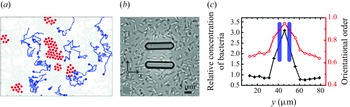


 Open access