




1 Introduction
Gravity currents are flows driven by horizontal density variations. There are many examples of gravity currents, both naturally occurring and man-made (Simpson Reference Simpson1997). Gravity currents can propagate along a smooth boundary in an ambient fluid that is either homogeneous (e.g. Shin, Dalziel & Linden Reference Shin, Dalziel and Linden2004; Cantero et al. Reference Cantero, Lee, Balachandar and Garcia2007; Ooi, Constantinescu & Weber Reference Ooi, Constantinescu and Weber2009) or stably stratified (e.g. Birman & Meiburg Reference Birman and Meiburg2007; Venayagamoorthy & Fringer Reference Venayagamoorthy and Fringer2007; Nicholson & Flynn Reference Nicholson and Flynn2015; Nasr-Azadani & Meiburg Reference Nasr-Azadani and Meiburg2016). During the advancement of a gravity current, it may be subject to the influences of bottom roughness/submerged canopies consisting of distributed drag elements that occupy a portion of the flow depth. A handful of previous studies have dealt with gravity currents interacting with a submerged canopy in a homogeneous ambient. For example, Cenedese, Nokes & Hyatt (Reference Cenedese, Nokes and Hyatt2018) experimentally investigated the dilution of gravity currents over an array of cylinders. They proposed that for a sparse canopy, the current propagates through the canopy interior (i.e. through-flow), with the individual cylinder wakes being the main contributor to the current dilution; in contrast, for a dense canopy, the current rides on top of it (i.e. over-flow) and the dilution is mainly driven by the vertical convection between the dense current and the underlying lighter fluid within the pore regions. Using experiments and large-eddy simulations (LES), Zhou et al. (Reference Zhou, Cenedese, Williams, Ball, Venayagamoorthy and Nokes2017) found a non-monotonic relationship between gravity current front velocity and canopy density (i.e. solid volume fraction), which has been attributed to the transition from through-flow to over-flow as the canopy density increases.
Gravity currents propagating in an ambient fluid with vertical density stratification are common in lakes, estuaries, coastal oceans and the atmosphere. However, to the best of our knowledge, all existing studies in the literature have only focused on the current–canopy interactions in a homogeneous ambient (e.g. Zhang & Nepf Reference Zhang and Nepf2011; Ozan, Constantinescu & Nepf Reference Ozan, Constantinescu and Nepf2016; Ottolenghi, Cenedese & Adduce Reference Ottolenghi, Cenedese and Adduce2017; Zhou et al. Reference Zhou, Cenedese, Williams, Ball, Venayagamoorthy and Nokes2017; Cenedese et al. Reference Cenedese, Nokes and Hyatt2018). Therefore, a clear understanding of the impact of ambient stable stratification on such flows is lacking. In this study, we investigate for the first time the dynamics of bottom gravity currents propagating over a long canopy submerged in a linearly stratified ambient using highly resolved three-dimensional LES.
Figure 1 shows the full-depth lock-release configuration used in this study. The channel has a height of  $H$ (i.e. the total flow depth) and a width of $W$. The canopy is composed of $n$ square cylinders with a staggered arrangement. The size of the individual square cylinders is $d$ in edge length (fixed throughout) and $h$ in height. The longitudinal and lateral centre-to-centre cylinder spacings are set to be equal, i.e. $s_{x}=s_{y}$. The offset rows are shifted by $s_{y}/2$ along the lateral direction. Canopy geometry in the horizontal plane is characterized by the canopy density (i.e. the solid volume fraction):
 $$\begin{eqnarray}\unicode[STIX]{x1D719}={\displaystyle \frac{V_{solids}}{V_{canopy}}}={\displaystyle \frac{nd^{2}h}{WhL_{canopy}}},\end{eqnarray}$$
 where  $L_{canopy}$ is the streamwise extent of the canopy region. Two values of canopy height (short canopies with $h=2.5d$ and tall canopies with $h=5d$) will be considered to investigate the effect of non-dimensional canopy height $h/H$. Note that a more appropriate non-dimensional geometrical parameter would be $ah$ where $a=d/(s_{x}s_{y})=nd/(WL_{canopy})$ is the frontal area per canopy volume (e.g. Rominger & Nepf Reference Rominger and Nepf2011; Nepf Reference Nepf2012). However, due to the geometrically similar canopies considered in this study, $\unicode[STIX]{x1D719}$ is linearly proportional to $ah$ for a certain canopy height and thus serves as a proper representation of canopy geometry. With the configurations considered in this study, given that $ah=\unicode[STIX]{x1D719}(h/d)$, we have $ah=2.5\unicode[STIX]{x1D719}$ for the short canopies and $5\unicode[STIX]{x1D719}$ for the tall canopies.
Before gate removal, the current density is  $\unicode[STIX]{x1D70C}_{c}$, and the ambient linear stratification is prescribed as $\unicode[STIX]{x1D70C}(z)=\unicode[STIX]{x1D70C}_{b}-(\unicode[STIX]{x1D70C}_{b}-\unicode[STIX]{x1D70C}_{0})z/H$, with $z$ starting at the bed and pointing upwards. Here, $\unicode[STIX]{x1D70C}_{0}$ and $\unicode[STIX]{x1D70C}_{b}$ are the surface and bottom densities of the ambient fluid, respectively. Based on physical scaling and experiments, Maxworthy et al. (Reference Maxworthy, Leilich, Simpson and Meiburg2002) proposed a functional relationship between the gravity current Froude number and a dimensionless parameter $R$ which measures the strength of the current ( $\unicode[STIX]{x1D70C}_{c}-\unicode[STIX]{x1D70C}_{0}$) relative to the strength of the ambient stratification ( $\unicode[STIX]{x1D70C}_{b}-\unicode[STIX]{x1D70C}_{0}$):
 $$\begin{eqnarray}R={\displaystyle \frac{\unicode[STIX]{x1D70C}_{c}-\unicode[STIX]{x1D70C}_{0}}{\unicode[STIX]{x1D70C}_{b}-\unicode[STIX]{x1D70C}_{0}}}={\displaystyle \frac{N_{c}^{2}}{N^{2}}},\end{eqnarray}$$
 where  $N=\sqrt{g(\unicode[STIX]{x1D70C}_{b}-\unicode[STIX]{x1D70C}_{0})/\unicode[STIX]{x1D70C}_{0}H}$ is the buoyancy frequency of the ambient stratification, and $N_{c}=\sqrt{g(\unicode[STIX]{x1D70C}_{c}-\unicode[STIX]{x1D70C}_{0})/\unicode[STIX]{x1D70C}_{0}H}$ is a fictitious buoyancy frequency calculated using the initial current density. It is worth noting that $N_{c}$ (by definition) is a measure of the overturning timescale ( $H/U$) of the gravity current with $U$ being the front velocity. In the present study, the dynamics of current–canopy interaction in the $\unicode[STIX]{x1D719}$– $R$ parameter space will be systematically investigated. The variation of $R$ will be realized by varying $\unicode[STIX]{x1D70C}_{b}$ while both $\unicode[STIX]{x1D70C}_{c}$ and $\unicode[STIX]{x1D70C}_{0}$ are kept constant (i.e. $N_{c}$ is constant). Therefore, $1/R\propto N^{2}$ serves as an indicator of the strength of the ambient stratification.
At a fundamental level, this study will introduce canopy drag to the scenarios in Maxworthy et al. (Reference Maxworthy, Leilich, Simpson and Meiburg2002) (smooth bed in a stratified ambient), and introduce ambient stratification to the scenarios in Zhou et al. (Reference Zhou, Cenedese, Williams, Ball, Venayagamoorthy and Nokes2017) (submerged canopy in a homogeneous ambient). The research questions that will be answered are: (i) How does the ambient stratification affect the pathway of current propagation (either through or above the canopy)? (ii) How does the ambient stratification modulate the entrainment and dilution of the current? and (iii) What are the implications of (i) and (ii) for the current front velocity?
Schematic diagram showing the computational domain and set-up (not to scale): (a) side view; (b) plan view. The dashed line indicates the lock gate at  $x=0$. A passive tracer is added to the lock fluid ( $-L_{lock}\leqslant x<0$) with an initial concentration of $c_{0}=1$ ( $c_{0}=0$ in the ambient fluid).

Canopies from different systems with different scales exhibit a wide range of  $\unicode[STIX]{x1D719}$. For aquatic canopies, $\unicode[STIX]{x1D719}$ ranges from 0.001 for marsh grasses to 0.45 for mangroves (Nepf Reference Nepf2012). In atmospheric settings, there is an even wider range of $\unicode[STIX]{x1D719}$ ( $\unicode[STIX]{x1D719}\approx 0$ in the open country and $\unicode[STIX]{x1D719}\approx 1$ in a dense urban centre). In this regard, we will investigate the current–canopy interactions over the full range of $\unicode[STIX]{x1D719}$ (i.e. from 0 to 1). In addition, the ambient fluid will be varied as homogeneous, weakly stratified and strongly stratified to explore its dynamical effects. Although the present study may not immediately (and directly) represent the forcing and geometry associated with the various real systems, the insights gained have broad practical relevance, e.g. buoyant river plumes interacting with kelp forests in the stratified coastal ocean, salt wedges propagating over bottom roughness in estuaries with tidal variations in stratification, and atmospheric gravity fronts (e.g. haboobs and sea breezes) advancing through urban canopies under stable stratification.
In what follows, § 2 describes the numerical model employed and the set-up of the LES runs. Sections 3–5 focus on the flow dynamics in the  $\unicode[STIX]{x1D719}$– $R$ parameter space with a constant non-dimensional canopy height of $h/H=1/4$. Section 3 provides an overview of the propagation regimes of the gravity current as a function of canopy density and ambient stratification. The dynamics of entrainment and dilution of the current is discussed in § 4. Based on these, § 5 is dedicated to the modulation of front velocity by the ambient stratification. The effect of $h/H$ is briefly discussed in § 6. Finally, conclusions are drawn in § 7.
2 Numerical model and set-up
The LES-filtered Navier–Stokes equations with the Boussinesq approximation are given in tensor notation by
 $$\begin{eqnarray}\frac{\unicode[STIX]{x2202}u_{i}}{\unicode[STIX]{x2202}t}+\frac{\unicode[STIX]{x2202}(u_{i}u_{j})}{\unicode[STIX]{x2202}x_{j}}=-\frac{1}{\unicode[STIX]{x1D70C}_{0}}\frac{\unicode[STIX]{x2202}p}{\unicode[STIX]{x2202}x_{i}}+\unicode[STIX]{x1D708}\frac{\unicode[STIX]{x2202}^{2}u_{i}}{\unicode[STIX]{x2202}x_{j}\unicode[STIX]{x2202}x_{j}}-g\frac{\unicode[STIX]{x1D70C}}{\unicode[STIX]{x1D70C}_{0}}\unicode[STIX]{x1D6FF}_{i3}-\frac{\unicode[STIX]{x2202}\unicode[STIX]{x1D70F}_{ij}^{SGS}}{\unicode[STIX]{x2202}x_{j}},\end{eqnarray}$$
subject to the filtered continuity equation
 $$\begin{eqnarray}\frac{\unicode[STIX]{x2202}u_{i}}{\unicode[STIX]{x2202}x_{i}}=0,\end{eqnarray}$$
and the filtered density transport equation
 $$\begin{eqnarray}\frac{\unicode[STIX]{x2202}\unicode[STIX]{x1D70C}}{\unicode[STIX]{x2202}t}+\frac{\unicode[STIX]{x2202}(\unicode[STIX]{x1D70C}u_{j})}{\unicode[STIX]{x2202}x_{j}}=\unicode[STIX]{x1D705}\frac{\unicode[STIX]{x2202}^{2}\unicode[STIX]{x1D70C}}{\unicode[STIX]{x2202}x_{j}\unicode[STIX]{x2202}x_{j}}-\frac{\unicode[STIX]{x2202}\unicode[STIX]{x1D712}_{j}^{SGS}}{\unicode[STIX]{x2202}x_{j}},\end{eqnarray}$$
 where  $\unicode[STIX]{x1D708}$ is the (constant) kinematic viscosity, $\unicode[STIX]{x1D705}$ is the (constant) scalar diffusivity, $\unicode[STIX]{x1D70F}_{ij}^{SGS}$ is the subgrid-scale (SGS) stress tensor and $\unicode[STIX]{x1D712}_{j}^{SGS}$ is the SGS scalar flux vector. The indices $i=1,2,3$ indicate the $x$ (longitudinal), $y$ (lateral) and $z$ (vertical) directions, respectively. Equations (2.1)–(2.3) are computed using the computational fluid dynamics software, FLOW-3D. The Fractional Area–Volume Obstacle Representation technique ( $FAVOR^{TM}$, Hirt Reference Hirt1993) enables the model to change the embedded geometry realistically without changing the mesh, which is considered superior for the present study. The second-order, monotonicity-preserving upwind-differencing method (van Leer Reference van Leer1977) is applied to approximate the momentum and density advection.
This numerical model has been extensively validated for various buoyancy-driven flow and canopy flow problems, e.g. particle-driven gravity currents (An, Julien & Venayagamoorthy Reference An, Julien and Venayagamoorthy2012), intrusive gravity currents encountering an obstacle in a linearly stratified ambient (Zhou & Venayagamoorthy Reference Zhou and Venayagamoorthy2017) and the hydrodynamics of a suspended canopy patch (Zhou & Venayagamoorthy Reference Zhou and Venayagamoorthy2019). The particularly relevant work of Zhou et al. (Reference Zhou, Cenedese, Williams, Ball, Venayagamoorthy and Nokes2017) investigated the propagation of gravity currents over a submerged canopy in a homogeneous ambient, where LES using the same code successfully reproduced the experimentally measured front speed and mixing pattern of the gravity current as it interacts with the canopy. In the context of gravity currents in stratified environments, additional simulations were conducted to further validate the code. A Cartesian mesh with a resolution of  $0.125d$ was used (see figure 1 for the definition of $d$). Figure 2 shows the positional history of the gravity current front propagating along a smooth bed in a linearly stratified fluid, where the agreement between the present LES and the experimental data from Maxworthy et al. (Reference Maxworthy, Leilich, Simpson and Meiburg2002) is excellent.
Model validation: positional history of the gravity current front on a smooth bed (i.e.  $\unicode[STIX]{x1D719}=0$) in a linearly stratified fluid. Results from the present LES (solid lines) are compared with experimental data (markers, from Maxworthy et al. Reference Maxworthy, Leilich, Simpson and Meiburg2002).

The numerical set-up used in this study is shown in figure 1. LES were conducted in a computational domain with dimensions of  $45H\times 1.2H\times H$ (i.e. length $\times$ width $\times$ depth). The longitudinal extents of the lock region, canopy region, and buffer region are $L_{lock}=5H$, $L_{canopy}=15H$, and $L_{buffer}=25H$, respectively. The domain top boundary was modelled as a free-slip rigid lid, while all the solid surfaces were treated as no-slip walls. The same mesh resolution that was used for the model validation ( $0.125d$) was applied throughout the whole computational domain of all the simulation runs. Only bottom-propagating gravity current ( $\unicode[STIX]{x1D70C}_{c}>\unicode[STIX]{x1D70C}_{b}$, i.e. $R>1$) is considered such that the case of intrusive gravity currents ( $\unicode[STIX]{x1D70C}_{0}<\unicode[STIX]{x1D70C}_{c}<\unicode[STIX]{x1D70C}_{b}$) is excluded.
Two values of non-dimensional canopy height are considered,  $h/H=1/4$ and $1/2$, which fall into the category of shallow submergence (Nepf Reference Nepf2012). These particular values of submergence ratio were chosen for the following reasons: (i) because of the limitation of light penetration, most submerged aquatic canopies occur in the range of shallow submergence (Duarte Reference Duarte1991); (ii) gravity currents propagating through and over a shallowly submerged canopy are in a transitional state between the through-flow and over-flow regimes, thus exhibiting the richest set of flow behaviours in the $\unicode[STIX]{x1D719}$– $R$ parameter space. For very deep submergence, the current would be largely within the over-flow regime and subject to negligible effect from the canopy drag; for emergent canopies, the current has to find its way through the canopy interior without any overtopping. Except for these two extremities, it is conceivable that the qualitative aspects of the results presented in this paper can also be applied to scenarios with other intermediate submergence ratios. In §§ 3–5, simulations are performed with a fixed value of $h/H=1/4$ in order to focus on the variation of flow dynamics in the $\unicode[STIX]{x1D719}$– $R$ parameter space. In § 6, a relatively taller canopy ( $h/H=1/2$) is considered to investigate the effect of varying $h/H$.
The invariant and varied model parameters are summarized in table 1. The variation of canopy density  $\unicode[STIX]{x1D719}$ is realized by varying the number of cylinders $n$ in the canopy region while keeping $s_{x}=s_{y}$ (i.e. staggered arrangement); the variation of current-to-stratification strength parameter $R$ is realized by varying the ambient bottom density $\unicode[STIX]{x1D70C}_{b}$ while keeping $\unicode[STIX]{x1D70C}_{c}$ and $\unicode[STIX]{x1D70C}_{0}$ constant; and the variation of non-dimensional canopy height $h/H$ is realized by varying the canopy height $h$ while keeping $H$ constant. This results in a velocity scale that is constant across all the LES runs:
 $$\begin{eqnarray}N_{c}H=\sqrt{g^{\prime }H},\end{eqnarray}$$
 where  $N_{c}=1.213~\text{s}^{-1}$ and $g^{\prime }=g(\unicode[STIX]{x1D70C}_{c}-\unicode[STIX]{x1D70C}_{0})/\unicode[STIX]{x1D70C}_{0}=0.294~\text{m}~\text{s}^{-2}$. In § 5, $N_{c}H$ is used to scale the gravity current front velocity $U$ in order to compute the Froude number, i.e. $Fr=U/(N_{c}H)$. For all the runs, the channel Reynolds number is $Re_{H}=(N_{c}H)H/\unicode[STIX]{x1D708}\approx 50\,000$, and the cylinder Reynolds number is $Re_{d}=Ud/\unicode[STIX]{x1D708}\approx 1200{-}2200$.
Model parameters in this study. Invariant parameters include:  $\unicode[STIX]{x1D70C}_{c}=1030~\text{kg}~\text{m}^{-3}$, $\unicode[STIX]{x1D70C}_{0}=1000~\text{kg}~\text{m}^{-3}$ and $N_{c}=1.213~\text{s}^{-1}$. In §§ 3–5 (short canopies with $h/H=1/4$), $\unicode[STIX]{x1D719}$ was varied as 0.000, 0.074, 0.206, 0.297, 0.404, 0.529, 0.669, 0.826 and 1.000 (nine values of $\unicode[STIX]{x1D719}$) for each of the three values of $R$. In § 6 (tall canopies with $h/H=1/2$), $\unicode[STIX]{x1D719}$ was varied as 0.074 and 0.404 (two values of $\unicode[STIX]{x1D719}$), which are representative of sparse and dense canopies, respectively. There are a total of 33 LES runs, with a mesh count of 19.6 million for each run.

Time is rendered dimensionless by  $\tilde{t}=tN_{c}$. The fluid density is non-dimensionalized as
 $$\begin{eqnarray}\tilde{\unicode[STIX]{x1D70C}}={\displaystyle \frac{\unicode[STIX]{x1D70C}-\unicode[STIX]{x1D70C}_{0}}{\unicode[STIX]{x1D70C}_{c}-\unicode[STIX]{x1D70C}_{0}}}\in [0,1].\end{eqnarray}$$
 In order to track the location of the current, a passive tracer is added to the lock fluid with an initial (uniform) concentration of  $c_{0}=1$ ( $c_{0}=0$ in the ambient fluid). Therefore, similar to $\tilde{\unicode[STIX]{x1D70C}}$, we have $c\in [0,1]$ throughout the computational domain at any given time.
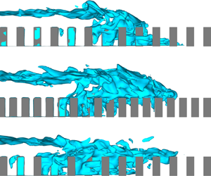
Instantaneous isosurface of tracer concentration at  $c=0.5$ for three reference scenarios with $h/H=1/4$ (side view at $\tilde{t}=30$). Cylinders are coloured in grey. Comparison of (a,b) shows the effect of increasing canopy density, while comparison of (a,c) shows the effect of strengthening ambient stratification.

Laterally averaged non-dimensional fluid density field superimposed by three contour lines of tracer concentration (white line:  $c=0.1$; grey line: $c=0.5$; black line: $c=0.9$). (a–c) $\unicode[STIX]{x1D719}=0.000$; (d–f) $\unicode[STIX]{x1D719}=0.074$; (g–i) $\unicode[STIX]{x1D719}=0.206$; (j–l) $\unicode[STIX]{x1D719}=0.404$. For all panels, the gravity current has propagated for a distance of $x_{f}=8H$. The non-dimensional canopy height is $h/H=1/4$.

3 Propagation regimes
As an overview, we show the instantaneous flow structure in figure 3 using the isosurface of tracer concentration at  $c=0.5$ for three reference scenarios with $h/H=1/4$ (i.e. short canopies). It can be seen that the propagation pathway of the gravity current is a function of both canopy density and ambient stratification. The effect of $\unicode[STIX]{x1D719}$ on the current propagation in a homogeneous ambient ( $R=\infty$) as found by Zhou et al. (Reference Zhou, Cenedese, Williams, Ball, Venayagamoorthy and Nokes2017) and Cenedese et al. (Reference Cenedese, Nokes and Hyatt2018) is qualitatively reproduced by comparing figures 3(a) and 3(b): the current nose initially propagates through the canopy interior when $\unicode[STIX]{x1D719}$ is small (figure 3a, referred to as the through-nose or TN for brevity); an increase of the canopy density leads to the formation of a secondary well-defined current nose that propagates over the canopy top (figure 3b, referred to as the over-nose or ON for brevity). On the other hand, the comparison of figures 3(a) and 3(c) showcases one of the key findings of this study: the intensification of ambient stratification (the decrease of $R$) has a similar effect to that of increasing $\unicode[STIX]{x1D719}$ on the diversion of current nose from along the bed to over the canopy top. In the rest of this paper, this process will be referred to as the through-to-over flow transition, which can be caused by both densification of canopy and intensification of ambient stratification.
Laterally averaged contours of non-dimensional fluid density  $\tilde{\unicode[STIX]{x1D70C}}$ and tracer concentration c in figure 4 show more quantitatively the effects of $\unicode[STIX]{x1D719}$ and $R$ on the propagation regimes. With $R$ kept constant, the increase of $\unicode[STIX]{x1D719}$ promotes the through-to-over flow transition. For example, as $\unicode[STIX]{x1D719}$ is increased in the strongly stratified ambient ( $R=1.2$), the control of the overall longitudinal current propagation gradually transitions from being the through-nose (figure 4f) to the over-nose (figure 4i). As the canopy is densified further (figure 4l), the through-nose is further left behind and almost indiscernible. The contour of $c=0.1$ (white line) in the canopy region beneath the over-current in figure 4(l) signifies the expanded area of vertical convection due to the unstable stratification between the over-current (larger $\tilde{\unicode[STIX]{x1D70C}}$ and $c>0$) and the underlying ambient fluid (smaller $\tilde{\unicode[STIX]{x1D70C}}$ and $c=0$). These observations confirm that the through-to-over flow transition caused by canopy densification in homogeneous environments also takes place in stratified environments. It is interesting to note that the presence of the submerged canopy dramatically inhibits the Kelvin–Helmholtz billows at the top interface of the current in the tail region (compare the flat-bed cases with the canopy-obstructed cases in figure 4). Similar phenomenon has been observed in two-layer flow down a rough slope where the formation and collapsing mechanism of Kelvin–Helmholtz instabilities are inhibited (Negretti, Zhu & Jirka Reference Negretti, Zhu and Jirka2008).
More details of the effect of ambient stratification on the current propagation regimes as shown in figure 3 are provided in figure 4. In figure 4(a–c), the Kelvin–Helmholtz billows at the top interface of the current tend to be suppressed by stronger ambient stratification (Turner Reference Turner1973). Besides this, the smaller gravity current front speed with smaller values of  $R$ (see § 5) leads to less vertical variation of horizontal shear between the current and the overlying return flow, which further stabilizes the stratified shear layer at the top interface. Given a sufficiently dense canopy, strengthening ambient stratification promotes the through-to-over flow transition (e.g. see the contours of $c=0.1$ in figure 4g–i), albeit through a different mechanism with respect to the variation of $\unicode[STIX]{x1D719}$. Instead of increasing the canopy drag, a decrease of $R$ weakens the effective buoyancy forcing that drives the current propagation within the canopy: stronger ambient stratification results in heavier ambient fluid, reducing the longitudinal internal pressure gradient between the current and the ambient fluid directly downstream. Consequently, the current tends to propagate at a higher level in the water column due to the smaller ambient density thereat (and thus stronger effective buoyancy forcing). Together with the retarding effect of the canopy drag, the decrease of $R$ leads to a gradual diversion of the current nose towards the canopy’s top boundary. For a very dense canopy (figure 4j–l), the current is within the over-flow regime even in the homogeneous ambient, and the intensification of ambient stratification leads to a growing dominance of the over-nose on the through-nose. This is reflected by the expanding low-concentration region (e.g. $c=0.1$) beneath the over-nose as $R$ decreases in figure 4(j–l), i.e. the through-nose is increasingly left behind until almost indiscernible. For a very sparse canopy (figure 4d–f), the through-to-over flow transition driven by the stronger ambient stratification is inconspicuous due to the insufficient canopy drag.
4 Entrainment and dilution
4.1 Quantification method
The mixing of the gravity current with the ambient fluid is important for geophysical applications, e.g. front propagation speed and sediment entrainment/deposition. In this study, during the advancement of the current front, the reduction of tracer concentration in the gravity current measures the entrainment of ambient fluid into the current, while the reduction of current fluid density reflects the dilution that effectively weakens the buoyancy forcing of the current propagation. In what follows, we investigate the dynamics of entrainment and dilution for gravity currents as a function of canopy density and ambient stratification for the short canopies ( $h/H=1/4$). After the gate removal, the entrainment is quantified by computing the change of spatially averaged tracer concentration relative to its initial value ( $\overline{c}_{0}=1$),
 $$\begin{eqnarray}E=1-\overline{c}={\displaystyle \frac{\displaystyle \int _{\unicode[STIX]{x1D6FA}}\unicode[STIX]{x1D6FC}\cdot (1-c)\,\text{d}V}{\displaystyle \int _{\unicode[STIX]{x1D6FA}}\unicode[STIX]{x1D6FC}\,\text{d}V}},\end{eqnarray}$$
 and the dilution is quantified by computing the change of spatially averaged non-dimensional fluid density relative to its initial value ( $\overline{\tilde{\unicode[STIX]{x1D70C}}}_{0}=1$),
 $$\begin{eqnarray}D=1-\overline{\tilde{\unicode[STIX]{x1D70C}}}={\displaystyle \frac{\displaystyle \int _{\unicode[STIX]{x1D6FA}}\unicode[STIX]{x1D6FC}\cdot (1-\tilde{\unicode[STIX]{x1D70C}})\,\text{d}V}{\displaystyle \int _{\unicode[STIX]{x1D6FA}}\unicode[STIX]{x1D6FC}\,\text{d}V}},\end{eqnarray}$$
 where the overbar indicates spatial averaging, and  $\unicode[STIX]{x1D6FC}$ is an identifier of the gravity current body (i.e. the contaminated lock fluid):
 $$\begin{eqnarray}\unicode[STIX]{x1D6FC}=\left\{\begin{array}{@{}ll@{}}1,\quad & 0.01\leqslant c\leqslant 1,\\ 0,\quad & 0\leqslant c<0.01.\end{array}\right.\end{eqnarray}$$
 Several previous studies on gravity currents propagating in a homogeneous ambient have quantified the mixing by computing the variation of the subvolume of the flow domain where the tracer concentration exceeds a given threshold value that is larger than that of the ambient fluid (Necker et al. Reference Necker, Hartel, Kleiser and Meiburg2005; Tokyay, Constantinescu & Merburg Reference Tokyay, Constantinescu and Merburg2011, Reference Tokyay, Constantinescu and Merburg2014), i.e.  $\int _{\unicode[STIX]{x1D6FA}}\unicode[STIX]{x1D6FC}\,\text{d}V$ (the denominator in (4.1) and (4.2)). Taking a step further, equations (4.1) and (4.2) enable us to distinguish between the entrainment (quantified by $E$) and dilution (quantified by $D$) so as to investigate their interrelationship as a function of time (or front location).
We consider two different control volumes  $\unicode[STIX]{x1D6FA}$ for the computations of (4.1)–(4.2). For localized mixing near the current front, $\unicode[STIX]{x1D6FA}=\unicode[STIX]{x1D6FA}_{f}$ is a moving fixed-size control volume which starts at the leading edge of the current front and extends $2H$ towards the tail region (in the frame of reference of the propagating current front):
 $$\begin{eqnarray}E_{f}={\displaystyle \frac{\displaystyle \int _{x_{f}-2H}^{x_{f}}\displaystyle \int _{0}^{H}\displaystyle \int _{0}^{W}\unicode[STIX]{x1D6FC}\cdot (1-c)\,\text{d}V}{\displaystyle \int _{\unicode[STIX]{x1D6FA}}\unicode[STIX]{x1D6FC}\,\text{d}V}},\quad D_{f}={\displaystyle \frac{\displaystyle \int _{x_{f}-2H}^{x_{f}}\displaystyle \int _{0}^{H}\displaystyle \int _{0}^{W}\unicode[STIX]{x1D6FC}\cdot (1-\tilde{\unicode[STIX]{x1D70C}})\,\text{d}V}{\displaystyle \int _{\unicode[STIX]{x1D6FA}}\unicode[STIX]{x1D6FC}\,\text{d}V}},\end{eqnarray}$$
 where  $E_{f}$ and $D_{f}$ will be referred to as the front entrainment and front dilution, respectively. Here, the front position of the gravity current is determined by tracking the contour of $c=0.01$. For global mixing throughout the current body (including the front and tail regions), $\unicode[STIX]{x1D6FA}=\unicode[STIX]{x1D6FA}_{g}$ is a control volume encompassing the region between the lock gate and the current front, i.e. with a size that grows with time:
 $$\begin{eqnarray}E_{g}={\displaystyle \frac{\displaystyle \int _{0}^{x_{f}}\displaystyle \int _{0}^{H}\displaystyle \int _{0}^{W}\unicode[STIX]{x1D6FC}\cdot (1-c)\,\text{d}V}{\displaystyle \int _{\unicode[STIX]{x1D6FA}}\unicode[STIX]{x1D6FC}\,\text{d}V}},\quad D_{g}={\displaystyle \frac{\displaystyle \int _{0}^{x_{f}}\displaystyle \int _{0}^{H}\displaystyle \int _{0}^{W}\unicode[STIX]{x1D6FC}\cdot (1-\tilde{\unicode[STIX]{x1D70C}})\,\text{d}V}{\displaystyle \int _{\unicode[STIX]{x1D6FA}}\unicode[STIX]{x1D6FC}\,\text{d}V}},\end{eqnarray}$$
 where  $E_{g}$ and $D_{g}$ will be referred to as the global entrainment and global dilution, respectively. With these formulations, it directly follows that $E_{f}=E_{g}$ (and $D_{f}=D_{g}$) at $x_{f}=2H$. As shown in figure 5, as the current starts its propagation, front and global mixing start to diverge as more tail regions are included in the integrals of $E_{g}$ and $D_{g}$.
Entrainment and dilution as a function of the front position for different  $\unicode[STIX]{x1D719}$– $R$ combinations with $h/H=1/4$. Top panel shows the entrainment of ambient fluid into the current (4.1), while bottom panel shows the dilution that effectively weakens the longitudinal buoyancy forcing of the current (4.2). For both panels, solid lines represent the front mixing (4.4), while dotted lines represent the global mixing (4.5). (a,d) $\unicode[STIX]{x1D719}=0.000$; (b,e) $\unicode[STIX]{x1D719}=0.074$; (c,f) $\unicode[STIX]{x1D719}=0.404$.

4.2 Entrainment of ambient fluid
For the flat-bed cases (figure 5a), global entrainment  $E_{g}$ increases as the current propagates, while front entrainment $E_{f}$ almost stays the same. This clearly indicates that due to the absence of the canopy drag, entrainment is mainly driven by the interfacial Kelvin–Helmholtz billows which engulf ambient fluid in the tail region, which is consistent with figure 4(a–c).
The introduction of canopy drag significantly modifies the entrainment dynamics. In both figures 5(b) and 5(c), the front entrainment  $E_{f}$ is observed to remarkably increase with $x_{f}$. At $x_{f}=8H$, $E_{f}$ in these canopy-obstructed cases is much larger than in the flat-bed cases. In figure 5(b), the canopy is sparse such that the current is in the through-flow regime (see figure 4d–f), with the individual cylinder wakes acting as the main contributor to the entrainment of ambient fluid. In figure 5(c), the canopy is dense such that the current has transitioned to the over-flow regime (see figure 4j–l). In this case, consistent with Zhou et al. (Reference Zhou, Cenedese, Williams, Ball, Venayagamoorthy and Nokes2017) and Cenedese et al. (Reference Cenedese, Nokes and Hyatt2018), the entrainment is further enhanced by the vertical convection between the dense current and the underlying lighter fluid within the canopy. This is manifested by the increasing separation between the three contour lines of $c=0.1$, 0.5 and 0.9 in figure 4 as the gravity current transitions from through-flow to over-flow when the canopy is denser (e.g. compare figures 4e and 4k). We would like to stress that in figure 5 a small amount of roughness ( $\unicode[STIX]{x1D719}=0.074$) is able to trigger a significant enhancement of entrainment; a further increase to $\unicode[STIX]{x1D719}=0.404$ leads to a less prominent enhancement as the primary entraining mechanism switches from cylinder wakes to vertical convection (compare figures 5b and 5c).
Due to the suppression of Kelvin–Helmholtz billows in the tail region by the submerged canopy (see figure 4), the global entrainment  $E_{g}$ undergoes a relatively milder increase with respect to $E_{f}$. It should be noted that the lock region is long enough in this study to ensure sufficient supply of dense fluid to the canopy region. Although the global entrainment (and dilution) defined in (4.5) is increased by mixing occurring near the current front and in the tail region, it is also decreased by the dense fluid input from the left boundary of $\unicode[STIX]{x1D6FA}_{g}$ at $x_{f}=0$. At later stages of the canopy-obstructed cases (figure 5b,c), these counteracting effects almost reach an equilibrium so that $E_{g}$ shows a very weak dependence on $x_{f}$.
It is clear in figure 5(a–c) that for a certain canopy geometry, ambient stratification alone can affect the entrainment dynamics of the gravity current. In the flat-bed cases (figure 5a), less ambient fluid is entrained into the current (i.e. smaller  $E_{g}$) under stronger ambient stratification (smaller $R$) due to the suppression of Kelvin–Helmholtz instabilities at the current–ambient interface (visualized in figure 4a–c). On the other hand, for the canopy-obstructed cases (figure 5b,c), the front entrainment $E_{f}$ is enhanced by stronger ambient stratification. Manifested in figures 4(d–f) and 4(j–l) are the increasing separation between the three $c$-contours as $R$ decreases. The underlying physics governing this effect of $R$ on $E_{f}$ depend on the propagation regimes of the gravity current. For the sparse canopy (figure 5b), a decrease of $R$ leads to a smaller density difference between the current propagating along the bed and the surrounding ambient fluid (see figure 4d–f). As a result, although the ambient is internally more stratified, the weaker stratification between the dense current and the ambient allows the turbulent cylinder wakes to cause more intense exchange across the current–ambient interface, i.e. enhanced front entrainment in the through-flow regime. Differently, for the dense canopy (figure 5c), two mechanisms affect the entrainment but in opposite senses as $R$ decreases (see figure 4j–l): on one hand, the smaller density difference between the over-current propagating along the canopy top and the underlying ambient fluid weakens the convectively driven front entrainment; on the other hand, the over-nose shows a growing dominance on the through-nose as $R$ decreases, expanding the area of vertical convective instability in the canopy region beneath the over-current. Taken together, the second mechanism dominates, leading to stronger front entrainment at smaller $R$ in the over-flow regime. Moreover, the global entrainment $E_{g}$ of canopy-obstructed gravity currents shows a weak dependence on $R$, mainly due to the opposite dependencies of front mixing and tail mixing on ambient stratification.
4.3 Dilution of current density
By comparing figures 5(d), 5(e) and 5(f), it is seen that the variation of canopy density affects the dilution of current density in a similar manner to the entrainment. For a certain value of  $R$, an increase of $\unicode[STIX]{x1D719}$ enhances the entrainment of ambient fluid with the same internal density structure (i.e. vertical stratification). As expected, this results in enhanced dilution of the current density. This is consistent with the variation of density distributions as a function of $\unicode[STIX]{x1D719}$ in figure 4, e.g. compare figures 4(b), 4(e) and 4(k).
It can be seen in figure 5 that for homogeneous environments ( $R=\infty$), $E_{f}=D_{f}$ and $E_{g}=D_{g}$ because the fields of $c$ and $\tilde{\unicode[STIX]{x1D70C}}$ are identical. As ambient stratification strengthens, entrainment and dilution show increasingly notable differences between each other (i.e. $D_{f}/E_{f}$ becomes smaller). This can be observed for both the front mixing ( $E_{f}$ versus $D_{f}$) and the global mixing ( $E_{g}$ versus $D_{g}$). The explanation is that a decrease of $R$ results in a smaller density difference between the gravity current and the ambient fluid, thus causing less dilution of current density per unit volume of entrained fluid. This drop of current–ambient density difference with decreasing $R$ leads to weaker spatially averaged dilution despite the stronger front entrainment in canopy-obstructed cases. These observations are consistent with the variation of density distributions as a function of $R$ while keeping $\unicode[STIX]{x1D719}$ constant in figure 4 (e.g. see figure 4j–l).
To sum up, the introduction of ambient stratification brings more complexity to the mixing dynamics of gravity current through and over a submerged canopy in an otherwise homogeneous environment. Interfacial mixing in the tail region prevails in the flat-bed cases, while localized mixing near the current front is dominant in the canopy-obstructed cases. The key message from the above analysis is that the positive correlation between entrainment and dilution for current–canopy interactions in a homogeneous ambient does not necessarily hold for the case of a stratified ambient. Under a certain background stratification, the effect of canopy roughness is qualitatively similar between homogeneous and stratified ambients: both the entrainment and dilution are enhanced. For a given canopy density, stronger ambient stratification weakens the global entrainment in flat-bed cases, but enhances the front entrainment in canopy-obstructed cases. Nonetheless, the decrease of current-ambient density difference (a result of strengthening ambient stratification) tends to cause a weaker net dilution of the current density even though more ambient fluid is entrained.
5 Front velocity
5.1 Modulation of  $Fr$–$\unicode[STIX]{x1D719}$ relationship by ambient stratification


In this section, we explore how ambient stratification modulates the non-monotonic relationship between front velocity and canopy density as found by Zhou et al. (Reference Zhou, Cenedese, Williams, Ball, Venayagamoorthy and Nokes2017) in a homogeneous ambient. Only short canopies will be discussed here, with the effect of changing canopy height left to § 6. The positional history of the current front in three sample runs is shown in figure 6, where the frontmost nose of the contour of  $c=0.01$ was tracked (either through or over the canopy). The gravity current was found to propagate at a nearly constant speed in the slumping phase. Correspondingly, the Froude number (time averaged over the period of $\tilde{t}=6{-}30$) is determined by the frontmost nose:
 $$\begin{eqnarray}Fr=\text{max}\left\{{\displaystyle \frac{U_{TN}}{N_{c}H}},{\displaystyle \frac{U_{ON}}{N_{c}H}}\right\},\end{eqnarray}$$
 where  $U_{TN}$ and $U_{ON}$ are the front velocities of the through-nose and the over-nose, respectively. Note that the time-averaging operation is not written explicitly here. In addition, the Froude number is also normalized by $Fr_{\unicode[STIX]{x1D719}=0}$ which is the base value of the smooth-bed case (i.e. $\unicode[STIX]{x1D716}=Fr/Fr_{\unicode[STIX]{x1D719}=0}$) under the same ambient stratification. This provides a measure of the sensitivity of current propagation to the presence of the submerged canopy with the effect of different strengths of ambient stratification ruled out.
The parametric dependencies of  $Fr$ and $\unicode[STIX]{x1D716}$ for the short canopies ( $h/H=1/4$) are shown in figures 7(a) and 7(b), respectively. Note that the data for $h/H=1/2$ are also shown, but we defer the discussion of these tall canopies to § 6. For the smooth bed ( $\unicode[STIX]{x1D719}=0$), $Fr_{\unicode[STIX]{x1D719}=0}$ decreases with decreasing $R$ due to the weaker current strength compared with the stratification strength. As the canopy drag is introduced, $Fr$ begins to drop. For small values of $\unicode[STIX]{x1D719}$, the current propagates along the channel bed, and the reduction of $Fr$ with increasing $\unicode[STIX]{x1D719}$ is less prominent for smaller $R$ (i.e. $\unicode[STIX]{x1D716}$ is larger). This is mainly caused by the weakened density dilution under stronger ambient stratification as discussed in § 4. As $\unicode[STIX]{x1D719}$ increases further, $Fr$ gradually recovers in both homogeneous and stratified ambient environments. The most striking feature of figure 7 is that stronger ambient stratification causes the minimum $Fr$ to occur at a smaller value of $\unicode[STIX]{x1D719}$, i.e. $\unicode[STIX]{x1D719}=0.404$ for $R=\infty$, $\unicode[STIX]{x1D719}=0.297$ for $R=2$ and $\unicode[STIX]{x1D719}=0.206$ for $R=1.2$. This shift of the turning point towards smaller $\unicode[STIX]{x1D719}$ is mainly caused by the stronger ambient stratification that promotes the diversion of gravity current towards the canopy top (see figure 3). As found by Zhou et al. (Reference Zhou, Cenedese, Williams, Ball, Venayagamoorthy and Nokes2017), this through-to-over flow transition is a major mechanism for the recovery of $Fr$ as $\unicode[STIX]{x1D719}$ increases since the over-current is subject to less canopy drag.
Positional history of the gravity current front for three sample runs: a flat-bed case ( $\unicode[STIX]{x1D719}=0.000$, $R=\infty$), a through-flow case ( $\unicode[STIX]{x1D719}=0.074$, $R=2$) and an over-flow case ( $\unicode[STIX]{x1D719}=0.404$, $R=1.2$). Solid black lines are the linear fittings of the front positions during $\tilde{t}=6{-}30$. The non-dimensional canopy height is $h/H=1/4$.

Variation of gravity current front velocity in the  $\unicode[STIX]{x1D719}$– $R$ parameter space with $h/H=1/4$ (short canopies, marked by solid circles): (a) time-averaged Froude number in the slumping phase as defined by (5.1); (b) normalized Froude number. The vertical black, blue and red dashed lines indicate $\unicode[STIX]{x1D719}$-values with the smallest $Fr$ (and $\unicode[STIX]{x1D716}$) for runs with $R=\infty$, 2 and 1.2, respectively. The horizontal grey dotted lines mark the level of $Fr_{\unicode[STIX]{x1D719}=0}$ and $\unicode[STIX]{x1D716}_{\unicode[STIX]{x1D719}=0}$ for $R=1.2$. Note that the data for $h/H=1/2$ (tall canopies, marked by empty circles) are also shown but the discussion is deferred to § 6.

Another important feature of figure 7 is that different values of  $R$ may result in almost equally fast current propagation in the range of $\unicode[STIX]{x1D719}=0.404{-}0.669$ in figure 7(a). This is not possible for gravity currents propagating over a flat bed where $Fr$ monotonically increases with $R$ (Maxworthy et al. Reference Maxworthy, Leilich, Simpson and Meiburg2002). When normalized by the smooth-bed value ( $Fr_{\unicode[STIX]{x1D719}=0}$), this is manifested in figure 7(b) as the big gaps between the $\unicode[STIX]{x1D716}$-curves corresponding to different values of $R$, signifying that the propagation of gravity currents under stronger ambient stratification is less sensitive to the retarding effect of the submerged canopy. The earlier transition (in $\unicode[STIX]{x1D719}$) to over-flow discussed above is certainly a driver, but two additional mechanisms further contribute to increasing $\unicode[STIX]{x1D716}$ when the ambient stratification is strengthened: (i) as the current is lifted up by a vertical distance that amounts to the canopy height, the effective longitudinal buoyancy is stronger due to the accompanied reduction of local ambient fluid density directly downstream of the over-nose (i.e. more buoyancy gain, see § 3); (ii) the dilution of the over-current is weakened due to the smaller density difference between the current and the entrained ambient fluid (i.e. less buoyancy loss, see § 4). This second mechanism is confirmed by the fact that as $\unicode[STIX]{x1D719}$ increases beyond 0.669, the gaps between the $\unicode[STIX]{x1D716}$-curves in figure 7(b) become smaller because the current dilution due to vertical convection gradually vanishes as the pore regions shrink.
5.2 Formulation of $Fr_{\unicode[STIX]{x1D719}=1}$ as a function of $R$ and $h/H$


It is interesting to note that at  $R=1.2$ in figure 7, the Froude number shows an almost negligible reduction when it encounters a submerged solid slab with a height of $h$ (i.e. $Fr_{\unicode[STIX]{x1D719}=1}\approx Fr_{\unicode[STIX]{x1D719}=0}$). The reason is presumably that the buoyancy loss due to the smaller effective water depth ( $H-h$) and the buoyancy gain due to the upward displacement of the current nose cancel each other out. In what follows, we formulate $Fr_{\unicode[STIX]{x1D719}=1}$ as a function of $R$ and $h/H$ by modifying the empirical $Fr$–
$Fr$– $R$ relationship proposed by Maxworthy et al. (Reference Maxworthy, Leilich, Simpson and Meiburg2002) and compare it with our LES results. Upon the removal of the lock gate, suppose that the gravity current encounters a bottom-mounted solid slab with a height of $h$ that is submerged in a stratified ambient fluid with a depth of $H$. As the current is lifted up by a vertical distance of $h$, the effective water depth decreases from $H$ to $H-h$. Since the front velocity scales with the square root of water depth (see (2.4)), the modified Froude number can be expressed as $Fr_{\unicode[STIX]{x1D719}=1}=Fr_{\unicode[STIX]{x1D719}=0}\cdot (1-h/H)^{1/2}$. The determination of $Fr_{\unicode[STIX]{x1D719}=0}$ needs to be treated differently between homogeneous and stratified ambients: (i) for a homogeneous ambient, the experiments of Shin et al. (Reference Shin, Dalziel and Linden2004) indicates that $Fr_{\unicode[STIX]{x1D719}=0}=0.45$; (ii) for a linearly stratified ambient, Maxworthy et al. (Reference Maxworthy, Leilich, Simpson and Meiburg2002) shows from experiments that $Fr_{\unicode[STIX]{x1D719}=0,m}=U/NH=0.266+0.912\text{log}(R)$ for full-depth lock release, where the subscript $m$ indicates the Froude number defined by Maxworthy et al. (Reference Maxworthy, Leilich, Simpson and Meiburg2002). Replacing $NH$ with $N_{c}H$ ( $=\sqrt{g^{\prime }H}=\sqrt{g(\unicode[STIX]{x1D70C}_{c}-\unicode[STIX]{x1D70C}_{0})H/\unicode[STIX]{x1D70C}_{0}}$) which is the velocity scale used in (5.1) gives $Fr_{\unicode[STIX]{x1D719}=0}=[0.266+0.912\text{log}(R)]\cdot R^{-1/2}$ where $R^{-1/2}=N/N_{c}$. In addition, due to the through-to-over flow transition, ambient fluid density directly downstream of the over-nose changes from $\unicode[STIX]{x1D70C}_{b}$ to $\unicode[STIX]{x1D70C}_{b}-(\unicode[STIX]{x1D70C}_{b}-\unicode[STIX]{x1D70C}_{0})h/H$. According to (1.2), $R$ changes to $R/(1-h/H)$. Taken together, we arrive at the following expressions for $Fr_{\unicode[STIX]{x1D719}=1}$ as a function of $R$ and $h/H$. For a homogeneous ambient (i.e. $R=\infty$),
 $$\begin{eqnarray}Fr_{\unicode[STIX]{x1D719}=1}(h/H)=0.45\cdot (1-h/H)^{1/2},\end{eqnarray}$$
 and for a linearly stratified ambient ( $R\geqslant 1$),
 $$\begin{eqnarray}Fr_{\unicode[STIX]{x1D719}=1}(R,h/H)=\left[0.266+0.912\text{log}\left({\displaystyle \frac{R}{1-h/H}}\right)\right]\cdot \left({\displaystyle \frac{R}{1-h/H}}\right)^{-1/2}\cdot (1-h/H)^{1/2}.\end{eqnarray}$$
 Equations (5.2) and (5.3) are plotted in figure 8. LES values of  $Fr_{\unicode[STIX]{x1D719}=1}$ at $h/H=0$ (i.e. the flat-bed case in figure 7) and $h/H=1/4$ (i.e. the solid-slab case in figure 7) are superimposed, showing good agreement with the formulations. On one hand, $Fr_{\unicode[STIX]{x1D719}=1}$ tends to decrease with increasing $h/H$ due to the reduced effective water depth and the corresponding weaker longitudinal buoyancy forcing. On the other hand, under stronger ambient stratification, $Fr_{\unicode[STIX]{x1D719}=1}$ tends to increase because the lifted current nose gains more buoyancy as $h/H$ increases. The outcome is the less prominent reduction of $Fr_{\unicode[STIX]{x1D719}=1}$ with increasing $h/H$ at smaller values of $R$ in figure 8. For the strongest stratification considered here ( $R=1.2$), $h/H=0$ and $1/4$ result in almost identical values of $Fr_{\unicode[STIX]{x1D719}=1}$.
6 Effect of canopy height
In preceding sections (§§ 3–5), the dynamics of gravity current propagation in the  $\unicode[STIX]{x1D719}$– $R$ parameter space is presented with a constant non-dimensional canopy height of $h/H=1/4$ (referred to as the short canopies). Here, we discuss the sensitivity of the above results to varying canopy height by investigating the case of $h/H=1/2$ (referred to as the tall canopies). Two canopy densities are considered: a sparse canopy ( $\unicode[STIX]{x1D719}=0.074$) and a dense canopy ( $\unicode[STIX]{x1D719}=0.404$).


Comparison between figures 4 and 9 reveals the important role of canopy height in regulating the regimes of gravity current propagation. For the sparse canopy with  $\unicode[STIX]{x1D719}=0.074$, given the relatively small canopy drag, strengthening of the ambient stratification alone is not able to promote any through-to-over flow transition for both the short and the tall canopies. Despite this, the increase of $h/H$ leads to a notable expansion of regions with active canopy-induced mixing of gravity current and ambient fluid, i.e. regions where cylinders protrude into the ambient fluid. Manifested in figure 9(a–c) are the more intersections of the three $c$-contours with the cylinders with respect to those in figure 4(d–f). This phenomenon has important implications for the mixing dynamics of gravity currents, as will be discussed below in figure 10. In contrast, for the dense canopy with $\unicode[STIX]{x1D719}=0.404$, the increase of $h/H$ from $1/4$ (figure 4j–l) to $1/2$ (figure 9d–f) results in remarkable changes of the propagation regimes. As the ambient stratification strengthens, while all of the three scenarios with short and dense canopies in figure 4(j–l) fall into the over-flow regime, gravity current encountering the tall and dense canopy transitions from through-flow (only through-nose, figure 9d) to intermediate-flow (through- and over-noses coexist, figure 9e), and finally over-flow (only over-nose, figure 9f). The difference between figures 4(j–l) and 9(d–f) can be explained by the fact that as a dense canopy becomes taller, the gravity current is more inclined to propagate along the bed instead of over the canopy’s top boundary because more potential energy is needed for the through-to-over flow transition to take place. Due to the excessive canopy drag that scales with $ah$ (Nepf Reference Nepf2012), impoundment of dense fluid can be observed in the upstream tail regions in figure 9(d–f).
Tall canopies ( $h/H=1/2$): laterally averaged non-dimensional fluid density field superimposed by three contour lines of tracer concentration. (a–c) $\unicode[STIX]{x1D719}=0.074$; (d–f) $\unicode[STIX]{x1D719}=0.404$. See caption of figure 4 for details.

Tall canopies ( $h/H=1/2$): entrainment and dilution as a function of the front position for different $\unicode[STIX]{x1D719}$– $R$ combinations. (a,c) $\unicode[STIX]{x1D719}=0.074$; (b,d) $\unicode[STIX]{x1D719}=0.404$. See caption of figure 5 for details. For comparison, the values of $E$ and $D$ at $x_{f}=8H$ for the short canopies ( $h/H=1/4$) in figure 5 are marked on the right: front mixing (circle symbols); global mixing (plus symbols).

Figure 10 demonstrates the effect of changing canopy height on the mixing dynamics. The evolutions of entrainment ( $E$) and dilution ( $D$) as a function of front location for the tall canopies are seen to be qualitatively similar to those for the short canopies in figure 5. This confirms that the conclusions drawn in § 4 regarding the effect of $\unicode[STIX]{x1D719}$ and $R$ on entrainment and dilution also apply to taller canopies: (i) the presence of the submerged canopy leads to locally enhanced entrainment and dilution near the current front; (ii) for a given canopy density, stronger ambient stratification enhances the front entrainment, but the front dilution is indeed weaker because of the smaller density difference between gravity current and ambient fluid. Despite these similarities, there are still several noticeable changes of the mixing dynamics due to the increase of canopy height when comparing canopies with different $h/H$ in figure 10. For the sparse canopy with $\unicode[STIX]{x1D719}=0.074$ (figure 10a,c), due to the expanded regions with active canopy-induced mixing as shown in figure 9(a–c), the overall magnitudes of entrainment and dilution are stronger for the taller canopy (i.e. $E_{h/H=1/2}>E_{h/H=1/4}$ and $D_{h/H=1/2}>D_{h/H=1/4}$ at $x_{f}=8H$). For the dense canopy with $\unicode[STIX]{x1D719}=0.404$, the flow-regime transition as $h/H$ increases also modifies the underlying mechanism for entrainment in figure 10(b,d) with respect to those in figure 5(c,f). On one hand, in the homogeneous ambient ( $R=\infty$), the current transitions from over-flow for the short canopy (figure 4j) to through-flow for the tall canopy (figure 9d). This is accompanied by a slightly weaker front entrainment $E_{f}$ at $x_{f}=8H$ with respect to the short canopy in figure 10(b). On the other hand, as the canopy is heightened in the stratified ambient environments ( $R=2$ and 1.2), the current is still partially or completely within the over-flow regime (figure 9e,f). Therefore, the over-nose is thinner and subject to stronger vertical convection inside the canopy compared with the case of a short canopy; there is a larger amount of ambient fluid beneath the over-nose, and the unstable stratification across the canopy’s top boundary is stronger since the dense current is propagating at a higher level in the water column. These flow-regime transitions due to increasing canopy height result in the interesting fact that when compared with the short and dense canopy, the front entrainment for the case of the tall and dense canopy is weaker at $R=\infty$ (i.e. $E_{f,h/H=1/2}<E_{f,h/H=1/4}$ at $x_{f}=8H$) but stronger at $R=2$ and 1.2 (i.e. $E_{f,h/H=1/2}>E_{f,h/H=1/4}$ at $x_{f}=8H$). This counteracts the smaller current–ambient density difference as $R$ decreases, resulting in smaller differences in front dilution between different strengths of ambient stratification for the taller canopy (note the smaller gaps between $D_{f}$-values at $x_{f}=8H$ for the tall-canopy cases with respect to the short-canopy cases in figure 10d). Moreover, regarding the global entrainment and dilution, it should be noted that the drop of $E_{g}$ and $D_{g}$ during certain phases of the current propagation in figure 10(b,d) is due to the expanding region of dense-fluid impoundment as the current advances downstream (figure 9d–f).
Increasing the canopy height also modulates the gravity current front velocity. When the slumping-phase Froude number of the six tall-canopy scenarios is normalized by the base value of the smooth-bed case under the same ambient stratification (i.e.  $\unicode[STIX]{x1D716}=Fr/Fr_{\unicode[STIX]{x1D719}=0}$), figure 7(b) confirms the applicability of one of the key findings in § 5 to taller canopies: the propagation of gravity currents under stronger ambient stratification is less sensitive to the retarding effect of the submerged canopy. For the tall and sparse canopy ( $h/H=1/2$, $\unicode[STIX]{x1D719}=0.074$), since no flow-regime transition occurs as ambient stratification is strengthened (figure 9a–c), the weaker current dilution (figure 10c) is the only mechanism that leads to the larger value of $\unicode[STIX]{x1D716}$ corresponding to smaller $R$ in figure 7(b). Differently, for the tall and dense canopy ( $h/H=1/2$, $\unicode[STIX]{x1D719}=0.404$), a through-to-over flow transition occurs as $R$ decreases in figure 9(d–f). As a result, three mechanisms contribute to preserving $\unicode[STIX]{x1D716}$ when the ambient stratification is strengthened: the promotion of through-to-over flow transition (less canopy drag), the upward displacement of current nose in a stably stratified water column (more buoyancy gain) and the weakening of current dilution (less buoyancy loss, figure 10d).
7 Conclusions
In this paper, large-eddy simulations were conducted to study lock-exchange gravity currents interacting with a submerged canopy in a linearly stratified ambient. The propagation regimes of the gravity currents were analysed using laterally averaged distributions of fluid density (used for analysing the longitudinal buoyancy) and tracer concentration (used for tracking the lock fluid). It has been found that the intensification of ambient stratification (the decrease of  $R$) has a similar effect to that of increasing $\unicode[STIX]{x1D719}$ on the diversion of current nose from along the bed to over the canopy’s top boundary. After this through-to-over flow transition, either the densification of canopy or the intensification of ambient stratification leads to a growing dominance of the over-current on the through-current. The consequence is the expanded area of vertical convection beneath the over-current as it is vertically exchanged with the lighter ambient fluid within the canopy.
The introduction of ambient stratification brings more complexity to the mixing of canopy-obstructed gravity currents in an otherwise homogeneous environment. The two main mixing agents, i.e. individual cylinder wakes in the through-flow regime and the vertical convection in the over-flow regime as identified by Cenedese et al. (Reference Cenedese, Nokes and Hyatt2018) in a homogeneous ambient, are still important in regulating the patterns of entrainment and dilution in a stratified ambient. In the present study, the reduction of tracer concentration in the gravity current measures the entrainment of ambient fluid into the current, while the reduction of current density reflects the dilution that effectively weakens the buoyancy forcing of the current propagation. By tracking the propagation of the lock fluid, a quantitative analysis of the evolution of entrainment and dilution as a function of the front position was presented. It was found that interfacial mixing in the tail region prevails in the flat-bed cases, while localized mixing near the current front is dominant in the canopy-obstructed cases. Due to the change of internal density structure of the ambient fluid that is entrained into the current (a result of the changing ambient stratification), the positive correlation between entrainment and dilution for current–canopy interactions in a homogeneous ambient does not necessarily hold for the case of a stratified ambient.
By influencing the propagation pathway and density dilution of the gravity current, ambient stratification also modulates the non-monotonic relationship between front velocity and canopy density as proposed by Zhou et al. (Reference Zhou, Cenedese, Williams, Ball, Venayagamoorthy and Nokes2017) in a homogeneous ambient. The physics governing the recovery of front velocity with increasing canopy density are further complicated by the stratification of the ambient fluid. Stronger ambient stratification causes an earlier (in  $\unicode[STIX]{x1D719}$) recovery of front velocity due to the promotion of through-to-over flow transition (less canopy drag). In addition, gravity currents experience an overall less reduction of front velocity under stronger ambient stratification, which is a combined action of two additional stratification-induced mechanisms: the upward displacement of current nose in a stably stratified water column (more buoyancy gain), and the weakening of current dilution (less buoyancy loss). Our LES results also show that the gravity current front velocity shows a negligible reduction when encountering a bottom-mounted solid slab under sufficiently strong ambient stratification, which agrees well with an adapted formulation of Maxworthy et al.’s (Reference Maxworthy, Leilich, Simpson and Meiburg2002) empirical equations.
The variation of canopy height is found to modulate the dynamics of gravity current propagation in the  $\unicode[STIX]{x1D719}$– $R$ parameter space. For a sparse canopy, the gravity current is within the through-flow regime, and its propagation pathway does not change as the canopy becomes taller. For a dense canopy, the increase of canopy height tends to promote an over-to-through flow transition (in the opposite sense to increasing canopy density). These flow-regime transitions and the accompanying changes of mixing dynamics jointly determine the net effect of a submerged canopy on the gravity current front velocity. While this study provides a systematic investigation of the gravity current propagation in the $\unicode[STIX]{x1D719}$– $R$ parameter space with the important effects of varying canopy height pointed out, a future direction of study will be to conduct an in-depth exploration of this third degree of freedom in the parameter space of $\unicode[STIX]{x1D719}$– $R$–
$R$– $h/H$.
Acknowledgements
The authors are grateful to the anonymous referees for their constructive comments and recommendations. Support to S.K.V. was given by the Office of Naval Research under grant no. N00014-16-1-3015 (Scientific Officer: Dr S. Harper).
Declaration of interests
The authors report no conflict of interest.


 Open access

