


1. Introduction
The behaviours of microswimmers in flows have long been a topic of broad theoretical and experimental study. Recently, Omori et al. (Reference Omori, Kikuchi, Schmitz, Pavlovic, Chuang and Ishikawa2022) numerically explored a model of a shape-changing swimmer in Poiseuille flow, posed in the context of the alga Chlamydomonas for comparison with their experimental findings. Their investigations suggested an interesting and subtle connection between the long-time behaviours of the microswimmer and the details of its changing speed and shape, with certain conditions apparently necessary for long-time upstream-facing swimming in the flow, referred to as rheotaxis by Omori et al. (Reference Omori, Kikuchi, Schmitz, Pavlovic, Chuang and Ishikawa2022).
Their ordinary differential equation (ODE) model may be simply stated in terms of a transverse coordinate  $y$ and the swimmer orientation
  $\theta$ as
 $$\begin{gather} \frac{\mathrm{d}{y}}{\mathrm{d}{t}} = \omega u(\omega t)\sin{\theta}, \end{gather}$$
 $$\begin{gather}\frac{\mathrm{d}{\theta}}{\mathrm{d}{t}} = \gamma y (1 - B(\omega t)\cos{2\theta}), \end{gather}$$
with given initial conditions and with reference to the set-up of figure 1, where all quantities are considered dimensionless. We refer the interested reader to the work of Omori et al. (Reference Omori, Kikuchi, Schmitz, Pavlovic, Chuang and Ishikawa2022) for a full derivation of the model. The functions  $u$ and
  $B$ capture the time-dependent active swimming speed and shape-capturing Bretherton constant (Bretherton Reference Bretherton1962), respectively. These prescribed functions are assumed to be oscillatory with a shared high frequency
  $\omega \gg 1$. In particular, the swimming speed naturally scales with
  $\omega$ in (1.1a), as the Stokes equations are both linear and independent of time except via boundary conditions (Kim & Karrila Reference Kim and Karrila2005). However, such a velocity scaling is absent from the explicitly stated equations of Omori et al. (Reference Omori, Kikuchi, Schmitz, Pavlovic, Chuang and Ishikawa2022), although it is present in their explored parameter regimes. The equations of Stokes flow are appropriate in the low-Reynolds-number and low-frequency-Reynolds-number regimes associated with many microswimmers, including Chlamydomonas (Guasto, Rusconi & Stocker Reference Guasto, Rusconi and Stocker2012), and we will restrict our analysis to such regimes of practical interest. Here,
  $\gamma$ is a fixed characteristic shear rate of the flow, non-negative without loss of generality. This model neglects any interactions of the swimmer with solid boundaries typically associated with Poiseuille flow, and we will proceed without additional consideration of boundary effects.
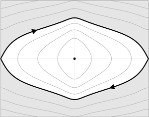
Notation and set-up. We illustrate a model swimmer in Poiseuille flow, located at a transverse displacement  $y$ from the midline of the parabolic flow profile. The swimming direction
  $\theta$ is measured from the midline, with
  $\theta =0$ corresponding to downstream swimming.

Via the numerical explorations of Omori et al. (Reference Omori, Kikuchi, Schmitz, Pavlovic, Chuang and Ishikawa2022), this model is noted to give rise to a range of complex, long-time behaviours, perhaps the most remarkable of which is conditional convergence towards a central upstream-facing configuration. In this study, we will aim to analytically uncover the driving factors behind these long-time dynamics. Via a multiple-scale asymptotic analysis (Bender & Orszag Reference Bender and Orszag1999), as recently applied to similar models of swimming (Gaffney et al. Reference Gaffney, Dalwadi, Moreau, Ishimoto and Walker2022; Ma, Pujara & Thiffeault Reference Ma, Pujara and Thiffeault2022; Walker et al. Reference Walker, Ishimoto, Gaffney, Moreau and Dalwadi2022), we will show how the effective swimmer behaviour can be captured by a Hamiltonian-like quantity, whose slow evolution accurately encodes the long-time trends of behaviour noted by Omori et al. (Reference Omori, Kikuchi, Schmitz, Pavlovic, Chuang and Ishikawa2022). Further, we will identify a markedly simple relation between the eventual behaviour of the swimmer and its oscillating speed and shape, enabling the deduction of long-time dynamics through the calculation of a single swimmer-dependent constant.
2. Direct asymptotic analysis
The time scales present in the model of Omori et al. (Reference Omori, Kikuchi, Schmitz, Pavlovic, Chuang and Ishikawa2022) are best identified through a change of variable. Defining  $z(t) := y(t)/\omega ^{1/2}$, the system reads
 $$\begin{gather} \frac{\mathrm{d}{z}}{\mathrm{d}{t}} = \omega^{1/2}u(\omega t)\sin{\theta}, \end{gather}$$
 $$\begin{gather}\frac{\mathrm{d}{\theta}}{\mathrm{d}{t}} = \gamma \omega^{1/2}z (1 - B(\omega t)\cos{2\theta}). \end{gather}$$
This suggests a natural fast time scale  $T := \omega t$, that of the oscillating swimmer speed and shape. Additionally,
  $O({1})$ oscillations of
  $u$ and
  $B$ in (2.1) drive
  $O({1})$ changes in
  $z$ and
  $\theta$ over an intermediate time scale of
  $t=O({\omega ^{-1/2}})$. We will later see that these changes correspond to quasi-periodic orbits of the swimmer in the flow, quantifying motion on this time scale via
  $\tau := \omega ^{1/2}t$. In addition to the two time scales
  $T$ and
  $\tau$ evident from this system of equations, Omori et al. (Reference Omori, Kikuchi, Schmitz, Pavlovic, Chuang and Ishikawa2022) observed behavioural changes over longer time scales, with
  $t=O({1})$. Hence, we expect the system to evolve on three separated time scales, corresponding to
  $T$,
$T$,  $\tau$ and
  $t$ each being
  $O({1})$. Our overarching aim is to characterise and understand the behaviours of the system over the time scale
  $t = O({1})$.
To this end, we conduct a multiple-scale analysis and formally write  $z(t) = z(T,\tau,t)$ and
  $\theta (t) = \theta (T,\tau,t)$, treating each time variable as independent (Bender & Orszag Reference Bender and Orszag1999). This transforms the proper time derivative via
 \begin{equation} \frac{\mathrm{d}{}}{\mathrm{d}{t}} \mapsto \omega\frac{\partial {}}{\partial {T}} + \omega^{1/2}\frac{\partial {}}{\partial {\tau}} + \frac{\partial {}}{\partial {t}}, \end{equation}
which transforms (2.1) into the system of partial differential equations
 $$\begin{gather} \omega z_T + \omega^{1/2}z_{\tau} + z_t = \omega^{1/2} u(T)\sin{\theta}, \end{gather}$$
 $$\begin{gather}\omega\theta_{T} + \omega^{1/2}\theta_{\tau} + \theta_{t} = \omega^{1/2}\gamma z (1 - B(T)\cos{2\theta}). \end{gather}$$
Here and hereafter, subscripts for  $t$,
$t$,  $\tau$ and
  $T$ denote partial derivatives. We will later remove the extra degrees of freedom that we have introduced by imposing periodicity of the dynamics in the intermediate and fast variables
  $\tau$ and
  $T$. Expanding
  $z$ and
  $\theta$ in powers of
  $\omega ^{-1/2}$ as
  $z \sim z_0 + \omega ^{-1/2}z_1 + \omega ^{-1}z_2 + \cdots$ and
  $\theta \sim \theta _0 + \omega ^{-1/2}\theta _1 + \omega ^{-1}\theta _2 + \cdots$, we obtain the
  $O({\omega })$ balance
 \begin{equation} z_{0T} = 0, \quad \theta_{0T} = 0, \end{equation}
so that  $z_0=z_0(\tau,t)$ and
  $\theta _0=\theta _0(\tau,t)$ are independent of
  $T$. To determine how
  $z_0$ and
  $\theta _0$ depend on
  $\tau$ and
  $t$, we must proceed to higher asymptotic orders.
We next consider the balance of  $O({\omega ^{1/2}})$ terms in (2.3), which reads
 $$\begin{gather} z_{1T} + z_{0\tau} = u(T)\sin{\theta_0}, \end{gather}$$
 $$\begin{gather}\theta_{1T} + \theta_{0\tau} = \gamma z_0(1 - B(T)\cos{2\theta_0}). \end{gather}$$
The Fredholm solvability condition for (2.5) is equivalent to averaging over a period in  $T$ and enforcing
  $T$-periodicity of
  $z_1$ and
  $\theta _1$. Introducing the averaging operator
  $\langle {\,{\cdot }\,} \rangle$, defined via its action on functions
  $v(T,\tau,t)$ via
 \begin{equation} \langle {v} \rangle(\tau,t) := \int_0^{1} v(T,\tau,t)\,\mathrm{d}{T}, \end{equation}
we obtain the averaged equations
 $$\begin{gather} z_{0\tau} = \langle {u} \rangle\sin{\theta_0}, \end{gather}$$
 $$\begin{gather}\theta_{0\tau} = \gamma z_0(1 - \langle {B} \rangle\cos{2\theta_0}), \end{gather}$$
where  $\langle {u} \rangle$ and
  $\langle {B} \rangle$ are the averages of
  $u(T)$ and
  $B(T)$, respectively, representing the average speed and shape of the model swimmer. In particular,
  $\langle {u} \rangle$ and
  $\langle {B} \rangle$ are constant, with the dynamics being rendered trivial if
  $\langle {u} \rangle =0$; we exclude this case from our analysis and henceforth take
  $\langle {u} \rangle >0$ without further loss of generality (the mapping
  $\theta \mapsto \theta +{\rm \pi}$ transforms
  $\langle {u} \rangle <0$ into the positive case). We will also assume that
  $\vert {\langle {B} \rangle } \vert <1$, which imposes only a minimal restriction on the admissible swimmer shapes, since
  $\vert {B} \vert \geq 1$ is typically associated with objects of exceedingly large aspect ratio (Bretherton Reference Bretherton1962).
Of particular note, if viewed as a system of ODEs in  $\tau$, the system of (2.7) corresponds precisely to the original dynamical system of (2.1), suitably scaled, but with the time-varying speed and shape parameters replaced by their averages. We will shortly return to these equations and explore the ramifications of this observation in detail, in particular noting the existence of a Hamiltonian-like quantity, but first complete our analysis of the
  $O({\omega ^{1/2}})$ problem to determine the form of
  $z_1$ and
  $\theta _1$ for later convenience.
Without solving (2.7), we can deduce the form of  $z_1$ and
  $\theta _1$ by substituting (2.7) into (2.5), yielding the simplified system
 $$\begin{gather} z_{1T} = [u(T) - \langle {u} \rangle]\sin{\theta_0}, \end{gather}$$
 $$\begin{gather}\theta_{1T} ={-}\gamma z_0[B(T) - \langle {B} \rangle]\cos{2\theta_0}. \end{gather}$$
Integrating (2.8) in  $T$, recalling that
  $z_0$ and
  $\theta _0$ are independent of
  $T$, yields the solution
 $$\begin{gather} z_1 = {I_u}(T)\sin{\theta_0} + \bar{z}_1(\tau,t), \end{gather}$$
 $$\begin{gather}\theta_1 ={-}\gamma z_0{I_B}(T)\cos{2\theta_0} + \bar{\theta}_1(\tau,t), \end{gather}$$
where  $\bar {z}_1$ and
  $\bar {\theta }_1$ are functions of
  $\tau$ and
  $t$, undetermined at this order, and we define
 \begin{equation} {I_u}(T) := \int_0^{T} [u(\tilde{T}) - \langle {u} \rangle] \,\mathrm{d}{\tilde{T}}, \quad {I_B}(T) := \int_0^{T} [B(\tilde{T}) - \langle {B} \rangle] \,\mathrm{d}{\tilde{T}}. \end{equation}
Noting that  ${I_u}(T)$ and
  ${I_B}(T)$ are
  $T$-periodic with period one, it follows that
  $z_1$ and
  $\theta _1$ are
  $T$-periodic with the same period.
In principle, one could proceed to the next asymptotic order to determine how  $z_0$ and
  $\theta _0$ evolve in
  $t$ through the derivation of an additional solvability condition. However, here, this procedure would be complicated by the absence of an explicit solution to the nonlinear system of equations (2.7), compounded by the potentially
  $t$-dependent period of the solution, which would require using the generalised method of Kuzmak (Reference Kuzmak1959). To circumvent this difficulty, we instead turn our attention back to (2.7), seeking further understanding of the leading-order dynamics over the intermediate time scale
  $\tau$.
3. A Hamiltonian-like quantity
If treated as a system of ODEs, we noted that (2.7) closely resembles the original swimming problem, with averages taking the place of oscillatory swimming speeds and swimmer shapes. In fact, the equivalent ODE problem has been extensively studied, with Zöttl & Stark (Reference Zöttl and Stark2013) thoroughly exploring this dynamical system and identifying a Hamiltonian-like constant of motion. Motivated by their study, we identify an analogous first integral of (2.7):
 \begin{equation} H_0(t) := \frac{\gamma}{2\langle {u} \rangle}z_0^{2} + g(\theta_0), \end{equation}
for  $H_0(t)\in [g({\rm \pi} ),\infty )$, where, for
  $\langle {B} \rangle \in (-1,1)$,
 \begin{equation} g(\theta_0) := \frac{\operatorname{arctanh}{\left(\sqrt{\dfrac{2\langle {B} \rangle}{1 +\langle {B} \rangle}}\cos{\theta_0}\right)}}{\sqrt{2\langle {B} \rangle(1+\langle {B} \rangle)}}, \quad g'(\theta_0) ={-}\frac{\sin{\theta_0}}{1 - \langle {B} \rangle\cos{2\theta_0}}, \end{equation}
taking the appropriate limits and branches where required. As  $H_0(t)$ is effectively a constant of motion over the intermediate time scale
  $\tau$, (3.1) demonstrates that solutions to (2.7) are closed orbits in
  $z_0$–
 $\theta _0$ phase space over this time scale, with
  $\theta _0$ appropriately understood to be taken modulo
  $2{\rm \pi}$.
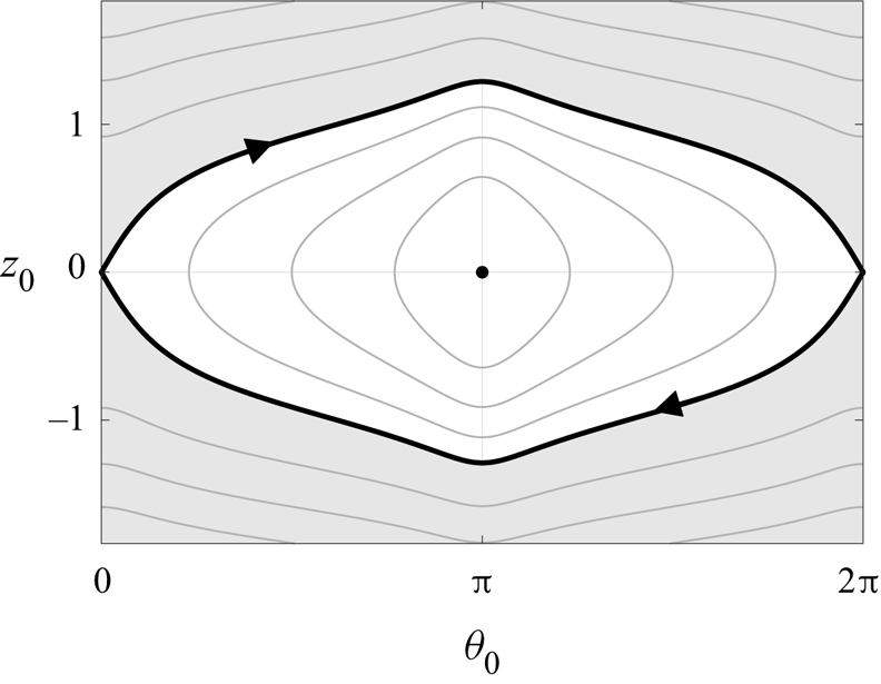
We illustrate this phase space in figure 2, equivalent to the plot of Zöttl & Stark (Reference Zöttl and Stark2013, figure 2b). In particular, it is helpful to emphasise the two distinct behavioural regimes on this time scale: (1) endless tumbling, where the swimmer does not cross  $z_0=0$ and
  $\theta _0$ varies monotonically; and (2) periodic swinging, where the swimmer repeatedly crosses the midline of the flow and
  $\theta _0$ oscillates between two values,
  $\theta _0\in [\theta _{{min}},\theta _{{max}}]$, readily computed from (3.1). The separating trajectory passes through
  $(z_0,\theta _0)=(0,0)$ and corresponds to
  $H_0=g(0)$. Here,
  $H_0 > g(0)$ corresponds to tumbling, shaded grey in figure 2, and
  $H_0 < g(0)$ corresponds to swinging. Of note, the period of these dynamics over the intermediate time scale, which we denote by
  ${P_{\tau }}$, depends non-trivially on
  $H_0$.
Phase portrait of motion on the intermediate time scale  $\tau$. Solutions of (3.1) are closed orbits in the
  $z_0$–
 $\theta _0$ plane for constant
  $H_0$, symmetric in both
  $z_0=0$ and
  $\theta _0={\rm \pi}$. Solutions in the shaded region, where
  $H_0 > g(0)$, do not cross
  $z_0=0$, corresponding to tumbling motion and monotonic evolution of
  $\theta _0$. Trajectories with
  $H_0 < g(0)$ instead exhibit swinging motion, with
  $\theta _0$ oscillating between two values. The black contour
  $H_0 = g(0)$ separates these regimes, with the direction of motion in the phase plane indicated by arrowheads, recalling that
  $\gamma \geq 0$. The point
  $(z_0,\theta _0)=(0,{\rm \pi} )$ corresponds to rheotaxis, with
  $H_0=g({\rm \pi} )$.
We can identify these dynamics with those reported both numerically and experimentally by Omori et al. (Reference Omori, Kikuchi, Schmitz, Pavlovic, Chuang and Ishikawa2022). In particular, as  $H_0(t)$ approaches its minimum of
  $g({\rm \pi} )$, the trajectory in the phase space approaches a single point,
  $(z_0,\theta _0)=(0,{\rm \pi} )$, corresponding to a swimmer that is directed upstream on the midline of the flow. This is precisely the so-called rheotactic behaviour observed by Omori et al. (Reference Omori, Kikuchi, Schmitz, Pavlovic, Chuang and Ishikawa2022), which they noted as the long-time behaviour of (1.1) for particular definitions of
  $u(T)$ and
  $B(T)$, corresponding also to the experimentally determined behaviours of Chlamydomonas in channel flow. This agreement suggests that the long-time dynamics of the full system may be captured by the evolution of the Hamiltonian-like quantity
  $H_0(t)$.
In order to examine this evolution, we consider the dynamics of the following Hamiltonian-like expression:
 \begin{equation} H(t) := \frac{\gamma}{2\langle {u} \rangle}z^{2} + g(\theta). \end{equation}
Taking the proper time derivative of (3.3) and inserting (2.1) yields
 \begin{equation} \frac{\mathrm{d}{H}}{\mathrm{d}{t}} = \gamma\omega^{1/2} z \sin{\theta} \left[\frac{u(T)}{\langle {u} \rangle} - \frac{1 - B(T)\cos{2\theta}}{1 - \langle {B} \rangle\cos{2\theta}}\right]. \end{equation}
Transforming the time derivative following (2.2), we then insert our expansions of  $z$ and
  $\theta$ into (3.4), noting that
  $H$ is equal to
  $H_0$ at leading order. Expanding
  $H\sim H_0 + \omega ^{-1/2}H_1 + \omega ^{-1}H_2+\cdots$, the balance at
  $O({\omega })$ is simply
  $H_{0T}=0$, so we deduce that
  $H_0=H_0(\tau,t)$, as expected. At
  $O({\omega ^{1/2}})$, we have
 \begin{equation} H_{1T} + H_{0\tau} = \gamma z_0\sin{\theta_0}\left[\frac{u(T)}{\langle {u} \rangle} - \frac{1 - B(T)\cos{2\theta_0}}{1 - \langle {B} \rangle\cos{2\theta_0}}\right]. \end{equation}
Averaging over the fast time scale  $T$, equivalent to applying the Fredholm solvability condition, we immediately see that the term in square brackets vanishes, so that
  $H_{0\tau } = 0$ and
  $H_0 = H_0(t)$ is also independent of
  $\tau$, as expected.
Finally, we consider the  $O({1})$ terms in (3.4), which may be stated as
 \begin{equation} H_{2T} + H_{1\tau} + H_{0t} = h(T,\tau,t), \end{equation}
where
 \begin{align} h(T,\tau,t) & := \gamma (z_0\theta_1 + z_1\sin{\theta_0})\left[\frac{u(T)}{\langle {u} \rangle} - \frac{1 - B(T)\cos{2\theta_0}}{1 - \langle {B} \rangle\cos{2\theta_0}}\right]\nonumber\\ & \quad - \frac{2\gamma z_0\theta_1 \sin{\theta_0}\sin{2\theta_0}}{(1-\langle {B} \rangle\cos{2\theta_0})^{2}} [B(T) - \langle {B} \rangle], \end{align}
and we note that the expressions in the square brackets each average to zero over a period in  $T$. Inserting our expressions for
  $z_1$ and
  $\theta _1$ from (2.9), we have
 \begin{align} h(T,\tau,t) & = \gamma(\sin^{2}{\theta_0}\,{I_u}(T) - \gamma z_0^{2} \cos{\theta_0}\cos{2\theta_0}\,{I_B}(T)) \left[\frac{u(T)}{\langle {u} \rangle} - \frac{1 - B(T)\cos{2\theta_0}}{1 - \langle {B} \rangle\cos{2\theta_0}}\right]\nonumber\\ &\quad + \frac{\gamma^{2} z_0^{2}\sin{\theta_0}\sin{2\theta_0} \cos{2\theta_0}}{(1-\langle {B} \rangle\cos{2\theta_0})^{2}}{I_B}(T)(B(T) - \langle {B} \rangle) + [\,{\cdot}\,], \end{align}
with  $[\,{\cdot }\,]$ encompassing terms that have zero fast-time-scale average, which here are those involving
  $\bar {z}_1$ and
  $\bar {\theta }_1$. It is also helpful to note that
  $2{I_B}(T)(B(T) - \langle {B} \rangle )=({I_B}^{2})_T$, so that
  $\langle {{I_B}(B - \langle{B}\rangle)} \rangle =0$ by the periodicity of
  ${I_B}$. Hence, the entire second line of (3.8) will vanish when averaged over a period in
  $T$. Averaging over
  $T$ and noting the further relations
  $\langle {{I_B}B} \rangle =\langle {{I_B}\langle{B}\rangle} \rangle$,
 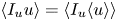 $\langle {{I_u}u} \rangle =\langle {{I_u}\langle{u}\rangle} \rangle$, and
 \begin{equation} ({I_u}{I_B})_T = {I_u}(T)(B(T)-\langle {B} \rangle) + {I_B}(T)(u(T)-\langle {u} \rangle), \end{equation}
the fast-time-scale average of  $h$ is simply
 \begin{equation} \langle {h} \rangle = \gamma \cos{2\theta_0}\left(\frac{\gamma}{\langle {u} \rangle}z_0^{2}\cos{\theta_0} +\frac{\sin^{2}{\theta_0}}{1 - \langle {B} \rangle\cos{2\theta_0}}\right) \underbrace{\langle {{I_u}(B - \langle{B}\rangle)} \rangle}_{W}, \end{equation}
where  $W :=\langle {{I_u}(B - \langle{B}\rangle)} \rangle$ is constant.
Thus, averaging (3.6) over a period in  $T$ and then over a period in
  $\tau$ (here, noting that
  $H_0$ is independent of
  $\tau$, we can naively average over a single oscillation in
  $\tau$, despite the
  $t$ dependence of
  ${P_{\tau }}$, which would otherwise require the method of Kuzmak (Reference Kuzmak1959)) yields the long-time evolution equation
 \begin{equation} \frac{\mathrm{d}{H_0}}{\mathrm{d}{t}} = \gamma f(H_0) W, \end{equation}
where
 \begin{equation} f(H_0) := \frac{1}{{P_{\tau}}}\int_0^{{P_{\tau}}} \cos{2\theta_0}\left(\frac{\gamma}{\langle {u} \rangle}z_0^{2}\cos{\theta_0} +\frac{\sin^{2}{\theta_0}}{1 - \langle {B} \rangle\cos{2\theta_0}}\right)\,\mathrm{d}{\tau}, \end{equation}
recalling that  ${P_{\tau }}$ denotes the period of the oscillatory dynamics in
  $\tau$ and
  $H_0$ is independent of
  $\tau$ and
  $T$. Notably, the integrand of (3.12) depends on the swimmer's speed and shape only via their fast-time averages
  $\langle {u} \rangle$ and
  $\langle {B} \rangle$. Therefore, all of the information encoding the dynamic variation of
  $u$ and
  $B$ about their mean is solely contained within the swimmer-dependent constant
  $W$. Of particular note, if either
  $u$ or
  $B$ is constant, then
  $W=0$ and, hence,
  $\mathrm {d}H_0/\mathrm {d}{t}=0$, so that there is no long-time drift of
  $H_0$. This analytically verifies the numerical observations of Omori et al. (Reference Omori, Kikuchi, Schmitz, Pavlovic, Chuang and Ishikawa2022), who concluded that oscillations in both swimmer speed and shape were required to modify long-time behaviour.
Having reduced the dynamics to the one-dimensional autonomous dynamical system of (3.11), notably independent of  $\omega$, it remains to understand
  $f(H_0)$, the average of a particular function of
  $z_0$ and
  $\theta _0$ over a period in
  $\tau$, which we illustrate in figure 3. In the Appendix, we analytically demonstrate that
  $f(H_0)\leq 0$ for all
  $H_0$, in agreement with figure 3. Hence, the sign of (3.11) is determined by
  $W$, which depends only on the dynamics of
  $u$ and
  $B$ over a single oscillation. Strictly, there is a higher-order problem to be solved close to
  $H_0=g(0)$, evidenced by the cusp-like profile in figure 3, with
  ${P_{\tau }}\rightarrow \infty$ and
  $f(H_0)\rightarrow 0$ as
  $H_0\rightarrow g(0)$. However, noting that
  $f(H_0)<0$ either side of
  $H_0=g(0)$, this point is half-stable in the context of (3.11) (Strogatz Reference Strogatz2018), so that it is unstable in practice and does not materially impact on the evolving dynamics.
Exemplifying  $f(H_0)$. We plot an example
  $f(H_0)$, as defined in (3.12) and computed numerically, for a range of
  $H_0$. The non-positivity of
  $f(H_0)$ is immediately evident, with
  $f\rightarrow 0$ from below as
  $H_0\rightarrow g({\rm \pi} )$ or
  $H_0\rightarrow g(0)$. As noted in the main text,
  $f$ is undefined at
  $H_0=g(0)$, which we indicate with a hollow circle, but this point is readily seen to be half-stable in the context of the dynamical system of (3.11), so has negligible impact on the dynamics in practice. Here, we have fixed
  $\gamma =1$,
  $\langle {u} \rangle =1$ and
  $\langle {B} \rangle =0.5$. The shaded region corresponds to tumbling dynamics.

Thus, the fixed point at  $H_0=g({\rm \pi} )$, corresponding to the rheotactic configuration
  $(z_0,\theta _0)=(0,{\rm \pi} )$, is globally stable if
  $W>0$ and unstable if
  $W<0$. Hence, rheotaxis is the globally emergent behaviour at leading order if
  $W>0$, whilst endless tumbling arises if
  $W<0$.
4. Summary and conclusions
Our analysis allows us to characterise the long-time behaviour of a swimmer in Poiseuille flow via the computation of a simple quantity,  $W$, defined in (3.10) and dependent only on the dynamics of the speed
  $u$ and the shape parameter
  $B$ of the swimmer over a single oscillation. In particular, we find that the long-time behaviours take one of three possible forms, given in terms of the leading-order Hamiltonian-like quantity
  $H_0$ of (3.1): (1) endless tumbling at increasing distance from the midline of the flow (
 $H_0\rightarrow \infty$); (2) preserved initial behaviour of the swimmer (
 $H_0 = H_0(0$)); or (3) convergence to upstream rheotaxis, where the swimmer is situated at the midline of the flow (
 $H_0\rightarrow g({\rm \pi} )$). We find that the drift towards these long-time regimes is caused by the delicate higher-order interactions in the system. Specifically, the nonlinear interaction between the small
  $O({\omega ^{-1/2}})$ variations from the leading-order system over the fast time scale
  $t = O(\omega^{-1})$ gives rise to the significant
  $O({1})$ effect over the slow time scale
  $t = O({1})$.
In the context of Omori et al. (Reference Omori, Kikuchi, Schmitz, Pavlovic, Chuang and Ishikawa2022), where  $u(T) = \alpha + \beta \sin (2{\rm \pi} T)$ and
  $B(T)=\delta + \mu \sin (2{\rm \pi} T+\lambda )$, we note that in-phase oscillations with
  $\lambda \in \{n{\rm \pi} \mid n\in \mathbb {Z}\}$ immediately lead to
  $W=0$, corresponding to case (2) above. Any other values of
  $\lambda$ lead to
  $W\neq 0$ (with maximal magnitude for
  $\lambda \in \{{\rm \pi} /2 + n{\rm \pi} \mid n\in \mathbb {Z}\}$) and long-term evolution of the swimmer behaviour. Notably, shifting
  $\lambda$ by
  ${\rm \pi}$ results in a precise reversal of the sign of
  $W$ and a corresponding reversal of the sign of
  $\mathrm {d}H_0/\mathrm {d}t$. Hence, this shift in phase will precisely flip the fate of the swimmer, with rheotaxis being replaced by tumbling, or vice versa. Concretely, if
  $\beta \mu >0$, then
  $\lambda \in (0,{\rm \pi} )$ results in tumbling, whilst
  $\lambda \in ({\rm \pi},2{\rm \pi} )$ gives rise to rheotaxis. Further, our analysis predicts that swimmers having either
  $u$ or
  $B$ constant will not undergo a similar drift over
  $t=O({1})$ at leading order. In particular, this highlights that rigid externally driven swimmers and Janus particles, associated with constant
  $B$, would differ fundamentally in their long-time behaviour from shape-changing swimmers with dynamically varying
  $B$.
$B$.
In support of our asymptotic analysis, we present three numerical examples in figure 4, approximating  $f(H_0)$ with quadrature using the easily obtained numerical solution of the simple ODE system of (2.7) in
  $\tau$ for fixed
  $H_0(t)$. In figure 4(a), we compare the asymptotic and full numerical solutions through the evolution of
  $H$, adopting the sinusoidal model of Omori et al. (Reference Omori, Kikuchi, Schmitz, Pavlovic, Chuang and Ishikawa2022) and demonstrating excellent agreement between the solutions. This numerical validation spans the distinct dynamical regimes of tumbling and swinging, with different values of the phase shift
  $\lambda$ giving rise to distinct behaviours from otherwise identical initial conditions. Figure 4(b) captures a transition between behaviours, as observed by Omori et al. (Reference Omori, Kikuchi, Schmitz, Pavlovic, Chuang and Ishikawa2022) for
  $\lambda =6{\rm \pi} /5$, where we have predicted the bounds of
  $z$ oscillations by combining the solution of (3.11) with (3.1) evaluated at
  $\theta _0=\theta _{{min}}$ and
  $\theta _0={\rm \pi}$. We anticipate that similar calculations may be used to predict collisions between swimmers and channel boundaries in related experimental set-ups, though theoretical consideration of boundary effects in future work is warranted and may complicate analysis. A promising direction for such an exploration is the augmentation of the model of Zöttl & Stark (Reference Zöttl and Stark2012) with the effects of an oscillatory swimming speed and swimmer shape, equivalent to extending the studied model of Omori et al. (Reference Omori, Kikuchi, Schmitz, Pavlovic, Chuang and Ishikawa2022) to a confined geometry.
Numerical validation. (a) The value of  $H$, as computed from the full numerical solution of (2.1) and the approximation of (3.11), shown as blue and black curves, respectively, for three phase shifts
  $\lambda \in \{4{\rm \pi} /5,{\rm \pi},6{\rm \pi} /5\}$. Small, rapid oscillations in the full numerical solution are visible in the inset. (b) The asymptotically predicted bounds of
  $z$ oscillations for
  $\lambda =6{\rm \pi} /5$ are shown as black curves, with the rapidly oscillating full solution shown in blue, highlighting excellent agreement even when the full solution transitions from tumbling dynamics towards rheotactic behaviour. Here, we have taken
  $(\alpha,\beta,\delta,\mu )=(1,0.5,0.32,0.3)$ and
  $\lambda \in \{4{\rm \pi} /5,{\rm \pi},6{\rm \pi} /5\}$ in the sinusoidal model of Omori et al. (Reference Omori, Kikuchi, Schmitz, Pavlovic, Chuang and Ishikawa2022), fixing
  $\gamma =1$,
  $\omega =50$ and
  $(z,\theta )=(1,{\rm \pi} /4)$ initially. The shaded regions correspond to tumbling dynamics.

More generally, the study of long-time swimmer dynamics in other scenarios, such as extensional flows, merits further investigation via multiple-scale analysis, with the behaviours of microswimmers in flow having been the subject of extensive research interest since the early twentieth century, as summarised by Bretherton & Rothschild (Reference Bretherton and Rothschild1961). Recent examples of this include, but are not limited to, the works of Marcos et al. (Reference Marcos, Fu, Powers and Stocker2012), Miki & Clapham (Reference Miki and Clapham2013) and Uspal et al. (Reference Uspal, Popescu, Dietrich and Tasinkevych2015), which consider the rheotaxis of bacteria, spermatozoa and active particles, respectively. The study of microswimmers in flow has also recently been considered in the context of theoretical control and guidance (Walker et al. Reference Walker, Ishimoto, Wheeler and Gaffney2018; Moreau & Ishimoto Reference Moreau and Ishimoto2021; Moreau et al. Reference Moreau, Ishimoto, Gaffney and Walker2021), further motivating the development of our understanding of the potentially subtle interactions between swimmer shape, swimming speed and background flows.
In summary, an asymptotic (three-time-scale) multiple-scale analysis of the swimming model of Omori et al. (Reference Omori, Kikuchi, Schmitz, Pavlovic, Chuang and Ishikawa2022) has revealed a trichotomy of startlingly simple long-time behaviours, determined only by a single swimmer-specific constant of motion that may be readily computed a priori. This analysis, which complements the earlier works of Zöttl & Stark (Reference Zöttl and Stark2012, Reference Zöttl and Stark2014) and Junot et al. (Reference Junot, Figueroa-Morales, Darnige, Lindner, Soto, Auradou and Clément2019), confirms the numerical predictions of Omori et al. (Reference Omori, Kikuchi, Schmitz, Pavlovic, Chuang and Ishikawa2022), in agreement with their experimental observations of Chlamydomonas, and formally identifies the interacting oscillatory effects needed to elicit the eventual behaviours of endless tumbling and upstream rheotaxis in this model of swimming.
Acknowledgements
The computer code used in this study is available at https://gitlab.com/bjwalker/emergent-rheotaxis-in-Poiseuille-flow.
Funding
B.J.W. is supported by the Royal Commission for the Exhibition of 1851. K.I. acknowledges JSPS-KAKENHI for Young Researchers (grant no. 18K13456), JSPS-KAKENHI for Transformative Research Areas (grant no. 21H05309) and JST, PRESTO, Japan (grant no. JPMJPR1921). C.M. is supported by the Research Institute for Mathematical Sciences, an International Joint Usage/Research Center located at Kyoto University. M.P.D. is supported by the UK Engineering and Physical Sciences Research Council (grant no. EP/W032317/1).
Declaration of interests
The authors report no conflict of interest.
Appendix. Deducing the sign of  $f(H_0)$

Consider the integrand of (3.12). Recalling the evolution equations of  $z_0$ and
  $\theta _0$ on the intermediate time scale, given in (2.7), this can be written as
 \begin{equation} \frac{\cos{2\theta_0}}{\langle {u} \rangle(1 - \langle {B} \rangle\cos{2\theta_0})}(z_0\sin{\theta_0})_{\tau}. \end{equation}
Integrating by parts then yields
 \begin{equation} {P_{\tau}}f(H_0) = \int_0^{{P_{\tau}}}\frac{2z_0\sin{\theta_0} \sin{2\theta_0}}{\langle {u} \rangle(1-\langle {B} \rangle\cos{2\theta_0})^{2}} \theta_{0\tau}\,\mathrm{d}{\tau} = \int\frac{2z_0\sin{\theta_0} \sin{2\theta_0}}{\langle {u} \rangle(1-\langle {B} \rangle\cos{2\theta_0})^{2}}\,\mathrm{d}{\theta_0}, \end{equation}
with boundary terms vanishing due to periodicity. With reference to the phase diagram of figure 2, we note that we need only integrate in  $\theta _0$ from its minimum attained value up to
  ${\rm \pi}$, with both the integrand and the phase-space trajectory being symmetric about both
  $\theta _0={\rm \pi}$ and
  $z_0=0$. This corresponds to integrating over the branch of the trajectory in the upper-left quadrant of figure 2, with the true value of
  ${P_{\tau }}f(H_0)$ then being recovered by appropriate multiplication by 2 or 4, depending on whether the trajectory is one of tumbling or swinging. Hence, we consider the integral only over the range
  $\theta _0\in [\theta _{{min}},{\rm \pi} ]$, where
  $\theta _{{min}}\in [0,{\rm \pi} ]$ is the minimum value attained by
  $\theta _0$ over an orbit, as specified solely by
  $H_0(t)$.
In the upper-left quadrant of the phase plane,  $z_0$ is a non-negative increasing function of
  $\theta _0$, evident from (2.7a) and (3.1). In particular,
  $z_0(\theta _0 + {\rm \pi}/2)\geq z_0({\rm \pi} /2)$ for
  $\theta _0\in [0,{\rm \pi} /2]$. Further, the remaining combination of trigonometric terms in the integrand, denoted by
  $I(\theta _0)$ for brevity, satisfies
  $I(\theta _0)\geq 0$ and
  $I(\theta _0 + {\rm \pi}/2) = -I(\theta _0)$ for
  $\theta _0\in [0,{\rm \pi} /2]$. Hence, the integral is trivially negative for
  $\theta _{{min}}\in [{\rm \pi} /2,{\rm \pi} ]$, whilst for
  $\theta _{{min}}\in [0,{\rm \pi} /2]$ we have
 \begin{align} \int_{\theta_{{min}}}^{{\rm \pi} } z_0(\theta_0)I(\theta_0)\,\mathrm{d}{\theta_0} & = \int_{\theta_{{min}}}^{{\rm \pi} /2} z_0(\theta_0)I(\theta_0)\,\mathrm{d}{\theta_0} + \int_{{\rm \pi} /2}^{{\rm \pi} }z(\theta_0)I(\theta_0)\,\mathrm{d}{\theta_0} \nonumber\\ & \leq \int_{0}^{{\rm \pi} /2} z_0({\rm \pi} /2)I(\theta_0)\,\mathrm{d}{\theta_0} + \int_0^{{\rm \pi} /2}z_0(\theta_0 + {\rm \pi}/2)I(\theta_0 + {\rm \pi}/2)\,\mathrm{d}{\theta_0} \nonumber\\ & = \int_0^{{\rm \pi} /2}[z_0({\rm \pi} /2) - z_0(\theta_0 + {\rm \pi}/2)]I(\theta_0)\,\mathrm{d}{\theta_0} \leq 0. \end{align}
Hence,  ${P_{\tau }}f(H_0) \leq 0$, so that
  $f(H_0)\leq 0$ for all
  $H_0$. In particular, this equality is strict unless
  $H_0=g({\rm \pi} )$ or
  $H_0=g(0)$, which correspond to the degenerate rheotactic trajectory
  $(z_0,\theta _0)=(0,{\rm \pi} )$ and the separating trajectory that lies between tumbling and swinging behaviours in figure 2. As discussed in the main text, the case with
  $H_0=g(0)$ requires the consideration of a higher-order problem, though has negligible impact on the dynamics in practice.


 Open access