

INTRODUCTION
The Asian monsoon (AM) is characterized by the seasonal reversal of circulation between ocean and landmasses throughout Southeast Asia, resulting in pronounced hydroclimate seasonality in the affected regions. Stalagmite oxygen isotope ratio (δ18O) records from the AM realm have provided crucial information on past climate conditions in this densely populated region (e.g., Wang et al., Reference Wang, Cheng, Edwards, He, Kong, An, Wu, Kelly, Dykoski and Li2005; Cheng et al., Reference Cheng, Edwards, Sinha, Spötl, Yi, Chen and Kelly2016a; Eroglu et al., Reference Eroglu, McRobie, Ozken, Stemler, Wyrwoll, Breitenbach, Marwan and Kurths2016). Pronounced glacial-interglacial variations in AM strength are found to be strongly influenced by Northern Hemisphere summer insolation (Cheng et al., Reference Cheng, Edwards, Broecker, Denton, Kong, Wang, Zhang and Wang2009, Reference Cheng, Edwards, Sinha, Spötl, Yi, Chen and Kelly2016a; Kathayat et al., Reference Kathayat, Cheng, Sinha, Spötl, Edwards, Zhang and Li2016) and closely related to changes in the North Atlantic (Wang et al., Reference Wang, Cheng, Edwards, An, Wu, Shen and Dorale2001; Yuan et al., Reference Yuan, Cheng, Edwards, Dykoski, Kelly, Zhang and Qing2004). The AM is therefore a highly dynamic system susceptible to external and internal forcings, calling for precise paleoclimate reconstructions throughout monsoonal Asia to infer future developments under climate change scenarios.
The majority of precisely dated high-resolution reconstructions of past glacial-interglacial AM variation stem from Chinese caves, providing unprecedented insight into monsoonal dynamics over the past 640,000 yr (Cheng et al., Reference Cheng, Edwards, Sinha, Spötl, Yi, Chen and Kelly2016a). Information from the Indian subcontinent, particularly at high temporal resolution and chronological precision, is still relatively scarce over these time scales (e.g., Sinha et al., Reference Sinha, Cannariato, Stott, Li, You, Cheng, Edwards and Singh2005; Govil and Divakar Naidu, Reference Govil and Divakar Naidu2011; Zhisheng et al., Reference Zhisheng, Clemens, Shen, Qiang, Jin, Sun and Prell2011; Menzel et al., Reference Menzel, Gaye, Mishra, Anoop, Basavaiah, Marwan and Plessen2014; Kathayat et al., Reference Kathayat, Cheng, Sinha, Spötl, Edwards, Zhang and Li2016). The Indian summer monsoon (ISM) is the branch of the AM that delivers moisture from the Arabian Sea and Indian Ocean to the Indian subcontinent, as well as to the Arabian peninsula (Burns et al., Reference Burns, Fleitmann, Mudelsee, Neff, Matter and Mangini2002; Fleitmann et al., Reference Fleitmann, Burns, Mangini, Mudelsee, Kramers, Villa and Neff2007), and China (Zhisheng et al., Reference Zhisheng, Clemens, Shen, Qiang, Jin, Sun and Prell2011; Baker et al., Reference Baker, Sodemann, Baldini, Breitenbach, Johnson, van Hunen and Pingzhong2015). It delivers ~80% of the annual rainfall of these regions and dominates their hydrologic cycle (Sinha et al., Reference Sinha, Cannariato, Stott, Cheng, Edwards, Yadava, Ramesh and Singh2007, Breitenbach et al. Reference Breitenbach, Adkins, Meyer, Marwan, Kumar and Haug2010) (Fig. 1A).
(A) Map with summer climatological conditions in the broader study area. The location of Mawmluh Cave in northeastern India is indicated by the black dot. Other discussed cave locations are indicated by the gray dots and arrows (D, Dongge Cave; K, Kulishu Cave; Y, Yamen Cave). The dashed line indicates maximum northward extent of the Intertropical Convergence Zone (ITCZ), which drives monsoonal circulation. Brown arrows delineate dominant Indian summer monsoon (ISM) circulation patterns; Asian summer monsoon (ASM) winds are shown in green. (B) Map of Mawmluh Cave. Stalagmite MAW-6 was found broken in the West Stream (map courtesy of Daniel Gebauer). (C) Scan of cut and polished stalagmite MAW-6. (For interpretation of the references to color in this figure legend, the reader is referred to the web version of this article.)

Stalagmite δ18O is a widely applied proxy for monsoonal strength in Asia and is interpreted as reflecting the δ18O of precipitation (Breitenbach et al., Reference Breitenbach, Adkins, Meyer, Marwan, Kumar and Haug2010, Reference Breitenbach, Lechleitner, Meyer, Diengdoh, Mattey and Marwan2015; Pausata et al., Reference Pausata, Battisti, Nisancioglu and Bitz2011; Cheng et al., Reference Cheng, Spötl, Breitenbach, Sinha, Wassenburg, Jochum and Scholz2016b; Eroglu et al., Reference Eroglu, McRobie, Ozken, Stemler, Wyrwoll, Breitenbach, Marwan and Kurths2016). As the δ18O signal is governed by a multitude of factors, their relative importance at a specific location needs to be carefully assessed to correctly interpret paleoclimatic data. Isotopic composition of the moisture source, transport length, and the amount of precipitation at the site can all affect precipitation δ18O in monsoonal regions, and taken together, they provide information on monsoonal strength (Breitenbach et al., Reference Breitenbach, Adkins, Meyer, Marwan, Kumar and Haug2010; Baker et al., Reference Baker, Sodemann, Baldini, Breitenbach, Johnson, van Hunen and Pingzhong2015; Eroglu et al., Reference Eroglu, McRobie, Ozken, Stemler, Wyrwoll, Breitenbach, Marwan and Kurths2016). Cave monitoring efforts and simultaneous study of different stalagmite geochemical proxies in parallel often allow researchers to more clearly determine the controls on local climate conditions, leading to more accurate paleoclimate reconstructions (Baldini, Reference Baldini2010; Oster et al., Reference Oster, Montañez and Kelley2012; Breitenbach et al., Reference Breitenbach, Lechleitner, Meyer, Diengdoh, Mattey and Marwan2015; Baldini et al., Reference Baldini, Baldini, McElwaine, Frappier, Asmerom, Liu and Prufer2016; Cheng et al., Reference Cheng, Spötl, Breitenbach, Sinha, Wassenburg, Jochum and Scholz2016b). Stable carbon isotope ratios (δ13C) are routinely measured together with δ18O but have so far rarely been reported for records from monsoonal Asia. This is partly because of the more complicated and site-specific interpretation of stalagmite δ13C, which necessitates thorough understanding of the local conditions; δ13C can be influenced by vegetation composition (i.e., C3 vs. C4 plants), soil processes, open versus closed conditions in the karst during carbonate dissolution, and isotope fractionation in or above the cave (Fairchild and Baker, Reference Fairchild and Baker2012). However, carefully evaluated stalagmite δ13C time series can provide important climate information to supplement and extend the interpretation of δ18O records, often resulting in a more in-depth understanding of past climate conditions (Genty et al., Reference Genty, Blamart, Ouahdi, Gilmour, Baker, Jouzel and Van-Exter2003; Cosford et al., Reference Cosford, Qing, Mattey, Eglington and Zhang2009; Ridley et al., Reference Ridley, Asmerom, Baldini, Breitenbach, Aquino, Prufer and Culleton2015; Cheng et al., Reference Cheng, Spötl, Breitenbach, Sinha, Wassenburg, Jochum and Scholz2016b). Particularly interesting is the difference in spatial scale between both proxies: δ18O generally reflects large-scale atmospheric circulation processes (Breitenbach et al., Reference Breitenbach, Adkins, Meyer, Marwan, Kumar and Haug2010; Baker et al., Reference Baker, Sodemann, Baldini, Breitenbach, Johnson, van Hunen and Pingzhong2015), whereas δ13C is a proxy for local processes and is therefore more sensitive to changes at local to regional levels (Ridley et al., Reference Ridley, Asmerom, Baldini, Breitenbach, Aquino, Prufer and Culleton2015; Cheng et al., Reference Cheng, Spötl, Breitenbach, Sinha, Wassenburg, Jochum and Scholz2016b).
Here, we present new subdecadally resolved δ18O and δ13C data from a stalagmite from NE India that cover the interval of the last deglaciation and early Holocene (EH; ~16–6.5 ka). The last deglaciation was a period of rapid and substantial global climate change, driven by a ~3.5°C increase in global temperatures (Shakun et al., Reference Shakun, Clark, He, Marcott, Mix, Liu, Otto-Bliesner, Schmittner and Bard2012). This resulted in large-scale reorganizations of circulation and weather patterns globally, with important repercussions in monsoonal Asia (Dykoski et al., Reference Dykoski, Edwards, Cheng, Yuan, Cai, Zhang, Lin, Qing, An and Revenaugh2005; Cheng et al., Reference Cheng, Edwards, Broecker, Denton, Kong, Wang, Zhang and Wang2009; Ma et al., Reference Ma, Cheng, Tan, Edwards, Li, You, Duan, Wang and Kelly2012). This analysis follows long-term studies of the controls on precipitation δ18O (Breitenbach et al., Reference Breitenbach, Adkins, Meyer, Marwan, Kumar and Haug2010), as well as detailed cave microclimate monitoring schemes (Breitenbach et al., Reference Breitenbach, Lechleitner, Meyer, Diengdoh, Mattey and Marwan2015), which allow us to disentangle local and regional responses to climate change over the last deglaciation.
GEOGRAPHIC AND CLIMATOLOGICAL SETTING
Mawmluh Cave is located at 25.26°N, 91.88°E, 1320 m above sea level on the Meghalaya Plateau in NE India (Fig. 1). The cave developed in a Tertiary limestone butte at the southern fringe of the plateau (Ghosh et al., Reference Ghosh, Fallick, Paul and Potts2005; Gebauer, Reference Gebauer2008) and is today mainly covered by grassland. Mean annual air temperature inside the cave (18.5°C) is very similar to that recorded at the meteorological station Cherrapunji (17.4°C) and in the nearby Mawmluh village (19.1°C).
Hydroclimate in Meghalaya is extremely seasonal, with ~80% of annual precipitation falling during the ISM season (June–October; Breitenbach et al., Reference Breitenbach, Adkins, Meyer, Marwan, Kumar and Haug2010). The Meghalaya Plateau is the first morphological barrier for northward-moving moisture from the Bay of Bengal (BoB), inducing intense orographic rainfall. Thus, Meghalaya is a major water source for the Bangladesh plains, a region frequently flooded during summer—for example, in 1998, when ~60% of the country was inundated (Murata et al., Reference Murata, Terao, Hayashi, Asada and Matsumoto2008; Webster, Reference Webster2013). Despite having the highest rainfall amount in the world (Prokop and Walanus, Reference Prokop and Walanus2003), low retention capacity, because of the geologic conditions on the southern Meghalaya Plateau, results in frequent water shortage during the dry season (November–May).
MATERIALS AND METHODS
Stalagmite MAW-6
The 21-cm-long stalagmite MAW-6 was found broken in Mawmluh Cave in 2009, and its original position is known only approximately (Fig. 1). The stalagmite displays complex brown-gray color variations, with bands up to a few millimeters wide, but no annual laminations. At least three white layers can be discerned, which span from the growth axis toward the sides of the stalagmite. To verify the mineralogy in MAW-6, three samples were analyzed by X-ray diffraction (XRD) using a powder XRD diffractometer (Bruker, D8 Advance), equipped with a scintillation counter and an automatic sampler at ETH Zurich, Switzerland.
U-series dating and chronology development
After cutting the stalagmite lengthwise using a diamond stone saw, 24 U-series samples with weights between 88 and 311 mg were milled using an ethanol-cleaned stainless steel bit and subsequently analyzed by multicollector inductively coupled plasma mass spectrometry using a Thermo-Finnigan Neptune in the Minnesota isotope laboratory, University of Minnesota. The chemical procedures used to separate uranium and thorium for U-series dating are similar to those described in Edwards et al. (Reference Edwards, Chen and Wasserburg1987). Uranium and thorium isotopes were analyzed on the multiplier behind the retarding potential quadrupole in peak-jumping mode. Instrumental mass fractionation was determined by measurements of a 233U/236U spike. The detail techniques are similar to those described by Cheng et al. (Reference Cheng, Edwards, Hoff, Gallup, Richards and Asmerom2000, Reference Cheng, Edwards, Broecker, Denton, Kong, Wang, Zhang and Wang2009), and half-life values are those reported by Cheng et al. (Reference Cheng, Edwards, Shen, Polyak, Asmerom, Woodhead and Hellstrom2013).
The age model for MAW-6 was computed for each growth segment by applying a cubic interpolation procedure using the COPRA software (Breitenbach et al., Reference Breitenbach, Rehfeld, Goswami, Baldini, Ridley, Kennett and Prufer2012). COPRA computed 2000 ensemble realizations for both the δ18O and δ13C records, from which the median (i.e., the central age for a defined sample depth) was calculated. The uncertainty in the age model is defined by the 95% confidence intervals, derived using the ±2σ deviation from the median (Breitenbach et al., Reference Breitenbach, Rehfeld, Goswami, Baldini, Ridley, Kennett and Prufer2012).
Stable isotope analysis
One thousand and fifty samples for stable isotope analysis were milled continuously at 200 μm resolution using a semiautomated high-precision drill (Sherline 5400 Deluxe) at ETH Zurich. Nine Hendy tests were performed over the length of the stalagmite to look for signs of kinetic isotope fractionation effects and, if present, to evaluate potential changes in the intensity of kinetic fractionation through time (Supplementary Fig. 1). For this, carbonate samples were drilled point-wise along a single layer of the stalagmite using a 0.3-mm-diameter drill bit.
Samples were analyzed for δ18O and δ13C on a Delta V Plus mass spectrometer coupled to a ThermoFinnigan GasBench II carbonate preparation device at the Geological Institute, ETH Zurich (Breitenbach and Bernasconi, Reference Breitenbach and Bernasconi2011). An in-house carbonate standard (MS2), which is well linked to NBS19 (Breitenbach and Bernasconi, Reference Breitenbach and Bernasconi2011), was used to evaluate the runs. All values are expressed in per mil (‰) and referenced to the Vienna Pee Dee belemnite standard. The external standard deviation (1σ) for both δ18O and δ13C analyses on the carbonate is smaller than 0.07‰.
Because the MAW-6 record covers the period of the last deglaciation, the contribution of changes in both sea surface temperature (SST) and sea level because of the melting of continental ice sheets to stalagmite δ18O must be considered. To estimate this contribution, a linear interpolation of seawater δ18O values (δ18Oseawater) reconstructed from a sediment core from the BoB (Rashid et al., Reference Rashid, England, Thompson and Polyak2011) was performed to fit the MAW-6 data points. The δ18Oseawater record was subsequently subtracted from the measured δ18Ocalcite in MAW-6, to yield an ice-volume-corrected (δ18OIVC) record (Supplementary Fig. 2). It should be noted that this procedure can introduce artifacts, as the records are irregularly sampled, and the results should be interpreted with care.
Recurrence quantification analysis
To infer possible changes in the dynamic regime of the ISM between late glacial (LG) and EH conditions, we performed a statistical analysis considering the deterministic nature of the underlying process (the ISM), encoded by the recurrence properties of the δ18OIVC record. We use a measure of complexity, called recurrence determinism (DET), which is derived from a recurrence plot, a graphic, binary representation of pairs of times of similar values (actually states) within the time series (see Supplementary Materials for further details; Marwan et al., Reference Marwan, Romano, Thiel and Kurths2007; Ozken et al., Reference Ozken, Eroglu, Stemler, Marwan, Bagci and Kurths2015; Eroglu et al., Reference Eroglu, McRobie, Ozken, Stemler, Wyrwoll, Breitenbach, Marwan and Kurths2016). DET reveals high values for deterministic processes and regular (e.g., cyclic, periodic) variations, whereas more stochastic (i.e., random) dynamics lead to low DET values. Moreover, the recurrence analysis is combined with the preprocessing Transformation-Cost Time-Series (TACTS) technique that allows detrending regularization of irregularly sampled time series (see Supplementary Materials; Ozken et al., Reference Ozken, Eroglu, Stemler, Marwan, Bagci and Kurths2015).
The δ18OIVC record was divided into two periods, the LG period (16–13ka) and the EH (9–6.5ka), and the DET measures were calculated for both periods separately. A statistical test based on a bootstrap approach was performed to evaluate the significance of the variations in the DET measure. This test provides a cumulative probability distribution of DET measures corresponding to the null hypothesis that there is no change in the dynamics of the underlying climate process. From this test distribution, the upper 95% confidence limit can be defined.
RESULTS
Petrography and mineralogy
XRD analysis reveals that stalagmite MAW-6 consists of calcite. The white layers described previously were identified as dirt layers in the stalagmite. They are well visible at the fringes of the respective layers, and the stalagmite tip has been washed clean by impinging water droplets (Fig. 1C). The deposition of silty material on the stalagmite surface at these depths might indicate burial of MAW-6 by sediment redeposition in the cave, inhibiting further growth. Several buried stalagmites have been located in the cave (Supplementary Fig. 3), and sediment migration within the cave passage appears to be an important process during high-discharge events of the cave stream. However, caution must be applied with this interpretation because dirt layers can also originate from other processes, such as aerosol and dust deposition.
Age model
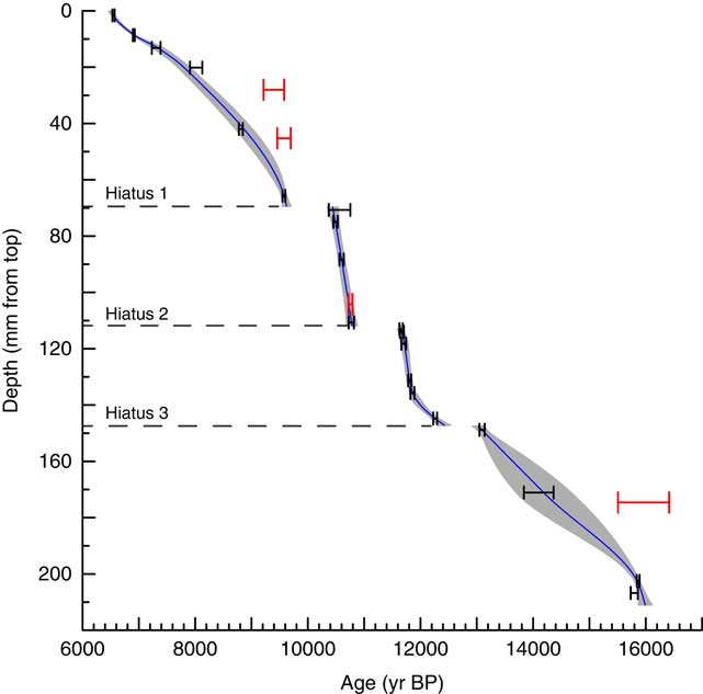
MAW-6 grew between ~16 and 6.5ka. The age model is based on 20 U-series dates, with analytical errors between ±16 and ±264 yr (Fig. 2, Table 1). Four dating samples contained high amounts of detrital thorium and were excluded from the final age model (shown in red in Fig. 2).
Age model of MAW-6 (constructed using cubic interpolation in COPRA). The median of the age model is shown in blue, with the 95% confidence intervals in light gray. The U-series ages used to construct the age model are shown in black, and the excluded ages are in red. Hiatuses are indicated by dashed black lines. (For interpretation of the references to color in this figure legend, the reader is referred to the web version of this article.)
U-series dating results for stalagmite MAW-6. The errors given are 2σ. Corrected 230Th ages assume the initial 230Th/232Th atomic ratio of 4.4 ± 2.2 × 10⁻⁶. Those are the values for a material at secular equilibrium, with the bulk earth 232Th/238U value of 3.8. The errors are arbitrarily assumed to be 50%. Values are indicated at one decimal place more than significant, to avoid rounding errors. Ages excluded from the final chronology are shown in italics.

a δ234U = ([234U/238U]activity − 1)×1000.
b BP stands for “before present” where the “present” is defined as the year AD 1950.
c δ234Uinitial was calculated based on 230Th age (T) (i.e., δ234Uinitial = δ234Umeasured × e λ234 × T ).
Three hiatuses were identified in the depth-age relationship, coinciding with the white dirt layers in the stalagmite. User-specified hiatus depths of 69.46, 111.86, and 147.26 mm from the stalagmite top allowed COPRA to split the age model construction into independent age models (before and after the hiatuses, respectively). This procedure yielded a segmented depth-age chronology for the stalagmite, with hiatuses at 10.4–9.6, 11.6–10.8, and 13–12.4ka. The details for the age-modeling procedure can be found in Breitenbach et al. (Reference Breitenbach, Rehfeld, Goswami, Baldini, Ridley, Kennett and Prufer2012).
Using the COPRA procedure, the age uncertainties of the MAW-6 record can be transferred from the age to the proxy domain (Breitenbach et al., Reference Breitenbach, Rehfeld, Goswami, Baldini, Ridley, Kennett and Prufer2012), which results in a 95% confidence interval of possible proxy values at a given point in time. As a consequence, it is not possible to determine the high-frequency variations within the bounds of the confidence interval (Fig. 3A). Comparative discussions with other paleoclimate records from the AM realm are therefore restricted to the median proxy values in MAW-6 derived from the COPRA Monte Carlo modeling and to long-term centennial changes. We still show the original MAW-6 isotope data for a tentative comparison with other available records in (see discussion), as this kind of uncertainty is common to all paleoclimate records.
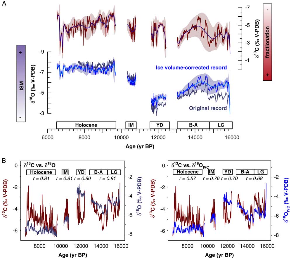
(color online) (A) δ18O and δ13C records with median and 95% confidence intervals. The time periods discussed in this study are indicated at the bottom of the figure (B-A, Bølling-Allerød; IM, intermediate period, 10.8–10.2ka; LG, late glacial; YD, Younger Dryas). Major controls on δ18O (Indian summer monsoon [ISM] strength) and δ13C (amount of in-cave fractionation as a result of cave air pCO2 and drip rate) are indicated by the bars. (B) Cross correlation between δ18O and ice-volume-corrected δ18O (δ18OIVC) versus δ13C, estimated using kernel-based cross correlation analysis (Rehfeld and Kurths, Reference Rehfeld and Kurths2014) with the toolbox NESTool (http://tocsy.pik-potsdam.de/nest.php). V-PDB, Vienna Pee Dee belemnite.
The MAW-6 δ18O and δ13C records
The δ18O profile varies from −8.3‰ to −2.8‰ (Fig. 3A), with heavier values found in the oldest part of the record (end of the last glacial period), and lighter values in the youngest part (the Holocene). Both, the Bølling-Allerød (B-A) interstadial period, beginning at ~14.5ka with −1.5‰ shift, and the Younger Dryas (YD), between 12.6 and 11.6ka and featuring the heaviest values of the entire record (approximately −3.5‰), are clearly demarcated. However, the exact beginning and the end of the YD in MAW-6 cannot be defined because the interval is bracketed by two hiatuses. The 850-yr-long hiatus that masks the end of the YD is followed by a substantial 4.5‰ decrease in δ18O, marking the transition into the Holocene (~9.6ka). This decrease occurs in two rapid stages, characterized by hiatuses, interrupted by an interval (~10.8–10.2ka) of relatively constant intermediate values (approximately −6.5‰). Lowest δ18O values (~ −8‰) are found during the EH (~9.6ka), slightly increasing toward the youngest part of the record. Our sea-level-corrected δ18OIVC record shows that ice volume and SST changes affect the isotope signature mainly before the YD, with only minor impacts during the Holocene, accounting for ~1/4 (1‰) of the shift between deglaciation and Holocene (Fig. 3A). We are therefore confident that the larger part (3‰) of the variation in δ18O during the deglaciation is attributable to changes in ISM strength. For the following discussion, only the δ18OIVC record is considered.
Compared with the δ18O profile, the δ13C profile is much more uniform, with variations ranging between −1.2‰ and −6.6‰ and without clear trends over time. The heaviest values are found during the early part of the record (LG/B-A, average −4‰). In contrast to δ18O, the YD period is characterized by slightly lighter values than during the LG/B-A section (average −4.3‰), whereas the transition into the Holocene leads to the most negative values (average −5.2‰ post ~9.6ka). The high-frequency variations in δ18O and δ13C are remarkably similar, but shifts in δ13C are generally much more pronounced than in δ18O. The similarity between the two records is also reflected by their high correlation (during all periods, r>0.55; Fig. 3B).
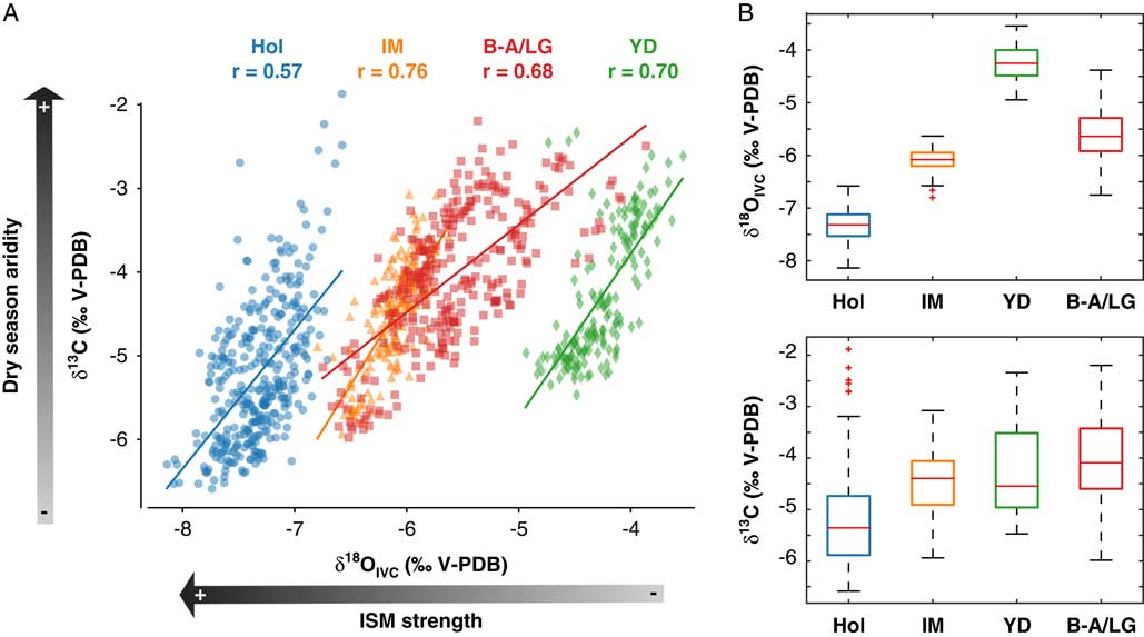
A cross plot of δ13C versus δ18OIVC reveals four distinct clusters (Fig. 4). These clusters are mainly influenced by the average δ18OIVC during the different periods; therefore, we distinguish Holocene, intermediate (10.8–10.2ka), YD, and B-A/LG clusters. The box plot representation of the data sets in Figure 4B allows the quantification of temporal and proxy-related differences. Although a clear distinction of the different time periods is apparent in the δ18OIVC data set, a much larger spread in δ13C values is found (Fig. 4B). The YD cluster is characterized by the heaviest δ18OIVC values of the entire record, whereas δ13C is slightly lighter than during the LG period. A trend toward progressively lighter δ18OIVC values is found between the YD, intermediate, and Holocene clusters, whereas intermediate δ13C values are slightly heavier than during the YD (Fig. 4B).
(A) δ13C versus ice-volume-corrected δ18O (δ18OIVC) relationship in stalagmite MAW-6. The record can be subdivided into clusters corresponding to different time periods: Holocene (Hol), intermediate (IM), Younger Dryas (YD), and Bølling-Allerød and late glacial (B-A/LG). All clusters show high degrees of correlation between δ13C and δ18OIVC, indicated by the corresponding r values (same values as in Fig. 3B). Arrows indicate the direction of the main forcings (dry season aridity and Indian summer monsoon [ISM] strength). (B) Boxplots for δ18OIVC and δ13C (top and bottom panels, respectively). Boxes are defined by the median (red line) and delimited by the first and third quartiles. Whiskers define the lowest and highest values within 1.5 times the interquartile range of the cluster. Outliers are indicated by red crosses. V-PDB, Vienna Pee Dee belemnite. (For interpretation of the references to color in this figure legend, the reader is referred to the web version of this article.)
The Hendy tests carried out throughout MAW-6 show evidence for kinetic fractionation during the YD and the LG period, whereas (near-) equilibrium conditions seem to have prevailed during the B-A and the Holocene (Supplementary Fig. 1). Kinetic effects are identified by strong correlations between δ18O and δ13C, as well as enrichment in the heavy isotopes with increasing distance from the growth axis (Hendy, Reference Hendy1971).
Determinism of the δ18O record
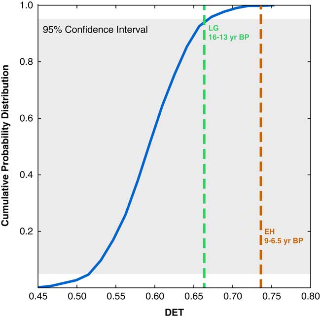
The analysis reveals distinctly different DET measures for the LG (DET = 0.663, inside the confidence interval) and the EH (DET = 0.736, outside the confidence interval). A high DET measure indicates a more predictable (i.e., a less chaotic) regime, whereas the opposite holds true for low DET measures.
DISCUSSION
Influence of karst processes on stalagmite stable isotopes in Mawmluh Cave
Karst processes at Mawmluh Cave are driven by the seasonal cycle in regional hydrology (Fig. 5). Precipitation δ18O becomes increasingly lighter during the ISM months and reaches the most negative values during the late and post-ISM (August–October) (Breitenbach et al., Reference Breitenbach, Adkins, Meyer, Marwan, Kumar and Haug2010). A direct amount effect can therefore be ruled out, as maximum precipitation occurs earlier in the ISM season (July–August). Instead, precipitation δ18O in Meghalaya is controlled by the following: (1) the travel distance of the air masses, which increases throughout the ISM season, promoting stronger Rayleigh fractionation during transport and lighter δ18O at the site (Breitenbach et al., Reference Breitenbach, Adkins, Meyer, Marwan, Kumar and Haug2010); (2) stronger contribution from isotopically depleted freshwater delivered to the BoB during the late ISM (Sengupta and Sarkar, Reference Sengupta and Sarkar2006; Singh et al., Reference Singh, Singh and Müller2007; Breitenbach et al., Reference Breitenbach, Adkins, Meyer, Marwan, Kumar and Haug2010); and (3) isotopic depletion of rainwater during large rainstorms (amount effect sensu Dansgaard, Reference Dansgaard1964) (Lawrence et al., Reference Lawrence, Gedzelman, Dexheimer, Cho, Carrie, Gasparini, Anderson, Bowman and Biggerstaff2004; Breitenbach et al., Reference Breitenbach, Adkins, Meyer, Marwan, Kumar and Haug2010; Baker et al., Reference Baker, Sodemann, Baldini, Breitenbach, Johnson, van Hunen and Pingzhong2015). These mechanisms all drive precipitation δ18O in the same direction, resulting in lighter δ18O during and after the ISM and heavier values during dry season months (Breitenbach et al., Reference Breitenbach, Lechleitner, Meyer, Diengdoh, Mattey and Marwan2015; Myers et al., Reference Myers, Oster, Sharp, Bennartz, Kelley, Covey and Breitenbach2015). At Mawmluh Cave, infiltration is strongly skewed toward the summer months, and consequently, drip water δ18O is biased toward the ISM season (Fig. 5). Still, a clear seasonal cycle in drip water δ18O is observed, with the lightest values occurring during the late ISM months, indicating rapid (<1 month) fluid transfer into the cave (Breitenbach et al., Reference Breitenbach, Lechleitner, Meyer, Diengdoh, Mattey and Marwan2015) (Fig. 5). Drip water (and stalagmite) δ18O at Mawmluh Cave can therefore be used as a reliable ISM strength proxy.
(color online) Schematic of the factors influencing isotope signals at Mawmluh Cave. Data are derived from monitoring studies at the cave site (Breitenbach et al., Reference Breitenbach, Lechleitner, Meyer, Diengdoh, Mattey and Marwan2015), and precipitation data are from the Indian Meteorological Department Station Cherrapunji. VSMOW, Vienna standard mean ocean water. PCP, prior calcite precipitation.
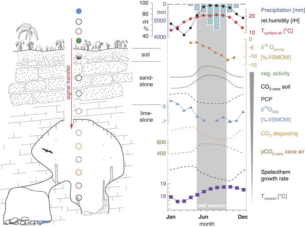
Drip water δ13C can be influenced by changes in vegetation type above the cave (C3 vs. C4 plants; Denniston et al., Reference Denniston, Gonzalez, Asmerom and Polyak2001), soil activity (Genty et al., Reference Genty, Blamart, Ghaleb, Plagnes, Causse, Bakalowicz and Zouari2006; Scholz et al., Reference Scholz, Frisia, Borsato, Spötl, Fohlmeister, Mudelsee, Miorandi and Mangini2012), bedrock dissolution and open versus closed system conditions in the karst (Genty et al., Reference Genty, Baker, Massault, Proctor, Gilmour, Pons-Branchu and Hamelin2001), and prior calcite precipitation Prior calcite precipitation is correct (PCP). and fractionation processes in the cave (Griffiths et al., Reference Griffiths, Fohlmeister, Drysdale, Hua, Johnson, Hellstrom, Gagan and Zhao2012; Ridley et al., Reference Ridley, Asmerom, Baldini, Breitenbach, Aquino, Prufer and Culleton2015). At Mawmluh Cave, precipitation and consequently vegetation and soil activity (microbial activity and root respiration) are at a maximum during the summer months (June–October), resulting in highest relative humidity and soil pCO2 during this period. The extremely high amounts of rainfall delivered at Mawmluh Cave during the ISM season (max. 13,472 mm between June and September; Breitenbach et al., Reference Breitenbach, Lechleitner, Meyer, Diengdoh, Mattey and Marwan2015) lead to waterlogging of the soil and karst overlying the cave (Breitenbach et al., Reference Breitenbach, Lechleitner, Meyer, Diengdoh, Mattey and Marwan2015), most likely resulting in more closed system conditions. Therefore, PCP in epikarst and cave is minimized (or even completely absent) during the ISM season. Strong seasonal variations in cave air pCO2 are observed as a consequence of seasonal ventilation changes (Breitenbach et al., Reference Breitenbach, Lechleitner, Meyer, Diengdoh, Mattey and Marwan2015) (Fig. 5). During the dry season months, low cave air pCO2 attributable to strongly reduced rainfall amount above the cave and intensified ventilation, leads to enhanced degassing of CO2 from the solution, enriching drip water in 13C (Breitenbach et al., Reference Breitenbach, Lechleitner, Meyer, Diengdoh, Mattey and Marwan2015). Moreover, open system conditions prevail in the overlying soil and karst, because of seasonal aridity, resulting in low soil activity (less input of isotopically light organic carbon to soil water) and promoting PCP (Fig. 5). All factors taken together, conditions during the dry season result in heavier drip water δ13C in Mawmluh Cave, whereas the opposite holds true for the ISM months. Drip water and stalagmite δ13C are therefore strongly influenced by effective infiltration in the soil and tightly connected to local climate conditions.
Interpretation of the MAW-6 isotope records
We find large variations in δ18OIVC in stalagmite MAW-6 over the period of the last deglaciation, with the heaviest values recorded during the LG period and the YD (Fig. 3). Considering the controls on precipitation and drip water δ18OIVC at Mawmluh Cave, we interpret the LG and YD portions of the record as periods of weaker/shorter ISM, accompanied by changes in the circulation regime (i.e., a more proximal moisture source), whereas stronger ISM and longer moisture transport paths prevailed during the B-A and the Holocene. Changes in both SST and sea level because of the melting of the continental ice sheets during the last deglaciation resulted in substantial alteration of the isotopic composition of the surface ocean water and also affected evaporation and convection from the sea surface (Gadgil, Reference Gadgil2003). The changes in the moisture source affect precipitation and stalagmite δ18O. In the BoB, the moisture source for the ISM, a ~3.2–3.5°C increase in SST between the last glacial maximum and the Holocene, and a +1.4°C SST shift between the YD and the Holocene have been documented (Rashid et al., Reference Rashid, Flower, Poore and Quinn2007, Reference Rashid, England, Thompson and Polyak2011; Govil and Divakar Naidu, Reference Govil and Divakar Naidu2011). In this region, additional depletion of seawater 18O occurred most likely because of freshening of the BoB by increased runoff from precipitation and glacier melt in the Himalaya and Tibet.
The millennial-scale average in MAW-6 δ13C shows much lower variability than δ18OIVC over the last deglaciation, but the centennial-scale variations are remarkably similar (Fig. 3). It is likely that changes in vegetation density and composition occurred between cold/dry glacial and warm/humid interglacial periods. However, vegetation changes above the cave as the primary cause for the high frequency variation in δ13C can probably be ruled out, as these would require longer time periods and would likely be more gradual than the rapid decadal-scale shifts we find in MAW-6. Karst processes—namely, PCP and kinetic fractionation in the cave—can best explain the observed variation in MAW-6 δ13C. We find heavier δ13C values during weak ISM periods, as identified in the δ18OIVC record, indicating enhanced PCP and kinetic fractionation stemming from drier summer and/or longer winter seasons. Periods of strong ISM, on the other hand, are characterized by lighter δ13C values, which is in line with more closed system conditions during the wet summers; higher cave air pCO2, which subdues kinetic fractionation; and more active vegetation and soil.
It is possible that kinetic processes affect stalagmite δ18O as well, precluding quantitative rainfall reconstructions, but still allowing qualitative interpretation of monsoon strength. In fact, kinetic fractionation would drive stalagmite δ18O toward more positive values, as prolonged degassing and possibly evaporation enrich the precipitating solution in the heavy isotope, thus increasing the sensitivity of the speleothem to record dry periods. Modern drip water δ18O values directly reflect precipitation δ18O values at the site, lending additional confidence to the interpretation of stalagmite δ18O as a monsoon strength proxy. Periods of enhanced kinetic fractionation in the past can be detected using the Hendy tests. Evidence for kinetic fractionation is observed during the YD and the LG, periods that we interpret as drier, whereas (near-)equilibrium conditions seem to have prevailed during the B-A and the Holocene, when conditions were wetter (Supplementary Fig. 1). These results have to be interpreted with care, however, as sampling along a single growth layer is extremely difficult when no annual laminae are present.
We can use the complementary information of δ18OIVC and δ13C in stalagmite MAW-6 to interpret climate variations on supraregional and local scales over the last deglaciation. Clear shifts in average δ18OIVC are apparent during different time periods (clusters in Fig. 4), indicating changing ISM strength, related to the moisture source and composition upstream of the study site. Although shifts in δ13C are less strongly expressed, it is still possible to distinguish periods of local aridity/humidity related to the amount of effective infiltration in the karst and cave ventilation dynamics. Positive correlation between δ18OIVC and δ13C indicates that in general, weaker ISM conditions are reflected as locally drier conditions at the study site, because of either reduced summer rainfall or a prolonged dry season (Fig. 4). “Weak-ISM” periods (LG and YD) are also characterized by a tendency toward heavier δ13C, suggesting drier conditions at the cave site, whereas Holocene δ18OIVC and δ13C clearly cluster at lighter values for both proxies, indicating strong ISM and humid conditions at the study site.
However, a detailed analysis of the relationship between δ18OIVC and δ13C suggests that the connection between local climate and large-scale ISM dynamics might be more complex. The YD is clearly defined as the cluster with the heaviest δ18OIVC values, suggesting a more proximal moisture source with little freshwater influence from riverine runoff and an overall weakened ISM circulation (Fig. 4B). Local hydroclimate conditions (indicated by δ13C), on the other hand, appear to have been rather similar to those during the preceding B-A, but more arid than during the succeeding Holocene. This apparent inconsistency (weaker ISM, without increased aridity at local level) reflects the different controls on δ18OIVC and δ13C, where changes in the moisture source and composition do not necessarily always influence local infiltration directly (Cheng et al., Reference Cheng, Spötl, Breitenbach, Sinha, Wassenburg, Jochum and Scholz2016b). Although δ18OIVC is influenced primarily by the ISM during summer months, δ13C is more sensitive to dry conditions (i.e., the arid winter months). However, the dry season months in Meghalaya are characterized by very dry conditions at present, and it is unlikely that conditions during the YD were much different (as drier than dry is impossible). It is thus likely that a change in precipitation seasonality during the YD led to a weaker ISM with a more proximal rainfall source during the summer months (i.e., heavier δ18OIVC), and at the same time a more even distribution of rainfall over the year, resulting in reduced seasonality and little effective change in karst processes (i.e., lighter δ13C).
Comparison with other records from Mawmluh Cave
To test whether MAW-6 indeed reflects climate variations and not just local effects, we compared the MAW-6 δ18OIVC record with the KM-A record (Berkelhammer et al., Reference Berkelhammer, Sinha, Stott, Cheng, Pausata and Yoshimura2012) and the MWS-1 record (Dutt et al., Reference Dutt, Gupta, Clemens, Cheng, Singh, Kathayat and Edwards2015) from the same cave (Fig. 6). We found good visual replication between the three records on a centennial time scale when recalculating the age models for KM-A and MWS-1 using COPRA (Fig. 6). The absolute difference in δ18O values, especially pronounced between MAW-6 and MWS-1, was likely related to varying degrees of isotopic fractionation at different drip sites in the cave (similar to, e.g., Stoll et al., Reference Stoll, Mendez-Vicente, Gonzalez-Lemos, Moreno, Cacho, Cheng and Edwards2015). For more quantitative information, the three time series were interpolated to annual resolution and low-pass filtered in order to only consider centennial time scale variations. Correlations were then calculated by downsampling the data to 50-yr resolution. With this approach, we found high positive correlations between MAW-6 and KM-A during the period 6.9–9ka (r=0.93), as well as between 9 and 12.4ka (r=0.78, discarding the time periods corresponding to hiatuses in MAW-6). Similarly, correlation between MAW-6 and MWS-1 was positive (r=0.89). All relationships were highly significant (P<10−9). Overall, this comparison corroborates our interpretation that variations in δ18OIVC in MAW-6 are driven by climate. The high resolution and the precise chronology of our record could significantly improve the available data from the ISM realm.
Comparison of stalagmite δ18O records MAW-6 (blue), MWS-1 (orange; Dutt et al., Reference Dutt, Gupta, Clemens, Cheng, Singh, Kathayat and Edwards2015), and KM-A (purple; Berkelhammer et al., Reference Berkelhammer, Sinha, Stott, Cheng, Pausata and Yoshimura2012). Proxy uncertainties (95% confidence intervals), as calculated by COPRA, are shown in light shading. δ18OIVC, ice-volume-corrected δ18O; V-PDB, Vienna Pee Dee belemnite. (For interpretation of the references to color in this figure legend, the reader is referred to the web version of this article.)
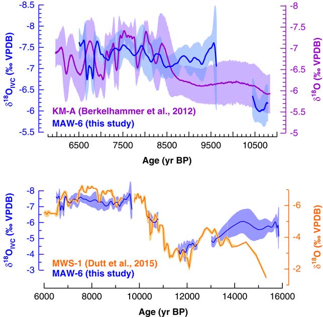
Comparison with other AM records
We chose three high-resolution and precisely dated records from Chinese caves (Dongge: Dykoski et al., Reference Dykoski, Edwards, Cheng, Yuan, Cai, Zhang, Lin, Qing, An and Revenaugh2005; Yamen: Yang et al., Reference Yang, Yuan, Cheng, Zhang, Qin, Lin, Zhu and Edwards2010; Kulishu: Ma et al., Reference Ma, Cheng, Tan, Edwards, Li, You, Duan, Wang and Kelly2012), the MWS-1 record from Mawmluh Cave, and the North Greenland Ice Core Project (NGRIP) ice core record from Greenland (Andersen et al., Reference Andersen, Azuma, Barnola, Bigler, Biscaye, Caillon and Chappellaz2004) to compare with our MAW-6 δ18OIVC record (Fig. 7). Comparison of the MAW-6 δ18OIVC record with these reconstructions reveals very similar centennial-millennial scale trends over the last deglaciation, further corroborating our interpretation of the record as a proxy for ISM strength (Fig. 7). However, more subtle differences are apparent as well. For example, whereas the other AM reconstructions indicate the weakest summer monsoons during the last glacial period (until ~14.5 ka), reflecting the pattern found in Greenland ice cores, MAW-6 records the weakest ISM conditions during the YD (Fig. 7). This is partly related to the adopted correction for ice volume and SST, which results in lighter δ18OIVC during the last glacial period, but the pattern is also apparent in the original δ18O record (Fig. 3). This is possibly a reflection of changes in regional seasonality in NE India, with a less vigorous ISM fed from proximal moisture sources, together with a wider spread of precipitation over the entire year during the YD. Testing this hypothesis requires seasonally resolved time series with highly robust chronologies.
(color online) Comparison of MAW-6 ice-volume-corrected δ18O (δ18OIVC) with δ18O records from the Indian summer monsoon (ISM) and broader Asian monsoon (AM) regions, as well as with the NGRIP ice core record. MAW-6 reflects and corroborates previous reconstructions from the AM region showing the weakest ISM after the deglaciation occurring during the Younger Dryas, and stronger ISM during the preceding Bølling-Allerød, as well as during the Holocene. VSMOW, Vienna standard mean ocean water; V-PDB, Vienna Pee Dee belemnite. NH, Northern Hemisphere; NHT, Northern Hemisphere Temperature.
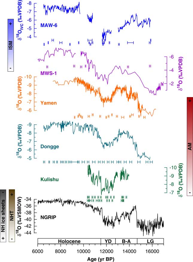
In addition, differences appear when comparing the B-A interstadial period in MAW-6 with other records. Whereas the AM records considered here all show a relatively rapid transition at the beginning and the end of the interval, with a plateau of lighter δ18O values during the B-A (attributed to increasing insolation; Ma et al., Reference Ma, Cheng, Tan, Edwards, Li, You, Duan, Wang and Kelly2012), MAW-6 shows a pattern of rapid isotopic depletion at ~14.5 ka followed by a gradual increase toward YD values that is more similar to the transition recorded in Greenland ice cores (Fig. 7). This might hint toward a close connection between NE India and the North Atlantic realm, driven by the westerlies. Evidence from paleoclimate records from central Asia suggests that the AM and westerly climates are tightly connected over glacial-interglacial cycles (Cheng et al., Reference Cheng, Spötl, Breitenbach, Sinha, Wassenburg, Jochum and Scholz2016b). Mawmluh Cave is located close to the Tibetan Plateau, with frequent influence of dry air masses from the Tibetan High during the winter season, and a closer connection to the westerly climate than found at the Chinese cave sites is thus plausible. However, this interpretation needs to be cautiously evaluated because of limited replication with the other δ18O record from Mawmluh Cave covering the B-A interval (MWS-1; Dutt et al., Reference Dutt, Gupta, Clemens, Cheng, Singh, Kathayat and Edwards2015), possibly related to chronological uncertainties in both records at this time.
The transition into the Holocene in MAW-6, although interrupted by a hiatus, shows substantially lighter δ18O values and thus ISM strengthening over time, similar to the record from Yamen Cave (Yang et al., Reference Yang, Yuan, Cheng, Zhang, Qin, Lin, Zhu and Edwards2010) and well-replicated in MWS-1. Conversely to the gradually lighter δ18O values found in the Yamen and Dongge cave records, however, both reconstructions from Mawmluh Cave show a short plateau of intermediate values between ~10.2 and 10.8 ka. In MAW-6, this interval is demarcated by two hiatuses; therefore, direct comparison with other records is difficult. This feature in the δ18O records could reflect slow retreat or even a short-lived advance of the Himalayan glaciers, related to the increase in moisture and precipitation (strengthening ISM) at the onset of the Holocene (Meyer et al., Reference Meyer, Hofmann, Gemmell, Haslinger, Häusler and Wangda2009). The glaciation in the mountain range and related cold air outflow from the Himalaya mountain range would have hampered the intrusion of the ISM somewhat longer in NE India. This explanation remains hypothetical however, especially because of the scarcity of data from the region.
Dynamic changes in the ISM
Dynamic regime changes in the ISM between the LG period and the EH were investigated using recurrence quantification analysis (Ozken et al., Reference Ozken, Eroglu, Stemler, Marwan, Bagci and Kurths2015; Eroglu et al., Reference Eroglu, McRobie, Ozken, Stemler, Wyrwoll, Breitenbach, Marwan and Kurths2016). We found a significant regime transition between LG and EH ISM, with more chaotic conditions during the LG, but higher predictability during the EH (Fig. 8). Disruption and weakening of the ISM during the LG, with frequent influence from westerly air masses and the Tibetan High, very likely result in less predictable conditions. This is similar to findings from complex network analysis of the AM, where weaker supraregional links were found during the cold/dry Little Ice Age (100–400 yr BP), suggesting that a weaker ISM is less predictable on a regional scale (Rehfeld et al., Reference Rehfeld, Marwan, Breitenbach and Kurths2012). During the EH, on the other hand, the strong seasonality induced by the ISM would lead to more regular annual cycles in precipitation and to a higher predictability.
Results of the TACTS analysis on MAW-6 δ18O. The cumulative probability distribution established through 5000 random realizations of recurrence determinism (DET) measure is shown by the blue line, with gray shading indicating the 95% confidence interval. The late glacial (LG) period and early Holocene (EH) are characterized by distinct DET measures (0.663 and 0.736, respectively). Although the LG is within the 95% confidence interval, the EH is outside, highlighting the high predictability of the Indian summer monsoon during this period. (For interpretation of the references to color in this figure legend, the reader is referred to the web version of this article.)
CONCLUSIONS
Stalagmite MAW-6 provides new paleoclimate data from Mawmluh Cave in NE India, covering the last deglaciation. We combine decadal-scale δ18O and δ13C measurements on MAW-6 to unravel climate change at regional and local scales over this period. A substantial postglacial shift toward more negative δ18O values is interpreted as strengthening of the ISM, with maximum expression during the EH. This pattern is in agreement with other reconstructions from Mawmluh Cave and the AM realm. Both the B-A and YD periods are clearly demarcated in the record as stronger and weaker ISM, respectively. δ13C is interpreted as reflecting local hydroclimatic conditions and is generally similar to δ18O, suggesting that a weak/strong ISM results in drier/wetter conditions at the study site. An intriguing exception to this rule is the YD, where combined δ18O and δ13C analysis suggests a reduction in precipitation seasonality, together with weakening of the ISM. Statistical time series analysis of the δ18O record reveals a significant regime transition over the last deglaciation, with less predictable ISM during the LG period and higher predictability during the Holocene, which we relate to the buildup of strong precipitation seasonality induced by the ISM.
ACKNOWLEDGMENTS
We gratefully acknowledge financial support from the Swiss National Fond (SNF Sinergia grant CRSI22 132646/1 and grant P2EZP2_172213), the German Science Foundation (DFG project MA4759/8-1—Impacts of uncertainties in climate data analysis [IUCliD]: approaches to working with measurements as a series of probability distributions—and grant no. RE3994-1/1), the National Natural Science Foundation of China (NSFC) grants 4123054 and 2013CB955902, the U.S. National Science Foundation grant 1103403, and the European Union’s Horizon 2020 Research and Innovation program under the Marie Skłodowska-Curie grant agreement no. 691037 (QUEST). We thank our Indian colleagues Bijay Mipun and Gregory Diengdoh for their logistic help. We thank Daniel Gebauer for support during fieldwork. We also thank Lydia Zehnder and Stewart Bishop (both at ETH Zürich) for assistance during XRD and stable isotope analysis, respectively. Tim Eglinton is acknowledged for financial support of F.A.L. We thank Ashish Sinha, Max Berkelhammer, James Baldini, Yanjun Cai, and two anonymous reviewers for constructive feedback and fruitful discussions on this and earlier versions of this manuscript. We thank the editors, Matthew Lachniet and Lewis Owen, for feedback and handling of the manuscript.
Supplementary Material
For supplementary material/s referred to in this article, please visit https://doi.org/10.1017/qua.2017.72


