


1. Introduction
Ocean surface waves exist at the interface of the water and air turbulent boundary layers and modulate exchanges of mass, momentum and energy across the atmosphere and the ocean (Melville Reference Melville1996; Deike Reference Deike2022). Ocean surface waves are characterized by a broad range of scales, growing under wind forcing, exchanging energy between wave modes through nonlinear interactions and dissipating energy due to wave breaking. Coupling with the underlying current modulates the kinematics of the surface waves.
An important application of wave–current interaction is the use of surface wave observations to infer underlying ocean currents. A well-established technique of this sort uses ground-based Doppler radar measurements, i.e. high-frequency radar systems, to measure the speed of ocean surface gravity waves to infer the ocean surface currents (Stewart & Joy Reference Stewart and Joy1974; Plant Reference Plant1990; Gommenginger et al. Reference Gommenginger, Srokosz, Challenor and Cotton2000; Lund et al. Reference Lund, Graber, Tamura, Collins III and Varlamov2015). Satellite-based Doppler radar instruments, like Doppler scatterometers and synthetic aperture radars, tend to operate at larger incidence angles and higher radar frequencies, and their radar returns come from shorter gravity–capillary waves. Unlike the gravity waves measured by high-frequency radar, gravity–capillary waves are more sensitive to the wind and to hydrodynamic and aerodynamic modulation associated with longer gravity waves (Stoffelen Reference Stoffelen1998; Chapron, Collard & Ardhuin Reference Chapron, Collard and Ardhuin2005; Johannessen et al. Reference Johannessen, Chapron, Collard, Kudryavtsev, Mouche, Akimov and Dagestad2008; Rodríguez et al. Reference Rodríguez, Wineteer, Perkovic-Martin, Gál, Stiles, Niamsuwan and Monje2018, Reference Rodríguez, Bourassa, Chelton, Farrar, Long, Perkovic-Martin and Samelson2019). However, interpreting Doppler measurements from spaceborne radars remains challenging because the kinematics of gravity–capillary waves in the presence of currents and multiscale wave coupling are not fully understood.
The sensitivity of spaceborne radars to small-scale gravity–capillary waves motivates a deeper understanding of the waves’ kinematics in the presence of an underlying current. The small-scale scatterers are composed of free and bound gravity–capillary waves (Plant, Dahl & Keller Reference Plant, Dahl and Keller1999), which are influenced by long-wave modulation and surface currents (Smith Reference Smith1986). These free and bound waves are nonlinearly coupled, complicating the interpretation of remote sensing data (Ardhuin et al. Reference Ardhuin, Chapron and Collard2009a ). Subsurface currents alter the observed frequency of surface waves, producing a Doppler shift carrying information about the underlying current, including the orbital velocity fields (Chapron et al. Reference Chapron, Collard and Ardhuin2005; Johannessen et al. Reference Johannessen, Chapron, Collard, Kudryavtsev, Mouche, Akimov and Dagestad2008). Currents modulate wave kinematics in a scale-dependent manner: shorter waves are Doppler-shifted by near-surface velocities, whereas longer waves are influenced by deeper currents (Stewart & Joy Reference Stewart and Joy1974). This physical effect has led to attempts to retrieve the water current profile with depth from remote sensing of the waves at multiple scales (Lund et al. Reference Lund, Graber, Tamura, Collins III and Varlamov2015; Smeltzer et al. Reference Smeltzer, Æsøy, Ådnøy and Ellingsen2019; Pizzo et al. Reference Pizzo, Lenain, Rømcke, Ellingsen and Smeltzer2023). Despite these advances, a predictive, dynamically consistent description of wave kinematics that incorporates nonlinear wave coupling and depth-varying currents remains incomplete.
Direct numerical simulations (DNS) solving for the air and water boundary layers and their coupling with gravity–capillary waves at the interface, spanning length scales from $O(10^{-3})$ $\mathrm{m}$
to
$\mathrm{m}$
to $O(10^{0})$ $\mathrm{m}$
, offer a promising framework to characterize wave kinematics in the presence of an evolving underwater turbulent current. Wu, Popinet & Deike (Reference Wu, Popinet and Deike2022) and Scapin et al. (Reference Scapin, Wu, Farrar, Chapron, Popinet and Deike2025, Reference Scapin, Wu, Farrar, Chapron, Popinet and Deike2026) demonstrated the ability of such DNS to reproduce realistic wave growth and underlying current and turbulence. Here, we extend this framework to simulate a broadband gravity–capillary wave spectrum forced by wind and interacting with a developing subsurface current. We characterize the time evolution of the space–time (frequency–wavenumber) spectrum and identify propagating wave modes along the linear dispersion relation and along bound harmonics. We show that waves exhibit a scale-dependent Doppler shift that is consistent with the theoretical framework of Stewart & Joy (Reference Stewart and Joy1974), where the Doppler shift velocity corresponds to the subsurface current in a surface-following reference frame. We further show that nonlinear wave–wave coupling generates multiple dispersion branches, and derive a nonlinear dispersion relation that incorporates both bound harmonics and depth-varying current effects. These results indicate that, under realistic ocean conditions with stronger scale separation and larger orbital velocities, Stokes drift will contribute significantly to the Doppler shift.
$\mathrm{m}$
, offer a promising framework to characterize wave kinematics in the presence of an evolving underwater turbulent current. Wu, Popinet & Deike (Reference Wu, Popinet and Deike2022) and Scapin et al. (Reference Scapin, Wu, Farrar, Chapron, Popinet and Deike2025, Reference Scapin, Wu, Farrar, Chapron, Popinet and Deike2026) demonstrated the ability of such DNS to reproduce realistic wave growth and underlying current and turbulence. Here, we extend this framework to simulate a broadband gravity–capillary wave spectrum forced by wind and interacting with a developing subsurface current. We characterize the time evolution of the space–time (frequency–wavenumber) spectrum and identify propagating wave modes along the linear dispersion relation and along bound harmonics. We show that waves exhibit a scale-dependent Doppler shift that is consistent with the theoretical framework of Stewart & Joy (Reference Stewart and Joy1974), where the Doppler shift velocity corresponds to the subsurface current in a surface-following reference frame. We further show that nonlinear wave–wave coupling generates multiple dispersion branches, and derive a nonlinear dispersion relation that incorporates both bound harmonics and depth-varying current effects. These results indicate that, under realistic ocean conditions with stronger scale separation and larger orbital velocities, Stokes drift will contribute significantly to the Doppler shift.
The paper is structured as follows: § 2 summarizes the theoretical background on wave kinematics with an underlying current; § 3 presents the DNS methodology. Section 4 characterizes the kinematics of waves under the evolving current, including Doppler shifts along the linear dispersion relation and the emergence of nonlinear dispersion branches. All results are then described in terms of a general nonlinear Doppler-shifted dispersion relation. Conclusions are given in § 5.
2. Theoretical background
2.1. Linear dispersion relation with an underlying current
The linear surface wave dispersion relation describes the propagation of free wave modes at the ocean surface. It links the wave angular frequency $\omega$
and wavenumber
$\omega$
and wavenumber $k$
, for gravity–capillary waves on the surface of deep water, and reads (Lamb Reference Lamb1932)
$k$
, for gravity–capillary waves on the surface of deep water, and reads (Lamb Reference Lamb1932) $\omega = \sqrt {gk +( {\sigma }/{\rho _w}) k^3}$
, where g is the acceleration due to gravity,
$\omega = \sqrt {gk +( {\sigma }/{\rho _w}) k^3}$
, where g is the acceleration due to gravity, $\sigma$
is the surface tension,
$\sigma$
is the surface tension, $\rho _w$
is the water density. The phase speed of the wave is then
$\rho _w$
is the water density. The phase speed of the wave is then $c=\omega /k$
. When surface waves are propagating on a vertically uniform current, the wave frequency is Doppler-shifted (Stewart & Joy Reference Stewart and Joy1974; Peregrine Reference Peregrine1976), obeying the Doppler-shifted linear dispersion relation
$c=\omega /k$
. When surface waves are propagating on a vertically uniform current, the wave frequency is Doppler-shifted (Stewart & Joy Reference Stewart and Joy1974; Peregrine Reference Peregrine1976), obeying the Doppler-shifted linear dispersion relation
 \begin{align} \omega (k) = \sqrt {gk + \frac {\sigma }{\rho _w} k^3} + \boldsymbol{u} \boldsymbol{\cdot }\boldsymbol{k}, \end{align}
where $\boldsymbol{u}$
is the current velocity vector and
$\boldsymbol{u}$
is the current velocity vector and $\boldsymbol{k}$
is the wavenumber vector. The observed frequency
$\boldsymbol{k}$
is the wavenumber vector. The observed frequency $\omega$
is shifted by the projection of the current velocity onto the wave propagation direction. For simplicity, we will assume alignment between waves and the current in the following discussion. Currents can vary significantly with depth, and the depth profile will modify their effect on wave dispersion. Stewart & Joy (Reference Stewart and Joy1974) demonstrated through linear theory that a depth-varying current induces a wavelength-dependent Doppler shift velocity. Each wave mode is affected by an effective current depending on its scale, with high-frequency modes (smaller wavelengths) affected by the current closer to the surface than lower-frequency modes (longer wavelengths). The Doppler-shifted linear dispersion relation under a depth-varying current is given by
$\omega$
is shifted by the projection of the current velocity onto the wave propagation direction. For simplicity, we will assume alignment between waves and the current in the following discussion. Currents can vary significantly with depth, and the depth profile will modify their effect on wave dispersion. Stewart & Joy (Reference Stewart and Joy1974) demonstrated through linear theory that a depth-varying current induces a wavelength-dependent Doppler shift velocity. Each wave mode is affected by an effective current depending on its scale, with high-frequency modes (smaller wavelengths) affected by the current closer to the surface than lower-frequency modes (longer wavelengths). The Doppler-shifted linear dispersion relation under a depth-varying current is given by
 \begin{align} \omega (k) = \sqrt {gk + \frac {\sigma }{\rho _w} k^3} + u_{\textit{eff}}(k) k, \end{align}
where $u_{\textit{eff}}(k)$
is the effective Doppler shift velocity for the mode
$u_{\textit{eff}}(k)$
is the effective Doppler shift velocity for the mode $k$
, given by (Stewart & Joy Reference Stewart and Joy1974)
$k$
, given by (Stewart & Joy Reference Stewart and Joy1974)
 \begin{align} u_{\textit{eff}}(k) = 2k \int _{0}^{\infty } u_L(z) e^{-2kz} {\rm d}z, \end{align}
where $z \ge 0$
denotes the depth measured downward from the mean water level, and
$z \ge 0$
denotes the depth measured downward from the mean water level, and $u_L(z)$
is the current responsible for the Doppler shift, given by the Lagrangian current (Stewart & Joy Reference Stewart and Joy1974; Ardhuin et al. Reference Ardhuin, Marié, Rascle, Forget and Roland2009b
; Pizzo et al. Reference Pizzo, Lenain, Rømcke, Ellingsen and Smeltzer2023). The Lagrangian current is the sum of the Stokes drift
$u_L(z)$
is the current responsible for the Doppler shift, given by the Lagrangian current (Stewart & Joy Reference Stewart and Joy1974; Ardhuin et al. Reference Ardhuin, Marié, Rascle, Forget and Roland2009b
; Pizzo et al. Reference Pizzo, Lenain, Rømcke, Ellingsen and Smeltzer2023). The Lagrangian current is the sum of the Stokes drift $u_{\textit{SD}}$
and the Eulerian current
$u_{\textit{SD}}$
and the Eulerian current $u_E$
,
$u_E$
, $u_L=u_{\textit{SD}}+u_{E}$
(Stewart & Joy Reference Stewart and Joy1974; Lund et al. Reference Lund, Graber, Tamura, Collins III and Varlamov2015; Pizzo et al. Reference Pizzo, Lenain, Rømcke, Ellingsen and Smeltzer2023). This framework has been used to infer the current at various depths from high-frequency radar measurements (Lund et al. Reference Lund, Graber, Tamura, Collins III and Varlamov2015; Pizzo et al. Reference Pizzo, Lenain, Rømcke, Ellingsen and Smeltzer2023; Smeltzer et al. Reference Smeltzer, Rømcke, Hearst and Ellingsen2023). Physically, the velocity signal of shorter waves decays more rapidly with depth, so these waves are only affected by the near-surface currents, while the longer waves penetrate more deeply and respond to currents extending farther into the water column. Because the wind-driven current and turbulence evolve in a coupled way,
$u_L=u_{\textit{SD}}+u_{E}$
(Stewart & Joy Reference Stewart and Joy1974; Lund et al. Reference Lund, Graber, Tamura, Collins III and Varlamov2015; Pizzo et al. Reference Pizzo, Lenain, Rømcke, Ellingsen and Smeltzer2023). This framework has been used to infer the current at various depths from high-frequency radar measurements (Lund et al. Reference Lund, Graber, Tamura, Collins III and Varlamov2015; Pizzo et al. Reference Pizzo, Lenain, Rømcke, Ellingsen and Smeltzer2023; Smeltzer et al. Reference Smeltzer, Rømcke, Hearst and Ellingsen2023). Physically, the velocity signal of shorter waves decays more rapidly with depth, so these waves are only affected by the near-surface currents, while the longer waves penetrate more deeply and respond to currents extending farther into the water column. Because the wind-driven current and turbulence evolve in a coupled way, $u_{\textit{eff}}(k)$
effectively includes both effects. The Stokes drift can be computed as (Kenyon Reference Kenyon1969; Pizzo, Melville & Deike Reference Pizzo, Melville and Deike2019)
$u_{\textit{eff}}(k)$
effectively includes both effects. The Stokes drift can be computed as (Kenyon Reference Kenyon1969; Pizzo, Melville & Deike Reference Pizzo, Melville and Deike2019)
 \begin{align} u_{\textit{SD}}(z) = 2g \int \frac {\phi (k) k ^2}{ \omega (k)} e^{-2kz} {\rm d}k, \end{align}
where $\phi (k) = \int k F(k,\theta ) {\rm d}\theta$
is the azimuthally integrated wave spectrum and
$\phi (k) = \int k F(k,\theta ) {\rm d}\theta$
is the azimuthally integrated wave spectrum and $F(k,\theta )$
is the directional wave spectrum, normalized such that
$F(k,\theta )$
is the directional wave spectrum, normalized such that $\overline {\eta ^2}=\int \phi (k){\rm d}k = \int \int F(k,\theta ) k {\rm d}k {\rm d}\theta$
. Note that, unless otherwise stated, integrations over the wavenumber are taken over
$\overline {\eta ^2}=\int \phi (k){\rm d}k = \int \int F(k,\theta ) k {\rm d}k {\rm d}\theta$
. Note that, unless otherwise stated, integrations over the wavenumber are taken over $k \in [0,\infty )$
, while integrations over the azimuthal angle are taken over
$k \in [0,\infty )$
, while integrations over the azimuthal angle are taken over $\theta \in [0,2\pi ]$
.
$\theta \in [0,2\pi ]$
.
In the gravity–capillary wave configuration studied here, the (developing) effective current will be evaluated from a wave-following frame of reference. Given the limited separation of scales between the longest gravity wave modes and the capillary waves, the Stokes drift will remain small compared with the surface following current.
2.2. Bound waves and the nonlinear dispersion relation
Small-amplitude surface waves are characterized by the linear dispersion relation. When the slope of a wave is high enough, bound harmonic modes will appear, exemplified by Stokes waves, or parasitic capillary waves (Longuet-Higgins Reference Longuet-Higgins1963b
; Fedorov & Melville Reference Fedorov and Melville1998; Fedorov, Melville & Rozenberg Reference Fedorov, Melville and Rozenberg1998; Herbert, Mordant & Falcon Reference Herbert, Mordant and Falcon2010). These bound harmonics correspond to shorter waves travelling at the speed of the longer carrier wave. The corresponding nonlinear dispersion relation can be understood in terms of resonant three-wave interaction (Phillips Reference Phillips1960), where weakly nonlinear wave modes interact and exchange energy, see Benjamin & Feir (Reference Benjamin and Feir1967), Zakharov (Reference Zakharov1968), Hasselmann & Hasselmann (Reference Hasselmann and Hasselmann1985) and Shavit et al. (Reference Shavit, Pusateri, Zhang, Pan, Maestrini, Onorato and Shatah2025). As a consequence, several nonlinear branches will appear as the wave slope increases. We use the term ‘nonlinear dispersion’ relation to describe bound waves, following the terminology from Herbert et al. (Reference Herbert, Mordant and Falcon2010); the term is also sometimes used differently in reference to finite amplitude effects where the wave propagation speed depends on the wave amplitude (e.g. for Stokes waves; see Lamb (Reference Lamb1932)), but that is not what is meant here. Considering a primary mode with wavenumber and angular frequency $(k^{*},\omega ^{*})$
, when its slope is high enough, nonlinear interaction with itself leads to higher frequency harmonics at (
$(k^{*},\omega ^{*})$
, when its slope is high enough, nonlinear interaction with itself leads to higher frequency harmonics at ( $2\omega ^*,2k^*$
), (
$2\omega ^*,2k^*$
), ( $3\omega ^*,3k^*$
), etc. (Phillips Reference Phillips1960). A bound harmonic wave mode of order
$3\omega ^*,3k^*$
), etc. (Phillips Reference Phillips1960). A bound harmonic wave mode of order $N$
, with its wavenumber
$N$
, with its wavenumber $k_N$
and frequency,
$k_N$
and frequency, $\omega _N$
is given by
$\omega _N$
is given by
 \begin{align} k_{N}= \textit{Nk}^{*} \hspace {1cm} \varOmega _{N} = N \omega ^{*}, \end{align}
with $N=2,3,\ldots$
the harmonic number (since
$N=2,3,\ldots$
the harmonic number (since $N=1$
is the primary mode). These components do not satisfy the linear dispersion relation as they are bound to the primary mode and will all travel at its speed,
$N=1$
is the primary mode). These components do not satisfy the linear dispersion relation as they are bound to the primary mode and will all travel at its speed, $c^{*} = \omega ^{*}/k^{*}$
. The nonlinear dispersion relation can then be derived (see also the discussion in Herbert et al. (Reference Herbert, Mordant and Falcon2010))
$c^{*} = \omega ^{*}/k^{*}$
. The nonlinear dispersion relation can then be derived (see also the discussion in Herbert et al. (Reference Herbert, Mordant and Falcon2010))
 \begin{align} \varOmega _{N} (k_{N}) = N \omega (k_N/N) = N \sqrt {gk_N/N + \frac {\sigma }{\rho _w} (k_N/N)^3}, \end{align}
where $\varOmega _{N}(k_N)$
is the angular frequency at
$\varOmega _{N}(k_N)$
is the angular frequency at $k$
in the
$k$
in the $N$
-branch, with
$N$
-branch, with $N=1,2,3 \ldots$
, and
$N=1,2,3 \ldots$
, and $\omega (k_N/N)$
is the frequency of the free mode of wavenumber
$\omega (k_N/N)$
is the frequency of the free mode of wavenumber $(k_N/N)$
to which they are bound. Thus, every
$(k_N/N)$
to which they are bound. Thus, every $k$
contained in the first main branch will have an associated
$k$
contained in the first main branch will have an associated $2k$
in the second branch (
$2k$
in the second branch ( $\varOmega _2(2k)$
), and an associated
$\varOmega _2(2k)$
), and an associated $3k$
in the third branch (
$3k$
in the third branch ( $\varOmega _3(3k)$
), and so on consecutively. In the presence of underwater currents, we can postulate the Doppler-shifted nonlinear dispersion relation
$\varOmega _3(3k)$
), and so on consecutively. In the presence of underwater currents, we can postulate the Doppler-shifted nonlinear dispersion relation
 \begin{align} \varOmega _{N} (k_{N}) = N \omega (k_N/N,t) = N \left [ \sqrt {gk_N/N + \frac {\sigma }{\rho _w} (k_N/N)^3} + u_{\textit{eff}}(k_N/N) k_N/N \right ]. \end{align}
These results apply to gravity and gravity–capillary waves and lead to nonlinear branches of propagation observed in laboratory experiments (Herbert et al. Reference Herbert, Mordant and Falcon2010; Falcon & Mordant Reference Falcon and Mordant2022), numerical simulations (Zhang & Pan Reference Zhang and Pan2022; Wu, Popinet & Deike Reference Wu, Popinet and Deike2023) and in ocean surface space–time analysis (from high-frequency radar (Lund et al. Reference Lund, Collins III, Graber, Terrill and Herbers2014, Reference Lund, Graber, Tamura, Collins III and Varlamov2015), stereo reconstruction (Peureux, Benetazzo & Ardhuin Reference Peureux, Benetazzo and Ardhuin2018) or polarimetric camera (Laxague & Zappa Reference Laxague and Zappa2020)).
2.3. Wave energy spectra in space and time
We consider the wave surface elevation $\eta (x,y,t)$
and will analyse the wave kinematics and dynamics using both the spatial wave spectrum and the space–time wave spectrum.
$\eta (x,y,t)$
and will analyse the wave kinematics and dynamics using both the spatial wave spectrum and the space–time wave spectrum.
The wave energy spectrum in space (at a given time $t$
) is obtained by performing a two-dimensional Fourier transform in space,
$t$
) is obtained by performing a two-dimensional Fourier transform in space,
 \begin{align} F(\boldsymbol{k},t)=\frac {1}{L_x L_y}\left |\int \int \eta (x,y,t) e^{-i(k_x x + k_y y)}{\rm d}x {\rm d}y \right |^2 , \end{align}
where $L_{x,y}$
is the length of the domain in
$L_{x,y}$
is the length of the domain in $x$
and
$x$
and $y$
. The spectrum originally computed in Cartesian coordinates can be expressed in polar coordinates
$y$
. The spectrum originally computed in Cartesian coordinates can be expressed in polar coordinates $F(k,\theta ,t)$
. The one-dimensional wave spectrum in space is then obtained by integration over all angles:
$F(k,\theta ,t)$
. The one-dimensional wave spectrum in space is then obtained by integration over all angles:
 \begin{align} \phi (k,t)=\int k F(k,\theta ,t){\rm d}\theta \mathrm{.} \end{align}
The wave energy spectrum in space and time is obtained by performing a two-dimensional Fourier transform in space and one-dimensional Fourier transform in time (over a specific interval),
 \begin{align} \varPhi (\boldsymbol{k},\omega )=\frac {1}{L_x L_y L_t}\left |\int \int \int \eta (x,y,t) e^{-i(k_x x + k_y y -\omega t)}{\rm d}x {\rm d}y {\rm d}t \right |^2 , \end{align}
where $L_t$
is the duration of the time interval
$L_t$
is the duration of the time interval $I$
. The spectrum can similarly be expressed in polar coordinates
$I$
. The spectrum can similarly be expressed in polar coordinates $\varPhi (k,\theta ,\omega )$
. The one-dimensional wave spectrum in space is then obtained by integration over all angles:
$\varPhi (k,\theta ,\omega )$
. The one-dimensional wave spectrum in space is then obtained by integration over all angles:
 \begin{align} \varPhi (k,\omega )=\int k \varPhi (k,\theta ,\omega ){\rm d}\theta \mathrm{.} \end{align}
In the following, we will primarily analyse the angle-integrated spatial spectrum $\phi (k,t)$
at various times, as well as the angle-integrated space–time spectrum
$\phi (k,t)$
at various times, as well as the angle-integrated space–time spectrum $\varPhi (k,\omega )$
over different time intervals
$\varPhi (k,\omega )$
over different time intervals $I$
.
$I$
.
3. Direct numerical simulations of gravity–capillary waves forced by wind and coupled to underwater current
To investigate the kinematics of ocean waves with wind and current effects, we perform DNS of a fully coupled three-dimensional air–water system over a broadbanded wave field, extending the work by Wu et al. (Reference Wu, Popinet and Deike2022) and Scapin et al. (Reference Scapin, Wu, Farrar, Chapron, Popinet and Deike2025, Reference Scapin, Wu, Farrar, Chapron, Popinet and Deike2026). We use the open-source solver Basilisk (Popinet Reference Popinet2009, Reference Popinet2015), solving the incompressible two-phase air–water Navier–Stokes equations employing a geometric volume-of-fluid method to accurately reconstruct the air–water interface (Popinet Reference Popinet2009), a momentum conserving scheme, and adaptive mesh refinement, see also Wu et al. (Reference Wu, Popinet and Deike2022) and Scapin et al. (Reference Scapin, Wu, Farrar, Chapron, Popinet and Deike2025, Reference Scapin, Wu, Farrar, Chapron, Popinet and Deike2026). Below, we review the governing equations and numerical methods employed (§ 3.1), describe the set-up and initialization of the simulations (§ 3.2) and illustrate the mean air and water flow along with the wave statistics (§ 3.3).
3.1. Governing equations and numerical methods
We solve the incompressible, two-phase Navier–Stokes equations with surface tension, which can be expressed in the one-fluid formulation as
 \begin{align} \partial _{t} \rho + \boldsymbol{\nabla }\boldsymbol{\cdot }(\rho \boldsymbol{u)} =0 , \\[-28pt] \nonumber \end{align}
 \begin{align} \rho (\partial _{t} \boldsymbol{u} + (\boldsymbol{u}\boldsymbol{\cdot }\boldsymbol{\nabla }) \boldsymbol{u}) = - \boldsymbol{\nabla }p + \rho \boldsymbol{g} + \boldsymbol{\nabla }\boldsymbol{\cdot }(\mu (\boldsymbol{\nabla }\boldsymbol{u} + \boldsymbol{\nabla }\boldsymbol{u}^{T})) + \sigma \varkappa \delta _{S} (\boldsymbol{x} -\boldsymbol{x_{\mathcal{F}}})\boldsymbol{n} , \\[-28pt] \nonumber \end{align}
 \begin{align} \boldsymbol{\nabla }\boldsymbol{\cdot }\boldsymbol{u} = 0 , \\[-12pt] \nonumber \end{align}
where $\boldsymbol{u}=(u,v,w)$
is the one-fluid velocity vector,
$\boldsymbol{u}=(u,v,w)$
is the one-fluid velocity vector, $\rho$
is the density,
$\rho$
is the density, $p$
is the pressure,
$p$
is the pressure, $\boldsymbol{g} = -g \boldsymbol{e_z}$
is the gravitational acceleration in
$\boldsymbol{g} = -g \boldsymbol{e_z}$
is the gravitational acceleration in $z$
direction,
$z$
direction, $\mu$
is the dynamic viscosity and
$\mu$
is the dynamic viscosity and $\sigma$
is the surface tension coefficient. The surface Dirac function
$\sigma$
is the surface tension coefficient. The surface Dirac function $\delta _{S} (\boldsymbol{x} -\boldsymbol{x_{\mathcal{F}}})$
is defined in a way that is only non-zero at the interface, located at
$\delta _{S} (\boldsymbol{x} -\boldsymbol{x_{\mathcal{F}}})$
is defined in a way that is only non-zero at the interface, located at $\boldsymbol{x_{\mathcal{F}}}$
. The vector
$\boldsymbol{x_{\mathcal{F}}}$
. The vector $\boldsymbol{n}$
is oriented pointing outward to the liquid domain, and
$\boldsymbol{n}$
is oriented pointing outward to the liquid domain, and $\varkappa =\boldsymbol{\nabla }\boldsymbol{\cdot }\boldsymbol{n}$
is the surface curvature. A scalar field representing the volume fraction of one of the two phases is introduced as
$\varkappa =\boldsymbol{\nabla }\boldsymbol{\cdot }\boldsymbol{n}$
is the surface curvature. A scalar field representing the volume fraction of one of the two phases is introduced as $\mathcal{F}(x,y,z,t)$
, which is set to 1 in the water phase and 0 in the air phase. Thus, for each phase, the physical properties (i.e. density and viscosity) are evaluated using an arithmetic average, based on the indicator function
$\mathcal{F}(x,y,z,t)$
, which is set to 1 in the water phase and 0 in the air phase. Thus, for each phase, the physical properties (i.e. density and viscosity) are evaluated using an arithmetic average, based on the indicator function $\mathcal{F}$
, of the corresponding properties of the water and air phases:
$\mathcal{F}$
, of the corresponding properties of the water and air phases:
 \begin{align} \rho = \mathcal{F}\rho _{w} + (1-\mathcal{F})\rho _{a} , \hspace {5mm} \mu = \mathcal{F}\mu _{w} + (1-\mathcal{F})\mu _{a}\mathrm{.} \end{align}
The governing two-phase Navier–Stokes (3.1), (3.2) and (3.3) are solved using an adaptive mesh refinement on an octree grid, implemented in Basilisk. The minimal cell size in the adaptive grid is $\Delta = L_0/2^{{L}}$
with
$\Delta = L_0/2^{{L}}$
with ${L}$
the maximum refinement level (Popinet Reference Popinet2015; Van Hooft et al. Reference Van Hooft, Popinet, van Heerwaarden, van der Linden, de Roode and van de Wiel2018; Mostert, Popinet & Deike Reference Mostert, Popinet and Deike2022). The grid is dynamically adapted in regions of interest with respect to the norm of the second derivative of the velocity and of the volume fraction, as in Wu et al. (Reference Wu, Popinet and Deike2022) and (Scapin et al. Reference Scapin, Wu, Farrar, Chapron, Popinet and Deike2025), reducing the overall computational cost to resolve a broader range of scales. An illustration of the adaptive grid is displayed in figure 1(b). The momentum equation is discretized employing a conservative scheme, with mass conservation achieved with an error typically below 0.01 % (Mostert et al. Reference Mostert, Popinet and Deike2022). The capillary and gravitational forces are discretized utilizing a well-balanced formulation (Popinet Reference Popinet2009), which preserves an exact equilibrium between the pressure gradient, capillary and gravitational forces under static conditions, minimizing the generation of artificial parasitic currents.
${L}$
the maximum refinement level (Popinet Reference Popinet2015; Van Hooft et al. Reference Van Hooft, Popinet, van Heerwaarden, van der Linden, de Roode and van de Wiel2018; Mostert, Popinet & Deike Reference Mostert, Popinet and Deike2022). The grid is dynamically adapted in regions of interest with respect to the norm of the second derivative of the velocity and of the volume fraction, as in Wu et al. (Reference Wu, Popinet and Deike2022) and (Scapin et al. Reference Scapin, Wu, Farrar, Chapron, Popinet and Deike2025), reducing the overall computational cost to resolve a broader range of scales. An illustration of the adaptive grid is displayed in figure 1(b). The momentum equation is discretized employing a conservative scheme, with mass conservation achieved with an error typically below 0.01 % (Mostert et al. Reference Mostert, Popinet and Deike2022). The capillary and gravitational forces are discretized utilizing a well-balanced formulation (Popinet Reference Popinet2009), which preserves an exact equilibrium between the pressure gradient, capillary and gravitational forces under static conditions, minimizing the generation of artificial parasitic currents.
3.2. Numerical set-up and initial conditions
The computational domain is a cubic box of side $L_0 = 4\lambda _p$
as displayed in figure 1, where
$L_0 = 4\lambda _p$
as displayed in figure 1, where $\lambda _p$
denotes the fundamental wavelength, and it comprises an air layer of height
$\lambda _p$
denotes the fundamental wavelength, and it comprises an air layer of height $h_a$
and a water layer of height
$h_a$
and a water layer of height $h_w$
. The resting water depth is
$h_w$
. The resting water depth is $h_w=L_0/(2\pi )=0.64\lambda _p$
, while the air domain height is
$h_w=L_0/(2\pi )=0.64\lambda _p$
, while the air domain height is $h_a=L_0(1-1/(2\pi ))=3.36\lambda _p$
. Periodic boundary conditions are applied in the two horizontal directions, i.e.
$h_a=L_0(1-1/(2\pi ))=3.36\lambda _p$
. Periodic boundary conditions are applied in the two horizontal directions, i.e. $x$
and
$x$
and $y$
, termed as the streamwise and spanwise directions, respectively, whereas free-slip boundary conditions are imposed at both the top and bottom boundaries (
$y$
, termed as the streamwise and spanwise directions, respectively, whereas free-slip boundary conditions are imposed at both the top and bottom boundaries ( $z=-h_w$
and
$z=-h_w$
and $z=h_a$
).
$z=h_a$
).
The wind-wave system can then be characterized by a set of non-dimensional parameters (Wu et al. Reference Wu, Popinet and Deike2022; Scapin et al. Reference Scapin, Wu, Farrar, Chapron, Popinet and Deike2025). We consider the air–water density ratio $\rho _w/\rho _a = 816$
, air and water height and depth are
$\rho _w/\rho _a = 816$
, air and water height and depth are $h_a/\lambda _p = 3.36$
and
$h_a/\lambda _p = 3.36$
and $h_w/\lambda _p = 0.64$
, which satisfies the deep-water waves condition, and allows for proper resolution of the air-side turbulent boundary layer. The remaining non-dimensional parameters are the ratio of wind friction velocity to wave phase speed,
$h_w/\lambda _p = 0.64$
, which satisfies the deep-water waves condition, and allows for proper resolution of the air-side turbulent boundary layer. The remaining non-dimensional parameters are the ratio of wind friction velocity to wave phase speed, $u_\ast /c$
, the friction Reynolds number,
$u_\ast /c$
, the friction Reynolds number, $ \textit{Re}_{\ast ,\lambda }=\rho _au_\ast \lambda _p/\mu _a$
, and the wave Reynolds number,
$ \textit{Re}_{\ast ,\lambda }=\rho _au_\ast \lambda _p/\mu _a$
, and the wave Reynolds number, $ \textit{Re}_w=\rho _w c\lambda _p/\mu _w$
, which quantifies the ratio of inertial to viscous forces in the air and in the water, and the Bond number,
$ \textit{Re}_w=\rho _w c\lambda _p/\mu _w$
, which quantifies the ratio of inertial to viscous forces in the air and in the water, and the Bond number, $Bo=(\rho _w-\rho _a)g/(k_p^2\sigma )$
, which compares gravity and surface tension forces and effectively sets the physical scale of the peak wavenumber (Deike et al. Reference Deike, Popinet and Melville2015, Reference Deike, Melville and Popinet2016; Mostert et al. Reference Mostert, Popinet and Deike2022). Finally, the initial wave slope characterizes the initial level of nonlinearities in the wave system,
$Bo=(\rho _w-\rho _a)g/(k_p^2\sigma )$
, which compares gravity and surface tension forces and effectively sets the physical scale of the peak wavenumber (Deike et al. Reference Deike, Popinet and Melville2015, Reference Deike, Melville and Popinet2016; Mostert et al. Reference Mostert, Popinet and Deike2022). Finally, the initial wave slope characterizes the initial level of nonlinearities in the wave system, $k_p H_s$
, where
$k_p H_s$
, where $H_s = 4 {\overline {\eta ^2}}$
is the significant wave height calculated from the mean square of the surface elevation
$H_s = 4 {\overline {\eta ^2}}$
is the significant wave height calculated from the mean square of the surface elevation $\eta$
and
$\eta$
and $k_p=2\pi /\lambda _p$
the peak wavenumber.
$k_p=2\pi /\lambda _p$
the peak wavenumber.
Here, we fix $ \textit{Re}_{\ast ,\lambda } = 214$
, ensuring that turbulence in the air develops within the inertial regime while keeping the computational cost manageable. The Bond number is set to
$ \textit{Re}_{\ast ,\lambda } = 214$
, ensuring that turbulence in the air develops within the inertial regime while keeping the computational cost manageable. The Bond number is set to $Bo = 200$
, enabling the study of gravity–capillary waves. The described kinematics remains valid across both capillary and gravity wave regimes, as demonstrated in Appendix B by considering cases with
$Bo = 200$
, enabling the study of gravity–capillary waves. The described kinematics remains valid across both capillary and gravity wave regimes, as demonstrated in Appendix B by considering cases with $Bo = 25$
and
$Bo = 25$
and $Bo = 1000$
. The Bond number sets the transition wavenumber
$Bo = 1000$
. The Bond number sets the transition wavenumber $k_c$
where gravity and surface tension are balanced (i.e.
$k_c$
where gravity and surface tension are balanced (i.e. $Bo(k_c)=1$
, so that
$Bo(k_c)=1$
, so that $k_c= k_p \sqrt {Bo}$
, and for example for
$k_c= k_p \sqrt {Bo}$
, and for example for $Bo=200$
,
$Bo=200$
, $k_c\approx 14k_p$
). We systematically vary the initial wave slope in the range
$k_c\approx 14k_p$
). We systematically vary the initial wave slope in the range $k_pH_s \in [0.04,0.16]$
and the wind forcing in the range
$k_pH_s \in [0.04,0.16]$
and the wind forcing in the range $u_\ast /c \in [0.25,0.75]$
. The wave Reynolds number is set to
$u_\ast /c \in [0.25,0.75]$
. The wave Reynolds number is set to $ \textit{Re}_w = 2.55 \boldsymbol{\times }10^4$
, high enough to limit viscous dissipation but low enough to be resolved with reasonable computational resources. As a result, the values of
$ \textit{Re}_w = 2.55 \boldsymbol{\times }10^4$
, high enough to limit viscous dissipation but low enough to be resolved with reasonable computational resources. As a result, the values of $u_\ast /c$
necessary for wave growth start at higher values than in field conditions where viscosity damping is much smaller, a trade-off discussed in Wu & Deike (Reference Wu and Deike2021), Wu et al. (Reference Wu, Popinet and Deike2022) and Scapin et al. (Reference Scapin, Wu, Farrar, Chapron, Popinet and Deike2025).
$u_\ast /c$
necessary for wave growth start at higher values than in field conditions where viscosity damping is much smaller, a trade-off discussed in Wu & Deike (Reference Wu and Deike2021), Wu et al. (Reference Wu, Popinet and Deike2022) and Scapin et al. (Reference Scapin, Wu, Farrar, Chapron, Popinet and Deike2025).
(a) Illustration of the computational set-up with a turbulent airflow (mean profile in light-blue line, while turbulent eddies are illustrated in black) $\eta \le z\le h_a$
, the wave field and the water field
$\eta \le z\le h_a$
, the wave field and the water field $-h_w\le z\le \eta$
). Here,
$-h_w\le z\le \eta$
). Here, $h_a$
and
$h_a$
and $h_w$
are the mean air and water mean heights. In the surface contour, dark-blue regions denote wave troughs, while the light blue regions indicate wave crests. The high resolution on the wave interface and associated boundary layer achieved thanks to the adaptive mesh refinement is illustrated in (b), with an example of the instantaneous streamwise velocity
$h_w$
are the mean air and water mean heights. In the surface contour, dark-blue regions denote wave troughs, while the light blue regions indicate wave crests. The high resolution on the wave interface and associated boundary layer achieved thanks to the adaptive mesh refinement is illustrated in (b), with an example of the instantaneous streamwise velocity $u$
on the midspanwise plane
$u$
on the midspanwise plane $y=0$
, normalized by
$y=0$
, normalized by $u_\ast$
in air and by
$u_\ast$
in air and by $c$
in water (b i) and zoomed view of the contour showing the adaptive numerical grid at
$c$
in water (b i) and zoomed view of the contour showing the adaptive numerical grid at ${L}=10$
in the near-wave region (b ii). Both contours refer to the physical time
${L}=10$
in the near-wave region (b ii). Both contours refer to the physical time $\omega t\approx 30$
for the case
$\omega t\approx 30$
for the case $u_\ast /c=0.5$
and
$u_\ast /c=0.5$
and $k_pH_s=0.16$
. Note that the aspect ratio is preserved in (a) and (b ii) and stretched in (b i) for visualization purposes.
$k_pH_s=0.16$
. Note that the aspect ratio is preserved in (a) and (b ii) and stretched in (b i) for visualization purposes.

To initialize the simulations, we extend the configuration described in Wu et al. (Reference Wu, Popinet and Deike2022) and Scapin et al. (Reference Scapin, Wu, Farrar, Chapron, Popinet and Deike2025) to a broadbanded wave field to investigate the response to wind forcing. Following the procedure presented in Wu et al. (Reference Wu, Popinet and Deike2022) and Scapin et al. (Reference Scapin, Wu, Farrar, Chapron, Popinet and Deike2025), the turbulent airflow consists of a fully developed turbulent boundary layer forced by a pressure gradient which sets the nominal friction velocity of the simulation $\tau _0 = \rho _a u_\ast ^{2} = h_a \partial _x p$
, where
$\tau _0 = \rho _a u_\ast ^{2} = h_a \partial _x p$
, where $u_\ast$
denotes the friction velocity and
$u_\ast$
denotes the friction velocity and $\partial _x p$
is the pressure gradient in the horizontal direction, and
$\partial _x p$
is the pressure gradient in the horizontal direction, and $\rho _a$
the air density. This pressure gradient forcing sustains continuous energy input, with waves gaining energy with time and transferring it to the water column. The turbulent boundary layer is generated up to a statistically steady state over a stationary broadbanded surface in a precursor simulation, see Wu et al. (Reference Wu, Popinet and Deike2022) and Scapin et al. (Reference Scapin, Wu, Farrar, Chapron, Popinet and Deike2025). Here, the initial directional wave spectrum follows a realistic wave spectrum (see Wu et al. (Reference Wu, Popinet and Deike2023)),
$\rho _a$
the air density. This pressure gradient forcing sustains continuous energy input, with waves gaining energy with time and transferring it to the water column. The turbulent boundary layer is generated up to a statistically steady state over a stationary broadbanded surface in a precursor simulation, see Wu et al. (Reference Wu, Popinet and Deike2022) and Scapin et al. (Reference Scapin, Wu, Farrar, Chapron, Popinet and Deike2025). Here, the initial directional wave spectrum follows a realistic wave spectrum (see Wu et al. (Reference Wu, Popinet and Deike2023)),
 \begin{align} F(k,\theta ) = \frac {\phi (k)}{k}\frac {\cos ^S(\theta )}{\int _{-\pi /2}^{\pi /2}\cos ^S(\theta ){\rm d}\theta } , \end{align}
where $S=5$
is the directional spreading parameter. We consider two spectral slope for the gravity and capillary regimes (Zakharov & Filonenko Reference Zakharov and Filonenko1966; Phillips Reference Phillips1985; Nazarenko Reference Nazarenko2011):
$S=5$
is the directional spreading parameter. We consider two spectral slope for the gravity and capillary regimes (Zakharov & Filonenko Reference Zakharov and Filonenko1966; Phillips Reference Phillips1985; Nazarenko Reference Nazarenko2011):
 \begin{align} \phi (k) = \begin{cases} Pk^{-3}\exp \left [-1.25\left (\dfrac {k_p}{k}\right )^2\right ]\quad &\text{if $k\lt k_c$} , \\ \mathcal{C}k^{-15/4}\quad &\text{if $k\ge k_c$}\mathrm{.} \end{cases} \end{align}
The parameter $P$
controls the initial energy level of the wave field, i.e. the initial wave slope
$P$
controls the initial energy level of the wave field, i.e. the initial wave slope $k_pH_s$
, and the constant
$k_pH_s$
, and the constant $\mathcal{C}$
is chosen to ensure continuity of
$\mathcal{C}$
is chosen to ensure continuity of $\phi (k)$
at the transition wavenumber
$\phi (k)$
at the transition wavenumber $k_c$
. From the initial wave spectrum, the initial wave elevation
$k_c$
. From the initial wave spectrum, the initial wave elevation $\eta (x,y,t=0)$
is obtained by a linear superposition of waves whose amplitudes correspond to the directional spectrum with random phases (Wu et al. Reference Wu, Popinet and Deike2023),
$\eta (x,y,t=0)$
is obtained by a linear superposition of waves whose amplitudes correspond to the directional spectrum with random phases (Wu et al. Reference Wu, Popinet and Deike2023),
 \begin{align} \eta (x,y) = \sum _{i=1}^{N_m}\sum _{j=1}^{N_m+1}a_{\textit{ij}}\cos (\psi _{\textit{ij}}) , \end{align}
with the amplitude $a_{\textit{ij}}= [2F(k_{xi},k_{yi})\Delta k_x\Delta k_y ]^{1/2}$
and the initial random phase
$a_{\textit{ij}}= [2F(k_{xi},k_{yi})\Delta k_x\Delta k_y ]^{1/2}$
and the initial random phase $\psi _{\textit{ij}}=k_{xi}x+k_{yi}y+\psi _{\textit{rand},\textit{ij}}$
. The wavenumber space is discretized with a uniform grid of
$\psi _{\textit{ij}}=k_{xi}x+k_{yi}y+\psi _{\textit{rand},\textit{ij}}$
. The wavenumber space is discretized with a uniform grid of $N_m\times N_m+1$
, and the wavenumbers are truncated and chosen at discrete values of
$N_m\times N_m+1$
, and the wavenumbers are truncated and chosen at discrete values of $k_x=ik_p/5$
for
$k_x=ik_p/5$
for $i\in [1,N_m]$
, and
$i\in [1,N_m]$
, and $k_y = jk_p/5$
for
$k_y = jk_p/5$
for $j\in [-N_m/2,N_m/2]$
, respectively, and here
$j\in [-N_m/2,N_m/2]$
, respectively, and here $N_m=64$
. The velocity in the water is initialized using the linear wave theory (Lamb Reference Lamb1932),
$N_m=64$
. The velocity in the water is initialized using the linear wave theory (Lamb Reference Lamb1932),
 \begin{align} \begin{cases} &u_w(x,y,z) = \displaystyle {\sum _{i=1}^{N_m}\sum _{j=1}^{N_m+1}\sqrt {gk_{\textit{ij}}}a_{\textit{ij}}\exp (k_{\textit{ij}}z)\cos (\psi _{\textit{ij}})\sin (\theta _{\textit{ij}})} , \\ &v_w(x,y,z) = \displaystyle {\sum _{i=1}^{N_m}\sum _{j=1}^{N_m+1}\sqrt {gk_{\textit{ij}}}a_{\textit{ij}}\exp (k_{\textit{ij}}z)\cos (\psi _{\textit{ij}})\sin (\theta _{\textit{ij}})} , \\ &w_w(x,y,z) = \displaystyle {\sum _{i=1}^{N_m}\sum _{j=1}^{N_m+1}\sqrt {gk_{\textit{ij}}}a_{\textit{ij}}\exp (k_{\textit{ij}}z)\sin (\psi _{\textit{ij}})} , \end{cases} \end{align}
where $k_{\textit{ij}}=\sqrt {k_{xi}^2+k_{yj}^2}$
and
$k_{\textit{ij}}=\sqrt {k_{xi}^2+k_{yj}^2}$
and $\theta _{\textit{ij}}=\tan ^{-1} (k_{yj}/k_{xi} )$
.
$\theta _{\textit{ij}}=\tan ^{-1} (k_{yj}/k_{xi} )$
.
The results presented throughout the paper use a refinement level ${L}=10$
, and results have been verified to be grid independent, as shown by a sensitivity study with
${L}=10$
, and results have been verified to be grid independent, as shown by a sensitivity study with ${L}=11$
shown in Appendix A. We also verify that the number of grid points is sufficient to resolve the viscous sublayer, the Kolmogorov length and the capillary length, as shown in Appendix A. When performing spectral analysis, we will focus on wave modes resolved with at least 25 cells per wavelength to ensure accurate resolution of the dispersion and energetics. Given the smallest cell size
${L}=11$
shown in Appendix A. We also verify that the number of grid points is sufficient to resolve the viscous sublayer, the Kolmogorov length and the capillary length, as shown in Appendix A. When performing spectral analysis, we will focus on wave modes resolved with at least 25 cells per wavelength to ensure accurate resolution of the dispersion and energetics. Given the smallest cell size $\Delta$
, the maximum resolved wavenumber we discuss in the paper is approximately
$\Delta$
, the maximum resolved wavenumber we discuss in the paper is approximately $k_{\textit{max}} \approx 10k_p$
.
$k_{\textit{max}} \approx 10k_p$
.
3.3. Illustration of the wind-wave dynamics and underwater current
We illustrate the coupled wind-wave-current system on a typical case, $k_pH_s=0.16$
,
$k_pH_s=0.16$
, $u_\ast /c_p=0.5$
,
$u_\ast /c_p=0.5$
, $Bo=200$
.
$Bo=200$
.
Illustration of the evolution of the surface elevation at different times: $t/T_p=0-14-34$
in (a), (b) and (c), together with the turbulent boundary layer in the air. (d) Time evolution of the potential wave energy, normalized by its initial value, showing an increase due to wind energy input. (e) Wave energy spectrum
$t/T_p=0-14-34$
in (a), (b) and (c), together with the turbulent boundary layer in the air. (d) Time evolution of the potential wave energy, normalized by its initial value, showing an increase due to wind energy input. (e) Wave energy spectrum $\phi (k)$
, normalized by its initial maximum value, plotted as a function of
$\phi (k)$
, normalized by its initial maximum value, plotted as a function of $k/k_p$
for increasing time
$k/k_p$
for increasing time $t/T_p$
(colour-coded). (f) Horizontally averaged air velocity profiles, for various times, demonstrating a statistically stationary turbulent boundary layer, which follows a rough wall log-law (see inset). (g) Water-side horizontally averaged velocity profiles (solid line) illustrating the transition from a viscous boundary layer to a turbulent regime. The Stokes drift is calculated and plotted in dotted lines. The inset in (g) shows the surface velocity for the mean profile (dots), averaged over intervals of four wave periods, evolving with time and following the similarity solution
$t/T_p$
(colour-coded). (f) Horizontally averaged air velocity profiles, for various times, demonstrating a statistically stationary turbulent boundary layer, which follows a rough wall log-law (see inset). (g) Water-side horizontally averaged velocity profiles (solid line) illustrating the transition from a viscous boundary layer to a turbulent regime. The Stokes drift is calculated and plotted in dotted lines. The inset in (g) shows the surface velocity for the mean profile (dots), averaged over intervals of four wave periods, evolving with time and following the similarity solution $u_s\propto \sqrt {t}$
(dashed black line, see Véron & Melville (Reference Véron and Melville2001); Wu & Deike (Reference Wu and Deike2021)), while the stars correspond to the Stokes drift value at the surface. For
$u_s\propto \sqrt {t}$
(dashed black line, see Véron & Melville (Reference Véron and Melville2001); Wu & Deike (Reference Wu and Deike2021)), while the stars correspond to the Stokes drift value at the surface. For $t/T_p \gt 20$
, the water transitions to turbulence, with the surface velocity reaching a steady value while the underwater shape transitions to a logarithmic profile. For the case
$t/T_p \gt 20$
, the water transitions to turbulence, with the surface velocity reaching a steady value while the underwater shape transitions to a logarithmic profile. For the case $k_pH_s=0.16$
,
$k_pH_s=0.16$
, $u_{*}/c=0.5$
and
$u_{*}/c=0.5$
and $Bo=200$
.
$Bo=200$
.

Typical snapshots of the wave surface and mean air velocity profiles are shown in figure 2, at $t/T_p = 0$
,
$t/T_p = 0$
, $14$
and
$14$
and $34$
in figure 2(a,b,c). The potential wave energy is shown in figure 2(d), and increases as a function of time due to the wind forcing. The overall growth (of the peak wave) can be quantitatively linked to the form drag and is grid converged (see Wu et al. Reference Wu, Popinet and Deike2022). In the present case
$34$
in figure 2(a,b,c). The potential wave energy is shown in figure 2(d), and increases as a function of time due to the wind forcing. The overall growth (of the peak wave) can be quantitatively linked to the form drag and is grid converged (see Wu et al. Reference Wu, Popinet and Deike2022). In the present case $k_p H_s$
increases from
$k_p H_s$
increases from $k_pH_s=0.16$
to
$k_pH_s=0.16$
to $k_pH_s=0.31$
over the nearly 40 peak wave periods
$k_pH_s=0.31$
over the nearly 40 peak wave periods $T_p$
that we simulated (time is colour-coded in all panels). Simulations are performed in a non-breaking regime (the wave amplitude never reaches breaking threshold). The time evolution of the spatial wave spectrum
$T_p$
that we simulated (time is colour-coded in all panels). Simulations are performed in a non-breaking regime (the wave amplitude never reaches breaking threshold). The time evolution of the spatial wave spectrum $\phi (k)$
is shown in figure 2(e), normalized by the maximum value of the spectra at the initial time
$\phi (k)$
is shown in figure 2(e), normalized by the maximum value of the spectra at the initial time $\phi _{0,\textit{max}}$
. The energy around the peak wavenumber exhibits sustained growth over time, while the high-wavenumber tail decays (due to viscous dissipation). The wavenumber separating growing and decaying modes corresponds to a balance between wind energy input (controlled by wave slope and wind forcing) and water-side viscous dissipation (controlled by the water Reynolds number), as discussed in Wu & Deike (Reference Wu and Deike2021). The horizontally averaged wind velocity profile obtained from the fully three-dimensional DNS is shown in figure 2(f), which corresponds to a turbulent boundary layer following the classic log-layer scaling
$\phi _{0,\textit{max}}$
. The energy around the peak wavenumber exhibits sustained growth over time, while the high-wavenumber tail decays (due to viscous dissipation). The wavenumber separating growing and decaying modes corresponds to a balance between wind energy input (controlled by wave slope and wind forcing) and water-side viscous dissipation (controlled by the water Reynolds number), as discussed in Wu & Deike (Reference Wu and Deike2021). The horizontally averaged wind velocity profile obtained from the fully three-dimensional DNS is shown in figure 2(f), which corresponds to a turbulent boundary layer following the classic log-layer scaling $\langle u\rangle (z)/u_* \approx 1/\kappa \log (z/z_0)$
, where
$\langle u\rangle (z)/u_* \approx 1/\kappa \log (z/z_0)$
, where $\kappa =0.41$
is the von Kármán constant and
$\kappa =0.41$
is the von Kármán constant and $z_0$
is a roughness length scale, fitted for this case,
$z_0$
is a roughness length scale, fitted for this case, $k_pz_0 \approx 3.2 \times 10^{-3}$
.
$k_pz_0 \approx 3.2 \times 10^{-3}$
.
Figure 2(g) shows the evolution of the current profile obtained in a wave-following coordinate system and averaged in the horizontal directions at each level. In this wind-driven current configuration, the initial mean water velocity is zero, and only the orbital velocity associated with the wave spectrum is set as an initial condition (Wu et al. Reference Wu, Popinet and Deike2022). A viscous boundary layer initially develops ( $t/T_p \lt 20$
) following the similarity solutions discussed by Véron & Melville (Reference Véron and Melville2001) and Wu & Deike (Reference Wu and Deike2021), with the surface velocity growing as
$t/T_p \lt 20$
) following the similarity solutions discussed by Véron & Melville (Reference Véron and Melville2001) and Wu & Deike (Reference Wu and Deike2021), with the surface velocity growing as $u_s \propto \sqrt {t/\nu _w}$
. The Stokes drift is calculated using (2.4) and plotted together with the mean current profile, and is significantly smaller than the mean current. At later times, the water current transitions to a turbulent state, with the near-surface velocity becoming roughly constant while the mean velocity profile undergoes a transition from an exponential shape to a logarithmic one. This change in the profile is responsible for the surface velocity reaching a steady value. We note that the use of wave-following coordinates to compute the current influences the horizontal velocity profile by preferentially sampling regions of higher positive and lower negative velocity – an effect analogous to the origin of Stokes drift (Pollard Reference Pollard1973). As a result, the velocity profile is not strictly Eulerian, but rather represents an Eulerian–Lagrangian combination.
$u_s \propto \sqrt {t/\nu _w}$
. The Stokes drift is calculated using (2.4) and plotted together with the mean current profile, and is significantly smaller than the mean current. At later times, the water current transitions to a turbulent state, with the near-surface velocity becoming roughly constant while the mean velocity profile undergoes a transition from an exponential shape to a logarithmic one. This change in the profile is responsible for the surface velocity reaching a steady value. We note that the use of wave-following coordinates to compute the current influences the horizontal velocity profile by preferentially sampling regions of higher positive and lower negative velocity – an effect analogous to the origin of Stokes drift (Pollard Reference Pollard1973). As a result, the velocity profile is not strictly Eulerian, but rather represents an Eulerian–Lagrangian combination.
4. Kinematics of gravity–capillary waves above an evolving current
We now discuss the space–time wave spectrum and quantify the kinematics of the waves. We identify wave energy propagation along the linear dispersion relation as well as the existence and development of nonlinear branches, both modes of propagation being Doppler-shifted.
4.1. Wave dispersion branches
We first consider the same case as in figure 2 to illustrate the existence of multiple branches of propagation. The wave energy space–time spectra $\varPhi (\omega ,k)$
are shown in figure 3 for increasing time windows
$\varPhi (\omega ,k)$
are shown in figure 3 for increasing time windows $I$
. Time windows are denoted as
$I$
. Time windows are denoted as $I$
and are chosen to be sufficiently long to resolve the peak (longest) wave and sufficiently short to capture a quasistationary response. For the extraction of spectral peaks, we tested windows of duration
$I$
and are chosen to be sufficiently long to resolve the peak (longest) wave and sufficiently short to capture a quasistationary response. For the extraction of spectral peaks, we tested windows of duration $5T_p$
to
$5T_p$
to $20T_p$
, which led to the same results for the peak location, while resolving the peak width shown in figure 3(b) require a window of at least
$20T_p$
, which led to the same results for the peak location, while resolving the peak width shown in figure 3(b) require a window of at least $9T_p$
. The total time analysis is also divided into two regimes: the first one when the underwater current is described by the viscous profile (figure 3
a,b,d,e) and the second regime when it has transitioned into a turbulent profile (figure 3
c,f).
$9T_p$
. The total time analysis is also divided into two regimes: the first one when the underwater current is described by the viscous profile (figure 3
a,b,d,e) and the second regime when it has transitioned into a turbulent profile (figure 3
c,f).
Wave kinematics revealed by the wave energy wavenumber-frequency spectrum $\varPhi (k,\omega )$
, for the case
$\varPhi (k,\omega )$
, for the case $k_pH_s=0.16$
,
$k_pH_s=0.16$
, $u_{*}/c=0.5$
and
$u_{*}/c=0.5$
and $Bo=200$
, for given time intervals
$Bo=200$
, for given time intervals $I$
(a,b,c) and corresponding cuts at fixed
$I$
(a,b,c) and corresponding cuts at fixed $k$
(d,e,f). Panels (a), (b), (d) and (e) show the earlier times (
$k$
(d,e,f). Panels (a), (b), (d) and (e) show the earlier times ( $t\le 20T_p$
), with the underwater current described by an accelerating viscous boundary layer. Distinct dispersion branches emerge, and deviations from the linear dispersion relation progressively increase (d,e) with three visible branches. Panels (c) and (f) show
$t\le 20T_p$
), with the underwater current described by an accelerating viscous boundary layer. Distinct dispersion branches emerge, and deviations from the linear dispersion relation progressively increase (d,e) with three visible branches. Panels (c) and (f) show $\varPhi (k,\omega )$
once the current has transitioned to turbulence. The solid white line is the linear dispersion relation,
$\varPhi (k,\omega )$
once the current has transitioned to turbulence. The solid white line is the linear dispersion relation, $\omega = \sqrt {gk + (\sigma /\rho _w) k^3}$
in (a), (b) and (c). Local spectral maxima are identified and marked: circles correspond to the
$\omega = \sqrt {gk + (\sigma /\rho _w) k^3}$
in (a), (b) and (c). Local spectral maxima are identified and marked: circles correspond to the $N=1$
branch (closest to the linear dispersion relation), squares to the
$N=1$
branch (closest to the linear dispersion relation), squares to the $N=2$
branch, and triangles to the
$N=2$
branch, and triangles to the $N=3$
branch. Vertical dashed lines indicate specific wavenumbers
$N=3$
branch. Vertical dashed lines indicate specific wavenumbers $k$
at which spectral cuts are shown in (b), (e) and (f).
$k$
at which spectral cuts are shown in (b), (e) and (f).

Figure 3(a) shows $\varPhi (k,\omega )$
for the earliest time window. The wave energy is located along different branches, with most of it along the linear dispersion relation for gravity–capillary waves, associated with free waves. White circles mark the global maxima in the
$\varPhi (k,\omega )$
for the earliest time window. The wave energy is located along different branches, with most of it along the linear dispersion relation for gravity–capillary waves, associated with free waves. White circles mark the global maxima in the $(k,\omega )$
space for each
$(k,\omega )$
space for each $k$
, corresponding to the primary (
$k$
, corresponding to the primary ( $N=1$
) branch. Additionally, wave energy is distributed along two other distinct branches, corresponding to bound harmonics. The local maxima associated with these secondary branches are indicated by red squares (
$N=1$
) branch. Additionally, wave energy is distributed along two other distinct branches, corresponding to bound harmonics. The local maxima associated with these secondary branches are indicated by red squares ( $N=2$
) and yellow triangles (
$N=2$
) and yellow triangles ( $N=3$
), at each
$N=3$
), at each $k$
. We observe that all branches are shifted due to the presence of the underlying current. Figure 3(d) shows spectral cuts at selected fixed wavenumbers
$k$
. We observe that all branches are shifted due to the presence of the underlying current. Figure 3(d) shows spectral cuts at selected fixed wavenumbers $k$
, illustrating these shifted branches. At
$k$
, illustrating these shifted branches. At $k/k_p=1$
, spectral energy remains concentrated on the shifted linear dispersion relation, whereas for higher wavenumbers, we distinctly observe multiple branches characterized by local maxima.
$k/k_p=1$
, spectral energy remains concentrated on the shifted linear dispersion relation, whereas for higher wavenumbers, we distinctly observe multiple branches characterized by local maxima.
Figures 3(b) and 3(c) present the same spectral analysis for later time windows. In figure 3(b), a stronger Doppler shift is visible due to an increased underlying current. Additionally, the energy at the peak of the main branch and at higher frequencies in the higher branches is more pronounced, as visible by comparing the amplitude of the bound modes (red squares and yellow triangles) between figures 3(d) and 3(b). Figure 3(d) reveals the appearance of a third dispersion branch, and a fourth branch, marked by orange circles, emerges at later times when the wave slope increases further.
Figure 3(c) corresponds to the regime with a turbulent underwater current. The surface velocity reaches a near-steady value, and the underwater velocity profile changes shape so that some wavenumbers are slightly slowed down. Comparing figure 3(f) with earlier cross-sections (figures 3
d and 3
e) confirms some of the trends already noted in figure 2(c). Most energy remains concentrated around the peak of the spectrum and increases over time. At higher wavenumbers (pink and green lines), the evolution appears to be branch-dependent. Modes within the primary gravity–capillary branch (white circles) exhibit a smaller relative energy increase at higher $k$
, and some even decrease, as seen by tracking the white circle at
$k$
, and some even decrease, as seen by tracking the white circle at $k = 4k_p$
(green line) across the different time intervals. At the same time, the
$k = 4k_p$
(green line) across the different time intervals. At the same time, the $N=2$
,
$N=2$
, $3$
branches (red squares and yellow triangles) show noticeable relative growth, indicating that the bound harmonics experience larger growth compared with the growth of the
$3$
branches (red squares and yellow triangles) show noticeable relative growth, indicating that the bound harmonics experience larger growth compared with the growth of the $N=1$
branch for a given value of
$N=1$
branch for a given value of $k$
. Each branch at a given
$k$
. Each branch at a given $k$
also broadens over time, with a stronger broadening for the bound harmonics
$k$
also broadens over time, with a stronger broadening for the bound harmonics $N=2,3$
than the main branch
$N=2,3$
than the main branch $N=1$
. The figures therefore show a simultaneous growth of the primary wave and its associated nonlinear bound harmonics, while the high-wavenumber free–wave components tend to decay. Finally, the number of visible branches increases with the overall steepness of the wave system.
$N=1$
. The figures therefore show a simultaneous growth of the primary wave and its associated nonlinear bound harmonics, while the high-wavenumber free–wave components tend to decay. Finally, the number of visible branches increases with the overall steepness of the wave system.
4.2. Quantifying the Doppler shift and the nonlinear dispersion relation
We now quantify the Doppler shift of the waves. We consider the maxima in ( $k-\omega$
) space, shown in figure 4. During the initial stages of propagation, when the current is described by the self-similar viscous boundary layer, the Doppler shifted dispersion relation is perfectly described by the Stewart & Joy (Reference Stewart and Joy1974) formula ((2.2) and (2.3)) using the current (shown in figure 1) extracted from the DNS (labelled
$k-\omega$
) space, shown in figure 4. During the initial stages of propagation, when the current is described by the self-similar viscous boundary layer, the Doppler shifted dispersion relation is perfectly described by the Stewart & Joy (Reference Stewart and Joy1974) formula ((2.2) and (2.3)) using the current (shown in figure 1) extracted from the DNS (labelled $u_{\textit{DNS}}$
in figure 4
a) for all time intervals. As mentioned above, the Stokes drift velocity is significantly smaller than the mean current evaluated in the wave-following frame (see inset figure 2
g). Once the water flow transitions to turbulence, the surface current velocity reaches a nearly constant value while the profile keeps evolving. The theoretical model given by (2.2) and (2.3) maintains a good accuracy with the turbulent water flow to characterize the Doppler shift magnitude, while a significant broadening of the wave spectrum is observed. We note that the transition from a viscous to a turbulent underwater current does not modify the validity of the Doppler-shifted nonlinear dispersion relation: the emergence of multiple branches is a nonlinear wave effect, while turbulence appears to modulate the spectral broadening. We illustrate the bound relationship between wave modes in the different branches in figure 4(c). A particular wavenumber
$u_{\textit{DNS}}$
in figure 4
a) for all time intervals. As mentioned above, the Stokes drift velocity is significantly smaller than the mean current evaluated in the wave-following frame (see inset figure 2
g). Once the water flow transitions to turbulence, the surface current velocity reaches a nearly constant value while the profile keeps evolving. The theoretical model given by (2.2) and (2.3) maintains a good accuracy with the turbulent water flow to characterize the Doppler shift magnitude, while a significant broadening of the wave spectrum is observed. We note that the transition from a viscous to a turbulent underwater current does not modify the validity of the Doppler-shifted nonlinear dispersion relation: the emergence of multiple branches is a nonlinear wave effect, while turbulence appears to modulate the spectral broadening. We illustrate the bound relationship between wave modes in the different branches in figure 4(c). A particular wavenumber $k_i^{*}$
in the first branch, with corresponding frequency
$k_i^{*}$
in the first branch, with corresponding frequency $\omega _i^{*}$
, travels with the same phase velocity as the harmonically related wavenumbers
$\omega _i^{*}$
, travels with the same phase velocity as the harmonically related wavenumbers $k_{2,i}=2k_i^{*}$
in the second branch and
$k_{2,i}=2k_i^{*}$
in the second branch and $k_{3,i}=3k_i^{*}$
in the third branch, depicted by the straight red line connecting these points. This visualization in figure 4(c) explicitly demonstrates how bound harmonics share the common phase velocity of the main/carrier wave described by resonant three-wave interaction in § 2.2.
$k_{3,i}=3k_i^{*}$
in the third branch, depicted by the straight red line connecting these points. This visualization in figure 4(c) explicitly demonstrates how bound harmonics share the common phase velocity of the main/carrier wave described by resonant three-wave interaction in § 2.2.
All times and harmonic branches are synthesized together in figure 4(d), applying the same procedure to the higher-order modes ( $N \gt 1$
). The bound harmonics are described by the Doppler-shifted nonlinear dispersion relation given by (2.7), significantly extending the applicability of the Stewart & Joy (Reference Stewart and Joy1974) framework to nonlinear bound modes.
$N \gt 1$
). The bound harmonics are described by the Doppler-shifted nonlinear dispersion relation given by (2.7), significantly extending the applicability of the Stewart & Joy (Reference Stewart and Joy1974) framework to nonlinear bound modes.
4.3. Reconstruction of the velocity profiles from the Doppler shift velocity
We discuss the effective velocity $u_{\textit{eff}}(k)$
(defined by (2.3)), which controls the Doppler shift of the dispersion relation in the Stewart & Joy (Reference Stewart and Joy1974) framework, and how the current profile can be reconstructed by inverse Laplace transform. We illustrate on the case discussed in figures 2, 3 and 4 (
$u_{\textit{eff}}(k)$
(defined by (2.3)), which controls the Doppler shift of the dispersion relation in the Stewart & Joy (Reference Stewart and Joy1974) framework, and how the current profile can be reconstructed by inverse Laplace transform. We illustrate on the case discussed in figures 2, 3 and 4 ( $k_pH_s=0.16$
,
$k_pH_s=0.16$
, $u_{*}/c =0.5$
and
$u_{*}/c =0.5$
and $Bo=200$
), and the results are similar for other tested parameters. The effective Doppler shift velocity is shown as a function of wavenumber
$Bo=200$
), and the results are similar for other tested parameters. The effective Doppler shift velocity is shown as a function of wavenumber $k$
in figure 5(a), for different time intervals, with the time colour-coded as in figure 2. During the viscous times, the effective velocity is increasing, while when the underwater current transitions to turbulence the effective velocity saturates for small wavenumber
$k$
in figure 5(a), for different time intervals, with the time colour-coded as in figure 2. During the viscous times, the effective velocity is increasing, while when the underwater current transitions to turbulence the effective velocity saturates for small wavenumber $k$
, and decays for bigger wavenumber
$k$
, and decays for bigger wavenumber $k$
. Since the actual angular velocity shifted is
$k$
. Since the actual angular velocity shifted is $u_{\textit{eff}} k$
the differences in times during the turbulence regime remain small. The velocity profile
$u_{\textit{eff}} k$
the differences in times during the turbulence regime remain small. The velocity profile $u_L(z)$
can be reconstructed from the effective velocity integral defined in (2.2), i.e.
$u_L(z)$
can be reconstructed from the effective velocity integral defined in (2.2), i.e. $u_{\textit{eff}}(k) = 2k\int _0^{\infty } u_L(z) e^{-2kz} \, {\rm d}z$
, which, introducing the variable
$u_{\textit{eff}}(k) = 2k\int _0^{\infty } u_L(z) e^{-2kz} \, {\rm d}z$
, which, introducing the variable $s = 2k$
, can be recognized as a Laplace transform:
$s = 2k$
, can be recognized as a Laplace transform:
 \begin{align} F(s) = \int _0^{\infty } u_L(z) e^{-s z} \, {\rm d}z = \frac {u_{\textit{eff}}(s/2)}{s}. \end{align}
Characterization of dispersion branches through the extraction of spectral local maxima for each $k$
at different time intervals I, for the case
$k$
at different time intervals I, for the case $k_pH_s=0.16$
,
$k_pH_s=0.16$
, $u_{*}/c=0.5$
and
$u_{*}/c=0.5$
and $Bo=200$
. (a) Maxima corresponding to the first (N = 1) branch (circles) during the early time (viscous boundary-layer), showing the temporal evolution of the Doppler shift. The solid black line represents the linear dispersion relation for gravity–capillary waves, while the solid coloured lines, each corresponding to a different time interval, include the Doppler shift as described by (2.7). (b) Same analysis as in (a), but now for intervals when the underwater flow has transitioned to turbulence. (c) Illustration of how each mode in higher harmonics branches (
$Bo=200$
. (a) Maxima corresponding to the first (N = 1) branch (circles) during the early time (viscous boundary-layer), showing the temporal evolution of the Doppler shift. The solid black line represents the linear dispersion relation for gravity–capillary waves, while the solid coloured lines, each corresponding to a different time interval, include the Doppler shift as described by (2.7). (b) Same analysis as in (a), but now for intervals when the underwater flow has transitioned to turbulence. (c) Illustration of how each mode in higher harmonics branches ( $N=2,3,4$
) travels at the same phase speed as a corresponding mode in the N = 1 branch. The red line indicates a constant wave phase speed shared by the higher-order bound harmonics. (d) Extends the procedure of (a) and (b), to include all times (viscous and turbulent regimes) and both the linear main branch (N = 1) and higher-order harmonic branches (
$N=2,3,4$
) travels at the same phase speed as a corresponding mode in the N = 1 branch. The red line indicates a constant wave phase speed shared by the higher-order bound harmonics. (d) Extends the procedure of (a) and (b), to include all times (viscous and turbulent regimes) and both the linear main branch (N = 1) and higher-order harmonic branches ( $N=2$
, squares; and
$N=2$
, squares; and $N=3$
, triangles). The dash–dotted and dotted lines represent the nonlinear dispersion relations for harmonics with
$N=3$
, triangles). The dash–dotted and dotted lines represent the nonlinear dispersion relations for harmonics with $N=2$
and
$N=2$
and $N=3$
, respectively, with the same colour coding for different times.
$N=3$
, respectively, with the same colour coding for different times.

(a) Effective velocity $u_{\textit{eff}}(k)$
as a function of the wavenumber
$u_{\textit{eff}}(k)$
as a function of the wavenumber $k$
for different time intervals (colour-coded). (b) The spatially and temporally averaged velocity profile beneath the water surface
$k$
for different time intervals (colour-coded). (b) The spatially and temporally averaged velocity profile beneath the water surface $\langle u_w\rangle _{\textit{DNS}}$
(solid lines) is compared with the reconstructed mean velocity profile
$\langle u_w\rangle _{\textit{DNS}}$
(solid lines) is compared with the reconstructed mean velocity profile $u_L^R$
(crosses) obtained from the effective velocity responsible for the Doppler shift in the frequency–wavenumber spectrum
$u_L^R$
(crosses) obtained from the effective velocity responsible for the Doppler shift in the frequency–wavenumber spectrum $\varPhi (k, \omega )$
. Each colour corresponds to a different time interval, with both profiles averaged over windows of four periods of the primary wave
$\varPhi (k, \omega )$
. Each colour corresponds to a different time interval, with both profiles averaged over windows of four periods of the primary wave $T_p$
. Both graphs presented for the case
$T_p$
. Both graphs presented for the case $k_pH_s=0.16$
,
$k_pH_s=0.16$
, $u_{*}/c=0.5$
and
$u_{*}/c=0.5$
and $Bo=200$
.
$Bo=200$
.

Thus, the original velocity profile is formally recovered by the inverse Laplace transform:
 \begin{align} u_L^R(z)= \mathcal{L}^{-1}\{F(s)\} = \mathcal{L}^{-1} \left \{\frac {u_{\textit{eff}}(s/2)}{s} \right \}. \end{align}
Because the Bromwich integral defining the inversion $\mathcal{L}^{-1}\{{\boldsymbol{\cdot }}\}$
is evaluated over a contour in the complex plane, while our effective velocity
$\mathcal{L}^{-1}\{{\boldsymbol{\cdot }}\}$
is evaluated over a contour in the complex plane, while our effective velocity $u_{\textit{eff}}$
is available only for real
$u_{\textit{eff}}$
is available only for real $s$
, we employ Schapery’s real-axis inversion method, which approximates the transform pair by a finite sum of real exponential functions, see e.g. Kuhlman (Reference Kuhlman2013) and Appendix C for details.
$s$
, we employ Schapery’s real-axis inversion method, which approximates the transform pair by a finite sum of real exponential functions, see e.g. Kuhlman (Reference Kuhlman2013) and Appendix C for details.
The values for the reconstructed velocity given by (4.2), are superposed and compared with the average water velocity from the DNS. Both the reconstructed profile and the measured mean velocity are normalized by the friction velocity $u_{*}$
for comparison. We observe a perfect agreement in the viscous regime, with a slight disagreement near the surface in the turbulent case, similar to the slight difference in the Doppler shift visible in figure 4. This analysis further confirms the applicability of the framework proposed in the Stewart & Joy (Reference Stewart and Joy1974) framework to understand the waves’ Doppler shift or reconstruct the mean velocity profile. Analysis of other cases yields similar agreement.
$u_{*}$
for comparison. We observe a perfect agreement in the viscous regime, with a slight disagreement near the surface in the turbulent case, similar to the slight difference in the Doppler shift visible in figure 4. This analysis further confirms the applicability of the framework proposed in the Stewart & Joy (Reference Stewart and Joy1974) framework to understand the waves’ Doppler shift or reconstruct the mean velocity profile. Analysis of other cases yields similar agreement.
4.4. Comparative analysis for a wide range of wind forcing and initial wave steepness
We now demonstrate the generality of the nonlinear dispersion relation under evolving currents, considering a broad range of wind forcing ( $u_*/c$
from
$u_*/c$
from $0.25$
to
$0.25$
to $0.5$
), initial steepness (
$0.5$
), initial steepness ( $k_p H_s$
from
$k_p H_s$
from $0.04$
to
$0.04$
to $0.16$
) and waves spanning gravity and capillary scales. Over time (the evolution of the simulations) the wave steepness can become as high as 0.32. Figure 6 summarizes results for all initial conditions and time evolution, including transition to turbulence (each configuration is simulated at least up to
$0.16$
) and waves spanning gravity and capillary scales. Over time (the evolution of the simulations) the wave steepness can become as high as 0.32. Figure 6 summarizes results for all initial conditions and time evolution, including transition to turbulence (each configuration is simulated at least up to $40t/T_p$
and typically up to
$40t/T_p$
and typically up to $60t/T_p$
). The time evolution of the underwater velocity profile is qualitatively similar across cases, but the transition to turbulence occurs at different times: increasing the wind stress (
$60t/T_p$
). The time evolution of the underwater velocity profile is qualitatively similar across cases, but the transition to turbulence occurs at different times: increasing the wind stress ( $u_*/c$
) leads to an earlier transition, and we also observe a sensitivity to
$u_*/c$
) leads to an earlier transition, and we also observe a sensitivity to $k_p H_s$
, with steeper waves triggering the transition sooner. Figure 6(a) further shows that the wave steepness controls the number of bound harmonic branches N.
$k_p H_s$
, with steeper waves triggering the transition sooner. Figure 6(a) further shows that the wave steepness controls the number of bound harmonic branches N.
Doppler shifted (nonlinear) dispersion relation. (a) The number of branches N as a function of the wave steepness $k_pH_s$
. (b,c) Maxima of the wave energy spectrum in the
$k_pH_s$
. (b,c) Maxima of the wave energy spectrum in the $(\omega ,k)$
space extracted at various times and for different initial conditions, indicated by distinct colour palettes, for the primary (
$(\omega ,k)$
space extracted at various times and for different initial conditions, indicated by distinct colour palettes, for the primary ( $N=1$
, circles) and bound harmonic (
$N=1$
, circles) and bound harmonic ( $N=2,3$
, squares and triangles, respectively) branches. The vertical axis in (b) shows the angular frequency
$N=2,3$
, squares and triangles, respectively) branches. The vertical axis in (b) shows the angular frequency $\varOmega _{N}/\omega _p$
as a function of the normalized wavenumber
$\varOmega _{N}/\omega _p$
as a function of the normalized wavenumber $Nk/k_p$
. The dashed line indicates the linear dispersion relation for gravity–capillary waves, whereas the dotted line corresponds to the linear dispersion relation for pure gravity waves. Panel (c) incorporates the Doppler shift
$Nk/k_p$
. The dashed line indicates the linear dispersion relation for gravity–capillary waves, whereas the dotted line corresponds to the linear dispersion relation for pure gravity waves. Panel (c) incorporates the Doppler shift $\varOmega _N-u_{\textit{eff}}k$
, so that data from the N = 1 harmonic collapse onto the linear gravity–capillary dispersion relation, while the bound harmonics (N = 2, 3) align with the gravity-wave dispersion relation, as they are bound to gravity wave carriers. Initial conditions include
$\varOmega _N-u_{\textit{eff}}k$
, so that data from the N = 1 harmonic collapse onto the linear gravity–capillary dispersion relation, while the bound harmonics (N = 2, 3) align with the gravity-wave dispersion relation, as they are bound to gravity wave carriers. Initial conditions include $k_pH_s$
ranging from
$k_pH_s$
ranging from $0.08$
to
$0.08$
to $0.16$
and wind forcing from
$0.16$
and wind forcing from $u_\ast /c =0.25,\,0.50$
. Lighter colour shades represent earlier times intervals
$u_\ast /c =0.25,\,0.50$
. Lighter colour shades represent earlier times intervals $I$
, while darker shades correspond to later times intervals
$I$
, while darker shades correspond to later times intervals $I$
. Each time interval used is at least
$I$
. Each time interval used is at least $9T_p$
.
$9T_p$
.

In figure 6(b,c), we consolidate all times, harmonic branches and initial conditions into a single representation, showing the nonlinear dispersion relation (2.6) and the Doppler-shifted nonlinear dispersion relation (2.7). By plotting $\varOmega _N$
as a function of
$\varOmega _N$
as a function of $Nk$
, we effectively fold the nonlinear harmonic branches onto their corresponding wave regime. Figure 6(b) highlights how different times exhibit distinct Doppler shifts due to the evolving current. Figure 6(c) incorporates the Doppler shift, showing
$Nk$
, we effectively fold the nonlinear harmonic branches onto their corresponding wave regime. Figure 6(b) highlights how different times exhibit distinct Doppler shifts due to the evolving current. Figure 6(c) incorporates the Doppler shift, showing $\varOmega _N-u_{\textit{eff}}k$
as a function of
$\varOmega _N-u_{\textit{eff}}k$
as a function of $Nk$
, and the temporal variations are accounted for, collapsing all data onto a single universal curve. We observe that the primary branch (
$Nk$
, and the temporal variations are accounted for, collapsing all data onto a single universal curve. We observe that the primary branch ( $N=1$
) closely follows the linear gravity–capillary dispersion relation. For higher harmonics (
$N=1$
) closely follows the linear gravity–capillary dispersion relation. For higher harmonics ( $N=2$
and
$N=2$
and $N=3$
), the bound harmonic branches collapse onto their corresponding free carrier modes, situated along the gravity-wave dispersion relation. All data collapse, demonstrating the general applicability of the nonlinear dispersion relation.
$N=3$
), the bound harmonic branches collapse onto their corresponding free carrier modes, situated along the gravity-wave dispersion relation. All data collapse, demonstrating the general applicability of the nonlinear dispersion relation.
The present $Bo=200$
configuration corresponds physically to a 1 m computational domain and a peak wavelength of approximately 25 cm. The primary free modes then propagate along the gravity–capillary dispersion relation at all considered frequencies, and bound harmonics are also within the gravity-wave regime. In the Appendix B we show that as the Bond number increases, the characteristic capillary-to-gravity-wave scale ratio shifts continuously towards gravity-dominated behaviour. When
$Bo=200$
configuration corresponds physically to a 1 m computational domain and a peak wavelength of approximately 25 cm. The primary free modes then propagate along the gravity–capillary dispersion relation at all considered frequencies, and bound harmonics are also within the gravity-wave regime. In the Appendix B we show that as the Bond number increases, the characteristic capillary-to-gravity-wave scale ratio shifts continuously towards gravity-dominated behaviour. When $Bo=1000$
, capillary effects become negligible, and all modes collapse onto the gravity-wave dispersion relation. Conversely, when
$Bo=1000$
, capillary effects become negligible, and all modes collapse onto the gravity-wave dispersion relation. Conversely, when $Bo=25$
, capillary wave effects dominate. These dynamics are all consistently captured by (2.7) and are illustrated in Appendix B.
$Bo=25$
, capillary wave effects dominate. These dynamics are all consistently captured by (2.7) and are illustrated in Appendix B.
4.5. Elevation statistics
We have discussed the development of nonlinear branches corresponding to bound harmonics, which are primarily related to the slope of the waves, here controlled mostly by the wind-induced growth, with an increase in the number of branches with the global slope of the waves $k_p H_s$
(figure 6). We now discuss the corresponding wave elevation statistics. Figure 7 shows the probability distribution function (PDF) of the normalized interface elevation
$k_p H_s$
(figure 6). We now discuss the corresponding wave elevation statistics. Figure 7 shows the probability distribution function (PDF) of the normalized interface elevation $z_{\eta }=\eta /\sigma _\eta$
, where
$z_{\eta }=\eta /\sigma _\eta$
, where $\sigma _\eta$
is the standard deviation of
$\sigma _\eta$
is the standard deviation of $\eta$
defined as
$\eta$
defined as $\sigma _\eta =\sqrt {\langle \eta ^2\rangle }$
. The distribution is close to Gaussian for cases with relatively low
$\sigma _\eta =\sqrt {\langle \eta ^2\rangle }$
. The distribution is close to Gaussian for cases with relatively low $k_p H_s$
as discussed in Longuet-Higgins (Reference Longuet-Higgins1952) (typically below 0.15, green and purple markers corresponding to weak forcing), i.e. described as
$k_p H_s$
as discussed in Longuet-Higgins (Reference Longuet-Higgins1952) (typically below 0.15, green and purple markers corresponding to weak forcing), i.e. described as $p(z_{\eta }) = 1/\sqrt {2 \pi } \exp (-z_{\eta }^2/2)$
. A nonlinear tail towards positive events develops for stronger wind forcing yielding skewed distributions. The skewness is quantified by the third standardized moment of the surface elevation as
$p(z_{\eta }) = 1/\sqrt {2 \pi } \exp (-z_{\eta }^2/2)$
. A nonlinear tail towards positive events develops for stronger wind forcing yielding skewed distributions. The skewness is quantified by the third standardized moment of the surface elevation as $\lambda _3= \langle (\eta /\sigma _\eta )^3\rangle$
, ranging from 0.11 to 0.24 in the stronger wind forcing cases. A vanishing skewness (
$\lambda _3= \langle (\eta /\sigma _\eta )^3\rangle$
, ranging from 0.11 to 0.24 in the stronger wind forcing cases. A vanishing skewness ( $\lambda _3 = 0$
) corresponds to a symmetric Gaussian distribution; positive skewness (
$\lambda _3 = 0$
) corresponds to a symmetric Gaussian distribution; positive skewness ( $\lambda _3 \gt 0$
) produces higher crests and shallower, more rounded troughs; while negative skewness (
$\lambda _3 \gt 0$
) produces higher crests and shallower, more rounded troughs; while negative skewness ( $\lambda _3 \lt 0$
) results in deeper troughs and lower crests (Longuet-Higgins Reference Longuet-Higgins1963a
; Fedele & Tayfun Reference Fedele and Tayfun2009). We also note that for relatively strong wind forcing, starting with the lowest wave slope, a nonlinear tail starts to develop even at low global wave slope, showing the importance of wind forcing and time of integration in the development of the wave field.
$\lambda _3 \lt 0$
) results in deeper troughs and lower crests (Longuet-Higgins Reference Longuet-Higgins1963a
; Fedele & Tayfun Reference Fedele and Tayfun2009). We also note that for relatively strong wind forcing, starting with the lowest wave slope, a nonlinear tail starts to develop even at low global wave slope, showing the importance of wind forcing and time of integration in the development of the wave field.
Following Fedele & Tayfun (Reference Fedele and Tayfun2009), skewed elevation statistics are expected to reflect the joint evolution of the surface wave mean steepness and spectral bandwidth. Skewed distribution can be compared with the Tayfun distribution (Tayfun Reference Tayfun1980), derived from weakly nonlinear potential theory for surface gravity waves accounting for second-order wave–wave interactions,
 \begin{align} P(z_{\eta }) = \frac {1 - \frac {7}{8}\mu _{nl}^2}{\sqrt {2\pi (1 + 3G + 2G^2)}} \exp \left (-\frac {G^2}{2\mu _{nl}^2}\right ), \end{align}
where $G = \sqrt {1 + 2\mu _{nl} z_{\eta }} - 1$
, and
$G = \sqrt {1 + 2\mu _{nl} z_{\eta }} - 1$
, and $\mu _{nl}$
is the nonlinear parameter, related to the skewness by
$\mu _{nl}$
is the nonlinear parameter, related to the skewness by $\mu _{nl} = \lambda _3/3$
, quantifying the effect of nonlinearity on the sea surface geometry. Positive values of
$\mu _{nl} = \lambda _3/3$
, quantifying the effect of nonlinearity on the sea surface geometry. Positive values of $\mu _{nl}$
produces positive skewness, and the distribution reduces to a Gaussian in the limit
$\mu _{nl}$
produces positive skewness, and the distribution reduces to a Gaussian in the limit $\mu _{nl} \rightarrow 0$
. As a second comparison, we consider the GC distribution (Longuet-Higgins Reference Longuet-Higgins1963a
), which introduces a perturbative correction to the Gaussian through a moment-based expansion, where the
$\mu _{nl} \rightarrow 0$
. As a second comparison, we consider the GC distribution (Longuet-Higgins Reference Longuet-Higgins1963a
), which introduces a perturbative correction to the Gaussian through a moment-based expansion, where the $\lambda _3$
term explicitly introduces asymmetry:
$\lambda _3$
term explicitly introduces asymmetry:
 \begin{align} p(z_{\eta }) = \frac {\exp \big(-z_{\eta }^2/2 \big)}{\sqrt {2\pi }} \left (1 + \frac {\lambda _3}{6} z_{\eta } \big(z_{\eta }^2 - 3 \big)\right ). \end{align}
(a) Probability density function of the normalized surface elevation $\eta /\sigma _\eta$
for different cases. Black solid line shows the normal Gaussian distribution. Colour dashed lines represent the Tayfun distribution for the three cases with high nonlinearities. For low wave slope, the elevation statistics is very close to the Gaussian one, while a nonlinear tail develops at higher wave slope. Inset: time evolution of the global wave steepness
$\eta /\sigma _\eta$
for different cases. Black solid line shows the normal Gaussian distribution. Colour dashed lines represent the Tayfun distribution for the three cases with high nonlinearities. For low wave slope, the elevation statistics is very close to the Gaussian one, while a nonlinear tail develops at higher wave slope. Inset: time evolution of the global wave steepness $k_pH_s$
for different initial wave slopes and wind forcing conditions. (b–d) Zoom of the right tail of the distribution for increasing initial wave steepness
$k_pH_s$
for different initial wave slopes and wind forcing conditions. (b–d) Zoom of the right tail of the distribution for increasing initial wave steepness $k_pHs =0.04, 0.08, 0.16$
and stronger wind forcing
$k_pHs =0.04, 0.08, 0.16$
and stronger wind forcing $u_*/c$
. Different linestyles denote the Gram–Charlier (GC) and Tayfun models, using the nonlinearity parameter
$u_*/c$
. Different linestyles denote the Gram–Charlier (GC) and Tayfun models, using the nonlinearity parameter $\mu = \lambda _3/3$
estimated directly from the DNS skewness.
$\mu = \lambda _3/3$
estimated directly from the DNS skewness.

Figure 7(b–d) compare both distributions with the DNS results for the strongest wind forcing case ( $u_*/c = 0.5$
). Both models capture the departure from Gaussian behaviour, which becomes more pronounced as the wave steepness
$u_*/c = 0.5$
). Both models capture the departure from Gaussian behaviour, which becomes more pronounced as the wave steepness $k_p H_s$
increases. The DNS-based estimate
$k_p H_s$
increases. The DNS-based estimate $\mu _{nl} = \lambda _3/3$
yields a good agreement with the data. The Tayfun distribution provides robust fit across all steepness values, while the GC expansion seems to underestimate tail probabilities at large
$\mu _{nl} = \lambda _3/3$
yields a good agreement with the data. The Tayfun distribution provides robust fit across all steepness values, while the GC expansion seems to underestimate tail probabilities at large $\eta /\sigma _\eta$
(Longuet-Higgins Reference Longuet-Higgins1963a
; Fedele & Tayfun Reference Fedele and Tayfun2009).
$\eta /\sigma _\eta$
(Longuet-Higgins Reference Longuet-Higgins1963a
; Fedele & Tayfun Reference Fedele and Tayfun2009).
The reported PDF are fairly similar to those reported from laboratory measurements for mechanically generated waves in Onorato et al. (Reference Onorato, Cavaleri, Fouques, Gramstad, Janssen, Monbaliu, Osborne, Pakozdi, Serio and Stansberg2009) and Michel et al. (Reference Michel, Bonnefoy, Ducrozet and Falcon2022).
5. Conclusions
We perform DNS of broadbanded gravity–capillary waves evolving under turbulent wind forcing, exploring a range of wind strengths and initial wave slopes within the non-breaking regime. The simulations resolve the coupled air–water dynamics and the development of the underwater current, from a viscous regime to a turbulent one. We characterize nonlinear waves, including bound harmonics forced by a turbulent boundary layer and under a viscous boundary layer or turbulent currents directly from DNS.
We show that nonlinear dispersion branches emerge as wave steepness increases, corresponding to bound harmonic modes propagating at the phase speed of their carrier waves. Furthermore, as the underwater flow transitions to turbulence, the kinematics of the waves remain well described by the Stewart & Joy (Reference Stewart and Joy1974) framework provided the actual current profile is employed. The number of nonlinear branches directly depends on the wave slope, and are observed for a range of wind conditions for gravity and gravity–capillary waves.
We introduce a nonlinear dispersion relation that describes these bound modes, based on three-wave interaction. We extend the classical framework proposed in Stewart & Joy (Reference Stewart and Joy1974) to these nonlinear bound harmonics and demonstrate that they follow the same depth-dependent Doppler shift as the carrier (free) modes. When this Doppler correction is evaluated using the current profile, all configurations and times collapse onto a single curve, demonstrating the generality of the formulation, again for both viscous and turbulent water-side currents. The underwater profile can be recovered from the Doppler shift by inverting the depth-dependent Doppler shift. A significant broadening of the wave energy spectrum at a given wavenumber is observed and might encode turbulence fluctuation information.
The framework developed here provides a basis for future investigations of regimes with stronger nonlinearities or incipient breaking could occur, energy transfer and detailed characterization of the spectral widening, as well as configuration with wider separation of scales where the Stokes drift from long wave will become important.
Acknowledgements
Computations were performed on the Stellar machine provided by the Cooperative Institute for Earth System Modeling (CIMES) and managed by Princeton Research Computing. N.S. acknowledges support from the High Meadows Environmental Institute Postdoctoral Teaching Program.
Funding
This work was supported by the National Science Foundation (grant 2318816 to L.D., Physical Oceanography program) and the NASA Ocean Vector Winds Science Team (grant 80NSSC23K0983 to L.D. and J.T.F.). C.M.B. acknowledges partial support from the New Jersey Economic Development Authority (NJEDA) Wind Institute Fellowship.
Declaration of interests
The authors report no conflict of interest.
Data availability statement
The open-source solver Basilisk used in this study is available at http://basilisk.fr/. The turbulent broadband wave set-up is mirrored on GitHub at https://github.com/DeikeLab/turbulent_setup/tree/broadbanded. The wind–current precursor case is available at https://github.com/DeikeLab/precursor. All postprocessing scripts are available at https://github.com/DeikeLab/post-processing-CMB.
Appendix A. Grid refinement study and numerical convergence
Two levels of grid refinement have been tested to verify numerical convergence and validate the results presented in the study. Throughout the paper, the simulations are carried out using a maximum refinement level of $L=10$
. To confirm the adequacy of this resolution, a more refined simulation at level
$L=10$
. To confirm the adequacy of this resolution, a more refined simulation at level $L=11$
has been performed for the main case discussed in the paper; with
$L=11$
has been performed for the main case discussed in the paper; with $k_pH_s=0.16 $
,
$k_pH_s=0.16 $
, $u_{*}/c =0.5$
and
$u_{*}/c =0.5$
and $Bo=200$
. Figure 8 illustrates the comparison between refinement levels
$Bo=200$
. Figure 8 illustrates the comparison between refinement levels $L=10$
and
$L=10$
and $L=11$
for several physical quantities.
$L=11$
for several physical quantities.
Sensitivity to grid resolution between $L=11$
and
$L=11$
and $L=10$
, for
$L=10$
, for $k_pH_s=0.16$
,
$k_pH_s=0.16$
, $u_{*}/c =0.5$
and
$u_{*}/c =0.5$
and $Bo=200$
. (a) Wave potential energy for
$Bo=200$
. (a) Wave potential energy for $L=11$
and
$L=11$
and $L=10$
as a function of time
$L=10$
as a function of time $t/T_p$
. Colour codes for the time are different for both resolutions and are used in the subsequent panels. (b) Spectrum for
$t/T_p$
. Colour codes for the time are different for both resolutions and are used in the subsequent panels. (b) Spectrum for $L=11$
(dashed line) and
$L=11$
(dashed line) and $L=10$
(solid line) at different times as a function of the normalized wavenumber
$L=10$
(solid line) at different times as a function of the normalized wavenumber $k/k_p$
. (c) Air-side mean velocity profile for
$k/k_p$
. (c) Air-side mean velocity profile for $L=11$
(dashed line) and
$L=11$
(dashed line) and $L=10$
(solid line) showing agreement in the inset for the scaling in both cases
$L=10$
(solid line) showing agreement in the inset for the scaling in both cases $\langle u \rangle / u_{*} \approx 1/\kappa \ln (z/ z_{0})$
. (d) Water-side mean velocity profiles for
$\langle u \rangle / u_{*} \approx 1/\kappa \ln (z/ z_{0})$
. (d) Water-side mean velocity profiles for $L=11$
(dashed line) and
$L=11$
(dashed line) and $L=10$
(solid line), the inset shows the agreement in the surface velocity values
$L=10$
(solid line), the inset shows the agreement in the surface velocity values $\langle u \rangle _{s}$
for both cases,
$\langle u \rangle _{s}$
for both cases, $L=11$
(stars) and
$L=11$
(stars) and $L=10$
(dots). A branches comparison has been done, for (e) the first harmonic
$L=10$
(dots). A branches comparison has been done, for (e) the first harmonic $N=1$
, (f) second harmonic
$N=1$
, (f) second harmonic $N=2$
and (d) third harmonic
$N=2$
and (d) third harmonic $N=3$
, showing good agreement for all of them at different levels of resolution.
$N=3$
, showing good agreement for all of them at different levels of resolution.

Figure 8(a) shows the time evolution of normalized potential wave energy $E(t)/E_0$
with almost no visible differences between both grid resolution, indicating convergence with the refinement level (stars L = 11, circles L = 10). The normalized wave energy spectra in figure 8(b),
$E(t)/E_0$
with almost no visible differences between both grid resolution, indicating convergence with the refinement level (stars L = 11, circles L = 10). The normalized wave energy spectra in figure 8(b), $\phi (k)/\phi _{0,{max}}$
, computed at various simulation times, demonstrate close agreement between the two refinement levels across all wavenumbers between
$\phi (k)/\phi _{0,{max}}$
, computed at various simulation times, demonstrate close agreement between the two refinement levels across all wavenumbers between $L=10$
and L = 11. Similarly, the mean velocity profiles in the air (figure 8
c) and water (figure 8
d) show excellent agreement between the two grid resolution. The inset in figure 8(c) further demonstrates the resolution of the logarithmic layer region for the air. The inset in figure 8(d) illustrates the time evolution of the normalized surface velocity, confirming minimal sensitivity to the grid refinement. In figure 8(e,f,g) we compare the branches extraction for both levels of refinement, which remain consistent in each case for the main harmonic figure 8(e), second figure 8(f) and third figure 8(g) harmonic. Overall, figure 8 demonstrates that all metrics presented in the main text are grid converged at
$L=10$
and L = 11. Similarly, the mean velocity profiles in the air (figure 8
c) and water (figure 8
d) show excellent agreement between the two grid resolution. The inset in figure 8(c) further demonstrates the resolution of the logarithmic layer region for the air. The inset in figure 8(d) illustrates the time evolution of the normalized surface velocity, confirming minimal sensitivity to the grid refinement. In figure 8(e,f,g) we compare the branches extraction for both levels of refinement, which remain consistent in each case for the main harmonic figure 8(e), second figure 8(f) and third figure 8(g) harmonic. Overall, figure 8 demonstrates that all metrics presented in the main text are grid converged at $L=10$
.
$L=10$
.
Table 1 provides the ratio of various characteristic lengths to the grid size, further confirming adequate resolution of the processes discussed in the paper; for the different configurations used in the main paper, as well as the gravity–capillary regimes discussed in Appendix B.
Comparison of the grid size with characteristic length scales for $L=10$
and
$L=10$
and $L=11$
. The columns indicate the simulations initial conditions (steepness
$L=11$
. The columns indicate the simulations initial conditions (steepness $k_pH_s$
, wind forcing
$k_pH_s$
, wind forcing $u_*/c$
, Bond number
$u_*/c$
, Bond number $Bo$
) and associated characteristic length scales compared with the grid size: root mean square of surface elevation
$Bo$
) and associated characteristic length scales compared with the grid size: root mean square of surface elevation $\sigma _{\eta }/\Delta$
, viscous length
$\sigma _{\eta }/\Delta$
, viscous length $\delta _{\nu }/\Delta$
and the Kolmogorov scale
$\delta _{\nu }/\Delta$
and the Kolmogorov scale $\eta _K/\Delta$
.
$\eta _K/\Delta$
.

The smallest grid size in the simulation is $\Delta = L_0/2^{L}$
, where
$\Delta = L_0/2^{L}$
, where $L_0$
is the domain length. As mentioned before, all simulations were performed with
$L_0$
is the domain length. As mentioned before, all simulations were performed with $L = 10$
with one sensitivity to the grid size using
$L = 10$
with one sensitivity to the grid size using $L=11$
. The root mean square surface elevation is calculated as
$L=11$
. The root mean square surface elevation is calculated as $\sigma _{\eta } = \sqrt {\langle \eta ^2 \rangle }$
. The ratio
$\sigma _{\eta } = \sqrt {\langle \eta ^2 \rangle }$
. The ratio $\sigma _{\eta }/\Delta \approx$
1.5–2 for a level of resolution
$\sigma _{\eta }/\Delta \approx$
1.5–2 for a level of resolution $L=10$
, and
$L=10$
, and $1.5-4$
for
$1.5-4$
for $L=11$
. The number of grid points per viscous length scale,
$L=11$
. The number of grid points per viscous length scale, $\delta _{\nu } = \lambda _p/\sqrt {Re}$
, is
$\delta _{\nu } = \lambda _p/\sqrt {Re}$
, is $\delta _{\nu }/\Delta \approx 1.6$
for
$\delta _{\nu }/\Delta \approx 1.6$
for $L=10$
(and approximately 3 for
$L=10$
(and approximately 3 for $L=11)$
. A turbulent-resolution criterion can be assessed by estimating the Kolmogorov length scale in the water phase using
$L=11)$
. A turbulent-resolution criterion can be assessed by estimating the Kolmogorov length scale in the water phase using $\eta _K = (\nu _w^{3}/\epsilon _{{max}})^{1/4}$
, where
$\eta _K = (\nu _w^{3}/\epsilon _{{max}})^{1/4}$
, where $\epsilon _{{max}}$
is the maximum dissipation rate
$\epsilon _{{max}}$
is the maximum dissipation rate $\varepsilon$
in the computational domain with
$\varepsilon$
in the computational domain with $\epsilon$
computed from the strain-rate tensor as
$\epsilon$
computed from the strain-rate tensor as $\epsilon = 2\nu _w S_{\textit{ij}}S_{\textit{ij}}$
, with
$\epsilon = 2\nu _w S_{\textit{ij}}S_{\textit{ij}}$
, with $S_{\textit{ij}} = ( {1}/{2}) (({\partial u_i}/{\partial x_j}) + ({\partial u_j}/{\partial x_i}) )$
. Across all configurations,
$S_{\textit{ij}} = ( {1}/{2}) (({\partial u_i}/{\partial x_j}) + ({\partial u_j}/{\partial x_i}) )$
. Across all configurations, $\eta _k/\Delta$
ranges from 2.1–2.6 at
$\eta _k/\Delta$
ranges from 2.1–2.6 at $L=10$
and 2.2–2.8 at
$L=10$
and 2.2–2.8 at $L=11$
. This confirms that the dissipative scales of the water-side turbulence are adequately resolved according to criteria discussed in (Pope Reference Pope2000).
$L=11$
. This confirms that the dissipative scales of the water-side turbulence are adequately resolved according to criteria discussed in (Pope Reference Pope2000).
Appendix B. Frequency–wavenumber wave spectrum at various Bond number
We perform the dispersion-relation analysis presented in the main text for $Bo=200$
, for cases at lower Bo number, which will centre more around capillary waves,
$Bo=200$
, for cases at lower Bo number, which will centre more around capillary waves, $Bo=25$
(figure 9) and higher Bond number, which will only imply gravity waves,
$Bo=25$
(figure 9) and higher Bond number, which will only imply gravity waves, $Bo=1000$
(figure 10). The case at
$Bo=1000$
(figure 10). The case at $Bo=1000$
is very similar to the one presented in the main text, with the main branch described by the Doppler-shifted dispersion relation, dominated by the gravity wave regime. As the wave amplitude increases, the nonlinear branches develop and broaden. The case at
$Bo=1000$
is very similar to the one presented in the main text, with the main branch described by the Doppler-shifted dispersion relation, dominated by the gravity wave regime. As the wave amplitude increases, the nonlinear branches develop and broaden. The case at $Bo=25$
follows a similar trend, with the nonlinear branches appearing very close to each other, a consequence of the functional form of the capillary wave dispersion relation.
$Bo=25$
follows a similar trend, with the nonlinear branches appearing very close to each other, a consequence of the functional form of the capillary wave dispersion relation.
Wave kinematics revealed by the wave energy wavenumber–frequency $\varPhi (k,\omega )$
for
$\varPhi (k,\omega )$
for $Bo=25$
for increasing time intervals
$Bo=25$
for increasing time intervals $I$
(a,b,c) and corresponding cuts at fixed k (d,e,f). Solid white line is the gravity–capillary dispersion relation,
$I$
(a,b,c) and corresponding cuts at fixed k (d,e,f). Solid white line is the gravity–capillary dispersion relation, $\omega = \sqrt {gk + (\sigma /\rho _w) k^3}$
, and the dashed white line is the capillary dispersion relation
$\omega = \sqrt {gk + (\sigma /\rho _w) k^3}$
, and the dashed white line is the capillary dispersion relation $\omega = \sqrt {(\sigma /\rho _w) k^3}$
. Local spectral maxima corresponding to different dispersion branches are identified and marked: circles represent the
$\omega = \sqrt {(\sigma /\rho _w) k^3}$
. Local spectral maxima corresponding to different dispersion branches are identified and marked: circles represent the $N=1$
branch (closest to the linear dispersion relation), squares
$N=1$
branch (closest to the linear dispersion relation), squares $N=2$
and triangles represent
$N=2$
and triangles represent $N=3$
. Vertical dashed lines indicate specific wavenumbers
$N=3$
. Vertical dashed lines indicate specific wavenumbers $k$
at which spectral cuts are shown in (d), (e) and (f).
$k$
at which spectral cuts are shown in (d), (e) and (f).

Wave kinematics revealed by the wave energy wavenumber–frequency $\varPhi (k,\omega )$
for
$\varPhi (k,\omega )$
for $Bo=1000$
for increasing time intervals
$Bo=1000$
for increasing time intervals $I$
(a,b,c) and corresponding cuts at fixed k (d,e,f). Solid white line is the gravity–capillary linear dispersion relation,
$I$
(a,b,c) and corresponding cuts at fixed k (d,e,f). Solid white line is the gravity–capillary linear dispersion relation, $\omega = \sqrt {gk + (\sigma /\rho _w) k^3}$
and dashed line is the gravity wave dispersion relation
$\omega = \sqrt {gk + (\sigma /\rho _w) k^3}$
and dashed line is the gravity wave dispersion relation $\omega =\sqrt {gk}$
. Local spectral maxima corresponding to different dispersion branches are identified and marked: circles represent the
$\omega =\sqrt {gk}$
. Local spectral maxima corresponding to different dispersion branches are identified and marked: circles represent the $N=1$
branch (closest to the linear dispersion relation), squares
$N=1$
branch (closest to the linear dispersion relation), squares $N=2$
and triangles represent
$N=2$
and triangles represent $N=3$
. Vertical dashed lines indicate specific wavenumbers
$N=3$
. Vertical dashed lines indicate specific wavenumbers $k$
at which spectral cuts are shown in (d), (e) and (f).
$k$
at which spectral cuts are shown in (d), (e) and (f).

The Doppler shifted different branches are plotted as a function of $Nk$
in the figure 11 (similar to figure 6 in the main text), figure 11(a) corresponds to
$Nk$
in the figure 11 (similar to figure 6 in the main text), figure 11(a) corresponds to $Bo=25$
and figure 11(b) corresponds to
$Bo=25$
and figure 11(b) corresponds to $Bo=1000$
. The case at high Bo number has all wave modes fold into the gravity wave dispersion relation. The case at
$Bo=1000$
. The case at high Bo number has all wave modes fold into the gravity wave dispersion relation. The case at $Bo=25$
has the
$Bo=25$
has the $N=1$
modes on the gravity–capillary dispersion relation (dominated by capillarity) while the
$N=1$
modes on the gravity–capillary dispersion relation (dominated by capillarity) while the $N=2$
and
$N=2$
and $N=3$
branches fold into the nonlinear capillary dispersion relation, which depends on the N value given the functional form of the nonlinear dispersion relation.
$N=3$
branches fold into the nonlinear capillary dispersion relation, which depends on the N value given the functional form of the nonlinear dispersion relation.
Different branches of the wave energy spectrum in the $(\omega ,k)$
space extracted at various times for same steepness
$(\omega ,k)$
space extracted at various times for same steepness $k_pH_s=0.16$
and velocity ratio
$k_pH_s=0.16$
and velocity ratio $u_*/c=0.5$
, for different Bond numbers. Panel (a) corresponds to
$u_*/c=0.5$
, for different Bond numbers. Panel (a) corresponds to $Bo=25$
, and (b) corresponds to
$Bo=25$
, and (b) corresponds to $Bo=1000$
.
$Bo=1000$
.

Appendix C. Details on the inverse Laplace transform to reconstruct the velocity profile
We present here details of how the inverse Laplace transform in (4.2) is computed.
Because the Bromwich integral defining $\mathcal{L}^{-1}$
is evaluated over a contour in the complex plane, while
$\mathcal{L}^{-1}$
is evaluated over a contour in the complex plane, while $u_{\textit{eff}}$
is available only for real
$u_{\textit{eff}}$
is available only for real $s=2k$
, we employ Schapery’s real–axis inversion formula (Kuhlman Reference Kuhlman2013), which approximates the transform pair by a finite sum of real exponentials:
$s=2k$
, we employ Schapery’s real–axis inversion formula (Kuhlman Reference Kuhlman2013), which approximates the transform pair by a finite sum of real exponentials:
 \begin{align} u_L^R(z) \approx f_s + \sum _{j=1}^{N_e} a_{\kern-1pt j} e^{-p_j z}. \end{align}
Here $f_s$
is the steady component (
$f_s$
is the steady component ( $u_L^R(z\to \infty )$
), estimated from the asymptotic value of the DNS velocity profile at the largest available depths. Here
$u_L^R(z\to \infty )$
), estimated from the asymptotic value of the DNS velocity profile at the largest available depths. Here $N_e$
is the number of exponentials,
$N_e$
is the number of exponentials, $p_j\gt 0$
are real-axis collocation points (often referred to as poles in Schapery’s method) and
$p_j\gt 0$
are real-axis collocation points (often referred to as poles in Schapery’s method) and $a_{\kern-1pt j}$
are the corresponding amplitudes to be determined. Taking the Laplace transform of (C1) yields
$a_{\kern-1pt j}$
are the corresponding amplitudes to be determined. Taking the Laplace transform of (C1) yields
 \begin{align} u_{\textit{eff}}(s)=\frac {f_s}{s}+\sum _{j=1}^{N_e}\frac {a_{\kern-1pt j}}{s+p_j}. \end{align}
Following Schapery’s real-axis inversion procedure, we enforce (C2) at the same set of poles $s=p_i$
, which leads to the linear system for the amplitudes
$s=p_i$
, which leads to the linear system for the amplitudes $a_{\kern-1pt j}$
:
$a_{\kern-1pt j}$
:
 \begin{align} \sum _{j=1}^{N_e}\frac {a_{\kern-1pt j}}{p_i+p_j} = u_{\textit{eff}}(p_i)-\frac {f_s}{p_i}, \qquad i=1,2,\ldots ,N_e. \end{align}
The right-hand side uses $u_{\textit{eff}}(p_i)$
obtained directly from the measured integral in (2.3) from the DNS, while
$u_{\textit{eff}}(p_i)$
obtained directly from the measured integral in (2.3) from the DNS, while $f_s/p_i$
removes the contribution of the steady term from each collocation equation.
$f_s/p_i$
removes the contribution of the steady term from each collocation equation.
To ensure numerical stability, the poles are chosen as a logarithmically spaced set, allowing to capture contributions from a wide range of vertical scales,
 \begin{align} p_j = p_{\textit{min}}\left (\frac {p_{\textit{max}}}{p_{\textit{min}}}\right )^{\tfrac {j-1}{N_e-1}}, \qquad j=1,\ldots ,N_e, \end{align}
where $p_{\textit{min}}$
and
$p_{\textit{min}}$
and $p_{\textit{max}}$
are proportional to the smallest and largest Laplace variables present in the data, scaled by an optimization factor
$p_{\textit{max}}$
are proportional to the smallest and largest Laplace variables present in the data, scaled by an optimization factor $\alpha$
. We explore a grid of
$\alpha$
. We explore a grid of $(N_e,\alpha )$
pairs and, for each choice, evaluate the reconstruction error
$(N_e,\alpha )$
pairs and, for each choice, evaluate the reconstruction error
 \begin{align}\textit{RMSE}=\sqrt {\frac {1}{n}\sum _{m=1}^{n} \bigl (u_{L}^R(z_m)-u_{{DNS}}(z_m)\bigr )^2} , \end{align}
where $u_{{DNS}}$
is the average velocity measured directly from DNS and
$u_{{DNS}}$
is the average velocity measured directly from DNS and $n$
is the number of spatial points. The optimal parameters were found at
$n$
is the number of spatial points. The optimal parameters were found at $N_e=3$
and a scale factor of
$N_e=3$
and a scale factor of $\alpha = 2.51$
, yielding an RMSE of
$\alpha = 2.51$
, yielding an RMSE of $0.12$
. These values are adopted throughout the present work to reconstruct the complete set of velocity profiles.
$0.12$
. These values are adopted throughout the present work to reconstruct the complete set of velocity profiles.


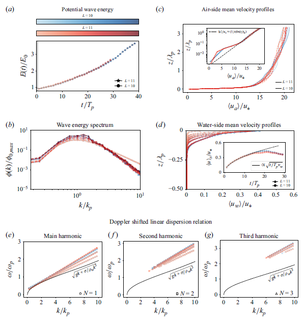


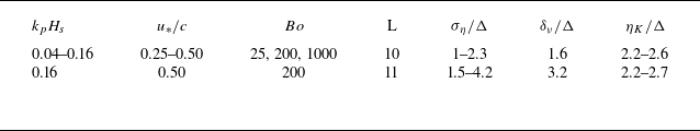


 Open access