


1. Introduction
Shannon [Reference Shannon29] presented a pivotal measure of information (uncertainty) called Shannon entropy, which has since become a foundational concept in various disciplines. Let  $X$ denote a nonnegative random variable characterized by probability density function (PDF) $f$ and cumulative distribution function (CDF) $F$. Then the mathematical representation of Shannon entropy for this variable is given by
 \begin{equation}
\mathcal{H}(X) = -\int_0^\infty f(x) \ln f(x) \, dx.
\end{equation}
\begin{equation}
\mathcal{H}(X) = -\int_0^\infty f(x) \ln f(x) \, dx.
\end{equation}Shannon entropy quantifies the anticipated quantity of information present in a dataset or message. A higher entropy value indicates greater uncertainty or unpredictability in the data. This measure has been extensively applied across a wide range of domains, including information theory, where it is used for coding and data compression, as well as in machine learning, statistical physics, and other areas requiring uncertainty quantification and data analysis. Its broad applicability has made it a fundamental tool in understanding information flow and complexity in various systems.
Lad et al. [Reference Lad, Sanfilippo and Agrò16] presented the notion of extropy, which is required to complement entropy, offering a dual perspective on the order and uncertainty of distributions. The article addresses long-standing inquiries regarding the axiomatization of information, thereby improving comprehension of probability measures. The introduction of extropy as a unique measure, its mathematical properties, and its applications in statistical scoring criteria, particularly in forecasting, are among the developments. For a random variable  $X$, its extropy is expressed as
 \begin{equation}
{J}(X) = -\frac{1}{2}\int_0^\infty f^2(x) dx.
\end{equation}
\begin{equation}
{J}(X) = -\frac{1}{2}\int_0^\infty f^2(x) dx.
\end{equation}For further recent developments on extropy, see [Reference Lad, Sanfilippo and Agrò17, Reference Qiu23–Reference Qiu, Wang and Wang25, Reference Yang, Xia and Hu36] and [Reference Noughabi and Jarrahiferiz22]. Since the density function required for extropy calculation is often unavailable in practical situations, [Reference Jahanshahi, Zarei and Khammar11] proposed the cumulative residual extropy (CREx), which relies on the survival function (SF) instead of the PDF. It is defined as
 \begin{equation}
\mathcal{J}(X) = -\frac{1}{2} \int_0^\infty \overline{F}^2(x) dx,
\end{equation}
\begin{equation}
\mathcal{J}(X) = -\frac{1}{2} \int_0^\infty \overline{F}^2(x) dx,
\end{equation}where  $\overline{F}$ denotes the SF of the random variable $X$.
$X$.
Subsequently, Nair and Sathar [Reference Nair and Sathar20] introduced the failure extropy (FEx), which depends on the CDF and is given by
 \begin{equation}
\mathcal{J}(X) = -\frac{1}{2} \int_A F^2(x)dx,
\end{equation}
\begin{equation}
\mathcal{J}(X) = -\frac{1}{2} \int_A F^2(x)dx,
\end{equation}where  $A$ denotes the support set of $X$. Kayal [Reference Kayal12] also studied DFEx and its weighted versions, and proposed nonparametric estimators based on the empirical distribution function.
However, both CREx and FEx are nonpositive, and FEx diverges for random variables with unbounded support. This limits its practical applicability and weakens its usefulness in risk and reliability analysis. This divergence motivates the need for a bounded and interpretable alternative. To overcome these drawbacks, Tahmasebi and Toomaz [Reference Tahmasebi and Toomaj33] proposed the negative cumulative extropy (NCEx), a finite and positive-valued measure suitable for risk and information analysis, defined as
 \begin{equation}
\mathcal{C}\mathcal{J}(X) = \frac{1}{2} \int_0^\infty \left(1 - F^2(x)\right) dx.
\end{equation}
\begin{equation}
\mathcal{C}\mathcal{J}(X) = \frac{1}{2} \int_0^\infty \left(1 - F^2(x)\right) dx.
\end{equation} Unlike FEx, the NCEx formulation remains finite even for unbounded distributions and offers a direct interpretation in terms of reliability characteristics. Tahmasebi and Toomaz [Reference Tahmasebi and Toomaj33] obtained several of its properties and demonstrated stronger connections with reliability quantities such as mean residual and mean past lifetimes compared to entropy or extropy-based analogues. They extended NCEx to the bivariate case for the random vector (RV)  $\mathbf X=(X_1, X_2)$, termed as bivariate NCEx (BNCEx), defined as
 \begin{equation}
\mathcal{C}\mathcal{J}(\mathbf X) = \frac{1}{2} \int_0^{\infty}\int_0^{\infty} (1 - F^2(x_1, x_2)) dx_2 dx_1.
\end{equation}
\begin{equation}
\mathcal{C}\mathcal{J}(\mathbf X) = \frac{1}{2} \int_0^{\infty}\int_0^{\infty} (1 - F^2(x_1, x_2)) dx_2 dx_1.
\end{equation} They also established its relationship with the Gini mean difference under independence. Almaspoor et al. {[Reference Almaspoor, Jafari and Tahmasebi2] studied the negative NCEx for concomitants of m-generalized order statistics within the Morgenstern family, and developed empirical estimators for NCEx. Noughabi [Reference Noughabi21] utilized NCEx for testing uniformity on  $[0,1]$, showing that NCEx lies between 0 and 1/2 for all densities on this interval and proposed a simple test statistic based on this property. Chakraborty et al. [Reference Chakraborty, Das and Pradhan4] introduced the weighted NCEx measure, which is related to reliability measures such as weighted mean residual and past lifetimes. They proposed a nonparametric estimator based on the empirical CDF and developed a consistent uniformity test that outperforms existing methods, particularly when alternatives have points near zero. For additional details on NCEx, see [Reference Chaudhary, Gupta and Sahu5, Reference Irshad, Maya, Archana and Tahmasebi10, Reference Tahmasebi, Ghimatgar and Ahmadzade32] and [Reference Shi, Sheng, Ahmadzade and Gao30].
In many practical situations, uncertainty may also relate to the past of a system. Consider a bivariate lifetime vector  $\mathbf{X}=(X_1,X_2)$ representing the lifetimes of two dependent components, systems, or organs. For fixed $t_1 \gt 0$ and $t_2 \gt 0$, suppose that both components have already failed before times $t_1$ and $t_2$, respectively; that is, the event $(X_1 \lt t_1,\; X_2 \lt t_2)$ has occurred. The bivariate past lifetime at $(t_1,t_2)$ is then defined as the conditional RV
  $
[(X_1,\, X_2)\;\big|\;(X_1 \lt t_1,\; X_2 \lt t_2)],
$ which describes the joint distribution of the two lifetimes given that failure in both components has already taken place before
$
[(X_1,\, X_2)\;\big|\;(X_1 \lt t_1,\; X_2 \lt t_2)],
$ which describes the joint distribution of the two lifetimes given that failure in both components has already taken place before  $(t_1,t_2)$. We denote this conditional vector by $\mathbf{X}^{\,\mathbf{t}} = [(X_1, X_2)\mid (X_1 \lt t_1,\; X_2 \lt t_2)],$ and refer to it as the bivariate past lifetime. The associated marginal past lifetimes are given by the conditional random variables
  $
\overline{X}_i = (X_i \mid X_1 \lt t_1,\; X_2 \lt t_2),~ i=1,2,$ which represent the individual component lifetimes restricted to the past region.
$
\overline{X}_i = (X_i \mid X_1 \lt t_1,\; X_2 \lt t_2),~ i=1,2,$ which represent the individual component lifetimes restricted to the past region.
The BNCEx defined in (1.6) is constructed for the RV  $\mathbf X$ and therefore does not properly capture the uncertainty associated with the conditional RV $\mathbf{X^t}$, which describes the joint past lifetimes. Since conditioning on $(X_1 \lt t_1,\,X_2 \lt t_2)$ alters the dependence structure and the distributional behavior of the components, the BNCEx measure becomes inadequate for assessing uncertainty in this transformed setting. Motivated by this limitation and by the substantial developments in past-lifetime analysis, see [Reference Ahmadi, Di Crescenzo and Longobardi1, Reference Ghosh and Kundu6, Reference Ghosh and Kundu7, Reference Kundu and Kundu14, Reference Kundu and Kundu15, Reference Raju, Sunoj and Rajesh26, Reference Sunoj and Linu31] and [Reference Viswakala, Gijo and Abdul Sathar34, Reference Viswakala, Thomas, Sathar and Gijo35], we extend the NCEx framework to the bivariate past lifetime setting. This allows us to develop a measure that accurately reflects the evolving uncertainty inherent in joint past lifetimes.
The subsequent sections of the paper are organized as follows: In Section 2, we study the bivariate dynamic NCEx and its behavior under monotonic transformations. Section 3 introduces a vector-valued definition of bivariate dynamic NCEx, explores the relationships of its components with various established reliability measures, and examines characterizations and stochastic orders. In Section 4, we develop an empirical estimator for the vector-valued bivariate dynamic NCEx, demonstrate its performance using simulated data, and apply it to two real data sets for further analysis. Finally, we summarize the findings and outline future works in Section 5.
2. Bivariate dynamic negative cumulative extropy
This section defines the NCEx for the bivariate RV  $\mathbf X^{\mathbf t}$, which is conditioned on the occurrence of both components falling below predetermined thresholds. The localized behavior of the joint distribution in the lower tail region can be captured by this conditional formulation, which is especially pertinent for applications in tail dependence analysis and risk assessment.
If  $\mathbf{X}=(X_1,X_2)$ denotes the lifetimes of two components in a system and both components have failed before times $t_1$ and $t_2$, respectively, then, provided that $F(t_1,t_2) \gt 0$, the uncertainty associated with the past lifetime of the system is quantified by the bivariate dynamic negative cumulative extropy (BDNCEx) of the conditional RV $(X_1,X_2)\mid (X_1 \lt t_1,\,X_2 \lt t_2)$, whose CDF is given by
  $
F(x_1,x_2;t_1,t_2)
= \frac{F(x_1,x_2)}{F(t_1,t_2)}.$ The BDNCEx is defined as
$
F(x_1,x_2;t_1,t_2)
= \frac{F(x_1,x_2)}{F(t_1,t_2)}.$ The BDNCEx is defined as
 \begin{equation}
\mathcal{C}\mathcal{J}^{\mathbf{X}}(t_1, t_2)
= \frac{1}{2} \int_{0}^{t_1} \int_{0}^{t_2}
\left( 1 - F^2(x_1,x_2;t_1,t_2) \right)
\, dx_2 \, dx_1.
\end{equation}
\begin{equation}
\mathcal{C}\mathcal{J}^{\mathbf{X}}(t_1, t_2)
= \frac{1}{2} \int_{0}^{t_1} \int_{0}^{t_2}
\left( 1 - F^2(x_1,x_2;t_1,t_2) \right)
\, dx_2 \, dx_1.
\end{equation} As  $t_1, t_2 \to \infty$, the conditioning becomes non-informative, and the measure in (2.7) reduces to the BNCEx defined in (1.6).
Now, we consider the following examples to illustrate the BDNCEx.
Example 2.1. Consider the bivariate generalized exponential (BGE) distribution with CDF
 \begin{align*}
F(x_1, x_2)
= \left(1 - e^{-\beta_1 x_1}\right)^{\theta}
+ \left(1 - e^{-\beta_2 x_2}\right)^{\theta}
- \left(1 - e^{-(\beta_1 x_1 + \beta_2 x_2)}\right)^{\theta},\quad
\beta_1, \beta_2 \gt 0, \theta \gt 0.
\end{align*}
\begin{align*}
F(x_1, x_2)
= \left(1 - e^{-\beta_1 x_1}\right)^{\theta}
+ \left(1 - e^{-\beta_2 x_2}\right)^{\theta}
- \left(1 - e^{-(\beta_1 x_1 + \beta_2 x_2)}\right)^{\theta},\quad
\beta_1, \beta_2 \gt 0, \theta \gt 0.
\end{align*} Using Eq. (2.7), we obtain the BDNCEx measure numerically for parameters  $\beta_1 = 1.5$, $\beta_2 = 1.2$, and $\theta = 0.8$, since deriving an explicit closed-form expression is analytically complex. The resulting plot is shown in Figure 1(a).
Example 2.2. Let  $\mathbf X$ be a nonnegative RV distributed as a bivariate generalized Rayleigh (BGR) distribution with CDF
 \begin{equation*}F(x_1, x_2)
= \left(1 - e^{-\tfrac{1}{2}\beta_1 x_1^2}\right)^{\theta}
+ \left(1 - e^{-\tfrac{1}{2}\beta_2 x_2^2}\right)^{\theta}
- \left(1 - e^{-\tfrac{1}{2}(\beta_1 x_1^2 + \beta_2 x_2^2)}\right)^{\theta},\quad
\beta_1, \beta_2 \gt 0, \theta \gt 0.
\end{equation*}
\begin{equation*}F(x_1, x_2)
= \left(1 - e^{-\tfrac{1}{2}\beta_1 x_1^2}\right)^{\theta}
+ \left(1 - e^{-\tfrac{1}{2}\beta_2 x_2^2}\right)^{\theta}
- \left(1 - e^{-\tfrac{1}{2}(\beta_1 x_1^2 + \beta_2 x_2^2)}\right)^{\theta},\quad
\beta_1, \beta_2 \gt 0, \theta \gt 0.
\end{equation*} Due to the analytical complexity involved in calculating BDNCEx, a closed-form solution is intractable. Therefore, we compute its values numerically for the parameter set  $\beta_1 = 1.8$, $\beta_2 = 2.2$, and $\theta = 0.9$. The resulting behavior is presented graphically in Figure 1(b). It is worth mentioning that, for the purpose of plotting the curves, the transformations $t_1 = -\ln x$ and $t_2 = -\ln y$ have been employed.
Plot of BDNCEx for BGE distribution (left) and BGR distribution (right).

In the following theorem, we investigate the behavior of BDNCEx under monotonic transformations.
Theorem 2.1 Assume that  $\mathbf X=(X_1,X_2)$ and $\mathbf{Y}=(Y_1,Y_2)$ be nonnegative bivariate RVs. Let $Y_i=\Phi_i (X_i)$, $i=1,2$, where $\Phi_i$ is a strictly monotone differentiable function. Then BDNCEx of $\mathbf Y=(Y_1,Y_2)$ is given by
 \begin{align*}
\mathcal{C}\mathcal{J}^{\mathbf Y}(t_1,t_2)= \begin{cases}&\frac{1}{2}\int_{\Phi_1^{-1}(0)}^{\Phi_1^{-1}(t_1)} \int_{\Phi_2^{-1}(0)}^{\Phi_2^{-1}(t_2)} \left(1-\left(\frac{F(x_1,x_2)}{F(\Phi_1^{-1}(t_1),\Phi_2^{-1}(t_2))}\right)^2\right)|J|\,dx_2\,dx_1,\\
&~~~\text{if}~\Phi_i~\text{is strictly increasing,}\\
&\frac{1}{2}\int_{\Phi_1^{-1}(t_1)}^{\Phi_1^{-1}(0)} \int_{\Phi_2^{-1}(t_2)}^{\Phi_2^{-1}(0)} \left(1-\left(\frac{\overline F(x_1,x_2)}{\overline F(\Phi_1^{-1}(t_1),\Phi_2^{-1}(t_2))}\right)^2\right)|J|\,dx_2\,dx_1,\\
&~~~\text{if}~\Phi_i~\text{is strictly decreasing,}
\end{cases}
\end{align*}
\begin{align*}
\mathcal{C}\mathcal{J}^{\mathbf Y}(t_1,t_2)= \begin{cases}&\frac{1}{2}\int_{\Phi_1^{-1}(0)}^{\Phi_1^{-1}(t_1)} \int_{\Phi_2^{-1}(0)}^{\Phi_2^{-1}(t_2)} \left(1-\left(\frac{F(x_1,x_2)}{F(\Phi_1^{-1}(t_1),\Phi_2^{-1}(t_2))}\right)^2\right)|J|\,dx_2\,dx_1,\\
&~~~\text{if}~\Phi_i~\text{is strictly increasing,}\\
&\frac{1}{2}\int_{\Phi_1^{-1}(t_1)}^{\Phi_1^{-1}(0)} \int_{\Phi_2^{-1}(t_2)}^{\Phi_2^{-1}(0)} \left(1-\left(\frac{\overline F(x_1,x_2)}{\overline F(\Phi_1^{-1}(t_1),\Phi_2^{-1}(t_2))}\right)^2\right)|J|\,dx_2\,dx_1,\\
&~~~\text{if}~\Phi_i~\text{is strictly decreasing,}
\end{cases}
\end{align*}where  $J=\frac{\partial }{\partial x_1}\Phi_1(x_1) \frac{\partial}{\partial x_2} \Phi(x_2)$ is the Jacobian transformation.
Proof. Let  $\mathbf{X}=(X_1,X_2)$ be a nonnegative bivariate RV with joint distribution function $F_{\mathbf X}(x_1,x_2)=P(X_1\le x_1,X_2\le x_2)$. Assume that $\Phi_i$ is strictly increasing. Then, for any $y_1,y_2 \gt 0$,
 \begin{align*}
F_{\mathbf Y}(y_1,y_2)
&=P(Y_1\le y_1,Y_2\le y_2)
=F_{\mathbf X}(\Phi_1^{-1}(y_1),\Phi_2^{-1}(y_2))
=F_{\mathbf X}(x_1,x_2).
\end{align*}
\begin{align*}
F_{\mathbf Y}(y_1,y_2)
&=P(Y_1\le y_1,Y_2\le y_2)
=F_{\mathbf X}(\Phi_1^{-1}(y_1),\Phi_2^{-1}(y_2))
=F_{\mathbf X}(x_1,x_2).
\end{align*}In particular,
 \begin{align*}
F_{\mathbf Y}(t_1,t_2)
=F_{\mathbf X}(\Phi_1^{-1}(t_1),\Phi_2^{-1}(t_2)).
\end{align*}
\begin{align*}
F_{\mathbf Y}(t_1,t_2)
=F_{\mathbf X}(\Phi_1^{-1}(t_1),\Phi_2^{-1}(t_2)).
\end{align*}Using the definition,
 \begin{equation}
\mathcal{C}\mathcal{J}^{\mathbf Y}(t_1,t_2)
=\frac{1}{2}\int_{0}^{t_1}\int_{0}^{t_2}
\left(1-F^2(y_1,y_2;t_1,t_2)\right)dy_2\,dy_1.
\end{equation}
\begin{equation}
\mathcal{C}\mathcal{J}^{\mathbf Y}(t_1,t_2)
=\frac{1}{2}\int_{0}^{t_1}\int_{0}^{t_2}
\left(1-F^2(y_1,y_2;t_1,t_2)\right)dy_2\,dy_1.
\end{equation} Utilizing the transformation  $x_i=\Phi_i^{-1}(y_i)$, we have
 \begin{equation*}
dy_2\,dy_1=\big|\Phi_1'(x_1)\Phi_2'(x_2)\big|\,dx_2\,dx_1=|J|\,dx_2\,dx_1,
\end{equation*}
\begin{equation*}
dy_2\,dy_1=\big|\Phi_1'(x_1)\Phi_2'(x_2)\big|\,dx_2\,dx_1=|J|\,dx_2\,dx_1,
\end{equation*}where  $J=\Phi_1'(x_1)\Phi_2'(x_2)$ is the Jacobian of transformation. Substituting into (2.8), we obtain
 \begin{equation*}
\mathcal{C}\mathcal{J}^{\mathbf Y}(t_1,t_2)
=\frac{1}{2}\int_{\Phi_1^{-1}(0)}^{\Phi_1^{-1}(t_1)}\int_{\Phi_2^{-1}(0)}^{\Phi_2^{-1}(t_2)}
\left(1-\left(\frac{F_{\mathbf X}(x_1,x_2)}{F_{\mathbf X}\left(\Phi_1^{-1}(t_1),\Phi_2^{-1}(t_2)\right)}\right)^2\right)
|J|\,dx_2\,dx_1.
\end{equation*}
\begin{equation*}
\mathcal{C}\mathcal{J}^{\mathbf Y}(t_1,t_2)
=\frac{1}{2}\int_{\Phi_1^{-1}(0)}^{\Phi_1^{-1}(t_1)}\int_{\Phi_2^{-1}(0)}^{\Phi_2^{-1}(t_2)}
\left(1-\left(\frac{F_{\mathbf X}(x_1,x_2)}{F_{\mathbf X}\left(\Phi_1^{-1}(t_1),\Phi_2^{-1}(t_2)\right)}\right)^2\right)
|J|\,dx_2\,dx_1.
\end{equation*} If  $\Phi_i$ is strictly decreasing, then $F_{\mathbf Y}(y_1,y_2)=\overline{F}_{\mathbf X}(x_1,x_2)$ and $F_{\mathbf Y}(t_1,t_2)=\overline{F}_{\mathbf X}(\Phi_1^{-1}(t_1),\Phi_2^{-1}(t_2))$. Therefore,
 \begin{equation*}
\mathcal{C}\mathcal{J}^{\mathbf Y}(t_1,t_2)
=\frac{1}{2}\int_{\Phi_1^{-1}(t_1)}^{\Phi_1^{-1}(0)}\int_{\Phi_2^{-1}(t_2)}^{\Phi_2^{-1}(0)}
\left(1-\left(\frac{\overline F_{\mathbf X}(x_1,x_2)}{\overline F_{\mathbf X}(\Phi_1^{-1}(t_1),\Phi_2^{-1}(t_2))}\right)^2\right)
|J|\,dx_2\,dx_1.
\end{equation*}
\begin{equation*}
\mathcal{C}\mathcal{J}^{\mathbf Y}(t_1,t_2)
=\frac{1}{2}\int_{\Phi_1^{-1}(t_1)}^{\Phi_1^{-1}(0)}\int_{\Phi_2^{-1}(t_2)}^{\Phi_2^{-1}(0)}
\left(1-\left(\frac{\overline F_{\mathbf X}(x_1,x_2)}{\overline F_{\mathbf X}(\Phi_1^{-1}(t_1),\Phi_2^{-1}(t_2))}\right)^2\right)
|J|\,dx_2\,dx_1.
\end{equation*}This completes the proof.
Next, we investigate BDNCEx under an affine transformation.
Theorem 2.2 Assume that  $\mathbf X=(X_1,X_2)$ and $\mathbf{Y}=(Y_1,Y_2)$ be nonnegative bivariate RVs. Let $Y_i=\beta_i+\theta_i X_i,~ \theta_i \gt 0 ~\text{and}~\beta_i\geq 0$ for $i=1,2$. Then
 \begin{align*}
\mathcal{C}\mathcal{J}^{\mathbf Y}(t_1,t_2)&=\theta_1\theta_2\,\mathcal{C}\mathcal{J}^{\mathbf{X}}\!\left(\frac{t_1-\beta_1}{\theta_1},\frac{t_2-\beta_2}{\theta_2}\right)
+\frac{t_1\beta_2 + t_2\beta_1 - \beta_1\beta_2}{2},~t_i\geq\beta_i.
\end{align*}
\begin{align*}
\mathcal{C}\mathcal{J}^{\mathbf Y}(t_1,t_2)&=\theta_1\theta_2\,\mathcal{C}\mathcal{J}^{\mathbf{X}}\!\left(\frac{t_1-\beta_1}{\theta_1},\frac{t_2-\beta_2}{\theta_2}\right)
+\frac{t_1\beta_2 + t_2\beta_1 - \beta_1\beta_2}{2},~t_i\geq\beta_i.
\end{align*}Proof. Let  $Y_i = \theta_i X_i + \beta_i,~~ \theta_i \gt 0,\ \beta_i\ge0,\ i=1,2.$ Then, for any $t_1,t_2$ satisfying $t_i\ge\beta_i$, the joint CDF of $\mathbf{Y}$ is given by
 \begin{equation*}
F_{\mathbf{Y}}(y_1,y_2)
= P\!\left(X_1\le \frac{y_1-\beta_1}{\theta_1},\, X_2\le \frac{y_2-\beta_2}{\theta_2}\right)
= F_{\mathbf{X}}\!\left(\frac{y_1-\beta_1}{\theta_1},\frac{y_2-\beta_2}{\theta_2}\right).
\end{equation*}
\begin{equation*}
F_{\mathbf{Y}}(y_1,y_2)
= P\!\left(X_1\le \frac{y_1-\beta_1}{\theta_1},\, X_2\le \frac{y_2-\beta_2}{\theta_2}\right)
= F_{\mathbf{X}}\!\left(\frac{y_1-\beta_1}{\theta_1},\frac{y_2-\beta_2}{\theta_2}\right).
\end{equation*} Define  $\tau_i = \frac{t_i-\beta_i}{\theta_i},~ i=1,2.$ Then, from (2.7), we have
 \begin{align*}
\mathcal{C}\mathcal{J}^{\mathbf{Y}}(t_1,t_2)
&= \frac{1}{2}\int_{0}^{t_1}\int_{0}^{t_2}
\left(1-F^2_{\mathbf Y}(y_1,y_2;t_1,t_2)\right)
dy_2\,dy_1\\[1ex]
&= \frac{1}{2}\int_{0}^{t_1}\int_{0}^{t_2}
\left(1-\left(\frac{F_{\mathbf{X}}\!\left(\frac{y_1-\beta_1}{\theta_1},\frac{y_2-\beta_2}{\theta_2}\right)}
{F_{\mathbf{X}}(\tau_1,\tau_2)}\right)^2\right)
dy_2\,dy_1.
\end{align*}
\begin{align*}
\mathcal{C}\mathcal{J}^{\mathbf{Y}}(t_1,t_2)
&= \frac{1}{2}\int_{0}^{t_1}\int_{0}^{t_2}
\left(1-F^2_{\mathbf Y}(y_1,y_2;t_1,t_2)\right)
dy_2\,dy_1\\[1ex]
&= \frac{1}{2}\int_{0}^{t_1}\int_{0}^{t_2}
\left(1-\left(\frac{F_{\mathbf{X}}\!\left(\frac{y_1-\beta_1}{\theta_1},\frac{y_2-\beta_2}{\theta_2}\right)}
{F_{\mathbf{X}}(\tau_1,\tau_2)}\right)^2\right)
dy_2\,dy_1.
\end{align*} Applying the change of variables  $y_1 = \theta_1 x_1 + \beta_1$ and $y_2 = \theta_2 x_2 + \beta_2,$ with corresponding Jacobian determinant $dy_1\,dy_2 = \theta_1\theta_2\,dx_1\,dx_2$, the limits of integration become $x_i \in \big[-\frac{\beta_i}{\theta_i},\,\tau_i\big]$. Hence,
 \begin{equation*}
\mathcal{C}\mathcal{J}^{\mathbf{Y}}(t_1,t_2)
= \frac{\theta_1\theta_2}{2}\int_{-\frac{\beta_1}{\theta_1}}^{\tau_1}\int_{-\frac{\beta_2}{\theta_2}}^{\tau_2}
\left(1-\left(\frac{F_{\mathbf{X}}(x_1,x_2)}{F_{\mathbf{X}}(\tau_1,\tau_2)}\right)^2\right)
dx_2\,dx_1.
\end{equation*}
\begin{equation*}
\mathcal{C}\mathcal{J}^{\mathbf{Y}}(t_1,t_2)
= \frac{\theta_1\theta_2}{2}\int_{-\frac{\beta_1}{\theta_1}}^{\tau_1}\int_{-\frac{\beta_2}{\theta_2}}^{\tau_2}
\left(1-\left(\frac{F_{\mathbf{X}}(x_1,x_2)}{F_{\mathbf{X}}(\tau_1,\tau_2)}\right)^2\right)
dx_2\,dx_1.
\end{equation*} Since  $\mathbf{X}$ is nonnegative, it follows that $F_{\mathbf{X}}(x_1,x_2)=0$ whenever $x_1 \lt 0$ or $x_2 \lt 0$. Therefore, we can decompose the above double integral over the rectangular domain $\big[-\frac{\beta_1}{\theta_1},\tau_1\big]\times\big[-\frac{\beta_2}{\theta_2},\tau_2\big]$ into subregions as follows:
 \begin{align*}
\mathcal{C}\mathcal{J}^{\mathbf{Y}}(t_1,t_2)
&= \frac{\theta_1\theta_2}{2}
\bigg[
\int_{0}^{\tau_1}\int_{0}^{\tau_2}
\left(1-\left(\frac{F_{\mathbf{X}}(x_1,x_2)}{F_{\mathbf{X}}(\tau_1,\tau_2)}\right)^2\right)
dx_2\,dx_1
+ \int_{0}^{\tau_1}\int_{-\frac{\beta_2}{\theta_2}}^{0} 1\,dx_2\,dx_1\\
&\quad
+ \int_{-\frac{\beta_1}{\theta_1}}^{0}\int_{0}^{\tau_2} 1\,dx_2\,dx_1
+ \int_{-\frac{\beta_1}{\theta_1}}^{0}\int_{-\frac{\beta_2}{\theta_2}}^{0} 1\,dx_2\,dx_1
\bigg].
\end{align*}
\begin{align*}
\mathcal{C}\mathcal{J}^{\mathbf{Y}}(t_1,t_2)
&= \frac{\theta_1\theta_2}{2}
\bigg[
\int_{0}^{\tau_1}\int_{0}^{\tau_2}
\left(1-\left(\frac{F_{\mathbf{X}}(x_1,x_2)}{F_{\mathbf{X}}(\tau_1,\tau_2)}\right)^2\right)
dx_2\,dx_1
+ \int_{0}^{\tau_1}\int_{-\frac{\beta_2}{\theta_2}}^{0} 1\,dx_2\,dx_1\\
&\quad
+ \int_{-\frac{\beta_1}{\theta_1}}^{0}\int_{0}^{\tau_2} 1\,dx_2\,dx_1
+ \int_{-\frac{\beta_1}{\theta_1}}^{0}\int_{-\frac{\beta_2}{\theta_2}}^{0} 1\,dx_2\,dx_1
\bigg].
\end{align*}Evaluating each term, we obtain
 \begin{equation*}
\mathcal{C}\mathcal{J}^{\mathbf{Y}}(t_1,t_2)
= \theta_1\theta_2\,\mathcal{C}\mathcal{J}^{\mathbf{X}}(\tau_1,\tau_2)
+\frac{\theta_1\theta_2}{2}\left(
\tau_1\frac{\beta_2}{\theta_2} + \tau_2\frac{\beta_1}{\theta_1}
+ \frac{\beta_1\beta_2}{\theta_1\theta_2}
\right).
\end{equation*}
\begin{equation*}
\mathcal{C}\mathcal{J}^{\mathbf{Y}}(t_1,t_2)
= \theta_1\theta_2\,\mathcal{C}\mathcal{J}^{\mathbf{X}}(\tau_1,\tau_2)
+\frac{\theta_1\theta_2}{2}\left(
\tau_1\frac{\beta_2}{\theta_2} + \tau_2\frac{\beta_1}{\theta_1}
+ \frac{\beta_1\beta_2}{\theta_1\theta_2}
\right).
\end{equation*} Substituting 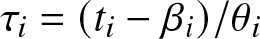 $\tau_i=(t_i-\beta_i)/\theta_i$ and simplifying yields
 \begin{equation*}{
\mathcal{C}\mathcal{J}^{\mathbf{Y}}(t_1,t_2)
= \theta_1\theta_2\,\mathcal{J}^{\mathbf{X}}\!\left(\frac{t_1-\beta_1}{\theta_1},\frac{t_2-\beta_2}{\theta_2}\right)
+\frac{t_1\beta_2 + t_2\beta_1 - \beta_1\beta_2}{2}.
}
\end{equation*}
\begin{equation*}{
\mathcal{C}\mathcal{J}^{\mathbf{Y}}(t_1,t_2)
= \theta_1\theta_2\,\mathcal{J}^{\mathbf{X}}\!\left(\frac{t_1-\beta_1}{\theta_1},\frac{t_2-\beta_2}{\theta_2}\right)
+\frac{t_1\beta_2 + t_2\beta_1 - \beta_1\beta_2}{2}.
}
\end{equation*}This completes the proof.
3. Conditional dynamic negative cumulative extropy
This section examines BDNCEx via a component-wise analysis. Based on this examination, we introduce an alternative formulation known as the conditional dynamic negative cumulative extropy (CDNCEx). Notably, the BDNCEx defined in (2.7) does not uniquely determine the distribution function. To overcome this limitation, we propose a vector-valued version of BDNCEx that captures more detailed information by incorporating its marginal components. Consider the conditional failure model  $
\overline X_i = (X_i \mid X_1 \lt t_1,\, X_2 \lt t_2), \quad i=1,2,$ and assume that
$
\overline X_i = (X_i \mid X_1 \lt t_1,\, X_2 \lt t_2), \quad i=1,2,$ and assume that  $F(t_1,t_2) \gt 0$. The corresponding conditional distribution functions are defined by
  $
F(x_1;t_1,t_2)
= \frac{F(x_1,t_2)}{F(t_1,t_2)}, \quad 0 \lt x_1 \lt t_1,$ and
$
F(x_1;t_1,t_2)
= \frac{F(x_1,t_2)}{F(t_1,t_2)}, \quad 0 \lt x_1 \lt t_1,$ and  $
F(x_2;t_1,t_2)
= \frac{F(t_1,x_2)}{F(t_1,t_2)}, \quad 0 \lt x_2 \lt t_2.
$ In the bivariate setting, vector-valued BDNCEx is defined as
$
F(x_2;t_1,t_2)
= \frac{F(t_1,x_2)}{F(t_1,t_2)}, \quad 0 \lt x_2 \lt t_2.
$ In the bivariate setting, vector-valued BDNCEx is defined as
 \begin{equation}
\mathcal{C} \mathcal{J}^{\textbf X}_{}(t_1,t_2)=\left( \mathcal{C}\mathcal{J}^{\textbf X}_{1{}}(t_1,t_2), \mathcal{C}\mathcal{J}^{\textbf X}_{2{}}(t_1,t_2)\right),
\end{equation}
\begin{equation}
\mathcal{C} \mathcal{J}^{\textbf X}_{}(t_1,t_2)=\left( \mathcal{C}\mathcal{J}^{\textbf X}_{1{}}(t_1,t_2), \mathcal{C}\mathcal{J}^{\textbf X}_{2{}}(t_1,t_2)\right),
\end{equation}where
 \begin{equation}
\mathcal{C} \mathcal{J}^{\textbf X}_{1{}}(t_1,t_2)=\frac{1}{2}\int_0^{t_1}\left(1-\left({F(x_1;t_1t_2)}{}\right)^2\right) dx_1=\frac{1}{2}\int_0^{t_1}\left(1-\left(\frac{F(x_1,t_2)}{F(t_1,t_2)}\right)^2\right) dx_1
\end{equation}
\begin{equation}
\mathcal{C} \mathcal{J}^{\textbf X}_{1{}}(t_1,t_2)=\frac{1}{2}\int_0^{t_1}\left(1-\left({F(x_1;t_1t_2)}{}\right)^2\right) dx_1=\frac{1}{2}\int_0^{t_1}\left(1-\left(\frac{F(x_1,t_2)}{F(t_1,t_2)}\right)^2\right) dx_1
\end{equation}and
 \begin{equation}
\mathcal{C} \mathcal{J}^{\textbf X}_{2{}}(t_1,t_2)=\frac{1}{2}\int_0^{t_1}\left(1-\left({F(x_2;t_1t_2)}{}\right)^2\right) dx_2=\frac{1}{2}\int_0^{t_2}\left(1-\left(\frac{F(t_1,x_2)}{F(t_1,t_2)}\right)^2\right) dx_2
\end{equation}
\begin{equation}
\mathcal{C} \mathcal{J}^{\textbf X}_{2{}}(t_1,t_2)=\frac{1}{2}\int_0^{t_1}\left(1-\left({F(x_2;t_1t_2)}{}\right)^2\right) dx_2=\frac{1}{2}\int_0^{t_2}\left(1-\left(\frac{F(t_1,x_2)}{F(t_1,t_2)}\right)^2\right) dx_2
\end{equation}represent the NCEx of  $(X_i|X_1 \lt t_1,X_2 \lt t_2)$, $i=1,2$. The components of (3.9) are known as CDNCEx. If the RV $\mathbf{X}$ represents the lifetimes of a two-component system, then expressions (3.10) and (3.11) quantify the level of uncertainty associated with the conditional distributions of $X_i$, given that the first component has failed at sometime within the interval $(0, t_1)$ and the second within $(0, t_2)$.
If we assume  $t_2\to\infty$ and $t_1\to\infty$ in (3.10) and (3.11), respectively. Then CDNCEx reduces to univariate DNCEx, defined as
 \begin{equation}
\mathcal{C}\mathcal{J}_i(\mathbf X;t_i)=\begin{cases}
\frac{1}{2}\int_0^{t_1}\left(1-\left(\frac{F_1(x_1)}{F_1(t_1)}\right)^2\right)\,dx_1~~\text{for}~~i=1\\
\frac{1}{2}\int_0^{t_2}\left(1-\left(\frac{F_2(x_2)}{F_2(t_2)}\right)^2\right)\,dx_2~~\text{for}~~i=2.
\end{cases}
\end{equation}
\begin{equation}
\mathcal{C}\mathcal{J}_i(\mathbf X;t_i)=\begin{cases}
\frac{1}{2}\int_0^{t_1}\left(1-\left(\frac{F_1(x_1)}{F_1(t_1)}\right)^2\right)\,dx_1~~\text{for}~~i=1\\
\frac{1}{2}\int_0^{t_2}\left(1-\left(\frac{F_2(x_2)}{F_2(t_2)}\right)^2\right)\,dx_2~~\text{for}~~i=2.
\end{cases}
\end{equation}{ All the subsequent results for CDNCEx are consistent with, and equivalent to, the corresponding univariate case.
Now, we evaluate CDNCEx for BGE distribution.
Example 3.1. Suppose  $\mathbf{X}=(X_1,X_2)$ is a nonnegative RV that follows a BGE distribution, as described in Example 2.1. Since obtaining a closed-form expression for the CDNCEx surface under the BGE distribution is analytically intractable, we compute it numerically and present the resulting 3-D plot in Figure 2. For convenience in graphical representation, the change of variables $t_1 = -\ln x$ and $t_2 = -\ln y$ has been applied.
Numerical plot of  $\mathcal{C}\mathcal{J}^{\mathbf X}_1(t_1,t_2)$ (left) and $\mathcal{C}\mathcal{J}^{\mathbf X}_2(t_1,t_2)$ (right) for BGE distribution for parameters $\beta_1=1.5, \beta_2=1.4$ and $\theta=0.2$ (Example 3.1).

Now we define the bivariate reversed hazard rate (BRHR) and the bivariate expected inactivity time (BEIT) functions, proposed by Roy [Reference Roy27] and Nair and Asha [Reference Nair and Asha19], respectively.
Definition 3.1. Let  $\mathbf{X} = (X_1, X_2)$ be a nonnegative bivariate RV,
(1) the BRHR is defined as the vector
 $
h(t_1, t_2) = \left(h_1(t_1, t_2), \, h_2(t_1, t_2)\right),
$ where
$
h_i(t_1, t_2) = \frac{\partial}{\partial t_i} \log F(t_1, t_2), \quad i = 1, 2.
$ The components
$h_1(t_1, t_2)$ and
$h_2(t_1, t_2)$ represent the instantaneous reversed failure rates corresponding to
$X_1$ and
$X_2$, respectively, conditional on the event
$\{X_1 \lt t_1, X_2 \lt t_2\}$;
$
h(t_1, t_2) = \left(h_1(t_1, t_2), \, h_2(t_1, t_2)\right),
$ where
$
h_i(t_1, t_2) = \frac{\partial}{\partial t_i} \log F(t_1, t_2), \quad i = 1, 2.
$ The components
$h_1(t_1, t_2)$ and
$h_2(t_1, t_2)$ represent the instantaneous reversed failure rates corresponding to
$X_1$ and
$X_2$, respectively, conditional on the event
$\{X_1 \lt t_1, X_2 \lt t_2\}$;(2) the BEIT is defined as the vector
$
\overline{m}(t_1, t_2) = \left(\overline{m}_1(t_1, t_2), \, \overline{m}_2(t_1, t_2)\right),
$ where
$
\overline{m}_i(t_1, t_2) = \mathbb{E}\left(t_i - X_i \mid X_1 \lt t_1, \, X_2 \lt t_2\right), \quad i = 1, 2.
$ That is,
$\overline{m}_i(t_1, t_2)$ represents the expected waiting time elapsed before failure of the
$i$th component, given that both components have failed before
$(t_1, t_2)$. In particular, for
$i = 1$,
$
\overline{m}_1(t_1, t_2) = \frac{1}{F(t_1, t_2)} \int_{0}^{t_1} F(x_1, t_2) \, dx_1,
$ and similarly for
$\overline{m}_2(t_1, t_2)$.


Differentiation of (3.10) with respect to  $t_1$ yields
 \begin{equation}
\frac{\partial}{\partial t_1} \mathcal{C}\mathcal{J}^{\textbf X}_{1{}}(t_1,t_2)=h_1(t_1,t_2)\left[t_1-2 \mathcal{C}\mathcal{J}^{\mathbf X}_1(t_1,t_2)\right].
\end{equation}
\begin{equation}
\frac{\partial}{\partial t_1} \mathcal{C}\mathcal{J}^{\textbf X}_{1{}}(t_1,t_2)=h_1(t_1,t_2)\left[t_1-2 \mathcal{C}\mathcal{J}^{\mathbf X}_1(t_1,t_2)\right].
\end{equation} Similarly, differentiating (3.11) with respect to  $t_2$ gives
 \begin{equation}
\frac{\partial}{\partial t_2} \mathcal{C}\mathcal{J}^{\textbf X}_{2{}}(t_1,t_2)=h_2(t_1,t_2)\left[t_1-2 \mathcal{C}\mathcal{J}^{\mathbf X}_2(t_1,t_2)\right].
\end{equation}
\begin{equation}
\frac{\partial}{\partial t_2} \mathcal{C}\mathcal{J}^{\textbf X}_{2{}}(t_1,t_2)=h_2(t_1,t_2)\left[t_1-2 \mathcal{C}\mathcal{J}^{\mathbf X}_2(t_1,t_2)\right].
\end{equation}Thus, in general, (3.13) and (3.14) can be written as
 \begin{equation}
\frac{\partial}{\partial t_i} \mathcal{C}\mathcal{J}^{\textbf X}_{i{}}(t_1,t_2)=h_i(t_1,t_2)\left[t_i-2 \mathcal{C}\mathcal{J}^{\mathbf X}_i(t_1,t_2)\right],\quad i=1,2.
\end{equation}
\begin{equation}
\frac{\partial}{\partial t_i} \mathcal{C}\mathcal{J}^{\textbf X}_{i{}}(t_1,t_2)=h_i(t_1,t_2)\left[t_i-2 \mathcal{C}\mathcal{J}^{\mathbf X}_i(t_1,t_2)\right],\quad i=1,2.
\end{equation}The subsequent theorem establishes a lower bound of CDNCEx.
Theorem 3.1 Assume a nonnegative RV  $\textbf X$ having BEIT $\overline{m}_i(t_1,t_2)$. Then for $t_1,t_2 \gt 0$,
 \begin{align*}
\mathcal{C}\mathcal{J}^{\mathbf X}_i(t_1,t_2)\geq \frac{1}{2} \left(t_i- \overline{m}_i(t_1,t_2)\right),~i=1,2.
\end{align*}
\begin{align*}
\mathcal{C}\mathcal{J}^{\mathbf X}_i(t_1,t_2)\geq \frac{1}{2} \left(t_i- \overline{m}_i(t_1,t_2)\right),~i=1,2.
\end{align*}Proof. Since  $0\leq \frac{F(x_1,t_2)}{F(t_1,t_2)}\leq 1$ $\forall$ $x_1\leq t_1$ and for all $t_1,t_2\geq 0$. This yields
 \begin{align*}
\frac{1}{2}\int_0^{t_1}\left(1-\left(\frac{F(x_1,t_2)}{ F(t_1,t_2)}\right)^2\right)dx_1&\geq \frac{1}{2}\int_0^{t_1}\left(1-\frac{F(x_1,t_2)}{F(t_1,t_2)}\right) dx_1\\
&=\frac{1}{2}\left(t_1-\overline{m}_1(t_1,t_2)\right).
\end{align*}
\begin{align*}
\frac{1}{2}\int_0^{t_1}\left(1-\left(\frac{F(x_1,t_2)}{ F(t_1,t_2)}\right)^2\right)dx_1&\geq \frac{1}{2}\int_0^{t_1}\left(1-\frac{F(x_1,t_2)}{F(t_1,t_2)}\right) dx_1\\
&=\frac{1}{2}\left(t_1-\overline{m}_1(t_1,t_2)\right).
\end{align*} A similar result holds for  $i=2$.
For a rigorous probabilistic characterization of CDNCEx, consider the following definition
 \begin{equation}
\omega_1^{(2)}(c,d;t_2)=\int_c^d F(x_1,t_2)dx_1,
\end{equation}
\begin{equation}
\omega_1^{(2)}(c,d;t_2)=\int_c^d F(x_1,t_2)dx_1,
\end{equation}where  $c,d\in\mathbb{R}$ and $0 \lt c\leq d$. It can be seen that $\frac{\partial}{\partial t_1}\omega^{(2)}_1(c;t_1,t_2)=F(t_1,t_2).$
Now, we evaluate the CDNCEx of some distributions. The importance of  $\omega_1^{(2)}(c,d;t_2)$ stems from the relationship between its partial derivative and the CDF of $\textbf X$. Analogously, we may define
 \begin{align*}
\omega_2^{(2)}(c,d;t_1)=\int_c^d F(t_1,x_2)dx_2.
\end{align*}
\begin{align*}
\omega_2^{(2)}(c,d;t_1)=\int_c^d F(t_1,x_2)dx_2.
\end{align*} For  $i = 1, 2$, the following result establishes a fundamental relationship between $\mathcal{J}^{\textbf X}_{i{}}(t_1,t_2)$ and $ \omega_i^{(2)}(c,d;t_i)$.
Theorem 3.2 Let  $\textbf X$ be a nonnegative bivariate RV. For all $t_i, t_j \geq 0~ (i, j \in \{1, 2\})$, we obtain
 \begin{align*}
E\left[\mathcal \omega_i^{(2)}(X_i;t_1,t_2)|X_1 \lt t_1,X_2 \lt t_2\right]=2\left(\frac{t_i}{2}- \mathcal{C} {\mathcal{J}}^{\textbf X}_{i}(t_1,t_2)\right)F(t_1,t_2).
\end{align*}
\begin{align*}
E\left[\mathcal \omega_i^{(2)}(X_i;t_1,t_2)|X_1 \lt t_1,X_2 \lt t_2\right]=2\left(\frac{t_i}{2}- \mathcal{C} {\mathcal{J}}^{\textbf X}_{i}(t_1,t_2)\right)F(t_1,t_2).
\end{align*}Proof. We begin by establishing the case for  $i=1$. From (3.10), we derive
 \begin{align*}
\mathcal{C} {\mathcal{J}}^{\textbf X}_{1}(t_1,t_2)&=\frac{t_1}{2}-\frac{1}{2F^2(t_1,t_2)}\int_0^{t_1}F^2(x_1,t_2)dx_1\\
&=\frac{t_1}{2}-\frac{1}{2F^2(t_1,t_2)}\int_0^{t_1}\left(\int_0^{x_1}\frac{\partial}{\partial u}F(u,t_2)du\right)F(x_1,t_2)dx_1\\
&=\frac{t_1}{2}-\frac{1}{2F^2(t_1,t_2)}\int_0^{t_1}\frac{\partial F(u,t_2)}{\partial u}\left(\int_u^{t_1}F(x_1,t_2)dx_1\right)du\\
&=\frac{t_1}{2}-\frac{1}{2F^2(t_1,t_2)}F(t_1,t_2)E\left[\int_{X_1}^{t_1}F(u,t_2)du|X_1 \lt t_1,X_2 \lt t_2\right]\\
&=\frac{t_1}{2}-\frac{1}{2F(t_1,t_2)}E\left[\omega_1^{(2)}(X_1,t_1;t_2)|X_1 \lt t_1,X_2 \lt t_2\right],
\end{align*}
\begin{align*}
\mathcal{C} {\mathcal{J}}^{\textbf X}_{1}(t_1,t_2)&=\frac{t_1}{2}-\frac{1}{2F^2(t_1,t_2)}\int_0^{t_1}F^2(x_1,t_2)dx_1\\
&=\frac{t_1}{2}-\frac{1}{2F^2(t_1,t_2)}\int_0^{t_1}\left(\int_0^{x_1}\frac{\partial}{\partial u}F(u,t_2)du\right)F(x_1,t_2)dx_1\\
&=\frac{t_1}{2}-\frac{1}{2F^2(t_1,t_2)}\int_0^{t_1}\frac{\partial F(u,t_2)}{\partial u}\left(\int_u^{t_1}F(x_1,t_2)dx_1\right)du\\
&=\frac{t_1}{2}-\frac{1}{2F^2(t_1,t_2)}F(t_1,t_2)E\left[\int_{X_1}^{t_1}F(u,t_2)du|X_1 \lt t_1,X_2 \lt t_2\right]\\
&=\frac{t_1}{2}-\frac{1}{2F(t_1,t_2)}E\left[\omega_1^{(2)}(X_1,t_1;t_2)|X_1 \lt t_1,X_2 \lt t_2\right],
\end{align*}proving the result. The last equality is obtained using (3.16). The proof for  $i=2$ follows similarly.
Definition 3.2. The bivariate RV  $\mathbf X$ is classified as increasing (decreasing) in CDNCEx if $ \mathcal{C}\mathcal{J}^{\textbf X}_{i{}}(t_1,t_2)$ is an increasing (decreasing) function of $t_i$, where $i=1,2.$
The following theorem establishes that, under specific conditions on  $ \mathcal{C}\mathcal{J}^{\textbf X}_{i{}}(t_1,t_2)$, the components of the BRHR function for $\mathbf{X}$ exhibit an increasing (or decreasing) trend.
Theorem 3.3 A nonnegative RV  $\textbf X$ is said to have increasing (decreasing) in CDNCEx if and only if
 \begin{align*}
\mathcal{C}\mathcal{J}^{\mathbf X}_i(t_1,t_2)\leq(\geq) \frac{t_i}{2}, ~i=1,2.
\end{align*}
\begin{align*}
\mathcal{C}\mathcal{J}^{\mathbf X}_i(t_1,t_2)\leq(\geq) \frac{t_i}{2}, ~i=1,2.
\end{align*}Proof. From (3.15), we have
 \begin{align*}
\frac{\partial}{\partial t_i} \mathcal{C}\mathcal{J}^{\textbf X}_{i{}}(t_1,t_2)=h_i(t_1,t_2)\left[t_i-2 \mathcal{C}\mathcal{J}^{\mathbf X}_i(t_1,t_2)\right].
\end{align*}
\begin{align*}
\frac{\partial}{\partial t_i} \mathcal{C}\mathcal{J}^{\textbf X}_{i{}}(t_1,t_2)=h_i(t_1,t_2)\left[t_i-2 \mathcal{C}\mathcal{J}^{\mathbf X}_i(t_1,t_2)\right].
\end{align*} If  $\mathcal{C}\mathcal{J}^{\mathbf X}_i(t_1,t_2)$ is increasing (decreasing) in $t_i$, then $\frac{\partial}{\partial t_i}\mathcal{C}\mathcal{J}^{\mathbf X}_i(t_1,t_2)\geq (\leq) ~0$. It follows that
 \begin{align*}
h_i(t_1,t_2)\left[t_i-2 \mathcal{C}\mathcal{J}^{\mathbf X}_i(t_1,t_2)\right]\geq (\leq) ~0,
\end{align*}
\begin{align*}
h_i(t_1,t_2)\left[t_i-2 \mathcal{C}\mathcal{J}^{\mathbf X}_i(t_1,t_2)\right]\geq (\leq) ~0,
\end{align*}but  $h_i(t_1,t_2)\geq 0$, this yields
 \begin{align*}
\mathcal{C}\mathcal{J}^{\mathbf X}_i(t_1,t_2)\leq (\geq)~ \frac{t_i}{2}.
\end{align*}
\begin{align*}
\mathcal{C}\mathcal{J}^{\mathbf X}_i(t_1,t_2)\leq (\geq)~ \frac{t_i}{2}.
\end{align*}The converse is straightforward and is therefore omitted.
Theorem 3.4 Let  $\mathbf X=(X_1,X_2)$ be a nonnegative absolutely continuous RV with joint PDF $f(x_1,x_2) \gt 0$ on $(0,t_1)\times(0,t_2)$. Then
 \begin{align*}
\mathcal{C}\mathcal{J}^{\mathbf X}_i(t_1,t_2) \lt \frac{t_i}{2}, \quad i=1,2.
\end{align*}
\begin{align*}
\mathcal{C}\mathcal{J}^{\mathbf X}_i(t_1,t_2) \lt \frac{t_i}{2}, \quad i=1,2.
\end{align*}Proof. Since  $\mathbf X$ is nonnegative and absolutely continuous with joint density $f$, for any $0 \lt x_1 \lt t_1$ and $t_2 \gt 0$,
 \begin{equation*}
F(x_1,t_2)=\int_0^{x_1}\int_0^{t_2} f(u,v)\,dv\,du \gt 0,
\end{equation*}
\begin{equation*}
F(x_1,t_2)=\int_0^{x_1}\int_0^{t_2} f(u,v)\,dv\,du \gt 0,
\end{equation*}and
 \begin{equation*}
F(t_1,t_2)-F(x_1,t_2)
= \int_{x_1}^{t_1}\int_0^{t_2} f(u,v)\,dv\,du \gt 0.
\end{equation*}
\begin{equation*}
F(t_1,t_2)-F(x_1,t_2)
= \int_{x_1}^{t_1}\int_0^{t_2} f(u,v)\,dv\,du \gt 0.
\end{equation*}Hence,
 \begin{equation*}
0 \lt F(x_1,t_2) \lt F(t_1,t_2)\implies 0 \lt F(x_1;t_1,t_2) \lt 1.
\end{equation*}
\begin{equation*}
0 \lt F(x_1,t_2) \lt F(t_1,t_2)\implies 0 \lt F(x_1;t_1,t_2) \lt 1.
\end{equation*} Integrating both sides over  $(0,t_1)$ gives
 \begin{equation*}
\int_0^{t_1} \bigl(1 - F^2(x_1;t_1,t_2)\bigr)\,dx_1 \lt t_1.
\end{equation*}
\begin{equation*}
\int_0^{t_1} \bigl(1 - F^2(x_1;t_1,t_2)\bigr)\,dx_1 \lt t_1.
\end{equation*} The argument for  $i=2$ is identical. This completes the proof.
The following theorem establishes that the CDNCEx fails to remain invariant under non-singular transformations.
Theorem 3.5 Consider a nonnegative RV  $\textbf X$ with joint CDF $F(x_1,x_2)$. Let $Y_i=\Phi_i(X_i),~i=1,2$, where $\Phi_i$ is an injective and differentiable function.
Then, for  $i=1,$
 \begin{align*}
\mathcal{C} \mathcal{J}^{(\Phi(X_1),\Phi(X_2))}_{1{}}(t_1,t_2)=\begin{cases}&\frac{1}{2}\int_{\Phi_1^{-1}(0)}^{\Phi_1^{-1}(t_1)} \left(1-\left(\frac{F(x_1,\Phi_2^{-1}(t_2))}{F(\Phi_1^{-1}(t_1),\Phi_2^{-1}(t_2)}\right)^2\right)\Phi_1'(x_1)dx_1,\\
&~~~\text{if}~\Phi_1~\text{is strictly increasing.}\\
&\frac{1}{2}\int_{\Phi_1^{-1}(t_1)}^{\Phi_1^{-1}(0)} \left(1-\left(\frac{\bar{F}(x_1,\Phi_1^{-1}(t_2))}{\bar{F}(\Phi_1^{-1}(t_1),\Phi_1^{-1}(t_2))}\right)^2\right)\Phi_1'(x_1)dx_1,\\
&~~~\text{if}~\Phi_1~\text{is strictly decreasing.}
\end{cases}
\end{align*}
\begin{align*}
\mathcal{C} \mathcal{J}^{(\Phi(X_1),\Phi(X_2))}_{1{}}(t_1,t_2)=\begin{cases}&\frac{1}{2}\int_{\Phi_1^{-1}(0)}^{\Phi_1^{-1}(t_1)} \left(1-\left(\frac{F(x_1,\Phi_2^{-1}(t_2))}{F(\Phi_1^{-1}(t_1),\Phi_2^{-1}(t_2)}\right)^2\right)\Phi_1'(x_1)dx_1,\\
&~~~\text{if}~\Phi_1~\text{is strictly increasing.}\\
&\frac{1}{2}\int_{\Phi_1^{-1}(t_1)}^{\Phi_1^{-1}(0)} \left(1-\left(\frac{\bar{F}(x_1,\Phi_1^{-1}(t_2))}{\bar{F}(\Phi_1^{-1}(t_1),\Phi_1^{-1}(t_2))}\right)^2\right)\Phi_1'(x_1)dx_1,\\
&~~~\text{if}~\Phi_1~\text{is strictly decreasing.}
\end{cases}
\end{align*}Proof. Assume that  $\Phi_i$ is strictly increasing. Then, by monotonicity of the transformation, we have
 \begin{align*}
F_{\mathbf Y}(y_1,t_2)
&= P(Y_1 \lt y_1, Y_2 \lt t_2)
= P\big(X_1 \lt \Phi_1^{-1}(y_1),\, X_2 \lt \Phi_2^{-1}(t_2)\big)
= F_{\mathbf X}\big(\Phi_1^{-1}(y_1), \Phi_2^{-1}(t_2)\big),\\~\text{and}~
F_{\mathbf Y}(t_1,t_2)
&= F_{\mathbf X}\big(\Phi_1^{-1}(t_1), \Phi_2^{-1}(t_2)\big).
\end{align*}
\begin{align*}
F_{\mathbf Y}(y_1,t_2)
&= P(Y_1 \lt y_1, Y_2 \lt t_2)
= P\big(X_1 \lt \Phi_1^{-1}(y_1),\, X_2 \lt \Phi_2^{-1}(t_2)\big)
= F_{\mathbf X}\big(\Phi_1^{-1}(y_1), \Phi_2^{-1}(t_2)\big),\\~\text{and}~
F_{\mathbf Y}(t_1,t_2)
&= F_{\mathbf X}\big(\Phi_1^{-1}(t_1), \Phi_2^{-1}(t_2)\big).
\end{align*} Using the transformation  $y_i = \Phi_i(x_i)$, we obtain $dy_1 = \Phi_1'(x_1)\,dx_1$. Hence,
 \begin{align*}
\mathcal{C}\mathcal{J}^{(\Phi(X_1),\Phi(X_2))}_{1}(t_1,t_2)
= \frac{1}{2}\int_{\Phi_1^{-1}(0)}^{\Phi_1^{-1}(t_1)}
\left(1 - \left(\frac{F(x_1,\Phi_2^{-1}(t_2))}{F(\Phi_1^{-1}(t_1),\Phi_2^{-1}(t_2))}\right)^2\right)
\Phi_1'(x_1)\,dx_1.
\end{align*}
\begin{align*}
\mathcal{C}\mathcal{J}^{(\Phi(X_1),\Phi(X_2))}_{1}(t_1,t_2)
= \frac{1}{2}\int_{\Phi_1^{-1}(0)}^{\Phi_1^{-1}(t_1)}
\left(1 - \left(\frac{F(x_1,\Phi_2^{-1}(t_2))}{F(\Phi_1^{-1}(t_1),\Phi_2^{-1}(t_2))}\right)^2\right)
\Phi_1'(x_1)\,dx_1.
\end{align*} A similar argument holds when  $\Phi_i$ is strictly decreasing.
The following result describes the affine transformation property of the CDNCEx measure.
Theorem 3.6 Let  $\mathbf{X}$ and $\mathbf{Y}$ be nonnegative RVs. If $Y_i=\mu_iX_i+\eta_i,~\mu_i \gt 0,~\eta_i\geq0$ for $i=1,2$, then
 \begin{equation*}{\mathcal{C}\mathcal{J}^{\textbf Y}_{i{}}(t_1,t_2)= \mu_i\,\mathcal{C}\mathcal{J}^{\mathbf X}_{i}\!\Big(\frac{t_1-\eta_1}{\mu_1},\frac{t_2-\eta_2}{\mu_2}\Big)
+\frac{\eta_i}{2}.}\end{equation*}
\begin{equation*}{\mathcal{C}\mathcal{J}^{\textbf Y}_{i{}}(t_1,t_2)= \mu_i\,\mathcal{C}\mathcal{J}^{\mathbf X}_{i}\!\Big(\frac{t_1-\eta_1}{\mu_1},\frac{t_2-\eta_2}{\mu_2}\Big)
+\frac{\eta_i}{2}.}\end{equation*}Proof. From (3.10), we have
 \begin{equation*}
\mathcal{C}\mathcal{J}^{\mathbf Y}_{1}(t_1,t_2)
=\frac{1}{2}\int_{0}^{t_1}\left(1-\left(\frac{F_{\mathbf Y}(y_1,t_2)}{F_{\mathbf Y}(t_1,t_2)}\right)^2\right)\,dy_1.
\end{equation*}
\begin{equation*}
\mathcal{C}\mathcal{J}^{\mathbf Y}_{1}(t_1,t_2)
=\frac{1}{2}\int_{0}^{t_1}\left(1-\left(\frac{F_{\mathbf Y}(y_1,t_2)}{F_{\mathbf Y}(t_1,t_2)}\right)^2\right)\,dy_1.
\end{equation*} Applying the transformation  $Y_i=\mu_i X_i+\eta_i$ yields
 \begin{equation*}
F_{\mathbf Y}(y_1,t_2)=F_{\mathbf X}\!\Big(\frac{y_1-\eta_1}{\mu_1},\frac{t_2-\eta_2}{\mu_2}\Big).
\end{equation*}
\begin{equation*}
F_{\mathbf Y}(y_1,t_2)=F_{\mathbf X}\!\Big(\frac{y_1-\eta_1}{\mu_1},\frac{t_2-\eta_2}{\mu_2}\Big).
\end{equation*} Set  $x_1=(y_1-\eta_1)/\mu_1$, so $y_1=\mu_1 x_1+\eta_1$ and $dy_1=\mu_1\,dx_1$. Hence
 \begin{equation*}
\mathcal{C}\mathcal{J}^{\mathbf Y}_{1}(t_1,t_2)
=\frac{\mu_1}{2}\int_{-\eta_1/\mu_1}^{(t_1-\eta_1)/\mu_1}
\left(1-\left(\frac{F_{\mathbf X}\big(x_1,(t_2-\eta_2)/\mu_2\big)}{F_{\mathbf X}\big((t_1-\eta_1)/\mu_1,(t_2-\eta_2)/\mu_2\big)}\right)^2\right)\,dx_1.
\end{equation*}
\begin{equation*}
\mathcal{C}\mathcal{J}^{\mathbf Y}_{1}(t_1,t_2)
=\frac{\mu_1}{2}\int_{-\eta_1/\mu_1}^{(t_1-\eta_1)/\mu_1}
\left(1-\left(\frac{F_{\mathbf X}\big(x_1,(t_2-\eta_2)/\mu_2\big)}{F_{\mathbf X}\big((t_1-\eta_1)/\mu_1,(t_2-\eta_2)/\mu_2\big)}\right)^2\right)\,dx_1.
\end{equation*}It follows that
 \begin{equation*}
{\;
\mathcal{C}\mathcal{J}^{\mathbf Y}_{1}(t_1,t_2)
= \mu_1\,\mathcal{C}\mathcal{J}^{\mathbf X}_{1}\!\Big(\frac{t_1-\eta_1}{\mu_1},\frac{t_2-\eta_2}{\mu_2}\Big)
+\frac{\eta_1}{2}\; }.
\end{equation*}
\begin{equation*}
{\;
\mathcal{C}\mathcal{J}^{\mathbf Y}_{1}(t_1,t_2)
= \mu_1\,\mathcal{C}\mathcal{J}^{\mathbf X}_{1}\!\Big(\frac{t_1-\eta_1}{\mu_1},\frac{t_2-\eta_2}{\mu_2}\Big)
+\frac{\eta_1}{2}\; }.
\end{equation*} Following the same steps used for  $i=1$, we can also establish the case for $i=2$.
We now demonstrate that the affine transformation preserves the monotonicity of  $\mathcal{C}\mathcal{J}^{\textbf X}_{i{}}(t_1,t_2)$, as formalized in the result below.
Theorem 3.7 Assume two nonnegative bivariate RVs  $\textbf X$ and $\textbf Y$, where $Y_i=\mu_iX_i+\eta_i$ with $\mu_i \gt 0$ and $\eta_i\geq 0$ for $i=1,2$. Then $\mathcal{C}\mathcal{J}^{\textbf Y}_{i{}}(t_1,t_2)$ is increasing in $t_i$ if and only if $ \mathcal{C}\mathcal{J}^{\textbf X}_{i{}}(t_1,t_2)$ is increasing in $t_i$.
Proof. Let  $Y_i=\mu_iX_i+\eta_i$ with $\mu_i \gt 0$ and $\eta_i\ge0$. For $t_i\ge\eta_i$, the joint CDF of $\mathbf Y$ satisfies
 \begin{equation*}
F_{\mathbf Y}(t_1,t_2)=P(Y_1\le t_1,Y_2\le t_2)=F_{\mathbf X}\!\left(\frac{t_1-\eta_1}{\mu_1},\frac{t_2-\eta_2}{\mu_2}\right).
\end{equation*}
\begin{equation*}
F_{\mathbf Y}(t_1,t_2)=P(Y_1\le t_1,Y_2\le t_2)=F_{\mathbf X}\!\left(\frac{t_1-\eta_1}{\mu_1},\frac{t_2-\eta_2}{\mu_2}\right).
\end{equation*}Hence, from Theorem 3.5, we have
 \begin{equation}
\mathcal{C}\mathcal{J}^{\mathbf Y}_{i}(t_1,t_2)
=\mu_i\,\mathcal{C}\mathcal{J}^{\mathbf X}_{i}\!\left(\frac{t_1-\eta_1}{\mu_1},\frac{t_2-\eta_2}{\mu_2}\right),
\qquad t_i\ge \eta_i.
\end{equation}
\begin{equation}
\mathcal{C}\mathcal{J}^{\mathbf Y}_{i}(t_1,t_2)
=\mu_i\,\mathcal{C}\mathcal{J}^{\mathbf X}_{i}\!\left(\frac{t_1-\eta_1}{\mu_1},\frac{t_2-\eta_2}{\mu_2}\right),
\qquad t_i\ge \eta_i.
\end{equation} Let  $\phi_i(t_i)=\dfrac{t_i-\eta_i}{\mu_i}$, so that $\phi_i'(t_i)=1/\mu_i \gt 0$ and, let $s_i=\phi_i(t_i)$. Differentiating (3.17) with respect to $t_i$ gives
 \begin{equation}
\frac{\partial}{\partial t_i}\mathcal{C}\mathcal{J}^{\mathbf Y}_{i}(t_1,t_2)
=\mu_i\frac{\partial}{\partial s_i}\mathcal{C}\mathcal{J}^{\mathbf X}_{i}\left(\phi_1(t_1),\phi_2(t_2)\right)\phi_i'(t_i)
=\frac{\partial}{\partial s_i}\mathcal{C}\mathcal{J}^{\mathbf X}_{i}\left(s_1,s_2\right).
\end{equation}
\begin{equation}
\frac{\partial}{\partial t_i}\mathcal{C}\mathcal{J}^{\mathbf Y}_{i}(t_1,t_2)
=\mu_i\frac{\partial}{\partial s_i}\mathcal{C}\mathcal{J}^{\mathbf X}_{i}\left(\phi_1(t_1),\phi_2(t_2)\right)\phi_i'(t_i)
=\frac{\partial}{\partial s_i}\mathcal{C}\mathcal{J}^{\mathbf X}_{i}\left(s_1,s_2\right).
\end{equation} Hence,  $\mathcal{C}\mathcal{J}^{\mathbf Y}_{i}(t_1,t_2)$ is increasing in $t_i$ if and only if $\mathcal{C}\mathcal{J}^{\mathbf X}_{i}(t_1,t_2)$ is increasing in $t_i$.
The following theorem establishes that CDNCEx uniquely determines the distribution function.
Theorem 3.8 Let  $\mathbf{X}$ be a nonnegative absolutely continuous bivariate RV with PDF $f(x_1,x_2) \gt 0$ on $(0,t_1)\times(0,t_2)$. Then, CDNCEx uniquely determines the underlying CDF.
Proof. Assume that  $\mathbf{X}$ and $\mathbf{Y}$ are two RVs with joint CDFs $F$ and $G$, respectively, and let ${h}^{\mathbf{X}}_i(t_1, t_2) \gt 0$ and ${h}^{\mathbf{Y}}_i(t_1, t_2) \gt 0$ denote the components of their respective BRHR. Suppose that
 \begin{equation}
\mathcal{C}\mathcal{J}^{\mathbf{X}}_{i}(t_1, t_2) = \mathcal{C}\mathcal{J}^{\mathbf{Y}}_{i}(t_1, t_2).
\end{equation}
\begin{equation}
\mathcal{C}\mathcal{J}^{\mathbf{X}}_{i}(t_1, t_2) = \mathcal{C}\mathcal{J}^{\mathbf{Y}}_{i}(t_1, t_2).
\end{equation} Differentiating (3.19) with respect to  $t_1$ and simplifying, we obtain
 \begin{align*}
h^{\mathbf{X}}_i(t_1, t_2) \left[t_i - 2\,\mathcal{C}\mathcal{J}^{\mathbf{X}}_{i}(t_1, t_2)\right]
= h^{\mathbf{Y}}_i(t_1, t_2) \left[t_i - 2\,\mathcal{C}\mathcal{J}^{\mathbf{Y}}_{i}(t_1, t_2)\right].
\end{align*}
\begin{align*}
h^{\mathbf{X}}_i(t_1, t_2) \left[t_i - 2\,\mathcal{C}\mathcal{J}^{\mathbf{X}}_{i}(t_1, t_2)\right]
= h^{\mathbf{Y}}_i(t_1, t_2) \left[t_i - 2\,\mathcal{C}\mathcal{J}^{\mathbf{Y}}_{i}(t_1, t_2)\right].
\end{align*}Now, using Theorem 3.4, we obtain,
 \begin{align*}
{h}^{\mathbf{X}}_i(t_1, t_2) = {h}^{\mathbf{Y}}_i(t_1, t_2).
\end{align*}
\begin{align*}
{h}^{\mathbf{X}}_i(t_1, t_2) = {h}^{\mathbf{Y}}_i(t_1, t_2).
\end{align*}Consequently, the result follows from the fundamental principle that the vector-valued BRHR uniquely characterizes the underlying CDF (see [Reference Roy27]).
The following result establishes that CDNCEx reduces to univariate NCEx when the components are independent.
Theorem 3.9 Let  $\mathbf X$ be a nonnegative bivariate RV $\mathbf{X}$ with PDF $f(x_1,x_2) \gt 0$ on $(0,t_1)\times(0,t_2)$. Then
 \begin{equation}
\mathcal{C}\mathcal{J}^{\mathbf{X}}_i(t_1, t_2) = \mathcal{C}\mathcal{J}(X_i; t_i), \quad i = 1, 2,
\end{equation}
\begin{equation}
\mathcal{C}\mathcal{J}^{\mathbf{X}}_i(t_1, t_2) = \mathcal{C}\mathcal{J}(X_i; t_i), \quad i = 1, 2,
\end{equation}if and only if  $X_1$ and $X_2$ are independent.
Proof. Assume that (3.20) holds. Then we have
 \begin{align*}
\frac{1}{2} \int_0^{t_1} \left(1 - \left(\frac{F(x_1, t_2)}{F(t_1, t_2)}\right)^2 \right) dx_1
= \frac{1}{2} \int_0^{t_1} \left(1 - \left(\frac{F_1(x_1)}{F_1(t_1)}\right)^2 \right) dx_1.
\end{align*}
\begin{align*}
\frac{1}{2} \int_0^{t_1} \left(1 - \left(\frac{F(x_1, t_2)}{F(t_1, t_2)}\right)^2 \right) dx_1
= \frac{1}{2} \int_0^{t_1} \left(1 - \left(\frac{F_1(x_1)}{F_1(t_1)}\right)^2 \right) dx_1.
\end{align*} Differentiating both sides with respect to  $t_1$, we obtain
 \begin{equation}
h_1(t_1, t_2) \left[t_1 - 2\,\mathcal{C}\mathcal{J}^{\mathbf{X}}_{1}(t_1, t_2)\right]
= h_1(t_1) \left[t_1 - 2\,\mathcal{C}\mathcal{J}(X_1; t_1)\right],
\end{equation}
\begin{equation}
h_1(t_1, t_2) \left[t_1 - 2\,\mathcal{C}\mathcal{J}^{\mathbf{X}}_{1}(t_1, t_2)\right]
= h_1(t_1) \left[t_1 - 2\,\mathcal{C}\mathcal{J}(X_1; t_1)\right],
\end{equation}where  $h_i(t_1, t_2)$ denotes the component of the BRHR of $\mathbf{X}$, and $h_1(t_1) = \frac{d}{dt_1} \log F_1(t_1)$ represents the univariate reversed hazard rate of $X_1$. Therefore, from Theorem 3.4 and (3.21), we get
 \begin{align*}
\frac{\partial}{\partial t_1} h_1(t_1, t_2)
= \frac{\partial}{\partial t_1} h_1(t_1).
\end{align*}
\begin{align*}
\frac{\partial}{\partial t_1} h_1(t_1, t_2)
= \frac{\partial}{\partial t_1} h_1(t_1).
\end{align*}Hence
 \begin{equation}
\frac{\partial}{\partial t_1} \log F(t_1, t_2)
= \frac{\partial}{\partial t_1} \log F_1(t_1).
\end{equation}
\begin{equation}
\frac{\partial}{\partial t_1} \log F(t_1, t_2)
= \frac{\partial}{\partial t_1} \log F_1(t_1).
\end{equation} Integrating both sides of (3.22) with respect to  $t_1$ (for fixed $t_2$), we obtain
 \begin{equation}
\log F(t_1, t_2) = \log F_1(t_1) + \varphi(t_2),
\end{equation}
\begin{equation}
\log F(t_1, t_2) = \log F_1(t_1) + \varphi(t_2),
\end{equation}where  $ \varphi(t_2)$ is a function depending only on $t_2$. Exponentiating both sides of (3.23) yields
 \begin{equation}
F(t_1, t_2) = F_1(t_1)\, e^{\varphi(t_2)}.
\end{equation}
\begin{equation}
F(t_1, t_2) = F_1(t_1)\, e^{\varphi(t_2)}.
\end{equation} Let  $g(t_2) = e^{\varphi (t_2)} \gt 0$, so that $F(t_1, t_2) = F_1(t_1)\, g(t_2)$. Using the definition of the second marginal, we have
 \begin{equation*}
F_2(t_2) = \lim_{t_1 \to \infty} F(t_1, t_2) = \lim_{t_1 \to \infty} F_1(t_1)\, g(t_2) = g(t_2),
\end{equation*}
\begin{equation*}
F_2(t_2) = \lim_{t_1 \to \infty} F(t_1, t_2) = \lim_{t_1 \to \infty} F_1(t_1)\, g(t_2) = g(t_2),
\end{equation*}since  $\lim_{t_1 \to \infty} F_1(t_1) = 1$. Substituting this result into (3.24) gives
 \begin{equation*}
F(t_1, t_2) = F_1(t_1) F_2(t_2).
\end{equation*}
\begin{equation*}
F(t_1, t_2) = F_1(t_1) F_2(t_2).
\end{equation*}The converse part is straightforward and is therefore omitted.
Next, we define a new stochastic ordering derived from CDNCEx.
Definition 3.3. Consider two nonnegative bivariate RVs  $\mathbf{X}$ and $\mathbf{Y}$. We say that $\mathbf{X}$ is greater (or less) than $\mathbf{Y}$ in CDNCEx, denoted as $\mathbf{X} \geq_{\text{CDNCEx}} (\leq_{\text{CDNCEx}}) \mathbf{Y}$, if for all $t_1,t_2 \gt 0$ and for $i = 1,2$, the following inequality holds
 \begin{equation*} \mathcal{C}\mathcal{J}^{\mathbf X}_{i{}}(t_1, t_2) \geq (\leq) \mathcal{C}\mathcal{J}^{\mathbf Y}_{i{}}( t_1, t_2).\end{equation*}
Subsequently, we show that the usual stochastic order preserves the stochastic order based on CDNCEx.
Theorem 3.10 Assume two nonnegative RVs  $\mathbf{X}$ and $\mathbf{Y}$. Define the conditional random variables
  $
\overline{X}_i = (X_i \mid X_1 \lt t_1, X_2 \lt t_2)~\text{and}~\overline{Y}_i = (Y_i \mid Y_1 \lt t_1, Y_2 \lt t_2).
$ If
$
\overline{X}_i = (X_i \mid X_1 \lt t_1, X_2 \lt t_2)~\text{and}~\overline{Y}_i = (Y_i \mid Y_1 \lt t_1, Y_2 \lt t_2).
$ If  $\overline X_i\geq_{st}(\leq_{st})\overline Y_i$, then $\mathbf X\geq_{CDNCEx}(\leq_{CDNCEx}) \mathbf Y,~i=1,2.$
Proof. For  $i=1$, if $\overline X_1\geq_{st}(\leq_{st})\overline Y_1$, then $\frac{F(x_1,t_2)}{F(t_1,t_2)}\leq(\geq) \frac{G(x_1,t_2)}{G(t_1,t_2)}$. Therefore, we have $ \mathcal{C}\mathcal{J}^{\textbf X}_{1{}}(t_1,t_2)\geq(\leq) \mathcal{C} \mathcal{J}^{\textbf Y}_{1{}}(t_1,t_2)$. Similarly, the rest of the part follows.
In support of Theorem 3.10, we consider the following example.
Example 3.2. Consider two nonnegative bivariate RVs  $\mathbf X$ and $\mathbf Y$ have respective CDFs
 \begin{align*}
F_{\mathbf X}(x_1,x_2)=\left(1-e^{-\mu_1 x_1}\right)^{0.5}+\left(1-e^{-\mu_2 x_2}\right)^{0.5}-\left(1-e^{-\mu_1 x_1-\mu_2 x_2}\right)^{0.5}, x_1, x_2\geq 0,~\mu_1,\mu_2 \gt 0,~~\text{and}
\end{align*}
\begin{align*}
F_{\mathbf X}(x_1,x_2)=\left(1-e^{-\mu_1 x_1}\right)^{0.5}+\left(1-e^{-\mu_2 x_2}\right)^{0.5}-\left(1-e^{-\mu_1 x_1-\mu_2 x_2}\right)^{0.5}, x_1, x_2\geq 0,~\mu_1,\mu_2 \gt 0,~~\text{and}
\end{align*} \begin{align*}
F_{\mathbf Y}(x_1,x_2)=\left(1-e^{-\mu_3 x_1}\right)^{0.5}+\left(1-e^{-\mu_4 x_2}\right)^{0.5}-\left(1-e^{-\mu_3 x_1-\mu_4 x_2}\right)^{0.5}, x_1, x_2\geq 0,~\mu_3,\mu_4 \gt 0,
\end{align*}
\begin{align*}
F_{\mathbf Y}(x_1,x_2)=\left(1-e^{-\mu_3 x_1}\right)^{0.5}+\left(1-e^{-\mu_4 x_2}\right)^{0.5}-\left(1-e^{-\mu_3 x_1-\mu_4 x_2}\right)^{0.5}, x_1, x_2\geq 0,~\mu_3,\mu_4 \gt 0,
\end{align*} with corresponding marginal CDFs  $F_{X_1}(x_1)=\left(1-e^{-\mu_1 x_1}\right)^{0.5}$, $F_{X_2}(x_2)=\left(1-e^{-\mu_2 x_2}\right)^{0.5}$, $G_{Y_1}(x_1)=\left(1-e^{-\mu_3 x_1}\right)^{0.5}$, and $G_{Y_2}(x_2)=\left(1-e^{-\mu_4x_2}\right)^{0.5}$. Let $\mu_1=2.1, \mu_2=3.2, \mu_3=3.3$, and $\mu_4=4.4$. Both $\mathbf X$ and $\mathbf Y$ share a common copula of the form $C(u,v)=u+v-(u+v-(uv)^{1/\beta})$. Since $X_1\geq_{st}Y_1$ and $X_2\geq_{st}Y_2$, it follows from Theorem 3.2.6 of Belzunce et al. [Reference Belzunce, Riquelme and Mulero3, p. 118] that $\mathbf X\geq_{st}\mathbf Y.$ We have plotted $\mathcal{C}\mathcal{J}^{\textbf X}_i(t_1,t_2)-\mathcal{C}\mathcal{J}^{\textbf Y}_i(t_1,t_2)=\varphi_i(t_1,t_2)$ (say) in Figure 3. From Figure 3(a) and (b), it is evident that $\mathbf X\geq_{CDNCEx}\mathbf Y$. In plotting the curves, we adopt the substitutions $t_1 = -\ln x$ and $t_2 = -\ln y$.
Numerical plots of  $\varphi_1(x,y)$ (left) and $\varphi_2(x,y)$ (right) for the BGE distribution. The observed positivity of both functions confirms Theorem 3.10.

The following theorem establishes that the component-wise ordering of BRHR functions between two RVs implies an ordering of their CDNCEx measures.
Theorem 3.11 Consider two nonnegative bivariate RVs  $\mathbf{X}$ and $\mathbf{Y}$ with their respective CDFs $F(x_1,x_2)$ and $G(x_1,x_2)$. For $i = 1,2$, let $h_i^\mathbf{X}(t_1, t_2)$ and $h_i^\mathbf{Y}(t_1, t_2)$ represent the components of the BRHR functions corresponding to $\mathbf{X}$ and $\mathbf{Y}$. If the inequality
  $
h_i^\mathbf{X}(t_1, t_2) \leq h_i^\mathbf{Y}(t_1, t_2)
$ holds for all
$
h_i^\mathbf{X}(t_1, t_2) \leq h_i^\mathbf{Y}(t_1, t_2)
$ holds for all  $t_1, t_2\geq0$, then it follows that $\mathbf{X} \leq_{\text{CDNCEx}} \mathbf{Y}$.
Proof. Let  $ i = 1 $. Assume that
 \begin{equation*}
h_1^{\mathbf{X}}(t_1,t_2) \leq h_1^{\mathbf{Y}}(t_1,t_2).
\end{equation*}
\begin{equation*}
h_1^{\mathbf{X}}(t_1,t_2) \leq h_1^{\mathbf{Y}}(t_1,t_2).
\end{equation*} Then the ratio  $\dfrac{F(t_1,t_2)}{G(t_1,t_2)}$ decreases with $t_1 \ge 0$. Hence, for all $0 \le x_1 \le t_1$,
 \begin{equation}
\dfrac{G(x_1,t_2)}{G(t_1,t_2)} \le \dfrac{F(x_1,t_2)}{F(t_1,t_2)}.
\end{equation}
\begin{equation}
\dfrac{G(x_1,t_2)}{G(t_1,t_2)} \le \dfrac{F(x_1,t_2)}{F(t_1,t_2)}.
\end{equation} For any  $t_1, t_2 \ge 0$,
 \begin{equation}
1 - \left( \dfrac{G(x_1,t_2)}{G(t_1,t_2)} \right)^2
\ge
1 - \left( \dfrac{F(x_1,t_2)}{F(t_1,t_2)} \right)^2.
\end{equation}
\begin{equation}
1 - \left( \dfrac{G(x_1,t_2)}{G(t_1,t_2)} \right)^2
\ge
1 - \left( \dfrac{F(x_1,t_2)}{F(t_1,t_2)} \right)^2.
\end{equation} Integrating both sides of (3.26) with respect to  $x_1$ over the interval $(0, t_1)$ and multiplying by $0.5$ gives the desired result. The case $i = 2$ is established similarly by interchanging the roles of $t_1$ and $t_2$.
Recall the definition of the conditional proportional reversed hazard rate (CPRHR) model, introduced by Gupta et al. [Reference Gupta, Gupta and Gupta8]. This model characterizes the dependence structure of bivariate RVs by relating their reversed hazard rate functions through a proportionality factor. Assume two bivariate RVs  $\mathbf{X}$ and $\mathbf{Y}$ with CDFs $F(x_1, x_2)$ and $G(x_1, x_2)$, respectively. The pair $\mathbf{X}$ and $\mathbf{Y}$ is said to satisfy the CPRHR model if the reversed hazard rate functions of the conditional random variables
  $
\overline{X}_i = (X_i \mid X_1 \lt t_1, X_2 \lt t_2) \quad \text{and} \quad \overline{Y}_i = (Y_i \mid Y_1 \lt t_1, Y_2 \lt t_2)
$ satisfy the proportionality relation
$
\overline{X}_i = (X_i \mid X_1 \lt t_1, X_2 \lt t_2) \quad \text{and} \quad \overline{Y}_i = (Y_i \mid Y_1 \lt t_1, Y_2 \lt t_2)
$ satisfy the proportionality relation  $
h_i^\mathbf{Y}(t_1, t_2) = \theta_i(t_j) h_i^\mathbf{X}(t_1, t_2),
$ or equivalently,
$
h_i^\mathbf{Y}(t_1, t_2) = \theta_i(t_j) h_i^\mathbf{X}(t_1, t_2),
$ or equivalently,  $
G(t_1, t_2) = (F(t_1, t_2))^{\theta_i(t_j)},
$ for
$
G(t_1, t_2) = (F(t_1, t_2))^{\theta_i(t_j)},
$ for  $i = 1,2$; $j = 3-i$ and $t_1, t_2 \geq 0$, where $\theta_1(t_2)$ and $\theta_2(t_1)$ are positive functions of $t_2$ and $t_1$, respectively. Based on this, we present the following theorem.
Theorem 3.12 If the RVs  $\textbf X$ and $\textbf Y$ satisfy the CPRHR model, then
 \begin{align*}
{\mathbf X}\leq_{CDNCEx}(\geq_{CDNCEx}){\textbf Y}~\text{if}~ \theta_i(t_j) \gt 1(0 \lt \theta_i(t_j) \lt 1)~\text{for}~i,j=1,2;j\neq i.
\end{align*}
\begin{align*}
{\mathbf X}\leq_{CDNCEx}(\geq_{CDNCEx}){\textbf Y}~\text{if}~ \theta_i(t_j) \gt 1(0 \lt \theta_i(t_j) \lt 1)~\text{for}~i,j=1,2;j\neq i.
\end{align*}Proof. Let  $ i = 1 $. Suppose that $\theta_1(t_2) \gt 1$ $(0 \lt \theta_1(t_2) \lt 1)$. Then
 \begin{equation*}
\left( \frac{F(x_1,t_2)}{F(t_1,t_2)} \right)^2
\geq (\leq)
\left( \frac{F(x_1,t_2)}{F(t_1,t_2)} \right)^{2\theta_1(t_2)}.
\end{equation*}
\begin{equation*}
\left( \frac{F(x_1,t_2)}{F(t_1,t_2)} \right)^2
\geq (\leq)
\left( \frac{F(x_1,t_2)}{F(t_1,t_2)} \right)^{2\theta_1(t_2)}.
\end{equation*}This relation can be expressed equivalently as
 \begin{equation*}
\left( \frac{F(x_1,t_2)}{F(t_1,t_2)} \right)^2
\geq (\leq)
\left( \frac{G(x_1,t_2)}{G(t_1,t_2)} \right)^2.
\end{equation*}
\begin{equation*}
\left( \frac{F(x_1,t_2)}{F(t_1,t_2)} \right)^2
\geq (\leq)
\left( \frac{G(x_1,t_2)}{G(t_1,t_2)} \right)^2.
\end{equation*} Integrating both sides over the interval  $(0, t_1)$ yields
 \begin{equation*}
\int_0^{t_1}
\left[
1 - \left( \frac{F(x_1,t_2)}{F(t_1,t_2)} \right)^2
\right]
dx_1
\leq (\geq)
\int_0^{t_1}
\left[
1 - \left( \frac{G(x_1,t_2)}{G(t_1,t_2)} \right)^2
\right]
dx_1.
\end{equation*}
\begin{equation*}
\int_0^{t_1}
\left[
1 - \left( \frac{F(x_1,t_2)}{F(t_1,t_2)} \right)^2
\right]
dx_1
\leq (\geq)
\int_0^{t_1}
\left[
1 - \left( \frac{G(x_1,t_2)}{G(t_1,t_2)} \right)^2
\right]
dx_1.
\end{equation*} Hence,  ${\mathbf X}\leq_{CDNCEx}(\geq_{CDNCEx}){\textbf Y}.$ A similar result holds for $i=2$. This completes the proof.
Definition 3.4. The random variable  $Y$ is considered larger than $X$ in dispersive ordering, denoted $Y \geq^D X$, if and only if $Y = \psi(X)$, where $\psi$ is a dilation function satisfying $\psi(x) - \psi(x^*) \geq x - x^*$. This implies $\psi'(x) \geq 1$, $\psi(x) \geq x$, and $x \geq \psi^{-1}(x)$. For additional detail, see [Reference Shaked and Shanthikumar28].
Based on Definition 3.4, we have the following result.
Theorem 3.13 Let  $\mathbf X$ and $\mathbf Y$ be two nonnegative bivariate RVs with CDFs $F(x_1,x_2)$ and $G(x_1,x_2)$, respectively. If $Y_i\geq^D X_i$ and $\mathcal{C}\mathcal{J}^{\mathbf X}_{i}(t_1,t_2)$ is increasing in $t_i$, $i=1,2$, then ${\mathbf X}\geq_{CDNCEx} {\mathbf Y}.$
Proof. Suppose  $Y_i\geq^D X_i$. Then there exist increasing functions $\psi_1,\psi_2$ such that $G(y_1,y_2)=F(\psi_1^{-1}(y_1),\psi_2^{-1}(y_2))$. For $i=1$,
 \begin{align*}
\mathcal{C}\mathcal{J}^{\mathbf Y}_{1}(t_1,t_2)
&=\frac{1}{2}\int_0^{t_1}\!\left(1-\!\left(\frac{G(y_1,t_2)}{G(t_1,t_2)}\right)^2\right)dy_1\\
&=\frac{1}{2}\int_0^{\psi_1^{-1}(t_1)}\!\left(1-\!\left(\frac{F(x_1,\psi_2^{-1}(t_2))}{F(\psi_1^{-1}(t_1),\psi_2^{-1}(t_2))}\right)^2\right)\psi_1'(x_1)dx_1\\
&\le \mathcal{C}\mathcal{J}^{\mathbf X}_{1}(\psi_1^{-1}(t_1),\psi_2^{-1}(t_2))
\le \mathcal{C}\mathcal{J}^{\mathbf X}_{1}(t_1,t_2).
\end{align*}
\begin{align*}
\mathcal{C}\mathcal{J}^{\mathbf Y}_{1}(t_1,t_2)
&=\frac{1}{2}\int_0^{t_1}\!\left(1-\!\left(\frac{G(y_1,t_2)}{G(t_1,t_2)}\right)^2\right)dy_1\\
&=\frac{1}{2}\int_0^{\psi_1^{-1}(t_1)}\!\left(1-\!\left(\frac{F(x_1,\psi_2^{-1}(t_2))}{F(\psi_1^{-1}(t_1),\psi_2^{-1}(t_2))}\right)^2\right)\psi_1'(x_1)dx_1\\
&\le \mathcal{C}\mathcal{J}^{\mathbf X}_{1}(\psi_1^{-1}(t_1),\psi_2^{-1}(t_2))
\le \mathcal{C}\mathcal{J}^{\mathbf X}_{1}(t_1,t_2).
\end{align*} A similar argument holds for  $i=2$. Hence the result follows.
4. Nonparametric estimation
When the underlying distribution from which the data are derived is unknown, nonparametric estimators become essential. In this section, we investigate nonparametric approaches for estimating CDNCEx by employing an empirical plug-in estimator. Let  $(X_{1l}, X_{2l}), \, l = 1, 2, \dots, n$, denote a random sample of size $n$ from a bivariate distribution with joint CDF $F(x_1, x_2)$. The empirical estimator of CDNCEx is defined component-wise as
 \begin{equation}
\widehat{\mathcal{C}\mathcal{J}^{\mathbf X}_{i}}(t_1,t_2)=
\begin{cases}
\dfrac{1}{2}\displaystyle\int_0^{t_1}\left[1-\left(\dfrac{\widehat{F}(x_1,t_2)}{\widehat{F}(t_1,t_2)}\right)^{2}\right]dx_1, & i=1\\[2ex]
\dfrac{1}{2}\displaystyle\int_0^{t_2}\left[1-\left(\dfrac{\widehat{F}(t_1,x_2)}{\widehat{F}(t_1,t_2)}\right)^{2}\right]dx_2, & i=2,
\end{cases}
\end{equation}
\begin{equation}
\widehat{\mathcal{C}\mathcal{J}^{\mathbf X}_{i}}(t_1,t_2)=
\begin{cases}
\dfrac{1}{2}\displaystyle\int_0^{t_1}\left[1-\left(\dfrac{\widehat{F}(x_1,t_2)}{\widehat{F}(t_1,t_2)}\right)^{2}\right]dx_1, & i=1\\[2ex]
\dfrac{1}{2}\displaystyle\int_0^{t_2}\left[1-\left(\dfrac{\widehat{F}(t_1,x_2)}{\widehat{F}(t_1,t_2)}\right)^{2}\right]dx_2, & i=2,
\end{cases}
\end{equation}where
 \begin{equation}
\widehat{F}(t_1,t_2)=\frac{1}{n}\sum_{l=1}^{n}\mathbb{I}(X_{1l}\leq t_1,\, X_{2l}\leq t_2)
\end{equation}
\begin{equation}
\widehat{F}(t_1,t_2)=\frac{1}{n}\sum_{l=1}^{n}\mathbb{I}(X_{1l}\leq t_1,\, X_{2l}\leq t_2)
\end{equation}is the empirical distribution function and
 \begin{align*}
\mathbb{I}(X_{1l}\leq t_1, X_{2l}\leq t_2)=
\begin{cases}
1, & X_{1l}\leq t_1,\, X_{2l}\leq t_2\\
0, & \text{otherwise.}
\end{cases}
\end{align*}
\begin{align*}
\mathbb{I}(X_{1l}\leq t_1, X_{2l}\leq t_2)=
\begin{cases}
1, & X_{1l}\leq t_1,\, X_{2l}\leq t_2\\
0, & \text{otherwise.}
\end{cases}
\end{align*}Using the Glivenko–Cantelli theorem, one can show that the estimators in (4.27) are consistent and converge weakly to their theoretical counterparts.
4.1. Simulation study
To evaluate the performance of the proposed estimator, a Monte Carlo simulation study is conducted. All computations are carried out in R software (version 4.1.1). We generate  $R = 10{,}000$ replications of random samples of sizes $n = 100, 150, 200, 300$, and $500$ from a bivariate distribution with joint CDF
 \begin{equation*}
F(x_1, x_2) = \frac{1}{1 + e^{-x_1} + e^{-x_2}}, \quad -\infty \lt x_1, x_2 \lt \infty,
\end{equation*}
\begin{equation*}
F(x_1, x_2) = \frac{1}{1 + e^{-x_1} + e^{-x_2}}, \quad -\infty \lt x_1, x_2 \lt \infty,
\end{equation*}using the inverse transform method described by Mardia [Reference Mardia18]. For each replication, the empirical estimators  $\widehat{\mathcal{C}\mathcal{J}}^{\mathbf{X}}_{i}(t_1,t_2)$, $i = 1, 2,$ are evaluated at selected time points $t_1$ and $t_2$. For these estimators, the absolute bias (AB) and mean squared error (MSE) are computed as
 \begin{align*}
{\mathrm{AB}}\big(\mathcal{C}\mathcal{J}^{\mathbf X}_{i}(t_1,t_2)\big)
&= \left|
\frac{1}{R}\sum_{r=1}^{R}
\widehat{\mathcal{C}\mathcal{J}^{\mathbf X}_{i,r}}(t_1,t_2)
- \mathcal{C}\mathcal{J}^{\mathbf X}_{i}(t_1,t_2)
\right|~~\text{and}~~ \\[8pt]
{\mathrm{MSE}}\big(\mathcal{C}\mathcal{J}^{\mathbf X}_{i}(t_1,t_2)\big)
&= \frac{1}{R}\sum_{r=1}^{R}
\left(
\widehat{\mathcal{C}\mathcal{J}^{\mathbf X}_{i,r}}(t_1,t_2)
- \mathcal{C}\mathcal{J}^{\mathbf X}_{i}(t_1,t_2)
\right)^2.
\end{align*}
\begin{align*}
{\mathrm{AB}}\big(\mathcal{C}\mathcal{J}^{\mathbf X}_{i}(t_1,t_2)\big)
&= \left|
\frac{1}{R}\sum_{r=1}^{R}
\widehat{\mathcal{C}\mathcal{J}^{\mathbf X}_{i,r}}(t_1,t_2)
- \mathcal{C}\mathcal{J}^{\mathbf X}_{i}(t_1,t_2)
\right|~~\text{and}~~ \\[8pt]
{\mathrm{MSE}}\big(\mathcal{C}\mathcal{J}^{\mathbf X}_{i}(t_1,t_2)\big)
&= \frac{1}{R}\sum_{r=1}^{R}
\left(
\widehat{\mathcal{C}\mathcal{J}^{\mathbf X}_{i,r}}(t_1,t_2)
- \mathcal{C}\mathcal{J}^{\mathbf X}_{i}(t_1,t_2)
\right)^2.
\end{align*} The computed AB and MSE values (the latter shown in parentheses) for  $\widehat{\mathcal{C}\mathcal{J}}^{\mathbf{X}}_{i}(t_1,t_2)$ are summarized in Tables 1 and 2 for $i=1$ and $i=2,$ respectively. To visualize the variation of estimation error, the MSE values reported in Tables 1 and 2 are plotted in Figure 4(a) and (b), respectively. We observe from Figure 4(a) and (b) that the MSE values decrease consistently with increasing sample size, confirming the consistency and efficiency of the proposed empirical estimator.
MSE plots of  $\widehat{\mathcal{C}\mathcal{J}}^{\mathbf{X}}_{1}(t_1, t_2)$ (left) and $\widehat{\mathcal{C}\mathcal{J}}^{\mathbf{X}}_{2}(t_1, t_2)$ (right) for different sample sizes, showing a steady decrease in MSE with increasing sample size.

The AB and MSE values associated with  $\widehat{\mathcal{C}{\mathcal{J}}_1}^{\mathbf X}(t_1, t_2)$ for different time points $t_1$ and $t_2$.

The AB and MSE values associated with  $\widehat{\mathcal{C}{\mathcal{J}}_2}^{\mathbf X}(t_1, t_2)$ for different time points $t_1$ and $t_2$.

4.2. Real data analysis
This subsection presents two examples to demonstrate our method. The first example includes a data analysis based on CDNCEx. The second example provides a comparison between the CDNCEx and a traditional entropy-based approach.
Example 4.1. Diabetic retinopathy represents one of the leading causes of blindness and visual impairment among diabetic patients. The National Eye Institute provided a clinical dataset of diabetic patients with vision loss; comprehensive details can be found in [Reference Huster, Brookmeyer and Self9]. A study was conducted to determine whether laser treatment reduces blindness. One eye was randomly selected for laser photocoagulation in each patient, and the number of months it took for both eyes to go blind was noted. The main objective of this study was to determine whether laser treatment can postpone blindness in any way. From an initial cohort of 197 high-risk patients in the DRS, we selected a subset of 38 patients to evaluate the efficacy of the proposed model. The information is shown in Table 3.
Observed vision impairment times in individuals with diabetic retinopathy.

This dataset provides an appropriate setting for evaluating the proposed extropy-based uncertainty measure because each patient contributes a natural bivariate lifetime pair  $(X_1, X_2)$, representing the blindness times of the untreated and treated eyes. Since the measure is defined for the conditional region $(X_1 \lt t_1, X_2 \lt t_2)$, the analysis must focus on observations falling within this range. Restricting the data accordingly ensures consistency with the measure’s definition and allows us to assess uncertainty specifically in early joint blindness.
We computed the CDNCEx for the data given in Table 3 using the estimation defined in (4.27) and reported in Table 4. From Table 4, it is evident that for any fixed  $t_2$, the uncertainty measure increases as $t_1$ becomes larger, indicating that the method captures greater uncertainty in predicting blindness in the untreated eye at later times. For any fixed $t_1$, the values vary only slightly across $t_2$, suggesting that blindness in the treated eye exhibits more stable and consistent behavior. This contrast highlights that the untreated eye contributes more to long-term variability, whereas the treated eye remains relatively predictable over time, reinforcing the effectiveness of the treatment.
The values of  $\widehat{\mathcal{C}\mathcal{J}}^{\boldsymbol{X}}_1(t_1, t_2)$ for different combinations of $t_1$ and $t_2$.

Example 4.2. In this example, we focus on Sample 1 from the simulated dataset provided by Kim and Kvam [Reference Kim and Kvam13]. This sample contains 20 failure times from two systems, each consisting of three components. We consider the first and third components of Sample 1, denoted by  $Y_1$ and $Y_2$, respectively, as reported in Table 5. We compute both the CDNCEx and the conditional dynamic cumulative past entropy (CDCPE) proposed by Kundu and Kundu [Reference Kundu and Kundu14], which is defined as
 \begin{align*}
\overline{H}_i^{\mathbf{Y}}(t_1,t_2) =
\begin{cases}
-\displaystyle\int_0^{t_1} \frac{F(x_1,t_2)}{F(t_1,t_2)}
\log\left(\frac{F(x_1,t_2)}{F(t_1,t_2)}\right) dx_1, & i=1\\
-\displaystyle\int_0^{t_2} \frac{F(t_1,x_2)}{F(t_1,t_2)}
\log\left(\frac{F(t_1,x_2)}{F(t_1,t_2)}\right) dx_2, & i=2.
\end{cases}
\end{align*}
\begin{align*}
\overline{H}_i^{\mathbf{Y}}(t_1,t_2) =
\begin{cases}
-\displaystyle\int_0^{t_1} \frac{F(x_1,t_2)}{F(t_1,t_2)}
\log\left(\frac{F(x_1,t_2)}{F(t_1,t_2)}\right) dx_1, & i=1\\
-\displaystyle\int_0^{t_2} \frac{F(t_1,x_2)}{F(t_1,t_2)}
\log\left(\frac{F(t_1,x_2)}{F(t_1,t_2)}\right) dx_2, & i=2.
\end{cases}
\end{align*}Load sharing data of a three-component system.

Both measures are estimated empirically using the corresponding plug-in estimators defined in (4.28). The empirical estimate of the CDCPE is denoted by  $\widehat{\overline{H}}^{\mathbf{Y}}_i(t_1,t_2)$ for $i = 1, 2$. For the random variable $\overline Y_1=(Y_1 \mid Y_1 \lt t_1, Y_2 \lt t_2)$, we fix $t_1 = \max(Y_1)$ and vary $t_2$. We then compute CDNCEx and CDCPE for $\overline Y_1$, and the corresponding results are presented in Figure 5. It is evident from Figure 5 that as $t_2$ increases, the values of both CDCPE and CDNCEx decrease, indicating a reduction in uncertainty. Moreover, the values of CDNCEx are consistently greater than those of CDCPE, suggesting that CDNCEx captures a larger amount of information. Hence, it can be concluded that CDNCEx performs better than CDCPE in distinguishing the degree of uncertainty between the component pairs, making it a more informative and sensitive measure in this context.
Graphical representation of the empirical CDNCEx and CDCPE for load sharing data, demonstrating that CDNCEx captures more information about the system than CDCPE.

5. Conclusion
This study introduced BDNCEx as a new bivariate uncertainty measure. It is not invariant under non-singular monotonic transformations and is both scale- and shift-dependent under affine maps. Additionally, BDNCEx does not uniquely determine the distribution function; distinct distributions can yield identical BDNCEx values, which highlights a limitation of the measure. To address this shortcoming, the measure was extended to a vector-valued form, termed CDNCEx. The proposed CDNCEx uniquely determines the distribution function and establishes a meaningful connection with BEIT. A bound for CDNCEx under monotonicity was established, and it was shown that CDNCEx exhibits similar behavior to BDNCEx under non-singular monotonic transformations. Moreover, CDNCEx reduces to the univariate dynamic NCEx in the case of independent components. A new stochastic order based on CDNCEx was proposed, and it was shown that the usual stochastic order implies the CDNCEx-based stochastic order. Further, a nonparametric estimation was also developed and validated via simulation studies and real data analysis. Despite these promising findings, certain limitations remain. The empirical estimation of CDNCEx may be sensitive to sample size and boundary bias, and its theoretical properties under model misspecification merit further investigation. Future research could focus on developing a kernel-smoothed version of CDNCEx to enhance estimation stability and exploring its application in dependence modeling, goodness-of-fit testing, and survival prediction. Extending the framework to higher-dimensional and censored data would further reinforce its theoretical and practical relevance. Future research could also include an extensive comparison of this measure with other information measures to better understand its strengths and limitations.
Acknowledgements
The authors are deeply grateful to the editorial board members and anonymous reviewers for their thoughtful feedback and valuable suggestions, which have greatly contributed to the improvement of this manuscript.


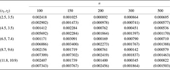


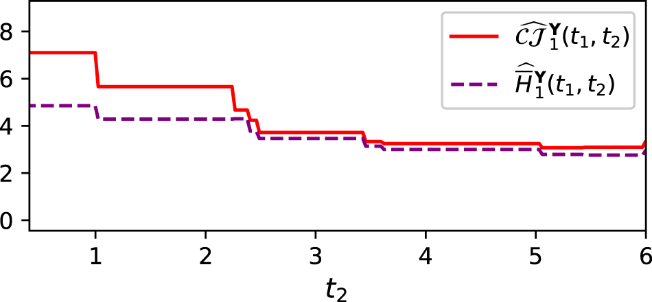

 Open access