







1. Introduction
The wide range of scales involved in turbulent boundary layers and other forms of wall-bounded turbulence, common to many engineering and natural flows, presents a difficult challenge to computational modelling and prediction efforts. The cost of direct numerical simulations (DNS) rises rapidly with increasing Reynolds number, making its use for practical applications computationally infeasible for the foreseeable future. The large-eddy simulation (LES) framework, meanwhile, provides a potential alternative, but wall-resolved LES remains quite costly at high Reynolds numbers (Spalart Reference Spalart2000; Choi & Moin Reference Choi and Moin2012; Yang & Griffin Reference Yang and Griffin2021). Consequently, Reynolds-averaged Navier–Stokes (RANS) models remain relevant and popular. Even with wall-modelled LES or hybrid RANS–LES techniques, scale-resolving simulations can be costly (even prohibitively so) for turbulent boundary layers and immersed bodies at large Reynolds number (Goc, Bose & Moin Reference Goc, Bose and Moin2020).
The RANS-based integral methods for turbulent boundary layers, which pre-date the explosion of computer performance over the past half-century (Kline et al. Reference Kline, Morkovin, Sovran and Cockrell1968), provide a significant reduction in computing cost by seeking a solution for (averaged) quantities integrated in the wall-normal direction across the turbulent boundary layer. For aerodynamic and hydrodynamic boundary layers over immersed bodies, integral methods can be coupled with potential flow solvers to provide rapid prediction, albeit at reduced physical fidelity, e.g. Drela (Reference Drela1989). The use of depth-averaged equations is similarly common in many other wall-bounded turbulence scenarios, e.g. Ungarish (Reference Ungarish2010).
Compared with RANS-based methods, approaches that partially resolve turbulent fluctuations (e.g. LES) potentially offer a substantial advantage in physical fidelity because of their inherent ability to capture non-local behaviour in the large-scale motions. Large-scale motions (LSMs) and very-large-scale motions (VLSMs), sometimes referred to as superstructures, play a prominent role in wall-bounded turbulence. Compared with the turbulent layer thickness (i.e. boundary layer thickness, channel height, pipe radius, etc.), the streamwise lengths of these motions are comparable to and much longer than the turbulent layer thickness and their wall-normal heights are of the order of the turbulent layer thickness (Brown & Thomas Reference Brown and Thomas1977; Monty et al. 2007, 2009; Lee, Sung & Zaki Reference Lee, Sung and Zaki2017). Furthermore, these large streaky structures possess a significant portion of both the Reynolds shear stress and turbulent kinetic energy (Guala, Hommema & Adrian Reference Guala, Hommema and Adrian2006; Balakumar & Adrian Reference Balakumar and Adrian2007). The prominence and significance of these structures raises a motivation for numerical approaches to develop a framework around (V)LSMs. To successfully develop a reduced-order model, it is imperative to encapsulate the essential dynamics of these structures.
The dynamics of streamwise-oriented fluctuations in wall-bounded turbulence received more earlier attention in the context of buffer-layer streaks in the near-wall region (Kline et al. Reference Kline, Reynolds, Schraub and Runstadler1967). It was shown, using DNS on a minimal flow unit, that these turbulent motions of the low-speed structures self-sustain independent of the flow in the outer region (Jiménez & Moin Reference Jiménez and Moin1991; Jiménez & Pinelli Reference Jiménez and Pinelli1999). Further DNS analysis demonstrated the presence of streamwise counter-rotating vortices (Kim, Moin & Moser Reference Kim, Moin and Moser1987). The interplay between streamwise rolls and streaks is crucial for the self-sustaining process of near-wall streaks (Jiménez & Moin Reference Jiménez and Moin1991). Specifically, these rolls produce a ‘lift-up’ effect that generates the observed low-/high-speed streaks. Due to instabilities and/or nonlinear interactions, the streaks become wavy and breakdown. Then, by nonlinear physical mechanisms that result in the breakdown of the streaks, new streamwise vortices are formed to repeat the cycle through another iteration. This is the classical understanding of a self-sustaining process for buffer-layer streaks in the near-wall region (Hamilton, Kim & Waleffe Reference Hamilton, Kim and Waleffe1995).
Adding the log layer and outer region to consideration, the role of the (V)LSMs introduces additional complexities. The fundamental mechanism for producing and sustaining large-scale turbulence has been a topic of significant interest. One possibility is that the (V)LSMs require the interaction with the flow in the inner region. Kim & Adrian (Reference Kim and Adrian1999) hypothesised that a group of hairpin vortices merges to develop the large-scale structures. Studies using particle image velocimetry have made some observations to this effect (Adrian, Meinhart & Tomkins Reference Adrian, Meinhart and Tomkins2000; Jodai & Elsinga Reference Jodai and Elsinga2016), and other DNS studies have also observed merging of the small-scale structures to form larger ones (Toh & Itano 2005; Hwang et al. Reference Hwang, Lee, Sung and Zaki2016). However, significant evidence is now available suggesting that there exists a similar self-sustaining mechanism for LSMs and VLSMs (Cossu & Hwang Reference Cossu and Hwang2017; Lee & Moser Reference Lee and Moser2019; Zhou, Xu & Jiménez Reference Zhou, Xu and Jiménez2022). For example, Hwang & Bengana (Reference Hwang and Bengana2016) observed that the dynamical structure of the large-scale streaks is strikingly similar to that of the near-wall streaks. Even though a wealth of knowledge on (V)LSMs is provided by these and other studies, encapsulating these motions in a reduced-order modelling framework remains a significant opportunity.
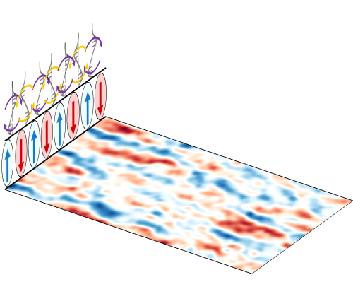
This paper explores the possibility of turbulence-resolving integral simulations (TRIS), that is, LES-like integral methods in which the wall-normal integration is instantaneously carried out across the entire turbulent layer thickness. By reducing the description of the turbulent flow from three to two dimensions, a significant cost savings may be possible while still capturing the physics of (V)LSMs. To the authors’ knowledge, this instantaneous wall-normal integral approach has not been previously proposed or investigated, as it differs substantially from both LES and the common RANS-based integral methods. At the outset, however, it is not clear (i) how much of the turbulence can still be captured in this two-dimensional (2-D) representation, and (ii) how unsteady, 2-D, Navier–Stokes-based evolution equations can be developed which support self-sustaining turbulence with realistic structure. This paper provides an answer for these two questions in the simplified context of an open-channel (half-channel) flow.
The rest of the paper is organised as follows. The governing equations for TRIS are introduced for an open-channel flow configuration in § 2. Then, § 3 estimates the theoretical ability of TRIS to capture a certain fraction of active turbulence using open-channel and full-channel DNS data with $180 \leqslant Re_\tau \leqslant 5200$
. Closure approximations for the TRIS equations are introduced in § 4. Results from their implementation in § 5 demonstrate self-sustaining fluctuations with realistic structure, allowing a detailed apples-to-apples evaluation against open-channel DNS data for
$180 \leqslant Re_\tau \leqslant 5200$
. Closure approximations for the TRIS equations are introduced in § 4. Results from their implementation in § 5 demonstrate self-sustaining fluctuations with realistic structure, allowing a detailed apples-to-apples evaluation against open-channel DNS data for $Re_\tau = 395$
and
$Re_\tau = 395$
and $590$
. A concluding discussion is provided in § 6.
$590$
. A concluding discussion is provided in § 6.
2. Instantaneous moment-of-momentum evolution equations
In this section, evolution equations for TRIS are derived from the Navier–Stokes equations and boundary conditions for an open-channel flow, a useful surrogate with a similar structure to boundary layers. This configuration shares the general characteristics of wall-bounded turbulence while allowing for homogeneity in the wall-parallel direction and simple boundary conditions at the top of the domain (opposite to the no-slip wall). This choice provides a simple starting point for developing the TRIS framework without the added complexities of spatial development and interaction with a potential flow; the details for including these effects in the context of external boundary layer flows are an important topic for future work.
To guide the derivation, the notation will distinguish between wall-normal and wall-parallel components. Using a 2-D index notation, the indices correspond to the streamwise ( $i=1$
) and spanwise (
$i=1$
) and spanwise ( $i=2$
) directions, such that implied summation only applies over the wall-parallel directions. Therefore, the notation used here is
$i=2$
) directions, such that implied summation only applies over the wall-parallel directions. Therefore, the notation used here is $u_1=u$
,
$u_1=u$
, $u_2=w$
and
$u_2=w$
and $v$
along with
$v$
along with $x_1=x$
,
$x_1=x$
, $x_2=z$
and
$x_2=z$
and $y$
for the streamwise, spanwise and wall-normal components of velocity and position, respectively. The conservation equations for incompressible flow are non-dimensionalised by the height of the open channel (
$y$
for the streamwise, spanwise and wall-normal components of velocity and position, respectively. The conservation equations for incompressible flow are non-dimensionalised by the height of the open channel ( $h$
) and friction velocity (
$h$
) and friction velocity ( $u_\tau$
). The bottom wall of the open channel (
$u_\tau$
). The bottom wall of the open channel ( $y=0$
) is a no-slip, no-penetration boundary whereas a no-penetration, zero-vorticity boundary condition is applied at the top wall (
$y=0$
) is a no-slip, no-penetration boundary whereas a no-penetration, zero-vorticity boundary condition is applied at the top wall ( $y=1$
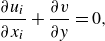
). Using this notation, the incompressible Navier–Stokes equations for conservation of mass, wall-parallel momentum and wall-normal momentum are
$y=1$
). Using this notation, the incompressible Navier–Stokes equations for conservation of mass, wall-parallel momentum and wall-normal momentum are
 \begin{align}&\qquad\qquad\qquad\qquad\qquad \frac {\partial {u_i}}{\partial x_i} + \frac {\partial {v}}{\partial y} = 0, \end{align}
 \begin{align}& \frac {\partial {u_i}}{\partial t} + \frac {\partial {u_i u_j}}{\partial x_j} + \frac {\partial {u_i v}}{\partial y} = -\frac {\partial {p}}{\partial x_i} +\frac {1}{Re_{\tau }}\left ( \frac {\partial ^2 {u_i}}{\partial x_j \partial x_j} + \frac {\partial ^2 {u_i}}{\partial y^2} \right ) + \delta _{i1}, \end{align}
 \begin{align}&\qquad \frac {\partial {v}}{\partial t} + \frac {\partial {v u_j}}{\partial x_j} + \frac {\partial {v v}}{\partial y} = -\frac {\partial {p}}{\partial y} + \frac {1}{Re_{\tau }} \left ( \frac {\partial ^2 {v}}{\partial x_j \partial x_j} + \frac {\partial ^2 {v}}{\partial y^2} \right ). \end{align}
Here, $Re_\tau = \rho u_\tau h / \mu$
is the friction Reynolds number for a fluid with density
$Re_\tau = \rho u_\tau h / \mu$
is the friction Reynolds number for a fluid with density $\rho$
and viscosity
$\rho$
and viscosity $\mu$
. The Kronecker delta,
$\mu$
. The Kronecker delta, $\delta _{i1}$
, is the dimensionless imposed pressure gradient that drives the flow and
$\delta _{i1}$
, is the dimensionless imposed pressure gradient that drives the flow and $p$
is the dimensionless pressure field that enforces (2.1).
$p$
is the dimensionless pressure field that enforces (2.1).
Flow fields are integrated in the wall-normal direction and represented as zeroth and first moments, respectively,
 \begin{equation} \left \langle \phi \right \rangle _0(x_1, x_2, t) = \int _0^1 \phi (x_1, y, x_2, t) {\rm d}y, \qquad \left \langle \phi \right \rangle _1(x_1, x_2, t) = \int _0^1 2y\phi (x_1,y,x_2,t) {\rm d}y. \end{equation}
Thus, the zeroth moment is an unweighted wall-normal integral and the first moment is a wall-normal integral linearly weighted by wall-normal distance to favour events occurring further from the wall. In addition to wall-normal integration, the fields are also low-pass filtered in the wall-parallel directions, $\widetilde {\phi }$
, where the filter width corresponds to the 2-D grid spacing to be used for TRIS.
$\widetilde {\phi }$
, where the filter width corresponds to the 2-D grid spacing to be used for TRIS.
The filtered zeroth and first moments of (2.1) are
 \begin{equation} \frac {\partial \langle \widetilde {u}_i \rangle _0}{\partial x_i} = 0, \qquad \qquad \frac {\partial \langle \widetilde {u}_i \rangle _1}{\partial x_i} = 2 \langle \widetilde {v} \rangle _0, \end{equation}
where the zeroth moment of the wall-parallel velocity, $\langle \widetilde {u}_i \rangle _0$
, is a 2-D, two-component (2D/2C) vector field with zero divergence. The no-penetration condition at the upper boundary has been applied in the first moment of the mass equation. The first moment of the wall-parallel velocity,
$\langle \widetilde {u}_i \rangle _0$
, is a 2-D, two-component (2D/2C) vector field with zero divergence. The no-penetration condition at the upper boundary has been applied in the first moment of the mass equation. The first moment of the wall-parallel velocity, $\langle \widetilde {u}_i \rangle _1$
, is also 2D/2C and has divergence equal to (twice) the zeroth moment of the wall-normal velocity,
$\langle \widetilde {u}_i \rangle _1$
, is also 2D/2C and has divergence equal to (twice) the zeroth moment of the wall-normal velocity, $\langle \widetilde {v} \rangle _0$
. In this way, the inclusion of the first moment provides a three-component (2D/3C) description of the zeroth-moment velocity field.
$\langle \widetilde {v} \rangle _0$
. In this way, the inclusion of the first moment provides a three-component (2D/3C) description of the zeroth-moment velocity field.
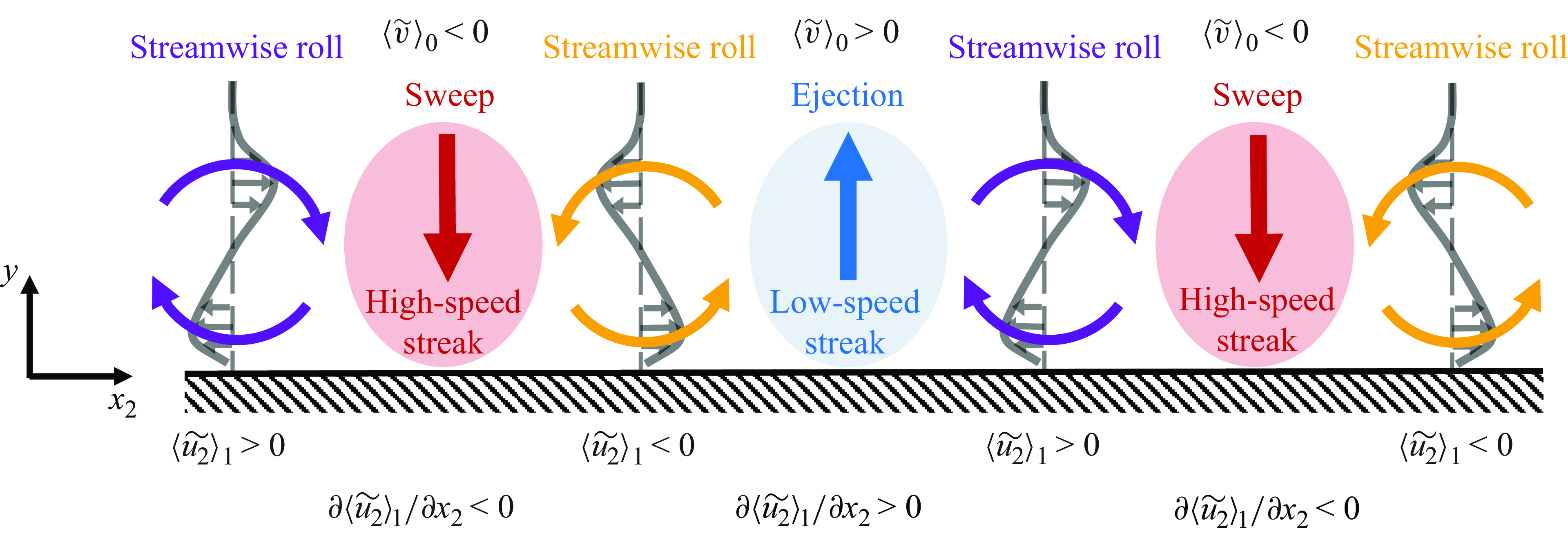
The first moment of mass conservation, (2.5), compactly describes the relationship between streamwise rolls and sweeps/ejections (characterised by $\partial \langle \widetilde {u}_2 \rangle _1 / \partial x_2$
and
$\partial \langle \widetilde {u}_2 \rangle _1 / \partial x_2$
and $\langle \widetilde {v} \rangle _0$
, respectively) that are responsible for the formation of streamwise-oriented streaks. This relationship is illustrated in figure 1, which views a streamwise roll–streak flow pattern in the spanwise-normal plane. In this view, a clockwise roll corresponds to a positive first moment of spanwise velocity,
$\langle \widetilde {v} \rangle _0$
, respectively) that are responsible for the formation of streamwise-oriented streaks. This relationship is illustrated in figure 1, which views a streamwise roll–streak flow pattern in the spanwise-normal plane. In this view, a clockwise roll corresponds to a positive first moment of spanwise velocity, $\langle \widetilde {u}_2 \rangle _1 \gt 0$
, and a counter-clockwise roll corresponds to
$\langle \widetilde {u}_2 \rangle _1 \gt 0$
, and a counter-clockwise roll corresponds to $\langle \widetilde {u}_2 \rangle _1 \lt 0$
. The negative or positive gradients in between two counter-rotating rolls correspond to negative or positive wall-normal velocities, in accordance with (2.5). These sweeps and ejections, respectively, transport fluid across the mean velocity gradient leading to high- and low-speed streaks in between the rolls. Thus, the implementation of (2.5) allows for the proper relationship between streamwise rolls and streaks that participate in the classical picture of the self-sustaining process.
$\langle \widetilde {u}_2 \rangle _1 \lt 0$
. The negative or positive gradients in between two counter-rotating rolls correspond to negative or positive wall-normal velocities, in accordance with (2.5). These sweeps and ejections, respectively, transport fluid across the mean velocity gradient leading to high- and low-speed streaks in between the rolls. Thus, the implementation of (2.5) allows for the proper relationship between streamwise rolls and streaks that participate in the classical picture of the self-sustaining process.
View in the flow direction of the large-scale streamwise rolls generating regions of high- and low-speed streaks, which correspond to sweeps and ejections, respectively. The profiles located at the streamwise rolls represent the local spanwise velocity. This phenomenon encapsulates the effect of (2.5) (right).
The dynamics of the zeroth-moment velocity fields is given by the zeroth moment of (2.2), also including the wall-parallel filtering
 \begin{equation} \frac {\partial \left \langle \widetilde {u}_i \right \rangle _0}{\partial t} + \frac {\partial \langle \widetilde {u_i u_j} \rangle _0}{\partial x_j} = - \frac {\partial \left \langle \widetilde {p} \right \rangle _0}{\partial x_i} + \frac {1}{Re_\tau } \frac {\partial ^2 \left \langle \widetilde {u}_i \right \rangle _0}{\partial x_j \partial x_j} - \widetilde {\tau }_i +\delta _{i1}, \end{equation}
where $\widetilde {\tau }_i$
is the instantaneous (dimensionless) wall shear stress (2D/2C). Equation (2.6) lacks an explicit representation of the turbulent momentum flux in the wall-normal direction. The dynamics of the first-moment velocity field is obtained by applying the first moment to (2.2) along with wall-parallel filtering
$\widetilde {\tau }_i$
is the instantaneous (dimensionless) wall shear stress (2D/2C). Equation (2.6) lacks an explicit representation of the turbulent momentum flux in the wall-normal direction. The dynamics of the first-moment velocity field is obtained by applying the first moment to (2.2) along with wall-parallel filtering
 \begin{equation} \frac {\partial \left \langle \widetilde {u_i} \right \rangle _1}{\partial t} + \frac {\partial \langle \widetilde {u_i u_j} \rangle _1}{\partial x_j} = 2\left \langle \widetilde {u_i v} \right \rangle _0 - \frac {\partial \left \langle \widetilde {p} \right \rangle _1}{\partial x_i} + \frac {1}{Re_\tau } \frac {\partial ^2 \left \langle \widetilde {u_i} \right \rangle _1}{\partial x_j \partial x_j} - \frac {2 \widetilde {u}_{i,\textit{top}}}{Re_\tau } + \delta _{i1}, \end{equation}
where $\widetilde {u}_{i,{top}}$
is the wall-parallel velocity vector (2D/2C) at the top of the open channel (where a Neumann boundary condition is imposed on wall-parallel velocity components and a no-penetration condition is imposed on the wall-normal component). The first moment of the momentum equation includes an explicit representation of turbulent wall-normal momentum flux, namely, the zeroth moment of the Reynolds shear stress,
$\widetilde {u}_{i,{top}}$
is the wall-parallel velocity vector (2D/2C) at the top of the open channel (where a Neumann boundary condition is imposed on wall-parallel velocity components and a no-penetration condition is imposed on the wall-normal component). The first moment of the momentum equation includes an explicit representation of turbulent wall-normal momentum flux, namely, the zeroth moment of the Reynolds shear stress, $\langle \widetilde {u_iv} \rangle _0$
.
$\langle \widetilde {u_iv} \rangle _0$
.
Equations (2.6) and (2.7) contain unclosed terms that need to be modelled: $\widetilde {\tau }_i$
,
$\widetilde {\tau }_i$
, $\langle \widetilde {u_i u_j}\rangle _0$
,
$\langle \widetilde {u_i u_j}\rangle _0$
, $\langle \widetilde {u_i u_j}\rangle _1$
,
$\langle \widetilde {u_i u_j}\rangle _1$
, $\langle \widetilde {u_i v}\rangle _0$
and
$\langle \widetilde {u_i v}\rangle _0$
and $\widetilde {u}_{i,{top}}$
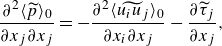
. The divergence of (2.6) and (2.7) provide elliptic equations for the pressure moments,
$\widetilde {u}_{i,{top}}$
. The divergence of (2.6) and (2.7) provide elliptic equations for the pressure moments, $\langle \widetilde {p} \rangle _0$
and
$\langle \widetilde {p} \rangle _0$
and $\langle \widetilde {p} \rangle _1$
 \begin{align}&\qquad\qquad \frac {\partial ^2 \langle \widetilde {p} \rangle _0}{\partial x_j \partial x_j} = - \frac {\partial ^2 \langle \widetilde {u_i u_j} \rangle _0}{\partial x_i \partial x_j} - \frac {\partial \widetilde {\tau }_j}{\partial x_j}, \end{align}
 \begin{align}& \frac {\partial ^2 \langle \widetilde {p} \rangle _1}{\partial x_j \partial x_j} = 2[\widetilde {p}_{{top}} -\widetilde {p}_{{bot}}] - \frac {\partial ^2 \langle \widetilde {u_i u_j} \rangle _1}{\partial x_i \partial x_j} + 4 \frac {\partial \langle \widetilde {u_i v} \rangle _0}{\partial x_i}. \end{align}
The zeroth moment of (2.3) has been used to simplify (2.9). Here, $\widetilde {p}_{{top}}$
and
$\widetilde {p}_{{top}}$
and $\widetilde {p}_{{bot}}$
are the pressures at the top and bottom of the open channel, respectively, and their difference must be modelled to close the system of equations.
$\widetilde {p}_{{bot}}$
are the pressures at the top and bottom of the open channel, respectively, and their difference must be modelled to close the system of equations.
3. Turbulence resolution estimate
Before introducing closure models for (2.6)–(2.9), it is worthwhile to consider how much of the turbulent motions can theoretically be captured in this 2D/3C representation of the flow. This is accomplished by asking a more specific question in terms of the turbulent enhancement of the skin friction coefficient, $C_f = 2 / \overline {u}_{{top}}^2$
, relative to a laminar flow with the same
$C_f = 2 / \overline {u}_{{top}}^2$
, relative to a laminar flow with the same $Re_{{top}} = \overline {u}_{{top}} Re_\tau$
. The
$Re_{{top}} = \overline {u}_{{top}} Re_\tau$
. The $\overline {\phi }$
operator denotes a Reynolds average, and the fluctuation about the mean is
$\overline {\phi }$
operator denotes a Reynolds average, and the fluctuation about the mean is $\phi ^{\prime } = \phi - \overline {\phi }$
.
$\phi ^{\prime } = \phi - \overline {\phi }$
.
Subtracting (2.7) from (2.6) and averaging, assuming statistical stationarity and homogeneity in the wall-parallel directions
 \begin{equation} 1 = 2\frac {\overline {u}_{{top}}}{Re_\tau } + 2\big\langle -\overline {u^\prime v^\prime }\big\rangle _0 = \frac {\frac {4}{Re_{{top}}} + \frac {\big\langle -4\overline {u^\prime v^\prime }\big\rangle _0}{\overline {u}_{{top}}^2}}{C_f} = \frac {C_{f,{lam}} + C_{f,{turb}}}{C_f}, \end{equation}
where $C_{f,{lam}} = 4 Re_{{top}}^{-1}$
is the skin friction coefficient of a laminar open-channel flow, therefore
$C_{f,{lam}} = 4 Re_{{top}}^{-1}$
is the skin friction coefficient of a laminar open-channel flow, therefore $C_{f,{turb}} = - 4 \langle \overline {u^\prime v^\prime }\rangle _0 / \overline {u}_{{top}}^2$
represents the turbulent enhancement of the skin friction coefficient relative to the laminar state. This type of equation was previously introduced as the angular momentum integral (AMI) equation by Elnahhas & Johnson (Reference Elnahhas and Johnson2022) for spatially developing boundary layers. The turbulent enhancement,
$C_{f,{turb}} = - 4 \langle \overline {u^\prime v^\prime }\rangle _0 / \overline {u}_{{top}}^2$
represents the turbulent enhancement of the skin friction coefficient relative to the laminar state. This type of equation was previously introduced as the angular momentum integral (AMI) equation by Elnahhas & Johnson (Reference Elnahhas and Johnson2022) for spatially developing boundary layers. The turbulent enhancement, $C_{f,{turb}}$
, is partially resolved by the 2D/3C zeroth-moment velocity vector field,
$C_{f,{turb}}$
, is partially resolved by the 2D/3C zeroth-moment velocity vector field, $\langle \overline {u^\prime v^\prime }\rangle _0 = \overline {\langle \widetilde {u} \rangle _0^\prime \langle \widetilde {v} \rangle _0^\prime } + \langle \overline {u^{\prime \prime } v^{\prime \prime }}\rangle _0$
, where
$\langle \overline {u^\prime v^\prime }\rangle _0 = \overline {\langle \widetilde {u} \rangle _0^\prime \langle \widetilde {v} \rangle _0^\prime } + \langle \overline {u^{\prime \prime } v^{\prime \prime }}\rangle _0$
, where $\phi ^{\prime \prime } = \phi ^\prime - \langle \widetilde {\phi } \rangle _0^\prime$
is the unresolved portion of a fluctuating field when integrated in the wall-normal direction and filtered in the wall-parallel directions. Thus, the turbulent skin friction enhancement is the sum of a resolved and unresolved portion,
$\phi ^{\prime \prime } = \phi ^\prime - \langle \widetilde {\phi } \rangle _0^\prime$
is the unresolved portion of a fluctuating field when integrated in the wall-normal direction and filtered in the wall-parallel directions. Thus, the turbulent skin friction enhancement is the sum of a resolved and unresolved portion, $C_{f,{turb}} = C_{f,{res}} + C_{f,{unres}}$
.
$C_{f,{turb}} = C_{f,{res}} + C_{f,{unres}}$
.
Note that the skin friction in terms of the velocity at the top of the open-channel domain corresponds more closely to the typical definition for boundary layer flows, whereas friction factors based on the bulk velocity (flow rate) are more common for internal flows such as pipes and channels. The reason for the choice depends on the context. Internal flows are typically analysed in terms of flow rates whereas the potential flow velocity (or edge velocity) is more relevant for boundary layer contexts. Thus, the choice of this $C_f$
definition reflects an interest in analysing the open-channel flow as one would treat the engineering context of an external boundary layer. The alternative choice to analyse the open-channel flow in terms of friction factor based on bulk velocity (flow rate) would lead to the use of the Fukagata–Iwamoto–Kasagi (FIK) equation (Fukagata, Iwamoto & Kasagi Reference Fukagata, Iwamoto and Kasagi2002; Nikora et al. Reference Nikora, Stoesser, Cameron, Stewart, Papadopoulos, Ouro, McSherry, Zampiron, Marusic and Falconer2019; Duan et al. Reference Duan, Zhong, Wang, Zhang and Li2021), which is derived from the second moment of momentum equation and contains the first moment of the Reynolds shear stress. Elnahhas & Johnson (Reference Elnahhas and Johnson2022) discuss the similarities and differences between the AMI and FIK equations in more detail.
$C_f$
definition reflects an interest in analysing the open-channel flow as one would treat the engineering context of an external boundary layer. The alternative choice to analyse the open-channel flow in terms of friction factor based on bulk velocity (flow rate) would lead to the use of the Fukagata–Iwamoto–Kasagi (FIK) equation (Fukagata, Iwamoto & Kasagi Reference Fukagata, Iwamoto and Kasagi2002; Nikora et al. Reference Nikora, Stoesser, Cameron, Stewart, Papadopoulos, Ouro, McSherry, Zampiron, Marusic and Falconer2019; Duan et al. Reference Duan, Zhong, Wang, Zhang and Li2021), which is derived from the second moment of momentum equation and contains the first moment of the Reynolds shear stress. Elnahhas & Johnson (Reference Elnahhas and Johnson2022) discuss the similarities and differences between the AMI and FIK equations in more detail.
Direct numerical simulation was used to compute the terms in the AMI equation, including the resolved and unresolved components of the Reynolds shear stress, for $180 {\leq } Re_\tau {{\leq }} 5200$
on a domain size of
$180 {\leq } Re_\tau {{\leq }} 5200$
on a domain size of $L_x=8\pi$
and
$L_x=8\pi$
and $L_z=3\pi$
. The lower friction Reynolds number flows (
$L_z=3\pi$
. The lower friction Reynolds number flows ( $Re_\tau = 180, 395, 590$
) were simulated using a second-order, staggered finite difference code (Lozano-Durán et al. Reference Lozano-Durán, Hack and Moin2018) for both full-channel and open-channel configurations and the data for the larger Reynolds numbers (
$Re_\tau = 180, 395, 590$
) were simulated using a second-order, staggered finite difference code (Lozano-Durán et al. Reference Lozano-Durán, Hack and Moin2018) for both full-channel and open-channel configurations and the data for the larger Reynolds numbers ( $Re_\tau = 1000, 5200$
) are full-channel simulations from the Johns Hopkins Turbulence Databases (Lee & Moser Reference Lee and Moser2015; Graham et al. Reference Graham2016). Note that (3.1) is equally valid for the bottom half of a full-channel flow where
$Re_\tau = 1000, 5200$
) are full-channel simulations from the Johns Hopkins Turbulence Databases (Lee & Moser Reference Lee and Moser2015; Graham et al. Reference Graham2016). Note that (3.1) is equally valid for the bottom half of a full-channel flow where $\overline {u}_{{top}}$
corresponds to the average centreline velocity and
$\overline {u}_{{top}}$
corresponds to the average centreline velocity and $h$
is the half-height of the full channel. The results using a spectral cutoff filter with
$h$
is the half-height of the full channel. The results using a spectral cutoff filter with $k_{{cut}} h=16$
applied to the streamwise and spanwise directions are shown in figure 2,
$k_{{cut}} h=16$
applied to the streamwise and spanwise directions are shown in figure 2, $k_{cut} = \pi/\delta$
, where
$k_{cut} = \pi/\delta$
, where $\delta$
is the coarsened grid spacing representative of the filtered field. In this analysis, the isotropic cutoff filter of
$\delta$
is the coarsened grid spacing representative of the filtered field. In this analysis, the isotropic cutoff filter of $k_{{cut}}h=16$
is chosen based on the grid resolution used in § 5. Finer wall-parallel resolution does not significantly increase
$k_{{cut}}h=16$
is chosen based on the grid resolution used in § 5. Finer wall-parallel resolution does not significantly increase $C_{f,{res}}$
(Ragan, Warnecke & Johnson Reference Ragan, Warnecke and Johnson2025). The estimated statistical convergence error, following Shirian, Horwitz & Mani (Reference Shirian, Horwitz and Mani2023), is approximately equal to or smaller than the size of the symbols used, and is further discussed in Appendix A. There is no noticeable difference between open-channel and full-channel flow results for friction Reynolds numbers
$C_{f,{res}}$
(Ragan, Warnecke & Johnson Reference Ragan, Warnecke and Johnson2025). The estimated statistical convergence error, following Shirian, Horwitz & Mani (Reference Shirian, Horwitz and Mani2023), is approximately equal to or smaller than the size of the symbols used, and is further discussed in Appendix A. There is no noticeable difference between open-channel and full-channel flow results for friction Reynolds numbers $180$
to
$180$
to $590$
, providing the basis to use full-channel flow datasets at higher Reynolds numbers (
$590$
, providing the basis to use full-channel flow datasets at higher Reynolds numbers ( $1000$
and
$1000$
and $5200$
) to estimate the AMI results for the open-channel configuration.
$5200$
) to estimate the AMI results for the open-channel configuration.
Decomposition of the total skin friction in (3.1). The circular and triangular markers are associated with the authors’ open-channel and full-channel flow simulations, respectively. The star marker corresponds to full-channel flow simulations from previous work (Moser, Kim & Mansour Reference Moser, Kim and Mansour1999; Lee & Moser Reference Lee and Moser2015; Graham et al. Reference Graham2016). The colours black, purple, red and green represent the total, unresolved and resolved skin friction by turbulent enhancement and laminar skin friction, respectively. The purple and red dashed lines are at values of $ {5}/{8}$
and
$ {5}/{8}$
and ${3}/{8}$
, respectively.
${3}/{8}$
, respectively.
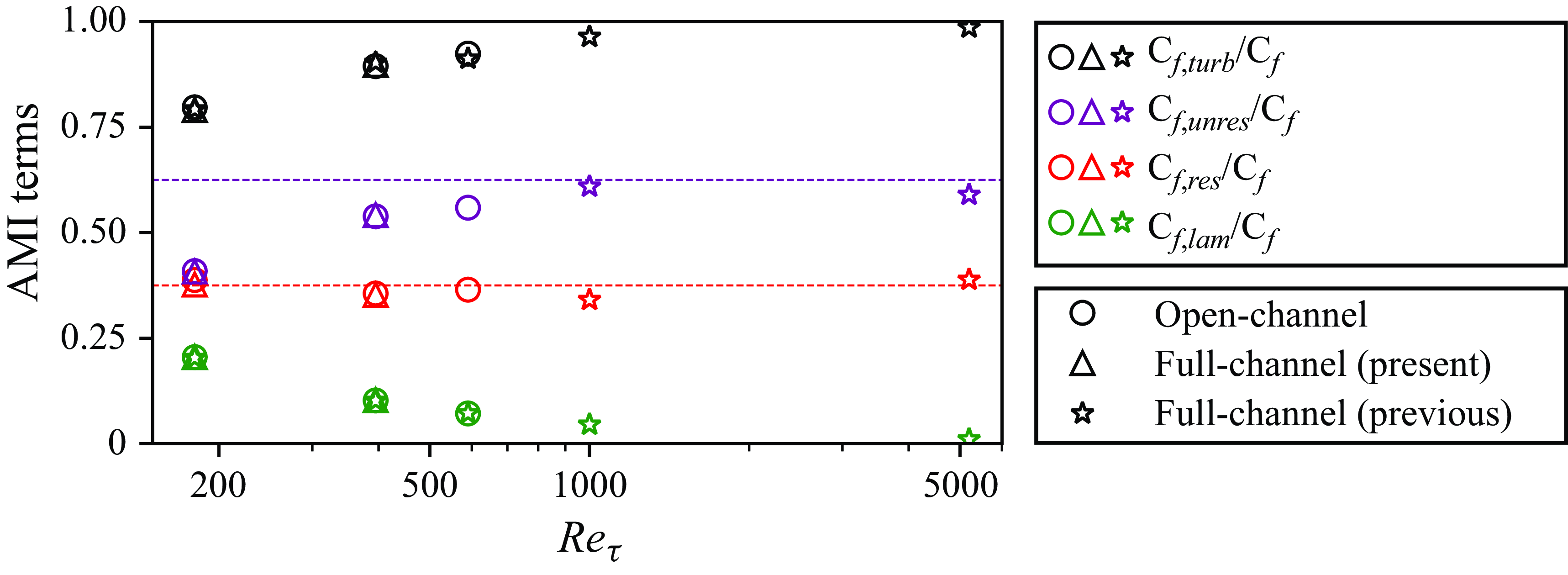
As expected, the laminar skin friction decays with increasing $Re_\tau$
, so the sum of the resolved and unresolved components of the total turbulent enhancement approaches unity. The unresolved portion generally increases with
$Re_\tau$
, so the sum of the resolved and unresolved components of the total turbulent enhancement approaches unity. The unresolved portion generally increases with $Re_\tau$
and appears to approach an asymptotic value based on the available data. Assuming the observed trends continue, it may be estimated that the TRIS equations derived in § 2 can resolve approximately
$Re_\tau$
and appears to approach an asymptotic value based on the available data. Assuming the observed trends continue, it may be estimated that the TRIS equations derived in § 2 can resolve approximately $35\,\%{-}40\, \%$
of the turbulent skin friction enhancement at large Reynolds numbers using a numerical resolution of
$35\,\%{-}40\, \%$
of the turbulent skin friction enhancement at large Reynolds numbers using a numerical resolution of ${\sim}h/5$
in the wall-parallel directions. This theoretical estimate is based on DNS data for open-channel and full-channel flows, and it is not tied to any particular implementation of closure models for TRIS.
${\sim}h/5$
in the wall-parallel directions. This theoretical estimate is based on DNS data for open-channel and full-channel flows, and it is not tied to any particular implementation of closure models for TRIS.
4. Closure approximations
To perform a TRIS calculation, a few unclosed terms in (2.6)–(2.9) need to be approximated in terms of the resolved 2-D fields. The present objective is to demonstrate the sufficiency of the framework presented in § 2 for supporting self-sustaining turbulent fluctuations with realistic structure. To this end, a simple closure is presented by writing the wall-parallel velocity as $\widetilde {u}_i = U_i + U_i^{\prime \prime }$
, where
$\widetilde {u}_i = U_i + U_i^{\prime \prime }$
, where $U_i(x_1, y, x_2, t)$
is interpreted as the mean velocity profile conditioned on the local resolved state defined by
$U_i(x_1, y, x_2, t)$
is interpreted as the mean velocity profile conditioned on the local resolved state defined by $\langle \widetilde {u_i} \rangle _0(x_1, x_2, t)$
and
$\langle \widetilde {u_i} \rangle _0(x_1, x_2, t)$
and $\langle \widetilde {u_i} \rangle _1(x_1, x_2, t)$
. For now, this conditional mean profile is modelled using a skewed Coles profile (Coles Reference Coles1956)
$\langle \widetilde {u_i} \rangle _1(x_1, x_2, t)$
. For now, this conditional mean profile is modelled using a skewed Coles profile (Coles Reference Coles1956)
 \begin{equation} U_i = \left [ \frac {1}{\kappa } \text{ln} y + \left ( \frac {1}{\kappa } \text{ln}Re_{\ast } + B \right ) \right ] e_{i,\ast } + \left [ \frac {2 \Pi }{\kappa } \text{sin}^2\left (\frac {\pi }{2}y\right ) \right ] e_{i,\Pi }, \end{equation}
where $\kappa =0.41$
is the inverse log slope and
$\kappa =0.41$
is the inverse log slope and $B$
is the log vertical intercept, parameters that are pre-set. The local friction Reynolds number is
$B$
is the log vertical intercept, parameters that are pre-set. The local friction Reynolds number is $Re_{\ast }(x_1, x_2, t)$
and
$Re_{\ast }(x_1, x_2, t)$
and $\Pi (x_1, x_2, t)$
is the local wake parameter. The 2-D unit vectors
$\Pi (x_1, x_2, t)$
is the local wake parameter. The 2-D unit vectors $e_{i,\ast }(x_1, x_2, t)$
and
$e_{i,\ast }(x_1, x_2, t)$
and $e_{i,\Pi }(x_1, x_2, t)$
align with the local wall shear stress and wake correction, respectively, allowing for skew in the instantaneous velocity profile. Specific details on the alignments are provided in Appendix B. The local values of
$e_{i,\Pi }(x_1, x_2, t)$
align with the local wall shear stress and wake correction, respectively, allowing for skew in the instantaneous velocity profile. Specific details on the alignments are provided in Appendix B. The local values of $Re_*$
,
$Re_*$
, $\Pi$
,
$\Pi$
, $e_{i,\ast }$
and
$e_{i,\ast }$
and $e_{i,\Pi }$
are uniquely determined at each point in the
$e_{i,\Pi }$
are uniquely determined at each point in the $x_1-x_2$
plane given the local resolved state defined by the zeroth and first moments,
$x_1-x_2$
plane given the local resolved state defined by the zeroth and first moments, $\langle \widetilde {u}_i \rangle _0 = \langle U_i \rangle _0$
and
$\langle \widetilde {u}_i \rangle _0 = \langle U_i \rangle _0$
and $\langle \widetilde {u}_i \rangle _1 = \langle U_i \rangle _1$
, where it is assumed that the integral moments of the fluctuations about the conditionally averaged velocity profiles are neglected.
$\langle \widetilde {u}_i \rangle _1 = \langle U_i \rangle _1$
, where it is assumed that the integral moments of the fluctuations about the conditionally averaged velocity profiles are neglected.
Equation (4.1) is evaluated at $y=1$
to close
$y=1$
to close $\widetilde {u}_{i,\text{top}}$
. The local wall shear stress
$\widetilde {u}_{i,\text{top}}$
. The local wall shear stress $\widetilde {\tau _i}$
is tied to the log portion of the assumed profile in (4.1)
$\widetilde {\tau _i}$
is tied to the log portion of the assumed profile in (4.1)
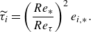 \begin{equation} \widetilde {\tau _i} = \left (\frac {Re_\ast }{Re_\tau }\right )^2 e_{i,\ast }. \end{equation}
The zeroth and first moments of $\widetilde {u_i u_j}$
are closed by decomposing the term into a portion that is resolved by the Coles profile and unresolved (
$\widetilde {u_i u_j}$
are closed by decomposing the term into a portion that is resolved by the Coles profile and unresolved ( $\sigma _{0,ij}$
and
$\sigma _{0,ij}$
and $\sigma _{1,ij}$
)
$\sigma _{1,ij}$
)
 \begin{equation} \langle \widetilde {u_i u_j} \rangle _0 = \langle U_i U_j \rangle _0 + \sigma _{0,ij},\qquad \qquad \langle \widetilde {u_i u_j} \rangle _1 = \langle U_i U_j \rangle _1 + \sigma _{1,ij}. \end{equation}
The resolved portion can be directly computed from the assumed profile, while the unresolved part is modelled by a wall-parallel eddy viscosity approximation (Smagorinsky Reference Smagorinsky1963), $\sigma _{0,ij} = C_s \varDelta ^2 \sqrt {\langle S_{mn} \rangle _{0} \langle S_{mn} \rangle _0} \langle S_{ij} \rangle _{0}$
and
$\sigma _{0,ij} = C_s \varDelta ^2 \sqrt {\langle S_{mn} \rangle _{0} \langle S_{mn} \rangle _0} \langle S_{ij} \rangle _{0}$
and $\sigma _{1,ij} = C_s \varDelta ^2 \sqrt {\langle S_{mn} \rangle _{1} \langle S_{mn} \rangle _1} \langle S_{ij} \rangle _{1}$
, where
$\sigma _{1,ij} = C_s \varDelta ^2 \sqrt {\langle S_{mn} \rangle _{1} \langle S_{mn} \rangle _1} \langle S_{ij} \rangle _{1}$
, where $C_s = 0.78$
is chosen to be a small value that is still large enough to ensure stability,
$C_s = 0.78$
is chosen to be a small value that is still large enough to ensure stability, $S_{ij}$
is the wall-parallel strain rate tensor and
$S_{ij}$
is the wall-parallel strain rate tensor and $\Delta$
is the grid spacing (filter width). The resolved portions,
$\Delta$
is the grid spacing (filter width). The resolved portions, $\langle U_i U_j \rangle _0$
and
$\langle U_i U_j \rangle _0$
and $\langle U_i U_j \rangle _1$
, are linearised about reference (mean) values for the log offset,
$\langle U_i U_j \rangle _1$
, are linearised about reference (mean) values for the log offset, $B$
, and the Coles wake strength,
$B$
, and the Coles wake strength, $\Pi _{{ref}}$
, which are set to match the mean zeroth and first moments of the streamwise velocity computed from DNS.
$\Pi _{{ref}}$
, which are set to match the mean zeroth and first moments of the streamwise velocity computed from DNS.
The $\langle \widetilde {u_i v} \rangle _0$
term is also decomposed into a resolved and unresolved component
$\langle \widetilde {u_i v} \rangle _0$
term is also decomposed into a resolved and unresolved component
 \begin{equation} \left \langle \widetilde {u_i v} \right \rangle _0 = \langle U_i \rangle _0 \langle \widetilde {v} \rangle _0 + \langle \!\widetilde{\,u''_i v''\,}\! \rangle _0. \end{equation}
Here, $\langle \!\widetilde{\,u''_i v''\,}\! \rangle _0$
is modelled using an eddy viscosity with an attached eddy scaling
$\langle \!\widetilde{\,u''_i v''\,}\! \rangle _0$
is modelled using an eddy viscosity with an attached eddy scaling
 \begin{equation} -2\big\langle \!{\widetilde{\,u''_i v''\,}}\! \big\rangle _0 = C_{uv} \frac {\left [1+(1-C_{\Pi })\Pi _{{ref}}\right ]e_{i,\ast } + C_{\Pi }\Pi e_{i,\Pi }}{1 + \Pi _{{ref}}}, \end{equation}
where $C_{uv}$
is set using the AMI balance (the purple symbols in figure 2) and
$C_{uv}$
is set using the AMI balance (the purple symbols in figure 2) and $C_\Pi$
is tuned to allow for the correct amount of resolved Reynolds shear stress,
$C_\Pi$
is tuned to allow for the correct amount of resolved Reynolds shear stress, $\langle U_i \rangle _0 \langle \widetilde {v} \rangle _0$
(the red symbols in figure 2). Lastly, the pressure difference between the top and bottom of the open channel is closed by assuming a linear pressure profile at each location,
$\langle U_i \rangle _0 \langle \widetilde {v} \rangle _0$
(the red symbols in figure 2). Lastly, the pressure difference between the top and bottom of the open channel is closed by assuming a linear pressure profile at each location, $\widetilde {p}_{{top}} - \widetilde {p}_{{bot}} = 6 [\langle \widetilde {p} \rangle _1 - \langle \widetilde {p} \rangle _0 ]$
. A detailed derivation of these closure approximations is available in Appendix B.
$\widetilde {p}_{{top}} - \widetilde {p}_{{bot}} = 6 [\langle \widetilde {p} \rangle _1 - \langle \widetilde {p} \rangle _0 ]$
. A detailed derivation of these closure approximations is available in Appendix B.
5. Results
5.1. Numerical implementation and self-sustaining turbulence
A Python code was developed to solve (2.6)–(2.9) together with the closure models described in § 4 using a pseudo-spectral approach on a doubly periodic domain of size $L_x = 8\pi$
and
$L_x = 8\pi$
and $L_z = 3\pi$
to match the DNS domain. The maximum dimensionless wavenumber is
$L_z = 3\pi$
to match the DNS domain. The maximum dimensionless wavenumber is $k_{{max}} h = k_{{cut}} h = 16$
in the wall-parallel directions, such that the grid spacing based on collocation points is
$k_{{max}} h = k_{{cut}} h = 16$
in the wall-parallel directions, such that the grid spacing based on collocation points is $\varDelta = \pi /16 \approx {1}/{5}$
(five grid points per half-channel thickness). Initially (
$\varDelta = \pi /16 \approx {1}/{5}$
(five grid points per half-channel thickness). Initially ( $t=0$
),
$t=0$
), $\langle \widetilde {u}\rangle _0$
is set to a uniform field based on the approximate mean velocity,
$\langle \widetilde {u}\rangle _0$
is set to a uniform field based on the approximate mean velocity, $\langle \widetilde {u}\rangle _1$
and
$\langle \widetilde {u}\rangle _1$
and $\langle \widetilde {w}\rangle _0$
are initialised to zero, while
$\langle \widetilde {w}\rangle _0$
are initialised to zero, while $\langle \widetilde {w}\rangle _1$
is initialised with white noise. As the simulation advances from the structureless initial conditions, a statistically stationary state emerges with self-sustaining fluctuations. The details of the structure and statistics observed in TRIS simulations are shown below. For now, it is emphasised that the TRIS equations comprising instantaneous zeroth and first-order moments of momentum described in § 2 produce self-sustaining fluctuations when used with the relatively straightforward closures described in § 4. Earlier attempts by the authors to generate self-sustaining turbulence without the first-moment equation were unsuccessful.
$\langle \widetilde {w}\rangle _1$
is initialised with white noise. As the simulation advances from the structureless initial conditions, a statistically stationary state emerges with self-sustaining fluctuations. The details of the structure and statistics observed in TRIS simulations are shown below. For now, it is emphasised that the TRIS equations comprising instantaneous zeroth and first-order moments of momentum described in § 2 produce self-sustaining fluctuations when used with the relatively straightforward closures described in § 4. Earlier attempts by the authors to generate self-sustaining turbulence without the first-moment equation were unsuccessful.
5.2. Choice and verification of model parameters
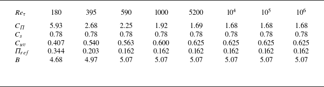
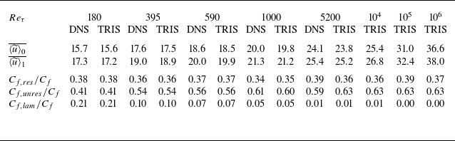
Results in this section are presented for a choice of model parameters shown in table 1. These model parameters are tuned to provide accurate values for the results reported in table 2. Note that the parameter tuning at $Re_\tau = 1000$
and
$Re_\tau = 1000$
and $5200$
relies on full-channel DNS. Results in figure 2 verify that full-channel DNS data provide a good proxy for open-channel flow for the quantities used in the parameter tuning.
$5200$
relies on full-channel DNS. Results in figure 2 verify that full-channel DNS data provide a good proxy for open-channel flow for the quantities used in the parameter tuning.
Values of tuning (and set) parameters in TRIS at various $Re_\tau$
(established in § 4, additional details provided in Appendix B).
$Re_\tau$
(established in § 4, additional details provided in Appendix B).
Verification of TRIS implementation and parameter selection for reproducing target values from DNS.
For Reynolds numbers larger than those with available DNS data, the parameters from $Re_\tau = 5200$
are used. The only exception is that
$Re_\tau = 5200$
are used. The only exception is that $C_\Pi$
is adjusted to close the AMI equation as the viscous term continues to decrease toward zero with increasing
$C_\Pi$
is adjusted to close the AMI equation as the viscous term continues to decrease toward zero with increasing $Re_\tau$
(a very small effect). To verify the successful selection of model parameters according to the above procedure, table 2 shows the target DNS values and the TRIS results. The average zeroth and first moments of streamwise velocity increase with increasing
$Re_\tau$
(a very small effect). To verify the successful selection of model parameters according to the above procedure, table 2 shows the target DNS values and the TRIS results. The average zeroth and first moments of streamwise velocity increase with increasing $Re_\tau$
because the flow variables are normalised by friction velocity and length scales. The statistics in table 2 and the remainder of § 5 are calculated over
$Re_\tau$
because the flow variables are normalised by friction velocity and length scales. The statistics in table 2 and the remainder of § 5 are calculated over $128$
large-eddy turnover times,
$128$
large-eddy turnover times, $h / u_\tau$
.
$h / u_\tau$
.
Importantly, it is demonstrated here that the theoretical resolution of $35\,\%{-}40\, \%$
of the Reynolds shear stress can be achieved with the present TRIS formulation, however simple it may be. Without significant effort to optimise the computational runtime, a flow through time for a domain of length
$35\,\%{-}40\, \%$
of the Reynolds shear stress can be achieved with the present TRIS formulation, however simple it may be. Without significant effort to optimise the computational runtime, a flow through time for a domain of length $L_x = 8\pi$
takes
$L_x = 8\pi$
takes ${\sim}1$
minute on a single processor with a desktop computer. Furthermore, simulations up to
${\sim}1$
minute on a single processor with a desktop computer. Furthermore, simulations up to $Re_\tau =10^6$
were performed without increase in computational cost. Note that these results are for a specific domain size and grid resolution, and that the
$Re_\tau =10^6$
were performed without increase in computational cost. Note that these results are for a specific domain size and grid resolution, and that the $C_\Pi$
coefficient require retuning for different choices of grid spacing and domain size.
$C_\Pi$
coefficient require retuning for different choices of grid spacing and domain size.
Friction factor plotted against the bulk Reynolds number (a) and skin friction plotted against the Reynolds number based on $\overline {u}_{{top}}$
(b). The dashed lines plot full-channel correlations (Dean Reference Dean1978). The grey solid line plots the friction factor correlation for an open-channel flow (Bellos, Nalbantis & Tsakiris Reference Bellos, Nalbantis and Tsakiris2018).
$\overline {u}_{{top}}$
(b). The dashed lines plot full-channel correlations (Dean Reference Dean1978). The grey solid line plots the friction factor correlation for an open-channel flow (Bellos, Nalbantis & Tsakiris Reference Bellos, Nalbantis and Tsakiris2018).
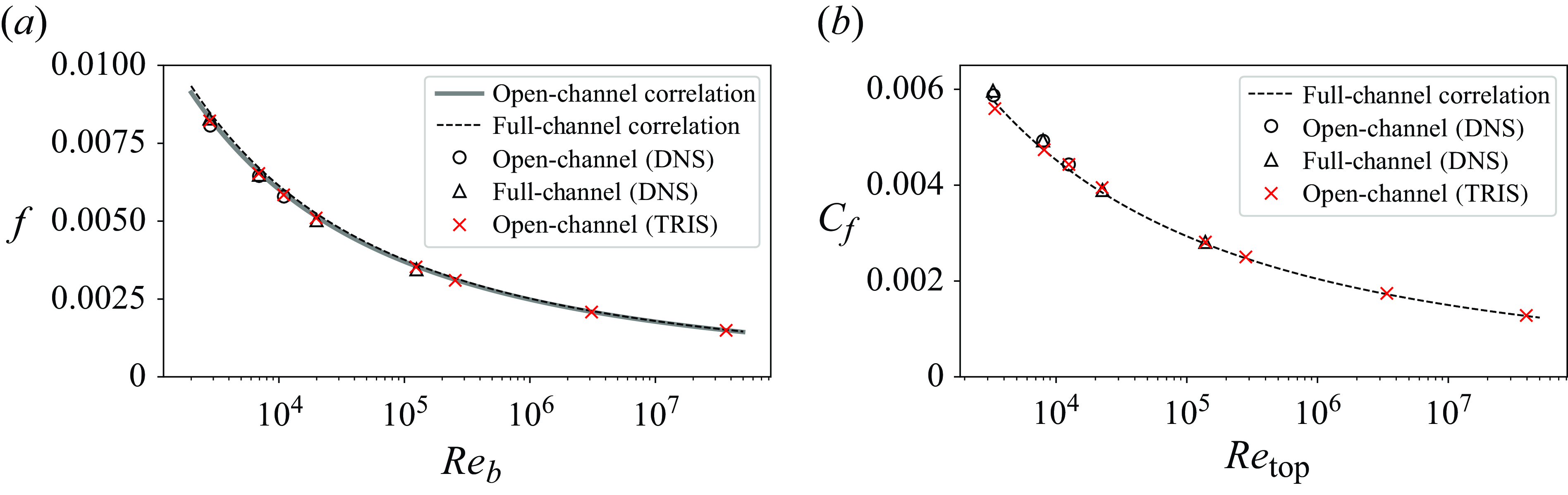
The validity of model parameter extrapolation to high Reynolds number is verified by inspecting TRIS results for the friction factor, $f=2/\langle \overline {u} \rangle _0^2$
, as a function of bulk Reynolds number,
$f=2/\langle \overline {u} \rangle _0^2$
, as a function of bulk Reynolds number, $Re_b=Re_\tau \langle \overline {u}\rangle _0$
, in figure 3. Here, the friction factor is compared with the correlation from Dean (Reference Dean1978) (dashed lines). The successful alignment of TRIS with DNS up to
$Re_b=Re_\tau \langle \overline {u}\rangle _0$
, in figure 3. Here, the friction factor is compared with the correlation from Dean (Reference Dean1978) (dashed lines). The successful alignment of TRIS with DNS up to $Re_\tau = 5200$
and with the empirical correlation at all
$Re_\tau = 5200$
and with the empirical correlation at all $Re_\tau$
demonstrates the success and robustness of the choice of parameters in table 1.
$Re_\tau$
demonstrates the success and robustness of the choice of parameters in table 1.
5.3. Flow structure
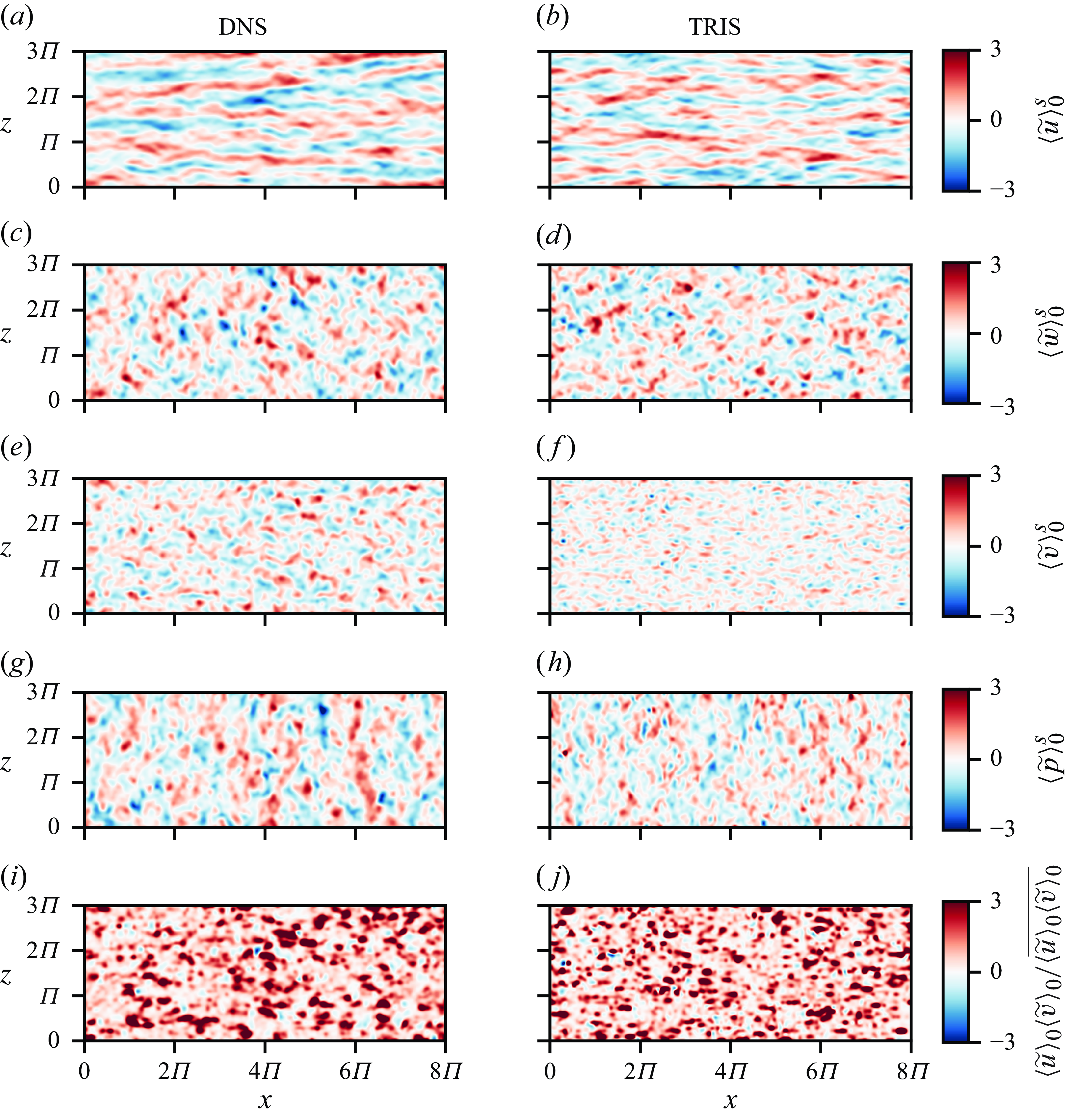
The flow structure in TRIS is now inspected by comparison with the DNS data. For an apples-to-apples comparison, only the open-channel flow DNS data ( $180 \leqslant Re_\tau \leqslant 590$
) are considered in this subsection. First, an instantaneous snapshot from open-channel DNS is integrated in the wall-normal direction and filtered using the spectral cutoff filter corresponding to the TRIS grid resolution. The TRIS simulation reaches a statistically stationary state with streamwise-oriented streaky structures that exhibit the self-sustaining dynamics, as shown in figure 4(a,b). The TRIS results on the right-side column are in comparison with (filtered) zeroth-moment fields from DNS on the left-side column. Results at
$180 \leqslant Re_\tau \leqslant 590$
) are considered in this subsection. First, an instantaneous snapshot from open-channel DNS is integrated in the wall-normal direction and filtered using the spectral cutoff filter corresponding to the TRIS grid resolution. The TRIS simulation reaches a statistically stationary state with streamwise-oriented streaky structures that exhibit the self-sustaining dynamics, as shown in figure 4(a,b). The TRIS results on the right-side column are in comparison with (filtered) zeroth-moment fields from DNS on the left-side column. Results at $Re_\tau = 590$
are visually similar to the
$Re_\tau = 590$
are visually similar to the $Re_\tau = 395$
snapshots shown here.
$Re_\tau = 395$
snapshots shown here.
In order to emphasise flow structure, all fields in figure 4 are standardised (denoted with a superscript $s$
), i.e. fluctuations normalised by their standard deviation. While
$s$
), i.e. fluctuations normalised by their standard deviation. While $\langle \widetilde {u} \rangle _0^s$
(a,b) exhibit relatively realistic streaky structure,
$\langle \widetilde {u} \rangle _0^s$
(a,b) exhibit relatively realistic streaky structure, $\langle \widetilde {w} \rangle _0^s$
and
$\langle \widetilde {w} \rangle _0^s$
and $\langle \widetilde {v} \rangle _0^s$
(c–f, respectively) do not show similar streaks in the TRIS results, in agreement with the flow structure observed from the DNS results. Similarly,
$\langle \widetilde {v} \rangle _0^s$
(c–f, respectively) do not show similar streaks in the TRIS results, in agreement with the flow structure observed from the DNS results. Similarly, $\langle \widetilde {p} \rangle _0^s$
and
$\langle \widetilde {p} \rangle _0^s$
and $\langle \widetilde {u}\rangle _0\langle \widetilde {v}\rangle _0$
(g–j, respectively) do not contain streamwise-oriented streaks. These TRIS results demonstrate that the 2-D-based integral moment equations, derived from the Navier–Stokes equations, are sufficient to generate self-sustaining turbulence with qualitatively realistic structure in a 2D/3C representation.
$\langle \widetilde {u}\rangle _0\langle \widetilde {v}\rangle _0$
(g–j, respectively) do not contain streamwise-oriented streaks. These TRIS results demonstrate that the 2-D-based integral moment equations, derived from the Navier–Stokes equations, are sufficient to generate self-sustaining turbulence with qualitatively realistic structure in a 2D/3C representation.
Instantaneous snapshots of the standardised (denoted by a superscript $s$
)
$s$
) $\langle \widetilde {u}\rangle _0$
,
$\langle \widetilde {u}\rangle _0$
, $\langle \widetilde {w}\rangle _0$
,
$\langle \widetilde {w}\rangle _0$
, $\langle \widetilde {v}\rangle _0$
and
$\langle \widetilde {v}\rangle _0$
and $\langle \widetilde {p}\rangle _0$
fields in descending order at
$\langle \widetilde {p}\rangle _0$
fields in descending order at $Re_\tau = 395$
. The covariance field,
$Re_\tau = 395$
. The covariance field, $\langle \widetilde {u}\rangle _0\langle \widetilde {v}\rangle _0$
, is normalised by its mean. Snapshots are based on the field imposed by a spectral cutoff filter of
$\langle \widetilde {u}\rangle _0\langle \widetilde {v}\rangle _0$
, is normalised by its mean. Snapshots are based on the field imposed by a spectral cutoff filter of $k_{{cut}} h=16$
for DNS (a,c,e,g,i) to match the grid resolution of TRIS (b,d,f,h,j). Videos of the temporal evolution of these fields are available in the supplementary material. For TRIS specifically, a Python code running the time progression of these fields through Jupyter notebook is available at https://www.cambridge.org/S0022112025103248/JFM-Notebooks/files/figure-4.
$k_{{cut}} h=16$
for DNS (a,c,e,g,i) to match the grid resolution of TRIS (b,d,f,h,j). Videos of the temporal evolution of these fields are available in the supplementary material. For TRIS specifically, a Python code running the time progression of these fields through Jupyter notebook is available at https://www.cambridge.org/S0022112025103248/JFM-Notebooks/files/figure-4.
For a quantitative evaluation of the present TRIS formulation (in terms of results that are not set or tuned via closure parameter manipulation), the streamwise and spanwise (co-)spectra of the Reynolds shear stress and three kinetic energy components are shown in figure 5 for $Re_\tau = 395$
and
$Re_\tau = 395$
and $Re_\tau = 590$
. Here,
$Re_\tau = 590$
. Here, $k_i$
is non-dimensionalised by the height of the open channel,
$k_i$
is non-dimensionalised by the height of the open channel, $h$
. Figure 5(a,b) shows the co-spectra for the Reynolds shear stress. The sum of the co-spectra over all streamwise (
$h$
. Figure 5(a,b) shows the co-spectra for the Reynolds shear stress. The sum of the co-spectra over all streamwise ( $k_1 = k_x$
) or spanwise (
$k_1 = k_x$
) or spanwise ( $k_2 = k_z$
) modes is the zeroth moment of the Reynolds shear stress as it shows up in the AMI balance, (3.1), which matches the DNS by means of parameter tuning. More interestingly, the TRIS results show a good degree of success in replicating the shape of the distribution of the Reynolds shear stress as a function of both streamwise (red) and spanwise (blue) wavenumbers. In keeping with the structure observed in figure 4, the co-spectrum peaks at the lowest streamwise wavenumber and at an intermediate spanwise wavenumber. The TRIS results thus reproduce this basic structure, although the spectrum peaks at a larger spanwise wavenumber compared with DNS, which is related to the observation from figure 4 that the typical streak width is generally under-predicted by the current TRIS formulation. The TRIS and DNS results do not show significant sensitivity to
$k_2 = k_z$
) modes is the zeroth moment of the Reynolds shear stress as it shows up in the AMI balance, (3.1), which matches the DNS by means of parameter tuning. More interestingly, the TRIS results show a good degree of success in replicating the shape of the distribution of the Reynolds shear stress as a function of both streamwise (red) and spanwise (blue) wavenumbers. In keeping with the structure observed in figure 4, the co-spectrum peaks at the lowest streamwise wavenumber and at an intermediate spanwise wavenumber. The TRIS results thus reproduce this basic structure, although the spectrum peaks at a larger spanwise wavenumber compared with DNS, which is related to the observation from figure 4 that the typical streak width is generally under-predicted by the current TRIS formulation. The TRIS and DNS results do not show significant sensitivity to $Re_\tau$
.
$Re_\tau$
.
Streamwise (red) and spanwise (blue) spectral distributions of the resolved shear, streamwise, spanwise and wall-normal Reynolds stress components and resolved pressure in descending order at $Re_\tau =395$
(a,c,e,g,i) and
$Re_\tau =395$
(a,c,e,g,i) and $Re_\tau =590$
(b,d,f,h,j). The Fourier transform,
$Re_\tau =590$
(b,d,f,h,j). The Fourier transform, $\widehat {\phi }$
of the resolved component is multiplied by its complex conjugate,
$\widehat {\phi }$
of the resolved component is multiplied by its complex conjugate, $\widehat {\phi }^*$
. The solid and dashed lines represent DNS and TRIS, respectively, and
$\widehat {\phi }^*$
. The solid and dashed lines represent DNS and TRIS, respectively, and $k_i$
is non-dimensionalised by the height of the open channel,
$k_i$
is non-dimensionalised by the height of the open channel, $h$
.
$h$
.
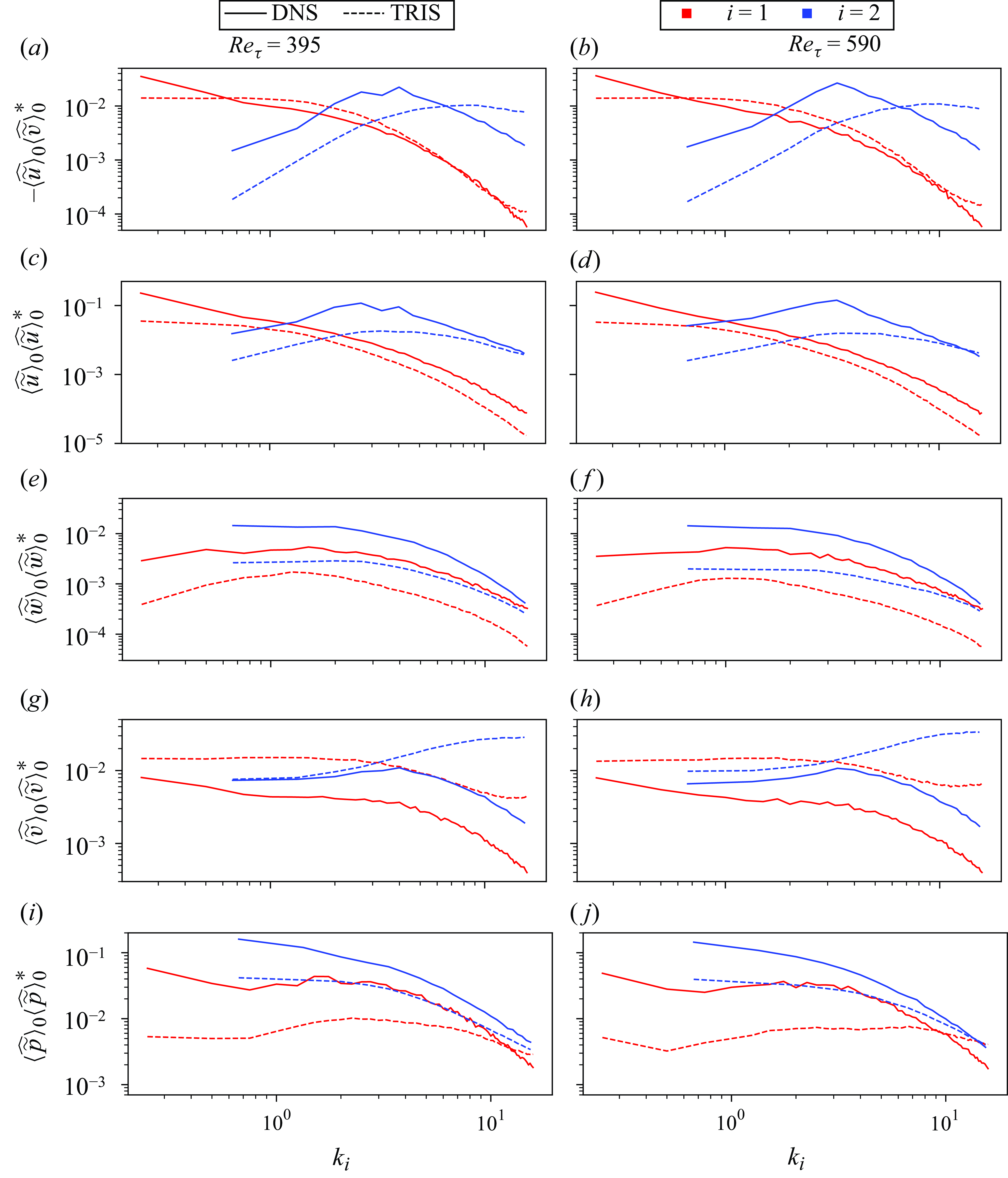
Figure 5(c–h) show the spectra for each of the three components of kinetic energy: Streamwise (c,d), spanwise (e,f), and wall normal (g,h), respectively. The shapes of the spectra of the streamwise and spanwise velocity components produced by the present TRIS formulation are generally similar to the DNS results, but with lower overall magnitude. That is, the root-mean-square of $\langle \widetilde {u} \rangle _0$
and
$\langle \widetilde {u} \rangle _0$
and $\langle \widetilde {w} \rangle _0$
are under-predicted by TRIS. For the wall-normal velocity component, the shape of the TRIS spectra with respect to
$\langle \widetilde {w} \rangle _0$
are under-predicted by TRIS. For the wall-normal velocity component, the shape of the TRIS spectra with respect to $k_1$
is relatively accurate. However, TRIS shows a peak at the highest resolved
$k_1$
is relatively accurate. However, TRIS shows a peak at the highest resolved $k_2$
, which is significantly different than the DNS spectrum. As a result, the
$k_2$
, which is significantly different than the DNS spectrum. As a result, the $\langle \widetilde {v} \rangle _0$
root mean square shows an over-prediction by TRIS. Figure 5(i,j) illustrates the resolved pressure spectra. Here, the TRIS pressure spectra are relatively realistic, although not perfect, with an indication that the magnitude of the large-scale pressure fluctuations are under-predicted.
$\langle \widetilde {v} \rangle _0$
root mean square shows an over-prediction by TRIS. Figure 5(i,j) illustrates the resolved pressure spectra. Here, the TRIS pressure spectra are relatively realistic, although not perfect, with an indication that the magnitude of the large-scale pressure fluctuations are under-predicted.
Two-dimensonal spectral distribution of the resolved Reynolds shear stress, streamwise, spanwise and wall-normal variances, and pressure across panels (a)–(e), respectively. Results are plotted at $Re_\tau =395$
and the Fourier transform,
$Re_\tau =395$
and the Fourier transform, $\widehat {\phi }$
, of the resolved component is multiplied by its complex conjugate,
$\widehat {\phi }$
, of the resolved component is multiplied by its complex conjugate, $\widehat {\phi }^*$
. The dashed black line is a linear line with a slope of unity and a vertical intercept of zero (
$\widehat {\phi }^*$
. The dashed black line is a linear line with a slope of unity and a vertical intercept of zero ( $k_2=k_1$
). In each panel, the spectral fields of DNS and TRIS are on the left and right, respectively. Streamwise (
$k_2=k_1$
). In each panel, the spectral fields of DNS and TRIS are on the left and right, respectively. Streamwise ( $k_1$
) and spanwise (
$k_1$
) and spanwise ( $k_2$
) are non-dimensionalised by the height of the open channel,
$k_2$
) are non-dimensionalised by the height of the open channel, $h$
.
$h$
.
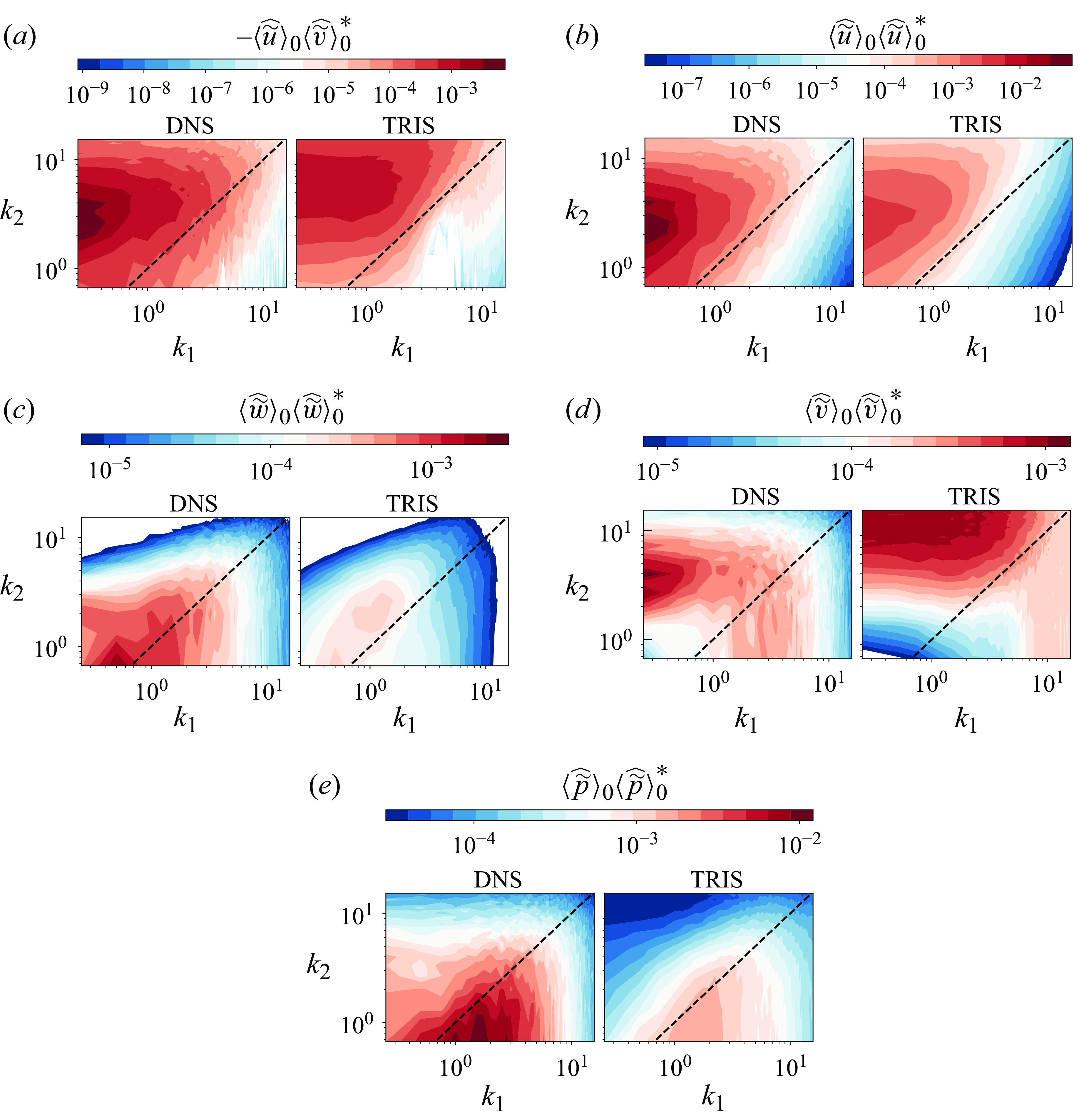
Two-dimensional spectral comparisons between TRIS and DNS at $Re_\tau = 395$
are also illustrated in figure 6, providing a holistic view on the resolved components of the velocity variances/covariances and resolved pressure. The black dashed line,
$Re_\tau = 395$
are also illustrated in figure 6, providing a holistic view on the resolved components of the velocity variances/covariances and resolved pressure. The black dashed line, $k_1 = k_2$
, separates predominantly streamwise-oriented modes (upper left corner) from predominantly spanwise-oriented modes (bottom right corner). Here, TRIS correctly reproduces the relative shape of the u-v co-spectrum with its bias toward streamwise-oriented structures, figure 6(a). It is noted, however, that the co-spectrum maximum is slightly shifted to higher spanwise wavenumber in the TRIS results, in agreement with the 1-D spectra shown above. Also, TRIS generally reproduces the shape of the wall-parallel (streamwise and spanwise) velocity spectra well, figure 6(b,c). The streamwise velocity is dominated by streamwise-oriented modes, while the spanwise velocity is more isotropic. As already observed, the magnitudes of these TRIS spectra are under-predicted. As for the resolved wall-normal variance, the tendency of TRIS to over-predict the most active wavenumbers is again observed. However, the shape of the wall-normal velocity spectrum from TRIS is not altogether unrealistic (although significantly shifted to higher wavenumbers). Lastly, the resolved pressure variance shows that pressure fluctuations occur mostly at low spanwise and intermediate streamwise wavenumbers, corresponding to short and wide structures as illustrated in figure 4(g,h). Also, TRIS presents a similar behaviour, but the overall magnitude is under-predicted, as previously observed.
$k_1 = k_2$
, separates predominantly streamwise-oriented modes (upper left corner) from predominantly spanwise-oriented modes (bottom right corner). Here, TRIS correctly reproduces the relative shape of the u-v co-spectrum with its bias toward streamwise-oriented structures, figure 6(a). It is noted, however, that the co-spectrum maximum is slightly shifted to higher spanwise wavenumber in the TRIS results, in agreement with the 1-D spectra shown above. Also, TRIS generally reproduces the shape of the wall-parallel (streamwise and spanwise) velocity spectra well, figure 6(b,c). The streamwise velocity is dominated by streamwise-oriented modes, while the spanwise velocity is more isotropic. As already observed, the magnitudes of these TRIS spectra are under-predicted. As for the resolved wall-normal variance, the tendency of TRIS to over-predict the most active wavenumbers is again observed. However, the shape of the wall-normal velocity spectrum from TRIS is not altogether unrealistic (although significantly shifted to higher wavenumbers). Lastly, the resolved pressure variance shows that pressure fluctuations occur mostly at low spanwise and intermediate streamwise wavenumbers, corresponding to short and wide structures as illustrated in figure 4(g,h). Also, TRIS presents a similar behaviour, but the overall magnitude is under-predicted, as previously observed.
5.4. Single-point statistics
While the model parameters in table 1 were selected specifically to cause TRIS to provide accurate statistics for the quantities shown in table 2, table 3 shows additional single-point statistics for TRIS and open-channel DNS to further probe the quantitative accuracy of the current TRIS implementation. First, the root-mean-square values for the zeroth moment of the three velocity components and pressure are given. As evidenced in the above spectra, the wall-parallel velocity fluctuation magnitudes are under-predicted while the wall-normal magnitude is over-predicted. This trend is consistent across all wavenumbers for all open-channel flow Reynolds numbers, $180 \leqslant Re_\tau \leqslant 590$
. The under-prediction of the zeroth moment of pressure fluctuation magnitude may be related to the over-prediction of the wall-normal velocity fluctuations. The root-mean-square values for the first moments (not shown) have similar discrepancies between TRIS and DNS.
$180 \leqslant Re_\tau \leqslant 590$
. The under-prediction of the zeroth moment of pressure fluctuation magnitude may be related to the over-prediction of the wall-normal velocity fluctuations. The root-mean-square values for the first moments (not shown) have similar discrepancies between TRIS and DNS.
Additional single-point statistics of TRIS and DNS at various $Re_\tau$
: root-mean-square (
$Re_\tau$
: root-mean-square ( $\text{RMS}\{\phi \}$
), correlation coefficient (
$\text{RMS}\{\phi \}$
), correlation coefficient ( $r(\phi , \psi )$
), skewness (
$r(\phi , \psi )$
), skewness ( $S\{\phi \}$
) and excess kurtosis (
$S\{\phi \}$
) and excess kurtosis ( $K\{\phi \}$
) are listed in descending order. Direct numerical simulation data are available up to
$K\{\phi \}$
) are listed in descending order. Direct numerical simulation data are available up to $Re_\tau =590$
while TRIS data are up to
$Re_\tau =590$
while TRIS data are up to $Re_\tau =10^6$
.
$Re_\tau =10^6$
.
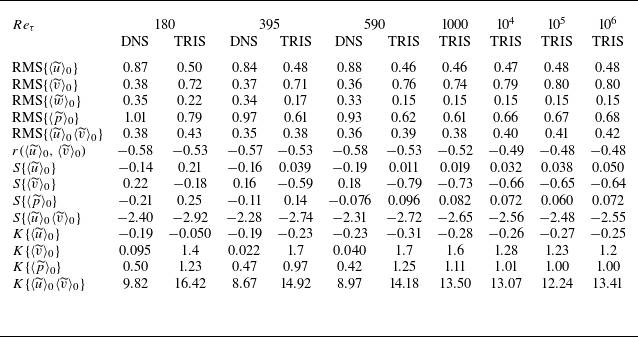
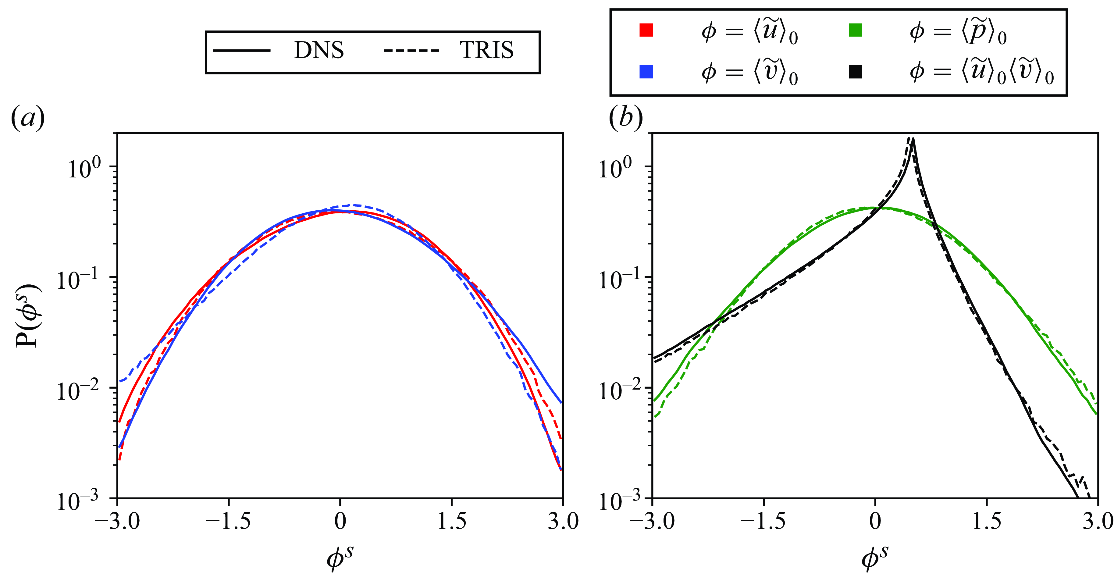
Direct numerical simulation shows that the zeroth moment of the streamwise and wall-normal velocities have slight negative and positive skewness, respectively. (The skewness of the spanwise velocity is zero due to symmetry.) Meanwhile, their excess kurtosis is also close to zero, indicating small departures from Gaussianity. The probability density function (PDF) of each of these velocity components is shown in figure 7(a). The TRIS results, meanwhile, show a very small positive skewness for streamwise velocity and a larger negative skewness and positive excess kurtosis for the wall-normal velocity. Nonetheless, the TRIS PDFs appear relatively close to the Gaussian shape, so the discrepancy with DNS is not strong. The zeroth moment of pressure in DNS has a slight negative skewness and mild positive excess kurtosis. Here, TRIS predicts a slight positive skewness with a larger excess kurtosis. The pressure PDFs are compared in figure 7(b).
The root mean square of the product $\langle \widetilde {u} \rangle _0\langle \widetilde {v} \rangle _0$
is relatively accurate in TRIS, while the negative correlation coefficient of
$\langle \widetilde {u} \rangle _0\langle \widetilde {v} \rangle _0$
is relatively accurate in TRIS, while the negative correlation coefficient of $\langle \widetilde {u} \rangle _0$
and
$\langle \widetilde {u} \rangle _0$
and $\langle \widetilde {v} \rangle _0$
is relatively well represented but under-predicted in magnitude. The PDF of
$\langle \widetilde {v} \rangle _0$
is relatively well represented but under-predicted in magnitude. The PDF of $\langle \widetilde {u} \rangle _0\langle \widetilde {v} \rangle _0$
is shown in figure 7(b). The skewness of
$\langle \widetilde {u} \rangle _0\langle \widetilde {v} \rangle _0$
is shown in figure 7(b). The skewness of $\langle \widetilde {u} \rangle _0\langle \widetilde {v} \rangle _0$
is strongly negative, which TRIS predicts quite well, though TRIS over-predicts its excess kurtosis.
$\langle \widetilde {u} \rangle _0\langle \widetilde {v} \rangle _0$
is strongly negative, which TRIS predicts quite well, though TRIS over-predicts its excess kurtosis.
The statistical results of these higher Reynolds number simulations ( $1000 \leq Re_\tau \leq 10^6$
) are shown in the last four columns of table 3. The root mean squares of
$1000 \leq Re_\tau \leq 10^6$
) are shown in the last four columns of table 3. The root mean squares of $\langle \widetilde {u} \rangle _0$
and
$\langle \widetilde {u} \rangle _0$
and $\langle \widetilde {v} \rangle _0$
display an increasing trend with respect to
$\langle \widetilde {v} \rangle _0$
display an increasing trend with respect to $Re_\tau$
. Beyond
$Re_\tau$
. Beyond $Re_\tau \sim 1000$
, the TRIS predictions show little variation in the single-point statistics as Reynolds number increases.
$Re_\tau \sim 1000$
, the TRIS predictions show little variation in the single-point statistics as Reynolds number increases.
Standardised (denoted with superscript ‘s’) PDFs of the zeroth moments of the streamwise and wall-normal velocity (a) and zeroth moment of pressure and resolved shear stress (b). Solid lines correspond to DNS and the dashed lines correspond to TRIS and comparisons are made for $Re_\tau =395$
.
$Re_\tau =395$
.
6. Concluding discussion
This paper introduces a framework for TRIS of wall-bounded flows. A proof-of-concept demonstration is shown for an open-channel configuration using instantaneous moment-of-momentum integral equations (derived from first principles) with closures based on an assumed profile. The use of zeroth- and first-moment integral equations in a 2-D (streamwise–spanwise) domain provides a sufficient basis for reproducing the self-sustaining process of large-scale streaks in wall-bounded turbulence. The resulting 2D/3C TRIS simulations yield a qualitatively realistic structure for the three velocity components and pressure fields. With a wall-parallel resolution of $h/5$
, DNS evidence suggests that the approach can directly resolve
$h/5$
, DNS evidence suggests that the approach can directly resolve $35\,\%{-} 40\, \%$
of the Reynolds shear stress responsible for turbulent skin friction enhancement. This estimate is relatively constant across a wide range of Reynolds numbers in open-channel and full-channel DNS,
$35\,\%{-} 40\, \%$
of the Reynolds shear stress responsible for turbulent skin friction enhancement. This estimate is relatively constant across a wide range of Reynolds numbers in open-channel and full-channel DNS, $180 \leqslant Re_\tau \leqslant 5200$
, leading the authors to speculate that such resolution will hold for much larger Reynolds numbers. The cost of TRIS is very low compared with established turbulence-resolving techniques such as LES and DNS, with one flow-through time taking
$180 \leqslant Re_\tau \leqslant 5200$
, leading the authors to speculate that such resolution will hold for much larger Reynolds numbers. The cost of TRIS is very low compared with established turbulence-resolving techniques such as LES and DNS, with one flow-through time taking $\sim 1$
minute on a single processor for a channel flow, even at very large Reynolds number, using an unoptimised Python code.
$\sim 1$
minute on a single processor for a channel flow, even at very large Reynolds number, using an unoptimised Python code.
The TRIS framework allows for apples-to-apples quantitative comparisons with DNS data (or experimental data, if available), allowing for a detailed analysis of model accuracy. Overall, the comparisons of spectra and single-point statistics underscore some areas of accuracy for the present TRIS closure model while also highlighting some deficiencies. In particular, the present closures allow for an unrealistically large magnitude of high wavenumber wall-normal velocity fluctuations. The authors speculate that more accurate closure models, e.g. for $\widetilde {p}_{{top}} - \widetilde {p}_{{bot}}$
, could help TRIS produce a more accurate spectra of wall-normal fluctuations with respect to spanwise wavenumber. This could in turn also help yield a more accurate distribution of kinetic energy between the three components. Further work developing physics-based models is deferred to future work.
$\widetilde {p}_{{top}} - \widetilde {p}_{{bot}}$
, could help TRIS produce a more accurate spectra of wall-normal fluctuations with respect to spanwise wavenumber. This could in turn also help yield a more accurate distribution of kinetic energy between the three components. Further work developing physics-based models is deferred to future work.
A related quasi-2D/3C approach to reduced-order modelling of self-sustaining wall-bounded turbulence is the restricted nonlinear model (Thomas et al. Reference Thomas, Lieu, Jovanoviç, Farrell, Ioannou and Gayme2014), which resolves the flow in the spanwise and wall-normal directions while severely restricting the representation of streamwise variations. In comparison, the TRIS approach is well suited for extension to a more general class of flows that are not periodic in the streamwise (or spanwise) direction.
A number of interesting extensions are possible. A multi-layer approach to TRIS could be developed based on performing wall-normal integrals with respect to the inner, log and outer layers, which can potentially capture more physics at the expense of higher computational cost. Of course, identification of the region boundaries and specifying appropriate interface conditions will require detailed study. Analysis by Kwon & Jiménez (Reference Kwon and Jiménez2021) on DNS of an isolated logarithmic region could provide instrumental insight into modelling ideas for this approach. One potentially fruitful topic for future investigation is a more detailed analysis of the production and transport of turbulent kinetic energy from the perspective of instantaneous wall-normal integrals. This could provide more insight into the shortcomings of the present closures and potential pathways for developing closures with higher physical fidelity.
The ability of TRIS to resolve LSMs, which have important sensitivities to favourable and adverse pressure gradients, motivates future development targeting engineering-relevant flows. Future work will aim to formulate the TRIS equations for (external) boundary layer flows. The wall-normal integral of velocity diverges for a semi-infinite domain, so the formulation for boundary layers should be done in terms of velocity defect relative to an irrotational outer flow solution. The AMI equation for boundary layers is formulated this way (Elnahhas & Johnson Reference Elnahhas and Johnson2022). The equations governing the instantaneous zeroth and first moments of the velocity defect can be formulated and the free-stream pressure gradient term would be formally closed. Lacking a no-penetration upper boundary, the boundary layer TRIS formulation will need to account for interaction with an irrotational free-stream flow with zero/non-zero pressure gradients and boundary layer induced fluctuations. Also, the streamwise growth of a boundary layer (i.e. lack of streamwise periodicity) will necessitate the development of realistic inflow boundary conditions, which could be based on recycling–rescaling concepts used in LES and DNS (Lund, Wu & Squires Reference Lund, Wu and Squires1998; Spalart, Strelets & Travin Reference Spalart, Strelets and Travin2006). We have avoided such complications in the present formulation in order to focus on the proof of concept for TRIS itself in terms of the self-sustaining dynamics. The $35\,\%{-}40\, \%$
resolution of the Reynolds shear stress integral by TRIS shown in figure 2 will also need to be reassessed using DNS of spatially developed boundary layers, although the authors expect any changes to be minor.
$35\,\%{-}40\, \%$
resolution of the Reynolds shear stress integral by TRIS shown in figure 2 will also need to be reassessed using DNS of spatially developed boundary layers, although the authors expect any changes to be minor.
Importantly, a truly predictive approach (for engineering quantities of interest) requires more work to establish physics-based closure models to improve the accuracy and general applicability of TRIS compared with the present proof of concept.
Supplementary movies
Supplementary movies and Computational Notebook files are available at https://doi.org/10.1017/jfm.2025.10324. Computational Notebooks can also be found online at https://www.cambridge.org/S0022112025103248/JFM-Notebooks.
Funding
T.R. was supported by the Department of Defense (DoD) National Defense Science & Engineering Graduate (NDSEG) Fellowship Program. M.W. and S.S. were supported by the Air Force Office of Scientific Research under award number FA9550-24-1-0127. P.J. was supported by the National Science Foundation under CAREER award No. 2340121.
Declaration of interests
The authors report no conflict of interest.
Appendix A. Verification and Statistical Convergence of Direct Numerical Simulations
For the lower friction Reynolds number flows ( $Re_\tau = 180, 395, 590$
), the Navier–Stokes equations are solved on a staggered Cartesian grid using a second-order central difference scheme in the wall-parallel directions and an explicit third-order Runge–Kutta scheme for time advancement (Lozano-Durán et al. Reference Lozano-Durán, Hack and Moin2018). Full-channel flow simulations were executed and compared against Moser et al. (Reference Moser, Kim and Mansour1999) to ensure proper spatial discretisation for the open-channel flow application. These lower Reynolds number simulations were run for twenty large-eddy turnover times. For the higher friction Reynolds number flows (
$Re_\tau = 180, 395, 590$
), the Navier–Stokes equations are solved on a staggered Cartesian grid using a second-order central difference scheme in the wall-parallel directions and an explicit third-order Runge–Kutta scheme for time advancement (Lozano-Durán et al. Reference Lozano-Durán, Hack and Moin2018). Full-channel flow simulations were executed and compared against Moser et al. (Reference Moser, Kim and Mansour1999) to ensure proper spatial discretisation for the open-channel flow application. These lower Reynolds number simulations were run for twenty large-eddy turnover times. For the higher friction Reynolds number flows ( $Re_\tau = 1000, 5200$
), velocity data were gathered from the John Hopkins Turbulence Database (Lee & Moser Reference Lee and Moser2015; Graham et al. Reference Graham2016), where the solver uses a Fourier–Galerkin pseudo-spectral method for the wall-parallel directions and a third-order Runge–Kutta scheme for time advancement. These simulations were run for roughly one large-eddy turnover time.
$Re_\tau = 1000, 5200$
), velocity data were gathered from the John Hopkins Turbulence Database (Lee & Moser Reference Lee and Moser2015; Graham et al. Reference Graham2016), where the solver uses a Fourier–Galerkin pseudo-spectral method for the wall-parallel directions and a third-order Runge–Kutta scheme for time advancement. These simulations were run for roughly one large-eddy turnover time.
To ensure the viability of DNS executed by the authors, statistical quantities of the mean velocity and root-mean-square profiles are compared against Moser et al. (Reference Moser, Kim and Mansour1999). Figure 8(a,b) illustrates that the current DNS simulations (at $Re_\tau =180, 395$
) accurately capture mean velocity profiles for the full-channel flow. Here, the grey dashed lines correspond to the fits of the viscous sub-layer and log-layer region. Figure 9(a,b) further shows that, in the full-channel configuration, the root-mean-square statistics sufficiently match with Moser et al. (Reference Moser, Kim and Mansour1999). This analysis demonstrates sufficient spatial discretisation, providing confidence in the accuracy of DNS on the open-channel configuration for
$Re_\tau =180, 395$
) accurately capture mean velocity profiles for the full-channel flow. Here, the grey dashed lines correspond to the fits of the viscous sub-layer and log-layer region. Figure 9(a,b) further shows that, in the full-channel configuration, the root-mean-square statistics sufficiently match with Moser et al. (Reference Moser, Kim and Mansour1999). This analysis demonstrates sufficient spatial discretisation, providing confidence in the accuracy of DNS on the open-channel configuration for $180 \leq Re_\tau \leq 590$
.
$180 \leq Re_\tau \leq 590$
.
Further comparisons of the full-channel and open-channel configurations are illustrated in figure 8(c,d) and 9(c,d). Here, the profile in the full-channel flow extends from the bottom wall (no slip) to the centreline (no boundary condition) whereas the profile in the open-channel flow extends from the bottom wall (no slip) to the top boundary (no vorticity). Interestingly, the mean velocity profiles are statistically identical between these two configurations. However, notable discrepancies are observed in the root-mean-square velocity profiles for $Re_\tau y \gtrsim 125$
, caused by the no-penetration condition at the top boundary. This boundary condition enforces the wall-normal fluctuations to be zero, causing the streamwise and spanwise fluctuations to increase at the top wall.
$Re_\tau y \gtrsim 125$
, caused by the no-penetration condition at the top boundary. This boundary condition enforces the wall-normal fluctuations to be zero, causing the streamwise and spanwise fluctuations to increase at the top wall.
Reynolds-averaged mean velocity profiles of channel flows at $Re_\tau =180$
(a,c) and
$Re_\tau =180$
(a,c) and $Re_\tau =395$
(b,d). The ‘Full-Channel (Previous)’ label (black circular markers) corresponds to the profiles gathered from Moser et al. (Reference Moser, Kim and Mansour1999) whereas the ‘Full-Channel (Present)’ and ‘Open-Channel’ labels (coloured lines and circular markers, respectively) correspond to the author’s DNS data.
$Re_\tau =395$
(b,d). The ‘Full-Channel (Previous)’ label (black circular markers) corresponds to the profiles gathered from Moser et al. (Reference Moser, Kim and Mansour1999) whereas the ‘Full-Channel (Present)’ and ‘Open-Channel’ labels (coloured lines and circular markers, respectively) correspond to the author’s DNS data.
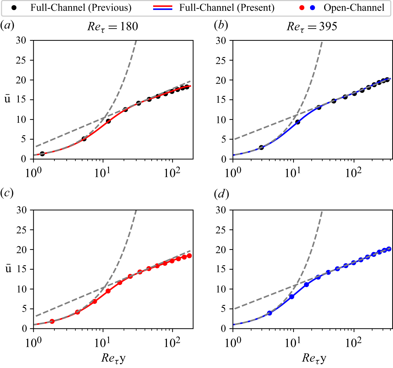
Root-mean-square profiles of channel flows at $Re_\tau =180,395$
(a–d respectively). ‘Full-Channel (Previous)’, denoted by the black circular markers, corresponds to the profiles gathered from Moser et al. (Reference Moser, Kim and Mansour1999) while ‘Full-Channel (Present)’ and ‘Open-Channel’ (denoted by coloured lines and circular markers, respectively) correspond to the author’s DNS data. In all panels, the streamwise, spanwise and wall-normal components are distributed in descending order.
$Re_\tau =180,395$
(a–d respectively). ‘Full-Channel (Previous)’, denoted by the black circular markers, corresponds to the profiles gathered from Moser et al. (Reference Moser, Kim and Mansour1999) while ‘Full-Channel (Present)’ and ‘Open-Channel’ (denoted by coloured lines and circular markers, respectively) correspond to the author’s DNS data. In all panels, the streamwise, spanwise and wall-normal components are distributed in descending order.
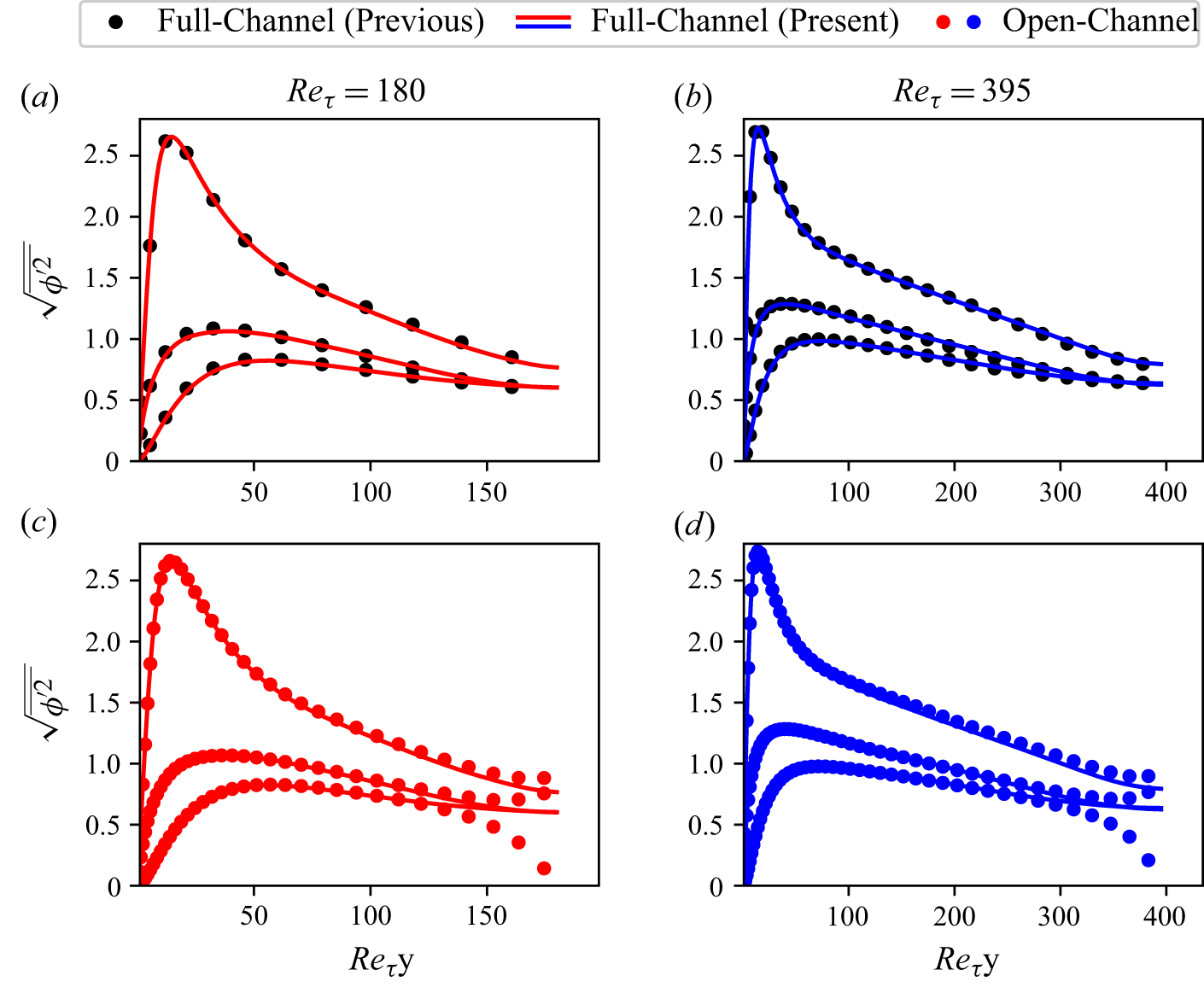
The statistical convergence of the resolved skin friction, $C_{f,{res}}$
, in (3.1) is further analysed. Since LSMs (contributing to
$C_{f,{res}}$
, in (3.1) is further analysed. Since LSMs (contributing to $C_{f,{res}}$
) tend to have longer turnover times than smaller scales (contributing to
$C_{f,{res}}$
) tend to have longer turnover times than smaller scales (contributing to $C_{f,{\textit{unres}}}$
),
$C_{f,{\textit{unres}}}$
), $C_{f,{\textit{unres}}}$
is more statistically converged than its resolved counterpart. As used by Shirian et al. (Reference Shirian, Horwitz and Mani2023), the estimated statistical convergence error (or standard error of the mean) is computed with
$C_{f,{\textit{unres}}}$
is more statistically converged than its resolved counterpart. As used by Shirian et al. (Reference Shirian, Horwitz and Mani2023), the estimated statistical convergence error (or standard error of the mean) is computed with
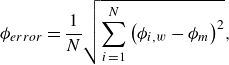 \begin{equation} \phi _{{error}}=\frac {1}{N}\sqrt {\sum _{i=1}^N\left ( \phi _{i,w} - \phi _m \right )^2}, \end{equation}
where $N$
is the number of time windows,
$N$
is the number of time windows, $\phi _{i,w}$
is the average quantity across a particular time window and
$\phi _{i,w}$
is the average quantity across a particular time window and $\phi _m$
is the statistically converged average quantity (Ross Reference Ross1998). According to Shirian et al. (Reference Shirian, Horwitz and Mani2023), estimates of the statistical error can reasonably be computed across
$\phi _m$
is the statistically converged average quantity (Ross Reference Ross1998). According to Shirian et al. (Reference Shirian, Horwitz and Mani2023), estimates of the statistical error can reasonably be computed across $N=4$
windows with a window length of
$N=4$
windows with a window length of $10$
turnover times on a full-channel flow with a domain size of
$10$
turnover times on a full-channel flow with a domain size of $L_x=2\pi$
and
$L_x=2\pi$
and $L_z=1\pi$
. With the present DNS simulations running on a domain size of
$L_z=1\pi$
. With the present DNS simulations running on a domain size of $L_x=8\pi$
and
$L_x=8\pi$
and $L_z=3\pi$
, which is 12 times larger than the previously mentioned domain size, the number of windows and window lengths are modified.
$L_z=3\pi$
, which is 12 times larger than the previously mentioned domain size, the number of windows and window lengths are modified.
For the lower Reynolds number channel flow simulations ( $Re_\tau =180,395,590$
), (A1) of
$Re_\tau =180,395,590$
), (A1) of $C_{f,{res}}$
is computed across
$C_{f,{res}}$
is computed across $N=20$
windows with window lengths of
$N=20$
windows with window lengths of $1$
turnover time. The estimated statistical error of
$1$
turnover time. The estimated statistical error of $C_{f,{res}}$
is less than
$C_{f,{res}}$
is less than $1.0\, \%$
. Alternatively, for the higher Reynolds number simulations (
$1.0\, \%$
. Alternatively, for the higher Reynolds number simulations ( $Re_\tau =1000, 5200$
), the error of
$Re_\tau =1000, 5200$
), the error of $C_{f,{res}}$
is computed across
$C_{f,{res}}$
is computed across $N=2$
windows with window lengths of approximately
$N=2$
windows with window lengths of approximately $1$
turnover time. It turns out that the maximum
$1$
turnover time. It turns out that the maximum $\phi _{{error}}$
value of
$\phi _{{error}}$
value of $C_{f,{res}}$
is approximately
$C_{f,{res}}$
is approximately $2.0\, \%$
.
$2.0\, \%$
.
Higher confidence of the estimated error of the averaged $C_{f,{res}}$
is placed in the lower
$C_{f,{res}}$
is placed in the lower $Re_\tau$
values since more windows are available to compute over. The corresponding estimated values for higher
$Re_\tau$
values since more windows are available to compute over. The corresponding estimated values for higher $Re_\tau$
are (very) rough approximations since more velocity data are required to accurately compute the absolute average (
$Re_\tau$
are (very) rough approximations since more velocity data are required to accurately compute the absolute average ( $\phi _m$
) of the resolved skin friction by turbulent enhancement (i.e. more time windows are required).
$\phi _m$
) of the resolved skin friction by turbulent enhancement (i.e. more time windows are required).
Appendix B. Detailed Derivation of Closure Models for TRIS
For demonstrative purposes, a simple closure is presented by assuming that the skewed Coles wake velocity profile, (4.1),
 \begin{equation} U_i = \left [ \frac {1}{\kappa } \text{ln} y + \left ( \frac {1}{\kappa } \text{ln}Re_{\ast } + B \right ) \right ] e_{i,\ast } + \left [ \frac {2 \Pi }{\kappa } \text{sin}^2\left (\frac {\pi }{2}y\right ) \right ] e_{i,\Pi }, \end{equation}
captures the conditionally averaged wall-parallel profiles ( $U_i(x_1,y, x_2,t) = \langle \widetilde {u_i} | \langle \widetilde {u_i} \rangle _0 , \langle \widetilde {u_i} \rangle _1 \rangle$
). To capture the integral moments, (2.4) is applied to
$U_i(x_1,y, x_2,t) = \langle \widetilde {u_i} | \langle \widetilde {u_i} \rangle _0 , \langle \widetilde {u_i} \rangle _1 \rangle$
). To capture the integral moments, (2.4) is applied to $U_i$
, with the assumption that the moment integrals of the profile fluctuations about the conditional average (
$U_i$
, with the assumption that the moment integrals of the profile fluctuations about the conditional average ( $\langle U_i^{\prime \prime } \rangle _{0}$
and
$\langle U_i^{\prime \prime } \rangle _{0}$
and $\langle U_i^{\prime \prime } \rangle _{1}$
) are negligible,
$\langle U_i^{\prime \prime } \rangle _{1}$
) are negligible,

Applying (2.4) on (4.1) generates the following relations:
 \begin{align}&\qquad\quad \langle U_i \rangle _0 = \left [ \frac {1}{\kappa }\left ( \text{ln}Re_\ast -1 \right ) + B \right ] e_{i,\ast } + \frac {\Pi }{\kappa } e _{i,\Pi }, \end{align}
 \begin{align}& \langle U_i \rangle _1 = \left [ \frac {1}{\kappa }\left ( \text{ln}Re_\ast -\frac {1}{2} \right ) + B \right ] e_{i,\ast } + \frac {\Pi }{\kappa } \left ( 1+\frac {4}{\pi ^2} \right ) e _{i,\Pi }, \end{align}
which are used to solve for $\text{ln}Re_\ast$
,
$\text{ln}Re_\ast$
, $e_{i,\ast }$
,
$e_{i,\ast }$
, $\Pi$
and
$\Pi$
and $e_{i,\Pi }$
. Unit vectors,
$e_{i,\Pi }$
. Unit vectors, $e_{i,\ast }$
and
$e_{i,\ast }$
and $e_{i,\Pi }$
are defined such that
$e_{i,\Pi }$
are defined such that
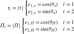 \begin{align} \tau _i = |\tau | \begin{cases} e_{1,\ast } = \text{cos}(\theta _\ast ) & i=1 \\ e_{2,\ast } = \text{sin}(\theta _\ast ) & i=2 \end{cases} \nonumber\\ \Pi _i = |\Pi | \begin{cases} e_{1,\Pi } = \text{cos}(\theta _\Pi ) & i=1 \\ e_{2,\Pi } = \text{sin}(\theta _\Pi ) & i=2 \end{cases} \end{align}
where
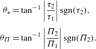 \begin{align} \theta _\ast &= \text{tan}^{-1}\left | \frac {\tau _2}{\tau _1} \right | \text{sgn}(\tau _2), \nonumber \\[4pt] \theta _\Pi &= \text{tan}^{-1}\left | \frac {\Pi _2}{\Pi _1} \right | \text{sgn}(\Pi _2). \end{align}
Note that $\kappa =0.41$
is set for all TRIS simulations. The expressions for these terms are the following:
$\kappa =0.41$
is set for all TRIS simulations. The expressions for these terms are the following:
 \begin{align}& \text{ln} Re_{\ast } = \kappa \left | \left ( \frac {\pi ^2}{4} + 1 \right ) \left \langle \widetilde {u_i} \right \rangle _0 - \frac {\pi ^2}{4} \left \langle \widetilde {u_i} \right \rangle _1 \right | - \kappa B + \frac {\pi ^2}{8} + 1,\\[-10pt]\nonumber \end{align}
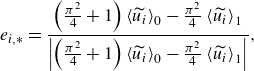 \begin{align}&\qquad\qquad\,\,\, e_{i,\ast } = \frac { \left ( \frac {\pi ^2}{4} + 1 \right ) \left \langle \widetilde {u_i} \right \rangle _0 - \frac {\pi ^2}{4} \left \langle \widetilde {u_i} \right \rangle _1}{\left | \left ( \frac {\pi ^2}{4} + 1 \right ) \left \langle \widetilde {u_i} \right \rangle _0 - \frac {\pi ^2}{4} \left \langle \widetilde {u_i} \right \rangle _1 \right |},\\[-10pt]\nonumber \end{align}
 \begin{align}&\qquad\qquad \Pi = \left |\frac {\pi ^2}{4} \kappa ( \left \langle \widetilde {u_i} \right \rangle _1 - \left \langle \widetilde {u_i} \right \rangle _0) - \frac {\pi ^2}{8} e_{i,\ast } \right |,\\[-10pt]\nonumber \end{align}
 \begin{align}&\qquad\quad e_{i,\Pi } = \frac {1}{\Pi } \left ( \frac {\pi ^2}{4} \kappa ( \left \langle \widetilde {u_i} \right \rangle _1 - \left \langle \widetilde {u_i} \right \rangle _0) - \frac {\pi ^2}{8} e_{i,\ast } \right ). \end{align}
With these formulations, the local values of the shear stress and top velocity are
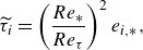 \begin{align}&\qquad\qquad \widetilde {\tau _i} = \left ( \frac {Re_\ast }{Re_{\tau }} \right )^2 e_{i,\ast },\\[-10pt]\nonumber \end{align}
 \begin{align}& U_{T,i} = \left [ \frac {1}{\kappa } \text{ln} Re_{\ast } + B \right ] e_{i,\ast } + \frac {2 \Pi }{\kappa } e_{i,\Pi }, \end{align}
respectively. The pressure is closed by assuming a linear pressure profile that leads to the following relationship between the pressure boundary difference and pressure integral moment difference:
 \begin{equation} \widetilde {p}_{{top}} - \widetilde {p}_{{bot}} = 6 \left [ \langle \widetilde {p} \rangle _1 - \langle \widetilde {p} \rangle _0 \right ]. \end{equation}
For simplicity, the wall-parallel nonlinear terms, $\langle \widetilde {u_i u_j} \rangle _0$
and
$\langle \widetilde {u_i u_j} \rangle _0$
and $\langle \widetilde {u_i u_j} \rangle _1$
, are split into the resolved and unresolved components captured by the Coles profile
$\langle \widetilde {u_i u_j} \rangle _1$
, are split into the resolved and unresolved components captured by the Coles profile
 \begin{equation} \langle \widetilde {u_i u_j} \rangle _0 = \langle U_i U_j \rangle _0 + \sigma _{0,ij},\qquad \qquad \langle \widetilde {u_i u_j} \rangle _1 = \langle U_i U_j \rangle _1 + \sigma _{1,ij}, \end{equation}
where $\sigma _{0,ij}$
and
$\sigma _{0,ij}$
and $\sigma _{1,ij}$
are defined as
$\sigma _{1,ij}$
are defined as
 \begin{equation} \sigma _{0,ij} = C_s \varDelta ^2 \sqrt {\langle S_{mn} \rangle _{0} \langle S_{mn} \rangle _0} \langle S_{ij} \rangle _{0},\qquad \quad \sigma _{1,ij} = C_s \varDelta ^2 \sqrt {\langle S_{mn} \rangle _{1} \langle S_{mn} \rangle _1} \langle S_{ij} \rangle _{1}. \end{equation}
Here, $S_{ij}$
is the strain rate tensor in the wall-parallel directions,
$S_{ij}$
is the strain rate tensor in the wall-parallel directions, $\varDelta$
is the grid spacing of the TRIS simulation and
$\varDelta$
is the grid spacing of the TRIS simulation and $C_s=0.78$
is set for the eddy viscosity coefficient. The conditional (resolved) components are quasi-linearised for robustness, defined as
$C_s=0.78$
is set for the eddy viscosity coefficient. The conditional (resolved) components are quasi-linearised for robustness, defined as
 \begin{align}& \langle U_i U_j \rangle _0 = A_0 (e_{i,\ast } e_{j,\ast }) + B_0 (e_{i,\ast } e_{j,\ast } + e_{i,\Pi } e_{j,\Pi }) + D_0 (e_{i,\Pi } e_{j,\Pi }), \end{align}
 \begin{align}& \langle U_i U_j \rangle _1 = A_1 (e_{i,\ast } e_{j,\ast }) + B_1 (e_{i,\ast } e_{j,\ast } + e_{i,\Pi } e_{j,\Pi }) + D_1 (e_{i,\Pi } e_{j,\Pi }), \end{align}
where
 \begin{align}&\qquad\qquad\qquad\qquad\quad A_0 = \left (2 T_{{ref}} - \frac {2}{\kappa } \right ) T + \left ( \frac {2}{\kappa ^2} - T_{{ref}}^2 \right ),\\[-10pt]\nonumber \end{align}
 \begin{align}&\qquad\qquad\qquad B_0 = \frac {\Pi }{\kappa } T_{{ref}} + \frac {\Pi _{{ref}}}{\kappa } (T - T_{{ref}}) - \frac {\Pi }{\kappa ^2}\left (1 - \frac {\text{Si}(\pi )}{\pi } \right ),\\[-10pt]\nonumber \end{align}
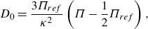 \begin{align}&\qquad\qquad\qquad\qquad\qquad\quad D_0 = \frac {3 \Pi _{{ref}}}{\kappa ^2} \left ( \Pi - \frac {1}{2} \Pi _{{ref}} \right ),\\[-10pt]\nonumber \end{align}
 \begin{align}&\qquad\qquad\qquad\qquad\,\,\, A_1 = \left ( 2 T_{{ref}} - \frac {1}{\kappa } \right ) T + \left ( \frac {1}{2 \kappa ^2} - T_{{ref}}^2 \right ),\\[-10pt]\nonumber \end{align}
 \begin{align}& B_1 = \left (1+ \frac {4}{\pi ^2} \right ) \left (\frac {\Pi }{\kappa }T_{{ref}} \right ) + \frac {\Pi _{{ref}}}{\kappa }(T - T_{{ref}}) - \frac {2\Pi }{\kappa ^2} \left ( \frac {1}{4} - \frac {2 + \text{Cin}(\pi )}{\pi ^2} \right ),\\[-10pt]\nonumber \end{align}
 \begin{align}&\qquad\qquad\qquad\qquad\,\,\,\, D_1 = \left (3+\frac {16}{\pi }\right )\frac {\Pi _{{ref}}}{\kappa ^2}\left (\Pi - \frac {1}{2}\Pi _{{ref}} \right ). \end{align}
From these equations, $T = {1}/{\kappa } \text{ln}Re_{\ast } +B$
and the trigonometric integrals (Abramowitz & Stegun Reference Abramowitz and Stegun1964) are defined as
$T = {1}/{\kappa } \text{ln}Re_{\ast } +B$
and the trigonometric integrals (Abramowitz & Stegun Reference Abramowitz and Stegun1964) are defined as
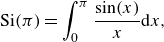 \begin{align}&\quad \text{Si}(\pi )=\int _0^\pi \frac {\text{sin}(x)}{x}{\rm d}x,\\[-10pt]\nonumber \end{align}
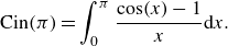 \begin{align}& \text{Cin}(\pi )=\int _0^\pi \frac {\text{cos}(x)-1}{x}{\rm d}x. \end{align}
Here, $T_{{ref}} = ({1}/{\kappa }) \text{ln}Re_{\tau } +B$
and
$T_{{ref}} = ({1}/{\kappa }) \text{ln}Re_{\tau } +B$
and $\Pi _{{ref}}$
are the values at the reference condition. Specifically,
$\Pi _{{ref}}$
are the values at the reference condition. Specifically, $\Pi _{{ref}}$
and
$\Pi _{{ref}}$
and $B$
are set parameters matching the mean values of the streamwise velocity moments from DNS (
$B$
are set parameters matching the mean values of the streamwise velocity moments from DNS ( $\langle \widetilde {u} \rangle _{0,\textit{ref}}$
and
$\langle \widetilde {u} \rangle _{0,\textit{ref}}$
and $\langle \widetilde {u} \rangle _{1,\textit{ref}}$
), values listed in table 3
$\langle \widetilde {u} \rangle _{1,\textit{ref}}$
), values listed in table 3
 \begin{align}&\qquad\qquad\quad\,\, \Pi _{\textit{ref}}=\frac {\pi ^2}{4}\kappa \left ( \overline {\langle \widetilde {u} \rangle }_{1,\textit{ref}} - \overline {\langle \widetilde {u} \rangle }_{0,\textit{ref}} \right ) -\frac {\pi ^2}{8},\\[-10pt]\nonumber \end{align}
 \begin{align}& B=\left (\frac {\pi ^2}{4}+1\right )\overline {\langle \widetilde {u} \rangle }_{0,\textit{ref}} -\frac {\pi ^2}{4}\overline {\langle \widetilde {u} \rangle }_{1,\textit{ref}} +\frac {1}{\kappa }\left [ \frac {\pi ^2}{8} + 1 - \text{ln} Re_\tau \right ]. \end{align}
The $\langle \widetilde {u_i v} \rangle _0$
term is closed by splitting the resolved and unresolved components, as done in § 3
$\langle \widetilde {u_i v} \rangle _0$
term is closed by splitting the resolved and unresolved components, as done in § 3
 \begin{equation} \left\langle \widetilde {u_i v} \right\rangle _0 = \left\langle \widetilde {u_i} \right\rangle _0 \left\langle \widetilde {v} \right\rangle _0 + \big\langle \!\widetilde{\,u''_i v''\,}\! \big\rangle _0, \end{equation}
where $\langle \widetilde {u_i} \rangle _0=\langle U_i \rangle _0$
is known from (B3) and
$\langle \widetilde {u_i} \rangle _0=\langle U_i \rangle _0$
is known from (B3) and $\langle \widetilde {v} \rangle _0$
is known from the right equation in (2.5). The unresolved term,
$\langle \widetilde {v} \rangle _0$
is known from the right equation in (2.5). The unresolved term, $\langle \widetilde {u''_i v''} \rangle _0$
, is closed with an eddy viscosity approximation (with wall-normal scaling) superimposed with effects by the wake
$\langle \widetilde {u''_i v''} \rangle _0$
, is closed with an eddy viscosity approximation (with wall-normal scaling) superimposed with effects by the wake
 \begin{equation} -\big\langle \!\widetilde {\,u_i'' v''\,}\! \big\rangle _0 \approx \int _0^1 \nu _{T,y} \frac {\partial U_i}{\partial y} {\rm d}y + C_T \left ( C_\Pi - 1 \right )\left [ \Pi e_{i,\Pi } - \Pi _{{ref}} e_{i,\ast } \right ] ,\end{equation}
where $\nu _{T,y}$
is an effective (dimensionless) wall-normal turbulent eddy viscosity, which is taken to be
$\nu _{T,y}$
is an effective (dimensionless) wall-normal turbulent eddy viscosity, which is taken to be $\nu _{T,y} \approx C_T \kappa y$
. Here,
$\nu _{T,y} \approx C_T \kappa y$
. Here, $C_T$
is a value that is soon to be defined and
$C_T$
is a value that is soon to be defined and $C_\Pi$
is the tuning coefficient that controls the value of the resolved Reynolds shear stress. Using the skewed Coles profile, (B29) becomes the following:
$C_\Pi$
is the tuning coefficient that controls the value of the resolved Reynolds shear stress. Using the skewed Coles profile, (B29) becomes the following:
 \begin{equation} -2\big\langle \!\widetilde {\,u_i''v''\,}\! \big\rangle _0 \approx C_T\left [1+(1-C_\Pi )\Pi _{{ref}}\right ] e_{i,\ast } +C_T\left [C_\Pi \Pi \right ] e_{i,\Pi }. \end{equation}
At equilibrium ( $\Pi =\Pi _{{ref}}$
and
$\Pi =\Pi _{{ref}}$
and $e_{i,\ast }=e_{i,\Pi }$
)
$e_{i,\ast }=e_{i,\Pi }$
)
 \begin{equation} -2\big\langle \widetilde {\,u_i''v''\,}\! \big\rangle _0 =C_{uv}\delta _{i1} =C_T(1+\Pi _{{ref}})\delta _{i1}, \end{equation}
where $C_{uv}$
is a set parameter to control the amount of unresolved skin friction by turbulent enhancement. As a result,
$C_{uv}$
is a set parameter to control the amount of unresolved skin friction by turbulent enhancement. As a result, $C_T=C_{uv}/(1+\Pi _{{ref}})$
. Therefore, the modelled unresolved Reynolds shear stress is defined as
$C_T=C_{uv}/(1+\Pi _{{ref}})$
. Therefore, the modelled unresolved Reynolds shear stress is defined as
 \begin{equation} -2\big\langle \!\widetilde {\,u''_i v''\,}\! \big\rangle _0 \approx C_{uv} \frac {\left [1+(1-C_{\Pi })\Pi _{{ref}}\right ]e_{i,\ast } + C_{\Pi }\Pi e_{i,\Pi }}{1 + \Pi _{{ref}}}. \end{equation}


 Open access

