1. Introduction

A resurgence of interest in subglacial hydrology, particularly in the Antarctic ice sheet system, has been sparked by the recent successes of satellite altimetry and interferometric synthetic aperture radar (SAR) in detecting subtle localized elevation changes. These are interpreted as active, volume-changing subglacial lakes interconnected by drainage systems (Rémy and Legrésy, 2004; Reference Gray, Joughin, Tulaczyk, Spikes, Bindschadler and JezekGray and others, 2005; Reference Wingham, Siegert, Shepherd and MuirWingham and others, 2006; Reference Fricker, Scambos, Bindschadler and PadmanFricker and others, 2007; Reference Stearns, Smith and HamiltonStearns and others, 2008; Reference Fricker and ScambosFricker and Scambos, 2009). Hundreds of these active subglacial systems have now been identified (Reference Smith, Fricker, Joughin and TulaczykSmith and others, 2009) and, in one case at least, they are shown to affect ice flow (Byrd Glacier; Reference Stearns, Smith and HamiltonStearns and others, 2008). Moreover, compilations of both radar reflection evidence and surface morphological indicators of larger subglacial water bodies (Reference Siegert, Carter, Tabacco, Popov and BlankenshipSiegert and others, 2005; Reference Smith, Fricker, Joughin and TulaczykSmith and others, 2009) show that not only are these also widespread but that they, too, can have important effects on ice flow (e.g. Reference Bell, Studinger, Shuman, Fahnestock and JoughinBell and others, 2007).

Despite these advances, a class of subglacial water bodies remains largely unmapped: smaller pockets (less than a few ice thicknesses across) that remain stable. Since these features may not have a surface elevation change over time associated with them (which permits detection) and do not affect surface morphology significantly, they are detectable only by radio-echo surveys. These surveys are sparsely distributed. In the case of heavily crevassed outlet glaciers, it may be difficult to detect the subglacial water body even with radio-echo surveys. Recent modeling studies of subglacial melt rates (Reference PattynPattyn, 2010) and the irregularity of both surface topography and bed elevation where they are mapped in detail (e.g. West Antarctica (Reference Shabtaie and BentleyShabtaie and Bentley, 1988; http://www.ig.utexas.edu/research/projects/agasea); East Antarctica (Reference BoBo and others, 2009; http://www.ldeo.columbia.edu/~mstuding/AGAP/AGAP_GAM-BIT_maps.html)) show that abundant sub-ice water is available and that there are numerous places where it may be trapped. As our ability to map the base of the ice sheet and detect the presence of subglacial water bodies improves, it is likely that we will find an ice-sheet bed surface as pocked with lakes as the current land areas that were formerly beneath ice sheets (e.g. the Canadian Shield and Scandinavia; Reference ClarkeClarke, 2005).

These small stable water bodies, if widespread, represent an important potential contributor to mass-balance changes as a glacier responds to climate-driven changes in flow. In the case of retreating tidewater glaciers, as glacier mass imbalance increases, the surface slope generally increases as well. Changes in surface slope across a subglacial body of water must create subglacial pressure gradient changes, forcing the confined water to move in the downslope direction. The trapping mechanism that sustained the lake (bedrock sill, sediment plug or a local high in subglacial hydraulic potential) is tested, and if pressure changes are great enough it is breached. The water then drains into the subglacial environment downstream.

At Crane Glacier, an outlet glacier draining the eastern Antarctic Peninsula, we have mapped a case where such an ice-dynamics-driven (more broadly, climate-driven) slope change has apparently caused a subglacial water pocket to drain into the subglacial environment (Fig. 1). Crane Glacier is the largest of the outlet glaciers flowing into the embayment created by the loss of the Larsen B ice shelf in February–March 2002 (Reference Scambos, Bohlander, Shuman and SkvarcaScambos and others, 2004). Response of the several glaciers affected by the shelf loss was almost immediate. There was an acceleration in flow speed, with ice-front flow rates rising to six to eight times the pre-shelf-loss speed by late 2003 (Reference Rignot, Casassa, Gogineni, Krabill, Rivera and ThomasRignot and others, 2004; Reference Scambos, Bohlander, Shuman and SkvarcaScambos and others, 2004), rapid loss of the remaining floating tongues, and widespread new extensional crevassing. However, by early 2004, Crane Glacier had slowed significantly, to just twice the pre-break-up speed, before re-accelerating in 2005 (Reference Hulbe, Scambos, Youngberg and LambHulbe and others, 2008). Shuman and others (in press) discuss the regional elevation changes and mass-balance response since shelf break-up.

Fig. 1. Satellite image map of lower Crane Glacier and fjord. Inset: locator map of Crane Glacier, within the Larsen B embayment, Antarctic Peninsula; dates and extent of major ice-shelf break-up events for the region are shown. Main image is from SPOT-5 high-resolution stereo (HRS) sensor, acquired 25 November 2006. Recent airborne laser altimetry tracks (ATM: 2002, 2004 and 2008 in yellow, orange and red respectively) and satellite laser altimetry tracks (ICESat: 2003–09, straight green line) show significant elevation changes on the glacier, which are anomalously large in the irregular region at their intersection (interpreted in this study as resulting from a subglacial lake). Bathymetric contours of the fjord are from multi-beam sonar mapping in 2006 (personal communication from E. Domack, 2011). Numbers in the fjord (1, 2 and 3) and dashed outlines represent flat sediment-filled basins interpreted as past subglacial lake deposits. Grounding line of 1998–2002 is from SAR interferometry (Reference Rack and RottRack and Rott, 2004). Ice-front locations for floating (November 2002) and grounded ice fronts are shown; since November 2006 the ice-front position has been essentially unchanged.

In the following, we compile evidence from satellite and airborne laser altimetry, satellite stereo-image digital elevation models (DEMs) and image pair velocity maps that examine the period of renewed rapid changes on Crane in 2004, 2005 and 2006, concluding that some of this change was the result of subglacial lake drainage. However, retreat of the glacier front from a bedrock high in the Crane fjord, as mapped by bathymetry (Reference MuellerMueller and others 2006, fig. 1; personal communication from E. Domack, 2011), also played a role in the glacier evolution at the time of the inferred lake drainage. We compare the significance of the lake drainage and ice-front retreat on elevation change, ice flow and mass balance for Crane Glacier, and thereby gain some insight into the importance of a potential subglacial water feedback on retreating outlet glaciers.

2. Data Sources and Methods

2.3. Satellite stereo-image digital elevation models and DEM differencing

We also generated a series of DEMs of the Crane Glacier trunk and nearby glaciers, from satellite stereo digital images (Table 1).We used six such stereo-image DEMs in evaluating the topographic evolution of lower Crane Glacier. The two sensors used are the Advanced Spaceborne Thermal Emission and Reflection Radiometer (ASTER) flying on NASA’s Terra platform, and SPOT-5, the fifth satellite of the Système Probatoire pour l’Observation de la Terre (SPOT) series. Both these satellites acquire along-track stereo imagery by a fore and aft (or nadir and aft) acquisition scheme. The systems have imagery with 15 and 5 m resolution, respectively, and under ideal conditions can resolve elevations to ~5m (Reference Fujisada, Bailey, Kelly, Hara and AbramsFujisada and others, 2005; Reference Bouillon, Bernard, Gigord, Orsoni, Rudowski and BaudoinBouillon and others, 2006; Reference ToutinToutin, 2008). However, problems with sky clarity, snow/ice reflectance variations and extreme surface roughness at the pixel scale can reduce this accuracy to a few tens of meters (Reference Berthier and ToutinBerthier and Toutin, 2008), creating elevation ‘noise’ over short distances (2–5 pixels). In general, the profiles are precise (±5m) at averaging scales above 10 pixels. Profiles from the satellite stereo DEMs were extracted along the track of the airborne altimetry, providing greater temporal resolution of along-flow slope changes, albeit with greater vertical ‘noise’ than the airborne data.

Table 1. Satellite images and image pairs used for elevation and velocity measurement

ASTER and SPOT-5 DEMs are automatically derived from stereo imagery without ground control points (Reference Fujisada, Bailey, Kelly, Hara and AbramsFujisada and others, 2005; Reference Korona, Berthier, Bernard, Rémy and ThouvenotKorona and others, 2009) and, thus, may contain horizontal shifts up to 50 m and altimetric biases up to 15 m (Reference Berthier, Schiefer, Clarke and RémyBerthier and others, 2010). For our reference DEM, the 25 November 2006 SPOT-5 DEM, these biases have been estimated and corrected using ICESat-1 data acquired during laser period 3G, just 10 days before the acquisition date of the SPOT-5 stereo pair. For each ICESat footprint, the corresponding SPOT-5 DEM elevation was extracted by bilinear interpolation. A vertical bias of 3 m (standard deviation 5.5 m, N=558) was corrected. Next, all other DEMs were adjusted to this reference DEM using the (assumed) stable regions outside the fast-changing outlet glaciers; first horizontally by minimizing the standard deviation of the elevation differences (Reference Berthier, Arnaud, Kumar, Ahmad, Wagnon and ChevallierBerthier and others, 2007) and then vertically by minimizing the elevation differences.

3. Observations

Bathymetry data (Fig. 1) were collected from the RV Nathaniel B. Palmer in March–April 2006 using a multi-beam sonar system (Reference MuellerMueller and others, 2006; personal communication from E. Domack, 2011; see http://www.marine-geo.org/antarctic under NBP0603 cruise). After substantial ice-edge retreat during 2003–04 following the major ice-shelf collapse event in 2002 (Shuman and others, in press), maximum fjord depth at the ice front was 1220 m. The glacier front at that time was afloat, with ~300m of water depth below the ice at the center of the ice front. Bathymetric mapping of the seaward portion of the fjord reveals a series of low basins (labeled 1, 2 and 3 in Fig. 1). These basins have smooth flat-lying surfaces and layered sediments and are interpreted as subglacial sediment ponds, i.e. subglacial lake deposits (Reference MuellerMueller and others, 2006; personal communication from E. Domack, 2011). Between the submerged lake basins are significant bathymetric ridges, rising to 950 m depth between basins 2 and 3. Ice-front positions digitized from Landsat-7, ASTER and SPOT-5 images used in the velocity mapping (described below) show that the ice front lay near this ridge in late September 2004, just prior to significant elevation and flow-speed changes. It subsequently retreated during late 2004 and 2005, ~2 km, to a position that it has more or less maintained for the past several years (see http://nsidc.org/agdc/iceshelves_images for a detailed series of satellite images covering the region).

A history of elevation over time (December 2001 to late 2009) for the region of the intersection of ICESat-1 track 0018 and the ATM near-center-line glacier profiles (65.35˚ S, 62.45˚ W) highlights the anomalous elevation loss rate and magnitude at that site between September 2004 and September 2005 (Fig. 2). The disintegration of the Larsen B ice shelf in March 2002 precipitated large changes at the Crane glacier front, and a near-immediate acceleration of the lowermost glacier (Reference Scambos, Bohlander, Shuman and SkvarcaScambos and others, 2004); however, elevation change did not begin at the point of the intersection until sometime after December 2002. The site is 12.3 km upstream from the pre-break-up grounding line determined in the late 1990s (Reference Rack and RottRack and Rott, 2004). Between November 2002 and September 2004, elevation loss appears to have been steady at a rate of 23 ma^–1 until September 2004. A closely spaced series of elevation measurements at the site constrain the onset of increased drawdown rate to be near this time, and abrupt (see Fig. 2). Over the next year, the rate of elevation loss averaged 91 ma^–1, ending in late September 2005 or possibly slightly before then. Following September 2005, continued but more moderate elevation loss was 12ma^–1. As of this writing, it appears that the elevation loss rate has continued through 2009.

Fig. 2. Elevation change versus time at the intersection of ICESat-1 track 0018 and the ATMlaser altimetry ground tracks, near the center of lower Crane Glacier. The elevation datum is the World Geodetic System 1984 (WGS-84) ellipsoid. Dates are month/day/year.

Satellite stereo-image DEMs allow us to examine elevation changes more regionally. A differencing of DEM mappings based on images acquired just prior to increased drawdown (ASTER, 27 September 2004), just after (1 January 2006) and well after (25 November 2006) allows us to examine the regional extent of the abrupt elevation change at the ATM/ICESat 0018 intersection (Fig. 3) over lower Crane Glacier. Differencing of the September 2004 and January 2006 DEMs indicates that the region of abrupt, anomalous elevation change is quite localized, and that the loss there was several tens of meters greater than the loss in the surrounding regions. An outline of a region tracing the maximum gradient in the anomaly encloses a 1.9km×1.5 km region (see Discussion). A later difference DEM using the January 2006 and November 2006 SPOT-5 elevation maps shows no evidence of such discrete change in the anomaly region; rather, elevation loss appears to be nearly uniform over the lower trunk, at ~20m loss over the interval.

Fig. 3. Elevation change from satellite-image stereo-pair DEM differencing over lower Crane Glacier. Main panel: DEM difference between ASTER image-derived DEMs acquired 27 September 2004 and SPIRIT (SPOT-5 stereoscopic survey of Polar Ice: Reference Images and Topographies) data acquired 1 January 2006. Dashed black outline indicates the limit of anomalous elevation loss from satellite and aircraft altimetry profiles; solid black outline marks the approximate largest gradient in the difference DEM for the region. Inset: SPOT-5 DEM difference of the same area for DEMs acquired 1 January 2006 and 25 November 2006. White dashed line is for reference. Elevation change scale is the same for both panels; mottled blue and pale-brown areas are mountainous regions flanking the glacier.

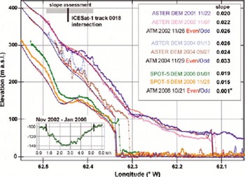
Slope changes along the glacier center line over the elevation-change anomaly provide some insight into the timing and causes of the abrupt elevation loss (Fig. 4). First, differencing elevation profiles from before and after the period of rapid elevation loss (ASTER, 7 November 2002 and SPOT-5, 1 January 2006) indicate a 4.5 km total extent of the region of anomalous elevation loss, with a maximum of 40m additional loss relative to areas upstream (98m loss) and downstream (103m loss; Fig. 4 inset). The 4.5 km along-flow region spanning the anomalous elevation-loss area shows a slightly increasing surface slope through time, from 0.020 in November 2001 (ASTER DEM prior to shelf breakup) to 0.026 in November 2002 (ATM profiles) as the post-shelf break-up effects propagate up-glacier. Slope across the region remains near that value in ASTER DEM longitudinal profiles in January 2004 (0.026) and September 2004 (0.024) that immediately precede the rapid elevation loss. The ATM profile of November 2004 shows an increased slope, to 0.033, at the onset of rapid elevation loss. Data from 2006 and later show much lower slopes, and a significantly changed profile. The October 2008 mean slope is 0.001. The ATM slope profiles track the development of the surface basin on the glacier, and independently confirm the changes seen in DEM differencing.

Fig. 4. Along-flow elevation profiles from ATM and satellite stereo-image DEMs for lower Crane Glacier, 2001–08. Red–blue line pairs for ATM data show the range of elevation variation across the swath of ATM laser measurements. Slope values in the inset table are the mean slope for a 4.51 km region defined by the difference of the November 2002 and January 2006 elevation profiles (lower left inset). Note that the ATM 2008 (asterisked) value is derived from a profile that deviated from the center line significantly (see Fig. 1).

A very large renewed acceleration of the glacier occurs at the same time (within months) as the sudden elevation loss over the anomaly and retreat of the ice front from the bedrock high (Fig. 5). Speed of the glacier at this site increases rapidly after loss of the ice shelf in early 2002, peaking at 710 ma^–1 in early 2003. Pre-shelf break-up speed in this region of the glacier has been estimated at 300 ma^–1 (Reference Rignot, Casassa, Gogineni, Krabill, Rivera and ThomasRignot and others, 2004). By late 2003, the glacier begins to slow again, to near 470ma^–1 (Fig. 5; see also Reference Hulbe, Scambos, Youngberg and LambHulbe and others, 2008).

Fig. 5. Elevation changes as in Figure 2, with flow speed changes over time superimposed (right-hand scale). Mean ice speed of the area at the intersection of ICESat-1 track 0018 and the ATM profiles (Fig. 1) was determined from image pair velocity mapping (Table 1). Horizontal bars for speed determinations represent the time between the image pair acquisitions. Errors in the speed determination are within the symbol size (<30ma^–1) except for the December 2002/February 2003 pair (±64ma^–1). Dates are month/day/year.

Attempts to use image correlation of image pairs straddling the period of anomalous elevation loss and the last stage of ice-front retreat to measure ice velocity failed because the glacier surface undergoes a large change during this period, dramatically increasing the density and intensity of crevassing. This change occurs over the entire lower trunk of the glacier (Fig. 6). In the SPOT-5 image pair used here just after the lake drainage event (January 2006 and November 2006; Table 1), a very large increase in speed is measured, roughly four times the pre-elevation loss (and pre-front retreat) speed (to 1943 ma^–1; Fig. 5). By early 2009, this decreased to 1430ma^–1, as measured by a Formosat-2 image pair (Reference Scambos and LiuScambos and Liu, 2009). A SPOT-5 image pair acquired in late 2009 and early 2010 yielded a speed of 1270ma^–1 in the anomaly region.

Fig. 6. ASTER (a, b) and SPOT-5 (c, d) image series showing crevasse changes in lower Crane Glacier spanning the period of inferred lake drainage, i.e. between scenes (b) and (c). Superimposed contours are flow speed from December 2002/February 2003 image pair (b), January 2006/November 2006 image pair (c), and the speed difference between the contour fields (d). See Table 1. SPOT-5 images copyright CNES (Centre National d’Études Spatiales, France)/distribution by SPOT image, SPIRIT project.

As noted above, in the months following the elevation change that began in September 2004, the glacier develops a dense crevasse network extending from near the ice front to 10km upstream (Fig. 6). Prior to this time, the glacier surface is relatively uncrevassed and gently undulating (Fig. 6a and b), despite the fact that it had already accelerated by a factor of 3–6 in the aftermath of the Larsen B ice shelf disintegration. The surface character is essentially unchanged between November 2002 and September 2004. As the anomalous elevation loss and most recent significant ice-front retreat begins in late 2004, the surface becomes covered in a dense network of crevasses at several orientations. This is particularly the case in the lowermost 2 km of the central glacier trunk, where the ice was observed to be afloat in 2006 (see Fig. 1), but the new dense crevasse pattern extends well upstream of the anomalous elevation-loss region. This new surface character persists through 2006 (Fig. 6c and d) and was observed on 2009 aircraft flights by one of the authors (C.A.S.).

To examine the potential causes of the secondary (2004–06) large acceleration and crevasse changes, we further analyzed the ice flow speed of a larger area of the lower Crane Glacier trunk using the best image pairs available (i.e. broadest clear-sky coverage) from the Figure 5 analysis. The selected image pairs for speed analysis in Figure 6 are given in Table 1. Figure 6b contains contours from the December 2002/February 2003 image pair. While this pair had a higher potential error for a single vector, the image features correlated very well, providing a dense vector field (~4500 vectors) that reduced the uncertainty of the velocity measurement (smoothing the grid by an inverse square algorithm with 600m×600m regions containing an average of 16 vectors each reduced the error reported in Table 1 by a factor of 4). The Figure 6b contours show that acceleration of the glacier in the aftermath of the 2002 Larsen B shelf disintegration was broad and uniform, with little evidence of local variations in basal or lateral shear. The longitudinal gradient in velocity is relatively constant. The 2006 image pair yielded fewer, less uniformly distributed vectors (2340 vectors) due to a rough surface and a longer time period between images. However, the mapped regions in the image pair (contours in Fig. 6c) show a very large additional acceleration of the glacier, roughly 2.5 times the previously mapped flow speed, i.e. an increase of 900–1250ma^–1. The 2006 mapping also shows a step in the velocity field, rising from 1400 to 1600ma^–1 in less than 1 km, at a location near the upper part of the elevation-loss anomaly. Differencing the two velocity fields (contours in Fig. 6d) indicates that the largest flow-speed increases occur on the flanks of the glacier, suggesting that the shear margins (the southern side in particular) have narrowed. Flow speed increased by up to a factor of 4 in that area by mid-2006.

4. Discussion

The highly localized nature of the elevation drawdown (Fig. 3), and the short temporal duration of the anomalous elevation-change event (Fig. 2), and the marked change in the along-flow profile (Fig. 4) lead us to conclude that the primary cause of the anomalous (greater than adjacent areas) elevation change across the center line of lower Crane Glacier was drainage of a kilometer-scale, relatively deep subglacial lake. The lake drainage period was between September 2004 and January 2006. Water depth drained from the subglacial reservoir was likely several tens of meters (Fig. 4 and inset). This subglacial lake appears to be in one of a series of subglacial lake basins in the Crane Glacier fjord, as revealed by the bathymetry (Fig. 1).

Other potential explanations, related to the rapidly changing ice dynamics of Crane Glacier after the loss of the Larsen B ice shelf, cannot fully account for the magnitude and localization of elevation loss over the feature (e.g. Reference Vieli and NickVieli and Nick, 2009). Recent ice models of Crane Glacier’s post-ice-shelf-loss responses do not show the anomaly, although they do adequately capture the changes in ice flow and broader changes in thickness and elevation elsewhere along the glacier (Reference Hulbe, Scambos, Youngberg and LambHulbe and others, 2008; Reference Vieli and NickVieli and Nick, 2009).

Estimating the size of the Crane subglacial lake is difficult. Reference Sergienko, MacAyeal and BindschadlerSergienko and others (2007) showed that ice-flow dynamics modify the surface expression of subglacial lake drainage, making it impossible to extract lake shape, size and volume from surface-measurable parameters. This is especially true in cases where the horizontal lake size is comparable to ice thickness. This appears to be the case for Crane Glacier, where ice thickness is of the order of 1000 m in the lower glacier trunk, and surface expression of the lake extends over 4.5 km along-flow and 2.2 km across-flow. In the Reference Sergienko, MacAyeal and BindschadlerSergienko and others (2007) model, moreover, it is shown that surface expression of lake drainage can be much larger than the area of the lake, especially along-flow, and that net surface lowering can be significantly less (in their modeled case, roughly one-third) than the actual depth of subglacial lake level drainage.

Given this, and in the absence of reliable data on ice thickness and bedrock shape, we can only make arbitrary, approximate estimates of the size and depth of the inferred Crane subglacial lake. We believe the following estimates of area and water-level change are conservative in view of the Reference Sergienko, MacAyeal and BindschadlerSergienko and others (2007) study. In Figures 3 and 4 we note the limit of significant surface drawdown anomaly (4.5×2.2 km), and in Figure 3 we mark the region of maximum gradient in the anomaly boundary (1.9×1.5 km). Assuming this smaller region is the approximate extent of the lake, and that water depth was on the order of 100 m (and therefore a volume of ~0.2 km³λ we explore the significance of the surface slope changes on the upper boundary of the lake, and the events leading to sudden drainage.

If the subglacial lake pressure is equilibrated with the overburden of ice directly above it, the slope of the ice/water interface is governed by a simple relationship related to the ice surface slope (i.e. the change in overlying ice thickness with horizontal distance) and the densities of ice and water:

where α is slope and ρ is density for the respective materials (Reference PatersonPaterson, 1994). Because surface slope changes with time across the elevation anomaly region, there is a change in the ice/water slope of the upper lake surface. In fact, the slope change at the roof of the lake would be a factor of 11 greater than the ice surface slope change, and in the opposite direction, if the water surface was in equilibrium everywhere with the local ice overburden.

Given the slope values in the table inset in Figure 4, and our approximation of lake size, this implies that the initial, pre ice-shelf break-up lake surface had ~420m relief (November 2001: 1.9km×0.020×11), rising from upstream to downstream. At the time of drainage, this would have increased to 690 m (November 2004: 1.9km×0.033 ×11). While it is unlikely that the ice above this lake was in full flotation equilibrium (Reference Sergienko, MacAyeal and BindschadlerSergienko and others, 2007), this illustrates that a surface slope change across a subglacially trapped water body has a large effect on its geometry.

As Crane Glacier’s slope steepened in response to loss of the ice shelf, the ice/water interface of the subglacial water body was tilted, raising the water level at the downstream boundary of the lake, i.e. at the obstruction to water flow that confined the lake. In our proposed scenario, the water level is raised until the obstruction is breached. The overlying ice was locally floated (i.e. hydraulically lifted) off the bedrock surface, and the lake volume was reduced by drainage. The dam may have been eroded by the drainage; alternatively, short-term details of the ice surface-slope change during drainage (e.g. a brief period of further steepening that is not captured by the series of profiles in Figure 4) pushed ~0.2 km³ of water over the dam.

The Crane Glacier dynamics-driven lake drainage process brings up an important consideration for a feedback for climate-driven outlet glacier changes. This process is likely to be applicable to any glacier with ponded subglacial water bodies, when the glacier is undergoing rapid dynamic changes, and therefore rapid surface slope changes. It is reasonable to suppose that many fjord-confined outlet glaciers have stable water bodies beneath them likely fed by a time-varying combination of surface and subsurface meltwater. In particular, the kinds of changes associated with climate warming (e.g. changes in the floating ice front, loss of contact with pinning points, loss of an ice shelf, or increased calving) accelerate the glacier, steepen its slope and thereby disturb the subglacial hydraulic pressure, pushing any trapped water into the subglacial system and thus reducing the basal shear stress (e.g. Reference ClarkeClarke, 2005). This inferred mechanism represents a special case of the several glacial floodwater flow mechanisms discussed by Reference RobertsRoberts (2005). The ‘type 4’ mechanism discussed there is flotation of a sealing ice dam by increased hydrostatic stress, and the inferred mechanism of increase is increased water pressure due to surface or subsurface melt input. Here we claim that the increase in hydrostatic stress was caused by changing surface slope, driving the subglacial water to stress levels that likely exceeded pre-shelf-break-up levels. Such drainage events may have a feedback effect on the glacier, causing a further acceleration and glacier steepening. Such a situation would pose a challenge for modeling of ice-sheet response to climate and ocean warming.

However, our study of the ice-flow speed change before and after the event (Fig. 6) shows that, in this case and perhaps generally, subglacial water drainage and movement produces relatively small changes in overall glacier speed, when compared to those caused by ice-front retreat or interactions with subglacial ridges or ice shelves. This pattern of rapid speed increase and slower decline, both in relative magnitude and in timing, matches the response characteristics of the similarly sized southeast Greenland glaciers Helheim and Kangerdlugssuaq (compare Fig. 5 to Reference Howat, Joughin and ScambosHowat and others, 2007; Reference Nick, Vieli, Howat and JoughinNick and others, 2009) as they dynamically responded to ice-front retreats.

The Crane Glacier case here offers an opportunity to test the relative impact of two near-simultaneous events: ice-front retreat from a bedrock ridge, and the drainage of a significant volume of water at mid-trunk, both initiated in late 2004. In Figure 6 the ice-speed contours and speed difference contours show that the far greater effect is a general acceleration of the entire lower trunk (Fig. 6c and d contours), both above and below the location of the lake. The dramatic crevasse-pattern changes confirm this, and extend across and upstream of the inferred lake area. Small features in the contours of ice-velocity change (Fig. 6d) near the upstream end of the lake indicated a ~20% net effect on flow speed change that may be associated with the subglacial lake drainage.

5. Conclusions

A rapid, localized elevation change in the lower central portion of Crane Glacier appears to be a result of subglacial lake drainage of a previously unknown lake beneath it. Source water for the lake was probably some combination of basal melting due to strain heating and surface meltwater that has drained through the ice upstream via hydro-fracturing. We do not yet observe any evidence for refilling, and the reservoir seal may be permanently compromised by the forced drainage. Bathymetric data and the discovery of sediments in basins within the newly opened fjord suggest that the new lake is one of a series of past subglacial water bodies. The Crane Glacier subglacial lake drainage was apparently triggered by surface slope changes along the glacier center line during glacier retreat (Fig. 4). Specifically, the retreat of the ice front from the subglacial ridge near 62.28˚ W in late 2004 (Fig. 1) appears to have caused a final further change in surface slope, that initiated rapid water discharge from the subglacial reservoir.

The pattern of ice-speed change, both temporally and spatially, supports the idea that glacier interaction with subglacial fjord topography and ice-front retreat across bedrock highs are the dominant control on ice flow and mass flux in outlet glaciers, and that subglacial water is of secondary importance. This high level of response to retreat from bedrock or pinning-point features has been identified for tidewater outlet glaciers everywhere (Reference Meier and PostMeier and Post, 1987; Reference Joughin, Rignot, Rosanova, Lucchitta and BohlanderJoughin and others, 2003; Reference Howat, Joughin and ScambosHowat and others, 2007; Reference JenkinsJenkins and others, 2008; Reference Nick, Vieli, Howat and JoughinNick and others, 2009). Conversely, subglacial hydrologic changes, even significant ones, are at most (to date) a 20% effect on outlet glacier speed (Reference Zwally, Abdalati, Herring, Larson, Saba and SteffenZwally and others, 2002b; Reference Joughin, Das, King, Smith, Howat and MoonJoughin and others, 2008; Reference Stearns, Smith and HamiltonStearns and others, 2008).