


1. Introduction
Roll waves exist in thin films of millimetre thickness and at depths of many metres in landslide mudflows and volcanic lava flows. This paper focuses on the large-scale roll wave instability affected mainly by inertia and gravity. We conduct direct numerical simulations (DNS) in this paper, solving the full Navier–Stokes equations for the nonlinear instability of the sheet flow of Newtonian fluid where the surface tension is negligible.
The aim of the present investigation differs from previous studies conducted for roll waves on film with a small thickness in the millimetre range affected mainly by surface tension. A teardrop smooth hump with short-wavelength capillary bow waves in front of the hump are characteristics of roll waves dominated by surface tension and viscosity (Kapitza Reference Kapitza1948; Julien & Hartley Reference Julien and Hartley1986; Liu, Paul & Gollub Reference Liu, Paul and Gollub1993; Alekseenko, Nakoryakov & Pokusaev Reference Alekseenko, Nakoryakov and Pokusaev1994; Liu & Gollub Reference Liu and Gollub1994; Nosoko et al. Reference Nosoko, Yoshimura, Nagata and Oyakawa1996; Ramaswamy, Chippada & Joo Reference Ramaswamy, Chippada and Joo1996; Malamataris, Vlachogiannis & Bontozoglou Reference Malamataris, Vlachogiannis and Bontozoglou2002; Gao, Morley & Dhir Reference Gao, Morley and Dhir2003; Park & Nosoko Reference Park and Nosoko2003).
On the other hand, gravity and inertia are the dominant influences in mudflow and debris-flow avalanches. Hungr, Morgan & Kellerhals (Reference Hungr, Morgan and Kellerhals1984) and Hungr (Reference Hungr1988) found debris flow at 1–5 metre depths in western Canada and Japan to be laminar, with apparent viscosity approximately  $3 \times 10^6$ times that of water. Hunt (Reference Hunt1994) analysed field and laboratory data, and concluded that the debris flows are Newtonian fluid flow in the laminar regime.
Giordano, Russell & Dingwell (Reference Giordano, Russell and Dingwell2008), Hui & Zhang (Reference Hui and Zhang2007), Giordano & Dingwell (Reference Giordano and Dingwell2003) and Giordano et al. (Reference Giordano, Mangiacapra, Potuzak, Russell, Romano, Dingwell and Di Muro2006) modelled volcanic magma and lava also as viscous Newtonian fluids. Giordano et al. (Reference Giordano, Russell and Dingwell2008) stated that the viscosity of natural silicate magmas generally spans from  $10^{-1}$ to $10^{14}$ Pa s, depending on the melt temperature and composition. The wave phenomena, such as regular hydraulic jump, undulating hydraulic jump, oblique hydraulic jump and standing waves, were observed in channelized lava flows during natural volcanic events (Finch & Macdonald Reference Finch and Macdonald1955; Takahashi & Griggs Reference Takahashi and Griggs1987; Wolfe et al. Reference Wolfe1988; Heslop et al. Reference Heslop, Wilson, Pinkerton and Head1989). Appendix A shows how and why debris torrents and volcanic magma can be modelled as laminar sheet flows with negligible surface tension.
Shkadov (Reference Shkadov1967) examined the laminar flow instability using a depth-averaged model including the surface tension. Ng & Mei (Reference Ng and Mei1994) formulated the theory of mudflow instability by extending Shkadov's model to power-law fluids, and found a ‘permanent roll waves’ solution between discontinuities using their shallow-layer formulation.
Other studies of roll waves were devoted to turbulent flow with quadratic friction (Jeffreys Reference Jeffreys1925; Dressler Reference Dressler1949; Brock Reference Brock1967; Zanuttigh & Lamberti Reference Zanuttigh and Lamberti2002; Balmforth & Mandre Reference Balmforth and Mandre2004; Que & Xu Reference Que and Xu2006; Richard & Gavrilyuk Reference Richard and Gavrilyuk2012; Ivanova et al. Reference Ivanova, Gavrilyuk, Nkonga and Richard2017; Yu & Chu Reference Yu and Chu2022, Reference Yu and Chu2023). Jeffreys (Reference Jeffreys1925) analysed the linear stability of turbulent sheet flow using a shallow-layer model, and found the critical Froude number  ${\textit {Fr}}=2$ – a critical Froude number very different from the value ${\textit {Fr}} = 0.527$ obtained by Yih (Reference Yih1955, Reference Yih1963) and Benjamin (Reference Benjamin1957) for laminar sheet flow. The hyperbolic equations of the shallow-layer model for the turbulent flow also produce solutions with mathematical discontinuities. Dressler (Reference Dressler1949) found the ‘permanent roll waves’ by matching the smooth profiles between discontinuities. Richard & Gavrilyuk (Reference Richard and Gavrilyuk2012) and Richard (Reference Richard2024) proposed supplemental energy and enstrophy equations in modelling the front of roll waves in turbulent flow, and found improved agreement with laboratory observation of the roll waves by Brock (Reference Brock1967).
One focus of the present study of the roll waves in the laminar sheet flow is the physics in a region immediately behind the wavefront. The other focus is examining the relationship between temporal and spatial instability. The temporal instability depends on a fixed wavelength specification. In spatial instability development, the prominent wave emerges as a front runner, which advances with increasing wavelength, wave amplitude and celerity. Yu & Chu (Reference Yu and Chu2022, Reference Yu and Chu2023) studied these problems in turbulent flow. This paper is about laminar flow of Newtonian fluid with negligible surface tension. In the DNS, we solve the Navier–Stokes equations using the volume of fluid (VOF) method. For comparison, we also conduct the simulation using the two-equation shallow-layer simulations (SLS) model of Ng & Mei (Reference Ng and Mei1994) and the four-equation shallow-layer weighted residual integral boundary layer (WRIBL) model of Ruyer-Quil & Manneville (Reference Ruyer-Quil and Manneville2000).
This paper has seven sections and four appendices, including this Introduction. Section 2 describes the formulation for DNS, the two-equation SLS model and the four-equation shallow-layer WRIBL model. Section 3 reviews the existing linear instability theories. Section 4 presents the simulations of the roll waves developed from temporal instability of a specified wavelength using a periodic boundary condition. The difference between the DNS and SLS is presented in this section using the analytical solution of Ng & Mei (Reference Ng and Mei1994) as a reference. Section 5 presents the spatial development of the roll waves. In this section, we determine the dependence of the celerity on the roll wave's amplitude. Section 6 examines a more accurate but still inadequate shallow-layer WRIBL model. Section 7 further explains the roll wave's spatial development versus its temporal development, and discusses the limitations of the two-equation and four-equation shallow-layer models. Appendix A explains why surface tension is negligible in geophysical debris and lava flows. Appendix B describes the adaptive quadtree mesh used in the DNS, and its refinement for numerical accuracy. Appendix C provides the computation details of the four-equation shallow-layer model. Appendix D evaluates the computation resources requirement for DNS compared with two-equation and four-equation shallow-layer approximations.
2. Formulation and numerical methods
We conduct DNS of the roll wave instability by solving the full Navier–Stokes equations using a two-phase VOF solver. The simulation starts from the initial instability of the sheet flow to the full nonlinear development of the roll waves. For comparison, we also conduct simulation using a two-equation SLS model of Ng & Mei (Reference Ng and Mei1994) and a four-equation WRIBL model by Ruyer-Quil & Manneville (Reference Ruyer-Quil and Manneville2000). Figure 1 shows two roll wave instability problems examined in this paper. Figure 1(a) shows the temporal development of the roll waves produced by a periodic disturbance. Figure 1(b) shows the spatial development of the roll waves produced by a localized disturbance.

Figure 1. (a) Periodic wave trains fully developed nonlinearly from temporal instability on an incline of angle  $\theta$ relative to the horizontal. (b) Wave packet characterized by the front runner (FR) developed from spatial instability. The dashed lines show the perturbation to the initial steady and uniform flow, which has depth $H$ and average depth velocity $U$. The four identical waves of wavelength $\lambda$ in (a) are initiated by periodic disturbance simulated using the periodic boundary conditions. On the other hand, the ‘wave packet’ and the front runner in (b) are developed from a localized disturbance near the inlet. The colour map shows the magnitude of the velocity $\sqrt {u^2+w^2}/U$, where $(u, w)$ are velocity components in the $x$- and $z$-directions, respectively.
2.1. Two-dimensional DNS
The governing equations for the DNS are
 $$\begin{gather} \frac{\partial u_i }{\partial x_i} =0, \end{gather}$$
 $$\begin{gather}\frac{\partial \rho u_i}{\partial t}+ \frac{ \partial \rho u_i u_j}{\partial x_j} =- \frac{\partial p}{\partial x_i} + \frac{\partial \tau_{ij}}{\partial x_j} + \rho g_i, \end{gather}$$
 $$\begin{gather}\frac{\partial \alpha}{\partial t}+ u_i\,\frac{\partial \alpha}{\partial x_i}=0, \end{gather}$$
where the  $i$ and $j$ subscripts follow Einstein's summation convention, $u_i$ is the velocity vector in the $x_i$-direction, and $g_i$ is the gravity component in the $x_i$-direction. The deviatoric stress tensor is related to the strain-rate tensor as follows:
 \begin{equation} \tau_{ij} = \mu \left(\frac{\partial u_i}{\partial x_j}+\frac{\partial u_j}{\partial x_i}\right), \end{equation}
where  $\mu$ is the dynamic viscosity. For a two-dimensional simulation of the flow down an incline shown in figure 1, the components of the velocity vector are $u_i = (u,w)$, and the components of gravity are $g_i= g (\sin \theta, \cos \theta )$ in the $x$- and $z$-directions, respectively. The volume fraction of the liquid $\alpha$, varying from 0 to 1, determines the volumetric average of density and viscosity as follows:
 $$\begin{gather} \rho = \alpha \rho_f +(1-\alpha){\rho_a}, \end{gather}$$
 $$\begin{gather}\mu =\left[ \frac{\alpha}{\mu_f} + \frac{1-\alpha}{\mu_a} \right]^{-1}, \end{gather}$$
where the subscripts  $f$ and $a$ refer to the liquid and air phases, respectively. Tryggvason, Scardovelli & Zaleski (Reference Tryggvason, Scardovelli and Zaleski2011) recommended the harmonic average as specified by (2.6) for large viscosity ratios. The piecewise linear interface calculation geometric VOF solver in the Basilisk platform (Popinet Reference Popinet2009; Popinet & Collaborators Reference Popinet2013–2024) determines the location of the air–liquid interface. The VOF scheme is momentum-conserving, enabling the momentum flux to be advected consistently with the mass flux (Fuster & Popinet Reference Fuster and Popinet2018; Zhang, Popinet & Ling Reference Zhang, Popinet and Ling2020), thus improving the computational robustness for cases with large density and viscosity ratios. The DNS are conducted using an adaptive quadtree mesh. The refined mesh has maintained within a less than 1 % computational error before wave breaking, according to the mesh refinement study in Appendix B. The accuracy of the simulation is not determined when the wave breaks randomly, entrapping air below the waves.
2.2. Two-equation SLS model
The two equations for the SLS are
 $$\begin{gather} \frac{\partial h}{\partial t} + \frac{\partial \bar{u} h}{\partial x} = 0, \end{gather}$$
 $$\begin{gather}\frac{\partial \bar{u}h}{\partial t} + \frac{\partial \left(\tfrac{6}{5} {\bar{u}^2}{h}+\tfrac{1}{2}g'h^2\right)}{\partial x} = g'hS_o - 3\,\frac{\mu}{\rho_f}\, \frac{\bar{u}}{h}, \end{gather}$$
where  $g^\prime =g\cos \theta$ is the reduced gravity on the slope, and $S_o= \tan \theta$ is the channel slope. The formulation for the two-equation SLS model assumes hydrostatic pressure distribution and self-similar parabolic velocity profiles:
 \begin{equation} {u} (z)= \frac{3}{2} \left[1- \left(1-\frac{z}{h}\right)^{2}\right] \bar{u} , \end{equation}
where  $\bar {u}=({1}/{h})\int _0^h {u}(z) \,{\rm d}z$ is the depth-averaged velocity. Ng & Mei (Reference Ng and Mei1994) developed the two-equation SLS model for power-law fluid to study landslide mudflow. The power-law index $n=1$ reduces the model to Newtonian laminar flow. Equations (2.7) and (2.8) form a hyperbolic equation set. They lead to mathematical discontinuities. The ‘permanent roll wave’ solution of Ng & Mei (Reference Ng and Mei1994) comprises the smooth-wave profiles connecting the discontinuities.
We conduct the SLS solving (2.7) and (2.8) on the Basilisk platform. The central-upwind scheme by Kurganov & Levy (Reference Kurganov and Levy2002) is used for spatial discretization. The method by Kurganov & Lin (Reference Kurganov and Lin2007) is adopted to reduce the numerical dissipation. The generalized MINMOD TVD limiter is employed for proper shock capturing, avoiding spurious numerical oscillation. The time integration scheme is a second-order predictor–corrector scheme. The details of the solver are elaborated in Popinet (Reference Popinet2011).
The two-equation SLS model is one-dimensional, involving only the  $\bar {u}$ velocity component. But the sheet flow can have $u$ and $w$ velocity components. Once disturbed, the pressure variation over the depth of the flow will no longer be hydrostatic, and velocity variation will not be parabolic in the region behind the wavefront.
2.3. Four-equation WRIBL model
More accurate one-dimensional shallow-layer models exist to account for the deviation of the velocity profile from the parabolic profile. One such model is the WRIBL model by Ruyer-Quil & Manneville (Reference Ruyer-Quil and Manneville2000). The model involves four equations, solving for depth  $h$, flow rate $q=\bar {u} h$, and two variables $s_1$ and $s_2$ introduced to account for deviation from the parabolic velocity profile. We conduct the WRIBL model simulation to compare with our DNS of roll waves using the open-source code WaveMaker by Rohlfs, Rietz & Scheid (Reference Rohlfs, Rietz and Scheid2018). The governing equations for the full second-order WRIBL model are complicated, involving lengthy equations with terms of up to third-order derivatives, and are not reproduced here. Interested readers could refer to (11), (38), (39) and (40) in Ruyer-Quil & Manneville (Reference Ruyer-Quil and Manneville2000).
Ruyer-Quil & Manneville (Reference Ruyer-Quil and Manneville2002) performed linear stability analysis and numerical simulation of thin film dominated by surface tension, and found good agreement of the WRIBL model with experiment, analytical solution and DNS up to  $Re=200$. However, to our knowledge, the WRIBL model has not been employed to study the sheet flow without surface tension.
2.4. The compatibility condition for steady and uniform undisturbed flow
The numerical simulation for the instability starts with an undisturbed sheet flow, which must be steady and uniform with a parabolic velocity profile given by (2.9). The depth and depth-averaged velocity of the undisturbed flow are  $H$ and $U$, respectively. The balance of the gravity driving force and the bed friction in the steady and uniform flow gives the relation
 \begin{equation} U= \frac{1}{3}\left[\frac{\rho g \sin{\theta}}{\mu}\,H^{2}\right], \end{equation}
which in dimensionless form is
 \begin{equation} {{\textit{Fr}}^2}=\tfrac{1}{3}\,{Re}\,S_o, \end{equation}
where  ${\textit {Fr}} = U/\sqrt {g'H}$ is the Froude number, and ${Re}=\rho UH/\mu$ is the Reynolds number. Equation (2.11) is a condition to ensure a steady and uniform undisturbed flow. Meaningful stability analysis must satisfy this compatibility condition. The result of DNS depends on any two of the three dimensionless parameters ${\textit {Fr}}$, $Re$ and $S_o$. However, the result of SLS depends only on ${\textit {Fr}}$ (Ng & Mei Reference Ng and Mei1994).
3. Linear instability theories
The instability of laminar sheet flow has been the subject of many studies. We summarize the neutral stability boundaries obtained from various approximations for their dependence on the Froude and Reynolds numbers, ignoring the surface tension effect.
3.1. The first-order long-wavelength approximation
Yih (Reference Yih1955, Reference Yih1963) and Benjamin (Reference Benjamin1957) analysed the linear instability of the sheet flow using a long-wavelength approximation of the Orr–Sommerfeld equations, and found that the Froude number needs to be smaller than the critical value  ${\textit {Fr}} = \sqrt {5/18} \approx 0.527$ as a requirement for stability of the laminar flow. Ng & Mei (Reference Ng and Mei1994) found the critical Froude number to be ${\textit {Fr}}= \sqrt {1/3} \approx 0.577$ using the two-equation shallow-layer model. The thick blue dashed line and blue dotted lines in figure 2 delineate the neutral stability boundaries of ${\textit {Fr}} = 0.527$ and 0.577, respectively.

Figure 2. The dependence of the neutral stability boundaries on Froude number and Reynolds number expressed in brown, green and purple colour according to (a) Chang & Demekhin (Reference Chang and Demekhin2002), (b) Lee & Mei (Reference Lee and Mei1996) and (c) Ruyer-Quil & Manneville (Reference Ruyer-Quil and Manneville2002), respectively. The thick curve is for the perturbation wavelength  $S_o\lambda /H=4.72$, while the thin curve is for a much shorter wavelength, $S_o\lambda /H=$ 0.472. The thick blue dashed line is the neutral stability boundary obtained by Yih (Reference Yih1955, Reference Yih1963), Benjamin (Reference Benjamin1957) and Ruyer-Quil & Manneville (Reference Ruyer-Quil and Manneville2002). The blue dotted line is the neutral stability boundary according to the two-equation shallow-layer model of Ng & Mei (Reference Ng and Mei1994). The thin grey dotted lines are the relation between ${\textit {Fr}}$ and $Re$ for a given $S_o$, according to the compatibility condition (2.11). The black open squares, red open circles and red solid circles denote the stable flows, non-breaking roll waves and breaking roll waves obtained from DNS for wavelength $S_o\lambda /H=4.72$.
The stability analysis of Yih (Reference Yih1955, Reference Yih1963) and Benjamin (Reference Benjamin1957), and the two-equation model of Ng & Mei (Reference Ng and Mei1994), were both first-order approximations in long-wavelength perturbation expansions. The neutral stability boundaries obtained from these first-order approximations depend only on the Froude number. However, the critical Froude number 0.577 obtained by the two-equation model is slightly greater than the correct value 0.527 because of the two-equation model assumption of hydrostatic pressure and unchanged parabolic velocity distribution over the depth of the laminar flow.
3.2. Higher-order long-wavelength approximation
Subsequent stability analyses by Chang & Demekhin (Reference Chang and Demekhin2002), Lee & Mei (Reference Lee and Mei1996) and Ruyer-Quil & Manneville (Reference Ruyer-Quil and Manneville2002) to higher orders of approximation have shown that stability also depends on the Reynolds number and the wavelength of the perturbation.
The neutral stability condition derived from the long-wavelength expansion of the Orr–Sommerfeld equation by Chang & Demekhin (Reference Chang and Demekhin2002) is
 \begin{equation} 4\,{Re}\,{ \sqrt{9009(-5+18\,{{\textit{Fr}}}^2) \left(\frac{S_o \lambda}{H}\right)^2+5{\rm \pi}^2} } = { 9 {\rm \pi}\sqrt{1\,107\,249} \, {{\textit{Fr}}}^2 } . \end{equation}
Lee & Mei (Reference Lee and Mei1996) captured the non-hydrostatic effect in their shallow-layer formulation, and obtained the following neutral stability condition:
 \begin{equation} {Re}\,{\sqrt{(-1+3\,{{\textit{Fr}}}^2) \left(\frac{S_o \lambda}{H}\right)^2}} = {6 {\rm \pi}\, \sqrt{\frac{14}{5}} \, {{\textit{Fr}}}^2 }. \end{equation}
The neutral stability condition by the simplified second-order WRIBL model of Ruyer-Quil & Manneville (Reference Ruyer-Quil and Manneville2002) is
 \begin{equation} {Re}\left(\frac{S_o\lambda}{H}\right) = 6{\rm \pi}\,\sqrt{\frac{3}{35}}\,{\textit{Fr}}^2\, \sqrt{\frac{-3\,{\textit{Fr}}^2+5 \sqrt{333\,{\textit{Fr}}^2+1470}\,{\textit{Fr}}+105}{18\,{\textit{Fr}}^2-5}}. \end{equation}
Equations (3.1), (3.2) and (3.3) are different in form from the original neutral stability conditions given in Chang & Demekhin (Reference Chang and Demekhin2002), Lee & Mei (Reference Lee and Mei1996) and Ruyer-Quil & Manneville (Reference Ruyer-Quil and Manneville2002). We eliminated the dependence of the original stability conditions on  $S_o$ using compatibility condition (2.11).
Figure 2 shows the neutral stability boundaries on the  ${\textit {Fr}}$– ${Re}$ plane. The grey dotted lines show the channel slope $S_o$ that satisfies the compatibility condition. The brown, green and purple colour lines in figures 2(a–c) represent (3.1), (3.2) and (3.3), respectively. The neutral stability condition depends on the wavelength of the perturbation. The thick and thin lines in the figure are neutral stability boundaries for the wavelength parameter $S_o \lambda /H= 4.72$ and 0.472, respectively. The selected wavelength $S_o \lambda /H= 4.72$ represents those roll waves observed in the laboratory by Julien & Hartley (Reference Julien and Hartley1986). On the other hand, the wavelength $S_o \lambda /H= 0.472$ represents the much shorter wavelength cases, with greater dependency on the wavelength and Reynolds number effects.
3.3. Stability dependence on wavelength and Reynolds number
The higher-order approximations have led to the roll wave instability dependence on the wavelength parameter  $S_o \lambda /H$ and the Reynolds number $Re$. As shown by the thick and thin curves in figure 2 of the neutral stability boundaries for the perturbation wavelengths $S_o\lambda /H=4.72$ and 0.472, the critical Reynolds numbers are approximately $Re_c \approx 4.50$ and 45.0, respectively. Therefore, the laminar sheet flow with a small Reynolds number $Re < 4.50$ would be stable to perturbation wavelengths shorter than $S_o\lambda /H=4.72$; even the Froude number is greater than the critical value 0.527 determined by the first-order approximation.
The laminar sheet flow is more unstable when perturbed by the longer wavelength of  $S_o\lambda /H=4.72$. The stability of the sheet flow depends only on the Froude number in the limiting case when the perturbation wavelength is infinitely long.
4. Temporal development of periodic roll waves
The hydrodynamic stability of sheet flow has been examined using linear and nonlinear theories. Assuming periodic disturbance, the eigenvalues of the linearized system of equations determine the initial exponential growth rate. The growth rate diminishes with the increase in the waves’ amplitude due to the nonlinear effect. The waves become fully developed, in equilibrium with the nonlinear effect, as the growth diminishes to zero.
4.1. The DNS for roll waves with  $S_o \lambda /H=4.72$

We conduct the DNS from the initial instability to the fully developed nonlinear roll waves, then compare the results with the permanent roll waves of Ng & Mei (Reference Ng and Mei1994). The simulation starts with a wavelength  $S_o \lambda /H=4.72$ perturbation to find the fully developed nonlinear waves when the growth rate diminishes to zero. Figure 3 shows the DNS compared with the SLS. The blue dashed lines in the figure outline the wave profiles obtained by SLS. The horizontal thin lines are the crest and trough of the permanent roll wave solution by Ng & Mei (Reference Ng and Mei1994).
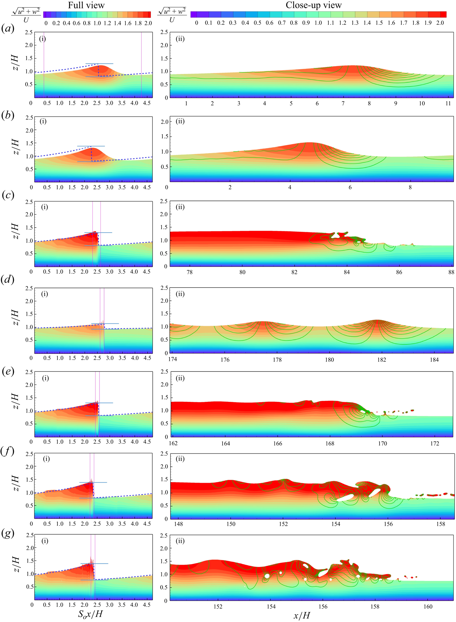
Figure 3. The periodic roll waves in a quasi-steady state developed from temporal instability. The colour maps show the velocity contours of the roll waves obtained from DNS. The blue dashed lines outline the wave profiles obtained by SLS. The horizontal thin lines are the crest and trough of the permanent roll wave solution by Ng & Mei (Reference Ng and Mei1994). The iso-lines for the  $w$ velocity component, denoted by the green curves on the right-hand side of the figure, show the significant uplifting velocity at the wavefront. Settings are (a i,ii) ${\textit {Fr}}=0.840$, $Re=5.88$, $S_o=0.360$; (b i,ii) ${\textit {Fr}}=1.10$, $Re=7.26$, $S_o=0.500$; (c i,ii) ${\textit {Fr}}=0.840$, $Re=70.6$, $S_o=0.0300$; (d i,ii) ${\textit {Fr}}=0.600$, $Re=72.0$, $S_o=0.0150$; (e i,ii) ${\textit {Fr}}=0.840$, $Re=141$, $S_o=0.0150$; (f i,ii) ${\textit {Fr}}=1.14$, $Re=260$, $S_o=0.0150$; (g i,ii) ${\textit {Fr}}=1.40$, $Re=392$, $S_o=0.0150$.
4.1.1. Stable cases
The temporal development of the waves depends on the wavelength parameter and the Reynolds number  $Re = \rho UH/\mu$ and the Froude number ${\textit {Fr}}=U/\sqrt {g^\prime H}$ of the base flow. The DNS amplitude diminishes to zero for the two cases with $({\textit {Fr}}, Re) = (0.840, 4.23)$ and $(1.10, 4.85)$. These two cases, denoted by the black open square symbols in the stability diagram figure 2, are on the stable side of the neutral stability boundary with $S_o \lambda /H=4.72$. Therefore, the diminishing DNS amplitude for these two cases agrees with the stability theories by Chang & Demekhin (Reference Chang and Demekhin2002), Lee & Mei (Reference Lee and Mei1996) and Ruyer-Quil & Manneville (Reference Ruyer-Quil and Manneville2002).
4.1.2. Unstable cases a, b, c, d, e, f and g
We also conduct DNS for cases on the unstable side of the neutral stability boundaries with  $S_o \lambda /H=4.72$. The Reynolds number and Froude number of these unstable cases labelled as a, b, c, d, e, f and g in figure 2 are $({\textit {Fr}}, Re) = (0.840, 5.88)$, $(1.10, 7.26)$, $(0.840, 70.6)$, $(0.600, 72.0)$, $(0.840, 141)$, $(1.14, 260)$ and $(1.40, 392)$, respectively. The perturbation amplitude of these unstable periodic disturbances increases with time and eventually approaches a fully nonlinear quasi-steady state when growth diminishes to zero. Figure 3 shows these fully nonlinear roll wave profiles in their quasi-steady state. The plots on the left-hand side of the figure show the roll waves over the entire wavelength from $S_ox/H=0$ to 4.72. The right-hand plots show the close-up views of the wavefronts in undistorted scales.
The wavefront in the left-hand plots of figure 3, expressed in terms of the compressed coordinate  $S_o x/H$, appears like a discontinuity, the amplitude of which closely agrees with the permanent roll wave solution of Ng & Mei (Reference Ng and Mei1994). However, in the close-up undistorted scales in the right-hand plots, the wavefront is either a multi-peaked undular bore or a single-peaked non-breaking or breaking wave.
4.2. The SLS and permanent roll waves
We also conducted the SLS to compare them with the DNS. The SLS profiles obtained from the hyperbolic model equations (2.7) and (2.8) shown as dashed lines in figure 3 are infinitely steep at the wavefront. The amplitudes of the wavefronts obtained by the SLS are in perfect agreement with the ‘permanent roll wave’ solution of Ng & Mei (Reference Ng and Mei1994) delimited between the blue horizontal thin lines in the figure.
On the other hand, the SLS for this case a, however, has produced a wave profile delineated by the blue dashed line, with depth  $\hat {h}_{SLS}=1.29$ at the wave crest, and depth $\check {h}_{SLS}=0.824$ at the wave trough, which are in perfect agreement with the permanent roll wave solution of Ng & Mei (Reference Ng and Mei1994) delimited between the blue horizontal thin lines, because the Froude number ${\textit {Fr}} = 0.840$ in this case is greater than the critical value 0.577 according to the one-dimensional two-equation model of Ng & Mei (Reference Ng and Mei1994).
4.3. Smooth wavefronts and undular bore for marginally unstable cases a, b and d
The difference between the DNS and SLS profiles occurs mainly at the wavefront, where the long wavelength approximation breaks down. The wavefront is smooth and gradually varying for the marginally unstable cases a and b, where the Reynolds number is slightly greater than the critical value, which is slightly above the neutral stability boundaries as shown in figure 2. Figures 3(a) and 3(b) show the smooth wavefronts with the roll wavefront amplitude slightly smaller than in the SLS model.
The other significant difference between the DNS and SLS is the profile for the marginally unstable case d. The Froude number of this case is  ${\textit {Fr}} = 0.600$, which is higher but very close to the critical value ${\textit {Fr}}_c=$ 0.527. However, the Reynolds number for this case, $Re = 72$, is quite large. The profile behind the wavefront in this marginally unstable case, with a large Reynolds number, is the in the multi-peaked undular bore profile as shown in figure 2(d).
4.4. Breaking wavefront for unstable cases c, e, f, and g
The sheet flows in cases d, e, f and g are on the same slope  $S_o=0.0150$. The frontal region of case d is a multi-peaked undular bore. As the Froude number increases from ${\textit {Fr}} = 0.600$ to 0.840, 1.14 and 1.40, away from the critical value 0.527, the wavefronts in cases c, e, f and g become progressively more chaotic, as shown in figures 2(c) and 2(e–g). We identify the smooth waves using open circle symbols, and breaking waves using solid circle symbols, in figure 2.
The breaking wavefront shows the entrainment of air bubbles. The process of air entrapment is chaotic. The present level of mesh refinement predicts the initiation of breaking and the bulk of the roll wave but may not correctly simulate the detailed chaotic process of air entrapment.
4.5. The perturbation wavelength associated with the temporal analysis
The simulation cases from a to g presented in figure 3 are for a specified perturbation wavelength parameter  $S_o \lambda /H = 4.72$. The results would be different, and the neutral stability boundary would be the thin curves in figure 2, if we had selected a much shorter wavelength $S_o \lambda /H =0.472$. Cases a and b would become stable, and cases c and d become marginally unstable because cases a and b would be on the stable side of the neutrally stable boundaries for $S_o \lambda /H = 0.472$, which are the thin curves in figure 2.
On the other hand, if the perturbation wavelength is infinitely long, then the stability of laminar sheet flow would depend only on the critical Froude number. The flow will become unstable due to the disturbance of infinitely long wavelength as long as the Froude number exceeds the critical value  ${\textit {Fr}}_c=0.527$ – unaffected by the Reynolds number.
5. Spatial development of the front runner produced by localized disturbances
The classical hydrodynamic stability theory derived from the normal-mode approach assumes periodic disturbance, which leads to periodic roll waves, whose amplitudes are not determined until the wavelength is specified. The permanent roll waves by Ng & Mei (Reference Ng and Mei1994) also depend on the wavelength.
To overcome this difficulty of indeterminacy, Yu & Chu (Reference Yu and Chu2022, Reference Yu and Chu2023) studied the spatial development of roll waves produced by a localized disturbance, focusing on the dominant leading waves – the front runner. The works of Yu and Chu were for the turbulent flow of clear waters.
We conduct DNS for the spatial development of the roll waves on the laminar sheet flow, initiated by localized disturbance at the inlet, then follow the growth of the disturbance for a series of unstable sheet flows of undisturbed Froude number  ${\textit {Fr}} = 0.70$, 0.84 and 1.00. The corresponding undisturbed flow Reynolds numbers of these unstable sheet flows are $Re = 98.0$, 35.3 and 50.0, and the channel slopes are $S_o=0.015$, 0.06, 0.06, respectively. The Froude number ${\textit {Fr}}$, the Reynolds number $Re$, and the channel slope $S_o$ are selected for the simulation to satisfy the compatibility equation (2.11) so that gravity is in balance with the bed friction stress in the undisturbed base flow, which is steady and uniform flow.
The most prominent roll wave in spatial development is the front runner, which leads the waves in the packet developed from instability. Yu & Chu (Reference Yu and Chu2022) studied the front runner in turbulent sheet flow. The front runner in a wave packet was also observed in a mudflow simulation by Liu & Mei (Reference Liu and Mei1994) and by Meza & Balakotaiah (Reference Meza and Balakotaiah2008), who studied the nonlinear waves on vertically falling films dominated by viscosity and surface tension. Meza & Balakotaiah (Reference Meza and Balakotaiah2008) used the word ‘tsunami’ in exaggeration to describe the front runner in their study of the falling film.
Figures 4, 5, 6 and 7 show the development of the front runner. The depth  $h_{FR(DNS)}$ and the depth-averaged velocity $\bar {u}_{FR(DNS)}$ of the front runner obtained from DNS are compared with the corresponding results $h_{FR(SLS)}$ and $\bar {u}_{FR(SLS)}$ obtained from SLS in a table at the bottom of each figure. On the left-hand sides of the figures, the depth and velocity profiles are on the compressed coordinate $S_ox/H$. The right-hand sides show the close-up profiles of the front runner on the undistorted scales.

Figure 4. The development of the front runner produced by a localized disturbance at the inlet on an unstable sheet flow with  ${\textit {Fr}}=0.560$, ${Re}=15.7$ and $S_o=0.060$. The colour maps show the DNS results, while the blue dashed lines denote the free-surface profiles obtained by the SLS. The green curves are iso-lines for the $w$ velocity component. Here: (a i,ii) $S_ot_{DNS}U/H=4.25$, $S_ot_{SLS}U/H=3.94$; (b i,ii) $S_ot_{DNS}U/H=8.50$, $S_ot_{SLS}U/H=8.02$; (c i,ii) $S_ot_{DNS}U/H=12.8$, $S_ot_{SLS}U/H=12.2$; (d i,ii) $S_ot_{DNS}U/H=17.0$, $S_ot_{SLS}U/H=16.4$; (e i,ii) $S_ot_{DNS}U/H=21.3$, $S_ot_{SLS}U/H=20.6$.

Figure 5. The development of the front runner produced by a localized disturbance at the inlet on an unstable sheet flow with  ${\textit {Fr}}=0.700$, ${Re}=98.0$ and $S_o=0.0150$. The colour maps show the DNS results, while the blue dashed lines denote the free-surface profiles obtained by the SLS. The green curves are iso-lines for the $w$ velocity component. Here: (a i,ii) $S_ot_{DNS}U/H=2.00$, $S_ot_{SLS}U/H=1.87$; (b i,ii) $S_ot_{DNS}U/H=4.00$, $S_ot_{SLS}U/H=3.77$; (c i,ii) $S_ot_{DNS}U/H=6.00$, $S_ot_{SLS}U/H=5.68$; (d i,ii) $S_ot_{DNS}U/H=8.00$, $S_ot_{SLS}U/H=7.61$; (e i,ii) $S_ot_{DNS}U/H=10.0$, $S_ot_{SLS}U/H=9.54$.

Figure 6. The development of the front runner produced by a localized disturbance at the inlet on an unstable sheet flow with  ${\textit {Fr}}=0.840$, ${Re}=35.3$ and $S_o=0.0600$. The colour maps show the DNS results, while the blue dashed lines denote the free-surface profiles obtained by the SLS. The green curves are iso-lines for the $w$ velocity component. Here: (a i,ii) $S_ot_{DNS}U/H=4.60$, $S_ot_{SLS}U/H=4.32$; (b i,ii) $S_ot_{DNS}U/H=9.20$, $S_ot_{SLS}U/H=8.74$; (c i,ii) $S_ot_{DNS}U/H=13.8$, $S_ot_{SLS}U/H=13.2$; (d i,ii) $S_ot_{DNS}U/H=18.4$, $S_ot_{SLS}U/H=17.8$; (e i,ii) $S_ot_{DNS}U/H=23.0$, $S_ot_{SLS}U/H=22.3$.

Figure 7. The development of the front runner produced by a localized disturbance at the inlet on an unstable sheet flow with  ${\textit {Fr}}=1.00$, ${Re}=50.0$ and $S_o=0.0600$. The colour maps show the DNS results, while the blue dashed lines denote the free-surface profiles obtained by the SLS. The green curves are iso-lines for the $w$ velocity component. Here: (a i,ii) $S_ot_{DNS}U/H=4.80$, $S_ot_{SLS}U/H=4.53$; (b i,ii) $S_ot_{DNS}U/H=9.60$, $S_ot_{SLS}U/H=9.13$; (c i,ii) $S_ot_{DNS}U/H=14.4$, $S_ot_{SLS}U/H=13.8$; (d i,ii) $S_ot_{DNS}U/H=19.2$, $S_ot_{SLS}U/H=18.4$; (e i,ii) $S_ot_{DNS}U/H=24.0$, $S_ot_{SLS}U/H=23.2$.
The front runner development is not dependent on the form of the inlet disturbance. Yu & Chu (Reference Yu and Chu2022) examine the instability due to six types of localized disturbances. For the present simulation, the disturbance is ‘type c of constant  ${\textit {Fr}}$’, which, according to Yu & Chu (Reference Yu and Chu2022), is a small rise in depth in the form of a half-sinusoid, and at the same time a slight increase in velocity to keep the disturbance Froude number ${\textit {Fr}}$ unchanged.
To reproduce the wave packet from the instability, we introduced a localized perturbation to the uniform flow. The depth-averaged initial perturbation at  $t=0$ is
 $$\begin{gather} h(x, t=0)= \begin{cases} H\left[1+\epsilon\sin\left(\dfrac{2{\rm \pi} x}{\ell}\right)\right] & {\rm for}\ 0< x\leq\dfrac{\ell}{2},\\ H & {\rm for} \ x > \dfrac{\ell}{2}, \end{cases} \end{gather}$$
 $$\begin{gather}\bar{u} (x, t=0 ) = {\textit{Fr}}\,\sqrt{g' [h(x,t=0) ]^3}. \end{gather}$$
 The depth of the initial disturbance  $h(x, t=0)$, is the upper half of a sinusoid of length $\ell$ raised to an amplitude $\epsilon$ over the extent $0< x\leq {\ell }/{2}$, while $\bar {u}$ is selected to keep the Froude number of the disturbance equal to the Froude number of the undisturbed flow. This initial perturbation defined by (5.1) is similar to the ‘type c disturbance of constant ${\textit {Fr}}$’, which is one of the six inlet disturbances examined by Yu & Chu (Reference Yu and Chu2022) and Yu & Chu (Reference Yu and Chu2023), who found that all six produced the same front runner.
For DNS, we assume parabolic variation of velocity over the depth. The initial profiles for  $\alpha$, $u$ and $w$ are
 $$\begin{gather} \alpha(x, z, t=0)= \begin{cases} 1 & {\rm for} \ 0< z\leq h(x, t=0),\\ 0 & {\rm for} \ z>h(x, t=0), \end{cases} \end{gather}$$
 $$\begin{gather}u (x, z, t=0 ) = \begin{cases} \dfrac{3}{2} \, \bar{u} (x, t=0 ) \left[1-\left(1-\dfrac{z}{h(x, t=0)}\right)^2 \right] & {\rm for} \ 0< z\leq h(x,t=0),\\[10pt] \dfrac{3}{2} \, \bar{u} (x, t=0 ) & {\rm for} \ z>h(x, t=0), \end{cases} \end{gather}$$
 $$\begin{gather}w (x, z, t=0 ) = 0. \end{gather}$$
 The front runner is not sensitive to the amplitude and length of the initial inlet disturbance, as demonstrated in the previous papers by Yu & Chu (Reference Yu and Chu2022, Reference Yu and Chu2023). For the simulations shown in figures 4, 5, 6 and 7,  $\epsilon =0.2$ and $S_o\ell /H =2$.
5.1. Profile of the front runner
Depending on the Froude and Reynolds numbers, the front runner can be a multi-peaked undular bore or a single-peaked non-breaking or breaking wave. However, according to the SLS model, the wavefront is nothing but a discontinuity.
The front runner for the case  $({\textit {Fr}}, Re) = (0.56, 15.7)$ shown in figure 4 has a smooth wavefront. The case $({\textit {Fr}}, Re) = (0.70, 98.0)$ shown in figure 5 has a smooth frontal region in the form of an undular bore.
For the higher Froude number cases with  $({\textit {Fr}}, Re) = (0.84, 35.3)$ and $(1.00, 50.0)$ shown in figures 6 and 7, the steep wavefront eventually breaks, entrapping air in the form of a plunging wave breaker. The process of breaking is somewhat chaotic. The Reynolds number of the front runner is as large as $Re_{FR(DNS)}={\rho h_{FR}\bar {u}_{FR}}/{\mu }=218$ nearly in the transition from laminar to turbulent flow in these high Froude number cases. The laboratory observation of laminar falling films by Adomeit & Renz (Reference Adomeit and Renz2000) has found isolated turbulent spots interacting with surface waves at Reynolds numbers varying from 75 to 200. The wave breaking and entrapment of air in the front runner are chaotic, as shown in figures 6(e) and 7(e). Further mesh refinement would be required to resolve the turbulent spots (if any) in our DNS.
The table at the bottom of each figure provides the critical data obtained from the simulations. The front runner velocity obtained by DNS,  ${u}_{FR(DNS)}$, is approximately 2 % larger than the velocity ${u}_{FR(SLS)}$ obtained by SLS.
For the case shown in figure 6, the front runner Froude numbers are  ${\textit {Fr}}_{FR(DNS)} =\bar {u}_{FR}/\sqrt {g' h_{FR}}=0.909$, 1.04, 1.15, 1.32 and 1.54, and the front runner Reynolds numbers are $Re_{FR(DNS)} ={\rho h_{FR}\bar {u}_{FR}}/{\mu }=64.0$, 79.9, 95.5, 121 and 164, at front runner positions $S_ox_{FR}/H=13.8$, 26.8, 40.6, 55.3 and 71.7, respectively. A breaking wave is observed to occur as the front runner advances to a position $S_ox_{FR}/H=40$, beyond which the motion progressively becomes chaotic.
For the case shown in figure 7, the front runner Froude numbers are  ${\textit {Fr}}_{FR(DNS)} =1.20$, 1.26, 1.32, 1.42 and 1.54, and the front runner Reynolds numbers are $Re_{FR(DNS)} = 107$, 122, 143, 173 and 218, at front runner positions $S_ox_{FR}/H=13.5$, 26.2, 39.8, 54.4 and 70.3, respectively. At position $S_ox_{FR}/H=70.3$, the front runner Froude number in this case has value ${\textit {Fr}}_{FR(DNS)} = 1.54$, which is getting close to the critical Froude number ${\textit {Fr}} = 2.0$ for turbulent roll waves according to the stability analysis of Jeffreys (Reference Jeffreys1925).
5.2. The front runner's depth and velocity
The velocity of the front runner  $\bar {u}_{FR}/U$ increases with its depth $h_{FR}/U$ following closely a linear relationship as shown in figure 8. The strong linear dependence of velocity on depth is observed in debris flow, and it has been used by Hungr et al. (Reference Hungr, Morgan and Kellerhals1984) and Wu et al. (Reference Wu, Kang, Tian and Zhang1990) to show debris flow to be in a laminar regime.

Figure 8. The front runner's depth  $h_{FR}/H$ and its relation to the velocity $\bar {u}_{FR}/U$ for (a) ${\textit {Fr}} = 0.56$ ( $Re = 15.7$, $S_o=0.060$), (b) ${\textit {Fr}} = 0.70$ ( $Re = 98.0$, $S_o=0.015$), (c) ${\textit {Fr}} = 0.84$ ( $Re = 35.3$, $S_o=0.060$) and (d) ${\textit {Fr}} = 1.00$ ( $Re = 50.0$, $S_o= 0.060$).
5.3. Front runner's celerity–amplitude relationship
The celerity of the front runner depends on wave amplitude. Figure 9 shows the celerity–amplitude relationship. We use the front runner's depth-averaged speed  $\bar {u}_{FR}/U$ to represent its amplitude, and the celerity $c_{FR}/U$ is related to the front runner's amplitude $\bar {u}_{FR}/U$. The DNS results all follow approximately a linear relationship denoted by the dashed lines in the figure. The SLS produces slightly different trends. The front runner is the most prominent wave because it advances faster than all trailing waves. It is destructive because the wave advances at a celerity speed greater than the base flow.

Figure 9. The front runner's celerity  $c_{FR}/U$ and its dependence on the speed of the front runner $\bar {u}_{FR}/U$ for (a) ${\textit {Fr}} = 0.56$ ( $Re = 15.7$, $S_o=0.060$), (b) ${\textit {Fr}} = 0.70$ ( $Re = 98.0$, $S_o= 0.015$), (c) ${\textit {Fr}} = 0.84$ ( $Re = 35.3$, $S_o=0.060$) and (d) ${\textit {Fr}} = 1.00$ ( $Re = 50.0$, $S_o=0.060$).
The square symbol in the figure denotes the limiting condition when  $c_{FR}=U+\sqrt {g'H}$ and $\bar {u}_{FR}/U = 1$. The dashed line traces back to the square symbol. For ${\textit {Fr}} = 0.56$, 0.70, 0.84 and 1.00, the slopes of the dashed lines are ${\rm d} c_{FR}/{\rm d} \bar {u}_{FR}=1.10$, 1.21, 1.18 and 1.15, which are nearly constant. The corresponding limiting conditions are ( $c_{FR}/U, \bar {u}_{FR}/U) = (1+{{\textit {Fr}}}^{-1}, 1)=(2.79, 1)$, $(2.43, 1)$, $(2.19, 1)$ and $(2.00, 1)$.
The dependence of celerity on amplitude explains the existence of the front runner. The dominant wave with the most significant amplitude advances with the maximum celerity among the waves, and emerges from the pack of waves as the front runner.
Yu & Chu (Reference Yu and Chu2022) found that the turbulent roll wave has similar celerity–amplitude relations. Meza & Balakotaiah (Reference Meza and Balakotaiah2008) studied the dynamics of nonlinear large-amplitude waves on vertically falling films for viscosity and surface tension effects. The celerity–amplitude relationships of the vertical falling films also follow approximately linear relationships, independent of the forcing frequency and amplitude of the disturbance introduced at the inlet. The similarity in the production of waves due to nonlinear instability between our laminar sheet flow, the turbulent sheet flow studied by Yu & Chu (Reference Yu and Chu2022) and the vertical falling film problem by Meza & Balakotaiah (Reference Meza and Balakotaiah2008) is remarkable – despite the difference in inertia, gravity, viscosity and surface tension effects between these problems.
5.4. Bed friction and uplifting velocity at the wavefronts
The difference in results between DNS and SLS occurs mainly in the frontal region of the roll wave where, strictly speaking, the long-wavelength approximation fails. One parameter of significance is the bed friction  $\tau _b=[\mu (\partial u/\partial z)]|_{z=0}$. The other is the $w$ velocity component, which also is significant in the frontal region. The $w$ velocity occurs mainly near the free surface. Searching for the maximum $w$ velocity over the depth gives the ‘uplifting velocity’ $\hat {w}$. The significant increases in bed friction and uplifting velocity are also the characteristics of breaking shallow-water waves in a tank (Perlin, He & Bernal Reference Perlin, He and Bernal1996; Mostert & Deike Reference Mostert and Deike2020; Liu et al. Reference Liu, Wang, Bayeul-Lainé, Li, Katz and Coutier-Delgosha2023).
Figure 10 shows the variation of the bed-friction shear stress  $\tau _{b}$ relative to the undisturbed $\overline {\tau _b}$, $\tau _{b}/\overline {\tau _b}$, in the frontal region over a distance from $(x-x_{FR})/H=-30$ to 10. The blue solid line in the figure shows the bed-friction shear stress obtained by DNS. The red dashed line is the bed friction significantly underestimated by SLS. The SLS model may produce a profile for the bulk body of the roll wave, but is inadequate in describing the roll wave's frontal region. The inability to predict bed-friction shear stress correctly is due to the assumed self-similar parabolic velocity profile in formulating the SLS model.

Figure 10. The bed-shear stress  $\tau _b/\overline {\tau _b}$ profiles near the wavefronts for the simulation cases (a) ${\textit {Fr}}=0.700$, ${Re}=98.0$ ( $S_o=0.0150$), (b) ${\textit {Fr}}=0.840$, ${Re}=35.3$ ( $S_o=0.0600$), (c) ${\textit {Fr}}=1.00$, ${Re}=50.0$ ( $S_o=0.0600$) shown in figures 5, 6 and 7, respectively. The blue solid lines and red dashed lines denote the DNS and SLS results, respectively.
The tables at the bottom of figure 10 provide the peak values of the bed friction obtained from DNS and SLS. The DNS give the relative bed friction varying from  $\hat {\tau }_{b(DNS)}/\overline {\tau _b} = 1.37$ to 1.95. The substantial increase of bed friction in the frontal region suggests the need for an accurate model to study soil erosion in debris flow and avalanche.
Figure 11 shows the uplifting velocity  $\hat {w}/U$ profile in the frontal region obtained from DNS. The uplifting velocity rises sharply before the breaking of the waves. It then becomes slightly chaotic with the air entrapment by the plunging breaker. The uplifting velocity can be upwards (positive) or downwards (negative) after the breaking. The SLS model could not predict the breaking of the wave without the $w$ velocity component in the model.

Figure 11. The peak uplifting velocity  $\hat {w}/U$ profile near the wavefronts for the simulation cases (a) ${\textit {Fr}}=0.700$, ${Re}=98.0$ ( $S_o=0.0150$), (b) ${\textit {Fr}}=0.840$, ${Re}=35.3$ ( $S_o=0.0600$), (c) ${\textit {Fr}}=1.00$, ${Re}=50.0$ ( $S_o=0.0600$) shown in figures 5, 6 and 7, respectively.
5.5. Length of the frontal region
The wavefront is a region of excessive bed-friction stress and uplifting velocity. The profiles of  ${\tau }_b^{(DNS)}/\overline {\tau _b}$ and $\hat {w}/U$ denoted by the blue lines in figures 10 and 11 show that the excessive bed friction and uplifting velocity occur over the length varying from $(x-x_{FR})/H \approx -10$ to 0. Therefore, the length of the frontal region is approximately $10 H$, ten times the depth of the undisturbed flow.
5.6. Front runner velocity and pressure variation over the depth
The velocity variation over the depth in the frontal region is not precisely parabolic, and the pressure is not hydrostatic. Figures 12(a)–12(c) show the velocity profiles, while figures 12(d–f) show the corresponding DNS pressure profiles at the front runner obtained by the DNS. The dashed lines are the profiles of the undisturbed flow.

Figure 12. The front runner velocity  $u_{FR}/\bar {u}_{FR}$ as a function of $z/h_{FR}$, and front runner pressure $p_{FR}/(\rho g^\prime H)$ as a function of $z/h_{FR}$ obtained by DNS. The dashed line delineates the reference profile of the undisturbed flow. (a–c) The velocity profiles; (d–f) the pressure profiles, for (a,d) ${\textit {Fr}}=0.70$, ${Re}=98$, $S_o=0.015$, (b,e) ${\textit {Fr}}=0.84$, ${Re}=35$, $S_o=0.060$, and (c,f) ${\textit {Fr}}=1.0$, ${Re}=50$, $S_o=0.060$.
The front runner region's DNS velocity deviates slightly from the parabolic profile given by (2.9). The velocity gradient near the channel bed exceeds the undisturbed flow, leading to higher bed-friction stress in the region near the wavefront.
The vertical pressure distribution obtained by DNS is approximately linear. However, the value  $p_{FR}/(r g^\prime h_{FR})$ at the bottom is slightly smaller than unity, which reflects the effect of the vertical uplift velocity and air entrapment at the wavefront of the front runner.
6. Four-equation WRIBL model
Ruyer-Quil & Manneville (Reference Ruyer-Quil and Manneville2000) introduced an accurate four-equation WRIBL model. We perform the WRIBL model simulation using the open-source code WaveMaker by Rohlfs et al. (Reference Rohlfs, Rietz and Scheid2018). The WRIBL model equations have many high-order derivative terms. Therefore, the spectral method is used for spatial discretization to guarantee simulation convergence, while a fifth-order Runge–Kutta adaptive scheme is used for time integration.
Figures 13 and 14 show the close-up profiles near the wavefronts for the velocity and bed-shear stress in the region near the wavefront, obtained by DNS, two-equation SLS and four-equation WRIBL model simulation for the cases  ${\textit {Fr}}=0.600$, ${Re}=72.0$ ( $S_o=0.0150$) and ${\textit {Fr}}=0.840$, ${Re}=141$ ( $S_o=0.0150$), respectively. The simulation was conducted for the temporal development with a periodic boundary condition over one wavelength $S_o \lambda /H=4.72$. Appendix C provides the profiles over the entire wavelength obtained from the simulations.

Figure 13. The close-up profiles in the region near the wavefront obtained from (a,d) DNS, (b,e) full second-order SLS, and (c,f) WRIBL simulation, for  ${\textit {Fr}}=0.600$, ${Re}=72.0$ ( $S_o=0.0150$). (a–c) Velocity contours; (d–f) bed-friction stress profiles.

Figure 14. The close-up profiles in the region near the wavefront obtained from (a,d) DNS, (b,e) two-equation SLS, and (c,f) the four-equation WRIBL model simulation, for  ${\textit {Fr}}=0.840$, ${Re}=141$ ( $S_o=0.0150$). (a–c) Velocity contours; (d–f) bed-friction stress profiles.
Despite the improvement in predicting the bed-friction stress at the wavefront as shown in figures 13(f) and 14(f), the four-equation WRIBL model still does not produce the undular bores and wave breaking predicted by the DNS shown in figures 13(a) and 14(a), respectively. The WRIBL model agrees better with DNS than with SLS. However, the WRIBL simulation wavefront is too steep, unlike any profiles predicted by the DNS.
7. Summary and conclusion
We conduct numerical simulations (DNS) to study roll waves’ temporal and spatial development on a laminar sheet flow with negligible surface tension. The DNS results are compared with the two-equation shallow-layer simulation (SLS) and the four-equation WRIBL model to determine the limitations of these approximation models.
The DNS for temporal development are to show consistency with existing theories of roll waves with different orders of approximations. The existing linear stability theories developed using the normal mode approach are for disturbance of a specified wavelength. The ‘permanent roll wave’ solution obtained by Ng & Mei (Reference Ng and Mei1994) also depends on the wavelength.
Roll waves’ spatial development is the primary focus of our DNS study. The spatial development depends not on wavelength specification but on Froude number and distance away from the localized disturbance. Our DNS form the first-ever study of the spatial development of the roll waves on laminar sheet flow with negligible surface tension. The front runner in the spatial development can be a multi-peaked undular bore or a single-peaked non-breaking or breaking wave. The bed friction is significant in the frontal region of the front runner. The frontal length with significant bed friction and uplifting velocity is approximately ten times the undisturbed flow depth.
The two-equation SLS model has produced the bulk profile of roll waves with the least computational cost among the three models. The model fails to predict the significant increase in bed friction in the frontal region of the wave. It slightly underestimates the roll wave amplitude and velocity compared with DNS. Much effort has been made to improve the two-equation shallow-layer model. Ruyer-Quil & Manneville (Reference Ruyer-Quil and Manneville2000) have proposed a hierarchy of shallow-layer models with different degrees of simplification. Their four-equation shallow-layer model can better predict the frontal region's bed friction. The two-equation SLS model by Ng & Mei (Reference Ng and Mei1994), and the four-equation WRIBL model, are both one-dimensional models, solving the  $\bar {u}$ component of velocity. These one-dimensional models, however accurate they may be, cannot produce the undular bore or wave breaking phenomena correctly.
The present simulation of the laminar sheet flow ignores surface tension. The results are therefore not comparable to small-scale laboratory experiments by Julien & Hartley (Reference Julien and Hartley1986) and Liu & Gollub (Reference Liu and Gollub1994). However, surface tension should be negligible in large-scale geophysical flow where gravity and inertia are the dominant influences. Hunt (Reference Hunt1994), for example, has suggested modelling debris flow using a Newtonian model of laminar sheet flow. The modelling of mudflow with negligible surface tension, such as in the works of Ng & Mei (Reference Ng and Mei1994), Liu & Mei (Reference Liu and Mei1994) and Balmforth & Liu (Reference Balmforth and Liu2004), are closely related to the laminar sheet examined in this paper.
We found that the celerity of the roll waves in laminar sheet flow depends on the waves’ amplitude following a linear relationship. Yu & Chu (Reference Yu and Chu2022) found that the turbulent roll wave has similar celerity–amplitude relations. Meza & Balakotaiah (Reference Meza and Balakotaiah2008) studied the dynamics of nonlinear large-amplitude waves on vertically falling films for viscosity and surface tension effects. The celerity–amplitude relationships of the vertical falling films also follow linear relationships independent of the forcing frequency and amplitude of the disturbance introduced at the inlet. The similarity in the production of waves due to nonlinear instability between our laminar sheet flow, the turbulent sheet flow studied by Yu & Chu (Reference Yu and Chu2022) and the vertical falling film problem by Meza & Balakotaiah (Reference Meza and Balakotaiah2008) is remarkable – despite the difference in inertia, gravity, viscosity and surface tension effects between these problems.
The DNS require significant computation resources, as discussed in Appendix D. On the other hand, the SLS are practical for some applications. The extension of the present simulation study for Newtonian fluid flow to non-Newtonian mudflow is straightforward, and it is our plan for a future investigation.
Funding
This research is supported by the Natural Sciences and Engineering Research Council of Canada under grant RGPIN-2019-05776, and a MEDA Scholarship to B.Y.
Declaration of interests
The authors report no conflict of interest.
Appendix A. Debris torrents modelled as laminar sheet flow
This appendix shows how and why debris torrents and volcanic magma have been modelled as laminar sheet flows with negligible surface tension.
Analysing vast amounts of debris flow data collected in western Canada and Japan at 1 m to 5 m depths with velocity varying from 3 to  $9\ {\rm m}\ {\rm s}^{-1}$, Hungr (Reference Hungr1988) determined the apparent viscosity of the debris flows to be approximately $3\times 10^6$ times that of water. Hunt (Reference Hunt1994) analysed the laboratory data, and concluded that debris flow is Newtonian fluid flow in the laminar regime. Giordano et al. (Reference Giordano, Mangiacapra, Potuzak, Russell, Romano, Dingwell and Di Muro2006, Reference Giordano, Russell and Dingwell2008), Hui & Zhang (Reference Hui and Zhang2007) and Giordano & Dingwell (Reference Giordano and Dingwell2003) modelled volcanic magma and lava also as viscous Newtonian fluids. Giordano et al. (Reference Giordano, Russell and Dingwell2008) stated that the viscosity of natural silicate magmas generally spans from $10^{-1}$ to $10^{14}$ Pa s, depending on the melt temperature and composition.
Table 1 lists the numerical values for steady uniform flow corresponding to typical mudflow viscosity  $\nu =1$ and $2\ {\rm m}^2\ {\rm s}^{-1}$ estimated by Hungr (Reference Hungr1988) and Hunt (Reference Hunt1994). For the range of Froude numbers from ${\textit {Fr}} = 0.56$ to 1.00, the depths of the debris flow on a slope $S_o=0.06$ need to be varying from $H= 4$ to 10 m, with velocity in the range from $U=4$ to $10\ {\rm m}\ {\rm s}^{-1}$, to balance the resistance force at the channel bed for flow with large viscosity $\nu =1$ and $2\ {\rm m}^2\ {\rm s}^{-1}$. The compatibility equation (2.11) relates the slope, the Froude number and the Reynolds number. Taking the surface tension coefficient to be $0.072\ {\rm N}\ {\rm m}^{-1}$, the Weber number $We^*$ in the table has a negligibly small value. Note that the Weber number $We^*$, following the convention in the study of thin-film dynamics, is defined as the ratio of surface tension to inertia effect (Chang Reference Chang1994):
 \begin{equation} {We^*} = \frac{\sigma}{\rho U^2 H}, \end{equation}
where  $\sigma$ is the surface tension coefficient and $\rho$ is the density. The surface tension for debris flow is likely of the same order as water. The surface tension of water is $0.072\ {\rm N}\ {\rm m}^{-1}$ at room temperature. The surface tension coefficient of lava flow varies from 0.560 to $1.000\ {\rm N}\ {\rm m}^{-1}$, according to Honda (Reference Honda2016).
Table 1. Depth and velocity of the debris flow with kinematic viscosity  $\nu = 1$ and $2\ {\rm m}^2\ {\rm s}^{-1}$ estimated by Hungr (Reference Hungr1988) and Hunt (Reference Hunt1994). The slope is assumed to be $S_o=0.06$, and the surface tension coefficient is the same as the water–air coefficient $0.072\ {\rm N}\ {\rm m}^{-1}$. The density of the debris flow is $\rho =1500 \ {\rm kg}\ {\rm m}^{-3}$.

It could be concluded from the numerical values of  $We^*$ in table 1 that the surface tension effect here is much weaker than that in the previous studies of thin films dominated by large surface tension (Kapitza Reference Kapitza1948; Liu et al. Reference Liu, Paul and Gollub1993; Park & Nosoko Reference Park and Nosoko2003), and the surface tension effect could be negligible in large-scale geophysical flows.
Appendix B. Dynamic quadtree adaptive mesh and mesh refinement
In this appendix, we show the use of the dynamic quadtree adaptive mesh in the DNS for periodic roll waves of wavelength  $S_o \lambda /H= 4.72$ with ${\textit {Fr}}=0.650$, $S_o=0.0600$, ${Re}=21.1$. Figure 15(a) shows the roll wave and the mesh at time $S_o U t /H= 40$ when the waves have reached the quasi-steady state. Figure 15(b) shows the approach of the roll wave depth $\hat {h}_{rw}/H$ to the quasi-steady depth $\hat {h}/H$ at time $S_o U t /H=40$ obtained from the DNS using four level of mesh refinements. The dynamic quadtree adaptive mesh has maximum mesh size $\varDelta _{max}$ and minimum size $\varDelta _{min}$.

Figure 15. The dynamic quadtree mesh and its refinement in the DNS of a periodic roll wave with the undisturbed flow Froude number  ${{\textit {Fr}}}=0.650$ and Reynolds number ${Re}=21.1$ ( $S_o=0.0600$). The wavelength is $S_o\lambda /H=4.72$. (a) The level 2 adaptive quadtree mesh at time $S_o U t /H= 40$ when the waves have reached the quasi-steady state. The blue and red cells denote the cells in the air and liquid, respectively. The green solid curve denotes the free surface. (b) Time history of the roll wave depth $\hat {h}_{rw}/H$ obtained from DNS from using four mesh refinement levels. (c) The convergence of the fractional error $\widehat {FE}$ on $\varDelta _{min}/L_x$ following the order of convergence $\hat {P}=1.51$.
The method of Stern et al. (Reference Stern, Wilson, Coleman and Paterson2001) used three estimates ( $\hat {h}_{k-1}, \hat {h}_{k}, \hat {h}_{k+1}$) for three levels of mesh cell sizes to determine the true value by extrapolation using the formula
 \begin{equation} \hat{h}_{\Delta x \rightarrow 0}=\frac{r^{\hat{P}}\hat{h}_{k+1}-\hat{h}_{ k} }{r^{\hat{P}}-1} , \end{equation}
where  $r = {\Delta x_{k}}/{\Delta x_{k+1}}$, and $\hat {P}$ is the order of convergence determined by the formula
 \begin{equation} \hat{P}=\frac{1}{\ln r} \ln{\left[\frac{\hat{h}_{k}-\hat{h}_{ k-1}}{\hat{h}_{ k+1}-\hat{h}_{ k}}\right]} . \end{equation}
The true value  $\hat {h}_{\Delta x \rightarrow 0}$ was determined by extrapolation using (B1) and (B2) to zero mesh size. The error relative to this true value was $| { \hat {h}_{k} - \hat {h}_{\Delta x \rightarrow 0} } |$. In percentage, the peak fractional error ( $\widehat{FE}$) was
 \begin{equation} \widehat{FE} = \frac{| { \hat{h}_{k} - \hat{h}_{\Delta x \rightarrow 0} } | }{ \hat{h}_{\Delta x \rightarrow 0} } \times 100. \end{equation}
We conducted a mesh refinement study following the method of Stern et al. (Reference Stern, Wilson, Coleman and Paterson2001) to estimate the accuracy of the simulation. Table 2 summarizes the key parameters of the adaptive mesh and the mesh refinement calculation at four levels of refinements. The numbers of computational cells over the length of the channel were  $L_x/\varDelta _{min} = 1024$, 2048, 4096 and 8192 in the simulations conducted for the grid-refinement study in this appendix. Therefore, $r = {\Delta x_{k}}/{\Delta x_{k+1}} = 2$. The wave's quasi-steady depths at time $S_o U t /H=40$ are estimated to be $\hat {h}/{H}=1.3085$, 1.3034, 1.3014 and 1.3007 at level 1, level 2, level 3 and level 4, respectively. The extrapolation formula gives an estimated true value of $\hat {h}/{H}=1.003$, and the order of convergence $\hat {P}=1.51$. The logarithmic plot in figure 15(c) shows this order of convergence.
Table 2. The mesh refinement data of the DNS for a periodic roll wave with the undisturbed flow Froude number  ${{\textit {Fr}}}=0.650$ and Reynolds number ${Re}=21.1$, and slope $S_o=0.0600$. The wavelength is $S_o\lambda /H=4.72$. The level 2 mesh is used in the DNS presented in this paper.

The mesh used in the DNS reported in this paper had a maximum number of cells  $L_x /\varDelta _{min} =2048$ and a minimum number of cells $L_x /\varDelta _{max} = 64$ in the longitudinal direction along the length of the channel. For this level of refinement, the fractional error of the wave height is $\widehat {FE}\,(\%) = 0.234\,\%$ for the case considered in this appendix.
Appendix C. Profiles over one wavelength obtained by DNS, SLS and WRIBL model simulation
We show only the close-up wave profiles obtained by the DNS, SLS and WRIBL simulation in § 6. Figures 16 and 17 show the corresponding profiles over the entire wavelength  $S_o \lambda /H=4.72$ obtained from DNS, two-equation SLS and four-equation WRIBL model simulation for ${\textit {Fr}}=0.600$, ${Re}=72.0$ ( $S_o=0.0150$), and ${\textit {Fr}}=0.840$, ${Re}=141$ ( $S_o=0.0150$), respectively. The wave amplitude obtained by the WRIBL model simulation agrees with DNS better than SLS, but the WRIBL model still predicts a smaller wave than that of DNS.

Figure 16. The profiles over one wavelength  $S_o \lambda /H=4.72$ obtained from (a,d) DNS, (b,e) two-equation SLS, and (c,f) four-equation WRIBL model simulation, for ${\textit {Fr}}=0.600$, ${Re}=72.0$ ( $S_o=0.0150$). (a–c) Velocity contours; (d–f) bed-shear stress profiles.

Figure 17. The profiles over one wavelength  $S_o \lambda /H=$ 4.72 obtained from (a,d) DNS, (b,e) two-equation SLS, and (c,f) four-equation WRIBL model simulation, for ${\textit {Fr}}=0.840$, ${Re}=141$ ( $S_o=0.0150$). (a–c) Velocity contours; (d–f) bed-shear stress profiles.
Appendix D. Computation time and resources
We use the simulation examples in Appendix C to estimate the relative computation time needed for the DNS, SLS and WRIBL model simulation. The DNS in the examples use  $L_x/\varDelta _{min}=8192$ cells for the periodic simulation. The simulation stops when reaching the quasi-steady state. The computation time for the DNS is about 9 hours on quadtree adaptive mesh using 18 Intel 12th i7 cores running in parallel. In comparison, the SLS use $L_x/\varDelta _{min}=2048$ cells, and the computation time is approximately 2 min on bitree adaptive mesh using one Intel 12th i7 core for periodic simulation. The WRIBL model simulation uses 2048 points and $676$ Fourier modes for the periodic simulation. The computation time is approximately 16 min for the simulation on one Intel 12th i7 core using Matlab 2023a. We need to use more Fourier modes to prevent computational breakdown near the wavefront in our simulation with zero surface tension compared with the previous studies by Rohlfs et al. (Reference Rohlfs, Rietz and Scheid2018) and Scheid, Ruyer-Quil & Manneville (Reference Scheid, Ruyer-Quil and Manneville2006) for the surface tension effect.
We observe that DNS take significantly more computational time than WRIBL simulation and SLS. The WRIBL simulation takes more computational time than SLS running on adaptive mesh because it has more complicated governing equations than SLS, and it must perform a fast Fourier transformation at every time step on the static mesh. For application, the WRIBL model is limited to the studies of thin-film dynamics. On the other hand, DNS and SLS have been the models of many large-scale, real-world mudflow events on natural terrains (Greco et al. Reference Greco, Di Cristo, Iervolino and Vacca2019; Wang et al. Reference Wang, Liu, Yao and Li2020). Regarding the extension to non-Newtonian viscoplastic fluids, SLS and DNS are more straightforward than WRIBL simulation. The WRIBL models for viscoplastic fluids are quite complicated (Amaouche, Djema & Abderrahmane Reference Amaouche, Djema and Abderrahmane2012; Ruyer-Quil, Chakraborty & Dandapat Reference Ruyer-Quil, Chakraborty and Dandapat2012; Noble & Vila Reference Noble and Vila2013), and to our knowledge, the generalization of the WRIBL models to Herschel–Bulkley fluids is still missing.


 Open access