

INTRODUCTION
Glaciers, ice sheets and ice shelves change thickness and velocity due to both external climate forcing and internal feedbacks and processes. Where more than one process may be in action at the same time, correct attribution of the cause of observed change may be difficult. Here, we focus on Ross Ice Shelf (RIS) in West Antarctica and develop an approach that can be used to correctly distinguish externally forced change from internal variability.
Thickness of RIS is observed to be changing (Pritchard and others, Reference Pritchard, Arthern, Vaughan and Edwards2009; Lee and others, Reference Lee, Seo, Han, Yu and Scambos2012; Paolo and others, Reference Paolo, Fricker and Padman2015) and glaciers and ice streams flowing into the shelf are known to change speed over time. For example, Whillans Ice Stream is currently slowing (Bindschadler and others, Reference Bindschadler, Vornberger and Gray2005; Winberry and others, Reference Winberry, Anandakrishnan and Alley2009) while Byrd Glacier experienced a short-lived acceleration between 2005 and 2007 (Stearns and others, Reference Stearns, Smith and Hamilton2008). Boundary flux perturbations such as these generate both instantaneous adjustments to ice velocity and more slowly propagating adjustments in the coupled velocity and thickness. Together, these may yield long and complicated transient changes in both thickness and velocity (MacAyeal and others, Reference MacAyeal1996; Fried and others, Reference Fried, Hulbe and Fahnestock2014). Other events, such as iceberg calving and ice rise development may also yield transient patterns of change.
The objective of the present work is to develop a method for correctly identifying patterns of change associated with particular boundary perturbations to the ice shelf. We also aim to understand how those patterns are affected by the magnitude, shape and duration of the perturbation. This is motivated by the expectation that the coupled velocity and thickness response to a boundary perturbation, such as a change in glacier flux, produces characteristic spatial and temporal patterns conditioned by the geometry of the ice mass. What we cannot anticipate is the relationship between these two, that is, whether each tributary glacier and ice stream generates the same pattern regardless of the nature of the flux change or if different combinations of magnitude and timing produce different outcomes.
While we anticipate that such patterns are present in the natural system, they cannot be deduced only by observation of that system. This is the case for two reasons. First, the interval over which high resolution measurements have been made is short relative to many boundary perturbations (for example, ice streams stagnate and reactivate on multi-century timescales). Second, the real system is subject to many different sources of change. Instead, we use a forward model to generate long time series due to specific perturbations to boundary conditions and accompanying empirical orthogonal function (EOF) representations (response surfaces) of the model fields. The characteristic patterns may then be used to associate part of an observed signal with a specific cause. The patterns may also be used to identify long-distance connections across the ice shelf.
METHODS
Mathematical model
We generate ice shelf response scenarios using a shelfy-stream model adapted from Hulbe and others (Reference Hulbe, Scambos, Lee, Bohlander and Haran2013) and Hulbe and Fahnestock (Reference Hulbe and Fahnestock2007). The model solves conservation of mass and momentum equations using a finite element approach described in those references. A few key issues are discussed here.
The vertically integrated momentum balance is
 $$\eqalign{& \displaystyle{\partial \over {\partial x_i}}\left( {2\nu h\left( {2\displaystyle{{\partial u_i} \over {\partial x_i}} + \displaystyle{{\partial u_j} \over {\partial x_j}}} \right)} \right) + \displaystyle{\partial \over {\partial x_j}} \left( {2\nu h\left( {\displaystyle{{\partial u_i} \over {\partial x_j}} + \displaystyle{{\partial u_j} \over {\partial x_i}}} \right)} \right) \cr&- \rho gh\displaystyle{{\partial s} \over {\partial x_i}} - u_i\beta = 0}$$
in which h represents ice thickness, x represents horizontal position, u represents horizontal velocity, ρ represents ice density, g represents the acceleration due to gravity and s represents upper surface ice elevation. The equation is solved by iteration on the effective viscosity ν. The basal friction parameter β is set to zero where ice is afloat and assigned a non-zero value over ice plains and rumples (1 × 10⁶ Pa s m−1). A no-slip condition is specified along stagnant segments of the coastline, for example, margins of ice rises. The effective viscosity
 $$\nu = \displaystyle{\alpha \bar B \over \matrix{2\bigg[(\partial u_i/\partial x_i)^2 + ((\partial u_j/\partial x_j))^2 + (1/4) ((\partial u_i/\partial x_j) \cr+\,\, (\partial u_j/\partial x_i))^2 + (\partial u_i/\partial x_i)(\partial u_j/\partial x_j)\bigg]^{(n - 1/n)}}}$$
may be adjusted using a tuning parameter α. The flow-law exponent n is taken to be 3.
As configured, the model can correctly reproduce many features of present-day RIS flow, even with a uniform $\bar B$
and no notion of basal traction
$\bar B$
and no notion of basal traction $\beta {\bf u}$
on ice plains (MacAyeal and others, Reference MacAyeal1996). However, we follow the forward approach described in Hulbe and others (Reference Hulbe, Scambos, Lee, Bohlander and Haran2013), in which a spatially variable
$\beta {\bf u}$
on ice plains (MacAyeal and others, Reference MacAyeal1996). However, we follow the forward approach described in Hulbe and others (Reference Hulbe, Scambos, Lee, Bohlander and Haran2013), in which a spatially variable $\bar B$
is generated using an air temperature and the assumption that ice is at the melting temperature at the base. This
$\bar B$
is generated using an air temperature and the assumption that ice is at the melting temperature at the base. This $\bar B$
does not account for spatial variation arising from other sources, in particular shearing, which may warm the ice or produce an aligned crystal fabric. The multiplier α is used to produce an effect that mimics observed strain rates near ice shelf boundaries and β is used to the same effect on the ice plain upstream of Crary Ice Rise.
$\bar B$
does not account for spatial variation arising from other sources, in particular shearing, which may warm the ice or produce an aligned crystal fabric. The multiplier α is used to produce an effect that mimics observed strain rates near ice shelf boundaries and β is used to the same effect on the ice plain upstream of Crary Ice Rise.
Mass conservation is
 $$\displaystyle{{\partial h} \over {\partial t}} = \dot a + \dot b - \nabla ({\bi u}h)$$
in which t represents time, $\dot a$
and
$\dot a$
and $\dot b$
are upper and lower surface accumulation rates and
u
represents the vector-valued horizontal velocity. The upper surface ice accumulation rate is specified according to Vaughan and others (Reference Vaughan, Bamber, Giovinetto, Russell and Cooper1999). The basal accumulation rate is set to zero, consistent with our interest in response surfaces of thickness change arising from ice dynamical effects.
$\dot b$
are upper and lower surface accumulation rates and
u
represents the vector-valued horizontal velocity. The upper surface ice accumulation rate is specified according to Vaughan and others (Reference Vaughan, Bamber, Giovinetto, Russell and Cooper1999). The basal accumulation rate is set to zero, consistent with our interest in response surfaces of thickness change arising from ice dynamical effects.
The equations are solved using a finite element scheme on a triangular mesh. The model domain represents the present coastline and a simplified seaward calving front of RIS. The front position is held constant but the grounding line position may vary as ice thickness changes. Spatially variable resolution accommodates details of coastal geometry and allows the grounded to floating transition to be resolved. A total of 12 740 elements are used in the model ranging in area from 0.14 to 495 km2 with median and mean values of 18 and 39 km2, respectively. The model is initialized by iteration using fixed ice stream and glacier influxes (Fig. 1 and Table 1).
Initial thickness (upper) and speed (lower) of RIS model. Note that thickness is saturated at 800 m. Colored boundaries on the thickness plot indicate influx gates in the model domain. Grey lines indicate no-flow boundaries, black lines indicate shelf front and other colors indicate individually adjustable ice streams and glaciers.

Boundary velocities and associated volume fluxes used to generate the steady-state model

Experiments
As a starting point, we use adjustments to the discharge from Byrd Glacier to explore the spatial and temporal patterns associated with boundary perturbations in the ice shelf model. Other sources of change can be examined in a similar way. Byrd Glacier accelerated ~10% between December 2005 and February 2007 (Stearns and others, Reference Stearns, Smith and Hamilton2008). If a spatial pattern associated with the perturbation persists, then a Byrd Glacier signal should be detectable in recent estimates of ∂h/∂t (Lee and others, Reference Lee, Seo, Han, Yu and Scambos2012; Paolo and others, Reference Paolo, Fricker and Padman2015).
We use larger flux changes, applied as step functions, to examine characteristic response surfaces and response times. Once initialized (Fig. 1), the numerical model is used to perform a series of experiments in which ice flux at the Byrd Glacier boundary is varied. We adjusted the magnitude, timing and shape of the perturbation function, in a series of experiments named ‘repeat’, ‘double’, ‘quad’, ‘stop’ and ‘ramp’ (see Table 2).
Overview of Byrd Glacier perturbation scenarios and analysis of their response surfaces
The ‘repeat’ experiment V B is episodically changed using a step function. The initial Byrd Glacier flux gate condition, V B, is 600 m a−1, V B was instantaneously set to zero for a duration of 50 years, and then V B was instantaneously restored to its initial value for a duration of 50 years. This process was repeated for a total of seven cycles, after which the model was allowed to further evolve for another 100 years.
In the cases of the ‘double,’ ‘quad,’ and ‘stop’ experiments, V B was instantaneously changed to 2V B, 4V B and 0 respectively for a duration of 150 years, then instantaneously reverted to the initial value.
After the spin-up period in the ‘ramp’ experiment, V B was increased linearly by 20% over a duration of 10 years. After 150 years, V B was decreased to its original value of a duration of 10 years. This experiment is similar to observed behavior of Byrd Glacier (Stearns and others, Reference Stearns, Smith and Hamilton2008).
Ramp experiments
A variety of ‘ramp’ type experiments were performed varying the amplitude and ramp up time of the perturbation. Amplitude was varied between 10 and 50% increases over initial boundary speed, and ramp-up time (and ramp-down time) were varied between 5 and 25 years. Variations in response surfaces and response times between these experiments is very limited with both thickness and speed transients and we therefore only present the case of 20% amplitude increase with ramp-up time of 10 years, as a representative case for these scenarios.
Pattern analysis
We extract spatial information from the perturbation experiment time series using EOFs, a type of principal component analysis. EOFs are defined as the eigenvectors of the spatial cross-covariance matrix between points (Navarra and Simoncini, Reference Navarra and Simoncini2010). EOFs are widely used in atmospheric sciences to identify modes of variability, variation around the mean state, associated with the flow of the atmosphere (North and others, Reference North, Bell, Cahalan and Moeng1982). The approach allows distinct spatial and temporal patterns to be separated from one another and from noise in the observational data. Our interest is somewhat different, in that variability in a numerical model is deterministic. Lacking complicated feedback and measurement uncertainty, our leading EOFs should have large explanatory power. Our goal is to identify characteristic response surfaces that might be used to diagnose observed change in the real system. Here we compare our results to ice thickness changes, for which a comprehensive time series has been inferred from the Geoscience Laser Altimeter System (GLAS) on board the NASA Ice, Clouds and Land Elevation Satellite (ICESat).
As input to our EOF analysis, we use thickness transient ∂h/∂t and speed transient ∂u/∂t computed from the 2-D model fields across time steps. Each time series is detrended so that the mean over time is zero at each point in the model domain. We use the Matlab (2016) ‘eig’ function to generate eigenvalues and eigenvectors for the spatial cross-covariance. The resulting EOFs, which we term response surfaces, are linearly independent, such that a summation of all functions, weighted by the eigenvalues, will reproduce the input series. When the original data are projected into the individual eigenvector spaces, response surfaces associated with individual modes can be mapped. The normalized eigenvalues provide a measure of the amount of variance explained by each response surface.
RESULTS
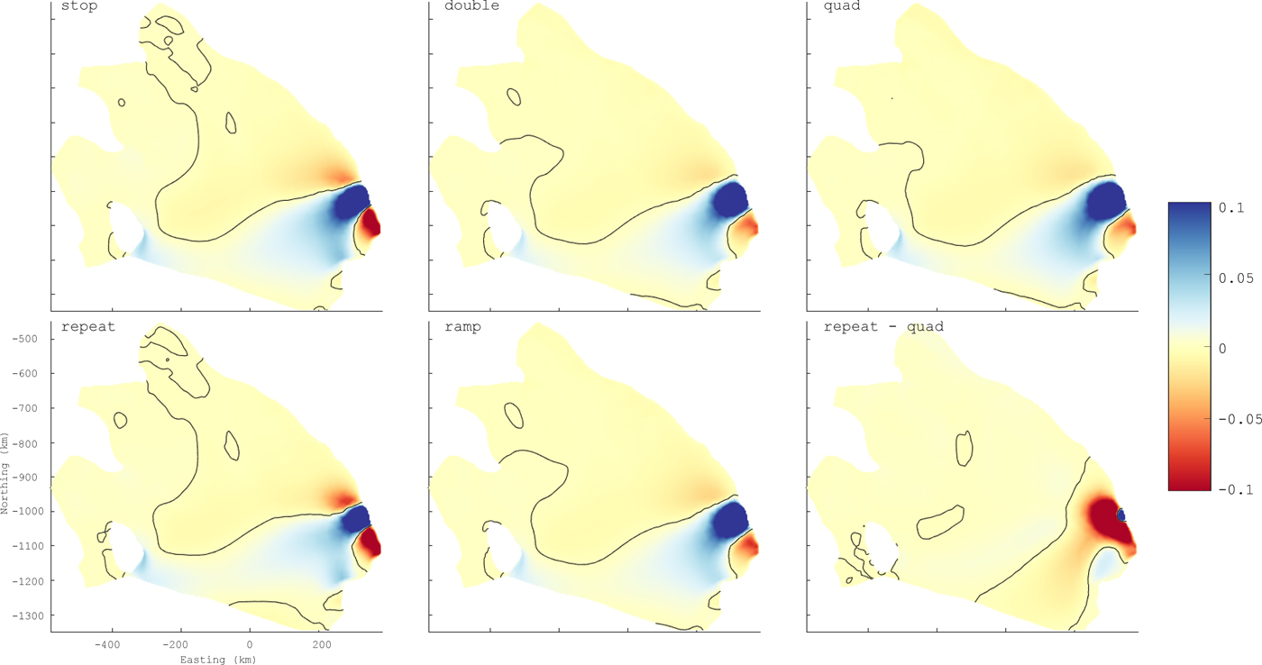
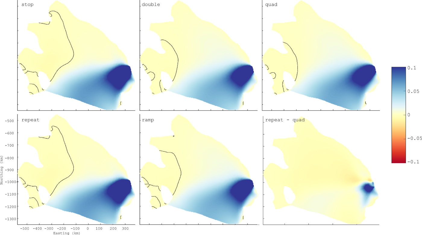
Here we present the leading response surface (first EOF) of the thickness transients ∂h/∂t and speed transients ∂u/∂t for each perturbation experiment (Figs 2 and 3). In the case of thickness, the leading response surfaces and their associated normalized eigenvalues, across all scenarios explain between 79 and 88% of the model data (Table 2). In the case of velocity, the leading response surfaces, and their associated normalized eigenvalues, explain over 99% of the model data in each case.
Response surface (first EOF) of thickness transient ∂h/∂t for each experiment. Response surfaces have been scaled such that the maximum amplitude is 1. Note the colorbar extends from −0.1 to +0.1 to emphasize smaller features.
Response surface (first EOF) of speed transient ∂u/∂t for each experiment. Response surfaces have been scaled such that the maximum amplitude is 1. Note the colorbar extends from −0.1 to +0.1 to emphasize smaller features.
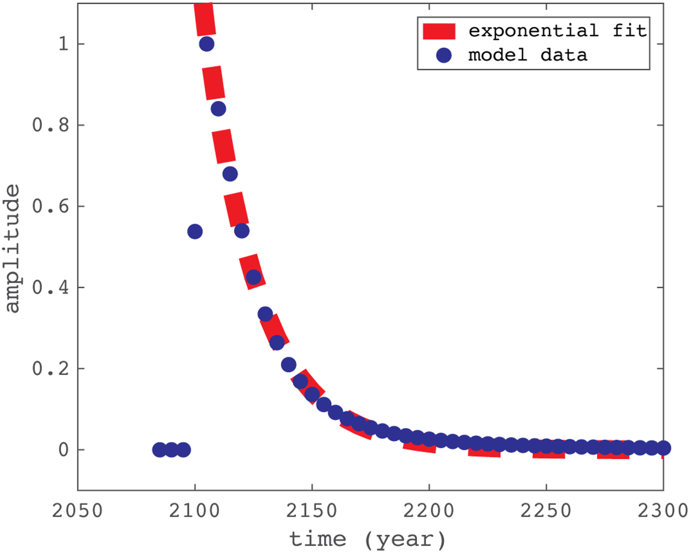
Response surface amplitude changes with time; they react instantaneously to the forcing and subsequently decay. These decays can be fit as exponential functions with associated response times (Fig. 4). We separate response times into speed-up and slowing response times.
The time series of the amplitude of leading response surface (first EOF) of thickness transient ∂h/∂t experiment can be fit to an exponential function. The fit for the ‘double’ is shown here as an example.
Speed-up (slowing) response times are the e-folding times of fitted exponentials associated with speed increases (decreases) to Byrd Glacier. Errors in reported response times represent the 95% confidence level of the exponential fit to model data (Table 2). The ‘repeat’ experiment has many speed-up and slowing down responses; response times presented represent an average of those times.
Thickness transient data
The ultimate objective of creating response surfaces from numerically-generated data is their application as a tool to search for the same patterns in observational data. Lee and others (Reference Lee, Seo, Han, Yu and Scambos2012) used 3-D tracking surface features observed in ICESat laser altimetry in a Lagrangian sense to infer thickness change in RIS. Lagrangian thickness changes are converted to Eulerian thickness changes (Fig. 5) by removing the advection of thickness-gradients of the ice shelf in hydrostatic equilibrium (Moholdt and others, Reference Moholdt, Padman and Fricker2014), using surface elevation data from Bedmap2 (Fretwell and others, Reference Fretwell2013) and surface velocity data from IPY-MEaSUREs program (Rignot and others, Reference Rignot, Mouginot and Scheuchl2011). Eulerian thickness changes are corrected for firn compaction using the method of Ligtenberg and others (Reference Ligtenberg, Helsen and van den Broeke2011). The change patterns over several different intervals shown in Fig. 5 reflect a combination of perturbations from various sources, together with measurement error.
Transient thickness change ∂h/∂t (m a−1) from IceSAT laser altimetry over various epochs. The patterns are the sum of boundary perturbations and noise in the measurement. The thickness change pattern downstream from the outlet of Byrd Glacier (BG) and near the northeast of Roosevelt Island (RI) are similar to the response surface shown in the ‘ramp’ experiment of Fig. 2. WIS, Whillans Ice Stream; KIS, Kamb Ice Stream; BIS, Bindschadler Ice Stream; Mac, MacAyeal Ice Stream.

DISCUSSION
Thickness transient response surfaces
The thickness transient response surfaces were similar across the experiments, independent of forcing magnitude, shape and duration (Fig. 2). Strong transverse gradients near the outlet of Byrd Glacier are a defining feature of the response surfaces. This pattern is a consequence of shearing at the lateral boundaries where the thick, fast flowing glacier enters the ice shelf. Flow enhancement thickened the ice and increased velocity immediately downstream of the boundary, which also increased shear strain rates at the sides of the glacier outlet. The increased shearing, in turn, thinned the laterally outboard ice. When flux declined, the pattern reversed. Shearing still caused thinning along the margins, but with a smaller magnitude.
The thickness transient response surfaces reveal long-distance connections in ice shelf response to the boundary perturbation. The response surface is positive near the outlet of Byrd Glacier along with a region along the northwest coastline of Roosevelt Island. These regions are isolated from one another yet long-distance adjustments to the coupled velocity and thickness mean that when discharge changes at Byrd Glacier, ice thickness along the northwest shore of Roosevelt Island responds. Without the EOF analysis, we might find a different explanation for thickness change there.
While a particular flux gate will generate a characteristic response surface regardless of perturbation magnitude, small differences did emerge (see ‘repeat – quad’ panel of Fig. 2). The outboard lateral zone of enhanced/reduced shear was narrower in experiments where the speed of Byrd Glacier was reduced to zero (‘stop’ and ‘repeat’), hereafter called ‘stopping experiments’.
Stopping experiments also produced a large gradient in ∂h/∂t across the outboard lateral zone, associated with stronger shearing. Since the magnitude and width of shearing differ in these cases, it might be possible to use this region to distinguish between these forcing types in observations. However, it would be important to accurately determine the width of the zone when comparing model response surfaces to observational datasets.
In every experiment the slowing response time was longer than the speed-up response time. This makes sense, as the driving stress depends on ice thickness. The difference between speed-up and slowing response times for individual experiments increases with the difference in forcing magnitude.
However, this does not lead to the conclusion that larger perturbations produce longer-lasting effects because that scaling is accounted for when the exponential decay curve is generated. Differences in response times may be due to the non-linearity of the flow law or transient grounding in some experiments. Further analysis of response times and additional perturbation experiments are required to determine the relative contribution of those two effects.
Speed transient response surfaces
Speed transient response surfaces were relatively uniform across our model scenarios (Fig. 3). The spatial patterns are relatively smooth and clearly show how much of the ice shelf is influenced by the velocity boundary condition imposed by Byrd Glacier. As with the thickness response surfaces, some modest differences are apparent (see ‘repeat - quad’ panel of Fig. 2). Stopping experiments generated an anomaly that extended across a larger reach of the ice shelf, encompassing several ice stream grounding zones.
The leading response surface (first EOF) explained more of the total variance in the velocity than in the ice thickness because changes in velocity boundary conditions generate an instantaneous change in ice flow. We note that while the change in boundary condition generates a change in thickness that itself drives additional change in the velocity, the effect was small in the case of the experiments presented here. Perturbations at other boundaries, in particular those leading to significant grounding or ungrounding, may have different outcomes.
Comparison with observations
Byrd Glacier accelerated by ~10% of its original speed between 2005 and 2007 in association with a subglacial water drainage event (Stearns and others, Reference Stearns, Smith and Hamilton2008). Because this perturbation was so recent, its effects should be discernible in observed thickness change. Our ‘ramp’ experiment is the most similar to the event and predicts strong transverse gradient in the thickness transient near the outlet of Byrd Glacier and a teleconnection with the northwest coast of Roosevelt Island (Fig. 2). All time intervals in our dataset involve the Byrd Glacier speed-up event and the observation duration is short compared with the e-folding time of Byrd perturbation. Therefore all intervals in our dataset contain a component that resembles our calculated response surface.
Indeed, many features of the Byrd response surface are visible in the data (Fig. 5). The strong transverse gradient is visible at all intervals, although it is imprinted on regional patterns of thickening. A teleconnection is visible between the outlet of Byrd Glacier and the the northwest coast of Roosevelt Island. The amplitude of this connection appears to decline over time, consistent with our model-derived response surface.
CONCLUSIONS
Here we set out to demonstrate the application of EOF analysis to identify characteristic patterns of change associated with a particular boundary perturbations and to understand how those patterns are affected by the magnitude, shape and duration of the perturbation. We accomplished this using a model of RIS with various adjustments to Byrd Glacier. We have three main conclusions. (1) Thickness and speed transient response surfaces associated with perturbations to Byrd Glacier appear to be independent of duration, magnitude and shape of the perturbation. (2) Timescales associated with thickness transient response surfaces depend on magnitude and sign of the perturbation. (3) There is evidence of a known Byrd Glacier event in recently observed thickness change on RIS.
The Byrd Glacier perturbation experiments performed here are a simple case study into a method that can be applied to more complicated scenarios and to extract information from contemporary observations of change. Boundary perturbations such as ice shelf calving, ice stream activation and grounding events could all be considered with this type of analysis. It will be possible to determine the shape of each these boundary perturbations and their associated durations. As the observational record extends, we expect that it will be possible to identify response surfaces that match those of boundary perturbations. This will let us be more confident as to which signals are definitively associated with internal variability and those for which an external cause must be found.
ACKNOWLEDGMENTS
We thank the University of Washington Glaciology Group and Ting Wang for their helpful discussions. We also thank Olga Sergienko and Helen Fricker for helpful comments and suggestions during the review process and an anonymous reviewer for a good time. This work has been funded by the NZARI 2014-11 grant, ‘Vulnerability of the Ross Ice Shelf in a Warming World.’


 Open access