


1. Introduction
Alternate migrating bars are large-scale bedforms common in wide, shallow alluvial rivers with a fairly uniform geometry. They are known to spontaneously form as the result of an instability of the erodible bed, which tend to amplify natural bed disturbances when the half-width-to-depth ratio,  $\beta$, is larger than a critical value $\beta _C$ (Callander Reference Callander1969; Parker Reference Parker1976; Fredsoe Reference Fredsoe1978; Colombini, Seminara & Tubino Reference Colombini, Seminara and Tubino1987; Nelson Reference Nelson1990; Bertagni, Perona & Camporeale Reference Bertagni, Perona and Camporeale2018). Linear theories allow for predicting their wavelength, scaling with the river width, while weakly nonlinear theories allow for predicting their amplitude, scaling with the river depth.
However, river bars can also be forced by geometrical variations associated with in-stream obstacles (Struiksma & Crosato Reference Struiksma and Crosato1989; Crosato et al. Reference Crosato, Mosselman, Beidmariam Desta and Uijttewaal2011; Siviglia et al. Reference Siviglia, Stecca, Vanzo, Zolezzi, Toro and Tubino2013), channel width variation (Repetto, Tubino & Paola Reference Repetto, Tubino and Paola2002; Wu, Shao & Chen Reference Wu, Shao and Chen2011; Duró, Crosato & Tassi Reference Duró, Crosato and Tassi2016), channel bifurcation (Bertoldi & Tubino Reference Bertoldi and Tubino2007; Redolfi, Zolezzi & Tubino Reference Redolfi, Zolezzi and Tubino2016; Le, Crosato & Uijttewaal Reference Le, Crosato and Uijttewaal2018; Salter, Voller & Paola Reference Salter, Voller and Paola2019) or curvature of river meanders (Blondeaux & Seminara Reference Blondeaux and Seminara1985; Struiksma et al. Reference Struiksma, Olesen, Flokstra and De Vriend1985; Zolezzi et al. Reference Zolezzi, Guala, Termini and Seminara2005). Forced alternate bars, which are most common in nature, are steady (non-migrating) and tend to decay in space. A typical configuration of forced bars is the point bar forming along the inner curve of meandering rivers. Because the forced bar is steady, it imposes a specific distribution of shear stress along the erodible bed and streambanks, which defines preferential regions of localized erosion eventually controlling the planform evolution of meanders (Ikeda, Parker & Sawai Reference Ikeda, Parker and Sawai1981; Seminara & Tubino Reference Seminara and Tubino1992; Parker et al. Reference Parker, Shimizu, Wilkerson, Eke, Abad, Lauer, Paola, Dietrich and Voller2011).
A crucial parameter associated with forced bars (Seminara Reference Seminara2010) is the resonant aspect ratio  $\beta _R$, originally defined by Blondeaux & Seminara (Reference Blondeaux and Seminara1985), which controls the direction of the morphodynamic influence with respect to the external forcing. Zolezzi & Seminara (Reference Zolezzi and Seminara2001) showed analytically that steady alternate bars can form upstream or downstream of a channel curvature discontinuity depending on whether $\beta$ is larger (super-resonant) or smaller (sub-resonant) than the resonant value, respectively. Experimental findings and theoretical considerations (e.g. Struiksma & Crosato Reference Struiksma and Crosato1989; Zolezzi et al. Reference Zolezzi, Guala, Termini and Seminara2005; Crosato et al. Reference Crosato, Mosselman, Beidmariam Desta and Uijttewaal2011; Siviglia et al. Reference Siviglia, Stecca, Vanzo, Zolezzi, Toro and Tubino2013) reveal that any permanent, localized distortion of the cross-section can potentially trigger the non-local formation of forced bars in a straight channel. This suggests that the formation of forced bars could be more common than expected and potentially associated with a broad class of finite, but spatially impulsive, perturbations. Moreover, it also suggests that some form of control of the spatial evolution of river bathymetries is possible.
Recent experimental investigations on the interaction between current energy converters (known as CEC), more commonly known as marine hydrokinetic (MHK) turbines, and the surrounding river environment, revealed that asymmetric deployments of in-stream hydrokinetic turbines can trigger large-scale, river bed deformations. Specifically, Musa et al. (Reference Musa, Hill, Sotiropoulos and Guala2018b) and Musa, Hill & Guala (Reference Musa, Hill and Guala2019) showed that asymmetric installation of hydrokinetic turbines induce an average topography distortion that resembles the characteristic features of forced, steady, alternate bars. Hydrokinetic turbines harness the kinetic energy of natural flows such as tides and rivers, to generate renewable energy. They represent an early stage technology which could be deployed more broadly in natural or channelized systems, provided we know their feedback effects on the flow and on both local and non-local erosional–depositional processes. However, as highlighted by Musa et al. (Reference Musa, Hill and Guala2019) the relationship between the external forcing (i.e. the turbines) and the observed morphodynamic effect is far from being clear. Specifically, experiments suggest that although the shear stress and the blockage ratios are relevant quantities for the amplification of non-local effects, other parameters must be considered as well. For instance, the aspect ratio  $\beta$ and the corresponding resonant condition $\beta _R$, controlling the onset of forced alternate bars, were deemed to be critically important to amplify or dampen the induced local bathymetric effects.
According to the linear theories (e.g. Struiksma et al. Reference Struiksma, Olesen, Flokstra and De Vriend1985; Zolezzi & Seminara Reference Zolezzi and Seminara2001), the wavelength and the spatial extension of the forced bar pattern should not depend on the specific nature of the forcing, albeit only on the channel conditions in terms of  $\beta$ as compared with its resonant value $\beta _R$, Shields stress and relative roughness. Considering the experimental results collected on non-local effects induced by MHK turbines (in this case the forcing or external stressor), two main questions emerged. (i) Can we assume that the mean bed oscillations observed in Musa et al. (Reference Musa, Hill, Sotiropoulos and Guala2018b, Reference Musa, Hill and Guala2019) are a bar-type phenomenon? (ii) How do the characteristics of the forcing influence the resulting mean bed distortion? In order to answer these questions, we hypothesize in this contribution that the bar forcing effect is induced by the asymmetric drag force exerted by the obstacle along the cross-section. Our formulation is based on the linearized, two-dimensional (2-D), depth-averaged shallow water model of Zolezzi & Seminara (Reference Zolezzi and Seminara2001). The model is here coupled with a novel internal boundary condition that accounts for the presence of a localized, asymmetrical drag force, as needed to represent the non-local effect exerted by hydrokinetic turbines, vegetation patches, and in general by any permeable perturbation that covers a limited portion of the cross-section.
To bridge the gap between the model assumptions and the experimental results with hydrokinetic turbines, we performed a second set of experiments where the finite perturbations are enacted by a porous grid covering a well-defined portion of the cross-section and consistent with the boundary conditions imposed in the formulation.
The choice of a porous, permeable grid as an obstacle is based on the implementation and validation of porous disk actuator models for wind turbines, which were able to capture the essential features of turbine wakes (Sørensen Reference Sørensen2011). Another advantage of a porous grid, asymmetrically installed on one half of the channel, is that it represents a hydrodynamic perturbation similar to the dual MHK turbines studied in Musa et al. (Reference Musa, Hill and Guala2019), but without the depth constrains. This allows us to test a broader range of  $\beta$-values and, more interestingly, to move towards resonant conditions. The primary goal is to reproduce experimentally and theoretically the non-local oscillations in the mean bed that were observed under intense sediment transport and under an asymmetric distribution of the drag force (i.e. an asymmetric deployment of turbines or porous grids). The secondary goal is to explore the parameter space through a validated predictive model able to quantify non-local scour–deposition processes associated with different finite perturbations, channel geometry and sediment transport conditions.
In §§ 2 and 3 we describe our theoretical approach, our dimensionless variable space and the basic equations embedded in the model. Section 4 is focused on the experimental apparatus, including the measurements of the drag force induced by the grid. Experimental and numerical results are compared in § 5. Discussion and conclusions follow.
2. Formulation of the problem
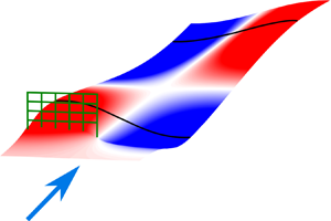
To model the effect of the obstacle on the erodible bed, we consider an infinitely long channel with straight and fixed banks and rectangular cross-section of width  $2B^*$ (figure 1a), whose bottom is formed by well-sorted, cohesionless particles with median grain size $ds^*$, with the star superscript denoting dimensional quantities. The origin of the Cartesian system of reference ( $x^*,y^*$) is positioned at the right-hand bank, while the porous grid of width $\delta ^*$ is located near the left-hand bank at $x^*=0$.
Geometrical configuration and notation: (a) planimetric view; (b) cross-sectional view (from upstream), where  $F^*$ indicates the force exerted by the grid on the fluid. The dashed line indicates the internal boundary that separates the two, semi-infinite domains (channel A and channel B).

We adopt a 2-D, mobile-bed, depth-averaged shallow water model (i.e. Colombini et al. Reference Colombini, Seminara and Tubino1987; Crosato et al. Reference Crosato, Mosselman, Beidmariam Desta and Uijttewaal2011; Siviglia et al. Reference Siviglia, Stecca, Vanzo, Zolezzi, Toro and Tubino2013), which can be written as a nonlinear differential system of four equations in the four dependent variables  $\eta ^*$, $U^*$, $V^*$, $D^*$ (bottom elevation, longitudinal and transverse velocity and water depth, respectively, see figure 1b) in the two independent variables $x^*,y^*$.
The four dependent variables are made dimensionless as
 \begin{equation} \{U,V\}=\frac{\{U^*,V^*\}}{U_0^*},\quad D=\frac{D^*}{D_0^*},\quad \eta=\frac{\eta^*}{D_0^*}, \end{equation}
where  $D_0^*$ and $U_0^*$ are the reference values of depth and longitudinal velocity, which are defined as the uniform flow values that are expected when the channel is undisturbed (i.e. no obstacle). Similarly, the grain size is made dimensionless as
 \begin{equation} ds_0=\frac{ds^*}{D_0^*}. \end{equation}
 Planimetric coordinates and grid width are scaled with half the channel width  $B^*$ as
 \begin{equation} x=\frac{x^*}{B^*},\quad y=\frac{y^*}{B^*},\quad \delta=\frac{\delta^*}{B^*}, \end{equation}
so that both  $\delta$ and $y$ range from $0$ to $2$.
$2$.
Similarly, the components of the stress vector and the unit bedload vector are made dimensionless as follows:
 \begin{equation} \{\tau_x,\tau_y\}=\frac{\{\tau_x^*,\tau_y^*\}}{\rho U_0^{*2}},\quad \{qs_x,qs_y\}=\frac{\{qs_x^*,qs_y^*\}}{\sqrt{g{\rm \Delta} ds^{*3}}}, \end{equation}
where  $g$,
$g$,  $\rho$ and ${\rm \Delta}$ indicate the gravitational acceleration, the water density and the relative submerged density of the bed material, respectively.
Finally, the drag force exerted on the grid is scaled as
 \begin{equation} f=\frac{f^*}{\rho U_0^{*2} D_0^*}, \end{equation}
where  $f^*=F^*/\delta ^*$ is the drag force per unit width.
The depth-averaged equations that express the conservation of momentum, liquid and solid mass can be written in dimensionless form as
 \begin{gather} U\frac{\partial U}{\partial x} + V\frac{\partial U}{\partial y} + \frac{1}{Fr_0^2}\frac{\partial H}{\partial{x}} +\beta_0\frac{\tau_{x}}{D} = 0, \end{gather}
 \begin{gather}U\frac{\partial V}{\partial x }+ V\frac{\partial V}{\partial y} + \frac{1}{Fr_0^2}\frac{\partial H}{\partial y} + \beta_0\frac{\tau_{y}}{D} = 0, \end{gather}
 \begin{gather}\frac{\partial UD}{\partial x} + \frac{\partial VD}{\partial y} = 0, \end{gather}
 \begin{gather}\frac{\partial qs_{x}}{\partial x}+ \frac{\partial qs_y}{\partial y} = 0, \end{gather}
where the reference Froude number and aspect ratio are given by
 \begin{equation} Fr_0=\frac{U_0^*}{\sqrt{gD_0^*}},\quad \beta_0=\frac{B^*}{D_0^*} \end{equation}
and  $H=\eta +D$ indicates the dimensionless water surface elevation (WSE) scaled with $D_0^*$.
The solution of the system of partial differential equations (2.6a) needs closure relations for the quantities  $\tau _x$, $\tau _y$, $qs_x$, $qs_y$. The shear stress vector is assumed to point in the opposite direction to the velocity vector, and its magnitude is computed by means of the Chézy formula,
 \begin{equation} |\boldsymbol{\tau}|=\frac{U^2+V^2}{c^2}. \end{equation}
 Variations of the Chézy coefficient  $c$ with water depth can be estimated through of the following logarithmic expression (Keulegan Reference Keulegan1938):
 \begin{equation} c=6+2.5\log\left(\frac{D}{k_s}\right),\quad k_s=k_s^*/D_0^*, \end{equation}
where  $k_s^*$ is a roughness length that also accounts for the presence of bedforms. When applied to the reference flow, (2.9a,b) reads
 \begin{equation} c_0=6+2.5\log\left(\frac{1}{k_s}\right). \end{equation}
Equation (2.10) provides a simple relation between  $k_s$ and the reference Chézy parameter $c_0$ that can be calculated as
 \begin{equation} c_0=U_0^*/u_*, \end{equation}
where the shear velocity  $u_*$ is obtained from experimental measurements in presence of migrating dunes.
To quantify the sediment transport rate, we must consider that only a portion of the shear stress contributes to transport sediments, suggesting the separation of the so-called (bed)form drag from the skin friction drag (Einstein Reference Einstein1950) the latter being expressed as
 \begin{equation} |\boldsymbol{\tau_s}|=\frac{U^2+V^2}{c_s^2}. \end{equation}
The component of the dimensionless Chézy coefficient due to the skin drag,  $c_s$ can be calculated as (e.g. Engelund & Fredsoe Reference Engelund and Fredsoe1982; Toyama et al. Reference Toyama, Shimizu, Yamaguchi and Giri2007)
 \begin{equation} c_s=6+2.5\log\left(\frac{D_s}{2.5ds_0}\right), \end{equation}
where  $D_s$ represents the component of the flow depth due to the skin friction alone. The magnitude of the solid discharge is then expressed as a function of the skin Shields number $\theta _s$, namely
 \begin{equation} |\boldsymbol{qs}|^*=\varPhi(\theta_s)\sqrt{g{\rm \Delta} ds^{*3}},\quad \theta_s=\frac{|\boldsymbol{\tau_s}|^*}{\rho g {\rm \Delta} ds^*}=Fr_0^2\frac{|\boldsymbol{\tau_s}|}{{\rm \Delta} ds_0}. \end{equation}
The function  $\varPhi (\theta _s)$ can be estimated by means of the widely used bedload formula of Meyer-Peter & Muller (Reference Meyer-Peter and Muller1948),
 \begin{equation} \varPhi=8 \left(\theta_s-\theta_{cr}\right)^{1.5},\quad \theta_{cr}=0.047, \end{equation}
where  $\theta _{cr}$ indicates the critical Shields number for incipient sediment transport. Finally, the direction of the bedload can be calculated (Ikeda Reference Ikeda1982; Baar et al. Reference Baar, de Smit, Uijttewaal and Kleinhans2018) as a sum of two angles: the one formed by the velocity vector (with respect to the $x$-axis) and the correction due to the bottom gradient in the transverse direction, namely
 \begin{equation} \tan(\gamma_q)=\left(\frac{V}{U}\right),\quad \tan(\gamma_g)={-}\frac{r}{\beta_0\sqrt{\theta_s}}\frac{\partial \eta}{\partial y}, \end{equation}
where  $r$ is an empirical parameter ranging from $0.3$ to $0.6$, with $r=0.5$ representing a typical choice in morphodynamic models.
Once the four closure relations are specified, we can complete the mathematical formulation by specifying the boundary conditions, which derive from considering impermeable banks,
 \begin{equation} qs_y(x,0)=qs_y(x,2)=0,\quad V (x,0)=V(x,2)=0. \end{equation}
For more details about the formulation, see Colombini et al. (Reference Colombini, Seminara and Tubino1987) and Zolezzi & Seminara (Reference Zolezzi and Seminara2001).
3. The perturbation approach
The analytical solution is derived using a linear perturbation approach (e.g. Repetto et al. Reference Repetto, Tubino and Paola2002). For an undisturbed (i.e.  $f=0$) channel, the solution of the system (2.6a) is simply a uniform flow, with the bed having a constant longitudinal slope $S_0$, as follows:
 \begin{equation} \eta_0={-}S_0 \beta_0x, \end{equation}
and with unitary values of dimensionless water depth and longitudinal velocity. This solution is used as a reference state for expanding the general solution in Taylor series in the parameter  $f$:
$f$:
 \begin{equation}
\left\{\eta,U,V,D
\right\}=\underbrace{\left\{\eta_0(x),1,0,1 \right\}
}_{\substack{\text{reference solution} \\ \text{(uniform
flow)} }}
+\underbrace{f\left\{\eta_1,U_1,V_1,D_1\right\}(x,y)}_{
\substack{\text{first-order (linear)} \\
\text{approximation} }} +\underbrace{O(\,f^2) }_{
\substack{\text{higher-order (nonlinear)}\\ \text{terms}
}},
\end{equation}
\begin{equation}
\left\{\eta,U,V,D
\right\}=\underbrace{\left\{\eta_0(x),1,0,1 \right\}
}_{\substack{\text{reference solution} \\ \text{(uniform
flow)} }}
+\underbrace{f\left\{\eta_1,U_1,V_1,D_1\right\}(x,y)}_{
\substack{\text{first-order (linear)} \\
\text{approximation} }} +\underbrace{O(\,f^2) }_{
\substack{\text{higher-order (nonlinear)}\\ \text{terms}
}},
\end{equation}
where the subscripts  $0$ and $1$ indicate the reference solution and the first-order approximation, respectively.
If we assume that the drag force is relatively small with respect to the momentum carried by the flow, we can expect that all the perturbations with respect to the reference solution are also small. This allows us to neglect the higher-order terms in the asymptotic expansion, so that (3.2) becomes linear in the parameter  $f$. Equation (3.2) can be substituted in the system (2.6a) and in the closure relations, which in turn can be expanded in Taylor series. Neglecting the higher-order terms will then give a system of four linear equations with four unknowns $\{\eta _1,U_1,V_1,D_1\}$.
The procedure we adopted to obtain the solution of the linear system for our specific problem is based on three main steps. First, we split the domain in two separate regions (see figure 1a): the upstream channel A ( $x=(-\infty ,0]$) and the downstream channel B ( $x=[0,+\infty )$). Second, we seek a general solution for the two semi-infinite channels, which can be obtained by expressing the solution as a linear superposition of 2-D Fourier modes (see Zolezzi & Seminara Reference Zolezzi and Seminara2001). Third, we add the effect of the localized momentum sink produced by the grid by imposing proper matching conditions at the internal boundary (i.e. at $x=0$). As detailed below, this procedure allows for obtaining a unique solution expressed as a Fourier series.
3.1. The linear solution for the individual channels A and B
A general solution of the steady, linear problem for a straight channel can be readily obtained by separating the variables and decomposing the transverse structure of the solution in Fourier modes (see Zolezzi & Seminara Reference Zolezzi and Seminara2001). Specifically, for each transverse Fourier mode  $m$ it is possible to find a solution as a sum of four complex exponentials in $x$, namely
 \begin{gather} \{\eta_1,U_1,D_{1}\} =\cos(m{\rm \pi} y/2)\sum_{j=1}^4\tilde{\eta}_{mj}\{1,u_{mj},d_{mj}\} \exp(\lambda_{mj}x) \quad m\ge 1, \end{gather}
 \begin{gather}V_1=\sin(m{\rm \pi} y/2)\sum_{j=1}^4\tilde{\eta}_{mj}{v}_{mj}\exp(\lambda_{mj}x)\quad m\ge 1, \end{gather}
where, despite the results being complex numbers, only the real part is physically significant.
In (3.3),  $\tilde {\eta }_{mj}$ are independent parameters, while the coefficients $\{u_{mj},v_{mj},d_{mj}\}$ and the wavenumbers $\lambda _{mj}$, exclusively depend on the basic reference flow. Specifically, the wavenumbers $\lambda _{mj}$ can be computed by solving the fourth-order polynomial that represents the dispersion relation, and the sign of their real part, $(\lambda _{mj})_R$, is fundamental in defining the spatial structure of the solution.
This can be explained by noticing that for semi-infinite channels, not all the four components of the solution (3.3) can be considered to build the general solution. Let us consider for example the downstream channel B: components having positive eigenvalues (i.e.  $(\lambda _{mj})_R>0$) are exponentially growing in $x$, so that they are determined by the downstream boundary condition (see (6.6) of Zolezzi & Seminara (Reference Zolezzi and Seminara2001)). If the channel is sufficiently long, this boundary condition does not affect the bed distortion, and the contribution of the positive eigenvalue vanishes. Similarly, components of the solution for channel A that show negative eigenvalues $(\lambda _{mj})_R<0$ (i.e. exponentially growing in the upstream direction) are determined by the upstream conditions, and are therefore identically vanishing when the channel is infinitely long.
For the modes  $m>1$ the dispersion relation always gives three positive and one negative eigenvalue (except for extremely wide and shallow channels, having $\beta _0\ge 2\beta _R$). Conversely, for the fundamental mode $m=1$ the sign of $(\lambda _{mj})_R$ varies with the aspect ratio as illustrated in figure 2(a): when $\beta _0<\beta _R$ (sub-resonant conditions) three eigenvalues are negative (i.e. compatible with the channel B) and one is positive (i.e. compatible with the channel A), while the opposite occurs when $\beta _0>\beta _R$ (super-resonant conditions).
(a) Real part of the eigenvalues  $\lambda _{1j}$, representing the spatial growth/damping rate of first Fourier mode ( $m=1$) as a function the channel aspect ratio $\beta _0$, here illustrated in logarithmic scale to highlight the quasisymmetry with respect to the resonant aspect ratio $\beta _R$. (b) List of compatible eigenvalues for the upstream ( $\,j^A$) and the downstream ( $\,j^B$) channel for different Fourier modes ( $m$), depending on the channel being under sub-resonant or super-resonant conditions. Adapted from figures 3 and 4 of Redolfi et al. (Reference Redolfi, Zolezzi and Tubino2016).

Consequently, the list of compatible eigenvalues depends on channel conditions as summarized in figure 2(b). As first highlighted by Zolezzi & Seminara (Reference Zolezzi and Seminara2001), the distinction between sub-resonant and super-resonant regimes has a great importance. The eigenvalues  $j=\{2,3\}$, being the smallest in terms of absolute value of the real part, represent a component of the solution that slowly decays in space. Therefore, depending on whether they fall in the upstream or in the downstream channel defines the dominant direction of the morphodynamic influence.
For a more comprehensive description of the phenomena, see Zolezzi & Seminara (Reference Zolezzi and Seminara2001) and Redolfi et al. (Reference Redolfi, Zolezzi and Tubino2016).
3.2. The matching conditions at the internal boundary
The solution for the individual, semi-infinite channels of (3.3) is mathematically underdetermined, as all the coefficients  $\tilde {\eta }$ can assume any arbitrary value. To determine the coefficients, we need to specify appropriate boundary conditions. In particular, we need to set four matching conditions at the internal boundary. Each condition is specified along the entire cross-section at $x=0$; therefore, it cannot be simply represented by a scalar value, but as a function of the transverse coordinate $y$. However, when expanded in Fourier series, each function reduces to a scalar condition for each Fourier mode.
The first two conditions are simply defined by the water and sediment continuity. The third relation is derived assuming the conservation of the transverse momentum (i.e. no significant transverse force exerted by the grid), which implies no jumps of the transverse velocity across the grid. The above internal boundary conditions can be summarized as follows:
 \begin{gather} U_1^A+D_1^A=U_1^B+D_1^B, \end{gather}
 \begin{gather}2\varPhi_T[ U_1^A-c_D D_1^A]=2\varPhi_T[U_1^B-c_D D_1^B], \end{gather}
 \begin{gather}V_1^A=V_1^B, \end{gather}
where each variable is evaluated at  $x=0$, thus consisting of a function of the transverse coordinate $y$ only. The coefficients, $c_D$ and $\varPhi _T$ measure the sensitivity of the Chézy coefficient and the sediment transport to variations of depth and Shear stress, and can be easily calculated from (2.9a,b) and (2.15a,b), which give the following expressions:
 \begin{equation} c_D:=\left.\frac{D_0}{C_0}\frac{\partial c}{\partial D}\right|_{D=D_0} = \frac{2.5}{c_0},\quad \varPhi_T:=\frac{\theta_{0s}}{\varPhi_0} \left.\frac{\partial \varPhi}{\partial \theta_s}\right|_{\theta_s = \theta_{0s}}=1.5 \frac{\theta_{0s}}{\theta_{0s}-\theta_{cr}}. \end{equation}
By combining terms of (3.4) we obtain a rather simple set of matching conditions,
 \begin{gather} U_1^A(0,y)=U_1^B(0,y), \end{gather}
 \begin{gather}D_1^A(0,y)=D_1^B(0,y), \end{gather}
 \begin{gather}V_1^A(0,y)=V_1^B(0,y), \end{gather}
which shows that water depth and both velocity components are conserved across the grid. It is worth noticing that the above result is characteristic of an equilibrium mobile bed solution, resulting from an adaptation of the bed until the upstream and downstream sediment transport capacities are equal. This is not the case in fixed bed conditions, where in general the upstream depth and velocity differ from their downstream counterparts (see appendix A).
As anticipated, we then need to specify a fourth condition, which is the key to incorporate the effect of the drag force in the present model. In mobile bed conditions we cannot simply assume that the bottom is flat, but we need to consider the possible formation of an elevation difference near the grid, which can be modelled as a localized bottom step. There are essentially two ways to obtain the same expression for this elevation difference.
The first approach is based on a direct application of the momentum conservation across the grid (see figure 3). In steady flow conditions, the momentum balance (per unit width) can be expressed as
 \begin{equation} s^{*A}+s^{*S}=s^{*B} + f^* I(y), \end{equation}
where  $s^*$ indicates the force per unit width, and $I$ is a 0–1 indicator function which vanishes outside the grid. Considering the grid positioning illustrated in figure 1, $I(y)$ is simply a (shifted) Heaviside function, namely
 \begin{equation} I(y)=\begin{cases} 1 & y>(2-\delta) \\ 0 & \textrm{elsewhere} \end{cases}. \end{equation}
Definition of the control volume (shaded area) used to apply the momentum balance across the grid, with  $f^*$, $s^{*A}$, $s^{*B}$ and $s^{*S}$ indicating the forces (per unit width) exerted by the grid, the upstream and downstream flow and the bottom step, respectively.

Since the upstream and the downstream flow have the same depth and velocity, they also carry the same momentum (i.e.  $s^{*A}=s^{*B}$). Consequently, the momentum balance (3.7) reduces to
 \begin{equation} s^{*S}=f^* I(y). \end{equation}
 It is therefore crucial to evaluate  $s^{*S}$, namely the longitudinal force exerted by the potential bottom step. This force can be modelled by assuming a hydrostatic distribution over the step (Fraccarollo & Capart Reference Fraccarollo and Capart2002), calculated using the average between the upstream and the downstream depth as follows:
 \begin{equation} s^{*S}=\underbrace{\rho g \frac{D^{*A}+D^{*B}}{2}}_{\text{hydrostatic pressure}} \underbrace{(\eta^{*A}-\eta^{*B})}_{\text{step height}}. \end{equation}
Equating (3.9) and (3.10) and expressing the result in dimensionless form, gives
 \begin{equation} \frac{1}{Fr_0^2}\frac{D^A+D^B}{2}(\eta^A-\eta^B)=f I(y), \end{equation}
which, by neglecting the higher-order terms in the Taylor expansion (3.2), gives
 \begin{equation} \eta_1^A-\eta_1^B=Fr_0^2 I(y), \end{equation}
which indicates that the bed elevation gap is proportional to the intensity of the forcing effect  $f$. It is worth noticing that the result of (3.12) would be the same if the hydrostatic pressure on the step was evaluated using either the upstream or the downstream depth instead of the mean, which makes this choice irrelevant for the linear analysis.
The second approach is based on the energy balance, which can be written in the following dimensionless form:
 \begin{equation} \eta_1^A+D_1^A+Fr_0^2U_1^A=\eta_1^B+D_1^B+Fr_0^2U_1^B+{\rm \Delta} e/f, \end{equation}
where  ${\rm \Delta} e$ indicates the loss of specific energy. Considering (3.6) the energy balance becomes
 \begin{equation} \eta_1^A=\eta_1^B+{\rm \Delta} e/f. \end{equation}
As detailed in appendix A, the energy loss induced by the grid can be estimated as
 \begin{equation} {\rm \Delta} e/f=I(y)Fr_0^2, \end{equation}
which leads to exactly the same result as in (3.12).
Summarizing, the set of four matching conditions given by (3.6) and (3.12) reads
 \begin{gather} \eta_1^A\left(0,y\right)=\eta_1^B\left(0,y\right) + Fr_0^2\ I(y), \end{gather}
 \begin{gather}U_1^A\left(0,y\right)=U_1^B\left(0,y\right), \end{gather}
 \begin{gather}V_1^A\left(0,y\right)=V_1^B\left(0,y\right), \end{gather}
 \begin{gather}D_1^A\left(0,y\right)=D_1^B\left(0,y\right), \end{gather}
where all the primary variables are conserved except for the bed elevation, which exhibits a step that is proportional to the drag force per unit width  $f$. It is important to note that the internal boundary condition represents the main theoretical contribution of this work that enables the extension of the morphodynamic influence framework of Zolezzi & Seminara (Reference Zolezzi and Seminara2001) to generic alterations of the cross-section as a function of its geometrical and drag properties.
All the terms of (3.16), except for  $I(y)$, are represented as a Fourier series in the transverse direction $y$. To obtain a separate solution for the individual Fourier modes, we need to expand also the indicator function, which gives
 \begin{equation} I(y)=\sum_{m=0}^{\infty} \hat{A}_m \cos({\rm \pi} y/2), \end{equation}
whose coefficients can be calculated as
 \begin{equation}
\hat{A}_m=\begin{cases} \dfrac{\delta}{2} & m=0 \\
-\dfrac{2}{m{\rm \pi}}\sin[m{\rm \pi}(1-\delta)/2] & m\ge
1 \end{cases}.
\end{equation}
\begin{equation}
\hat{A}_m=\begin{cases} \dfrac{\delta}{2} & m=0 \\
-\dfrac{2}{m{\rm \pi}}\sin[m{\rm \pi}(1-\delta)/2] & m\ge
1 \end{cases}.
\end{equation}
In practice, the series needs to be truncated to a number of Fourier modes  $N$, which provides the approximated distribution of $I(y)$ that is illustrated in figure 4(a). For the analysis of the model results and the comparison with laboratory experiments, $N=10$ modes were deemed to be sufficient to accurately represent the effect of the drag force distribution on the channel morphology.
Fourier series expansion of the indicator function that specifies the transverse distribution of the drag force (3.17). (a) Fourier representation depending on the number of modes  $N$ (example with grid size $\delta =0.6$). (b) Amplitude the Fourier coefficients (3.18) depending on $\delta$: the dotted line indicates the one-dimensional (1-D) component of the expansion; the dashed lines refer to the odd modes; the solid lines indicate the even modes, which vanish when the obstruction occupies half of the channel width (i.e. at $\delta =1$).

3.3. The 1-D component of the solution
The 1-D component of the steady solution gives unperturbed depth, longitudinal velocity and bed slope, but a difference in bed elevation across the grid. This elevation drop is simply proportional to the  $\hat {A}_0$ component of the Fourier expansion (dashed line of figure 4), namely
 \begin{equation} \eta_0^B=\eta_0^A+\hat{A}_0, \end{equation}
and is associated with an equal gap in the free surface elevation.
In subcritical (i.e.  $Fr_0<1$) conditions, the elevation difference $\hat {A}_0$ is expected to develop as a deposition in the upstream channel, where the flow tends to slow down due to the presence of the grid. This deposition front gradually propagates in the upstream direction, until the solution eventually attains uniform-slope conditions.
3.4. The 2-D component of the solution
Expressing the solution in the form of (3.3) for both channel A and channel B, and substituting into the four matching conditions (3.16) gives a set of relationships for the coefficients  $\tilde {\eta }$ as follows:
 \begin{equation} \left.\begin{gathered}
\sum_{j\in j^A}\tilde{\eta}_{mj}^A =\sum_{j\in
j^B}\tilde{\eta}_{mj}^B + Fr_0^2 \hat{A}_m \\ \sum_{j\in
j^A}\tilde{\eta}_{mj}^A u_{mj}=\sum_{j\in
j^B}\tilde{\eta}_{mj}^B u_{mj} \\ \sum_{j\in
j^A}\tilde{\eta}_{mj}^A v_{mj}=\sum_{j\in
j^B}\tilde{\eta}_{mj}^B v_{mj} \\ \sum_{j\in
j^A}\tilde{\eta}_{mj}^A d_{mj}=\sum_{j\in
j^B}\tilde{\eta}_{mj}^B d_{mj} \\
\end{gathered}\right\}\quad \forall\ m>0, \end{equation}
\begin{equation} \left.\begin{gathered}
\sum_{j\in j^A}\tilde{\eta}_{mj}^A =\sum_{j\in
j^B}\tilde{\eta}_{mj}^B + Fr_0^2 \hat{A}_m \\ \sum_{j\in
j^A}\tilde{\eta}_{mj}^A u_{mj}=\sum_{j\in
j^B}\tilde{\eta}_{mj}^B u_{mj} \\ \sum_{j\in
j^A}\tilde{\eta}_{mj}^A v_{mj}=\sum_{j\in
j^B}\tilde{\eta}_{mj}^B v_{mj} \\ \sum_{j\in
j^A}\tilde{\eta}_{mj}^A d_{mj}=\sum_{j\in
j^B}\tilde{\eta}_{mj}^B d_{mj} \\
\end{gathered}\right\}\quad \forall\ m>0, \end{equation}
which provides a set of  $4m$ equations for the $4m$ unknowns $\tilde {\eta }_{mj}^A$ ( $\,j\in j^A$), $\tilde {\eta }_{mj}^B$ ( $\,j\in j^B$).
The linear system (3.20) can be solved for each Fourier mode  $m$ independently, providing the values of the coefficients $\tilde {\eta }$. This allows us to uniquely determine the solution for the four dependent variables expressed by (3.3).
4. Experimental set-up
The experiments were carried out in the Tilting Bed Flume facility at St. Anthony Falls Laboratory at the University of Minnesota. The open channel flume is  $15\ \textrm {m}$ long, $0.9\ \textrm {m}$ wide and has slope adjustment capability that ranges from $-$1 % to 6 %. In our runs, the slope was set to approximately 0.15 %. The water discharge $Q^*$ is drawn directly from the adjacent Mississippi River and it is controlled by a calibrated actuating valve. The flow enters the channel through a 0.1 m long cobble stone wall and two rows of vertical cylinders of 0.05 m diameter and 0.05 m spacing, to break up large-scale turbulent structures. The channel is filled with a 0.2 m thick layer of coarse quartz sand with median grain $ds^*=1.25\ \textrm {mm}$. A sediment recirculation system ensures continuous sediment supply, which allows for maintaining the longitudinal bed slope in equilibrium.
A porous grid of width  $\delta ^*=0.45\ \textrm {m}$ was placed 6.4 m from the inlet, asymmetrically within the cross-section, and spanning half of the channel width (see figure 5). The height of the grid varied for different cases; except for G-H05 where the wall was set at mid-depth, the grid always extended above the water surface (see table 1). The grid is a stainless steel woven wire cloth, with a wire diameter of $d_{w}^*=0.002\ \textrm {m}$ and an opening size of $d_{o}^*=0.01\ \textrm {m}$. A mesh specific drag coefficient of $c_d=0.33$ was estimated towing the grid at constant speed through quiescent water, and measuring the resulting horizontal force (see top right-hand insert in figure 5 and the supplementary information in Musa et al. (Reference Musa, Hill, Sotiropoulos and Guala2018b)), and was used to estimate the drag force $F^*$ that is reported in table 1. The drag coefficient was observed to be Reynolds independent within the measured range ( $Re_h = 0.5 - 2 \times 10^5$, where $Re_h$ is referred to the grid height).
Experimental set-up for tests with porous grid. Dashed lines represent the streamwise transects scanned by the submerged sonar: the red line refers to the drag side (DS) (i.e. the half-channel obstructed by the grid), the blue line refers to the unobstructed side (US); both transects are located at the centre of the half-channel. The mesh is a stainless steel woven wire cloth, with a total width spanning half-channel  $\delta ^*=B^*=0.45\ \textrm {m}$ and height depending on the specific experiment (see table 1). The wire diameter is $d_w^*=0.002\ \textrm {m}$ and the size of the opening is $d_o^*=0.01\ \textrm {m}$ (see insert, top left-hand corner). The insert in the upper right-hand corner shows the mesh attached to the measuring system used for the estimation of the drag coefficient.

Flow, channel, sediment and grid experimental parameters, including flow, grid and particle Reynolds numbers,  $Re_D = U_0^*D_0^*/\nu$, $Re_h = U_0^*h^*/\nu$ and $Re_{p}=\sqrt {g{\rm \Delta} ds^{*3}}/\nu$, respectively, where $U_0^*=Q^*/(2B^*D_0^*)$ is the cross-sectional velocity and $\nu$ is the fluid kinematic viscosity. Here $\beta _0=B^*/D_0^*$ represents the channel aspect ratio, with $\beta _R$ indicating its resonant value (Blondeaux & Seminara Reference Blondeaux and Seminara1985). The shear velocity $u_*$ was estimated using the energy method as $u_*=\sqrt {gD_0^*S_0}$, where $S_0$ is the free water surface slope measured in an undisturbed region. Here $\theta _0$ is the Shields parameter, $Fr_0$ is the Froude number, $c_0$ is the total flow resistance estimated according to (2.11). Here $\xi$ is the opening area percentage (i.e. porosity) of the mesh, $F^*$ is the drag force exerted by the grid of width $\delta ^*$.

Table 1 summarizes the parameters for the laboratory experiments. The data set used here represent approximately 8–9 hours of measurements at the final stage of experimental runs, which extended between 17 and 35 hours. The shear velocity  $u_*$ was estimated using the measured mean water surface slope and then used to evaluate the reference Chézy parameter $c_0$ through (2.11). The range of hydraulic conditions and the sediment diameter used in the experiments led to the formation of 2-D migrating dunes. Therefore, the resistance estimated using the measured water slope represents the total resistance, accounting from both the skin and form drag. In order to calculate the skin fraction, employed to evaluate the sediment transport in the model, (2.13) was used.
Bed and WSEs were constantly monitored using a sonar Olympus Panametrics C305-SU submersible transducer and a Massa M5000 ultrasonic sensor, respectively. The instrumentation was mounted on a programmable automated carriage (data acquisition), capable of traversing the entire length and span of the flume. The measurements were precisely synchronized with spatial coordinate locations and repeated in time, resulting in space–time resolved bed profile  $z_b^*(x^*,t^*)$ and water surface profile $z_w^*(x^*,t^*)$. Specifically, two longitudinal transects were continuously monitored in time and space during the experiments as shown in figure 5: one transect in the centre of the US (blue line, $y=0.5$) and the other in the centre of the DS (red line, $y=1.5$). The total measuring time between consecutive passes (i.e. the time resolution of our data), is approximately 62 s. The detrended bed elevation, ${\rm \Delta} z_b^*(x^*,t^*)$ is calculated by removing the average bed slope, obtained by linearly fitting the mean of the two time-averaged profiles DS and US. Migrating dunes were characterized by average height and length of approximately 0.06 and 1.2 m (respectively) for the G-D1 case, and 0.03 and 0.8 m for case G-D2 (see supplementary material available at https://doi.org/10.1017/jfm.2021.122); dunes observed during G-H05 had similar characteristics to G-D1 since the two cases were performed in the same hydraulic conditions. In all the experiments, bedforms did not show significant spatial patterns, except for a slight tendency to become more prominent in the downstream part of the flume (see Kleinhans Reference Kleinhans2005). Comparisons with baseline experiments, with no obstructions, show that the presence of the grid does not, however, produce any systematic effects on the dune height, though it may affect their migration velocity. To filter out bed level fluctuations due to the migration of dunes, the detrended elevation is averaged in time (for approximately 16 wave periods for G-D1 and 36 wave periods for G-D2) for each point in space, which gives the net bed surface deformation ${\rm \Delta} \eta ^*(x^*)$. This experimental variable can be compared with the model results, where the bed deformation ${\rm \Delta} \eta ^*(x,y)$ is calculated as the perturbation from the reference, uniform flow solution $\eta _0^*(x^*)$.
5. Results
5.1. Experimental validation
Three different finite perturbations were tested experimentally to quantify the model performance and its limitations. In order to appreciate bed deformation effects within reasonable continuous run times, we chose a relatively high shear stress and corresponding transport intensity, with the only downside effect of migrating dunes. Filtering out the bedforms required temporal averaging at each bed elevation, which was allowed by continuous spatiotemporal monitoring of the two longitudinal transects. Experiments G-D1 and G-D2 were performed in similar sediment transport conditions (with fairly 2-D migrating dunes) but different hydraulic conditions. In both runs the grid extended to the free surface ( $h^*/D_0^*=1$), but the water depth was decreased from 0.19 m (G-D1) to 0.12 m (G-D2), and consequently the aspect ratio $\beta _0$ was increased. The same imposed transport conditions, i.e. $\theta _0$, enforced by reducing the discharge but increasing the channel slope, implied that 2-D dunes were still observed, albeit reduced in size consistently with the water depth reduction. The purpose of experiments G-D1 and G-D2 was to investigate the effect of the parameter $\beta _0$ without changing the sediment transport capacity.
Figure 6(a,b) shows the time-averaged bed elevation longitudinal profiles measured during the two experiments G-D1 and G-D2 (dashed lines). In both cases, the longitudinal profiles US and DS reveal a large-scale alternate oscillation of the mean bed consistent with our previous observations (Musa et al. Reference Musa, Hill and Guala2019), and correctly reproduced by the model (solid lines). Specifically, the bed profile along the DS exhibits a localized scour downstream of the grid, followed by a local deposition. Adjacent to it, the US line shows the characteristic erosion-dominated region on the unobstructed side, where the flow is expected to be slightly accelerated (Musa et al. Reference Musa, Hill and Guala2019). Downstream, the two profiles switch at some characteristic distance from the wall, showing a non-local scour on the DS line and a non-local deposition along the US line. The main difference between the G-D1 and G-D2 cases, is the location of the switch point, i.e. the point where the two streamwise profiles intersect. In experiment G-D2 (figure 6b), the switch occurs farther downstream if compared with experiments G-D1 ( $x^*=3.7$ versus $x^*=2.3\ \textrm {m}$, corresponding to $x=8.2$ versus $x=5.1$). From a morphodynamic prospective, this result indicates that an increase in aspect ratio $\beta _0$, leaving other parameters approximately invariant, leads to a longer wavelength of the mean bed oscillation.
Comparison between bed elevation  ${\rm \Delta} \eta ^*$ profiles of the US (blue) and DS (red) from the modelled results (solid line) and the experimental time-averaged detrended measurements (dashed line), for (a) G-D1 and (b) G-D2.

In general the model better reproduces the observed profiles for experiment G-D2, while for experiment G-D1 it underestimates the amplitude of the inverse bed deformation downstream of the switch point. This can be motivated by the low width-to-depth ratio of experiment G-D1. In these conditions the 2-D shallow water approach is indeed pushed near its limits, due to: (i) the potentially stronger effect of the shear layer downstream of the grid, which is not accounted for by the model; (ii) the increasing influence of the lateral walls; (iii) the relatively higher importance of three-dimensional (3-D), non-hydrostatic effects. For example, the elevation drop downstream of the grid observed in the experiment G-D1 is almost doubled with respect to the case G-D2. This suggests that the scour depth scales with the water depth, as typical of phenomena of local scour. Being associated with turbulence and 3-D vortex structures (e.g. Melville & Raudkivi Reference Melville and Raudkivi1977), this kind of erosion process cannot be reproduced within our depth-averaged scheme.
The 3-D structure of the flow downstream of the grid can also be deduced from the profiles of WSE. Measured profiles for the experiments G-D1 reported in figure 7(b) reveal the presence of steady surface waves on the unobstructed side, and a sudden drop of the WSE immediately after the grid, followed by a rapid, though partial, recovery. Comparison with the modelled water surface profiles illustrated in figure 7(a) shows that the transverse deformation of the water surface downstream of the grid is rather modest (i.e. of the order of few millimetres), in both model and experiment, and tends to be opposite with respect to the bed deformation (i.e. the WSE is lower at the DS). Figure 7(a) also shows a clear difference in the average elevation of the upstream and the downstream parts. Noteworthy, the mean elevation gap  ${\rm \Delta} H^*$, obtained by averaging the two profiles and comparing the two linear trends, is very similar to the modelled value. This is also confirmed by the same analysis performed on the experiment G-D2, which gives ${\rm \Delta} H^*=0.0027\ \textrm {m}$ for both the measurements and the model. This suggests that the inner boundary condition we adopted is correctly predicting the energy drop across the grid, and the associated differences in bed and WSEs. It is worth highlighting that linear profiles of the WSE are characteristics of the mobile bed solution at equilibrium. In the case of a non-erodible bed, the water surface is expected to generate upstream backwater profiles, as in the example shown in appendix A.
Modelled (a) and measured (b) longitudinal profiles of WSE along the drag side and the unobstructed side for the experiment G-D1. The dashed lines indicate the linear trend, obtained by averaging the US and DS profiles and performing a separate interpolation for the upstream and downstream sections. The mean elevation gap  ${\rm \Delta} H^*$ is computed by comparing the upstream and downstream linear trends at the location of the grid ( $x^*=0$).

Finally, cross-sectional profiles of the streamwise velocity were compared between model and measurements for G-D1 at different  $x$-locations (see figure 8), unveiling the ability of the model to capture both the magnitude of the variations and the shape of the profile. Note, however, that when moving downstream from the grid, the measured transverse gradient near the channel centreline ( $y=1$) tends to decay more rapidly than expected. This suggests that the lateral exchange of longitudinal momentum, which is not considered in the model, may actually play an important role, especially at low width-to-depth ratios. It is also worth noting that the velocity does not switch with the bed, but a deficit on the drag side is maintained at least until $x=5.9$. This is correctly captured by the model, and can be explained by considering that a phase lag exists between the bed deformation and the velocity (see Tubino, Repetto & Zolezzi Reference Tubino, Repetto and Zolezzi1999). The velocity is expected to invert farther downstream, unless the damping rate is high enough that the reversal is practically invisible.
Measured (thick line) and modelled (thin line) cross-sectional profiles of dimensionless streamwise velocity at different distances  $x=x^*/B^*$ from the grid, for experiment G-D1.

Overall, the above results suggest that: (i) our internal boundary condition is correctly formulated; (ii) our low-dimensional model is able to capture the phenomenology of the temporally invariant bed distortion, despite the presence of relatively high migrating dunes and the low- $\beta$ conditions, for which the 2-D shallow water approach is probably pushed near its limits.
5.2. Non-homogeneous drag distribution: mid-depth porous grid and hydrokinetic turbines
According to linear theories for steady bars (e.g. Struiksma et al. Reference Struiksma, Olesen, Flokstra and De Vriend1985; Zolezzi & Seminara Reference Zolezzi and Seminara2001), the oscillation wavelength should depend only on the basic flow parameters, and not on the specific nature and intensity of the forcing. To test the validity of this assumption and to quantify whether the model is able to capture the effects induced by MHK turbines observed in Musa et al. (Reference Musa, Hill and Guala2019), we consider the case of a non-homogeneous drag distribution in the cross-section. The simplest choice is a grid extending to half-depth, and thus characterized by a 50 % reduced area and overall drag force.
The G-H05 experiment is in the same hydraulic conditions of G-D1, though with the porous grid set at  $h^*=0.11\ \textrm {m}$ corresponding to $h^*/D^*_0=0.59$, as opposed to $h^*=0.19\ \textrm {m}$ ( $h^*/D^*_0=1$) for G-D1 (see table 1). The difference between these two cases is only in the obstacle characteristics: same lateral obstruction $\delta ^*$, same transport conditions $\theta _0$, same $\beta _0$ but a reduced drag force exerted on the flow. Note that our model is not able to capture the vertical details of the motion around the grid, therefore the depth-averaged solution is the same as for the case of an equivalent virtual grid extending to the free surface, but with a reduced drag coefficient (e.g. larger mesh size) to match the total drag force imposed on the cross-section.
Results are shown in figure 9(a). The theory predicts with reasonable agreement the switch point, thus the wavelength, in agreement with the G-D1 case characterized by the same  $\beta _0$, but fails to predict the oscillation amplitude. The theoretical mean bed profiles in the proximity of the grid correctly reflect the reduced drag force of case G-H05, as compared with G-D1. We speculate that the 3-D effects associated with flow separation and shear layers developing at the upper edge of the grid, not accounted in the depth-averaged equation of the model, are responsible for the discrepancy. The local erosion and deposition effects induced in the proximity of the grid seem to be governed by a near wall drag force, as compared with the more diluted drag force distributed in the vertically homogeneous cross-section imposed by the 2-D approximation. In terms of forced bar wavelength, however, we suggest that the model can be adequately extended to non-homogeneous drag distributions and can thus be tested to reproduce the non-local geomorphic effects observed during the asymmetric deployment of MHK turbines in a specific cross-section.
Comparison between bed elevation  ${\rm \Delta} \eta ^*$ profiles of the US (blue) and DS (red) from the modelled results (solid line) and the experimental time-averaged detrended measurements (dashed line), for (a) G-H05 and (b) hydrokinetic dual-turbines asymmetric installation from Musa et al. (Reference Musa, Hill and Guala2019). Hydraulic and geometrical conditions are summarized in table 1 (experiment T1). The force per unit width $f$ is normalized as expressed by (2.5) considering $\delta ^*=0.45\ \textrm {m}$ (extending up to the tip of the inner turbine).

In figure 9(b) we include the mean bed spatial evolution of the dual-turbine installation reported in Musa et al. (Reference Musa, Hill and Guala2019). The two turbines are spanwise aligned and deployed so that the distance between the blade tip and the lateral wall, as well as the distance between the blade tips of the two turbines, are confined to one rotor radius. As opposed to the turbine vane and staggered array installation of Musa et al. (Reference Musa, Hill, Sotiropoulos and Guala2018b), the dual turbine set-up allows us to impose a drag force at a well-defined cross-section, consistently with the grid experiments. The drag force is consistent with the thrust experienced by the turbine models, which was measured using a towing tank system (see top left-hand corner insert in figure 5 and Musa et al. (Reference Musa, Hill, Sotiropoulos and Guala2018b) for further details). We recall that the drag (or thrust) exerted by a turbine is proportional to the tip-speed ratio, defined as the ratio between the blade tip tangential velocity and the incoming flow velocity at hub height (Bahaj et al. Reference Bahaj, Molland, Chaplin and Batten2007). Consistent with the previous approach, we distribute the combined drag force of the two rotors into an area extending from the lateral wall to the blade tip of the turbine closest to the channel centreline (i.e.  $\delta ^*=0.45\ \textrm {m}$). The comparison between the experiments and the theory shows that, despite the very low values of the aspect ratio ( $\beta _0=1.7$), the wavelength is reasonably captured and the amplitude is at least of the same order of magnitude. However, the whole bed distortion is shifted downstream, as compared with the porous grid case. We do not have a rigorous explanation for this, rather a speculative argument based on specific turbine wake evolution. Typically turbine wake meandering occurs at 3–5 diameters downstream of the rotor, corresponding to a wake expansion resulting from the breakup of the tip vortex structure (e.g. Hong et al. Reference Hong, Toloui, Chamorro, Guala, Howard, Riley, Tucker and Sotiropoulos2014; Dasari et al. Reference Dasari, Wu, Liu and Hong2019) and possible interaction with the hub vortex (see e.g. Howard et al. Reference Howard, Singh, Sotiropoulos and Guala2015). When wake meandering occurs in turbine arrays the wakes interact, merging or oscillating coherently (Chawdhary et al. Reference Chawdhary, Hill, Yang, Guala, Corren, Colby and Sotiropoulos2017), providing a more uniform velocity deficit region, consistent with the depth-averaged model assumption. If we consider a five rotor diameter spatial lag in the drag force localization, representative of the near-wake to far-wake transition, the theoretical prediction and the experimental results have a much better agreement with the other porous grid cases, which are characterized by a spatially uniform velocity deficit immediately downstream of the grid. Another related possible explanation for the spatial lag observed in both experiments is the vertical location of the obstruction. The two turbine rotors were installed at mid-depth, leaving a gap of approximately a half-rotor diameter between the blade lower tip and the sediment bed (to limit the scour depth at the foundation); oppositely, the grid was partially buried in the sand, with no gap between the obstruction and the sediments (see inserts in figure 9). As suggested by Musa, Heisel & Guala (Reference Musa, Heisel and Guala2018a), the accelerated flow occurring within the gap between turbine rotor and sediments, locally increases the shear stress and generates a characteristic localized scour. Such local erosion is spatially larger than regular bridge pier scour (Hill et al. Reference Hill, Musa, Chamorro, Ellis and Guala2014) and, in this case, larger than the one created by the grid. We argue that both mechanisms (wake merging and increased gap velocity) contribute to the downstream displacement, thus spatially lagging the morphodynamic influence. In all the experiments so far reported, the maximum amplitude observed was located approximately $0.5\text {--}1\ \textrm {m}$ farther from the obstruction as compared with theoretical prediction, which is due to the fact that the theory does not reproduce flow separation and shear layers, and therefore tends to predict more contiguous geomorphic effects. This limitation is likely to be exacerbated when the obstacle is formed by MHK turbines with potentially interacting wakes and enhanced foundation scour.
The overall comparisons reported in figures 6 and 9 suggest the following ability and limitations of our theoretical approach. (i) Under sub-resonant conditions, the amplitude of the geomorphic oscillation depends on the forcing, as predicted, while the wavelength is defined by the  $\beta _0$ proximity to the resonant aspect ratio $\beta _R$. (ii) The best performance of the theoretical model is achieved when the finite perturbation can be rigorously modelled as a depth averaged 2-D drag force, implying that any 3-D effects associated with non-homogeneous distribution of the drag force will not be captured, thus inducing discrepancies between predicted and observed mean bed elevation trends. (iii) The spatial decay of the mean bed distortion is overestimated by the theory, especially in the range of low, sub-resonant $\beta _0$ explored experimentally so far. (iv) The occurrence of migrating bedforms does not compromise the modelling predictions, providing bedform resistance is accounted for in the model, and the bedforms are filtered out in the experiment. We infer that the model capabilities are satisfactory enough to allow us to explore more systematically the morphodynamic changes driven by a wide range of obstruction and channel geometries, characterized by different combinations of dimensionless parameters not tested experimentally. In the following we perform simulations aimed at isolating the geomorphic response under varying obstruction spanwise extent and characteristics, channel aspect ratio $\beta _0$, Froude and Shields numbers.
5.3. Effect of the intensity and spatial distribution of the drag force
Under given flow and transport conditions, our analytical solution is proportional to the dimensionless parameter  $f$, which is exactly half of the obstacle drag coefficient and thus reflects a variation in the perturbation induced drag with no change in the blockage area (e.g. a grid with a finer mesh, or an MHK turbine with a different tip-speed ratio). The resulting transverse profile of the bed elevation at the cross-section of maximum relief, evaluated at varying cross-sections and identified as the largest peak-to-trough elevation difference, linearly increases with the drag force as represented in figure 10. Formally, this linear relation is valid in the limit of small perturbation; conversely, when ${\rm \Delta} \eta$ becomes of the order of the water depth, nonlinear terms are expected to significantly affect the relation between the drag force and the magnitude of the scour/deposition, and a more sophisticated model would be required to capture the magnitude of the bed deformation.
Effect of the dimensionless drag force,  $f$, on the bed elevation at the cross-section of maximum relief ( $x=x_{max}=1.73$, see figure 11). The dashed line refers to an unobstructed channel ( $\,f=0$), where no average bed deformation is expected. Parameters as in experiment G-D2.

The effect of the obstruction width is more complex, as  $\delta$ affects not only the ‘intensity’ of the morphological effect but also the spectral composition of the solution. To analyse this effect we start by considering the solution for the experiment G-D2, here used as a reference case. From the fully 2-D representation of the modelled bed elevation represented in figure 11, we can observe that when the grid occupies half of the cross-section ( $\delta =1$) the linear solution is perfectly antisymmetrical with respect to $y=1$, with no scour and deposition along the channel centreline.
Contour maps of the modelled bed elevation  ${\rm \Delta} \eta$ for the experiment G-D2. The dashed lines indicate the cross-sections used to analyse the effect of parameters: $x_{max}$ indicates the section of maximum relief; $x=1$ and $x=15$ define the ‘near’ and the ‘far’ sections, chosen as representative of local and non-local effects, respectively. Contour interval is $0.05$ and the axes are not to scale.

This is generally not the case, as the shape of the solution can be more rich, especially near the grid. The general properties of the solution for varying  $\delta$ can be appreciated by looking at the amplitude of the Fourier modes illustrated in figure 4(b), which reveals a few important effects.
(a) First, the amplitude of the mode $m=0$ tends to linearly increase with $\delta$. This implies that the 1-D component of the solution, which gives an increase of the bed elevation upstream of the obstruction (see (3.19)), simply depends on the total drag force ($F=f\cdot \delta$), independent of how this force is distributed along the cross-section.
(b) Second, when
$\delta \ne 1$ the solution contains both even and odd modes. This implies that in general the solution is not antisymmetric as in figure 11, but is characterized by a more complex transverse structure, as illustrated by the example of figure 12(a). However, the effect of this rich spectral composition is mainly local: since the modes $m>1$ tend to rapidly decay in space, the fundamental mode $m=1$ tends to prevail when increasing $x$; consequently, the cross-sectional profile at a relatively distant location is always nearly sinusoidal (figure 12b). The amplitude of this sinusoid is given by the $m=1$ component of the Fourier expansion. Therefore, variations with $\delta$ of the maximum erosion and deposition at $x=15$ (figure 13) simply follow the trend of the $\hat {A}_1$ coefficient illustrated in figure 4(b). Oppositely, near the grid ($x=1$) the solution results from the composition of many Fourier modes, which gives a maximum scour and deposition when $\delta =1.4$ and $\delta =0.6$, respectively (figure 13).(c) Third, the variation of all the modes
$m>1$ with $\delta$ illustrated in figure 4(b) is either symmetric (odd modes) or antisymmetric (even modes) with respect to $\delta =1$. This implies that the 2-D components of the solution in the cases having obstruction width $\delta$ and $2-\delta$, respectively, are analogous, except for being flipped around the channel axis and having deposition and scour inverted. This is observed when comparing the solution for $\delta =0.2$ and for $\delta =1.8$ in the example of figure 12. For the same reason, the result of figure 13(b) can be simply obtained by flipping the curves in figure 13(a) with respect to $\delta =1$ and reversing the sign of ${\rm \Delta} \eta$. However, it is worth noting that wide obstruction approaching the full cross-section would physically induce high velocity gradient and strong shear layers that cannot be properly resolved in this model. In this regard, the quasisymmetric behaviour of the bed for $\delta =0.2$ and $1.8$ has to be taken with caution.


Effect of the obstruction size on the bed elevation along two representative cross-sections (see figure 11): (a) ‘near’ section ( $x=1$); (b) ‘far’ section ( $x=15)$. The dashed line provides an example with the obstruction occupying more than half the channel width ( $\delta =1.8$). Parameters as in experiment G-D2, except for the aspect ratio ( $\beta _0=6$).

Effect of the obstruction size on (a) the minimum and (b) the maximum bed elevation along the two representative cross-sections located at  $x=1$ (‘near’ section) and at $x=15$ (‘far’ section, see figure 11). The vertical dotted lines indicate an obstruction that occupies half the channel width. Parameters as in experiment G-D2, except for the aspect ratio ( $\beta _0=6$).

Overall, figure 13 shows that non-local effects are maximized when  $\delta =1$ (i.e. grid covering half the channel width), while when $\delta =2$ (i.e. grid occupying the entire cross-section) the 2-D component of the solution clearly vanishes. This reveals that the ability of the obstruction to generate forced bars depends on the degree of asymmetry of the drag force, rather than on its total amount. It is worth noting that if the drag force was distributed symmetrically (e.g. two turbines at the two sides of the channel), no alternate bars would be generated, but a pattern of rapidly damping steady central bars (see Duró et al. Reference Duró, Crosato and Tassi2016) would be expected to develop near the obstruction.
5.4. Effect of the reference flow parameters
The characteristics of the reference uniform flow are uniquely defined through three dimensionless parameters. In this section, we investigate the effect of varying reference flow conditions by adopting the aspect ratio  $\beta _0$, the skin friction Shields number $\theta _{0s}$ and the Froude number $Fr_0$ as independent parameters.
5.4.1. Effect of the channel aspect ratio
We first analyse the effect of the aspect ratio  $\beta _0$, which is notoriously the main controlling parameter for the formation of bars in mobile-bed channels (e.g. Colombini et al. Reference Colombini, Seminara and Tubino1987). Physically, exploring the $\beta _0$ parameter under invariant sediment transport conditions and hydraulic forcing consists in varying the width of the channel while maintaining the same depth. As illustrated in figure 14, the resulting bed level profiles highly depend on $\beta _0$. Specifically, the solution is highly influenced by the distance from resonant conditions, which can be measured though the following parameter:
 \begin{equation} \epsilon=\frac{\beta_0-\beta_R}{\beta_R}, \end{equation}
where the resonant aspect ratio  $\beta _R$ depends on Shields number and Chézy coefficient as reported in Redolfi, Zolezzi & Tubino (Reference Redolfi, Zolezzi and Tubino2019). When $\epsilon$ approaches zero, a quasiperiodic bed oscillation tends to form in the downstream channel, while for increasingly negative values of $\epsilon$ the solution is highly damped in space, so that the influence of the obstruction is more local.
Effect of the channel aspect ratio on the longitudinal bed elevation profiles on the drag side (calculated near the bank, i.e. at  $y=2$). The parameter $\epsilon =(\beta _0-\beta _R)/\beta _R$ measures the distance from the resonant point ( $\beta _R=7.42$). The other parameters are kept the same as in experiment G-D2.

The damping rate of the solution can be quantified though the complex eigenvalues  $\lambda _{mj}$ (see (3.3)), whose real part defines the spatial growth (or decay) of each component of the solution:
 \begin{equation} \exp[(\lambda_{mj})_Rx]. \end{equation}
Considering that the spatial structure of the overall solution is mainly controlled by the eigenvalue having the smaller growth/decay in space ( $\lambda _{12}$), we can define our damping rate as $-(\lambda _{12})_R$. The significance of this damping rate is clear when considering that its inverse represent the length scale of the spatial influence exerted by the obstruction. Specifically, we conventionally defined an adaptation length, $L$, as the distance at which the amplitude of the envelope illustrated in figure 15(a) (dashed line) reduces by a factor $\exp (-2)$, namely
 \begin{equation} \frac{{\rm \Delta}\eta(x+L)}{{\rm \Delta}\eta(x)}=\exp({-}2)\simeq 0.14, \end{equation}
which, considering (5.2), gives  $L=-2/(\lambda _{12})_R$.
Effect of the channel aspect ratio  $\beta _0$ on the bed distortion parameters illustrated in panel (a), where adaptation length is conventionally defined as the distance $L$ at which the envelope of the bed elevation local maxima (dashed line) reduces by a factor $\exp (-2)\simeq 0.14$ (in this example from $0.2$ to approximately $0.028$); (b) damping rate and adaptation length; (c) maximum deposition; (d) position of the switch point. The parameter $\epsilon =(\beta _0-\beta _R)/\beta _R$, which measures the distance from the resonant point, is also reported. The other parameters are kept the same as in experiment G-D2.

The results reported in figure 15(b) reveal that for the lowest values of  $\beta _0$ the adaptation length is nearly 20, which indicates that the amplitude of the alternate bars sharply decays in a single wavelength (see first line of figure 14). Conversely, near the resonant conditions the damping rate tends to vanish, allowing for a much longer downstream influence. Note that when approaching resonant conditions, the reduced damping rate is also responsible for some local effects, such as the evolution of the maximum elevation and the position of the switch point, as illustrated in figures 15(c) and 15(d), respectively.
5.4.2. Effect of the Shields number
The bedload transport rate directly depends on the skin friction Shields number  $\theta _{0s}$. Therefore, to analyse the effect of different transport conditions, independently on all the other flow parameters, we varied $\theta _{0s}$ by fixing the aspect ratio $\beta _0$, the Froude number $Fr_0$ and the Chézy coefficient $c_0$. This physically corresponds to an ideal experiment where only the sediment density (i.e. the parameter ${\rm \Delta}$) is varied, keeping invariant conditions in terms of channel width, water depth and velocity.
The effect of  $\theta _{0s}$ on the equilibrium bed elevation profiles is reported in figure 16(a). The associated variations of damping rate, maximum elevation and switch point can be explained in terms of distance from the resonant point. When increasing the transport rate, the resonant aspect ratio $\beta _R$ significantly increases, and therefore the parameter $\epsilon$ becomes increasingly negative, i.e. farther from resonant conditions. Consequently, the $\theta _{0s}$ effect is qualitatively opposite, though weaker, than the effect of $\beta _0$ illustrated in figure 15. More specifically, an increase of the Shields number affects the solution in two distinct ways: (i) it decreases the deflection of the sediment flux as predicted by (2.16b); and (ii) it reduces the coefficient $\varPhi _T$ of (3.5b), which measures the degree of nonlinearity of the sediment rating curve. These two ingredients have an opposite effect on the resonant aspect ratio $\beta _R$, but the second clearly dominates (see Redolfi et al. Reference Redolfi, Zolezzi and Tubino2019). This explains why the profiles in figure 16(a) show a much higher variation at lower values of the Shields number, which is a consequence of the coefficient $\varPhi _T$ rapidly varying when $\theta _{0s}$ approaches the critical conditions for incipient sediment transport, according to (3.5b). Noteworthy, this would not be the case when adopting the Engelund & Hansen (Reference Engelund and Hansen1967) sediment transport predictor (commonly used when modelling sand bed rivers), because this would give a constant $\varPhi _T=2.5$.
Longitudinal bed elevation profiles on the drag side (calculated near the bank, i.e. at  $y=2$), depending on: (a) the skin Shields number $\theta _{0s}$; (b) the Froude number $Fr_0$. The other parameters are kept the same as in experiment G-D2.

This comparison sheds some light on the experimental observations of Musa et al. (Reference Musa, Hill and Guala2019), suggesting that the magnitude of the alternate scour–deposition pattern observed when changing the transport rate in the turbine vane-like configuration essentially depends on the proximity to the resonant conditions.
5.4.3. Effect of the Froude number
Finally, to test the role of the Froude number alone, we varied  $Fr_0$ by fixing aspect ratio, transport rate and flow friction (i.e. the parameters $\beta _0$ and $\theta _{0s}$ and $c_0$). This corresponds to an ideal experiment where the channel slope is varied while simultaneously adjusting the discharge to maintain the same water depth (i.e. unaltered $\beta _0$). For example, a steeper slope would result in an increased flow velocity and thus in a higher Froude number. Moreover, to keep the same skin friction Shields number $\theta _{0s}$ and the same Chézy coefficient $c_0$, a heavier bed material (i.e. a higher value of the parameter ${\rm \Delta}$) would be needed.
As illustrated in figure 16(b), the variations of the Froude number have a small effect on the model solution. In particular, they have vanishing effect on the bed level profiles far from the grid (i.e. on the eigenvalues  $\lambda _{12}$ and $\lambda _{13}$), while a visible effect can be noticed near the obstruction. This is in line with experimental studies that showed no substantial changes in the dynamics of free migrating bars even when the Froude number exceeds critical conditions (e.g. Ikeda Reference Ikeda1984; Redolfi et al. Reference Redolfi, Welber, Carlin, Tubino and Bertoldi2020), also consistently with the result of linear and weakly nonlinear theories (e.g. Colombini et al. Reference Colombini, Seminara and Tubino1987).
It is worth noting that, since the density of natural sediments is relatively constant, Froude and Shields numbers are related together, and cannot be independently fixed. This is the main reason why the outcomes of the theoretical works are typically reported as a function of the Shields stress only. However, we found it important to study the contribution of the two parameters separately, also considering that it is not easy to define a general relation between  $c_0$, $\theta _{0s}$ and $Fr_0$ for the case of dune-covered bed. This allows us to clearly highlight that the Shields number is the relevant parameter, while the Froude number plays a secondary role. This seems a peculiar characteristic of both forced and free migrating bars, which distinguish them from both oblique, 3-D dunes and classic 2-D dunes Colombini & Stocchino (Reference Colombini and Stocchino2012).
6. Discussion
Expanding on the effects of the model parameters to explore realistic conditions in which a partially obstructed river may evolve has profound implications on both fundamental and applied sciences. Our analytical solutions, even within the limitation of the 2-D model, provides a first-order prediction of the response of an erodible channel to a prescribed finite perturbation, opening the possibility to attempt a passive control strategy to rivers. In the following we (i) discuss on the most sensitive parameters to trigger a desired fluvial bathymetry; (ii) highlight non-trivial configurations offered by the model in specific domains of the parameter space; and (iii) present engineering guidelines to limit bathymetric distortions when energy converters or hydraulic structures are deployed in the river cross-section.
6.1. Key controls on the solution
The parameters that displayed the largest effect on the bathymetric distortion are inherently related to the distribution and intensity of the drag force, and on the channel intrinsic stability, or in other words, on its tendency to amplify or dampen spatially impulsive variations of the cross-section. The presence of an asymmetric obstruction determines a local deficit of the downstream velocity, thus inducing an acceleration of the flow on the unobstructed side. We could argue that this drag-induced local flow distortion can be amplified/dampened by the erosional depositional processes occurring in the channel. The spatial extent of the drag force asymmetry is incorporated by the parameter  $\delta$. It is important to note that near the partial flow obstruction, various modes of the linear solutions are triggered, and not yet dampened, and thus contribute to weakly control the location of the switch point and the maximum effects induced by $\delta$, mostly confined in the vicinity of the obstacle. However, it is clear that in the far region the fundamental alternate mode is dominant and therefore a half-cross-section-wide obstruction ( $\delta =1$, $\delta ^*=B^*$) maximizes the bed deformation (for a given drag force). Whether this deformation is going to propagate far from the triggering perturbation, crucially depends on the aspect ratio $\beta _0$ and, more precisely by how close is the channel configuration $\beta _0$ to the resonant conditions $\beta _R$ (see Mosselman, Tubino & Zolezzi Reference Mosselman, Tubino and Zolezzi2006). The concept of geomorphic flow control can now be introduced (e.g. Lanzoni et al. Reference Lanzoni, Siviglia, Frascati and Seminara2006; Van Dijk, Van De Lageweg & Kleinhans Reference Van Dijk, Van De Lageweg and Kleinhans2012; Schuurman et al. Reference Schuurman, Shimizu, Iwasaki and Kleinhans2016): Do we want to minimize the bathymetric effects resulting from the installation of a set of bridge piers or energy converters on one side of the channel? Or, do we want to renaturalize a stream, promoting morphological and hydraulic diversity by introducing a perturbation in the river cross-section? Such long-term goals could be achieved by calculating $\beta _R$, assessing the uniform undisturbed flow conditions defining $\beta _0$, and testing the model solution under different obstruction strategies.
6.2. Sub-resonant and super-resonant regimes
The value of the channel aspect ratio with respect to the resonant threshold does not only control wavelength and damping rate of steady bars, but also the possibility of their occurring upstream of the obstacle. Specifically the direction of the morphodynamic influence exerted by the grid depends on the sign of  $\beta _0-\beta _R$, as illustrated in figure 2. For relatively shallow channels falling under super-resonant conditions ( $\beta _0>\beta _R$) the obstruction exerts a distortion of the bathymetry that will propagate far upstream, manifesting itself as a pattern of steady alternate bars (figure 17b). This is quite a counter-intuitive solution, especially when considering super-resonant conditions can be often encountered in relatively steep, gravel-bed rivers (Zolezzi, Luchi & Tubino Reference Zolezzi, Luchi and Tubino2009).
Two-dimensional, depth-averaged velocity field (arrows) and dimensionless bed elevation (colour map), showing the remarkably different effect of an asymmetric grid placed at  $x=0$, depending on the channel falling under (a) sub-resonant conditions ( $\beta _0=6$) or (b) super-resonant conditions ( $\beta _0=9$). The other parameters are kept the same as in experiment G-D2, and are associated with a resonant aspect ratio $\beta _R=7.42$. The axes are not to scale.

Upstream influence under super-resonant conditions has been theoretically predicted and experimentally observed for different sources of perturbation, including changes in channel curvature (Zolezzi & Seminara Reference Zolezzi and Seminara2001; Zolezzi et al. Reference Zolezzi, Guala, Termini and Seminara2005) and channel bifurcations (Bertoldi & Tubino Reference Bertoldi and Tubino2007; Redolfi et al. Reference Redolfi, Zolezzi and Tubino2016, Reference Redolfi, Zolezzi and Tubino2019). Moreover, this interesting phenomenon has been numerically reproduced by considering a solid obstruction of the cross-section (Siviglia et al. Reference Siviglia, Stecca, Vanzo, Zolezzi, Toro and Tubino2013).
This work enables the theoretical prediction of the possible upstream influence exerted by any in-stream structure that tends to slow down the current, and allows for estimating how the upstream bed distortion depends on channel conditions and spatial distribution of the drag force. Under super-resonant conditions, gradients of velocity, bed and WSE near the obstruction are very similar to the sub-resonant conditions, but the channel ‘adjusts itself’ to accommodate these gradients far upstream of the discontinuity, as show in figure 17(b).
When comparing the maps of figures 17(a) and 17(b), it is also worth noting that the equilibrium bed topography is similar, but flipped with respect to the cross-section at  $x=0$. This is related to the quasisymmetrical variation of the eigenvalues in $\beta _0$ with respect to the resonant threshold $\beta _R$ (see figure 2a), which makes the linear solution in super-conditions similar to that obtained in sub-resonant conditions, provided that the perspective is changed from an upstream to a downstream point of view.
Under super-resonant conditions the model gives no steady bars in the downstream region. As pointed out by Zolezzi & Seminara (Reference Zolezzi and Seminara2001) this is a limitation of the linear approach, utilized here as well, which excludes solutions that are exponentially growing in the downstream direction. When considering nonlinear correction (Seminara & Tubino Reference Seminara and Tubino1992) this spatial growth is not exponential, but is limited to a finite amplitude that increases with  $\epsilon$. Consequently, when $\beta _0$ exceeds $\beta _R$ steady bars are actually expected to form both upstream and downstream of the perturbation (e.g. Zolezzi et al. Reference Zolezzi, Guala, Termini and Seminara2005; Siviglia et al. Reference Siviglia, Stecca, Vanzo, Zolezzi, Toro and Tubino2013). Specifically, in the downstream direction we can expect the formation of the so-called ‘hybrid bars’ (Duró et al. Reference Duró, Crosato and Tassi2016; Crosato & Mosselman Reference Crosato and Mosselman2020), whose amplitude is not proportional to the drag force but is controlled by channel conditions. Channel conditions for which resonance occurs can be determined from the plots reported by Seminara & Tubino (Reference Seminara and Tubino1992), using of the code made available by Redolfi et al. (Reference Redolfi, Zolezzi and Tubino2019) or by means of the simplified relation proposed by Camporeale et al. (Reference Camporeale, Perona, Porporato and Ridolfi2007).
Finally, it is worth noting that when the aspect ratio exceeds the threshold value  $\beta _C<\beta _R$, free migrating bars are also expected to develop, (Callander Reference Callander1969; Colombini et al. Reference Colombini, Seminara and Tubino1987), especially if the channel is relatively long (Federici & Seminara Reference Federici and Seminara2003; Redolfi et al. Reference Redolfi, Welber, Carlin, Tubino and Bertoldi2020). In this case, the bed topography is expected to result from a competition between the free bars that would arise even if the channel were straight and free of obstacles, and the forced repose generated by in-stream structures. The result of this competition should depend on the intensity of the forcing effect. Specifically, if the forcing effect is sufficiently strong, free migrating bars tend to be suppressed (see Tubino & Seminara Reference Tubino and Seminara1990; Whiting & Dietrich Reference Whiting and Dietrich1993), so that the bed configuration is expected to be dominated by non-migrating steady (or hybrid) bars (e.g. Repetto et al. Reference Repetto, Tubino and Paola2002; Duró et al. Reference Duró, Crosato and Tassi2016).
6.3. Implications for the design of submerged structures
We may generalize our results within a preliminary conceptual framework for geomorphic flow control, where the key parameters controlling the bathymetric response of erodible channels to a class of finite perturbations are introduced. It is promising to note that the model is able to reproduce the bathymetric perturbation even when the drag force is not homogeneously distributed within the obstructed cross-section. For example, in the case of MHK turbines or a permeable grid extending to the mid-depth, the model still captures the salient features of the mean bed distortion, though with a slight, a priori unknown, spatial lag. Under these limitations, a conservative siting guideline for MHK turbines or other submerged structures would consist in avoiding asymmetric deployments, with respect to the channel centreline, or at least to limit the spanwise extent of the deployment (see for example the turbine array investigated in Musa et al. (Reference Musa, Hill, Sotiropoulos and Guala2018b)). We stress the model assumes undisturbed uniform flow, prior to the drag force discontinuity, and streamwise localization of the perturbation. Note that, the latter hypothesis could be relaxed by considering a distributed drag force, which would allow for adequately resolving the effect of a 2-D array of roughness elements, MHK turbines or canopies (Raupach & Thom Reference Raupach and Thom1981; Ghisalberti Reference Ghisalberti2009; Nepf Reference Nepf2012). The coupled distortion of the mean bed and mean flow, as evinced in figure 17, further suggests the potential to partially steer the sediment flux in a river, as recently proposed by Musa et al. (Reference Musa, Ravanelli, Bertoldi and Guala2020) in light of codevelopment opportunities for MHK energy production and river management. Predicting accumulation of sediment at specific spots, or mass flux directionality would easy sediment collection or diversion to secondary hydraulic structures. A direct application could involve the optimization of sediment bypass for hydropower dams ensuring the continuity of sediment flux across the dam, avoiding erosion in the downstream reach and deposition in the upstream basin. Finally, attention should be paid when introducing submerged structures in channels where the resonant width-to-depth ratio is exceeded within expected flow discharge variability, as a significant, non-local bed deformation may emerge in the upstream reach.
7. Conclusions
In this work we investigate theoretically and experimentally the effects of spatially impulsive, asymmetric drag force distributions in an open channel flow with erodible bed. The main result is the generation of forced bars, consisting in alternate, large-scale, steady, scour–deposition patterns scaling with the channel width, and representing a mean bed distortion. Experiments were performed introducing a 2-D permeable grid perpendicular to the flow, as a finite drag perturbation, and measuring spatiotemporally resolved bed elevations along streamwise transects, necessary to filter out migrating bedforms from the steady bed deformation. The comparison between experiments and the provided analytical solutions led to the following conclusions.
(a) Despite the rather complex, 3-D turbulent flow and the presence of migrating dunes, the essential characteristics of the non-local bed deformation forced by the obstruction can be captured by coupling a relatively simple, depth-averaged shallow water model with our novel formulation of the internal boundary condition, which incorporates the effect of the localized, asymmetric drag force. The mathematical model can be effectively solved analytically, providing a linear solution, when the drag force is relatively small with respect to the total momentum carried by the flow. Compared with alternative numerical methods, the analytical approach has two key advantages: (i) it allows for highlighting the fundamental mechanisms that control the morphodynamic response to the flow disturbance; and (ii) it offers a simple and computationally inexpensive solution for exploring the effects of the controlling parameters.
(b) The resulting bed deformation does not only depend on the magnitude of the drag force but also on the degree of asymmetry of the disturbance within the channel cross-section. When the obstacles occupies half of the channel width, non-local effects are maximized, and the solution becomes perfectly antisymmetric with respect to the centre of the channel. Conversely, if the drag force is uniformly distributed along the cross-section no steady bars can be generated.
(c) The analysis confirms the fundamental role played by the channel width-to-depth aspect ratio. Specifically, the forced bar solution, and the direction and extent of its propagation, is mainly controlled by the difference between the aspect ratio
$\beta$ and the resonant aspect ratio, $\beta _R$, where the latter also depends on the Shields parameter and roughness coefficient. Eventually, under super-resonant conditions we expect the formation of steady bars also in the upstream direction, as predicted by Zolezzi & Seminara (Reference Zolezzi and Seminara2001) for the case of a curved channel. In this perspective, we acknowledge that more experiments would be needed to support our model in a wider range of $\beta$ values, including near-resonant and super-resonant configurations.(d) The analysis highlights a remarkably small effect of the Froude number on the non-local bathymetry, provided friction and transport conditions are kept constant. This finding could inspire future numerical simulations and laboratory experiments, including critical and super-critical conditions, to assess the role of the free surface deformation in the dynamics of both migrating and forced bars.


From the experimental perspective, the use of a permeable grid as a local disturbance represents a well-controlled benchmark case for studying the formation and evolution of forced bars in general, including their growth rate, their adaptation to varying flow, and their interaction with migrating bars and other kind of bedforms. Compared with settings where a solid obstruction (e.g. a transverse plate (Crosato et al. Reference Crosato, Mosselman, Beidmariam Desta and Uijttewaal2011; Siviglia et al. Reference Siviglia, Stecca, Vanzo, Zolezzi, Toro and Tubino2013)) is placed, the grid allows for an independent setting of the obstruction size and drag properties (e.g. through the mesh size and porosity). Compared with the case of curved channels (e.g. Struiksma et al. Reference Struiksma, Olesen, Flokstra and De Vriend1985; Zolezzi et al. Reference Zolezzi, Guala, Termini and Seminara2005), the grid allows for a simpler experimental setting and ensures a robust bathymetric response.
Overall, our specific approach extends the previous (Zolezzi & Seminara Reference Zolezzi and Seminara2001) work along three main directions: (i) the formulation of a novel, internal boundary condition needed to model the effect of the localized, asymmetric drag force; (ii) the validation of the model in conditions where dunes are present; (iii) the analysis of the effect of the individual dimensionless parameters that control the bed deformation.
The implication of this research are multifold: it provides a predictive simplified model to study the effects of renewable energy converters, such as in-stream hydrokinetic turbines, on the morphodynamic equilibrium of a fluvial bed and it allows a more formal and mechanistic interpretation of previous experimental observations on asymmetric MHK turbine siting (Musa et al. Reference Musa, Hill, Sotiropoulos and Guala2018b, Reference Musa, Hill and Guala2019); it also provides a preliminary framework for passive geomorphic control of river bathymetries by establishing a robust response of open channel flows on erodible surfaces to a finite perturbation induced by a generalized and tunable actuator, such as cross-stream hydraulic structures, vegetation patches, or any spatially impulsive obstruction described in terms of geometric and drag characteristics. We further infer that the theoretical framework relating forced bars to meandering onset can be extended to the configuration investigated here in order to examine how to trigger and manipulate the planform evolution of fluvial systems, e.g. for renaturalization or restoration purposes.
Supplementary material
Supplementary material is available at https://doi.org/10.1017/jfm.2021.122, while a Matlab code for computing and plotting the linear solution is made available at https://bitbucket.org/Marco_Redolfi/loc_drag_force_bars.
Acknowledgements
We thank M.G. Kleinhans and two anonymous referees for the extensive revision.
Declaration of interests
The authors report no conflict of interest.
Author contributions
M.R. derived the theory and performed the analysis of the parameters, M.M. conducted the laboratory experiments and analysed experimental data, M.G. conceived the initial idea and supervised the work. All authors contributed to the discussion of the results and the preparation of the manuscript.
Appendix A. The energy loss associated with the drag force in a 1-D flow
In this section, we will provide an estimate of the head loss due to the presence of a porous grid in a fixed bed channel (figure 18). For the sake of simplicity, we consider a grid that covers the entire cross-section (i.e.  $\delta =2$), which allows us to study the problem using classic approaches for 1-D flows.
Expected effect of the grid in a subcritical ( $Fr_0<1$) flow in fixed bed conditions: the energy dissipation induces an upstream increase of the water depth and the associated formation of a M1-type profile of the water surface. The relation between the energy drop and the drag force per unit width ( $\,f^*$) is derived by applying a momentum balance on the control volume represented by the shaded area, with $s^*$ indicating the forces (per unit width) exerted on the boundary by the upstream and downstream flow.

The variation of depth is associated with an energy drop than can be quantified by first considering that the specific (i.e. in metres) energy can be expressed as
 \begin{equation} e^*=D^*+ \frac{U^{*2}}{2g}, \end{equation}
or equivalently in the following dimensionless form:
 \begin{equation} e=\frac{e^*}{D_0^*}=D + \frac{Fr_0^2}{2}U^2=D + \frac{Fr_0^2}{2}\frac{1}{D^2}, \end{equation}
where we also considered the dimensionless continuity equation ( $UD=1$). This allows for calculating the specific energy loss by applying an energy balance across the grid,
 \begin{equation} {\rm \Delta} e=e^A-e^B= D^A-D^B + \frac{Fr_0^2}{2}\left[\frac{1}{(D^A)^2}-\frac{1}{(D^B)^2}\right], \end{equation}
which, assuming a small perturbation with respect to the uniform flow, simply reads
 \begin{equation} {\rm \Delta} e/f= (D_1^A-D_1^B)(1-Fr_0^2), \end{equation}
where the water depth perturbation  $D_1$ is defined as in (3.2).
To compute the difference between the upstream and the downstream water depth, we then apply the momentum balance to the control volume illustrated in figure 18,
 \begin{equation} s^{*A}=s^{*B}+f^*, \end{equation}
where  $s^*$ represents the force (per unit width) exerted by a 1-D flow, which can be calculated as
 \begin{equation} s^*=\rho g \frac{D^{*2}}{2}+\rho U^{*2} D^*. \end{equation}
Substituting (A6) into the momentum balance (A5), and expressing the variables in dimensionless form gives
 \begin{equation} \frac{1}{2Fr_0^2}(D^A)^2 + \frac{1}{D^A}=\frac{1}{2Fr_0^2}(D^B)^2 + \frac{1}{D^B} + f, \end{equation}
which for subcritical flows ( $Fr_0<1$) predicts a superelevation of the upstream water depth as illustrated in figure 18. When considering a small variation with respect to the uniform flow equation (A7) can be linearized, and the momentum balance reads
 \begin{equation} D_1^A-D_1^B = \frac{Fr_0^2}{1-Fr_0^2}, \end{equation}
which, if combined with (A8) gives the final relation between the drag force and the energy drop:
 \begin{equation} {\rm \Delta} e/f=Fr_0^2. \end{equation}


 Open access