


1. Introduction
High-rise buildings are typically slender and lightweight structures that protrude significantly into the turbulent atmospheric boundary layer. The flow around the building determines its unsteady wind loading, which can result in flow-induced vibration and reduced occupant comfort (Menicovich et al. Reference Menicovich, Lander, Vollen, Amitay, Letchford and Dyson2014; Thordal, Bennetsen & Koss Reference Thordal, Bennetsen and Koss2019). With the severity and frequency of extreme weather events increasing, methods for mitigating unsteady wind loading for high-rise buildings could become an important technology.
An in-depth understanding of the flow structures around high-rise buildings is of fundamental importance to identifying the sources of unsteady loading and informing mitigation strategies. High-rise buildings have similar bluff-body geometries to finite-length wall-mounted square cylinders (FWMCs) with high aspect ratios. The three-dimensional (3-D) flow structures around such cylinders have been studied extensively in recent years. They are dominated by von Kármán vortex shedding in the spanwise direction, also exhibiting a tip vortex near the top (free end) and a base vortex close to the wall (floor) junction (Sumner, Heseltine & Dansereau Reference Sumner, Heseltine and Dansereau2004; Wang & Zhou Reference Wang and Zhou2009; Sumner Reference Sumner2013). The formation of tip and base vortices is ascribed to the downwash flow and the inclined spanwise vortices near the wall (Sumner et al. Reference Sumner, Heseltine and Dansereau2004). In terms of the instantaneous wake structures, Wang & Zhou (Reference Wang and Zhou2009) observed that two spanwise vortex shedding modes, comprising antisymmetric and symmetric vortex shedding, occur intermittently in the near wake. This intermittent vortex shedding was confirmed by Bourgeois, Sattari & Martinuzzi (Reference Bourgeois, Sattari and Martinuzzi2011), Yauwenas et al. (Reference Yauwenas, Porteous, Moreau and Doolan2019) and Behera & Saha (Reference Behera and Saha2019) using measurement of the pressure fluctuation on the side faces.
These investigations on finite-length square cylinders were conducted mostly with the cylinders exposed to a freestream inflow. High-rise buildings, rather than being in a freestream flow, typically penetrate substantially into the atmospheric boundary layer. Furthermore, the cross-sectional geometry of high-rise buildings is not perfectly square. These differences increase the complexity of the flow features. Studies on the wind loading of high-rise buildings extensively use rigid building models in preference to high-expense aeroelastic ones. The experimental study of Obasaju (Reference Obasaju1992) investigated the turbulent flow past a rigid benchmark simplified building geometry, known as the CAARC standard model proposed by Melbourne (Reference Melbourne1980). They found that the turbulent wind inflow results in a larger mean and a fluctuating value of the drag coefficient. Extensive numerical studies have also been performed, generally achieving satisfactory agreement with experimental results (Tominaga et al. Reference Tominaga, Mochida, Yoshie, Kataoka, Nozu, Yoshikawa and Shirasawa2008; Huang, Li & Wu Reference Huang, Li and Wu2010; Tominaga Reference Tominaga2015; Yan & Li Reference Yan and Li2015; Ricci et al. Reference Ricci, Patruno, Kalkman, de Miranda and Blocken2018; Thordal et al. Reference Thordal, Bennetsen and Koss2019). Investigations into the flow around high-rise buildings have so far focused predominantly on aerodynamic forces. However, to our knowledge, no existing studies clearly elucidate the wake structures around a high-rise building immersed in an atmospheric boundary layer.
Several previous works have considered ways in which the unsteady loading can be attenuated. These have considered the introduction of auxiliary damping into the structure as well as local changes of the building shape (Kareem, Kijewski & Tamura Reference Kareem, Kijewski and Tamura1999; Tamura et al. Reference Tamura, Tanaka, Ohtake, Nakai and Kim2010). Active open-loop control in a form of steady jets was employed recently in the unsteady flow past a rigid building to mitigate the mean and dynamic aerodynamics forces (Menicovich et al. Reference Menicovich, Lander, Vollen, Amitay, Letchford and Dyson2014). In contrast to open-loop control, active feedback control generates its actuation signals based on the measurement of sensor signals. This offers the potential for higher actuation efficiency and can also provide enhanced robustness to uncertainty and disturbances, and the possibility of optimising the choice of controller signal (Choi, Jeon & Kim Reference Choi, Jeon and Kim2008; Brunton & Noack Reference Brunton and Noack2015).
Feedback control has been applied successfully to bluff-body flows in other contexts. Henning & King (Reference Henning and King2005) used quantitative feedback theory experimentally to increase the base pressure of a D-body in a turbulent flow, while Pastoor et al. (Reference Pastoor, Henning, Noack, King and Tadmor2008) designed slope-seeking feedback control strategies for the same bluff body, achieving a 15  $\%$ drag reduction. Stalnov, Fono & Seifert (Reference Stalnov, Fono and Seifert2011) designed experimentally a phase-locked loop with the fluidic actuators for the D-shaped cylinder flow, reducing the wake unsteadiness significantly. A physics-based feedback controller was explored by Li et al. (Reference Li, Barros, Borée, Cadot, Noack and Cordier2016) to symmetrise the bimodal dynamics of a turbulent wake behind the Ahmed body, and a slight base pressure recovery is achieved. Dahan, Morgans & Lardeau (Reference Dahan, Morgans and Lardeau2012), Flinois & Morgans (Reference Flinois and Morgans2016), Dalla Longa, Morgans & Dahan (Reference Dalla Longa, Morgans and Dahan2017) and Evstafyeva, Morgans & Dalla Longa (Reference Evstafyeva, Morgans and Dalla Longa2017) developed sensitivity-based feedback controllers based on system identification for a range of two- and three-dimensional bluff bodies via numerical simulations, achieving a reduction in base pressure force unsteadiness and aerodynamic drag. At present, we believe that there is no existing literature that investigates the application of feedback control for the attenuation of unsteady loading on a high-rise building immersed in an atmospheric boundary layer.
In this paper, we investigate numerically the use of feedback control strategies to attenuate the unsteady loading of a canonical high-rise building immersed in an atmospheric boundary layer, which can provide a theoretical support for the practical application of this novel controller. High-fidelity wall-resolved large eddy simulations (WRLES) are performed to investigate the unforced flow, offering fresh insights into the wake topology around the building as well as the effect of the atmospheric boundary layer. Two single-input single-output (SISO) feedback control strategies aiming to attenuate the building's unsteady loading are then developed. The first mimics the linear feedback control that has been applied successfully in other bluff-body flows (Dahan et al. Reference Dahan, Morgans and Lardeau2012; Evstafyeva et al. Reference Evstafyeva, Morgans and Dalla Longa2017; Dalla Longa et al. Reference Dalla Longa, Morgans and Dahan2017). The second employs the least mean square (LMS) adaptive control. This has not, to our knowledge, been employed previously for bluff-body flows, even though it has been shown to be effective in combustion instability suppression (Billoud et al. Reference Billoud, Galland, Huynh and Candel1992; Evesque & Dowling Reference Evesque and Dowling2001) and boundary layer transition delay (Kurz et al. Reference Kurz, Goldin, King, Tropea and Grundmann2013; Fabbiane, Bagheri & Henningson Reference Fabbiane, Bagheri and Henningson2017). The present study performs what we believe is the first application of an LMS adaptive control strategy to the wake of a bluff body.
This paper presents the simulation set-up in § 2 followed by the flow structures of the unforced flow and the effect of the atmospheric boundary layer in § 3. The designed feedback control strategies and their effect on the unsteady wind loading are studied in § 4. Feedback control with reduced sensing area is explored further in § 5, before finishing with concluding remarks in § 6.
2. Simulations set-up and validation
The rigid CAARC standard tall building model proposed by Melbourne (Reference Melbourne1980) has a rectangular horizontal cross-section, with full-scale dimensions 30.48 m ( $D$)
$D$)  $\times$ 45.72 m ( $B$)
$B$)  $\times$ 182.88 m ( $H$). In the present simulation, a reduced-scale CAARC building model with geometric scaling ratio $1:400$ was considered. The oncoming flow was taken to be normal to the wider side, $B$, of the building.
The computational domain used in this paper is shown in figure 1, with the domain cross-section being  $4H$ (width) $\times$ $3.6H$ (height), slightly larger than that suggested by the Architectural Institute of Japan (AIJ) (Tominaga et al. Reference Tominaga, Mochida, Yoshie, Kataoka, Nozu, Yoshikawa and Shirasawa2008; Tominaga Reference Tominaga2015). The computational domain has its origin at the junction of the CAARC building model and the ground, centred on the building axis. The inlet boundary is $2H$ upstream of the front of the building and the outflow boundary is $5H$ downstream of the rear of the building, the latter length ensuring that the wake behind the building can develop fully(Tominaga et al. Reference Tominaga, Mochida, Yoshie, Kataoka, Nozu, Yoshikawa and Shirasawa2008). The resulting blockage ratio of the computational domain is 1.6 $\%$, less than the limitation of 3 $\%$ suggested by Franke et al. (Reference Franke, Hellsten, Schlunzen and Carissimo2011).
Flow set-up, showing the CAARC building model, the ground, the atmospheric boundary layer and the computational domain.

The flow simulations were performed using large eddy simulations (LES). They used the open-source CFD software OpenFOAM, which solves the 3-D Navier–Stokes equations using the finite volume method. The PimpleFOAM solver, a transient solver for incompressible turbulent flow, was chosen; this uses the pressure implicit with splitting operators PISO-SIMPLE algorithm for evaluating the coupled pressure and velocity fields. The Crank–Nicolson scheme and the second-order central difference scheme are used to discretise the time and spatial derivatives, respectively. The wall-adapted local eddy (WALE) viscosity model (Nicoud & Ducros Reference Nicoud and Ducros1999) was employed to model the subgrid-scale stresses.
No-slip boundary conditions were applied on the building surfaces and the ground. Free-slip conditions were enforced at the sides and top of the computational domain, and a convective condition was set at the domain outlet to avoid backflow. A turbulent velocity field that can mimic realistically the atmospheric boundary layer needed to be imposed as the inlet boundary condition. The required characteristics of this ‘target’ boundary layer can be summarised through mean profile and turbulence requirements. In order to generate computationally the inflow velocity profile that matches closely the ‘target’ mean flow and turbulent characteristics, the synthetic eddy method (SEM), introduced by Jarrin et al. (Reference Jarrin, Benhamadouche, Laurence and Prosser2006), was used. Based on the classical view of turbulence as a superposition of coherent structures, this method decomposes a turbulent inflow plane into synthetic eddies. It performs well in reproducing the prescribed turbulence characteristics such as turbulence length and time scales.
Here, the ‘target’ mean wind velocity profile was taken to be the power law (Melbourne Reference Melbourne1980; Huang, Luo & Gu Reference Huang, Luo and Gu2005) written as
 \begin{equation} U = {U_H}{\left( {\frac{z}{H}} \right)^{\alpha} }, \end{equation}
where  $H$ represents the height of the building, ${U_H}=3$ m s $^{-1}$ is the oncoming velocity at the height of the building, and the exponent $\alpha$ was chosen to be 0.25. The Reynolds number based on the building width is then ${{Re}_B} = 24\ 000$. This is less than for full-scale building flows. However, it was suggested by Sohankar (Reference Sohankar2006) and Brun et al. (Reference Brun, Aubrun, Goossens and Ravier2008) that for cases with ${{Re}_B}$ more than 20 000, the transition from laminar boundary layer to turbulent shear layer occurs consistently at the flow separation point, i.e. the leading edge. The mean and the relatively large-scale unsteady wake structures behind bluff-body flows are known to change relatively little once the transition to turbulent shear layer is achieved close to the leading edge (Sohankar Reference Sohankar2006; Brun et al. Reference Brun, Aubrun, Goossens and Ravier2008; Bai & Alam Reference Bai and Alam2018), so this suggests that a qualitatively representative wake can be achieved at reasonable computational cost, and one that facilitates full resolution of the building boundary layers, rather than requiring less accurate wall models.
For the inlet turbulent fluctuations, the ‘target’ features were characterised using the turbulence intensity profile, following AIJ standards (Tominaga et al. Reference Tominaga, Mochida, Yoshie, Kataoka, Nozu, Yoshikawa and Shirasawa2008) and experimental data from Obasaju (Reference Obasaju1992), Ngooi (Reference Ngooi2018) and Huang et al. (Reference Huang, Luo and Gu2005). This profile is shown below, where  $I(z)$ is the streamwise turbulence intensity at height $z$, and $I_H$ is the streamwise turbulence intensity at the height of the building:
 \begin{equation} I(z) = {I_H}{\left( {\frac{z}{H}} \right)^{ - \alpha - 0.05}}. \end{equation}
Here,  $I_H$ was set to 13 $\%$, and the normalized turbulence integral length $L_H$ at the height of the building was set to 0.95, similar to the wind tunnel tests conducted by Obasaju (Reference Obasaju1992), Ngooi (Reference Ngooi2018) and Huang et al. (Reference Huang, Luo and Gu2005).
The time-averaged velocity and turbulence intensity profiles for the turbulent inflow generated by the SEM are compared to the target profiles, given in (2.1) and (2.2), respectively, in figure 2. They both show good agreement with the target profiles, validating our use of the SEM to generate an inflow that approximates closely an atmospheric boundary layer.
Profiles of (a) normalized mean velocity, and (b) turbulence intensity, generated by the SEM.

The computational domain was discretised into an unstructured grid composed of trimmer cells and prism layer cells using StarCCM+, as shown in figure 3. The prism layers were used to refine the mesh close to the ground and the building, ensuring that the boundary layer can be resolved properly. A grid refinement study was conducted to identify the baseline mesh for this work. Two non-dimensional aerodynamic force coefficients are defined: the drag coefficient  $C_d$, and the lift coefficient $C_l$:
 \begin{equation} {C_d} = \frac{{{F_x}}}{{0.5\rho U_H^{2}BH}},\quad {C_l} = \frac{{{F_y}}}{{0.5\rho U_H^{2}BH}}, \end{equation}
where  $F_x$ and $F_y$ are respectively the along-wind ( $x$-direction in figure 1) and cross-wind ( $y$-direction in figure 1) aerodynamic forces on the building, and $U_H$ is the mean wind velocity at the height of the top of the building. Numerical results from three different grid refinements were compared to the experimental data from Obasaju (Reference Obasaju1992) and are summarised in table 1. The three meshes adopt computational cells with identical sizes in the far field, with differences only in the cell size in their wake regions. It can be seen that the baseline mesh of 18.1 million cells is sufficiently fine to resolve the mean and fluctuating forces on the building accurately. It was therefore chosen for the main simulations in this study.
Baseline grids used in the simulation: (a)  $x$–
$x$– $y$ slice, top view; (b) $x$–
$x$– $z$ slice, side view.

Summary of the grid refinement study. The mean (overbar) and root-mean-square (r.m.s., subscript  $\sigma$) values of the aerodynamic force coefficients $C_{d}$ and $C_{l}$ are compared to experimental values from Obasaju (Reference Obasaju1992).

Figure 4 presents colour contours illustrating the spatial variation of  $y^{+}$ around the building. The average value of $y^{+}$ for the baseline mesh remains below 1, consistent with the recommendation given by Saeedi & Wang (Reference Saeedi and Wang2016). The maximum Courant–Friedrichs–Lewy number in the simulation is dynamic and remains below 0.15, which ensures that the unsteady flow is resolved temporally. To validate further the accuracy of our simulations, figure 5 shows comparisons of the mean and r.m.s. of the pressure coefficient distributions at $z=2/3H$ to experimental studies. It can be observed that our numerical results match the experimental measurements very well for the mean, and fairly well with some slight discrepancies for the r.m.s. values. This further confirms the reliability of our simulations. All computations were performed using several hundred cores on either the Imperial College HPC facility or the UK computational facility, ARCHER. $y^{+}$ colourmap on the surface of the building for the baseline mesh.

(a) Comparison of mean pressure coefficient distribution at  $z=2/3H$. (b) Comparison of r.m.s. pressure coefficient distribution at $z=2/3H$. The pressure coefficient is ${C_p} = ( {p - {p_\infty }} )/( {0.5\rho U_H^{2}} )$.

3. Unforced flow features and effect of the atmospheric boundary layer
The flow field around the CAARC building immersed in the atmospheric boundary layer determines its unsteady loading. Understanding the structures of this flow is therefore important in order to choose appropriate actuation and sensing for feedback control. In this work, the statistics of 56 cycles of the spanwise antisymmetric vortex shedding are sampled for the unforced flow analysis. The unforced time-averaged flow is examined first, after which the unsteady flow features are investigated. This is followed by analysis of the effect of the atmospheric boundary layer on the flow features via comparison to the case of the CAARC building immersed in a uniform inflow.
3.1. Time-averaged flow
The simulated time-averaged streamwise velocity field and streamlines around the high-rise building immersed in the atmospheric boundary layer are visualised in figure 6. The time-averaged wake is approximately symmetric in the horizontal slice shown. The flow separates at both leading edges of the building, forming a bubble on both side faces, with a large low-pressure recirculation region behind the building then established. Figure 6(b) shows the time-averaged velocity field on the  $x$–
$x$– $z$ plane at $y=0$. The downwash flow from the free end of the building top meets with the upwash flow originating from the ground–building interface in the wake, and the interaction between these two flows and the spanwise vortex shedding results in a highly 3-D flow. For the flow around a high-rise building immersed in an atmospheric boundary layer, the saddle point is located above the mid-height of the building, much higher than for the FWMC flows with freestream inflow (Bourgeois et al. Reference Bourgeois, Sattari and Martinuzzi2011; Yauwenas et al. Reference Yauwenas, Porteous, Moreau and Doolan2019). This is because the atmospheric boundary layer engulfs almost the entire building, which weakens the downwash flow. From the streamlines in the $y$–
$y$– $z$ plane at $x=5B$ shown in figure 6(c), it can be observed that the tip vortices, generated by the interaction of the downwash flow and von Kármán vortex shedding, persist in the downstream region near the building top, leading to a dipole time-averaged wake structure (a pair of counter-rotating streamwise vortices) behind the CAARC building. This bears similarities to the flow over an FWMC with $L/W=4$ (Bourgeois et al. Reference Bourgeois, Sattari and Martinuzzi2011; Yauwenas et al. Reference Yauwenas, Porteous, Moreau and Doolan2019), where the dipole vortex structure is also observed.
Time-averaged streamwise velocity field and projected streamlines: (a) top view in the horizontal plane  $z=0.5H$; (b) side view in the symmetry plane $y=0$; (c) downstream plane at $x=5B$.

3.2. Time-varying flow
The primary cause of the building's unsteady loading is the unsteadiness in the wake flow behind the building. This wake flow is complex and highly 3-D, exhibiting various coherent structures interacting with each other. As shown in figure 7, the simulations capture successfully the intermittent nature of the vortex shedding in the near wake. The instantaneous snapshots confirm two types of vortex shedding behaviour: (i) antisymmetric von Kármán-type periodic shedding as captured in figure 7(a), and (ii) symmetric arch-type vortex shedding as captured in figure 7(b), analogous to the intermittent vortex shedding for the finite-length cylinder wake reported by Wang & Zhou (Reference Wang and Zhou2009), Sattari, Bourgeois & Martinuzzi (Reference Sattari, Bourgeois and Martinuzzi2012) and Yauwenas et al. (Reference Yauwenas, Porteous, Moreau and Doolan2019). The near wake exhibits these two vortex shedding behaviours alternately.
Instantaneous snapshots of the pressure field at  $z=0.5H$: (a) antisymmetric vortex shedding;(b) symmetric vortex shedding.

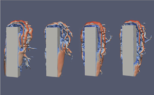
In the present unforced case, switching between antisymmetric and symmetric vortex shedding is not triggered by any external forcing but occurs randomly during the simulations. To understand further this switching phenomenon, the flow field during a switch was investigated in more detail. Figure 8 shows 3-D snapshots of the pressure iso-contours at different time points, exhibiting the switching process from antisymmetric vortex shedding to symmetric. These time points correspond to the switching process highlighted by the circles in figure 9. The downwash flow near the free end caused by flow separation interacts strongly with the spanwise vortex structures near the top, and Wang & Zhou (Reference Wang and Zhou2009) suggested that the free-end downwash flow could suppress the antisymmetric vortex shedding and promote the formation of symmetric vortices. Under the influence of the downwash flow, the switching from antisymmetric to symmetric vortex shedding occurs near the top of the building first. Figure 8 exhibits the flow structure at the initial stage of this switching. At  $t_1$, shed vortices can be observed on both two sides of the building near the top, showing the feature of symmetric vortex shedding, while the flow lower down the building remains antisymmetric. As time progresses, the symmetric vortex shedding gradually extends down the building, with only the near ground flow remaining antisymmetric at $t_4$. Therefore, we observe that the switching from antisymmetric to symmetric vortex shedding does not occur in the entire coherent wake structure simultaneously, but appears first at the top of the building, and then gradually transmits towards the near ground.
Instantaneous snapshots of iso-contours of pressure taken at  $C_p=-0.2$, coloured by velocity. Flow is in the $+x$-direction.

Variation of instantaneous pressure coefficient on side faces at (a)  $z=0.9H$, (b) $z=0.5H$, (c) $z=0.2H$, where $C_{pl}$ and $C_{pr}$ are the pressure coefficient averaged over a line on the left and right side faces at every height. Black circles indicate the symmetric vortex shedding.

Figure 9 shows the time history of the pressure coefficient on the left and right side faces of the building at different heights, where the transient stage has been removed. The symmetric vortex shedding is seen to emerge near the top of the building first and then extend towards the near ground, lasting longer near the top of the building. Moreover, figure 9 reveals that the appearance of the symmetric vortex shedding process is more like an interruption, with the antisymmetric vortex shedding dominating most of the time. Interestingly, immediately prior to and after intervals of symmetric vortex shedding, the antisymmetric vortex shedding ends and restarts with the same orientation. Streamlines for the initial symmetric and symmetric-back-to-antisymmetric shedding are shown in figure 10, corresponding to times  $t = 1.5$ and 1.6 s in figure 9(b). In both images of figure 10, the larger antisymmetric vortex immediately behind the building is closer to side A. Of the small counter-rotating vortices on sides A and B, the strength of the one on side A appears suppressed by the large shed vortex behind the building, and is the slightly weaker of the two.
Instantaneous streamlines and streamwise velocity field in horizontal slices at  $z=0.5H$:(a) initiation of symmetric vortex shedding at $t=1.5$ s; (b) transition from symmetric back to antisymmetric vortex shedding at $t=1.6$ s. Red circles indicate the counter-rotating vortices.

To further investigate the coherent structures present, modal decomposition was applied to snapshots of the 3-D pressure field for the near wake behind the building. To account for the observation that the symmetric vortex shedding behaviour occurs intermittently in short bursts, exhibiting no obvious periodicity (Bisset, Antonia & Browne Reference Bisset, Antonia and Browne1990; Zhou & Antonia Reference Zhou and Antonia1993; Porteous, Moreau & Doolan Reference Porteous, Moreau and Doolan2017; Wang et al. Reference Wang, Zhao, He and Zhou2017), proper orthogonal decomposition (POD) was chosen to obtain the most energetic wake modes in preference to methods that yield structures at a given frequency, such as dynamic mode decomposition (DMD) or spectral POD (Taira et al. Reference Taira, Brunton, Dawson, Rowley, Colonius, McKeon, Schmidt, Gordeyev, Theofilis and Ukeiley2017). Snapshots of the pressure field with its mean component subtracted from the sampled data were analysed. The results are summarised in figure 11, showing the energy content of first six pressure POD modes. The first two modes, which account for nearly 40  $\%$ of the overall energy, are shown in figure 11(a). They exhibit coherent vortex structures that are antisymmetric about the wake centreline over the entire building height, confirming that the large-scale von Kármán antisymmetric vortex shedding mode is prevalent in the near wake. The spectra of the first two modes are shown in figure 12, exhibiting peaks at the antisymmetric vortex shedding frequency, $St_B= 0.1$. For a horizontal slice at $z=0.5H$, the first two modes of the pressure field are shown in figure 11(b). The antisymmetric spanwise vortex shedding with separation near both leading edges is again observed.
First two POD modes of the pressure fluctuation: (a) 3-D POD modes and their corresponding spatial structures are plotted using the iso-contour of dominant amplitude; (b) POD modes plotted on the horizontal slice at  $z=0.5H$.

Normalized spectra of the first two 3-D POD modes.

In order to design a controller that attenuates the unsteady loading via attenuation of wake unsteadiness, it is necessary to know the frequency content of the unsteady fluctuations. The normalised power spectral density (PSD) of the side-force (lift) coefficient  $C_l$ at different heights of the building is shown in figure 13. The main spectrum peak in $C_l$ occurs at the same frequency $St_B=0.1$ along the entire building height, in good agreement with the dominant frequency reported in the experimental study of Obasaju (Reference Obasaju1992). Interestingly, it can be found that the peak frequency determined by the spectrum of $C_l$ is consistent with the antisymmetric vortex shedding one. This illustrates that even though the average velocity and turbulence intensity of the oncoming flow vary with height, the flow forms an overall vortex structure, with a consistent dominant vortex shedding frequency, as indicated by the 3-D POD modes.
Power spectral density of  $C_l$ at different heights of the CAARC building, where $C_l$ stands for the coefficient of the $y$-direction integrated pressure force at every height, and $St_B=fB/U$ is the Strouhal number based on the building width $B$. Filtering is applied using the pwelch function for clarity.

3.3. Effects of the atmospheric boundary layer
As many studies have considered an FWMC in the presence of a uniform inflow, it is insightful to consider explicitly the effect of the atmospheric boundary layer on the flow features. This is now achieved by performing a simulation with a uniform oncoming flow incident on the CAARC building. The same baseline mesh as for the atmospheric boundary layer case was used, and a steady uniform velocity profile corresponding to  ${{Re}_B}=24\ 000$ was set as the inlet boundary condition. The boundary layer was set to zero height at the inlet, and a very thin boundary layer developed between the inlet and the building, with thickness less than 10 % of the building height.
The r.m.s. value for  $C_l$ in the uniform inflow was found to be 0.038, significantly lower than the value 0.29 for the atmospheric boundary layer flow. The spectra of $C_l$ are compared for the atmospheric boundary condition and uniform inflow in figure 14(a); the peak frequencies are very close, both corresponding to antisymmetric vortex shedding. The PSD spectra of $C_d$ are compared in figure 14(b). It is observed that for the atmospheric boundary layer flow, the peak occurs at the low frequency $St_B\sim 0.02$, in good agreement with the experimental data from Obasaju (Reference Obasaju1992). However, this spectral peak is not seen in the uniform inflow case, which is consistent with the suggestion by Obasaju (Reference Obasaju1992) and Kwok (Reference Kwok1982) that this peak is associated with the inflow turbulence rather than the wake.
(a) Normalised spectra of the building's side-force fluctuation  $C_l$. (b) PSD of $C_d$ of the building with two inflow conditions. Filtering is applied using the pwelch function for clarity.

Figure 15 shows the pressure fluctuations on side faces of the building in the atmospheric boundary layer case and the uniform inflow case. Here,  $C_{pl}'$ and $C_{pr}'$ denote the fluctuations of the pressure coefficient on the left and right side faces, respectively; the scatter plots show the instantaneous results of 40 000 samples. These scatter plots reflect the symmetry of fluctuations for horizontal slices at different heights.
Scatter plots for the fluctuation of the pressure coefficient on the building side faces, with(a) atmospheric boundary layer inflow, and (b) uniform inflow at different heights.

For the uniform inflow at  $z=0.9H$, i.e. near the top, most scatter points are located in the first and third quadrants, with the correlation coefficient $R$ between $C_{pl}'$ and $C_{pr}'$ being $0.8215$. Thus the pressure fluctuations on opposing side faces are in phase most of the time, indicating that symmetric vortex shedding dominates. However, for the building immersed in the atmospheric boundary layer, the scatter plot slants the other way, with the pressure fluctuations on two opposing faces being negatively correlated at $z=0.9H$, with correlation coefficient $-0.3219$. Similarly at $z=0.5H$, the correlation coefficients between $C_{pl}'$ and $C_{pr}'$ are $-0.4863$ for the atmospheric boundary layer inflow and $-0.0612$ for the uniform inflow, while at $z=0.2H$ they are $-0.6632$ and $-0.0916$, respectively. All of this indicates that the presence of the atmospheric boundary layer enhances the antisymmetric vortex shedding behaviour and inhibits the symmetric vortex shedding behaviour compared to the uniform inflow. The tendency to the antisymmetric behaviour is stronger close to the ground for both flows.
4. Feedback control
We now seek to develop and test active feedback control techniques to attenuate the unsteady loading of the CAARC high-rise building in an atmospheric boundary layer flow. The chosen actuator and sensor signals are presented first, after which two feedback control strategies are described. This is followed by the presentation of the system identification and the implementation of the feedback controllers in numerical simulations.
4.1. Choice of sensor signals
As the aim of feedback control is to attenuate the unsteady loading on the building, we seek a sensor signal that is capable of capturing this unsteady loading. Furthermore, the sensor should be located on the building surfaces, for future practical applicability, and ideally should require measurements on as few of the building surfaces as possible.
Kwok (Reference Kwok1982), Liang et al. (Reference Liang, Liu, Li, Zhang and Gu2002) and Gu & Quan (Reference Gu and Quan2004) indicated that the wind-induced structural response of super-tall buildings in the cross-wind direction is usually much larger than the along-wind one. Hence the present study will focus on attenuating the cross-wind loading (i.e. the fluctuating lift coefficient). While the unsteady lift coefficient can be measured directly using pressure sensors on the two side surfaces of the building, it may also be possible to exploit the dominance of the antisymmetric vortex shedding mode in the wake to sense only on the building base (rear face). A possible choice of sensor signal is that of the vertically antisymmetric component of the base pressure force, which can be obtained by taking the integrated value of the pressure on the base and counting as negative the values on one horizontal half, as shown schematically in figure 16(a). This choice would be consistent with that for other bluff-body flows dominated by antisymmetric vortex shedding (Flinois & Morgans Reference Flinois and Morgans2016; Dalla Longa et al. Reference Dalla Longa, Morgans and Dahan2017), and involves pressure measurement on just one of the five exposed building surfaces.
(a) Schematic of the antisymmetric base pressure force signal. (b) Normalised FFT spectra of the building's side-force fluctuation  $C_l$ and the antisymmetric base pressure force signal, all in the absence of any actuation.

Figure 16(b) compares the spectra of the building's variations in  $C_l$ and the antisymmetric base pressure force. Both the sensor signal and $C_l$ exhibit a narrow peak at $St_B= 0.1$, confirming that the proposed sensor signal captures the main vortex shedding features of the unsteady loading. As a further check, the cross PSD between $C_l$ and the antisymmetric pressure force was found to exhibit a magnitude peak value of 0.8 at $St_B= 0.1$, confirming significant coherence between $C_l$ and antisymmetric base pressure force. Thus the antisymmetric base pressure was chosen as the sensor signal for feedback control.
4.2. Choice of actuator
We seek an actuator strategy that has the spatial location, spatial form and control authority to attenuate the unsteady loading. The strategy should also be implementable in real experiments outside of the wind or water tunnel, even though the present study uses computational flow simulations as a test-bed.
The unforced flow shown in figure 11(b) reveals that the antisymmetric vortex shedding that is the main cause of unsteadiness involves large-scale flow separation from the leading edges of the building. This suggests that actuation along these leading edges will have good control authority. By choosing the signals on either edge to be out of phase with one another, the antisymmetric nature of the vortex shedding can be accounted for.
We therefore choose actuation in the form of synthetic slot jets, implemented near the leading edges of the building. The synthetic jets extend along the entire cylinder span (height) with slot width  $0.04B$ and injection angle 45 $^{\circ }$, as shown in figure 17(a). The two synthetic slot jets located on different lateral edges are out of phase and operate simultaneously.
(a) Set-up of the body-mounted sensing and actuation. (b) Frequency domain model underpinning the linear feedback control strategy, with  $s$ denoting the Laplace transform variable.

4.3. Linear control strategy
A linear SISO feedback controller is now designed, whose aim is to attenuate the sensor signal fluctuations and thus attenuate the unsteady loading on the building.
The feedback control approach is summarised in the schematic in figure 17(b). Fluctuations in the antisymmetric base pressure sensor signal  $Y(s)$ occur due to both natural disturbances in the unforced flow, $N(s)$, and the response to actuation, $U(s)$, where $s={\rm i}\omega$ is the Laplace transform variable. The transfer functions $H(s)$ and $G(s)$ are those describing how the sensor signals respond to the natural disturbances and actuation, respectively – initially, they are unknown, but they can be identified if needed. It then follows that the sensor signal in the presence and absence of control can be written as
 $$\begin{gather} Y{(s)_{{without\ control}}} = U(s)\,G(s) + N(s)\,H(s), \end{gather}$$
 $$\begin{gather}Y{(s)_{{with\ control}}} = \frac{{U(s)\,G(s) + N(s)\,H(s)}}{{1 + G(s)\,K(s)}}. \end{gather}$$
The ratio of sensor signal fluctuations with and without control is then given by
 \begin{equation} \left| {\frac{{Y{{(s)}_{{with\ control}}}}}{{Y{{(s)}_{{without\ control}}}}}} \right| = \frac{1}{{| {1 + G(s)\,K(s)} |}} = | {S(s)} |, \end{equation}
where  $S(s)$ is what is known as the sensitivity transfer function (Golnaraghi & Kuo Reference Golnaraghi and Kuo2017). Thus, by designing the frequency response of $|S({\rm i}\omega )|$ to be less than unity at the frequencies most relevant to the sensor fluctuations, attenuation of the sensor signal fluctuations at these frequencies will be achieved. The steps involved in this process are (i) identifying the frequency response for the transfer function $G(s)$, and (ii) designing a feedback controller $K(s)$ such that $| {S({\rm i}\omega )} | < 1$ over the most important frequencies, which are those for which the spectra in figure 16(b) exhibit high values.
This approach to feedback control for sensor signal attenuation has been implemented successfully in other flow control applications (Dahan et al. Reference Dahan, Morgans and Lardeau2012; Dalla Longa et al. Reference Dalla Longa, Morgans and Dahan2017; Evstafyeva et al. Reference Evstafyeva, Morgans and Dalla Longa2017). It should be noted that some fundamental limits on the shape of  $|S({\rm i}\omega )|$ exist, including that $|S({\rm i}\omega )|<1$ cannot be achieved over all frequencies. A ‘waterbed’ effect exists by which it being less than unity over some frequency range implies that it will exceed unity over other frequency ranges (Golnaraghi & Kuo Reference Golnaraghi and Kuo2017).
4.4. LMS control strategy
The LMS controller is an adaptive controller whose parameters are optimised by the LMS algorithm. This algorithm aims to minimise the mean square of the error signal. It has been effective in both combustion instability control (Billoud et al. Reference Billoud, Galland, Huynh and Candel1992; Evesque & Dowling Reference Evesque and Dowling2001) and transition delay control (Kurz et al. Reference Kurz, Goldin, King, Tropea and Grundmann2013; Fabbiane et al. Reference Fabbiane, Bagheri and Henningson2017). As the aim is to attenuate the high-rise building's side-force fluctuations, the sensor signal  $y$, given by antisymmetric base pressure fluctuations, is chosen as the error signal in this LMS algorithm.
The configuration of the LMS feedback control is shown in figure 18. The actuation signal to be generated by the LMS controller is prescribed by an infinite-impulse-response (IIR) filter (Widrow et al. Reference Widrow, McCool, Larimore and Johnson1977)
 \begin{equation} u(t) = \sum_{i = 0}^{n - 1} {{a_i}(t)\,y(t - i\, {{\rm d}}T) + \sum_{j = 1}^{m} {{b_j}} } (t)\,u(t - j\, {{\rm d}}T), \end{equation}
where  $u(t)$ and $y(t)$ are the time-discrete actuation and sensor signals, respectively, and ${{\rm d}}T$ is the control sampling interval time. The computations for the coefficients $a_i$ and $b_j$ are the kernels of this adaptive controller. The LMS algorithm is employed to update dynamically these controller coefficients at each time step in order to minimise the mean square of the sensor signal $y$, as follows:
 \begin{equation} \left.\begin{array}{c@{}}
{a_i}(t + {{\rm d}}T) = {a_i}(t) - \mu\,y(t)\,{\delta _i}(t),\\ {b_j}(t + {{\rm d}}T)
= {b_j}(t) - \mu\,y(t)\,{\gamma
_j}(t), \end{array}\right\} \end{equation}
\begin{equation} \left.\begin{array}{c@{}}
{a_i}(t + {{\rm d}}T) = {a_i}(t) - \mu\,y(t)\,{\delta _i}(t),\\ {b_j}(t + {{\rm d}}T)
= {b_j}(t) - \mu\,y(t)\,{\gamma
_j}(t), \end{array}\right\} \end{equation}
where  $\mu$ is the convergence step length and
 \begin{equation} \left.\begin{array}{c@{}}
\displaystyle {\delta _i}(t) = Dy(t - j\, {{\rm d}}T) +
\sum_{k = 1}^{m} {{b_k}(t)\,{\delta _i}(t
- k\, {{\rm d}}T)}, \\ \displaystyle {\gamma
_j}(t) = Du(t - j\, {{\rm d}}T) + \sum_{k = 1}^{m}
{{b_k}(t)\,{\gamma _j}(t - k\, {{\rm
d}}T)}, \end{array}\right\} \end{equation}
\begin{equation} \left.\begin{array}{c@{}}
\displaystyle {\delta _i}(t) = Dy(t - j\, {{\rm d}}T) +
\sum_{k = 1}^{m} {{b_k}(t)\,{\delta _i}(t
- k\, {{\rm d}}T)}, \\ \displaystyle {\gamma
_j}(t) = Du(t - j\, {{\rm d}}T) + \sum_{k = 1}^{m}
{{b_k}(t)\,{\gamma _j}(t - k\, {{\rm
d}}T)}, \end{array}\right\} \end{equation}
where  $D$, named the auxiliary path in the LMS algorithm (Evesque & Dowling Reference Evesque and Dowling2001; Fabbiane et al. Reference Fabbiane, Bagheri and Henningson2017), is the transfer function describing the effect of actuation on the sensor signal. Note that this method is not completely model-free as $D$ needs to be determined. In the current work, the open-loop transfer function $G(s)$ obtained in the linear controller design is adopted as the auxiliary path $D$.The feedback coefficient $b_j$ might be updated adaptively to some values that drive the IIR filter towards instability and cause divergence of the LMS algorithm. An efficient method, proposed by Evesque & Dowling (Reference Evesque and Dowling2001), that checks the stability of the IIR filter and resets the coefficients if unstable, is implemented to ensure the convergence of the LMS controller.
Schematic for the LMS feedback control strategy.

4.5. System identification
It is clear from the above descriptions that a low-order linear model for  $G(s)$ must be identified in order to design both feedback controllers. Note that $H(s)$ in figure 17(b) does not need to be identified.
If we assume (we can later check) that the sensor response induced by open-loop forcing is approximately dynamically linear, then  $G(s)$ can be identified through linear system identification. Different actuation forcing signals can be applied in order to perform system identification, but the most intuitive, that of purely harmonic open-loop forcing, ${U(t)}={A_j^{*}}{U_H}\sin (2{\rm \pi} {f_j}t)$, over a relevant range of frequencies, $f_j$, allows us to obtain high-quality frequency response data while also facilitating a check on the assumption of dynamic linearity, through the ability to vary the amplitude. Based on the spectra of figure 16(b), the open-loop forcing frequency range was chosen to be $0.05 \le St_B\le 1$, with amplitudes ranging from 0.15 to 0.25 considered.
For the harmonic forcing simulations, the harmonic actuator signal was applied and the sensor signal measured. Once transients in the sensor signal had decayed to low levels, the sensor signal was recorded and the gain and phase shift of the open-loop response extracted using spectral analysis. The results, shown in figure 19(a), first confirm that the frequency response varies little with forcing amplitude  $A_j$ for all frequencies across the considered range. Hence the response of the sensor signal to the forcing can be considered dynamically linear. The average gains and phase shifts across the different forcing amplitudes are calculated, and the Matlab fitfrd command used to fit the frequency-domain response data with a fifth-order state-space model, as shown in figure 19(a).
Frequency response – gain and phase shift for: (a) system identification data resulting from open-loop harmonic forcing as well as a fifth-order fit from the Matlab fitfrd command; (b) the designed controller  $K(s)$ and sensitivity function $S(s)$.

4.6. Controller design and implementation
4.6.1. Linear controller design
To suppress the fluctuations in the sensor signal, the feedback controller  $K(s)$ is designed such that the magnitude of the sensitivity transfer function in (4.3) is less than unity over the frequency range where the wake exhibits significant dynamics. Based on the unforced spectra in figure 16(b), the main frequency to target for attenuation is $St_B = 0.1$.
Conventional loop-shaping is used to design the feedback controller  $K(s)$ to achieve this. The final feedback controller is a combination of a first-order high-pass filter and a second-order band-pass filter, written as
 \begin{equation} K(s) = \frac{{167.7{s^{2}} }}{{{s^{3}} + 100.5{s^{2}} + 1684s + 23\ 520}}. \end{equation}
The gain and phase shift of the controller  $K(s)$, along with the resulting sensitivity $S(s)$, are shown in figure 19(b), where it can be seen that $S(s)<1$ is achieved at and around $St_B = 0.1$.
4.6.2. LMS controller design
In terms of the LMS controller, a second-order IIR filter is used to generate the controller signal, i.e.  $m=n=2$. The convergence step length $\mu$ has been chosen as a constant, with its value less than the upper bound $1/(m + 1)\sigma _y^{2}$, to avoid LMS algorithm divergence (Madisetti Reference Madisetti1997). The open-loop transfer function $G(s)$, obtained through linear system identification, is adopted as the auxiliary path $D$. In the initial stage of adaptive updating of controller coefficients, the LMS controller may produce large actuation amplitudes that could induce the divergence of the numerical iterations, thus a saturation limit of the actuation signal is applied.
4.6.3. Effect of feedback controllers
The controller was implemented in discrete-time format in the LES simulations in order to test its performance. When implementing the feedback flow control into the flow simulations, the actuators, whose signal at each time step is generated following the variation of the sensor signal, require a time-varying boundary condition. Here, the plugin SWAK4FOAM (SWiss Army Knife for OpenFOAM) library allowing user-defined equations for boundaries was used.
The effects of the linear and LMS controllers on the sensor signal and the lift coefficient are shown in figure 20. Both controllers are effective in attenuating successfully the sensor signal fluctuations over the targeted frequency range, although high frequencies are amplified with the LMS controller. The r.m.s. fluctuations in  $C_l$ were reduced correspondingly by approximately 38 $\%$ and 17 $\%$ via the linear and LMS controllers, respectively, as shown in figures 20(b) and 20(d). In order to understand the mechanism of our controller, a POD analysis of the unforced and controlled flows based on the fluctuating kinetic energy was conducted to illustrate the difference in their unsteady flow structures. Figure 21 shows the streamwise velocity components of the first POD mode at $z=0.5H$ for the feedback controlled flows compared to the unforced flow. It is observed that the centre of the coherent structures, which is located at around $x/B=1.2$ in the unforced flow, moves towards around $x/B=1.6$ under the effect of the linear feedback controller.The linear feedback controller pushes the dominant coherent structures corresponding to antisymmetric vortex shedding further downstream, while the LMS controller affects the antisymmetric vortex shedding only mildly. Overall, the linear feedback controller outperforms the LMS one with regard to the attenuation of the side-force fluctuation. The changes to the time-averaged flow field after implementing feedback control are shown in figure 22. The recirculation region has been extended in the streamwise direction, in a manner similar to that for the D-body flow investigated by Dalla Longa et al. (Reference Dalla Longa, Morgans and Dahan2017). In summary, the controller delays the formation of dominant vortices, which can reduce further the pressure fluctuations on the building caused by these vortices.
Effect of control: (a) spectra for antisymmetric base pressure force signal with linear feedback control; (b) time variation of building side-force (lift) coefficient with linear feedback control;(c) corresponding actuation signal with linear feedback control; (d) spectra for antisymmetric base pressure force signal with LMS feedback control; (e) time variation of building side-force (lift) coefficient with LMS feedback control; ( f) corresponding actuation signal with LMS feedback control.

Streamwise velocity components of the first POD mode at  $z=0.5H$ for: (a) unforced flow;(b) flow with the linear controller; (c) flow with the LMS controller.

Colour contours of the time-averaged streamwise velocity and line contours of the stream function: (a) unforced flow; (b) linear controlled flow.

The aim of the LMS algorithm is to minimise the mean square of the error signal. In this work, the performance of the LMS controller is effective but not as good as for the linear controller. This may be attributed to the way in which the auxiliary path is prescribed. As described in § 4.4, our approach employed an offline system identification based on the assumption of dynamic linearity. It may be the case that this approach does not account sufficiently for nonlinearity or changes in the auxiliary path as control is implemented.A more accurate online estimate of this auxiliary path may improve the performance of the LMS controller.
5. Feedback control with reduced sensing area
The above feedback control strategy uses a sensor signal that depends upon the pressure integrated over the entire rear face (base) of the building, as shown in figure 16(b). In order to reduce the complexity of sensing and the total number of individual sensors required, a controller is now investigated that is based upon sensing over a smaller building rear-face area.
As the dynamic response of a high-rise building to unsteady loading can be approximated by that of a cantilever beam pinned at its lower end to the ground, the effect of unsteady loading towards the top of the building will have more effect on motion amplitude and hence occupant comfort. At the same time, the antisymmetric vortex shedding mode that dominates the unsteady loading is predominant towards the middle of the building, as shown in figure 11, with downwash and upwash flows becoming more influential towards the top and bottom, respectively. For these reasons, a sensing area that extends over the upper part of the building base, but not as far as the top, i.e. from 0.4 $H$ to 0.8 $H$, is investigated, as shown in figure 23(a). The sensing again takes the asymmetric component of this pressure force over this reduced area. The unforced spectrum of this new sensor signal is shown in figure 23(b), exhibiting a frequency peak similar to that of full base sensing in figure 16(b).
(a) Set-up of the body-mounted sensors and actuation for the new feedback strategy. (b) Spectrum of the partial antisymmetric pressure signal for unforced flow.

Having a better performance than the LMS controller, the linear feedback control strategy described in § 4.3 is chosen to check the feasibility of this reduced sensing area, and the actuation is implemented as shown in figure 17. The modified open-loop frequency response, identified through harmonic forcing simulations, is shown in figure 24(a). It exhibits little dependence on the input forcing amplitude, implying dynamic linearity. The fifth-order linear state-space model  $G_n(s)$, resulting from a fit through these points using Matlab's fitfrd function, is also shown in figure 24(a), exhibiting a form similar to that with full base area sensing. The feedback controller $K_n(s)$ was designed by loop-shaping in the frequency domain to give low sensitivity close to frequencies $St_B = 0.1$; its phase and gain along with the resulting sensitivity function are shown in figure 24(b), where it can be seen that $|S(s)|<$1 is achieved close to $St_B = 0.1$.
Frequency response – gains and phase shifts for: (a) system identification data for open-loop forcing with fewer sensors; (b) designed controller  $K_n(s)$ and sensitivity function $S_n(s)$.

This feedback controller, based upon a reduced sensing area, was implemented in simulations. The sensor (partial antisymmetric base pressure force) signals are compared in both the absence and presence of feedback control in figure 25, along with the building's side-force (lift) coefficients. Control is seen to achieve its primary objective of attenuating the sensor signal fluctuations, giving corresponding attenuation in the fluctuations of  $C_l$ of approximately 35 $\%$, demonstrating that feedback control with reduced sensing area is feasible.
Effect of the controller with fewer sensors – comparison between cases with and without feedback control in: (a) spectrum for antisymmetric base pressure signal; (b) time history for lift coefficient.

6. Conclusion
In this work, the flow structures around a high-rise building immersed in an atmospheric boundary layer were studied numerically using wall-resolved large eddy simulations.A canonical high-rise building, known as the CAARC model, was studied, which has a constant rectangular cross-section. An oncoming wind normal to the wider dimension was considered.
The flow features were found to be three-dimensional, with two types of spanwise vortex shedding evident, along with a downwash flow over the building top, and an upwash flow near the building/ground interface. The flow changes intermittently between antisymmetric vortex shedding, which exhibits a dominant frequency, and symmetric vortex shedding, which is not associated with a dominant frequency. The switching from antisymmetric to symmetric vortex shedding mode transmits gradually from the top of the building towards the near ground, and the region near the top maintains the symmetric vortex shedding longer. Proper orthogonal decomposition confirmed that the large scale von Kármán antisymmetric vortex shedding mode is prevalent in the near wake, rather than the symmetric mode. This mode dominates the unsteady loading on the building. The influence of the atmospheric boundary layer was also analysed via the comparison with the uniform inflow case, with it being found that the symmetric vortex shedding mode gets suppressed significantly when the building is fully immersed in the atmospheric boundary layer.
Two feedback control strategies were then developed, which aimed to attenuate the building's unsteady loading. The control strategies were implemented via body-mounted sensors and actuation, for practical applicability. Sensing was chosen to be the vertically antisymmetric component of the base pressure force on the building's rear face, allowing the most important features of the unsteady loading to be captured through measurements on only one building face. Actuation was via zero-net mass flux (unsteady slot jet) actuation along the two leading edges of the building, constant along each edge, and with actuation along each edge in antiphase with the other.
System identification of the sensor signal unsteady response to actuation was performed, using harmonic forcing of the actuator signal across relevant frequencies and amplitudes. A linear feedback controller base on the frequency-domain loop-shaping method and an LMS adaptive controller were then designed to attenuate the sensor unsteadiness in the presence of feedback control. The designed controllers were implemented in large eddy simulations, and attenuated successfully the building's side-force fluctuations by 38  $\%$ and 17 $\%$, respectively. A further study showed that reducing the sensing to 40 $\%$ of the building's rear face area led to similar successful linear feedback control. This work can provide a theoretical basis for the practical application of this novel active control approach to high-rise buildings. We envisage this being a starting point for further investigating a feedback control for mitigating the unsteady flow on high-rise buildings, with differing oncoming wind angles being further explored in our future studies.
Acknowledgements
Both the Imperial College High Performance Computing facilities and ARCHER (the UK National Supercomputing service) used in this work are acknowledged.
Funding
This research was supported by the Imperial College President PhD Scholarship scheme.
Declaration of interests
The authors report no conflict of interest.


 Open access