





1. Introduction
Resonant periodic waves, either at the free surface or internal, can be observed in rectangular and cylindrical cavities (Stoker Reference Stoker1992), as well as in basins with a more complicated shape (Rycroft & Wilkening Reference Rycroft and Wilkening2013; Geva et al. Reference Geva, Bukai, Zemach, Gabay, Krakovich and Shemer2021). In the framework of linear theory, the governing equations and boundary conditions define the dispersion relation between the wavevectors and frequencies. In a closed cavity partially filled with liquid, a discrete wave vector spectrum of standing gravity waves excited by either random or regular forcing is defined by the geometry. If dissipation is weak, only those permitted standing waves can exist in the cavity; when not sustained by sufficient forcing, they decay due to the friction at the cavity's walls (Keulegan Reference Keulegan1959; Hill Reference Hill2003). The external energy input enables sustainable standing waves; it also introduces to the system frequencies present in the forcing spectrum. If the forcing spectrum contains frequencies sufficiently close to those corresponding to one of the possible spatial wave modes, the linear model predicts the excitation of a forced steep standing wave in the cavity. In this case, the contribution of dissipation and nonlinearity needs to be considered (Moiseev Reference Moiseev1958).
Resonant surface standing gravity waves in rectangular cavities generated in experiments by lateral harmonic oscillations were studied by Faltinsen (Reference Faltinsen1974), Lepelletier & Raichlen (Reference Lepelletier and Raichlen1988) and Faltinsen et al. (Reference Faltinsen, Rognebakke, Lukovsky and Timokha2000); excitation by rolling motion was applied in Grotle, Bihs & Æsøy (Reference Grotle, Bihs and Æsøy2017). The wave amplitudes in those experiments were determined by measuring the instantaneous surface elevation at several locations within the cavity. The associated theoretical models that account for cubic nonlinearities lead to the Duffing equation for the amplitude of the resonant mode (Faltinsen Reference Faltinsen1974; Hill Reference Hill2003). The resulting response curve pattern varies qualitatively depending on the ratio between the resonant wavelength and the mean liquid depth. For surface gravity waves in a cavity with depth  $\tilde {H}$, the radian frequency $\tilde{\omega}$ is related to the wave vector $\tilde {\boldsymbol {k}} =(\tilde {k}_x,\tilde {k}_y)$, $x$ and $y$ being horizontal orthogonal coordinates, by the dispersion relation $\tilde {\omega }^2=g|\tilde {\boldsymbol{k}}| \tanh (|\tilde {k}|\tilde {H})$, where $g$ is the acceleration due to gravity, $|\tilde {\boldsymbol{k}}|^2=(\tilde {k}_x^2+\tilde {k}_y^2)$, tildes denote dimensional values. For the deep-water case ( $|\tilde {\boldsymbol{k}}|\tilde {H}\gg 1$), the response curve corresponds to the softening spring, and the effective resonance frequency decreases with an increase in the forcing amplitude. In shallow water $|\tilde {\boldsymbol{k}}|\tilde {H}\ll 1$, an opposite effect is observed (Ockendon & Ockendon Reference Ockendon and Ockendon1973). Numerical simulations of waves excited by cavity motion (Frandsen Reference Frandsen2004; Liu & Lin Reference Liu and Lin2008) support those conclusions for an arbitrary harmonic excitation. Excitation of standing waves by a pair of piston-type wavemakers at opposite walls of a rectangular cavity is equivalent to lateral shaking, as long as the friction at the walls can be neglected (Agnon & Bingham Reference Agnon and Bingham1999; Paprota Reference Paprota2023). A pair of pistons has also been used to generate standing internal waves (Thorpe Reference Thorpe1968).
Wave tanks can be seen as cavities with sidewalls at  $\tilde {x}=0$ and $\tilde {x}=\tilde {L}$, wavemaker at $\tilde {y}=0$ and waves allowed to propagate to $\tilde {y}\to \infty$. For sufficiently deep water, standing waves with wavevector components $\tilde {k}_{x,n}=n{\rm \pi} /\tilde {L}$, $n$ being the mode number, can be excited in such facilities by a specially configurated wavemaker located at one end of the tank (Barnard, Mahony & Pritchard Reference Barnard, Mahony and Pritchard1977; Kit, Shemer & Miloh Reference Kit, Shemer and Miloh1987), provided the forcing is periodic at frequency $\tilde {\omega }$ sufficiently close to one of the natural tank frequencies $\tilde {\omega }_n=\tilde {\omega }(\tilde {k}_{x,n},0)$. For small detuning $|\tilde {\omega }/\tilde {\omega }_n-1|\ll 1$, the dispersion relation requires a non-zero wavevector component along the tank $|\tilde {k}_y |\ll \tilde {k}_{x,n}$. In the framework of the linear theory (Wehausen Reference Wehausen1974; Shemer, Kit & Miloh Reference Shemer, Kit and Miloh1986; Fu et al. Reference Fu, Zhou, Li, Shemer and Arie2017), for forcing at frequency $\tilde {\omega }<\tilde {\omega }_n$, $\tilde {k}_y$ is imaginary and the standing wave envelope decays with distance as $\exp (-|\tilde {k}_y|\tilde {y})$. At forcing frequencies $\tilde {\omega }$ exceeding $\tilde {\omega }_n$, the wavenumber component $\tilde {k}_y$ is real; the standing wave envelope propagates as a slow running wave along the test section. Close to the resonance, where linear inviscid theory predicts large amplitudes and thus breaks down, nonlinear effects need to be considered (Kit et al. Reference Kit, Shemer and Miloh1987). The temporal and spatial evolution of the resonant standing waves in the vicinity of resonance is adequately described by the cubic Schrödinger equation (CSE). It was demonstrated by Shemer & Kit (Reference Shemer and Kit1988) that manipulating dissipation at solid surfaces by adding roughness element faces can strongly affect the observed standing wave pattern. The results of the CSE model that accounts for dissipation at sidewalls and at the wavemaker yield both qualitative and quantitative agreement with experiments carried out in the vicinity of the linear resonant frequency. Computations carried out on the basis of this theoretical model accurately predict the diverse patterns observed for such directly excited resonant standing waves as a function of the forcing amplitude and frequency, such as appearance and propagation along the tank of envelope solitons, Fermi–Pasta–Ulam recurrence at slow time scale, chaotic modulation, hysteresis, etc. (Shemer Reference Shemer1990).
Cross-waves represent another example of the two-dimensional system with qualitatively different behaviour in the  $\tilde {x}$ and $\tilde {y}$ directions. Those resonant standing waves in a long rectangular wave tank can be excited by a plane wavemaker that operates at a sufficiently high amplitude at a frequency close to the double natural frequency corresponding to the tank width, $2\tilde {\omega }_n$ (Jones Reference Jones1984; Lichter & Shemer Reference Lichter and Shemer1986). The resulting cross-waves, in this case excited by subharmonic parametric resonance, may have amplitudes higher than those of propagating waves at the wavemaker forcing frequency. Those nonlinear cross-waves are also described by CSE; the difference between the theoretical models describing standing waves that are generated directly at the wavemaker forcing frequency, and parametrically excited subharmonic cross-waves, is mainly in the boundary condition applied at the wavemaker (Kit & Shemer Reference Kit and Shemer1989; Shemer & Kit Reference Shemer and Kit1989). Wave patterns identified in parametrically excited subharmonic standing wave fields resemble those observed in the case of direct excitation; however, due to the more complicated wave generation mechanism, the CSE-based cross-wave model only yields qualitative agreement with experiments.
All those studies consider standing waves in rectangular basins for which the linear theory allows the existence of standing waves with wave vectors  $\boldsymbol{k} =(\tilde{k}_x,\tilde {k}_y)$ that satisfy the linear dispersion relation, with at least one of the wavevector components being real, while the other one can be either real or imaginary. Contrary to that, we study here standing waves excited in a deep stationary narrow rectangular cavity with length $\tilde {L}$ and width $\tilde {B}\ll \tilde {L}$. The narrow geometry eliminates the possibility of existence of standing waves with cross-cavity wavenumber component $\tilde {k}_y<{\rm \pi} /\tilde {B}$. Therefore, when waves are excited in such a cavity at a frequency $\tilde {\omega }$ close to that of one of the natural longitudinal standing waves $\tilde {\omega }_n=\tilde {\omega }({\rm \pi} n/\tilde {L})$, the linear deep water dispersion relation $\tilde {\omega }^2=g|\tilde {\boldsymbol{k}}|$ is not satisfied for a single longitudinal spatial mode. In view of these considerations, the resonant standing waves under constraints imposed by the geometry need to contain additional wave components at the forcing frequency but with a discrete wavenumber spectrum. The resulting complicated wave field is considered in the present experimental and theoretical study.
The remainder of the paper is organized as follows. Section 2 describes the experimental facility and presents the initial observations. The theoretical model given in § 3 contains linear theory for infinitely small waves and its extension that accounts for weakly nonlinear effects. The theoretical results are validated by comparison with measurements in § 4. The concluding remarks are given in § 5.
2. Experimental facility
Experiments are performed in a rectangular cavity with length  $\tilde {L}=772$ mm and width $\tilde {B}=160$ mm that is made of clear glass and filled with water to a depth of $\tilde {H}\sim 400$ mm (figure 1). The walls of the cavity are high enough to prevent water splashing out. Waves are excited by a cylinder with the radius $\tilde {R}=21$ mm and length a few millimetres shorter than $B$; its axis spans the cavity parallel to the short wall. The wavemaker is placed under the water surface with its centre at depth $\tilde {h}$. A computer-controlled linear motor (Linmot C20) forces it to oscillate harmonically in the vertical direction with the amplitude $\tilde {A}$ and radian frequency $\tilde {\omega }$; the amplitude is limited so the cylinder does not cross the liquid surface. The controller sets the parameters with a precision of 0.01 ms for the period and 0.05 mm for amplitude. The wave excitation by the immersed cylinder has mostly been used so far for the internal waves in stratified liquids (Mowbray & Rarity Reference Mowbray and Rarity1967; Sutherland et al. Reference Sutherland, Dalziel, Hughes and Linden1999). Despite the extensive coverage in the literature of the hydrodynamics of the oscillating immersed bodies (Sumer & Fredsøe Reference Sumer and Fredsøe2006), the theory of surface waves generated by a vertically oscillating cylinder is not yet sufficiently developed.
The scheme of the problem.

The forcing frequency was set in the vicinity of the selected natural frequency
 \begin{equation} \left|\tilde{\omega}^2-g\frac{{\rm \pi} n}{\tilde{L}}\right|\ll g\frac{{\rm \pi} n}{\tilde{L}} = g\tilde{k}_n, \end{equation}
where  $n$ is the natural frequency number. Experiments were performed at $n=2$ and 3 that correspond to the wavelengths $\lambda _2=772$ mm and $\lambda _3=514$ mm ( $\tilde {k}_2=8.14\times 10^{-3}$ mm $^{-1}$, $\tilde {k}_3=12.21\times 10^{-3}$ mm $^{-1}$), long enough to neglect the capillarity effects. For these wavelengths, the wave periods are $T_2=0.7032$ s and $T_3=0.5741$ s, and corresponding radian frequencies are $\tilde {\omega }_2=8.9353$ s $^{-1}$ and $\tilde {\omega }_3=10.943$ s $^{-1}$ satisfying the deep-water dispersion relation. The wavemaker is placed at the distance of $\tilde {L}/n$ from the left wall, corresponding to the wave antinode.
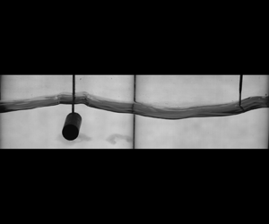
The wavemaker moves at the prescribed frequency and amplitude for more than 700 $T_n$, much longer than the experimentally determined duration of the transient process that does not exceed approximately 150 $T_n$, after which a nearly constant wave amplitude is attained. The wave field is illuminated by LED panels attached to the back wall of the cavity and is recorded at 50 fps by a CCD camera (resolution 2048 by 540 pixels) placed in front of the cavity at a horizontal distance of 2 m from the front wall. The camera's vertical position is 80 cm above the level of the unperturbed water surface. The image is focused on the front wall and the intersection of the free surface with the front wall is clearly seen in the captured images as a black line (figure 2). The vertical lines in the image are the metal rod holding the wavemaker, the joint between two LED panels and the temperature sensor, from left to right. For each frame, the edge detection is performed by analysing a vertical column of pixels corresponding to each lateral position $\tilde {x}$: the location of the point with the maximal vertical pixel intensity derivative defines the instantaneous interface coordinate $\tilde {\zeta }(\tilde {t},\tilde {x})$. A snapshot of a ruler taken by the camera serves for calibration; the pixel size, corresponding to 0.34 mm in the horizontal direction and 0.315 mm in the vertical one, does not change throughout the picture. Experiments were performed for a range of wave periods in the vicinity of $T_2$ and $T_3$ for several wavemaker amplitudes $\tilde {A}$ and depths of the wavemaker $\tilde {h}$. The parameters of the experiments are summarized in table 1, the definitions of the dimensionless parameters are provided in the text below.
A typical example of the captured image (case I). The movie in supplementary material shows two periods in time for case II slowed down by a factor of 5.

Experimental parameters.

The experiments demonstrated resonant-type dependence of the wave amplitude on frequency; the effective resonance frequency corresponding to the maximum wave amplitude depends on the wavemaker amplitude and is always below the natural frequency of the rectangular cavity  $\tilde {\omega }_n$. The wavemaker motion and the surface oscillations above the wavemaker are approximately in phase for frequencies exceeding the effective resonance frequency $\tilde {\omega }_{eff}$. Contrary to that, they are in opposite phases at frequencies below $\tilde {\omega }_{eff}$. Figure 2 indicates that the flow is essentially two-dimensional, justifying the assumption that the waves are characterized by a scalar wavenumber. The boundary conditions at the sidewalls prescribe the discrete spectrum and, unlike the case of the semi-infinite cavity considered by Fu et al. (Reference Fu, Zhou, Li, Shemer and Arie2017), the small width of the cavity prevents spatial modulation. For the forcing frequencies $\tilde {\omega }$ deviating somewhat from $\tilde {\omega }_n$, only a superposition of the multiple spatial modes is needed to satisfy the boundary conditions, resulting in the non-sinusoidal shape of the free surface, as shown in figure 2 and the movie from the supplementary material available at https://doi.org/10.1017/jfm.2024.509. The deviation of the surface from the sinusoidal shape manifests itself at several scales, including steep segments visible in figure 2 and in the movie near the wavemaker. These gravity–capillary ripples with a length of approximately 2 cm decay before reaching the cavity walls and thus do not affect the standing wave pattern (Shemer & Chamesse Reference Shemer and Chamesse1999).
3. Potential flow
The theory describing the phenomena observed in the experiments is now presented. Two-dimensional potential periodic flow at the wavemaker frequency  $\tilde {\omega }$ in infinitely deep water is considered.
The flow is considered in a non-inertial frame of reference where the finite-size wavemaker does not move, but the liquid far away from it has a uniform non-zero velocity corresponding to that of the wavemaker at any given instant. The flow potential is decomposed into a part representing the forcing, and a linear combination of eigenmodes for the cavity with the fixed immersed wavemaker. The forcing potential tends to that of the uniform flow at infinite depth; the eigenmodes vanish there. The free surface boundary conditions provide the equations needed to determine the expansion coefficients into the series of the eigenmodes.
The eigenfrequencies and eigenmodes of the system are considered first, taking into account the finite size of the wavemaker. For infinitely weak forcing, a linear problem is then solved, providing surface shapes and allowing estimates of contributions due to viscous dissipation at different solid surfaces. In the next weakly nonlinear approximation, the finite amplitude of the surface waves is accounted for small relative detuning
 \begin{equation} \left|\frac{\tilde{\omega}^2-\tilde{\omega}_n^2}{\tilde{\omega}_n^2}\right|\ll 1. \end{equation}
3.1. Mathematical formulation
3.1.1. Governing equations
In the absolute frame of reference, the centre of the wavemaker at the mean depth  $\tilde {h}$ below the unperturbed water level moves vertically with the velocity
 \begin{equation} \tilde{U}(\tilde{t})=\tilde{A}\tilde{\omega}\cos \tilde{\omega} \tilde{t}. \end{equation}
The wavemaker frequency  $\tilde {\omega }$ is in the vicinity of the $n$th natural frequency of the cavity $\tilde {\omega }_n=\sqrt {g\tilde {k}_n}$. Horizontally, the wavemaker is at the first antinode of the natural eigenmode, at the distance of $\tilde {L}/n$ from the left wall. In the non-inertial frame of reference connected to the wavemaker, the effective gravity is $g+\tilde {A}\tilde {\omega }^2\sin \tilde {\omega }\tilde {t}$. Cartesian coordinates are used; the origin of the system is located above the wavemaker at the unperturbed water level and the $\tilde {x}$, $\tilde {y}$ and $\tilde {z}$ axes are directed along the long and short cavity walls and upward, respectively. The flow is in $(\tilde {x},\tilde {z})$ plane.
The dimensionless parameters characterizing the forcing frequency  $\alpha$, the wavemaker amplitude $\varepsilon$ and the effective gravitational acceleration $w$ are defined using the dimensional $\tilde {\omega }_n^{-1}$, $\tilde {k}_n^{-1}$ and the wavemaker amplitude $\tilde {A}$ as the scales of time, spatial coordinates and the surface elevation
 \begin{equation} \alpha=\frac{\widetilde{\omega^2}}{g\tilde{k}_n}=\frac{\tilde{\omega}^2}{\tilde{\omega}_n^2},\quad \varepsilon=\tilde{k}_n\tilde{A}, \quad w=\alpha^{{-}1}+\varepsilon\sin t. \end{equation}
The dimensionless coordinates are denoted by the same symbols without tildes, and the horizontal coordinates of the walls are
 \begin{equation} x_L={-}{\rm \pi},\quad x_R=(n-1){\rm \pi}, \end{equation}
while the dimensionless wavemaker immersion depth and radius are
 \begin{equation} h=\tilde{k}_n\tilde{h},\quad R=\tilde{k}_n\tilde{R}. \end{equation}
For  $n=2,\ 3$ in the present experiments (see table 1), $h\sim 10^{-1}$, $R\sim 10^{-1}$, $\varepsilon \sim 10^{-2}$, $|\alpha -1|\sim 10^{-2}$. The dimensionless potential $\varPhi$ related to the dimensional one $\tilde {\varPhi }$ by
 \begin{equation} \tilde{\varPhi}=\tilde{A}\tilde{\omega}\tilde{k}_n^{{-}1}\varPhi, \end{equation}
satisfies the Laplace equation
 \begin{equation} \nabla^2\varPhi=0. \end{equation}
The following boundary conditions are imposed. At infinite depth, the disturbances vanish, and only the frame movement is retained, thus
 \begin{equation} \boldsymbol{\nabla}\varPhi={-}\cos t \boldsymbol{e}_z\quad \text{at } z\to-\infty. \end{equation}
The non-penetration conditions at the cavity walls and the wavemaker lead to vanishing derivatives of the potential in the normal to the solid surface direction
 \begin{gather} \frac{\partial \varPhi}{\partial x}=0\quad x=x_L,\ x_R, \end{gather}
 \begin{gather}\frac{\partial \varPhi}{\partial n}=0\quad \text{at } x^2+(z+h)^2=R^2. \end{gather}
The free surface  $z=\varepsilon \eta$ is defined in the moving frame of reference as
 \begin{equation} \eta=\frac{\tilde{\zeta}}{\tilde{A}}-\sin t, \end{equation}
the kinematic and dynamic boundary conditions are
 \begin{gather} \frac{\partial \varPhi}{\partial t}+\frac{\varepsilon}{2}(\boldsymbol{\nabla} \varPhi)^2 + (\alpha^{{-}1}+\varepsilon \sin t)\eta = 0, \end{gather}
 \begin{gather}\frac{\partial \eta}{\partial t} + \varepsilon\frac{\partial \eta}{\partial x}\frac{\partial \varPhi}{\partial x} = \frac{\partial \varPhi}{\partial z}, \end{gather}
or, equivalently, in the Newman (Reference Newman2018) form
 \begin{align} &\frac{\partial^{2} \varPhi}{\partial t^{2}}+(\alpha^{{-}1}+\varepsilon \sin t)\frac{\partial \varPhi}{\partial z}+2\varepsilon\boldsymbol{\nabla}\varPhi\boldsymbol{\cdot}\boldsymbol{\nabla}\frac{\partial \varPhi}{\partial t} +\frac{\varepsilon^2}{2}\boldsymbol{\nabla}\varPhi\boldsymbol{\cdot}\boldsymbol{\nabla}(\boldsymbol{\nabla}\varPhi\boldsymbol{\cdot}\boldsymbol{\nabla}\varPhi)\nonumber\\ &\quad -\frac{\varepsilon \cos t}{\alpha^{{-}1}+\varepsilon \sin t} \left[ \frac{\partial \varPhi}{\partial t}+\frac{\varepsilon}{2}\boldsymbol{\nabla}\varPhi\boldsymbol{\cdot}\boldsymbol{\nabla}\varPhi\right] =0, \end{align}
 \begin{equation} \eta={-}\frac{1}{\alpha^{{-}1}+\varepsilon \sin t}\left[\frac{\partial \varPhi}{\partial t} +\frac{\varepsilon}{2}\boldsymbol{\nabla}\varPhi\boldsymbol{\cdot}\boldsymbol{\nabla}\varPhi\right]. \end{equation}
The two evolution equations (3.12) are more convenient for simulations of transient waves, while (3.13) is preferable for semi-analytical studies of periodic regimes and used in the sequel.
Since the time derivatives appear in the free-surface boundary condition only, the solution is represented as a linear combination of functions of spatial variables with time-dependent coefficients. This linear combination is decomposed into two parts: forcing potential  $\varPhi _0$ that corresponds to fluid motion in a cavity of infinite vertical extent due to the prescribed forcing motion of the cylinder, and the eigenmodes $\varPhi _m$ that satisfy linear homogeneous boundary conditions at $z=0$ and correspond to the eigenfrequencies determined together with the eigenmodes.
The solutions for  $\varPhi$ and $\eta$ are assumed to have the following form:
 \begin{gather} \varPhi={-}\varPhi_0 \cos t+\sum_{m=1}^\infty c_m(t)\varPhi_m, \end{gather}
 \begin{gather}\eta={-}\sin t+\sum_{m=1}^\infty b_m(t)\cos\left(\frac{m}{n}(x+{\rm \pi})\right). \end{gather}
The first term in (3.15) represents the contribution of the frame's motion in absolute coordinates; the unperturbed surface corresponds to  $b_m=0$ for all $m$. For the periodic regime, the instant amplitudes of the spatial modes $c_m$ and $b_m$ are decomposed into Fourier series
 \begin{gather} \varPhi=\frac{1}{2}\left[-\varPhi_0 \,{\rm e}^{{\rm i}t} +\sum_{l=1}^{\infty} \sum_{m=1}^\infty c_m^{(l)}\varPhi_m \,{\rm e}^{{\rm i}lt}+\text{c.c.}\right], \end{gather}
 \begin{gather}\eta=\frac{1}{2}\left[{\rm i} {\rm e}^{{\rm i}t}+\sum_{l=0}^{\infty}\sum_{m=1}^\infty b_m^{(l)}\cos\left(\frac{m}{n}(x+{\rm \pi})\right){\rm e}^{{\rm i}lt}+\text{c.c.}\right], \end{gather}
where  $\text {c.c.}$ stands for complex conjugate. For numerical calculations, the infinite series in (3.16), (3.17) are truncated. The term ‘harmonic’ is used in the sequel for the temporal Fourier decomposition, while ‘modes’ and ‘eigenmodes’ denote the corresponding spatial decomposition into the series of $\cos (m(x+{\rm \pi} )/n)$ and $\varPhi _m$, respectively, at any given instant.
3.1.2. Forcing potential
The forcing potential  $\varPhi _0$ is a solution of the problem
 \begin{gather} \nabla^2\varPhi_0=0\quad x_L< x< x_R, \end{gather}
 \begin{gather}\frac{\partial \varPhi_0}{\partial x}=0\quad x=x_L,\ x_R, \end{gather}
 \begin{gather}\frac{\partial \varPhi_0}{\partial z}\to 1\quad z\to-\infty, \end{gather}
 \begin{gather}\frac{\partial \varPhi_0}{\partial x}\to 0\quad z\to-\infty, \end{gather}
 \begin{gather}\frac{\partial \varPhi_0}{\partial n}=0\quad \text{at } x^2+(z+h)^2=R^2, \end{gather}
that does not account for boundary conditions at the free surface and thus is not unique. For definiteness, assume the symmetry relative to  $z=-h$ plane and consider a superposition of the uniform flow and an infinite series of multipoles placed at the centre of the wavemaker and symmetrical points relative to the walls $(x_q,-h)$, as shown in figure 3
 \begin{gather} \displaystyle\varPhi_0(x,z)=z+a_0+\sum_{p=1}^\infty\sum_{q={-}\infty}^\infty \left(a_{pq}\frac{\cos p\vartheta_q}{r_q^p}+b_{pq}\frac{\sin p\vartheta_q}{r_q^p}\right), \end{gather}
 \begin{gather}x-x_q=r_q\cos\vartheta_q,\quad z+h=r_q\sin\vartheta_q, \end{gather}
 \begin{gather}x_0=0, \end{gather}
 \begin{gather}x_q=2x_L-x_{|q|-1}\quad q<0, \end{gather}
 \begin{gather}x_q=2x_R-x_{-|q|+1}\quad q>0, \end{gather}
where  $r_q$ and $\vartheta _q$ are polar coordinates with the centre at points ( $x_q,-h)$. For $R\ll 1$, the contribution of high-order multipoles is negligible, and (3.18) is equivalent to the classical problem of a uniform flow past a cylinder, so that the solution $\varPhi _0^0$ corresponds to the superposition of a uniform flow with velocity ${\partial \varPhi _0}/{\partial z} = 1$ and a dipole in the centre of the cylinder
 \begin{equation} \varPhi_0^0=z+\frac{R^2}{x^2+(z+h)^2} (z+h). \end{equation}
The function  $\varPhi _0^0$ serves as an initial approximation that is improved by an iterative numerical procedure (see Appendix A) that treats the boundary conditions at the walls in the presence of a finite-sized cylinder more accurately. Once all coefficients with $a_{pq}$ and $b_{pq}$ in (3.19) are determined, a constant $a_0$ is found from the condition
 \begin{equation} \int_{x_L}^{x_R}\varPhi_0\,{\rm d}\kern 0.06em x=0. \end{equation}
Locations of the multipoles and auxiliary polar coordinates. The real flow domain is shaded.

The forcing potential produces the terms of the order of  $\varPhi _0(x,0)$ in the free surface boundary conditions (3.13); they decrease with the increase of $h$. Denote the reference value of $\varPhi (x,0)$ as the transmitting factor $\kappa$; it depends on the geometry only
 \begin{equation} \varPhi_0(x,0)\sim\kappa=\frac{R^2}{h}=\tilde{k}_n\frac{\tilde{R}^2}{\tilde{h}}. \end{equation}
For the parameters of the experiment,  $\kappa \sim 10^{-1}$.
3.1.3. Eigenmodes
The eigenmodes  $\varPhi _m$ are non-trivial solutions of the eigenvalue problem with zero boundary conditions at the walls (3.9), at the wavemaker (3.10) and at $z\to -\infty$; the linear boundary conditions at $z=0$ correspond to a periodic flow with an unknown frequency $\alpha _m^{1/2}$
 \begin{gather} \nabla^2\varPhi_m=0\quad x_L< x< x_R,\ z<0, \end{gather}
 \begin{gather}\frac{\partial \varPhi_m}{\partial n}=0\quad \text{at } x^2+(z+h)^2=R^2, \end{gather}
 \begin{gather}\frac{\partial \varPhi_m}{\partial x}=0\quad \text{at } x=x_L,\ x_R, \end{gather}
 \begin{gather}-\alpha_m\varPhi_m+\frac{\partial \varPhi_m}{\partial z}=0\quad \text{at } z=0, \end{gather}
 \begin{gather}\boldsymbol{\nabla}\varPhi_m\to 0 \quad \text{at } z\to-\infty. \end{gather}
General properties of the solutions of the Laplace equation ensure that the eigenvalues  $\alpha _m$ are real and correspond to real frequencies. Functions $\varPhi _m$ form a complete orthogonal system; applying the Green theorem, one obtains
 \begin{equation} \int_{-{\rm \pi}}^{(n-1){\rm \pi}}\varPhi_{m1}(x,0)\varPhi_{m2}(x,0)\,{{\rm d}\kern 0.06em x}=0\quad m_1\neq m_2, \end{equation}
and
 \begin{equation} \int_{-{\rm \pi}}^{(n-1){\rm \pi}}\varPhi_{m}(x,0)\,{{\rm d}\kern0.05em x}=0\quad \forall m. \end{equation}
The eigenmodes  $\varPhi _m$ and the eigenvalues $\alpha _m$ differs from those for the pure rectangular cavity
 \begin{equation} \varPhi_m^0=\cos\left(\frac{m}{n}(x+{\rm \pi})\right)\exp\left(\frac{m}{n}z\right), \quad \alpha_m^0=\frac{m}{n}, \end{equation}
by the values of the order of  $\kappa$. Appendix B provides the proof and the details of the numerical method. The normalized by the parameter $\kappa$ forcing potential, the eigenfunctions $\varPhi _m$ at the free surface and their deviation from $\varPhi _m^0$ are shown in figure 4.
Normalized forcing potential (a,d), eigenmodes (b,e), and their normalized deviations from cosines (c,f) for non-symmetrical case I (a–c) and symmetrical case II (d–f) described in table 1.

The eigenvalues are calculated analytically in the limit  $R\ll 1$ (Appendix C). The deviation of $\alpha _n$ from unity in this limit is given as
 \begin{align} 1- \alpha_n&=\kappa\frac{2\exp({-}h)}{{\rm \pi} n }\left[ ({-}2h+2h^2-h^3)\tan^{{-}1}\frac{\sqrt{2}}{h}-2\sqrt{2}h+\sqrt{2}h^2 \right]\nonumber\\ &\quad +O(\kappa^2). \end{align}
Figure 5 shows this deviation for the natural frequencies  $n=2,\ 3$. The approximate expression (3.27) is quite accurate for $h$ exceeding unity, where the effect of the finite wavemaker size decays with its depth of immersion $h$. However, in the whole range of the parameters used: $R< h<5R$, $R\sim 10^{-1}$, the relative error in applying the asymptotic (3.27) remains below 15 %.
Absolute (a) and normalized (b) values of the detuning for  $\tilde {R}=21$ mm and $n=2,\ 3$ calculated numerically and analytically by (3.27).

3.2. Linear theory
Consider first the dimensionless wavemaker amplitude  $\varepsilon \ll 1$ and assume that the ratio of amplitudes of the wavemaker and the wave is bounded. Neglecting nonlinear terms, one obtains a closed-form expression for the potential and surface elevation. The dissipation due to the effect of viscosity in the Stokes layer is considered as one of the mechanisms that limit the wave amplitude.
3.2.1. Potential
Linearization of (3.13) and shift of the free-surface boundary conditions to the unperturbed level lead to the simplified boundary conditions
 \begin{gather} \displaystyle\frac{\partial^{2} \varPhi}{\partial t^{2}}+\alpha^{{-}1}\frac{\partial \varPhi}{\partial z}=0\quad \text{at } z=0, \end{gather}
 \begin{gather}\displaystyle\eta={-}\alpha\frac{\partial \varPhi}{\partial t}\quad \text{at } z=0. \end{gather}
The modulation of gravity and the displacement of the free surface due to the motion of the frame of reference are negligible at this order.
The potential and the surface elevation for the periodic flow regime are expressed through their complex-valued amplitudes  $\hat {\varPhi }$ and $\hat {\eta }$, respectively,
 \begin{equation} \varPhi=\tfrac{1}{2}\hat{\varPhi}\,{\rm e}^{{\rm i}t} +\text{c.c.},\quad \eta =\frac{1}{2}\hat{\eta}\,{\rm e}^{{\rm i}t} + \text{c.c.} \end{equation}
 The boundary conditions for those amplitudes  $\hat {\varPhi }$, $\hat {\eta }$ are given by
 \begin{gather} \displaystyle-\alpha \hat{\varPhi}+\frac{\partial \hat{\varPhi}}{\partial z}=0\quad \text{at } z=0, \end{gather}
 \begin{gather}\hat{\eta}={-}{\rm i}\alpha \hat{\varPhi}\quad \text{at } z=0, \end{gather}
 \begin{gather}\boldsymbol{\nabla}\hat{\varPhi}={-}\boldsymbol{e}_z\quad \text{at } z\to-\infty. \end{gather}
Applying the decomposition (3.16)
 \begin{equation} \hat{\varPhi}={-}\varPhi_0 \,{\rm e}^{{\rm i}t} +\sum_{m=1}^\infty c_m^{(1)}\varPhi_m, \end{equation}
and using the boundary conditions at the free surface yields the equations for the coefficients  $c_m^{(1)}$ in the expansion of the potential
 \begin{equation} -\left(-\alpha\varPhi_0+\frac{\partial \varPhi_0}{\partial z}\right) +\sum_{m=1}^{\infty}c_m^{(1)}\varPhi_m(-\alpha+\alpha_m)=0. \end{equation}
 For brevity, define the scalar product  $\langle {\cdot },{\cdot }\rangle$ and norm $\|{\cdot }\|$ for the functions of two spatial variables via their values at $z=0$
$z=0$
 \begin{equation} \langle\, f(x,z),g(x,z)\rangle =\int_{-{\rm \pi}}^{(n-1){\rm \pi}}f(x,0)g(x,0) \,{{\rm d}\kern 0.06em x},\quad \|\,f\|^2=\int_{-{\rm \pi}}^{(n-1){\rm \pi}}f^2(x,0)\, {{\rm d}\kern 0.06em x}. \end{equation}
The coefficients  $c_m^{(1)}$ are obtained from (3.32) invoking the orthogonality of the system $\varPhi _m$
 \begin{equation} c_m^{(1)}=\frac{1}{-\alpha+\alpha_m}\frac{1}{\|\varPhi_m\|^2} \left\langle-\alpha\varPhi_0+\frac{\partial \varPhi_0}{\partial z},\varPhi_m\right\rangle. \end{equation}
For  $\alpha$ close to unity, all coefficients $c_m^{(1)}$ except for $m=n$ change insignificantly with $\alpha$, while $c_n^{(1)}$ tends to infinity at $\alpha =\alpha _n$. Once the potential $\hat {\varPhi }$ is known, the surface elevation can be found from (3.30).
3.2.2. Effect of viscosity
In the presence of weak kinematic viscosity  $\nu$, dissipation may appear due to internal friction both in the bulk and at rigid boundaries. The bulk dissipation manifests itself in the dynamic free-surface boundary condition by a dimensionless term of the order $\tilde {k}_n^2\nu /\tilde {\omega }\sim 10^{-5}$ and can be neglected. The wall friction results in thin Stokes layers at all rigid surfaces. The reference thickness of the Stokes layer is $\sqrt {\nu /\tilde {\omega }}$; for water waves in the present experiments with frequencies $\tilde {\omega }\sim 10$ s $^{-1}$, it is approximately 0.3 mm. Considering the dimensionless Stokes layer thickness as a small parameter, the correction to the potential solution is introduced.
Following Mei (Reference Mei1989), Kit & Shemer (Reference Kit and Shemer1989) and Hill (Reference Hill2003), a method to account for the Stokes layer corrections for potential flow with arbitrary time-periodic potential  $\varPhi$ is applied. To satisfy the no-slip boundary conditions in the Stokes layers at all rigid boundaries, a rotational correction to the potential solution needs to be introduced
 \begin{equation} \frac{\partial V}{\partial t}=\frac{\partial^{2} V}{\partial \xi^{2}},\quad V|_{\xi=0}={-}\frac{\partial \varPhi}{\partial \tau}, \end{equation}
where  $V$ is the tangential velocity, and $\xi$ and $\tau$ are the coordinates normal and tangential to the surface, respectively, normalized by
 \begin{equation} s=\sqrt{\frac{\tilde{k}_n^2\nu}{\tilde{\omega}}}\sim 10^{{-}2}. \end{equation}
For time-periodic flows with unit radian frequency, the amplitude  $\hat {\varPhi }$ is defined by (3.30). Introducing complex amplitude $\hat {V}$
 \begin{equation} V=\tfrac{1}{2}\hat{V}\,{\rm e}^{{\rm i}t}+\text{c.c.}, \end{equation}
yields
 \begin{equation} \hat{V}={-}\left.\frac{\partial \hat{\varPhi}}{\partial \tau}\right|_{\xi=0}\exp\left(-\frac{1+i}{\sqrt{2}}\xi\right). \end{equation}
This correction needs to be calculated for two linearly independent tangential velocity components at any rigid surface. Two types of rigid surfaces need to be considered separately: (i) the sidewalls and wavemaker, which both have a normal in the  $(x,z)$ plane; and (ii) the front and back walls with the normal that is orthogonal to the plane of the basic flow.
For type (i) surfaces, there is only one velocity component with a non-zero value of  $\partial {\hat {\varPhi }}/\partial \tau$. In this case, there is a mass exchange between the Stokes layer and the bulk flow, resulting in a correction $s({(1- i)}/{\sqrt {2}})\hat {\varPhi }^v$ for the potential $\hat {\varPhi }$. The amplitude of the correction $\hat {\varPhi }^v$ is the solution of the problem
 \begin{gather} \nabla^2\hat{\varPhi}^v=0, \end{gather}
 \begin{gather}\displaystyle\frac{\partial \hat{\varPhi}^v}{\partial n}={-}\frac{\partial^{2} \hat{\varPhi}}{\partial \tau^{2}}\quad \text{at rigid surfaces}, \end{gather}
 \begin{gather}\displaystyle\frac{\partial \hat{\varPhi}^v}{\partial n}=0\quad z=0, \end{gather}
 \begin{gather}\hat{\varPhi}^v\to 0\quad z\to -\infty. \end{gather}
The non-trivial Neumann boundary conditions are imposed at the sidewalls and the wavemaker surface; the solution is found numerically.
For type (ii) boundaries (the front and back walls), the velocity in the Stokes layer has non-zero  $x$ and $z$ components. For any fixed $y$, these components are proportional to $\boldsymbol {\nabla }\hat {\varPhi }$, ensuring that the $y$-component of the velocity is identically zero. The Stokes layer affects the bulk flow through the kinematic free surface boundary condition. The liquid velocity at the free surface deviates from the bulk value $\partial {\hat {\varPhi }}/\partial z$ in the vicinity of the walls by the value
 \begin{equation} \hat{W}={-}\frac{\partial \hat{\varPhi}}{\partial z}\exp\left(-\frac{1+i}{\sqrt{2}} \xi \right). \end{equation}
The corrected kinematic free-surface boundary condition reads
 \begin{equation} {\rm i}\hat{\eta}=\frac{\partial \hat{\varPhi}}{\partial z}+\hat{W}. \end{equation}
Integrating across the cavity yields
 \begin{equation} {\rm i}\hat{\eta}=\frac{\partial \hat{\varPhi}}{\partial z}\left[1- \frac{2s}{B} \frac{1-i}{\sqrt{2}}\right], \end{equation}
where  $B=\tilde {k}_n\tilde {B}\sim 1$ is the dimensionless cavity size in the $y$-direction. Note that the correction $\hat {\varPhi }^v$ is not involved in the free-surface boundary condition since $\partial \hat {\varPhi }^v/\partial z=0$ at $z=0$.
Corrected due to the presence of the Stokes layer boundary condition for the potential, (3.30) is
 \begin{equation} -\!\alpha\left(\hat{\varPhi}+s\frac{(1-i)}{\sqrt{2}}\hat{\varPhi}^v\right) +\frac{\partial \hat{\varPhi}}{\partial z}\left[1- \frac{2s}{B} \frac{1-i}{\sqrt{2}}\right]=0\quad \text{at } z=0. \end{equation}
To solve the problem, the corrections forcing potential  $\varPhi _0^v$ and eigenmodes $\varPhi _m^v$ are calculated from (3.39) substituting $\varPhi _0$ and $\varPhi _m$ as $\hat {\varPhi }$, respectively. Following (3.16), the solution is represented as
 \begin{equation} \hat{\varPhi}={-}\varPhi_0+\sum_{m=1}^{\infty}c_m^{(1)}\varPhi_m,\quad \hat{\varPhi}^v={-}\varPhi_0^v+\sum_{m=1}^{\infty}c_m^{(1)}\varPhi_m^v, \end{equation}
with the identical coefficients  $c_m^{(1)}$ in both decompositions. The values of $c_m^{(1)}$ are obtained similarly to the inviscid case.
The relative contribution of the different dissipation mechanisms is estimated: dissipation at the sidewalls and the wavemaker associated with  $\hat {\varPhi }^v$ and at the front and back walls associated with the additional term in the kinematic boundary condition that is proportional to $B^{-1}$. The problem (3.43) is solved using three assumptions:
(i) full dissipation with all terms proportional to $s$ retained;
(ii) dissipation on sidewalls and the wavemaker corresponding to an infinitely wide cavity, keeping terms with
$\hat {\varPhi }^v$ but omitting those proportional to $B^{-1}$;(iii) dissipation at the front and back walls only corresponding to the narrow cavity, keeping the term with
$B^{-1}$ but omitting those with $\hat {\varPhi }^v$.


In figure 6, the dependence of the inverse amplitudes  $|c_n^{(1)}|^{-1}$ of the resonant eigenmode obtained under these three assumptions is compared with the results of the inviscid model. The dissipation limits the maximum amplitude and downshifts the effective resonant frequency. The minimum inverse amplitude is zero for the inviscid model and is finite in the presence of any dissipation mechanism. The dissipation at the front and back walls dominates over the other mechanisms. Keeping the terms corresponding to the assumption (iii) only, the equation for potential becomes
 \begin{equation} -\!\alpha\hat{\varPhi}+\frac{\partial \hat{\varPhi}}{\partial z}\left[1-\frac{2s}{B}\frac{1-i}{\sqrt{2}}\right]=0, \end{equation}
yielding the solution for  $c_m^{(1)}$
 \begin{gather} c_m^{(1)}=\frac{1}{-\alpha+\alpha_m^v}\frac{1}{\|\varPhi_m\|^2}\left\langle \left[-\alpha\varPhi_0+\frac{\partial \varPhi_0}{\partial z}\left(1-\frac{2s}{B}\frac{1- i}{\sqrt{2}}\right)\right],\varPhi_m\right\rangle, \end{gather}
 \begin{gather}\alpha_m^v=\alpha_m\left[1-\frac{2s}{B}\frac{1-i}{\sqrt{2}}\right]. \end{gather}
The phase of the resonant eigenmode is equal to the argument of  $c_n^{(1)}$, it is strongly dependent on $\alpha$ and changes from ${\rm \pi}$ to $0$ in the vicinity of $\alpha _n$.
Inverse amplitude of the dominant coefficient  $|c_n^{(1)}|$ for case I and different assumptions adopted for dissipation.

3.2.3. Surface elevation
The surface elevation amplitude is found from (3.30) as
 \begin{equation} \hat{\eta}={-}{\rm i}\alpha\left(\hat{\varPhi}+s\frac{(1-i)}{\sqrt{2}}\hat{\varPhi}^v\right), \end{equation}
which, under assumption (iii), is simplified to
 \begin{equation} \hat{\eta}={-}{\rm i}\alpha\hat{\varPhi}. \end{equation}
The decomposition of the surface shapes onto modes (3.17) reads
 \begin{equation} \hat{\eta}={\rm i}+\sum_{m=1}^M b_m^{(1)}\cos\left(\frac{m}{n}(x+{\rm \pi})\right),\quad b_m^{(1)}=|b_m^{(1)}|\exp\left[{\rm i}\left(\theta_m+\frac{\rm \pi}{2}\right)\right], \end{equation}
where  $|b_m^{(1)}|$ and $\theta _m$ are the amplitudes and the phases of the $m$th mode. The shift of ${\rm \pi} /2$ is introduced to define the phase $\theta _m$ relative to the wavemaker's absolute displacement that is proportional to $\sin t$.
For any  $\alpha$, the surface shape is a superposition of an infinite number of spatial modes, including those with wavenumbers lower than $n$ (
$n$ ( $m=1,\ 2$ in case of $n=3$). Figure 7 presents the dependence of the spatial modes’ amplitudes on the detuning $\alpha -1$. Note that, for $(\alpha -1)\ll \kappa$, the linear theory predicts a cosinusoidal free-surface shape with a relatively small amplitude. For the resonant mode ( $m=n$), the surface elevation above the wavemaker is in anti-phase with the wavemaker below the resonance and in-phase above it. In the framework of inviscid theory, those phases are either $0$ or ${\rm \pi}$, but the jump is smoothened by viscous dissipation. The phases of non-resonant modes ( $m\neq n$) change both at the resonance and at zero detuning.
Amplitudes (a,c) and phases relative to the wavemaker absolute displacement (b,d) of major spatial modes for the cases I (a,b) and II (c,d) described in table 1; solid and dashed lines correspond to full Stokes layer dissipation and the inviscid model.

3.3. Weakly nonlinear effects
The only mechanism limiting the wave amplitude near the resonance in the linear theory is the viscous dissipation in the Stokes layers. This theory predicts the maximum wave amplitude that exceeds that of the wavemaker by an order of magnitude (figure 7), violating the assumptions of the linear theory. The nonlinear effects resulting from the finite wave steepness thus become relevant. To this end, Moiseev (Reference Moiseev1958) suggested an approach that accounts for higher-order terms in the expansion of the free-surface boundary conditions. Matching the cubic nonlinear terms and the forcing term at the forcing frequency imposes a limit on the amplitudes of the forced resonant waves. A similar approach was applied for the analysis of nonlinear sloshing waves by Faltinsen (Reference Faltinsen1974) and for the derivation of the cubic Schrödinger equation (Kit et al. Reference Kit, Shemer and Miloh1987) for a description of spatially and temporally evolving resonant standing waves in a long tank. The present analysis follows those studies.
In the following, the potential is rescaled to reflect the balance between the forcing and the cubic nonlinear terms. For the steady-state regime, the equation for the resonant eigenmode is then obtained; the qualitative analysis presents major features introduced by nonlinearity. The resulting solution for potential allows description of the spatio-temporal structure of the surface elevation.
3.3.1. Solution structure
To study the effect of finite wave amplitude, the dimensionless wave steepness  $\delta =\tilde {k}_n\tilde {a}$ is introduced, where $\tilde {a}$ is the dimensional scale of the surface elevation amplitude. The Moiseev (Reference Moiseev1958) matching condition between the cubic nonlinearity and the forcing yields the following relation between $\delta$, the dimensionless wavemaker amplitude $\varepsilon$ and the transmitting factor $\kappa$, introduced in (3.22):
 \begin{equation} \delta^3=\varepsilon \kappa. \end{equation}
 The dimensional velocity amplitude at the surface scales as  $\tilde {\omega }\tilde {a}$, the spatial scale $\tilde {k}_n^{-1}$ defines the new scaling for potential
 \begin{equation} \tilde{\varPhi}=\tilde{k}_n^{{-}1}\tilde{\omega}\tilde{a}\varphi, \end{equation}
ensuring  $\varphi \sim 1$. From (3.51) and (3.6), $\tilde {a}\varphi =\tilde {A}\varPhi$ and
 \begin{equation} \delta \varphi=\varepsilon \varPhi. \end{equation}
The boundary condition at the free surface (3.13) is rewritten as
 \begin{align} &\frac{\partial^{2} \varphi}{\partial t^{2}}+(\alpha^{{-}1}+\varepsilon \sin t)\frac{\partial \varphi}{\partial z}+2\delta\boldsymbol{\nabla}\varphi\boldsymbol{\cdot}\boldsymbol{\nabla}\frac{\partial \varphi}{\partial t} +\frac{\delta^2}{2}\boldsymbol{\nabla}\varphi\boldsymbol{\cdot}\boldsymbol{\nabla} (\boldsymbol{\nabla}\varphi\boldsymbol{\cdot}\boldsymbol{\nabla}\varphi)\nonumber\\ &\quad -\frac{\varepsilon \cos t}{\alpha^{{-}1}+\varepsilon \sin t}\left[ \frac{\partial \varphi}{\partial t}+\frac{\delta}{2}\boldsymbol{\nabla}\varphi\boldsymbol{\cdot}\boldsymbol{\nabla}\varphi\right] =0\quad \text{at } z=\varepsilon \eta, \end{align}
 \begin{equation} \eta={-}\frac{1}{\alpha^{{-}1}+\varepsilon \sin t}\frac{\delta}{\varepsilon} \left[ \frac{\partial \varphi}{\partial t}+\frac{\delta}{2}\boldsymbol{\nabla}\varphi\boldsymbol{\cdot}\boldsymbol{\nabla} \varphi\right] \quad \text{at } z=\varepsilon \eta. \end{equation}
And at  $z\to -\infty$
 \begin{equation} \boldsymbol{\nabla}\varphi\to-\frac{\varepsilon}{\delta}\boldsymbol{e}_z\cos t. \end{equation}
In this study, the values of the independent parameters  $\varepsilon \sim 10^{-2}$ and $\delta \sim 10^{-1}$; adopting Moiseyev's approach suggests retaining in the Taylor expansion of the boundary conditions (3.53) the terms up to $O(\delta ^2)$. Neglecting higher order in $\delta$ terms allows us to keep the terms $O(\varepsilon )$ only, yielding
 \begin{align} &\frac{\partial^{2}
\varphi}{\partial t^{2}}+\alpha^{{-}1}\frac{\partial
\varphi}{\partial z} +\delta\left[2\boldsymbol{\nabla}
\varphi\boldsymbol{\cdot}\boldsymbol{\nabla}\frac{\partial
\varphi}{\partial t}-\alpha\frac{\partial \varphi}{\partial
t}\frac{\partial }{\partial z} \left(\frac{\partial^{2}
\varphi}{\partial t^{2}}+\alpha^{{-}1}\frac{\partial
\varphi}{\partial z}\right)\right]\nonumber\\ &\quad
+\delta^2\left[\frac{1}{2}\boldsymbol{\nabla}\varphi\boldsymbol{\cdot}\boldsymbol{\nabla}
\left(\boldsymbol{\nabla}\varphi\boldsymbol{\cdot}\boldsymbol{\nabla}\varphi\right)
-2\alpha\frac{\partial \varphi}{\partial t}\frac{\partial
}{\partial z}\left(\boldsymbol{\nabla
}\varphi\boldsymbol{\cdot}
\boldsymbol{\nabla}\frac{\partial \varphi}{\partial t}
\right)\right.\nonumber\\ &\quad
+\alpha\left(\frac{\partial \varphi}{\partial
t}\frac{\partial^2\varphi}{\partial t\partial z}
-\frac{1}{2}\boldsymbol{\nabla}\varphi\boldsymbol{\cdot}\boldsymbol{\nabla}\varphi\right)
\frac{\partial }{\partial z}\left(\frac{\partial^{2}
\varphi}{\partial t^{2}}+\alpha^{{-}1}\frac{\partial
\varphi}{\partial z}\right) \nonumber\\ &\quad \left.
+\,\frac{\alpha^2}{2}\left(\frac{\partial \varphi}{\partial
t}\right)^2\frac{\partial^{2} }{\partial z^{2}}
\left(\frac{\partial^{2} \varphi}{\partial
t^{2}}+\alpha^{{-}1}\frac{\partial \varphi}{\partial
z}\right) \right]\nonumber\\ &\quad +\varepsilon\left[\sin
t \frac{\partial \varphi}{\partial z}-\cos t \frac{\partial
\varphi}{\partial t} \right]+
O(\delta^3,\delta\varepsilon,\varepsilon^2) =0,
\end{align}
\begin{align} &\frac{\partial^{2}
\varphi}{\partial t^{2}}+\alpha^{{-}1}\frac{\partial
\varphi}{\partial z} +\delta\left[2\boldsymbol{\nabla}
\varphi\boldsymbol{\cdot}\boldsymbol{\nabla}\frac{\partial
\varphi}{\partial t}-\alpha\frac{\partial \varphi}{\partial
t}\frac{\partial }{\partial z} \left(\frac{\partial^{2}
\varphi}{\partial t^{2}}+\alpha^{{-}1}\frac{\partial
\varphi}{\partial z}\right)\right]\nonumber\\ &\quad
+\delta^2\left[\frac{1}{2}\boldsymbol{\nabla}\varphi\boldsymbol{\cdot}\boldsymbol{\nabla}
\left(\boldsymbol{\nabla}\varphi\boldsymbol{\cdot}\boldsymbol{\nabla}\varphi\right)
-2\alpha\frac{\partial \varphi}{\partial t}\frac{\partial
}{\partial z}\left(\boldsymbol{\nabla
}\varphi\boldsymbol{\cdot}
\boldsymbol{\nabla}\frac{\partial \varphi}{\partial t}
\right)\right.\nonumber\\ &\quad
+\alpha\left(\frac{\partial \varphi}{\partial
t}\frac{\partial^2\varphi}{\partial t\partial z}
-\frac{1}{2}\boldsymbol{\nabla}\varphi\boldsymbol{\cdot}\boldsymbol{\nabla}\varphi\right)
\frac{\partial }{\partial z}\left(\frac{\partial^{2}
\varphi}{\partial t^{2}}+\alpha^{{-}1}\frac{\partial
\varphi}{\partial z}\right) \nonumber\\ &\quad \left.
+\,\frac{\alpha^2}{2}\left(\frac{\partial \varphi}{\partial
t}\right)^2\frac{\partial^{2} }{\partial z^{2}}
\left(\frac{\partial^{2} \varphi}{\partial
t^{2}}+\alpha^{{-}1}\frac{\partial \varphi}{\partial
z}\right) \right]\nonumber\\ &\quad +\varepsilon\left[\sin
t \frac{\partial \varphi}{\partial z}-\cos t \frac{\partial
\varphi}{\partial t} \right]+
O(\delta^3,\delta\varepsilon,\varepsilon^2) =0,
\end{align} \begin{align}
\eta&={-}\frac{\delta}{\varepsilon}\alpha\left\{
\frac{\partial \varphi}{\partial
t}+\delta\left[\frac{1}{2}\boldsymbol{\nabla}\varphi\boldsymbol{\cdot}\boldsymbol{\nabla}\varphi-\alpha\frac{\partial
\varphi}{\partial t}\frac{\partial^2\varphi}{\partial
t\partial z} \right]\right.\nonumber\\ &\quad \left.
+\,\delta^2\left[-\frac{\alpha}{2}(\boldsymbol{\nabla}\varphi\boldsymbol{\cdot}\boldsymbol{\nabla}\varphi)
\frac{\partial^2\varphi}{\partial z\partial t}
-\frac{\alpha}{2}\frac{\partial \varphi}{\partial
t}\frac{\partial^{} }{\partial
z^{}}(\boldsymbol{\nabla}\varphi\boldsymbol{\cdot}\boldsymbol{\nabla}\varphi)
+\frac{\alpha^2}{2}\left(\frac{\partial \varphi}{\partial
t}\right)^2 \frac{\partial^3\varphi}{\partial z^2\partial
t} \right]\right.\nonumber\\ &\quad
-\left.\varepsilon\alpha\frac{\partial \varphi}{\partial
t}\sin t +O(\delta^3,\delta
\varepsilon,\varepsilon^2)\right\},
\end{align}
\begin{align}
\eta&={-}\frac{\delta}{\varepsilon}\alpha\left\{
\frac{\partial \varphi}{\partial
t}+\delta\left[\frac{1}{2}\boldsymbol{\nabla}\varphi\boldsymbol{\cdot}\boldsymbol{\nabla}\varphi-\alpha\frac{\partial
\varphi}{\partial t}\frac{\partial^2\varphi}{\partial
t\partial z} \right]\right.\nonumber\\ &\quad \left.
+\,\delta^2\left[-\frac{\alpha}{2}(\boldsymbol{\nabla}\varphi\boldsymbol{\cdot}\boldsymbol{\nabla}\varphi)
\frac{\partial^2\varphi}{\partial z\partial t}
-\frac{\alpha}{2}\frac{\partial \varphi}{\partial
t}\frac{\partial^{} }{\partial
z^{}}(\boldsymbol{\nabla}\varphi\boldsymbol{\cdot}\boldsymbol{\nabla}\varphi)
+\frac{\alpha^2}{2}\left(\frac{\partial \varphi}{\partial
t}\right)^2 \frac{\partial^3\varphi}{\partial z^2\partial
t} \right]\right.\nonumber\\ &\quad
-\left.\varepsilon\alpha\frac{\partial \varphi}{\partial
t}\sin t +O(\delta^3,\delta
\varepsilon,\varepsilon^2)\right\},
\end{align}
where all functions and their derivatives are evaluated at  $z=0$.
In view of the modified (3.55), it is convenient to use in solution (3.15) the potential  $\varphi _0 =O(1)$ that corresponds to the vanishing velocity at $z\to - \infty$, instead of the rescaled forcing potential $\varPhi _0$ defined by (3.18)
 \begin{equation} \frac{\varepsilon}{\delta}\varPhi_0=\frac{\varepsilon}{\delta}z +\frac{\varepsilon\kappa}{\delta}\varphi_0. \end{equation}
The time-dependent coefficients  $c_m(t)$ in (3.16) are represented as a sum of temporal harmonics with integer frequencies and slowly varying amplitudes. The slow time of $\delta ^2 t$ is defined by the scales of the forcing potential. As in Moiseev (Reference Moiseev1958), the analysis is limited to the two lowest harmonics
 \begin{align} \varphi(t,x,z)&=\frac{1}{2}\left\{ \left[-\frac{\varepsilon}{\delta}z-\delta^2\varphi_0 (x,z)+\frac{\varepsilon}{\delta}\sum_{m=1}^\infty c_{m}^{(1)}(\delta^2 t)\varPhi_m(x,z)\right] {\rm e}^{{\rm i}t}\right.\nonumber\\ &\quad \left. +\,\frac{\varepsilon}{\delta}\sum_{m=1}^\infty c_{m}^{(2)}(\delta^2 t)\varPhi_m(x,z) \,{\rm e}^{{\rm i}2t}\right\}+ \text{c.c.} +\text{higher temporal harmonics}. \end{align}
The eigenmode with  $m=n$ at the first harmonic is in resonance and makes the major contribution to the potential. By definition of the scale for $\varphi$ (3.51), it has an amplitude of the order of unity. For brevity, denote
 \begin{equation} C_n=\frac{\varepsilon}{\delta}c_{n}^{(1)}\sim 1, \end{equation}
and introduce the functions  $F_1$ and $F_2$ of the order of unity for non-resonant eigenmodes at the first and of the second harmonics. The former has the amplitude of $\delta ^2$, the same as forcing; the latter is, generally, of the order of $\delta$
 \begin{gather} \delta^2 F_1(\delta^2 t, x,z)=\frac{\varepsilon}{\delta}\sum_{m=1, m\neq n}^\infty c_{m}^{(1)}(\delta^2 t)\varPhi_m(x,z), \end{gather}
 \begin{gather}\delta F_2(\delta^2 t,x,z)=\frac{\varepsilon}{\delta}\sum_{m=1}^\infty c_{m}^{(2)}(\delta^2 t)\varPhi_m(x,z). \end{gather}
The function  $F_1$ is orthogonal to $\varPhi _n$, since $\varPhi _m$ is orthogonal to $\varPhi _n$ for any $m\neq n$. The transformed form of the solution reads
 \begin{align} \varphi(t,x,z)&=\frac{1}{2}\left\{\left[-\frac{\varepsilon}{\delta}z-\delta^2\varphi_0 (x,z)+ C_{n}(\delta^2 t)\varPhi_n(x,z)+\delta^2 F_1(\delta^2 t,x,z) \right] {\rm e}^{{\rm i}t}\right.\nonumber\\ &\quad \left.+\,\delta F_2(\delta^2 t, x,z) \,{\rm e}^{{\rm i}2t} \vphantom{\frac{\varepsilon}{\delta}}\right\}+ \text{c.c.} +\text{higher temporal harmonics}. \end{align}
The solution is substituted to the free-surface boundary condition (3.55). Considering the leading terms in (3.55) at the first harmonic only, one obtains
 \begin{equation} C_n\varPhi_n\left[{-}1+\frac{\alpha_n}{\alpha}\right]+O(\delta^2)=0. \end{equation}
The existence of the non-trivial solutions limits the range of the detuning values considered
 \begin{equation} \alpha-\alpha_n\sim \delta^2. \end{equation}
 The solution process continues as follows. First, considering the terms of  $O(\delta )$ that correspond to the second harmonic defines the connection between the resonant eigenmode and the second harmonic. Then, the nonlinear effects at the first harmonic are accounted for, leading to a nonlinear equation for $C_n$. The amplitudes of the non-resonant eigenmodes at the first harmonic are found to finalize the solution of the problem for the potential. The surface elevation is then found.
3.3.2. Potential
The equation at the second harmonic is
 \begin{align} &\left({-}4F_2+\alpha^{{-}1}\frac{\partial F_2}{\partial z}\right)-\frac{i}{2} C_{n}^2\left[{-}2\boldsymbol{\nabla}\varPhi_n\boldsymbol{\cdot}\boldsymbol{\nabla}\varPhi_n+\alpha \varPhi_n\left(-\frac{\partial \varPhi_n}{\partial z}+\alpha^{{-}1}\frac{\partial^{2} \varPhi_n}{\partial z^{2}}\right)\right]\nonumber\\ &\quad -3{\rm i}C_n\frac{\varepsilon}{\delta}\varPhi_n+ O\left(\delta^2,\varepsilon,\frac{\varepsilon^2}{\delta}\right)=0. \end{align}
This approximation does not contain time derivatives of  $F_2$; the second harmonic depends on slow time $\delta ^2 t$ parametrically via $C_{n}$. If $4\alpha$ is not an eigenvalue, this equation has a unique solution
 \begin{gather} F_2=\frac{i}{2} C_{n}^2\sum_{m=1}^{\infty}\frac{1}{-4+\alpha_m/\alpha}\frac{\langle P,\varPhi_m\rangle }{\|\varPhi_m\|^2}\varPhi_m -{\rm i}C_n\frac{\varepsilon}{\delta}\varPhi_n+ O\left(\delta,\frac{\varepsilon}{\delta}\right), \end{gather}
 \begin{gather}P={-}2\boldsymbol{\nabla}\varPhi_n\boldsymbol{\cdot}\boldsymbol{\nabla}\varPhi_n+\alpha \varPhi_n\left[-\frac{\partial \varPhi_n}{\partial z}+\alpha^{{-}1}\frac{\partial^{2} \varPhi_n}{\partial z^{2}}\right]. \end{gather}
For brevity, the normalized amplitude of the second harmonic  $f_2$ is introduced
 \begin{equation} F_2=\frac{i}{2}C_n^2\,f_2-{\rm i}C_n\frac{\varepsilon}{\delta}\varPhi_n. \end{equation}
A non-trivial expression for the second harmonic distinguishes the present problem with a finite wavemaker from the pure rectangular cavity case (Faltinsen Reference Faltinsen1974). In the latter case, the first term in  $P$ is constant, yielding zero contribution in $F_2$, while the second one is proportional to $-1+\alpha /\alpha _n\sim \delta ^2$, which is below the considered order of magnitude. The function $f_2$ is of the order of unity. The numerator $\langle P, \varPhi _m\rangle$ is of the order of $\kappa$ for any $m$, since the deviation of the eigenmodes $\varPhi _m$ from those for the pure rectangular cavity is caused by the presence of the wavemaker. From (3.27), the denominator for $m=4n$ is also of the order of $\kappa$. Therefore, the major contribution to the surface shape at the second harmonic comes from the eigenmode that is in resonance defined by the deep-water dispersion relation.
In the framework of the inviscid model, the solution does not exist for  $\alpha =\alpha _{4n}/4$; the amplitude of the second temporal harmonic is then infinite. In the vicinity of the resonance for the double frequency, the basic assumption of the model that
 \begin{equation} \|F_2\|\ll \|C_{n}\varPhi_n\|, \end{equation}
is violated. The dissipation due to the Stokes layers is negligible at the considered order of magnitude; however, accounting for this mechanism regularizes the solution and does not introduce a significant error in the domain of the model validity.
The terms of the order of  $\delta ^2$ at the first harmonic give an equation for $C_{n}$ and the expression for $F_1$, defining the solution
 \begin{align} & 2{\rm i}C_{n}'\varPhi_n+
\delta^{{-}2}C_{n}\left[-\varPhi_n+\alpha^{{-}1}\frac{\partial
\varPhi_n}{\partial z}\right]+
\left[{-}F_1+\alpha^{{-}1}\frac{\partial F_1}{\partial
z}\right]-\left(-\varphi_0+\alpha^{{-}1}\frac{\partial
\varphi_0}{\partial z}\right)\nonumber\\
&\quad +|C_{10}^2|C_{10}\left\{-\boldsymbol{\nabla}\varPhi_n\boldsymbol{\cdot}\boldsymbol{\nabla}f_2
+\alpha\left[f_2\left(-\frac{\partial \varPhi_n}{\partial
z}+\alpha^{{-}1}\frac{\partial^{2} \varPhi_n}{\partial
z^{2}}\right)\right.\right.\nonumber\\ & \quad-\left.\left.\frac{1}{2}\varPhi_n\left({-}4\frac{\partial
f_2}{\partial z}+\alpha^{{-}1}\frac{\partial^{2}
f_2}{\partial z^{2}}\right)\right] +\frac{3}{8}\boldsymbol{\nabla}\varPhi_n\boldsymbol{\cdot}\boldsymbol{\nabla}
\left(\boldsymbol{\nabla}\varPhi_n\boldsymbol{\cdot}\boldsymbol{\nabla}\varPhi_n\right) \right.\nonumber\\
&\quad - \left.\frac{1}{2}\alpha\varPhi_n \frac{\partial }{\partial
z}\left(\boldsymbol{\nabla}\varPhi_n\boldsymbol{\cdot}
\boldsymbol{\nabla}\varPhi_n\right) +\frac{1}{4}\alpha\varPhi_n\frac{\partial
\varPhi_n}{\partial z}\frac{\partial }{\partial z}
\left(-\varPhi_n+\alpha^{{-}1}\frac{\partial
\varPhi_n}{\partial z}\right) \right.\nonumber\\ &\quad
-\left.\frac{3\alpha}{8}\boldsymbol{\nabla}\varPhi_n\boldsymbol{\cdot}\boldsymbol{\nabla}
\varPhi_n\frac{\partial }{\partial
z}\left(-\varPhi_n+\alpha^{{-}1}\frac{\partial
\varPhi_n}{\partial z} \right)
+\frac{\alpha^2}{8}\varPhi_n^2\frac{\partial^{2} }{\partial
z^{2}}\left(-\varPhi_n+\alpha^{{-}1}\frac{\partial
\varPhi_n}{\partial z} \right)\right\}\nonumber\\ &\quad+
O\left(\delta,\frac{\varepsilon}{\delta}\right)=0,
\end{align}
\begin{align} & 2{\rm i}C_{n}'\varPhi_n+
\delta^{{-}2}C_{n}\left[-\varPhi_n+\alpha^{{-}1}\frac{\partial
\varPhi_n}{\partial z}\right]+
\left[{-}F_1+\alpha^{{-}1}\frac{\partial F_1}{\partial
z}\right]-\left(-\varphi_0+\alpha^{{-}1}\frac{\partial
\varphi_0}{\partial z}\right)\nonumber\\
&\quad +|C_{10}^2|C_{10}\left\{-\boldsymbol{\nabla}\varPhi_n\boldsymbol{\cdot}\boldsymbol{\nabla}f_2
+\alpha\left[f_2\left(-\frac{\partial \varPhi_n}{\partial
z}+\alpha^{{-}1}\frac{\partial^{2} \varPhi_n}{\partial
z^{2}}\right)\right.\right.\nonumber\\ & \quad-\left.\left.\frac{1}{2}\varPhi_n\left({-}4\frac{\partial
f_2}{\partial z}+\alpha^{{-}1}\frac{\partial^{2}
f_2}{\partial z^{2}}\right)\right] +\frac{3}{8}\boldsymbol{\nabla}\varPhi_n\boldsymbol{\cdot}\boldsymbol{\nabla}
\left(\boldsymbol{\nabla}\varPhi_n\boldsymbol{\cdot}\boldsymbol{\nabla}\varPhi_n\right) \right.\nonumber\\
&\quad - \left.\frac{1}{2}\alpha\varPhi_n \frac{\partial }{\partial
z}\left(\boldsymbol{\nabla}\varPhi_n\boldsymbol{\cdot}
\boldsymbol{\nabla}\varPhi_n\right) +\frac{1}{4}\alpha\varPhi_n\frac{\partial
\varPhi_n}{\partial z}\frac{\partial }{\partial z}
\left(-\varPhi_n+\alpha^{{-}1}\frac{\partial
\varPhi_n}{\partial z}\right) \right.\nonumber\\ &\quad
-\left.\frac{3\alpha}{8}\boldsymbol{\nabla}\varPhi_n\boldsymbol{\cdot}\boldsymbol{\nabla}
\varPhi_n\frac{\partial }{\partial
z}\left(-\varPhi_n+\alpha^{{-}1}\frac{\partial
\varPhi_n}{\partial z} \right)
+\frac{\alpha^2}{8}\varPhi_n^2\frac{\partial^{2} }{\partial
z^{2}}\left(-\varPhi_n+\alpha^{{-}1}\frac{\partial
\varPhi_n}{\partial z} \right)\right\}\nonumber\\ &\quad+
O\left(\delta,\frac{\varepsilon}{\delta}\right)=0,
\end{align}
where primes denote derivative with respect to the slow time  $\delta ^2 t$. The inertia force as well as the terms corresponding to the wavemaker displacement are negligible at this order.
In the two-step solution, the scalar product of the equation with  $\varPhi _n$ first determines $C_{n}$; then, the function $F_1$ is found in the second step from considering the scalar products with $\varPhi _m$, $m\neq n$. The qualitative properties of the solution are solely defined by the value of $C_{n}$. Denoting the normalized detuning $\beta$ as
 \begin{equation} \beta={-}\delta^{{-}2}\left({-}1+\frac{\alpha_n}{\alpha}\right), \end{equation}
one obtains the equation for  $C_{n}$
 \begin{equation} 2{\rm i}C_{n}' -\beta C_{n}+\frac{1}{\|\varPhi_n\|^2} \left\langle \left(-\varphi_0+\alpha^{{-}1}\frac{\partial \varphi_0}{\partial z}\right),\varPhi_n\right\rangle +|C_{n}|^2C_{n}\frac{\langle Q, \varPhi_n\rangle}{\|\varPhi_n\|^2}=0, \end{equation}
where  $Q$ stands for terms with $|C_{n}|^2C_{n}$ in (3.67). Accounting for the presence of the Stokes layers at the front and back walls replaces the coefficient $\alpha ^{-1}$ of the $\partial \varPhi _n/\partial z$ in the linear term by
 \begin{equation} {\alpha}^{{-}1}\left[1- \frac{2s}{B} \frac{1-i}{\sqrt{2}}\right], \end{equation}
introducing the imaginary part of the order of  $\delta ^{-2} s/B\sim 10^{-1}$. After correction of $\beta$ due to dissipation, the equation reads
 \begin{gather} 2{\rm i}C_{n}' -\beta_d C_{n}+\frac{1}{\|\varPhi_n\|^2}\left\langle \left(-\varphi_0+\alpha^{{-}1}\frac{\partial \varphi_0}{\partial z}\right),\varPhi_n\right\rangle +|C_{n}|^2C_{n}\frac{\langle Q, \varPhi_n\rangle}{\|\varPhi_n\|^2}=0, \end{gather}
 \begin{gather}\beta_d={-}\delta^{{-}2}\left({-}1 +\frac{\alpha_n}{\alpha}\left[1- \frac{2s}{B} \frac{1- i}{\sqrt{2}}\right]\right). \end{gather}
Equation (3.71) is the Duffing equation simplified for the case of the sinusoidal forcing at a small detuning (McCartin Reference McCartin1992).
3.3.3. Qualitative analysis
For the steady-state regime, the terms with slow-time derivatives in (3.69), (3.71) vanish, and the equations become algebraic. Note a limit transition for  $\delta \to 0$: in this case, normalized detuning affected by viscosity $\beta _d$ is at least of the order of $\delta ^{-2}s/B\gg 1$. Large $\beta _d$ implies $|C_{n}|\ll 1$ and a negligible contribution of the nonlinear terms. The value of $C_{n}$ coincides with $c_n^{(1)}$ given by (3.30) rescaled by (3.58). Physically, this means that for weak forcing, the amplitude at the resonance is mostly defined by the viscous dissipation rather than by the nonlinear effects.
For the inviscid model, the amplitude of the resonant mode is governed by (3.69) that has real coefficients that change weakly for  $\alpha$ in the vicinity of $\alpha _n$. For qualitative analysis, the equation with the coefficients calculated at $\alpha =\alpha _n$ is used. Equation (3.69) has only real solutions, the number of roots varies from one to three, depending on the value of the normalized detuning $\beta$; absolute values of the roots are plotted in figure 8. If three roots exist, only solutions with maximum and minimum absolute values are stable (McCartin Reference McCartin1992). A system that starts from rest reaches the steady state with the smallest possible amplitude (Stoker Reference Stoker1992). The transition from single multiple solutions corresponds to the maximum amplitude for the steady-state regime attained from rest (effective resonance). The transition occurs at the value of $\beta =\beta _{eff}$ that depends on the geometry of the system and defines the variation of the effective resonance frequency $\alpha _{eff}$ with the forcing amplitude
 \begin{equation} \alpha_{eff}=\alpha_n(1-\beta_{eff}\delta^2)=\alpha_n(1-\beta_{eff}\kappa^{2/3} \varepsilon^{2/3}). \end{equation}
The maximum eigenmode amplitude  $|C_{n\,eff}|$ corresponding to $\beta =\beta _{eff}+0$ is presented in table 2 along with the normalized detuning values $\beta _{eff}$ for cases considered in the experiments.
Amplitude of the resonant eigenmode for the inviscid model as a function of normalized detuning for cases I, II and III (table 1).

Effective resonance parameters.

Equation (3.71) that accounts for the dissipation differs from the inviscid (3.69) by a forcing amplitude-dependent complex coefficient. However, the dependence of the resonant eigenmode amplitude  $|C_{n}|$ on the forcing frequency $\alpha$ remains qualitatively the same (figure 9). The position of the effective resonance (maximum amplitude) shifts toward lower frequencies when the forcing amplitude increases. If nonlinearity prevails over dissipation, the response curve becomes asymmetric; multiple solutions appear in a certain range of frequencies, while the phase dependence on frequency becomes S-shaped. The transition from one stable branch to another implies a jump-like change in phase.
The amplitude (a) and the phase (b) of the resonant eigenmode as a function of detuning,  $C_{n}=|C_{n}|\exp ({\rm i}\gamma )$. Black, red and blue lines correspond to subcases Ia, Ib and Ic. Solid, dashed and dotted lines are as in figure 8. Thin lines show the results of the inviscid model; thick ones correspond to Stokes layer dissipation with the value of coefficient adopted from the experiments. Gaps in the thin lines denote the region where the inviscid model ceases to be applicable.

When dissipation is accounted for, for forcing amplitude  $\varepsilon$ exceeding the critical level that depends on dissipation, a frequency range appears where multiple solutions exist (figure 10). With the increase in the forcing amplitude, this frequency range expands and shifts downwards. Its upper limit changes slowly, while the lower one quickly leaves the vicinity of the resonance. The increase of dissipation increases the critical value of the amplitude corresponding to multiple solutions and shifts the frequency diapason downwards. The dependence of the effective resonance frequency on the forcing amplitude has three segments. At infinitely small amplitudes, it is downshifted from the eigenfrequency $\alpha _n$ due to dissipation and weakly depends on the amplitude. At the next stage, the effective resonance is defined by the nonlinear effects only; the results for the models with dissipation and without it coincide. For larger $\varepsilon$, the effective resonance frequency depends on the forcing amplitude similar to the inviscid case (3.72), but the coefficient is slightly different.
The multiple solution existence domain for parameters of case I. Dashed lines show parameters of the maximum amplitude,  $s_1$ denotes the values of $s$ in table 1.

3.3.4. Surface elevation
The surface elevation given by (3.55) consists of four terms: shift due to the movement of frame of reference, time-independent offset, the first and second harmonics
 \begin{gather} \eta(x)=\frac{1}{2}[{\rm
ie}^{{\rm i}t}+\eta_0(x)+\eta_1(x)\,{\rm e}^{{\rm
i}t}+\eta_2(x)\,{\rm e}^{{\rm i}2t}]+\text{c.c.}
+\text{higher temporal harmonics},
\end{gather}
\begin{gather} \eta(x)=\frac{1}{2}[{\rm
ie}^{{\rm i}t}+\eta_0(x)+\eta_1(x)\,{\rm e}^{{\rm
i}t}+\eta_2(x)\,{\rm e}^{{\rm i}2t}]+\text{c.c.}
+\text{higher temporal harmonics},
\end{gather}
 \begin{gather}\eta_0={-}\frac{\delta^2}{\varepsilon}\alpha\left\{\frac{|C_n|^2}{2} \left[\frac{1}{2}\boldsymbol{\nabla}\varPhi_n\boldsymbol{\cdot}\boldsymbol{\nabla}\varPhi_n -\alpha\varPhi_n\frac{\partial \varPhi_n}{\partial z}\right]+O\left(\delta,\frac{\varepsilon}{\delta}\right)\right\}, \end{gather}
 \begin{align} \eta_1&={-}\frac{{\rm
i}\delta}{\varepsilon}\alpha\left\{C_n\varPhi_n+\delta^2\left[
F_{1} -\varphi_0 + \frac{|C_{n}|^2C_{n}}{4}\boldsymbol{\nabla}f_2
\boldsymbol{\cdot} \boldsymbol{\nabla}\varPhi_n
-\frac{\alpha |C_{n}|^2|C_n}{2} \frac{\partial
f_2\varPhi_n}{\partial z}\right.\right.\nonumber\\ &\quad
\left.+\,\frac{|C_n|^2C_n}{4}\left(-\frac{\alpha}{2}\varPhi_n\frac{\partial
}{\partial z}
(\boldsymbol{\nabla}\varPhi_n\boldsymbol{\cdot}\boldsymbol{\nabla}\varPhi_n)
-\alpha(\boldsymbol{\nabla}\varPhi_n\boldsymbol{\cdot}\boldsymbol{\nabla}\varPhi_n)
\frac{\partial \varPhi_n}{\partial
z}+\frac{3\alpha^2}{2}\varPhi_n^2\frac{\partial^{2}
\varPhi_n}{\partial z^{2}} \right) \right]\nonumber\\
&\quad \left.+\,O(\delta^3,\delta\varepsilon) \vphantom{\frac{|C_{n}|^2C_{n}}{4}}\right\},
\end{align}
\begin{align} \eta_1&={-}\frac{{\rm
i}\delta}{\varepsilon}\alpha\left\{C_n\varPhi_n+\delta^2\left[
F_{1} -\varphi_0 + \frac{|C_{n}|^2C_{n}}{4}\boldsymbol{\nabla}f_2
\boldsymbol{\cdot} \boldsymbol{\nabla}\varPhi_n
-\frac{\alpha |C_{n}|^2|C_n}{2} \frac{\partial
f_2\varPhi_n}{\partial z}\right.\right.\nonumber\\ &\quad
\left.+\,\frac{|C_n|^2C_n}{4}\left(-\frac{\alpha}{2}\varPhi_n\frac{\partial
}{\partial z}
(\boldsymbol{\nabla}\varPhi_n\boldsymbol{\cdot}\boldsymbol{\nabla}\varPhi_n)
-\alpha(\boldsymbol{\nabla}\varPhi_n\boldsymbol{\cdot}\boldsymbol{\nabla}\varPhi_n)
\frac{\partial \varPhi_n}{\partial
z}+\frac{3\alpha^2}{2}\varPhi_n^2\frac{\partial^{2}
\varPhi_n}{\partial z^{2}} \right) \right]\nonumber\\
&\quad \left.+\,O(\delta^3,\delta\varepsilon) \vphantom{\frac{|C_{n}|^2C_{n}}{4}}\right\},
\end{align} \begin{equation} \eta_2={-}\frac{\delta^2}{\varepsilon}\alpha\left\{2{\rm i} F_2+\frac{C_n^2}{2}\left[\frac{1}{2}(\boldsymbol{\nabla}\varPhi_n\boldsymbol{\cdot}\boldsymbol{\nabla}\varPhi_n) +\alpha\varPhi_n\frac{\partial \varPhi_n}{\partial z}\right] +{\rm i}\frac{\varepsilon}{\delta} C_n \alpha \varPhi_n +O(\delta,\varepsilon)\right\}. \end{equation}
The spatial modes are
 \begin{gather} \eta_0=\sum_{m=1}^{\infty} b_m^{(0)}\cos\left(\frac{m}{n}(x+{\rm \pi})\right),\quad \eta_1=\sum_{m=1}^{\infty} b_m^{(1)}\cos\left(\frac{m}{n}(x+{\rm \pi})\right), \end{gather}
 \begin{gather}\eta_2=\sum_{m=1}^{\infty} b_m^{(2)}\cos\left(\frac{m}{n}(x+{\rm \pi})\right), \end{gather}
 \begin{gather}b_m^{(1)}=| b_m^{(1)}|\exp \left[{\rm i}\left(\theta_m^{(1)}+\frac{\rm \pi}{2}\right)\right],\quad b_m^{(2)}=| b_m^{(2)}|\exp {\rm i}\theta_m^{(2)}. \end{gather}
The shift in defining the phases for the first harmonic is consistent with the linear theory.
The leading term defining the surface elevation amplitude at the antinode at the first harmonic is  $\delta |C_n|/\varepsilon$. At the effective resonance, it is $\delta |C_{n\text { eff}}|/\varepsilon$ and scales as $\delta ^{-2}$, see (3.50). The resonant eigenmode constitutes the major contribution to the first harmonic. The $2n$th and $4n$th eigenmodes dominate the second harmonic. The $2n$th eigenmode is also present for the nonlinear standing waves in the pure rectangular cavity (Stiassnie & Shemer Reference Stiassnie and Shemer1984); the $4n$th eigenmode arises due to deviation of the eigenfunctions from sinusoidal shape caused by the finite size of the wavemaker. The relative displacement of the wavemaker manifests itself in the last term of the second harmonic only.
4. Comparison with experimental results and discussion
The comparison between the theory and experiments focuses on the following features of the flow:
(i) surface elevation at the antinode in the absolute frame of reference denoted by
(4.1)\begin{equation} \zeta_*(t)=\eta(t,0)+\sin t; \end{equation}(ii) free-surface shape in the absolute frame of reference
(4.2)\begin{equation} \zeta(t,x)=\eta(t,x)+\sin t; \end{equation}(iii) frequency spectra of
$\zeta _*(t)$ as well as wavenumber spectra of separate band-pass filtered frequency harmonics of $\zeta (t,x)$.


An essentially nonlinear temporally modulated regime at large enough forcing at the frequencies near the effective resonance frequency is described in the last subsection.
4.1. Surface elevation at the antinode
The typical measured dependence on time of the surface elevation at the antinode  $\zeta _*(t)$ is shown in figure 11 for the frequencies below, near and above the effective resonance, equally spaced in $\alpha$. The frequency spectra of those signals plotted in figure 12 represent the data collected over the last 500 out of the total 700 recorded for each frequency forcing period; the camera rate corresponds to approximately 32 frames per period. Those spectra exhibit major contributions at the forcing frequency as well as significant peaks at the double and triple frequencies; the average value is also non-zero. Higher harmonics are negligible; no notable peaks are observed at other frequencies. Figure 13 corresponds to the strongest forcing applied in the present experiment (subcase Ic) at the effective resonance frequency. Slow time modulation of the signal $\zeta _*(t)$ is observed (a); the modulation manifests itself in appearance of side peaks near the principal harmonics (b).
Surface elevation at the antinode for subcases Ib and IIIa (panels a and b, respectively).

Frequency amplitude spectra of the surface elevation at the antinode for subcases Ib (a) and IIIa (b). Notation as in figure 11. The normalized  $l=1$ corresponds to the forcing frequency; for visibility black bars are shifted by 0.1 to the left and blue bars by 0.1 to the right.

Surface elevation (a) at the antinode and its frequency spectrum (b) of the surface elevation at the antinode for subcase Ic near the resonance ( $\alpha =0.953$).

In figure 14, the measured amplitudes  $|\zeta _*^{(1)}|$ and phases $\theta ^{(1)}$ of the first harmonic are compared with the results of the weakly nonlinear theory (3.73). The theoretical model correctly predicts the resonance frequency and the dependence of the phase on frequency. At the forcing frequency, the amplitudes in the experiments are consistently lower than those predicted by the model. The variations of the amplitude of the second harmonic $|\zeta _*^{(2)}|$ and of the mean value $|\zeta _*^{(0)}|$ with frequency plotted in figure 15 agree qualitatively with the theoretical predictions: the nonlinear effects are much weaker below the resonance than above it. Note that, below the resonance, the minimum instantaneous depth of the wavemaker is reduced significantly due to the phase relations.


Amplitudes of the second harmonic (a–c) and the time-averaged value (d–f) of the surface elevation at antinode; notation as in figure 14.

The discrepancies between the model and the experiment may be attributed to the following sources. The model apparently underestimates the dissipation, since the Stokes layers at sidewalls and the wavemaker as well as the dissipation due to the energy transfer to capillary ripples are neglected. Besides, Kit & Shemer (Reference Kit and Shemer1989) showed that phenomena like vortex shedding at the wavemaker may become significant. The dissipation coefficient  $s$ therefore is seen as an empirical parameter of the order of magnitude defined by (3.36). Figures 14, 15 present the theoretical results corresponding to the value of $s$ derived from the experiments (table 1), as well as for dissipation enhanced by a factor of 2. The enhancement of dissipation improves the agreement between computations and experiments.
The parameters at the effective resonance are summarized in figure 16. For each subcase, the effective resonance is defined as the frequency at which  $\theta ^{(1)}={\rm \pi} /2$. The amplitudes in the (a) are normalized by inviscid model prediction
 \begin{equation} (|\zeta_*^{(1)}|)_i=\frac{\delta}{\varepsilon}|C_{n\,eff}|=\frac{\kappa}{\delta^2}|C_{n\,eff}|. \end{equation}
The vertical axis in the (b) for frequencies corresponds to (3.72) with parameters given in table 2. The normalized resonance amplitude  $|\zeta _*^{(1)}|/(|\zeta _*^{(1)}|)_i$ tends to unity as the forcing amplitude increases. For weak forcing, the amplitude is mainly limited by viscous dissipation; the contribution of dissipation decreases as the waves become steeper. The complicated dependence of the normalized resonance frequency on the forcing amplitude is reproduced in the experiments.
Scaled amplitudes (a) and frequencies (b) at the effective resonance;  $s_1$ denotes the value of $s$ in table 1.

4.2. Spatial structure of the wave
The actual field of view in the experiment covers 76 % of the cavity width; the areas near both sidewalls are beyond the frame (figure 2). In addition, in case I, corresponding to the shortest principal mode ( $n=3$), the image of the cylinder occasionally prevents identification of the surface above the wavemaker (see the movie in the supplementary material). This masking does not occur for deeper located wavemaker in cases II and III with the longer principal mode ( $n=2$). The image of the wavemaker holder and the joint between two LED panels also mask some parts at the free surface image. All masked points are not taken into account in the following data processing (figure 17).
The band-pass filtered shape of the surface elevation: at the forcing frequency shown in black and corresponding to the left axes; second harmonic in red and time average in blue corresponding to right axes. Panel (a) corresponds to the odd mode  $n=3$ (subcase Ib, $\alpha =0.958$), panel (b) to the even mode $n=2$ (subcase IIIa $\alpha =0.976$).

The edge detection algorithm provides the instantaneous free-surface shape  $\zeta (t,x)$ for each image. The signal is then truncated to the last 500 periods of the wavemaker oscillations to eliminate transient effects. For each available horizontal location $x$, the time-averaged surface elevation $\zeta ^{(0)}(x)$ is calculated and the signal is band-pass filtered around the forcing frequency and its second harmonic within the limits of $\pm 1$ %. The resulting surface elevations shapes $\zeta ^{(1)}(t,x)$ and $\zeta ^{(2)}(t,x)$ are shown in figure 17 at the instant corresponding to maximum surface elevation at the forcing frequency; the shape of $\zeta ^{(0)}(x)$ is shown as well.
In each frame, the data are extrapolated to cover all horizontal locations within the cavity. Linear extrapolation is applied to fill the gaps caused by masking. At both sides beyond the camera field of view, the constant surface elevation value corresponding to the last available point is prescribed. The spatial Fourier analysis is then applied to the resulting surface shapes. Figure 18 shows typical wavenumber spectra at the forcing frequency, its second harmonic and the time-averaged shape; their structure agrees with the theoretical predictions. For  $\zeta ^{(1)}$, apart of the resonant mode, the spectra contain contributions from the the neighbouring wavenumbers ( $m=2,\ 4$ for $n=3$, and $m=4$, the closest even mode, for $n=2$). For $\zeta ^{(2)}$, the spectra have two prominent peaks at $m=2n$ and $m=4n$. The dominant contribution to the spectra of $\zeta ^{(0)}$ comes from $m=2n$. The structure of the wavenumber spectra remains qualitatively the same for different forcing frequencies. The dependence of amplitudes on forcing frequency is in qualitative agreement with those shown in figure 14.
Amplitude wavenumber spectra for forcing frequency, its second harmonic and the time-averaged shape (from left to right). (a–c) Correspond to  $n=3$ (subcase Ib $\alpha =0.958$); (d–f) to $n=2$ (subcase IIIa $\alpha =0.976$).

To recover the shape of the resonant eigenmode from the experiments, the relative contributions of the non-resonant modes at the forcing frequency  $|b_m^{(1)}/b_n^{(1)}|$ are considered. The theoretical result (3.73) implies that the surface shape is mostly defined by the eigenmode $\varPhi _n$. The relative contributions of other eigenmodes are of the order of $\delta ^2 C_1^2$ at the resonance and $\kappa$ at off-resonant conditions; both values do not exceed 10 %, for all experimental conditions. The shape of the wavenumber spectra is nearly retained for all forcing frequencies. Figure 19 shows the relative amplitudes of the major non-resonant modes for different forcing amplitudes. The collapse of the curves for different forcing amplitudes supports the assumption that the values reflect the wavenumber spectra of the eigenfunction; the variation of the relative amplitude with the forcing frequency is in order of magnitude agreement with the theoretical predictions.
Relative amplitudes of the non-resonant spatial modes.

4.3. Modulated regime
The slow modulation of the surface elevation amplitude is observed at near-resonance frequencies for the largest amplitude at  $n=3$ (subcases Ib and Ic). The dependence of the amplitude on forcing frequency exhibits a dip right above the resonance frequency (figure 14a); the frequency spectra for the surface elevation at the antinode at these forcing conditions have multiple peaks (figure 13b). The slow-time modulation manifests itself in appearance of additional peaks adjacent to those present in the frequency spectra of the steady regime. The major additional peaks correspond to $\alpha _l=0.662$ and $\alpha _r=1.29$, which are close to non-resonant eigenvalues $\alpha$ ( $\alpha _2=0.649$, $\alpha _4=1.303$). The dimensional frequencies of the side peaks $\tilde {\omega }_l$ and $\tilde {\omega }_r$ around the forcing frequency $\tilde {\omega }$ satisfy the resonant four-wave interaction condition
 \begin{equation} \tilde{\omega}_l+\tilde{\omega}_r=2\tilde{\omega}, \end{equation}
within 2 % accuracy. The appearance of side peaks is observed in a narrow range of forcing frequencies. The detailed investigation of the variation of those side peaks with fine tuning of the forcing frequency cannot be carried out due to finite frequency resolution in the present experiments.
The band-pass filtering of the surface elevation at the side peaks  $\omega _l$ and $\omega _r$ yields the surface elevations $\zeta ^{(l)}$ and $\zeta ^{(r)}$ that are close to the second and fourth eigenmodes (figure 20). They are excited in the experiments since the nonlinearity contributes to the second temporal harmonic with the terms that contain all spatial eigenmodes. The shift of the eigenfrequencies from the values corresponding to those in a pure rectangular cavity allows for satisfying of the resonant four-wave interaction condition (4.4) for frequencies, while the non-orthogonality of the nonlinear terms to all eigenmodes allows relaxation of the resonant condition on the wavenumbers.
Surface elevation band-pass filtered at side spectral peaks in the vicinity of the second (a) and fourth (b) eigenfrequencies. The forcing frequency corresponds to  $\alpha =0.956$.

5. Conclusions
It is demonstrated that the resonant standing waves excited in a narrow rectangular cavity by an immersed wavemaker exhibit features that qualitatively distinguish them from the classical sloshing waves generated by the cavity oscillations. In the present case, the wavevector is effectively a scalar, thus the free-surface boundary condition cannot be satisfied by a single spatial mode if the forcing is applied at a frequency that deviates from the natural frequency of the cavity. The theory of a small fully immersed wavemaker is developed. Unlike the case of the oscillating cavity, the free-surface boundary conditions for the adopted method of excitation remain unchanged, however, the non-penetration boundary conditions at the wavemaker modify the resonant frequencies and the spatial eigenmodes. The resonant frequencies downshift and the resonant spatial eigenmodes deviate from those of the cavity.
The two-dimensional potential solution is found as a superposition of the forcing potential that describes the wavemaker motion, and the combination of eigenmodes of the homogeneous problem. The linear inviscid theory predicts infinite wave amplitude at the resonant frequency of the system ‘cavity+wavemaker’. The shift of the resonant frequency from that of the pure cavity depends on the wavemaker size and its immersion depth: it vanishes with a decrease in the size and an increase in the depth of the wavemaker. Two factors limit the wave amplitude: the viscous dissipation and the nonlinear transfer of the energy to higher temporal harmonics. The first mechanism dominates at small forcing amplitudes; the dissipation mostly occurs in the Stokes layers at the front and back walls of the cavity. For stronger forcing amplitudes, the nonlinear effects become essential and lead to a further downshift of the effective resonance frequency as well as to the distortion of the symmetry of the dependence of the excited standing wave amplitude on the detuning.
The theoretical model implies that the wave amplitude is governed by the Duffing equation, predicting that multiple solutions exist below the effective resonance. Accounting for viscous dissipation leads to the appearance of a critical forcing amplitude: multiple solutions exist for forcing larger than the critical one. Below the effective resonance, the surface elevation above the wavemaker is in antiphase with the wavemaker; the phase jumps at the effective resonance, and the oscillations are nearly in phase for higher frequencies. The amplitudes below the effective resonance are smaller than those above it.
Frequency scans in the vicinity of the natural frequencies of the cavity with the resonant mode numbers  $n=2$ and $n=3$ have been performed for different wavemaker amplitudes and immersion depths. For the variety of operational conditions, the measured temporal variation of the surface elevation at the standing wave antinode above the wavemaker and the corresponding frequency spectra are compared with the theoretical predictions. The Stokes layer model somewhat underestimates the effect of dissipation. The experimental results for the effective resonance amplitude and frequency agree well with computations when the value of the dissipation coefficient is taken twice that corresponding to the Stokes layer-based approach.
To identify spatio-temporal structure of the waves, at all captured in the experiment horizontal locations, band-pass filtering around the forcing frequency and its second harmonic was applied; the time-averaged values of the surface elevation were calculated. The comparison between the measured and theoretically obtained wavenumber spectra of the waves is carried out for the instants corresponding to the maximum amplitude of the standing wave. Nonlinear effects at stronger forcing manifest themselves in the appearance of the second frequency harmonic in surface elevation variation with time and non-trivial spatial variation of its time-averaged value. As expected, at the forcing frequencies below the effective resonance, the amplitudes of those harmonics are significantly smaller than at those above it.
At the first frequency harmonic, the resonant  $n$th mode dominates the wavenumber spectrum, while the closest possible modes (second and fourth for $n=3$ and fourth for $n=2$) contribute significantly. At the second harmonic, there are two clusters in the spectrum: in the vicinity of $(2n)$th mode and $(4n)$th. The $(2n)$th mode is also present in the pure cavity, while the $(4n)$th arises from the lack of orthogonality of the nonlinear term to all eigenmodes. The spatial distributions of the time-averaged surface elevation for all operation conditions are similar to those for nonlinear standing waves in the pure cavity; the wavenumber spectra exhibit a pronounced peak at $(2n)$th mode.
At large forcing amplitude, four-wave resonant interactions result in temporal modulation of the surface elevation. The frequency spectra have additional peaks at non-resonant eigenfrequencies satisfying the near resonant four-wave interaction conditions. The appearance of those wave quartets is caused by the shift of the eigenfrequencies from those for the pure cavity due to the finite wavemaker size.
Supplementary movies
Supplementary movie is available at https://doi.org/10.1017/jfm.2024.509.
Acknowledgements
E.M. thanks the Center for Integration in Science of the Israeli Ministry of Aliyah and Integration for the support.
Funding
This research was supported by Pazy Foundation (grant no. 5100034339) and by Israel Science Foundation (grant no. 735/23).
Declaration of interests
The authors report no conflict of interest.
Appendix A. Calculation of forcing potential
We look for the solution for the problem (3.18) in the form
 \begin{gather} \varPhi_0(x,z)={-}z+a_0+\sum_{p=1}^\infty\sum_{q={-}\infty}^\infty \left(a_{pq}\frac{\cos p\vartheta_q}{r_q^p}+b_{pq}\frac{\sin p\vartheta_q}{r_q^p}\right), \end{gather}
 \begin{gather}x-x_q=r_q\cos\vartheta_q,\quad z+h=r_q\sin\vartheta_q, \end{gather}
 \begin{gather}x_0=0, \end{gather}
 \begin{gather}x_q=2x_L-x_{|q|-1}\quad q<0, \end{gather}
 \begin{gather}x_q=2x_R-x_{-|q|+1}\quad q>0. \end{gather}
The coefficients  $a_{pq}$ and $b_{pq}$ represent the intensities of multipoles placed in the centre of the wavemaker and the points obtained by reflections from the walls. The index $p$ corresponds to the type of the multipole ( $p=1,2,3,\ldots$ to dipoles, quadrupoles, hectopoles, etc.), the value of $q$ states the number of the reflections ( $q=0$ corresponds to the wavemaker, negative and positive values stand for the reflections from the left and the right walls, see figure 3).
The values of these coefficients are found by the following iterative numerical procedure. Consider the function
 \begin{equation} \varPhi_0^0={-}z-\frac{R^2}{x^2+(z+h)^2} (z+h)=h-r_0\cos\vartheta_0-R^2\frac{\cos\vartheta_0}{r_0}, \end{equation}
where  $r_0, \vartheta _0$ are polar coordinates relative to the centre of the wavemaker. The function $\varPhi _0^0$ has the form (A1) with the single non-zero coefficient $a_{10}$ and satisfies the boundary conditions at infinity and at the wavemaker, but has a residual of the order of $R^2$ for the wall boundary conditions. The image source method corrects the potential to satisfy the wall boundary conditions by placing those dipoles at all reflections $x_q$: $a_{1q}=-R^2$, for all $q$. The resulting function
 \begin{equation} \varPhi_0^1=h-r_0\cos\vartheta_0+\sum_{q={-}\infty}^{\infty}\left({-}R^2\frac{\cos\vartheta_q}{r_q}\right), \end{equation}
violates the exact boundary conditions at the wavemaker, as the normal derivative there is non-zero and proportional to  $R^2$. A series of multipoles at the wavemaker corrects these boundary conditions and implies a change of the coefficients from the $\varPhi _0^1$ by a value proportional to $R^2$. The next iteration is obtained following the same procedure; the iterations quickly converge if $R^2\ll 1$.
The numerical algorithm deals with truncated series; it is used to calculate the corrections for the multipoles’ intensities. Calculations show that the contribution of the far reflections and high-order multipoles are negligible (accuracy of  $0.1\,\%$ attained for $|q|\leq 2$ and $p\leq 10$, $R\sim 10^{-1}$).
The solution presented can be generalized for the case of finite cavity depth by introducing another set of multipoles located at the points  $(x_q, -2H+h)$, where $H$ is dimensionless depth of the cavity.
Appendix B. Calculation of eigenmodes
To calculate the eigenfunctions  $\varPhi _m$, an additional linearly independent system $\varPsi _m$ is constructed applying the approach used for finding the forcing potential $\varPhi _0$. The boundary condition at the free surface is not considered; it is required, however, that the function $\varPsi _m$ tends to the pure cavity eigenmode $\varPhi _m^0$ far from the wavemaker. Consider the problem
 \begin{gather} \nabla^2\varPsi_m=0\quad x_L< x< x_R,\ z<0, \end{gather}
 \begin{gather}\frac{\partial \varPsi_m}{\partial x}=0\quad x=x_L,\ x_R, \end{gather}
 \begin{gather}\boldsymbol{\nabla}{\varPsi_m}\to 0\quad z\to-\infty, \end{gather}
 \begin{gather}\frac{\partial \varPsi_m}{\partial n}=0\quad \text{at } x^2+(z+h)^2=R^2, \end{gather}
and the solution in the form
 \begin{gather} \varPsi_m=\cos\left(\frac{m}{n}(x+{\rm \pi})\right)\exp\left(\frac{m}{n}z\right)+\psi_m, \end{gather}
 \begin{gather}\psi_m= a^{(m)}_0+\sum_{p=1}^\infty\sum_{q={-}\infty}^\infty \left(a_{pq}^{(m)}\frac{\cos p\vartheta_q}{r_q^p}+b_{pq}^{(m)}\frac{\sin p\vartheta_q}{r_q^p}\right). \end{gather}
The first term varies at a characteristic length of the order of unity; it defines a nearly uniform flow at the wavemaker scale  $R$. At the lowest order in $R$, the sum in (B2) is a dipole potential that corresponds to a uniform flow past a cylinder at depth $z=-h$. The sum has just one non-zero term
 \begin{equation} a_{10}^{(m)}=\frac{m}{n} \exp\left(-\frac{m}{n}h\right)R^2, \end{equation}
and  $\psi _m$ turns into
 \begin{equation} \psi_m^0=\frac{m}{n} \exp\left(-\frac{m}{n}h\right)\frac{R^2(z+h)}{x^2+(z+h)^2}(1+O(R)). \end{equation}
More accurate values for the coefficients  $a_{pq}^{(m)}$, $b_{pq}^{(m)}$ are found by the iterative numerical procedure used for the forcing potential (Appendix A). The functions $\varPsi _m$ form a complete system, but they are neither orthogonal nor are they eigenfunctions of the Laplace operator. The eigenfunctions $\varPhi _m$ are found as a linear combination of $\varPsi _m$
 \begin{equation} \varPhi_m=\sum_{j=1}^\infty \mu_{mj}\varPsi_j, \end{equation}
the coefficients  $\mu _{mj}$ and the eigenvalues $\alpha _m$ arise from the solution of the eigenvalue problem
 \begin{equation} \sum_{j=1}^\infty \mu_{mj}\frac{\partial^{} \varPsi_j}{\partial z^{}}=\alpha_m\sum_{j=1}^\infty \mu_{mj}\varPsi_j. \end{equation}
The algebraic set of equations for  $\mu _{mj}$ and $\alpha _m$ is obtained by multiplication of both parts of (B6) by orthogonal functions, e.g. $\cos (l(x+{\rm \pi} )/n)$, and integration over $x\in [x_L,x_R]$. The problem is then solved numerically for the truncated series.
Appendix C. Calculation of eigenfrequencies for $R\ll 1$

The problem (B6) for the eigenvalues  $\alpha _m$ admits an approximate analytical solution under the assumption of small wavemaker size that allows for the use of expression (B4) for $\psi _m$ in (B2).
The eigenvalue problem (B6) is equivalent to
 \begin{equation} \sum_{j=1}^\infty \mu_{mj}\left[\frac{\partial^{} \varPsi_j}{\partial z^{}}-\alpha_m\varPsi_j\right]=0. \end{equation}
Considering the truncated series and transforming the problem into the algebraic eigenvalue problem, one gets the equation for a determinant of the following matrix:
 \begin{gather} |A_{jl}^m|=0, \end{gather}
 \begin{gather}A_{jl}^m=\int_{-{\rm \pi}}^{(n-1){\rm \pi}}\left[\frac{\partial \varPsi_j}{\partial z}-\alpha_m\varPsi_j\right] \cos\left(\frac{l}{n}(x+{\rm \pi})\right){{\rm d}\kern 0.06em x}. \end{gather}
The diagonal elements of the matrix are
 \begin{equation} A_{jj}^m=\frac{{\rm \pi} n}{2}\left(\frac{j}{n}-\alpha_m\right) +\int_{-{\rm \pi}}^{(n-1){\rm \pi}}\left[\frac{\partial \psi_j}{\partial z}-\alpha_m\psi_j\right]\cos\left(\frac{j}{n}(x+{\rm \pi})\right) {{\rm d}\kern 0.06em x}, \end{equation}
while non-diagonal elements are small and have the order of  $\kappa$. The determinant of the matrix is
 \begin{equation} |A_{jl}^m|=A_{mm}^m D+O(\kappa^2),\quad D=\prod_{j=1,j\neq m}^M \left[\frac{{\rm \pi} n}{2}\left(\frac{j}{n}-\alpha_m\right)\right]+O(\kappa)=O(1), \end{equation}
and the principal term vanishes when  $A_{mm}^m=0$.
The value of  $\alpha _n$ is obtained by considering $m=n$. One gets an approximate analytical solution by accounting only for the contribution from the area between the neighbouring nodes $\varPsi _n$, assuming $\psi _n$ and $\partial \psi _n/\partial z$ are negligible otherwise. The integrals are calculated by taking $\cos (x+{\rm \pi} )=-[1-x^2/2]$ and the coordinates of the nodes as $\pm \sqrt {2}$, yielding the expression (3.72).


 Open access

