


1. Introduction
Gravity currents, also referred to as a density current, is a horizontal intrusion of higher density $\rho _c$
to an ambient fluid density
$\rho _c$
to an ambient fluid density $\rho _0 \neq \rho _c$
under gravitational acceleration. Such flows are prevalent in numerous natural phenomena, including sandstorms (Parsons Reference Parsons2000), powder-snow avalanches (Turnbull & McElwaine Reference Turnbull and McElwaine2007) and bushfires (Dold, Zinoviev & Weber Reference Dold, Zinoviev and Weber2006). Extensive reviews of gravity currents in geophysical flows, laboratory studies and numerical simulations are provided by Simpson (Reference Simpson1982) and Meiburg, Radhakrishnan & Nasr-Azadani (Reference Meiburg, Radhakrishnan and Nasr-Azadani2015). In this study, we examine a heavy fluid initially at rest, which is released into a lighter ambient fluid at
$\rho _0 \neq \rho _c$
under gravitational acceleration. Such flows are prevalent in numerous natural phenomena, including sandstorms (Parsons Reference Parsons2000), powder-snow avalanches (Turnbull & McElwaine Reference Turnbull and McElwaine2007) and bushfires (Dold, Zinoviev & Weber Reference Dold, Zinoviev and Weber2006). Extensive reviews of gravity currents in geophysical flows, laboratory studies and numerical simulations are provided by Simpson (Reference Simpson1982) and Meiburg, Radhakrishnan & Nasr-Azadani (Reference Meiburg, Radhakrishnan and Nasr-Azadani2015). In this study, we examine a heavy fluid initially at rest, which is released into a lighter ambient fluid at $t=0$
. Upon release, the dense fluid collapses, generating a flow characterised by a distinct head region, simulating a lock release. As the gravity current develops, a well-defined shape is recognised, characterised by three distinct regions: a highly turbulent head, a quasi-steady body and a shallower trailing tail (Cantero et al. Reference Cantero, Balachandar, García and Bock2008; Zordan, Schleiss & Franca Reference Zordan, Schleiss and Franca2018).
$t=0$
. Upon release, the dense fluid collapses, generating a flow characterised by a distinct head region, simulating a lock release. As the gravity current develops, a well-defined shape is recognised, characterised by three distinct regions: a highly turbulent head, a quasi-steady body and a shallower trailing tail (Cantero et al. Reference Cantero, Balachandar, García and Bock2008; Zordan, Schleiss & Franca Reference Zordan, Schleiss and Franca2018).
Over the past few decades, gravity currents have been extensively studied through numerous experiments and numerical simulations. Two commonly used configurations are lock-exchange and lock-release set-ups. In the lock-exchange configuration, heavy fluid and lighter ambient fluid are initially separated by a removable lock gate within a rectangular channel, occupying substantial volumes on either side. Upon gate removal, the fluids interchange due to the density difference, typically producing symmetrical, counter-propagating gravity currents. In contrast, the lock-release configuration (also referred to as a finite-volume release) involves a finite volume of heavy fluid initially confined behind a gate, which, upon release, intrudes unidirectionally into the ambient fluid. This configuration has become a standard framework for investigating the propagation and mixing dynamics of gravity currents. The evolution of gravity currents is typically classified into three primary regimes: the initial acceleration phase, the inertial regime and the viscous regime. Within the inertial regime, two distinct phases can be identified: the slumping phase and the inertial phase. When viscous forces dominate over inertial effects and the viscous term governs the propagation, the gravity current transitions into the viscous regime (Ungarish Reference Ungarish2007, Reference Ungarish2020; Zemach & Ungarish Reference Zemach and Ungarish2020).
Initially, the gravity current undergoes an acceleration phase, during which the gravitational potential energy of the dense fluid is converted into kinetic energy, driving the current from rest to its maximum front velocity. This phase is followed by the slumping phase, characterised by a nearly constant front height and velocity. Subsequently, the gravity current transitions into the inertial phase, where the buoyancy force balances the inertial force. Eventually, the current enters the viscous phase, in which viscous forces dominate over buoyancy forces. The prediction of spreading rates for two- and three-dimensional (3-D) planar gravity currents, as well as axisymmetric and fully cylindrical currents, across both the inertial and viscous regimes, has been extensively documented in Cantero et al. (Reference Cantero, Lee, Balachandar and García2007).
The Froude number, $ \textit{Fr} $
, characterises the dynamics of gravity currents, particularly during their transition phases. During the slumping phase, the Froude number of the gravity current is expressed as
$ \textit{Fr} $
, characterises the dynamics of gravity currents, particularly during their transition phases. During the slumping phase, the Froude number of the gravity current is expressed as
 \begin{align} \textit{Fr} = \frac {u^*_f}{\sqrt {g^\prime H^*}} , \end{align}
where $u^*_f$
is the front velocity,
$u^*_f$
is the front velocity, $g^\prime =g^*(\rho _c^*-\rho _0^*)/\rho _0^*$
is the reduced gravity,
$g^\prime =g^*(\rho _c^*-\rho _0^*)/\rho _0^*$
is the reduced gravity, $g^*$
is the gravitational acceleration acting in the negative
$g^*$
is the gravitational acceleration acting in the negative $z$
direction and
$z$
direction and $H^*$
is the channel height. Note that in this manuscript, variables with asterisks (
$H^*$
is the channel height. Note that in this manuscript, variables with asterisks ( $*$
) denote dimensional variables. Laboratory experiments and numerical simulations aimed to predict the front velocity during the slumping phase are well documented in the open literature (Benjamin Reference Benjamin1968; Huppert & Simpson Reference Huppert and Simpson1980; Shin, Dalziel & Linden Reference Shin, Dalziel and Linden2004; Cantero et al. Reference Cantero, Lee, Balachandar and García2007). These studies provide empirical expressions indicating that the Froude number for a full-depth release gravity current in an unstratified ambient is approximately 0.5. For a deeply submerged current with
$*$
) denote dimensional variables. Laboratory experiments and numerical simulations aimed to predict the front velocity during the slumping phase are well documented in the open literature (Benjamin Reference Benjamin1968; Huppert & Simpson Reference Huppert and Simpson1980; Shin, Dalziel & Linden Reference Shin, Dalziel and Linden2004; Cantero et al. Reference Cantero, Lee, Balachandar and García2007). These studies provide empirical expressions indicating that the Froude number for a full-depth release gravity current in an unstratified ambient is approximately 0.5. For a deeply submerged current with $h_{\kern-1.5pt f} \rightarrow 0$
(where
$h_{\kern-1.5pt f} \rightarrow 0$
(where $h_{\kern-1.5pt f}$
is the dimensionless height of the current body), Huppert & Simpson (Reference Huppert and Simpson1980) reported the Froude number as
$h_{\kern-1.5pt f}$
is the dimensionless height of the current body), Huppert & Simpson (Reference Huppert and Simpson1980) reported the Froude number as $1.19\sqrt h_{\kern-1pt f}$
, which is higher than
$1.19\sqrt h_{\kern-1pt f}$
, which is higher than $\sqrt h_{\kern-1pt f}$
predicted by Shin et al. (Reference Shin, Dalziel and Linden2004) but lower than
$\sqrt h_{\kern-1pt f}$
predicted by Shin et al. (Reference Shin, Dalziel and Linden2004) but lower than $\sqrt {2h_{\kern-1pt f}}$
predicted by Benjamin (Reference Benjamin1968). Recent studies by Lam et al. (Reference Lam, Chan, Sutherland, Manasseh, Moinuddin and Ooi2024c
) employed the stratification scaling reported by Ungarish & Huppert (Reference Ungarish and Huppert2002) and Ungarish (Reference Ungarish2006) to predict the spreading rate of fully cylindrical currents propagating in stratified ambient during the slumping phase. These empirical results show excellent agreement with numerical simulations where the effects of stratification are considered in the empirical predication demonstrating the spreading rate decreases with increasing strength. Other studies on gravity currents propagating into a stratified ambient have been reported in Ungarish & Huppert (Reference Ungarish and Huppert2002), Ungarish (Reference Ungarish2005); Lam et al. (Reference Lam, Chan, Hasini and Ooi2018a
,
Reference Lam, Chan, Hasini and Ooib
); Zhou & Venayagamoorthy (Reference Zhou and Venayagamoorthy2020), Dai, Huang & Hsieh (Reference Dai, Huang and Hsieh2021), Zahtila et al. (Reference Zahtila, Lam, Chan, Sutherland, Moinuddin, Dai, Skvortsov, Manasseh and Ooi2024) and Lu et al. (Reference Lu, Ooi, Thomas, Zahtila and Iaccarino2024).
$\sqrt {2h_{\kern-1pt f}}$
predicted by Benjamin (Reference Benjamin1968). Recent studies by Lam et al. (Reference Lam, Chan, Sutherland, Manasseh, Moinuddin and Ooi2024c
) employed the stratification scaling reported by Ungarish & Huppert (Reference Ungarish and Huppert2002) and Ungarish (Reference Ungarish2006) to predict the spreading rate of fully cylindrical currents propagating in stratified ambient during the slumping phase. These empirical results show excellent agreement with numerical simulations where the effects of stratification are considered in the empirical predication demonstrating the spreading rate decreases with increasing strength. Other studies on gravity currents propagating into a stratified ambient have been reported in Ungarish & Huppert (Reference Ungarish and Huppert2002), Ungarish (Reference Ungarish2005); Lam et al. (Reference Lam, Chan, Hasini and Ooi2018a
,
Reference Lam, Chan, Hasini and Ooib
); Zhou & Venayagamoorthy (Reference Zhou and Venayagamoorthy2020), Dai, Huang & Hsieh (Reference Dai, Huang and Hsieh2021), Zahtila et al. (Reference Zahtila, Lam, Chan, Sutherland, Moinuddin, Dai, Skvortsov, Manasseh and Ooi2024) and Lu et al. (Reference Lu, Ooi, Thomas, Zahtila and Iaccarino2024).
In the inertial and viscous phases, the front velocity of the gravity current has been observed to decay following a power-law behaviour, $u_{\kern-1pt f} \sim t^{\beta }$
, where
$u_{\kern-1pt f} \sim t^{\beta }$
, where $\beta$
is a constant reported in various studies. The asymptotic behaviour of gravity currents in both planar and cylindrical releases in an unstratified ambient has been comprehensively studied previously (Fay Reference Fay1969; Fannelop & Waldman Reference Fannelop and Waldman1972; Hoult Reference Hoult1972; Huppert & Simpson Reference Huppert and Simpson1980; Huppert Reference Huppert1982; Rottman & Simpson Reference Rottman and Simpson1983; Marino, Thomas & Linden Reference Marino, Thomas and Linden2005; Cantero et al. Reference Cantero, Lee, Balachandar and García2007, Reference Cantero, Balachandar, García and Bock2008).
$\beta$
is a constant reported in various studies. The asymptotic behaviour of gravity currents in both planar and cylindrical releases in an unstratified ambient has been comprehensively studied previously (Fay Reference Fay1969; Fannelop & Waldman Reference Fannelop and Waldman1972; Hoult Reference Hoult1972; Huppert & Simpson Reference Huppert and Simpson1980; Huppert Reference Huppert1982; Rottman & Simpson Reference Rottman and Simpson1983; Marino, Thomas & Linden Reference Marino, Thomas and Linden2005; Cantero et al. Reference Cantero, Lee, Balachandar and García2007, Reference Cantero, Balachandar, García and Bock2008).
The propagation of 3-D planar and cylindrical gravity currents propagating in an unstratified ambient has been extensively studied during the slumping and inertial phases. It can be hypothesised that the initial conditions have negligible influence on the long-term dynamics, as the flow tends to ‘forget’ its initial state during the inertial phase regime. In this regime, the effects of three-dimensionality become significant, leading to the breakdown of spanwise and circumferential coherence (Cantero et al. Reference Cantero, Lee, Balachandar and García2007). However, the study by Zgheib, Bonometti & Balachandar (Reference Zgheib, Bonometti and Balachandar2014) demonstrates that the initial release shape can influence the evolution of the current well into the inertial phase in the planar or axisymmetric configurations. Laboratory experiments and numerical simulations of the Boussinesq, non-axisymmetric, finite-release gravity current by Zgheib et al. (Reference Zgheib, Bonometti and Balachandar2014) revealed that the initial non-circular shape of the release persists throughout the entire duration of both the experiments and simulations.
Previous literature has investigated the dynamics of planar gravity currents in unstratified ambients, focusing on varying aspect ratios and depth ratios of the heavy fluid on a horizontal plane (or uniform slope). A common approach to accelerate the 3-D development of a gravity current flow is to introduce a small random disturbance to the initial density field, thereby speeding up the transition to turbulence (Härtel et al. Reference Härtel, Kleiser, Michaud and Stein1997; Cantero et al. Reference Cantero, Balachandar, García and Ferry2006; Zgheib, Ooi & Balachandar Reference Zgheib, Ooi and Balachandar2016). However, the introduction of random disturbances into the initial density profile may influence the formation and evolution of Kelvin–Helmholtz (K–H) billows due to spatially random density fluctuations. These billows are known to play a critical role in irreversible mixing by promoting reversible stirring of ambient fluid into the current and subsequently enhancing mixing with the heavy fluid (Ottolenghi et al. Reference Ottolenghi, Adduce, Inghilesi, Armenio and Roman2016a
; Lam et al. Reference Lam, Chan, Cao, Sutherland, Manasseh, Moinuddin and Ooi2024a
,
Reference Lam, Chan, Cao, Sutherland, Manasseh, Moinuddin and Ooib
). In this study, we systematically perturb the gravity current flow by introducing sinusoidal perturbations in the spanwise direction where the front of the heavy fluid at $t=0$
is wavy, which may either disrupt or promote the formation of lobes and clefts, an aspect that has not been extensively examined. This approach increases the frontal surface area of the heavy fluid as the number of repeating waves in the spanwise direction,
$t=0$
is wavy, which may either disrupt or promote the formation of lobes and clefts, an aspect that has not been extensively examined. This approach increases the frontal surface area of the heavy fluid as the number of repeating waves in the spanwise direction, $k_y$
, increases, while maintaining a constant fluid volume. The motivation for this configuration stems from both natural and practical scenarios in which structured spanwise undulations may arise. These include engineered constraints such as shaped openings, topographically influenced release profiles or flow obstructions. Analogous examples can be found in bushfire smoke or contaminant clouds spreading over complex terrain, or heavy fluid propagating along urban rooftops or vegetated canopies. Understanding how different spatial scales of initial perturbations affect flow evolution and mixing offers valuable insights into the persistence and impact of initial conditions. A planar configuration is adopted to reduce computational cost, and no ambient stratification is imposed to isolate the effects of frontal perturbations on the gravity current dynamics.
$k_y$
, increases, while maintaining a constant fluid volume. The motivation for this configuration stems from both natural and practical scenarios in which structured spanwise undulations may arise. These include engineered constraints such as shaped openings, topographically influenced release profiles or flow obstructions. Analogous examples can be found in bushfire smoke or contaminant clouds spreading over complex terrain, or heavy fluid propagating along urban rooftops or vegetated canopies. Understanding how different spatial scales of initial perturbations affect flow evolution and mixing offers valuable insights into the persistence and impact of initial conditions. A planar configuration is adopted to reduce computational cost, and no ambient stratification is imposed to isolate the effects of frontal perturbations on the gravity current dynamics.
This study aims to investigate the effects of imposed initial spanwise perturbations on the frontal surface of a heavy fluid and their influence on the dynamics of full-depth gravity currents propagating along a horizontal plane. We present results from fully 3-D direct numerical simulations (DNSs) of planar gravity currents propagating in an unstratified ambient with varying number of repeating waves in spanwise direction, $k_y$
, at moderate Reynolds number,
$k_y$
, at moderate Reynolds number, $ \textit{Re} $
. A detailed examination of the mixing properties of the gravity currents is conducted, with analysis of density contours used to compare flow structures under different initial conditions and
$ \textit{Re} $
. A detailed examination of the mixing properties of the gravity currents is conducted, with analysis of density contours used to compare flow structures under different initial conditions and $ \textit{Re} $
. The 3-D structure of the advancing front and the associated mixing mechanisms are compared between the classical planar lock-release configuration (without perturbation) and cases with initial perturbation by varying the number of repeating waves. The paper is organised as follows: § 2 outlines the numerical procedure, including the governing equations, initial and boundary conditions and problem formulation. Section 3 discusses the conceptual framework for determining the mixing properties of planar gravity currents. Section 4 presents the simulation results and accompanying discussions. Finally, conclusions are drawn in § 5.
$ \textit{Re} $
. The 3-D structure of the advancing front and the associated mixing mechanisms are compared between the classical planar lock-release configuration (without perturbation) and cases with initial perturbation by varying the number of repeating waves. The paper is organised as follows: § 2 outlines the numerical procedure, including the governing equations, initial and boundary conditions and problem formulation. Section 3 discusses the conceptual framework for determining the mixing properties of planar gravity currents. Section 4 presents the simulation results and accompanying discussions. Finally, conclusions are drawn in § 5.
2. Numerical set-up
Figure 1 shows the initial configuration of full-depth planar release gravity currents in an unstratified ambient. The streamwise, spanwise and wall-normal directions are represented by $x^*,y^*$
and
$x^*,y^*$
and $z^*$
, respectively (herein
$z^*$
, respectively (herein $^*$
represents dimensional variables). The height of the domain
$^*$
represents dimensional variables). The height of the domain $L_{z}^{*}=H^*$
is taken as the length scale. The velocity scale,
$L_{z}^{*}=H^*$
is taken as the length scale. The velocity scale, $U^*$
, time scale,
$U^*$
, time scale, $T^*$
and
$T^*$
and $ \textit{Re} $
are defined as
$ \textit{Re} $
are defined as
 \begin{align} U^*=\sqrt {g^\prime H^*}\,, \quad T^*=\frac {H^*}{U^*}\,, \quad \textit{Re} = \frac {U^*H^*}{\nu ^*}. \end{align}
Sketch of the computational domain for the 3-D planar simulation. The streamwise, spanwise and wall-normal directions are represented by $x^*,y^*$
and
$x^*,y^*$
and $z^*$
, respectively. The heavy fluid is located at the upstream end of the domain and has a density of
$z^*$
, respectively. The heavy fluid is located at the upstream end of the domain and has a density of $\rho _c^*$
. The heavy and ambient fluid has the same height as the height of the domain
$\rho _c^*$
. The heavy and ambient fluid has the same height as the height of the domain $L_z^*$
. The density of the ambient is homogeneous and has a density of
$L_z^*$
. The density of the ambient is homogeneous and has a density of $\rho _0^*$
. The initial condition of the heavy fluid with different front surface areas is included in the plot and is coloured grey.
$\rho _0^*$
. The initial condition of the heavy fluid with different front surface areas is included in the plot and is coloured grey.

The computational domain is a rectangular channel with $L_x^* = 24$
(increased to
$L_x^* = 24$
(increased to $L_x^* = 40$
for the cases with higher
$L_x^* = 40$
for the cases with higher $ \textit{Re} $
to mitigate the influence of backward propagating disturbances reflecting off the back wall on the gravity current),
$ \textit{Re} $
to mitigate the influence of backward propagating disturbances reflecting off the back wall on the gravity current), $L_y^* = 1.5$
and
$L_y^* = 1.5$
and $L_z^* = 1$
. At time
$L_z^* = 1$
. At time $t^{*}=0$
, a rectangular lock with a streamwise length
$t^{*}=0$
, a rectangular lock with a streamwise length $x_0^* = 4/3$
and height
$x_0^* = 4/3$
and height $H^*=L_z^*$
along the spanwise (
$H^*=L_z^*$
along the spanwise ( $y$
) direction, containing heavy fluid with density
$y$
) direction, containing heavy fluid with density $\rho _c^*$
, is positioned at the upstream end of the channel. For the initial frontal condition, the surface is perturbed sinusoidally about the mean location,
$\rho _c^*$
, is positioned at the upstream end of the channel. For the initial frontal condition, the surface is perturbed sinusoidally about the mean location, $x^{*}=x_{0}^{*}$
, with the following form:
$x^{*}=x_{0}^{*}$
, with the following form:
 \begin{align} x^{*}(y^{*},t^{*}=0) = x_0^{*} + A^{*}\mathrm{sin}\bigg (2 \pi k_y \frac {y^{*}}{L_y^{*}}\bigg ) , \end{align}
where $k_y$
is the number of repeating waves in the spanwise direction which varies between 2 to 8 and
$k_y$
is the number of repeating waves in the spanwise direction which varies between 2 to 8 and $A^{*}$
is the amplitude of
$A^{*}$
is the amplitude of $A^{*}=0.1$
. The initial volume of the heavy fluid is kept constant for all cases. In the long wave limit of
$A^{*}=0.1$
. The initial volume of the heavy fluid is kept constant for all cases. In the long wave limit of $k_y \rightarrow 0$
, this becomes the ‘classic’ case of a lock release in a homogeneous ambient. The density of the ambient fluid (
$k_y \rightarrow 0$
, this becomes the ‘classic’ case of a lock release in a homogeneous ambient. The density of the ambient fluid ( $\rho _0^*$
) is homogeneous and
$\rho _0^*$
) is homogeneous and $\rho _0^* \lt \rho _c^*$
. Details of the 3-D planar simulations are shown in table 1.
$\rho _0^* \lt \rho _c^*$
. Details of the 3-D planar simulations are shown in table 1.
Details of the computational mesh. The number of repeating waves in the spanwise direction, $k_y$
, varies from 0 to 8. The total unique number of grid points in the computational domain is denoted by
$k_y$
, varies from 0 to 8. The total unique number of grid points in the computational domain is denoted by $N_{\textit{unique}}$
.
$N_{\textit{unique}}$
.

The 3-D, planar release gravity currents have been simulated using Nek5000, a spectral element, incompressible flow solver (Fischer, Lottes & Kerkemeier Reference Fischer, Lottes and Kerkemeier2008) with the Boussinesq approximation used to approximate the effects of gravity. It is hence assumed that the density difference between two fluids is less than $5\,\%$
(Turner Reference Turner1979) to neglect the influence of density differences in the inertial and diffusion terms and retain only in the buoyancy term. Nek5000 has been widely used in various fields (Lu et al. Reference Lu, Aljubaili, Zahtila, Chan and Ooi2023; Cui et al. Reference Cui, Cao, Yan and Wang2024a
,
Reference Cui, Cao, Yan and Wangb
; Lee et al. Reference Lee, Chan, Zahtila, Lu, Iaccarino and Ooi2025) due to its high accuracy and scalability in simulating complex flow phenomena. The problem is non-dimensionalised, in which variables are denoted without asterisks, by
$5\,\%$
(Turner Reference Turner1979) to neglect the influence of density differences in the inertial and diffusion terms and retain only in the buoyancy term. Nek5000 has been widely used in various fields (Lu et al. Reference Lu, Aljubaili, Zahtila, Chan and Ooi2023; Cui et al. Reference Cui, Cao, Yan and Wang2024a
,
Reference Cui, Cao, Yan and Wangb
; Lee et al. Reference Lee, Chan, Zahtila, Lu, Iaccarino and Ooi2025) due to its high accuracy and scalability in simulating complex flow phenomena. The problem is non-dimensionalised, in which variables are denoted without asterisks, by
 \begin{align} \{x,y,z,u_{i},\rho ,p,t\}& =\{x^{*}/H^{*},y^{*}/H^{*},z^{*}/H^{*},u_{i}^{*}/U^{*},(\rho ^* - \rho ^*_0)/(\rho ^*_c - \rho ^*_0),p^*/ \nonumber \\ & \quad \rho _0^{*}(U^{*})^2,t^{*}/T^{*}\}, \end{align}
where $\rho$
is the density of the fluid,
$\rho$
is the density of the fluid, $u_i$
is the velocity for 3-D flow, and the dimensional density scales,
$u_i$
is the velocity for 3-D flow, and the dimensional density scales, $\rho ^*_0$
, and
$\rho ^*_0$
, and $\rho ^*_c$
represent the ambient and heavy fluid, respectively. This yields the following non-dimensional governing equations:
$\rho ^*_c$
represent the ambient and heavy fluid, respectively. This yields the following non-dimensional governing equations:
 \begin{align} \frac {\partial u_k}{\partial x_k}=0 , \\[-28pt] \nonumber \end{align}
 \begin{align} \frac {\partial u_i}{\partial t}+u_k \frac {\partial u_i}{\partial x_k}=\rho e_i^g - \frac {\partial p}{\partial x_i}+\frac {1}{Re}\frac {\partial ^2 u_i}{\partial x_k \partial x_k} , \\[-28pt] \nonumber \end{align}
 \begin{align} \frac {\partial \rho }{\partial t} + u_k \frac {\partial \rho }{\partial x_k} = \frac {1}{\textit{Re} \textit{Sc} }\frac {\partial ^2 \rho }{\partial x_k \partial x_k} , \\[-8pt] \nonumber \end{align}
where $p$
is pressure and
$p$
is pressure and $e_i^g$
is the unit vector in the direction of gravity. In tensor notation for (2.4)–(2.6), a summation is assumed over a repeated index. The Schmidt number is
$e_i^g$
is the unit vector in the direction of gravity. In tensor notation for (2.4)–(2.6), a summation is assumed over a repeated index. The Schmidt number is $ \textit{Sc}=\nu ^*$
/
$ \textit{Sc}=\nu ^*$
/ $\kappa ^*$
(where
$\kappa ^*$
(where $\nu ^*$
is the kinematic viscosity and
$\nu ^*$
is the kinematic viscosity and $\kappa ^*$
is the molecular diffusivity). Although saline liquid, which is typically used in experiments, has
$\kappa ^*$
is the molecular diffusivity). Although saline liquid, which is typically used in experiments, has $ \textit{Sc}=700$
, it is found that, when
$ \textit{Sc}=700$
, it is found that, when $ \textit{Sc}$
is of the order of 1 or larger, there is only a weak scaling with the dynamics of the gravity current and this does not significantly affect the bulk flow results (Härtel et al. Reference Härtel, Meiburg and Necker2000; Necker et al. Reference Necker, Härtel, Kleiser and Meiburg2005; Cantero et al. Reference Cantero, Lee, Balachandar and García2007; Cantero et al. Reference Cantero, Lee, Balachandar and García2007; Bonometti & Balachandar Reference Bonometti and Balachandar2008; Dai Reference Dai2015; Lam et al. Reference Lam, Chan, Cao, Sutherland, Manasseh, Moinuddin and Ooi2024b
). Therefore,
$ \textit{Sc}$
is of the order of 1 or larger, there is only a weak scaling with the dynamics of the gravity current and this does not significantly affect the bulk flow results (Härtel et al. Reference Härtel, Meiburg and Necker2000; Necker et al. Reference Necker, Härtel, Kleiser and Meiburg2005; Cantero et al. Reference Cantero, Lee, Balachandar and García2007; Cantero et al. Reference Cantero, Lee, Balachandar and García2007; Bonometti & Balachandar Reference Bonometti and Balachandar2008; Dai Reference Dai2015; Lam et al. Reference Lam, Chan, Cao, Sutherland, Manasseh, Moinuddin and Ooi2024b
). Therefore, $ \textit{Sc}=1$
is used in the current simulations.
$ \textit{Sc}=1$
is used in the current simulations.
Slip, impermeable symmetry boundary conditions are applied at the two ends of the streamwise domain, $x=0$
, and
$x=0$
, and $x=L_x^{*}/H^{*}$
, as well as at the top boundary (
$x=L_x^{*}/H^{*}$
, as well as at the top boundary ( $z=1$
) for both the velocity and density fields. Periodic boundary conditions are used in the spanwise (
$z=1$
) for both the velocity and density fields. Periodic boundary conditions are used in the spanwise ( $y$
) direction. At the bottom boundary,
$y$
) direction. At the bottom boundary, $z=0$
boundary, a no-slip boundary condition is applied for the velocity field and Neumann zero boundary conditions are used for density field.
$z=0$
boundary, a no-slip boundary condition is applied for the velocity field and Neumann zero boundary conditions are used for density field.
We systematically investigated the effect of spanwise perturbations of the initial release on the dynamics of planar gravity currents propagating in an unstratified ambient at $ \textit{Re} $
of 3450 and 10 000. In the present study, four perturbations with a different number of repeating waves in the span,
$ \textit{Re} $
of 3450 and 10 000. In the present study, four perturbations with a different number of repeating waves in the span, $k_y = 0$
, 2, 4 and 8, were considered and simulated. The number of spectral elements employed for planar release simulations at low- and high-
$k_y = 0$
, 2, 4 and 8, were considered and simulated. The number of spectral elements employed for planar release simulations at low- and high- $ \textit{Re} $
are
$ \textit{Re} $
are $N_x \times N_y \times N_z = 250\ \times 16\ \times 15$
and
$N_x \times N_y \times N_z = 250\ \times 16\ \times 15$
and $573 \times 22 \times 29$
, respectively. The grid distribution within the spectral element follows the Gauss–Legendre–Lobatto grid spacing. A seventh-order polynomial is used in this study and the total number of unique grid points is approximately
$573 \times 22 \times 29$
, respectively. The grid distribution within the spectral element follows the Gauss–Legendre–Lobatto grid spacing. A seventh-order polynomial is used in this study and the total number of unique grid points is approximately $20.8\times 10^6$
and
$20.8\times 10^6$
and $121.5\times 10^6$
for low- and high-
$121.5\times 10^6$
for low- and high- $ \textit{Re} $
cases. Grid stretching (geometrical progression with power coefficient of 1.05) is applied along the wall-normal direction (
$ \textit{Re} $
cases. Grid stretching (geometrical progression with power coefficient of 1.05) is applied along the wall-normal direction ( $z$
) where the grid size at the bottom part is finer than at the top. The computational grid has a grid spacing of
$z$
) where the grid size at the bottom part is finer than at the top. The computational grid has a grid spacing of $0.003 \leqslant \Delta \leqslant 0.02$
for
$0.003 \leqslant \Delta \leqslant 0.02$
for $ \textit{Re}=3450$
and
$ \textit{Re}=3450$
and $0.001 \leqslant \Delta \leqslant 0.015$
for
$0.001 \leqslant \Delta \leqslant 0.015$
for $ \textit{Re}=10\,000$
. We have ensured that our grid resolution is sufficient to resolve all of the turbulent length scales and also meet the requirement of
$ \textit{Re}=10\,000$
. We have ensured that our grid resolution is sufficient to resolve all of the turbulent length scales and also meet the requirement of $\Delta x = \Delta y = \Delta z \approx (\textit{Re}\textit{Sc})^{-1/2}$
where
$\Delta x = \Delta y = \Delta z \approx (\textit{Re}\textit{Sc})^{-1/2}$
where $ \textit{Sc} = 1$
, see Dai (Reference Dai2015) and Zahtila et al. (Reference Zahtila, Lu, Chan and Ooi2023). A variable time step is used to ensure that the Courant number is always less than 0.5 and the simulation is run for a total dimensionless time of
$ \textit{Sc} = 1$
, see Dai (Reference Dai2015) and Zahtila et al. (Reference Zahtila, Lu, Chan and Ooi2023). A variable time step is used to ensure that the Courant number is always less than 0.5 and the simulation is run for a total dimensionless time of $T=100$
.
$T=100$
.
3. Properties of the gravity current
When the body of heavy fluid, initially at rest, is released into a lighter ambient fluid at $t=0$
, it collapses under the action of gravity, resulting in an intrusion characterised by a distinct head region. Upon formation, the gravity current exhibits a well-defined structure comprising a highly turbulent head, a quasi-steady body and a shallower trailing tail (Middleton Reference Middleton1966, Reference Middleton1967; Cantero et al. Reference Cantero, Balachandar, García and Bock2008; Zordan et al. Reference Zordan, Schleiss and Franca2018). This study focuses on the mixing properties of the head and body of the current. In the later stages of evolution, the tail elongates and gradually dissipates into the ambient fluid, becoming negligible in subsequent calculations.
$t=0$
, it collapses under the action of gravity, resulting in an intrusion characterised by a distinct head region. Upon formation, the gravity current exhibits a well-defined structure comprising a highly turbulent head, a quasi-steady body and a shallower trailing tail (Middleton Reference Middleton1966, Reference Middleton1967; Cantero et al. Reference Cantero, Balachandar, García and Bock2008; Zordan et al. Reference Zordan, Schleiss and Franca2018). This study focuses on the mixing properties of the head and body of the current. In the later stages of evolution, the tail elongates and gradually dissipates into the ambient fluid, becoming negligible in subsequent calculations.
As the gravity current propagates over long distances, two primary instabilities arise in the head region, where bottom drag and interfacial friction play critical roles in enhancing turbulence. Interfacial friction with the overlying ambient fluid generates K–H billows, which entrain ambient fluid into the current. As the gravity current propagates along the no-slip wall, buoyancy-driven instabilities occur, squeezing the lighter ambient fluid beneath the head. The formation of lobe-and-cleft structures is primarily attributed to the no-slip impermeable boundary condition at the bottom wall (Simpson Reference Simpson1972). Simpson (Reference Simpson1982) postulated that these lobe-and-cleft structures are the result of convective instability, which develops as the gravity current flows over the less dense ambient fluid, producing the characteristic unsteady lobe-and-cleft features.
The body of the gravity current, located immediately behind the head, constitutes the largest portion of the current’s length. This quasi-steady region can be further divided into two distinct layers: a lower layer consisting of a thin, dense fluid near the bottom wall, and an upper layer characterised by K–H billows. These billows form due to shear instabilities at the interface with the ambient fluid, as turbulence develops downstream from the head. The body continuously draws heavy fluid towards the head, sustaining the propagation of the current.
It is important to clarify that while both K–H and lobe-and-cleft instabilities arise naturally in the flow, the present study does not focus on analysing their instability mechanisms. Instead, the primary focus is on the influence of imposed initial spanwise perturbations on the evolution and mixing behaviour of gravity currents. The K–H and lobe-and-cleft structures that emerge during the simulations are discussed where relevant, but their underlying instability dynamics are not the subject of detailed investigation in this manuscript.
3.1. Three-dimensional indicator function
To quantify the mixing properties of planar gravity currents with varying initial perturbations, three methods are employed. The first method focuses on the head of the current, recognised as the most turbulent region. The second method examines the density changes within the gravity current. Lastly, local stirring and mixing rates are computed for both the head and body to evaluate the effects of varying $k_y$
on the dynamics of the planar gravity current.
$k_y$
on the dynamics of the planar gravity current.
The gravity current head can be captured using the physical height of the gravity current $h(x,y,t)$
with a 3-D indicator function
$h(x,y,t)$
with a 3-D indicator function $I(x,y,z,t)$
, following the method proposed by Zgheib et al. (Reference Zgheib, Ooi and Balachandar2016). The indicator function is expressed as
$I(x,y,z,t)$
, following the method proposed by Zgheib et al. (Reference Zgheib, Ooi and Balachandar2016). The indicator function is expressed as
 \begin{align} I(x,y,z,t)= \begin{cases} 1, & \text{in the current head if $h(x,y,t) \gt h_{\textit{th}}$}, \\ 0, & \text{elsewhere} \,. \end{cases} \end{align}
The gravity current head $\tilde {h}_{\textit{head}}(x,y,t)$
is defined as the region on the
$\tilde {h}_{\textit{head}}(x,y,t)$
is defined as the region on the $x{-}y$
plane where the physical height
$x{-}y$
plane where the physical height $h(x,y,t)$
exceeds a threshold value
$h(x,y,t)$
exceeds a threshold value $h_{\textit{th}}$
. The corresponding properties of the gravity current head are then computed as
$h_{\textit{th}}$
. The corresponding properties of the gravity current head are then computed as
 \begin{align} \tilde {h}_{\textit{head}}(x,y,t) = I\odot z , \\[-28pt] \nonumber \end{align}
 \begin{align} \tilde {V}_{\textit{head}}(t) = \int ^{L_y}_0 \int ^{L_x}_0 \tilde {h}_{\textit{head}}\ {\rm d}x {\rm d}y , \\[-28pt] \nonumber \end{align}
 \begin{align} \tilde {M}_{\textit{head}}(t) = \int ^{L_z}_0 \int ^{L_y}_0 \int ^{L_x}_0 \rho I \ {\rm d}x {\rm d}y {\rm d}z , \\[-10pt] \nonumber \end{align}
where $\tilde {h}_{\textit{head}}$
,
$\tilde {h}_{\textit{head}}$
, $\tilde {V}_{\textit{head}}$
and
$\tilde {V}_{\textit{head}}$
and $\tilde {M}_{\textit{head}}$
are the physical height, volume and mass of the head. The density of the head,
$\tilde {M}_{\textit{head}}$
are the physical height, volume and mass of the head. The density of the head, $\rho _{\textit{head}} = \tilde {M}_{\textit{head}}/\tilde {V}_{\textit{head}}$
, is calculated at every time instance.
$\rho _{\textit{head}} = \tilde {M}_{\textit{head}}/\tilde {V}_{\textit{head}}$
, is calculated at every time instance.
This procedure is taken to define the head of the current is illustrated in figure 2. This method was originally employed by Zgheib et al. (Reference Zgheib, Ooi and Balachandar2016) with a combination of various threshold values for the isosurfaces of density, $\rho _{\textit{th}}$
, and the threshold height value,
$\rho _{\textit{th}}$
, and the threshold height value, $h_{\textit{th}}$
, to determine the optimal criteria for defining the head of the current. In the present study,
$h_{\textit{th}}$
, to determine the optimal criteria for defining the head of the current. In the present study, $\rho _{\textit{th}} = 0.015$
and
$\rho _{\textit{th}} = 0.015$
and $h_{\textit{th}}=0.3$
are selected based on the sensitivity analysis documented in Appendix A. It is important to note that
$h_{\textit{th}}=0.3$
are selected based on the sensitivity analysis documented in Appendix A. It is important to note that $\rho _{\textit{th}}$
represents a density or concentration level that captures the profile of the gravity current. This profile includes both the unmixed and surrounding mixed regions.
$\rho _{\textit{th}}$
represents a density or concentration level that captures the profile of the gravity current. This profile includes both the unmixed and surrounding mixed regions.
Methodological framework for determining the head of the gravity current.

3.2. Density analysis
In contrast to the previous method, the 3-D indicator function is not explicitly required in this analysis, as the integration bounds are chosen to encompass the entire gravity current. The cumulative mass of the gravity current along the streamwise direction is determined by integrating the local equivalent height of the current, $\tilde {h}(x,y,t)$
, over the spanwise and streamwise directions. The local equivalent height of the current is defined as
$\tilde {h}(x,y,t)$
, over the spanwise and streamwise directions. The local equivalent height of the current is defined as
 \begin{align} \tilde {h}(x,y,t) = \int _0^1 \rho (x,y,z,t)\ {\rm d}z \,. \end{align}
The cumulative mass of the gravity current along the streamwise direction is then given by
 \begin{align} M(x,t) = \int ^{\tilde {x}}_x \int ^{Ly}_0 \tilde {h}(\tilde {x}^\prime ,y,t)\ {\rm d}y{\rm d}\tilde {x}^\prime , \end{align}
where $\tilde {x}=x_f+0.5L_z$
is an arbitrary chosen position sufficiently downstream of the gravity current front
$\tilde {x}=x_f+0.5L_z$
is an arbitrary chosen position sufficiently downstream of the gravity current front $x_f$
. This ensures that the integration bounds fully encompass the entire current without requiring an explicit indicator function. Figure 3
$x_f$
. This ensures that the integration bounds fully encompass the entire current without requiring an explicit indicator function. Figure 3 $(a)$
illustrates the cumulative mass,
$(a)$
illustrates the cumulative mass, $M(x,t=10)$
, along the streamwise direction. At
$M(x,t=10)$
, along the streamwise direction. At $x=0$
, the cumulative mass equals the initial mass of the released heavy fluid,
$x=0$
, the cumulative mass equals the initial mass of the released heavy fluid, $M(x=0,t) = M(x=0, t=0)=x_0H\rho _c = 1.333$
. This confirms that mass is conserved using this approach. Note that
$M(x=0,t) = M(x=0, t=0)=x_0H\rho _c = 1.333$
. This confirms that mass is conserved using this approach. Note that $\overline {h}$
can be thought to be the effective height of the current assuming no mixing has occurred. Figure 3
$\overline {h}$
can be thought to be the effective height of the current assuming no mixing has occurred. Figure 3 $(b)$
shows the spanwise-averaged 2-D density contour of the gravity current with
$(b)$
shows the spanwise-averaged 2-D density contour of the gravity current with $k_y=0$
at
$k_y=0$
at $t=10$
. The equivalent height,
$t=10$
. The equivalent height, $\overline {h}$
, is overlaid as the red dashed line. The tail of the current is identified by determining the location where the mass flux reaches zero, as shown in figure 3
$\overline {h}$
, is overlaid as the red dashed line. The tail of the current is identified by determining the location where the mass flux reaches zero, as shown in figure 3 $(c)$
.
$(c)$
. $(a)$
Streamwise profiles of the spanwise-averaged equivalent height
$(a)$
Streamwise profiles of the spanwise-averaged equivalent height $\overline {h}$
and cumulative mass
$\overline {h}$
and cumulative mass $M$
.
$M$
. $(b)$
The 2-D density contour at
$(b)$
The 2-D density contour at $t=10$
, with the red dashed line indicating
$t=10$
, with the red dashed line indicating $\overline {h}$
. In
$\overline {h}$
. In $(a)$
, the solid blue line represents the cumulative mass along the streamwise direction. The white dashed line in
$(a)$
, the solid blue line represents the cumulative mass along the streamwise direction. The white dashed line in $(b)$
highlights the head region as identified by the indicator function, and the black cross marks the location where
$(b)$
highlights the head region as identified by the indicator function, and the black cross marks the location where $h_{\textit{th}} = 0.3$
.
$h_{\textit{th}} = 0.3$
. $(c)$
Mass flux of the current along the streamwise direction, where the vertical red solid line indicates the location of zero mass flux.
$(c)$
Mass flux of the current along the streamwise direction, where the vertical red solid line indicates the location of zero mass flux.

The volume of a gravity current can be obtained by integrating its profile, $\rho _{\textit{th}}=0.015$
, along the streamwise direction and is defined as
$\rho _{\textit{th}}=0.015$
, along the streamwise direction and is defined as
 \begin{align} V(x,t) = \int ^{\tilde {x}}_x \int ^{Ly}_0 \int ^{Lz}_0 \rho _{\textit{th}}(\tilde {x}^\prime ,y,z,t)\ {\rm d}z{\rm d}y{\rm d}\tilde {x}^\prime \,. \end{align}
It is important to note that integrating the profile represents the extent of the boundary and does not directly yield density values. The density of the gravity current is subsequently defined as
 \begin{align} \varrho (x,t) = \frac {M(x,t)}{V(x,t)} \,. \end{align}
Here, the density of the gravity current is denoted by $\varrho$
to avoid confusion with the density of the fluid,
$\varrho$
to avoid confusion with the density of the fluid, $\rho$
.
$\rho$
.
3.3. Local statistics
Previous methodologies effectively captured the density of the gravity currents for predicting their mixing behaviour with varying spanwise perturbation. To further investigate the underlying mixing mechanisms, we computed the ‘local’ stirring and mixing components, as well as the mixing efficiency, within both the head and body of the gravity current.
The mechanical energy framework discussed by Winters et al. (Reference Winters, Lombard, Riley and D’Asaro1995) provides a foundation for understanding the ‘global’ energy exchanges in stratified flows. In this framework, the potential energy can be decomposed into two components: available potential energy $E_a$
and background potential energy
$E_a$
and background potential energy $E_b$
(also referred to as the minimum potential energy), such that
$E_b$
(also referred to as the minimum potential energy), such that $E_p=E_a+E_b$
. The available potential energy represents the portion of
$E_p=E_a+E_b$
. The available potential energy represents the portion of $E_p$
that can be converted into kinetic energy (and vice versa) for motion, whereas the background potential energy increases as a result of irreversible mixing or molecular diffusion (Winters et al. Reference Winters, Lombard, Riley and D’Asaro1995; Peltier & Caulfield Reference Peltier and Caulfield2003; Winters & Barkan Reference Winters and Barkan2013; Ottolenghi et al. Reference Ottolenghi, Adduce, Inghilesi, Armenio and Roman2016a
; Lam et al. Reference Lam, Chan, Cao, Sutherland, Manasseh, Moinuddin and Ooi2024b
). These components are commonly used to distinguish between the ‘stirring’ and ‘mixing’ processes. ‘Stirring’ refers to reversible changes associated with large-scale motion, while ‘mixing’ denotes irreversible changes that involve motions that extend to the smallest scales (Caulfield & Peltier Reference Caulfield and Peltier2000; Peltier & Caulfield Reference Peltier and Caulfield2003; Ottolenghi et al. Reference Ottolenghi, Adduce, Inghilesi, Armenio and Roman2016a
). This study adopts and extends this framework beyond the ‘global’ analysis to investigate ‘local’ energy exchanges.
$E_p$
that can be converted into kinetic energy (and vice versa) for motion, whereas the background potential energy increases as a result of irreversible mixing or molecular diffusion (Winters et al. Reference Winters, Lombard, Riley and D’Asaro1995; Peltier & Caulfield Reference Peltier and Caulfield2003; Winters & Barkan Reference Winters and Barkan2013; Ottolenghi et al. Reference Ottolenghi, Adduce, Inghilesi, Armenio and Roman2016a
; Lam et al. Reference Lam, Chan, Cao, Sutherland, Manasseh, Moinuddin and Ooi2024b
). These components are commonly used to distinguish between the ‘stirring’ and ‘mixing’ processes. ‘Stirring’ refers to reversible changes associated with large-scale motion, while ‘mixing’ denotes irreversible changes that involve motions that extend to the smallest scales (Caulfield & Peltier Reference Caulfield and Peltier2000; Peltier & Caulfield Reference Peltier and Caulfield2003; Ottolenghi et al. Reference Ottolenghi, Adduce, Inghilesi, Armenio and Roman2016a
). This study adopts and extends this framework beyond the ‘global’ analysis to investigate ‘local’ energy exchanges.
As shown by Winters et al. (Reference Winters, Lombard, Riley and D’Asaro1995), the rate of change of potential energy is given by
 \begin{align} {\frac {{\rm d}E_p}{{\rm d}t}=-\int _{S} z\rho \boldsymbol{u \boldsymbol{\cdot }n}\ {\rm d}S + \underbrace {\int _{\varOmega } \rho w\ {\rm d}V}_{\text{$\varPhi _z$}} + \frac {1}{\textit{Re}\textit{Sc}} \int _{S} z \boldsymbol{\nabla }\rho \boldsymbol{\cdot }\boldsymbol{n}\ {\rm d}S - \underbrace {\frac {1}{\textit{Re}\textit{Sc}} \int _{\varOmega }\frac {\partial \rho }{\partial z} \ {\rm d}V}_{{\varPhi _i}} \,,} \end{align}
where $\boldsymbol{n}$
is the unit normal vector to the surface
$\boldsymbol{n}$
is the unit normal vector to the surface $S$
bounding the domain
$S$
bounding the domain $\varOmega$
, and
$\varOmega$
, and $\tau$
is the time integration variable. In a closed system, where surface fluxes vanish, the evolution of the potential energy components (
$\tau$
is the time integration variable. In a closed system, where surface fluxes vanish, the evolution of the potential energy components ( ${\rm d}E_p/{\rm d}t = {\rm d}E_a/{\rm d}t + {\rm d}E_b/{\rm d}t)$
simplifies to
${\rm d}E_p/{\rm d}t = {\rm d}E_a/{\rm d}t + {\rm d}E_b/{\rm d}t)$
simplifies to
 \begin{align} \frac {{\rm d}E_p}{{\rm d}t}=\varPhi _z + \varPhi _i , \\[-28pt] \nonumber \end{align}
 \begin{align} \frac {{\rm d}E_b}{{\rm d}t}=\varPhi _d , \\[-28pt] \nonumber \end{align}
 \begin{align} \frac {{\rm d}E_a}{{\rm d}t}=\varPhi _z - (\varPhi _d - \varPhi _i) , \\[-8pt] \nonumber \end{align}
where $\varPhi _z$
is the buoyancy flux,
$\varPhi _z$
is the buoyancy flux, $\varPhi _d$
represents the rate of change of
$\varPhi _d$
represents the rate of change of $E_b$
due to material changes in density within the domain or irreversible fluid mixing and
$E_b$
due to material changes in density within the domain or irreversible fluid mixing and $\varPhi _i$
denotes irreversible diffusion. These expressions apply to global analyses in closed systems (Winters et al. Reference Winters, Lombard, Riley and D’Asaro1995). However, to quantify local irreversible mixing, surface flux contributions must be explicitly retained. For clarity, we distinguish between global and local quantities using the notations
$\varPhi _i$
denotes irreversible diffusion. These expressions apply to global analyses in closed systems (Winters et al. Reference Winters, Lombard, Riley and D’Asaro1995). However, to quantify local irreversible mixing, surface flux contributions must be explicitly retained. For clarity, we distinguish between global and local quantities using the notations $E_{\xi }$
and
$E_{\xi }$
and $\mathscr{E}_{\xi }$
, respectively, where
$\mathscr{E}_{\xi }$
, respectively, where $\xi \in \{p, a, b\}$
refers to potential energy, available potential energy and background potential energy.
$\xi \in \{p, a, b\}$
refers to potential energy, available potential energy and background potential energy.
The local rate of change of potential energy, $\partial \mathscr{E}_p(\boldsymbol{x},t)/ \partial t$
(with
$\partial \mathscr{E}_p(\boldsymbol{x},t)/ \partial t$
(with $\boldsymbol{x} = (x, y, z)$
), retaining all surface flux components, is expressed as
$\boldsymbol{x} = (x, y, z)$
), retaining all surface flux components, is expressed as
 \begin{align} {\frac {\partial \mathscr{E}_p}{\partial t}(\boldsymbol{x},t)= -\boldsymbol{\nabla }\boldsymbol{\cdot }(z\rho \boldsymbol{u}) + \rho w\ + \frac {1}{\textit{Re}\textit{Sc}} \bigg (\boldsymbol{\nabla }\boldsymbol{\cdot }(z \boldsymbol{\nabla }\rho )\bigg ) - \frac {1}{\textit{Re}\textit{Sc}}\bigg (\frac {\partial \rho }{\partial z} \bigg ).} \end{align}
By performing a volume integration over the domain $\varOmega$
, the divergence terms (first and third on the right-hand side of (3.9)) vanish, and the volume-integrated form recovers the global rate of change of potential energy in a closed system, i.e.
$\varOmega$
, the divergence terms (first and third on the right-hand side of (3.9)) vanish, and the volume-integrated form recovers the global rate of change of potential energy in a closed system, i.e. $\int _{\varOmega } \partial \mathscr{E}_p/\partial t\ {\rm d}V \rightarrow {\rm d}E_p/{\rm d}t = \varPhi _z + \varPhi _i$
.
$\int _{\varOmega } \partial \mathscr{E}_p/\partial t\ {\rm d}V \rightarrow {\rm d}E_p/{\rm d}t = \varPhi _z + \varPhi _i$
.
Hence, we compute
 \begin{align} \frac {\partial }{\partial t}\mathscr{E}_b(\boldsymbol{x},t)\approx \frac {\partial }{\partial t}\mathscr{E}_p(\boldsymbol{x},t) - \frac {\partial }{\partial t}\mathscr{E}_a(\boldsymbol{x},t) , \end{align}
i.e. the local rate of irreversible fluid mixing is the difference between the local rates of potential energy and available potential energy. The local rate $\partial \mathscr{E}_b(\boldsymbol{x},t)/ \partial t = \tilde {z}(-\boldsymbol{u} \boldsymbol{\cdot }\boldsymbol{\nabla }\rho + \boldsymbol{\nabla} ^2 \rho /(\textit{Re}\textit{Sc}))$
(where
$\partial \mathscr{E}_b(\boldsymbol{x},t)/ \partial t = \tilde {z}(-\boldsymbol{u} \boldsymbol{\cdot }\boldsymbol{\nabla }\rho + \boldsymbol{\nabla} ^2 \rho /(\textit{Re}\textit{Sc}))$
(where $\tilde {z}$
is the equilibrium position of the fluid parcel at the adiabatically rearranged to the minimum potential energy state) has been validated against a 2-D simulation and shown to be consistent with the right-hand side of (3.10).
$\tilde {z}$
is the equilibrium position of the fluid parcel at the adiabatically rearranged to the minimum potential energy state) has been validated against a 2-D simulation and shown to be consistent with the right-hand side of (3.10).
The ‘local’ available potential energy, $\mathscr{E}_a$
, also referred to as the available potential energy density by Winters & Barkan (Reference Winters and Barkan2013), represents the spatial mapping of local contributions to global
$\mathscr{E}_a$
, also referred to as the available potential energy density by Winters & Barkan (Reference Winters and Barkan2013), represents the spatial mapping of local contributions to global $E_a$
. It links local energy exchange to the stirring process and is defined as
$E_a$
. It links local energy exchange to the stirring process and is defined as
 \begin{align} \mathscr{E}_a(\boldsymbol{x},t)\equiv (z-\tilde {z})(\rho (\boldsymbol{x},t)-\overline {\rho }(z,\tilde {z})) , \\[-28pt] \nonumber \end{align}
 \begin{align} \overline {\rho }(z,\tilde {z})=\frac {1}{z-\tilde {z}} \int _{\tilde {z}}^{z} \rho (\tilde {z}^\prime )\ {\rm d}\tilde {z}^\prime . \\[2pt] \nonumber \end{align}
The rearrangement process, in which a fluid parcel is relocated from $z_i$
to
$z_i$
to $\tilde {z}_i$
, is detailed in Winters & Barkan (Reference Winters and Barkan2013) and has been applied in recent studies (Ottolenghi et al. Reference Ottolenghi, Adduce, Inghilesi, Armenio and Roman2016a
; Lam et al. Reference Lam, Chan, Cao, Sutherland, Manasseh, Moinuddin and Ooi2024a
,Reference Lam, Chan, Cao, Sutherland, Manasseh, Moinuddin and Ooi
b
). This sorting procedure is central to transform the 3-D density field
$\tilde {z}_i$
, is detailed in Winters & Barkan (Reference Winters and Barkan2013) and has been applied in recent studies (Ottolenghi et al. Reference Ottolenghi, Adduce, Inghilesi, Armenio and Roman2016a
; Lam et al. Reference Lam, Chan, Cao, Sutherland, Manasseh, Moinuddin and Ooi2024a
,Reference Lam, Chan, Cao, Sutherland, Manasseh, Moinuddin and Ooi
b
). This sorting procedure is central to transform the 3-D density field $\rho (\boldsymbol{x})$
at a given time
$\rho (\boldsymbol{x})$
at a given time $t$
into a 1-D reference density profile.
$t$
into a 1-D reference density profile.
It is important to emphasise that the available potential energy density $\mathscr{E}_a$
is not a direct measure of local mixing, as stirring may not necessarily result in irreversible changes. The local rate of change of available potential energy,
$\mathscr{E}_a$
is not a direct measure of local mixing, as stirring may not necessarily result in irreversible changes. The local rate of change of available potential energy, $\partial \mathscr{E}_a(\boldsymbol{x},t) /\partial t$
, is computed by differentiating
$\partial \mathscr{E}_a(\boldsymbol{x},t) /\partial t$
, is computed by differentiating $\mathscr{E}_a(\boldsymbol{x},t)$
with respect to time. Substituting this result, along with
$\mathscr{E}_a(\boldsymbol{x},t)$
with respect to time. Substituting this result, along with $\partial \mathscr{E}_p(\boldsymbol{x},t) /\partial t$
from (3.9), into (3.10) yields the local rate of irreversible fluid mixing,
$\partial \mathscr{E}_p(\boldsymbol{x},t) /\partial t$
from (3.9), into (3.10) yields the local rate of irreversible fluid mixing, $\partial \mathscr{E}_b(\boldsymbol{x},t) /\partial t$
. In this study, we interpret
$\partial \mathscr{E}_b(\boldsymbol{x},t) /\partial t$
. In this study, we interpret $\mathscr{E}_a(\boldsymbol{x},t)$
as a measure of local stirring, while
$\mathscr{E}_a(\boldsymbol{x},t)$
as a measure of local stirring, while $\partial \mathscr{E}_b(\boldsymbol{x},t)/{\rm d}t$
quantifies the local mixing rate. It is important to note that
$\partial \mathscr{E}_b(\boldsymbol{x},t)/{\rm d}t$
quantifies the local mixing rate. It is important to note that $\partial \mathscr{E}_b(\boldsymbol{x},t)/{\rm d}t$
contains both positive and negative local values. Positive regions correspond to irreversible mixing associated with molecular diffusion, whereas negative regions arise from advective and diffusive redistribution of density. When integrated over the entire domain (i.e. in a closed system), the advective and diffusive fluxes vanish, such that
$\partial \mathscr{E}_b(\boldsymbol{x},t)/{\rm d}t$
contains both positive and negative local values. Positive regions correspond to irreversible mixing associated with molecular diffusion, whereas negative regions arise from advective and diffusive redistribution of density. When integrated over the entire domain (i.e. in a closed system), the advective and diffusive fluxes vanish, such that
 \begin{align} \frac {dE_b}{dt}=\int _{\varOmega } \frac {\partial \mathscr{E}_b}{\partial t}(\boldsymbol{x},t) \ {\rm d}V \geqslant 0 , \end{align}
consistent with Winters et al. (Reference Winters, Lombard, Riley and D’Asaro1995), Ottolenghi et al. (Reference Ottolenghi, Adduce, Inghilesi, Armenio and Roman2016a
) and Lam et al. (Reference Lam, Chan, Cao, Sutherland, Manasseh, Moinuddin and Ooi2024b
). For clarity, only the positive regions of $\partial \mathscr{E}_b(\boldsymbol{x},t)/{\rm d}t$
are visualised in the isosurfaces plot, as these represent locations of effective irreversible mixing.
$\partial \mathscr{E}_b(\boldsymbol{x},t)/{\rm d}t$
are visualised in the isosurfaces plot, as these represent locations of effective irreversible mixing.
4. Results and discussion
4.1. Visualisation of gravity current
4.1.1. Equivalent height
Before examining the propagation in detail, we first analyse the equivalent height and density contours of the gravity current for cases with different $k_y$
values at
$k_y$
values at $ \textit{Re}=3450$
and 10 000 focusing on the slumping phase, the most persistent and dynamic stage of the flow evolution. The spanwise-averaged equivalent height of the current in the wall-normal direction (
$ \textit{Re}=3450$
and 10 000 focusing on the slumping phase, the most persistent and dynamic stage of the flow evolution. The spanwise-averaged equivalent height of the current in the wall-normal direction ( $z$
) is defined as
$z$
) is defined as
 \begin{align} \overline {h}(x,t) =\frac {1}{L_y}\int _{0}^{L_y}\tilde {h}(x,y,t)\ {\rm d}y \,. \end{align}
The temporal evolution of the gravity current dynamics, visualised using spanwise-averaged density contours, is shown in figure 4. The equivalent height of the current, $\overline {h}$
, is highlighted by the white dashed line. The case with
$\overline {h}$
, is highlighted by the white dashed line. The case with $k_y=0$
is plotted on the left-hand side, while
$k_y=0$
is plotted on the left-hand side, while $k_y=2$
is on the right-hand side. These cases were selected to illustrate the disruption of K–H billow formation. During the early times (
$k_y=2$
is on the right-hand side. These cases were selected to illustrate the disruption of K–H billow formation. During the early times ( $t \leqslant 5$
), no significant differences are observed in the overall shape of the current. At
$t \leqslant 5$
), no significant differences are observed in the overall shape of the current. At $t=5$
, during the slumping phase, the K–H billows begin to develop behind the head of the current. For the
$t=5$
, during the slumping phase, the K–H billows begin to develop behind the head of the current. For the $k_y=2$
case, these billows begin to diffuse due to spanwise disturbance introduced by the initial perturbation, whereas in the
$k_y=2$
case, these billows begin to diffuse due to spanwise disturbance introduced by the initial perturbation, whereas in the $k_y=0$
case, the outlines of the billows remains smooth, as indicated by the solid red arrows.
$k_y=0$
case, the outlines of the billows remains smooth, as indicated by the solid red arrows.
Spanwise-averaged density contour of the gravity current at $ \textit{Re}=3450$
with
$ \textit{Re}=3450$
with $k_y=0$
(left column) and
$k_y=0$
(left column) and $k_y=2$
(right column). The white dashed line shows the equivalent height of the gravity current (
$k_y=2$
(right column). The white dashed line shows the equivalent height of the gravity current ( $\overline {h}$
). The red arrows highlight the outline differences of K–H billows between
$\overline {h}$
). The red arrows highlight the outline differences of K–H billows between $k_y=0$
and
$k_y=0$
and $k_y=2$
.
$k_y=2$
.

At $t \approx 10$
, the gravity current begins transition into the inertial phase, the shape and
$t \approx 10$
, the gravity current begins transition into the inertial phase, the shape and $\overline {h}$
of the current differ significantly. Although the heads of both cases appear similar, a layer of ambient fluid enters and mixes with the head due to high shear and the no-slip bottom boundary condition. The K–H billows in the
$\overline {h}$
of the current differ significantly. Although the heads of both cases appear similar, a layer of ambient fluid enters and mixes with the head due to high shear and the no-slip bottom boundary condition. The K–H billows in the $k_y=2$
case have disintegrated, whereas the billows in the
$k_y=2$
case have disintegrated, whereas the billows in the $k_y=0$
case maintain a distinct vortex core structure. The equivalent height,
$k_y=0$
case maintain a distinct vortex core structure. The equivalent height, $\overline {h}$
, behind the head (
$\overline {h}$
, behind the head ( $1 \leqslant x \leqslant 4$
) for the
$1 \leqslant x \leqslant 4$
) for the $k_y=2$
case is significantly lower than that of
$k_y=2$
case is significantly lower than that of $k_y=0$
, attributed to the reduced density from the breakdown of the billows caused by spanwise disturbances. At later times (
$k_y=0$
, attributed to the reduced density from the breakdown of the billows caused by spanwise disturbances. At later times ( $t\gt 15$
), the equivalent height for the
$t\gt 15$
), the equivalent height for the $k_y=2$
case has a smooth profile with the formation of ‘finger’ structures behind the current. In contrast, the
$k_y=2$
case has a smooth profile with the formation of ‘finger’ structures behind the current. In contrast, the $k_y=0$
case continues to exhibit K–H billows behind the head, with the profile of
$k_y=0$
case continues to exhibit K–H billows behind the head, with the profile of $\overline {h}$
containing pronounced undulations.
$\overline {h}$
containing pronounced undulations.
4.1.2. Turbulent structures
Figures 5–7 depict the temporal evolution of the turbulent structures for different $k_y$
cases at
$k_y$
cases at $ \textit{Re}=3450$
. The
$ \textit{Re}=3450$
. The $\lambda _2$
vortex identification criterion, introduced by Jeong & Hussain (Reference Jeong and Hussain1995), is used to visualise the vortical structures in gravity currents under different initial perturbations. The isosurfaces of density (
$\lambda _2$
vortex identification criterion, introduced by Jeong & Hussain (Reference Jeong and Hussain1995), is used to visualise the vortical structures in gravity currents under different initial perturbations. The isosurfaces of density ( $\rho =0.015$
) are plotted alongside of isosurfaces of
$\rho =0.015$
) are plotted alongside of isosurfaces of $\lambda _2$
which are coloured by the spanwise vorticity,
$\lambda _2$
which are coloured by the spanwise vorticity, $\omega _y$
. To complement this, the spanwise-averaged density contour is shown adjacent to the isosurfaces, providing a clearer visualisation of the breakdown of turbulent structures caused by spanwise disturbances.
$\omega _y$
. To complement this, the spanwise-averaged density contour is shown adjacent to the isosurfaces, providing a clearer visualisation of the breakdown of turbulent structures caused by spanwise disturbances.
Isosurfaces of density ( $\rho =0.015$
) plotted on top of isosurfaces of
$\rho =0.015$
) plotted on top of isosurfaces of $\lambda _2 = -0.5$
for the
$\lambda _2 = -0.5$
for the $ \textit{Re}=3450$
case with
$ \textit{Re}=3450$
case with $k_y=0$
and
$k_y=0$
and $\lambda _2=-2$
for other
$\lambda _2=-2$
for other $k_y$
cases at
$k_y$
cases at $t=6$
during the slumping phase. Isosurfaces of
$t=6$
during the slumping phase. Isosurfaces of $\lambda _2$
are coloured by the spanwise vorticity,
$\lambda _2$
are coloured by the spanwise vorticity, $\omega _y$
. The spanwise-averaged density is displayed adjacent to the isosurfaces.
$\omega _y$
. The spanwise-averaged density is displayed adjacent to the isosurfaces.

Isosurfaces of density ( $\rho =0.015$
) plotted on top of isosurfaces of
$\rho =0.015$
) plotted on top of isosurfaces of $\lambda _2 = -0.5$
for the
$\lambda _2 = -0.5$
for the $ \textit{Re}=3450$
case with
$ \textit{Re}=3450$
case with $k_y=0$
and
$k_y=0$
and $\lambda _2=-2$
for other
$\lambda _2=-2$
for other $k_y$
cases at
$k_y$
cases at $t=10$
during the post-slumping phase. Isosurfaces of
$t=10$
during the post-slumping phase. Isosurfaces of $\lambda _2$
are coloured by the spanwise vorticity,
$\lambda _2$
are coloured by the spanwise vorticity, $\omega _y$
. The spanwise-averaged density is displayed adjacent to the isosurfaces.
$\omega _y$
. The spanwise-averaged density is displayed adjacent to the isosurfaces.

Isosurfaces of density ( $\rho =0.015$
) plotted on top of isosurfaces of
$\rho =0.015$
) plotted on top of isosurfaces of $\lambda _2 = -0.5$
for the
$\lambda _2 = -0.5$
for the $ \textit{Re}=3450$
case with
$ \textit{Re}=3450$
case with $k_y=0$
and
$k_y=0$
and $\lambda _2=-2$
for other
$\lambda _2=-2$
for other $k_y$
cases at
$k_y$
cases at $t=20$
during the inertial phase. Isosurfaces of
$t=20$
during the inertial phase. Isosurfaces of $\lambda _2$
are coloured by the spanwise vorticity,
$\lambda _2$
are coloured by the spanwise vorticity, $\omega _y$
. The spanwise-averaged density is displayed adjacent to the isosurfaces. All figures are plotted focusing only on the head and body of the current.
$\omega _y$
. The spanwise-averaged density is displayed adjacent to the isosurfaces. All figures are plotted focusing only on the head and body of the current.

During the slumping phase ( $t=6$
), the structures for the
$t=6$
), the structures for the $k_y=0$
remain coherent along the spanwise direction, with the K–H billows developing behind the head of the current, as shown in figure 5
$k_y=0$
remain coherent along the spanwise direction, with the K–H billows developing behind the head of the current, as shown in figure 5 $(a)$
. In contrast, for the
$(a)$
. In contrast, for the $k_y=2$
case, the structures behind the head have already started to break down. In particular, the number of spanwise vortices corresponds to the imposed
$k_y=2$
case, the structures behind the head have already started to break down. In particular, the number of spanwise vortices corresponds to the imposed $k_y$
at
$k_y$
at $t=0$
, indicating the evolution of initial spanwise perturbations (see movie 1 with the online version of the paper). Interestingly, as
$t=0$
, indicating the evolution of initial spanwise perturbations (see movie 1 with the online version of the paper). Interestingly, as $k_y$
increases to 4 and 8 (refer to figures 5
$k_y$
increases to 4 and 8 (refer to figures 5 $c$
and 5
$c$
and 5 $d$
), the breakdown of the structures is less pronounced compared with the
$d$
), the breakdown of the structures is less pronounced compared with the $k_y=2$
case. This is evident in the spanwise-averaged density contour, where the K–H billows are distinctly visible in the
$k_y=2$
case. This is evident in the spanwise-averaged density contour, where the K–H billows are distinctly visible in the $k_y=0,4$
and 8 cases, but appear more diffuse and less defined in the
$k_y=0,4$
and 8 cases, but appear more diffuse and less defined in the $k_y=2$
case, as shown in figure 5
$k_y=2$
case, as shown in figure 5 $(b)$
.
$(b)$
.
At $t=10$
and 20, when the gravity current transitions into the inertial phase, the structures for the
$t=10$
and 20, when the gravity current transitions into the inertial phase, the structures for the $k_y=0$
case remain coherent and appear to be two-dimensional. In contrast, the structures in the
$k_y=0$
case remain coherent and appear to be two-dimensional. In contrast, the structures in the $k_y=2,4$
and 8 cases have undergone significant breakdown, as evidenced by the presence of filaments extending in the streamwise direction. The structures for the cases with
$k_y=2,4$
and 8 cases have undergone significant breakdown, as evidenced by the presence of filaments extending in the streamwise direction. The structures for the cases with $k_y=8$
and 4 appear periodic along the
$k_y=8$
and 4 appear periodic along the $y$
- direction. During this phase, the evolution of the initial spanwise perturbations persists, with the spanwise structures reflecting the initial imposed number of repeating waves in the spanwise direction. Interestingly, the K–H billows observed in the spanwise-averaged density contour for the
$y$
- direction. During this phase, the evolution of the initial spanwise perturbations persists, with the spanwise structures reflecting the initial imposed number of repeating waves in the spanwise direction. Interestingly, the K–H billows observed in the spanwise-averaged density contour for the $k_y=8$
case resemble those in the
$k_y=8$
case resemble those in the $k_y=0$
case. At
$k_y=0$
case. At $t=20$
(see figure 7), the density of the current head for the
$t=20$
(see figure 7), the density of the current head for the $k_y=0$
case is significantly lower than that of all other cases, followed by the
$k_y=0$
case is significantly lower than that of all other cases, followed by the $k_y=8$
case. This suggests that the
$k_y=8$
case. This suggests that the $k_y=0$
and 8 cases exhibit better mixing than the
$k_y=0$
and 8 cases exhibit better mixing than the $k_y=2$
and 4 cases.
$k_y=2$
and 4 cases.
Figures 8 and 9 illustrate the temporal evolution of the turbulent structures for different $k_y$
cases at
$k_y$
cases at $ \textit{Re}=10\,000$
. A half-width isosurfaces of density is plotted alongside the isosurfaces of
$ \textit{Re}=10\,000$
. A half-width isosurfaces of density is plotted alongside the isosurfaces of $\lambda _2$
, which are coloured by the spanwise vorticity,
$\lambda _2$
, which are coloured by the spanwise vorticity, $\omega _y$
. The spanwise-averaged density contour is shown adjacent to the isosurfaces, providing a clearer visualisation of the breakdown of turbulent structures.
$\omega _y$
. The spanwise-averaged density contour is shown adjacent to the isosurfaces, providing a clearer visualisation of the breakdown of turbulent structures.
A half-width isosurfaces of density ( $\rho =0.015$
) plotted on top of isosurfaces of
$\rho =0.015$
) plotted on top of isosurfaces of $\lambda _2 = -0.5$
for the
$\lambda _2 = -0.5$
for the $ \textit{Re}=10\,000$
case with
$ \textit{Re}=10\,000$
case with $k_y=0$
and
$k_y=0$
and $\lambda _2=-2$
for other
$\lambda _2=-2$
for other $k_y$
cases at
$k_y$
cases at $t=6$
during the slumping phase. Isosurfaces of
$t=6$
during the slumping phase. Isosurfaces of $\lambda _2$
are coloured by the spanwise vorticity,
$\lambda _2$
are coloured by the spanwise vorticity, $\omega _y$
. The spanwise-averaged density is displayed adjacent to the isosurfaces.
$\omega _y$
. The spanwise-averaged density is displayed adjacent to the isosurfaces.

A half-width isosurfaces of density ( $\rho =0.015$
) plotted on top of isosurfaces of
$\rho =0.015$
) plotted on top of isosurfaces of $\lambda _2 = -0.5$
for the
$\lambda _2 = -0.5$
for the $ \textit{Re}=10\,000$
case with
$ \textit{Re}=10\,000$
case with $k_y=0$
and
$k_y=0$
and $\lambda _2=-2$
for other
$\lambda _2=-2$
for other $k_y$
cases at
$k_y$
cases at $t=20$
during the inertial phase. Isosurfaces of
$t=20$
during the inertial phase. Isosurfaces of $\lambda _2$
are coloured by the spanwise vorticity,
$\lambda _2$
are coloured by the spanwise vorticity, $\omega _y$
. The spanwise-averaged density is displayed adjacent to the isosurfaces.
$\omega _y$
. The spanwise-averaged density is displayed adjacent to the isosurfaces.

During the slumping phase at $t=6$
, the structures for the
$t=6$
, the structures for the $k_y=0$
case remain coherent, while all other cases (
$k_y=0$
case remain coherent, while all other cases ( $k_y=2,4$
and 8) exhibit the onset of breakdown, similar to observations in the low-
$k_y=2,4$
and 8) exhibit the onset of breakdown, similar to observations in the low- $ \textit{Re} $
case. At this time, the evolution of initial spanwise disturbance is pronounced for the
$ \textit{Re} $
case. At this time, the evolution of initial spanwise disturbance is pronounced for the $k_y=2$
case but is less evident in the
$k_y=2$
case but is less evident in the $k_y=4$
and 8 cases. As the gravity current transitions into the inertial phase (
$k_y=4$
and 8 cases. As the gravity current transitions into the inertial phase ( $t=10$
, see figure 18), the structures associated with the K–H billows in the
$t=10$
, see figure 18), the structures associated with the K–H billows in the $k_y=2,4$
and 8 cases break down rapidly, leading to a turbulent flow regime. Conversely, in the
$k_y=2,4$
and 8 cases break down rapidly, leading to a turbulent flow regime. Conversely, in the $k_y=0$
case, the structures associated with the K–H billows remain largely coherent, with the breakdown at the leading edge of the current attributed to lobe-and-cleft instabilities caused by high shear near the no-slip bottom wall. However, these lobe-and-cleft patterns on the leading front of the current are less pronounced compared with those observed in the
$k_y=0$
case, the structures associated with the K–H billows remain largely coherent, with the breakdown at the leading edge of the current attributed to lobe-and-cleft instabilities caused by high shear near the no-slip bottom wall. However, these lobe-and-cleft patterns on the leading front of the current are less pronounced compared with those observed in the $k_y \gt 0$
cases. Furthermore, the evolution of the 3-D lobe-and-cleft structure differs significantly from the
$k_y \gt 0$
cases. Furthermore, the evolution of the 3-D lobe-and-cleft structure differs significantly from the $k_y\gt 0$
cases, with splitting and merging occurring more rapidly in the
$k_y\gt 0$
cases, with splitting and merging occurring more rapidly in the $k_y\gt 0$
cases due to the initial spanwise perturbations.
$k_y\gt 0$
cases due to the initial spanwise perturbations.
By $t=20$
, as shown in figure 9, all the cases have become turbulent with the coherent structures broken down into small scales attributed by the effect of 3-D turbulence along with the spanwise disturbances. The evolution of initial spanwise perturbations observed in the low-
$t=20$
, as shown in figure 9, all the cases have become turbulent with the coherent structures broken down into small scales attributed by the effect of 3-D turbulence along with the spanwise disturbances. The evolution of initial spanwise perturbations observed in the low- $ \textit{Re} $
case has diminished. The K–H billows in the
$ \textit{Re} $
case has diminished. The K–H billows in the $k_y=2,4$
and 8 cases have completely disintegrated, forming ‘finger’ structures behind the gravity current (see figures 9
b,9
c and 9
$k_y=2,4$
and 8 cases have completely disintegrated, forming ‘finger’ structures behind the gravity current (see figures 9
b,9
c and 9 $d$
), while remnants of these billows are still visible in the tail of the current in the
$d$
), while remnants of these billows are still visible in the tail of the current in the $k_y=0$
case. Notably, at this stage, the density at the current head does not differ significantly between the cases.
$k_y=0$
case. Notably, at this stage, the density at the current head does not differ significantly between the cases.
4.2. Propagation of 3-D planar gravity current
Figure 10 $(a)$
illustrates the temporal evolution of the front location of the gravity current with varying initial spanwise perturbations at
$(a)$
illustrates the temporal evolution of the front location of the gravity current with varying initial spanwise perturbations at $ \textit{Re}=3450$
and 10 000. Initially, for
$ \textit{Re}=3450$
and 10 000. Initially, for $ \textit{Re}=3450$
, the gravity current with different initial conditions exhibits similar front locations, with the current travelling approximately 6.7 lock lengths (
$ \textit{Re}=3450$
, the gravity current with different initial conditions exhibits similar front locations, with the current travelling approximately 6.7 lock lengths ( $x_f \approx 8$
) by
$x_f \approx 8$
) by $t \approx 20$
. However, at later times, the front locations begin to diverge. The currents with
$t \approx 20$
. However, at later times, the front locations begin to diverge. The currents with $k_y=2$
and 4 propagate farther than those with
$k_y=2$
and 4 propagate farther than those with $k_y=0$
and 8. For
$k_y=0$
and 8. For $k_y=2$
and 4, the front location is plotted up to
$k_y=2$
and 4, the front location is plotted up to $t=90$
, as these currents reach the end of the computational domain. Among all cases, the current with
$t=90$
, as these currents reach the end of the computational domain. Among all cases, the current with $k_y=0$
travels the shortest distance by
$k_y=0$
travels the shortest distance by $t=100$
. For
$t=100$
. For $ \textit{Re}=10\,000$
, the front locations with different
$ \textit{Re}=10\,000$
, the front locations with different $k_y$
remain similar throughout the simulation, with less noticeable variation compared with
$k_y$
remain similar throughout the simulation, with less noticeable variation compared with $ \textit{Re}=3450$
. Nevertheless, as with the lower
$ \textit{Re}=3450$
. Nevertheless, as with the lower $ \textit{Re} $
, the
$ \textit{Re} $
, the $k_y=0$
case travels a shorter distance compared with the other cases.
$k_y=0$
case travels a shorter distance compared with the other cases.
Time evolution of the $(a)$
front location and
$(a)$
front location and $(b)$
front velocity with different
$(b)$
front velocity with different $k_y$
at
$k_y$
at $ \textit{Re}=3450$
and 10 000. The black lines represents the best fit velocity power-law scaling with optimised prefactor by Cantero et al. (Reference Cantero, Lee, Balachandar and García2007). The solid lines (
$ \textit{Re}=3450$
and 10 000. The black lines represents the best fit velocity power-law scaling with optimised prefactor by Cantero et al. (Reference Cantero, Lee, Balachandar and García2007). The solid lines (![]() ) represent the cases with
) represent the cases with $ \textit{Re}=3450$
while the markers (
$ \textit{Re}=3450$
while the markers (![]() ) are for
) are for $ \textit{Re}=10\,000$
. The colours represent different number of repeating waves in the spanwise direction:
$ \textit{Re}=10\,000$
. The colours represent different number of repeating waves in the spanwise direction: ![]() ,
, $k_y=$
0;
$k_y=$
0; ![]() ,
, $k_y=$
2;
$k_y=$
2; ![]() ,
, $k_y=$
4 and
$k_y=$
4 and ![]() ,
, $k_y=$
8.
$k_y=$
8.

The front velocity of gravity current can be computed by differentiating the distance travelled with respect to time, $u_{\kern-1pt f} = {\rm d}x_f/{\rm d}t$
. The time evolution of the front velocity for the gravity current with different initial conditions and
$u_{\kern-1pt f} = {\rm d}x_f/{\rm d}t$
. The time evolution of the front velocity for the gravity current with different initial conditions and $ \textit{Re} $
is presented in figure 10
$ \textit{Re} $
is presented in figure 10 $(b)$
. During the initial acceleration phase at
$(b)$
. During the initial acceleration phase at $ \textit{Re}=3450$
, the cases with
$ \textit{Re}=3450$
, the cases with $k_y=0$
and
$k_y=0$
and $k_y=2$
exhibit similar peak velocities,
$k_y=2$
exhibit similar peak velocities, $u_{\kern-1pt f} \approx 0.48$
, followed by
$u_{\kern-1pt f} \approx 0.48$
, followed by $k_y=8$
at 0.47 and
$k_y=8$
at 0.47 and $k_y=4$
at 0.45.
$k_y=4$
at 0.45.
During the slumping phase, the front velocities of gravity currents with different $k_y$
at
$k_y$
at $ \textit{Re}=3450$
are similar but slightly lower compared with the constant front velocity,
$ \textit{Re}=3450$
are similar but slightly lower compared with the constant front velocity, $u_{\kern-1pt f,\textit{sl}}=0.45$
(depicted by the solid black line on figure 10
$u_{\kern-1pt f,\textit{sl}}=0.45$
(depicted by the solid black line on figure 10 $b$
), as reported by Cantero et al. (Reference Cantero, Lee, Balachandar and García2007). At
$b$
), as reported by Cantero et al. (Reference Cantero, Lee, Balachandar and García2007). At $ \textit{Re}=10\,000$
, similar trends are observed during the initial acceleration phase. The front velocity during the slumping phase is closer to
$ \textit{Re}=10\,000$
, similar trends are observed during the initial acceleration phase. The front velocity during the slumping phase is closer to $u_{\kern-1pt f,\textit{sl}}$
and shows negligible differences between the
$u_{\kern-1pt f,\textit{sl}}$
and shows negligible differences between the $k_y$
cases. As the current transitions into the inertial phase at
$k_y$
cases. As the current transitions into the inertial phase at $t \approx 10$
and the viscous phase for
$t \approx 10$
and the viscous phase for $t\gt 20$
, the front velocity follows a power-law decay for both
$t\gt 20$
, the front velocity follows a power-law decay for both $ \textit{Re} $
cases (as indicated by the dash-dotted and dotted lines representing the decay rates
$ \textit{Re} $
cases (as indicated by the dash-dotted and dotted lines representing the decay rates $\sim t^{-5/8}$
and
$\sim t^{-5/8}$
and $\sim t^{-4/5}$
by Hoult (Reference Hoult1972) and Huppert (Reference Huppert1982)). Notably, the oscillations observed for the
$\sim t^{-4/5}$
by Hoult (Reference Hoult1972) and Huppert (Reference Huppert1982)). Notably, the oscillations observed for the $k_y=0$
case during the viscous phase (
$k_y=0$
case during the viscous phase ( $t \gt 20$
) at
$t \gt 20$
) at $ \textit{Re} = 3450$
are attributed to the continuous transport of denser fluid by the K–H billows behind the current head. This process increases the local density difference, thereby enhancing the front velocity of the current.
$ \textit{Re} = 3450$
are attributed to the continuous transport of denser fluid by the K–H billows behind the current head. This process increases the local density difference, thereby enhancing the front velocity of the current.
4.3. Density of the current head
The time evolution of the front location and front velocity shows minimal variation between different $k_y$
values in the high-
$k_y$
values in the high- $ \textit{Re} $
case. In contrast, the low-
$ \textit{Re} $
case. In contrast, the low- $ \textit{Re} $
case exhibits notable differences in the propagation of the gravity current with varying
$ \textit{Re} $
case exhibits notable differences in the propagation of the gravity current with varying $k_y$
, contrasting with the high-
$k_y$
, contrasting with the high- $ \textit{Re} $
observations. In summary, while the initial spanwise perturbations show negligible effects on gravity current propagation at high-
$ \textit{Re} $
observations. In summary, while the initial spanwise perturbations show negligible effects on gravity current propagation at high- $ \textit{Re} $
, they exert a significant influence at low-
$ \textit{Re} $
, they exert a significant influence at low- $ \textit{Re} $
. To better understand this behaviour, the following section presents a quantitative analysis of the density and mixing properties, along with a qualitative examination of ‘local’ statistics.
$ \textit{Re} $
. To better understand this behaviour, the following section presents a quantitative analysis of the density and mixing properties, along with a qualitative examination of ‘local’ statistics.
A straightforward approach to analyse the mixing behaviour of the gravity current involves determining changes in its density. As the gravity current propagates downstream, the head entrains ambient fluid, while the K–H billows act as effective mixers, drawing ambient fluid into the current. The density changes of the gravity current with varying initial spanwise perturbations at $ \textit{Re} $
of 3450 and 10 000 are discussed below. Figure 11 illustrates the density of the current head with different
$ \textit{Re} $
of 3450 and 10 000 are discussed below. Figure 11 illustrates the density of the current head with different $k_y$
values at both
$k_y$
values at both $ \textit{Re} $
, calculated using a 3-D indicator function.
$ \textit{Re} $
, calculated using a 3-D indicator function.
Temporal evolution of the density of the gravity currents head ( $\rho _{\textit{head}})$
with varying
$\rho _{\textit{head}})$
with varying $k_y$
at
$k_y$
at $ \textit{Re}=$ $(a)$
3450 and
$(a)$
3450 and $(b)$
10 000. The colours represent the different numbers of repeating waves in the spanwise direction:
$(b)$
10 000. The colours represent the different numbers of repeating waves in the spanwise direction: ![]() ,
, $k_y=$
0;
$k_y=$
0; ![]() ,
, $k_y=$
2;
$k_y=$
2; ![]() ,
, $k_y=$
4 and
$k_y=$
4 and ![]() ,
, $k_y=$
8.
$k_y=$
8.

At the beginning of the simulation at $t=0$
, the density of the head,
$t=0$
, the density of the head, $\rho _{\textit{head}}$
is approximately 1 (initial
$\rho _{\textit{head}}$
is approximately 1 (initial $\rho _{\textit{head}}$
is not equal due to the smoothing of the density profile implemented to prevent a sharp interface in the initial condition), indicating no mixing has occurred. Soon after the simulation starts, the heavy fluid slumps and propagates into the ambient. The density of the head for all cases decreases slowly until
$\rho _{\textit{head}}$
is not equal due to the smoothing of the density profile implemented to prevent a sharp interface in the initial condition), indicating no mixing has occurred. Soon after the simulation starts, the heavy fluid slumps and propagates into the ambient. The density of the head for all cases decreases slowly until $t=10$
, during which the gravity current is in the slumping phase. This decrease is due to the formation of K–H billows, which entrain heavy fluid into the head and mix it with the ambient fluid. The density of the gravity current head at low-
$t=10$
, during which the gravity current is in the slumping phase. This decrease is due to the formation of K–H billows, which entrain heavy fluid into the head and mix it with the ambient fluid. The density of the gravity current head at low- $ \textit{Re} $
does not vary significantly between cases at the early times
$ \textit{Re} $
does not vary significantly between cases at the early times $(t\lt 15$
). This is because the gravity currents are still in the slumping phase, characterised by a nearly constant head region.
$(t\lt 15$
). This is because the gravity currents are still in the slumping phase, characterised by a nearly constant head region.
As the currents transition into the inertial phase, the head density for the $k_y=0$
case begins to decrease rapidly, followed by the
$k_y=0$
case begins to decrease rapidly, followed by the $k_y=8$
case. In contrast, the
$k_y=8$
case. In contrast, the $k_y=2$
and 4 cases exhibit a less pronounced drop in head density. The drop of
$k_y=2$
and 4 cases exhibit a less pronounced drop in head density. The drop of $\rho _{\textit{head}}$
in all cases within
$\rho _{\textit{head}}$
in all cases within $ 15 \lt t \lt 50$
indicates the mixing in the head is dominant during this period. For the
$ 15 \lt t \lt 50$
indicates the mixing in the head is dominant during this period. For the $k_y=2$
and 4 cases, the K–H billows disintegrate due to spanwise disturbances. Concurrently, the flow transitions to a 3-D state that disrupts spanwise coherence. A 3-D gravity current front experiences weaker resistance compared with a coherent 2-D front, resulting in faster spreading. Cantero et al. (Reference Cantero, Lee, Balachandar and García2007) illustrate this with a simple analogy: a coherent front behaves like a bluff body, experiencing greater drag than a turbulent 3-D front. This aligns well with our simulation results, where the gravity current currents with the
$k_y=2$
and 4 cases, the K–H billows disintegrate due to spanwise disturbances. Concurrently, the flow transitions to a 3-D state that disrupts spanwise coherence. A 3-D gravity current front experiences weaker resistance compared with a coherent 2-D front, resulting in faster spreading. Cantero et al. (Reference Cantero, Lee, Balachandar and García2007) illustrate this with a simple analogy: a coherent front behaves like a bluff body, experiencing greater drag than a turbulent 3-D front. This aligns well with our simulation results, where the gravity current currents with the $k_y=2$
and 4 cases become chaotic, with vortical structures breaking down into smaller scales. These cases propagate farther and exhibit higher front velocities compared with the
$k_y=2$
and 4 cases become chaotic, with vortical structures breaking down into smaller scales. These cases propagate farther and exhibit higher front velocities compared with the $k_y=0$
and 8 cases, which retain large-scale coherent structures behind the head.
$k_y=0$
and 8 cases, which retain large-scale coherent structures behind the head.
At $t \approx 28$
for
$t \approx 28$
for $k_y=0$
,
$k_y=0$
, $\rho _{\textit{head}}$
shows a slight increase from a trough due to the merging of the K–H billows and head. Interestingly, for the case
$\rho _{\textit{head}}$
shows a slight increase from a trough due to the merging of the K–H billows and head. Interestingly, for the case $k_y=0$
at
$k_y=0$
at $ \textit{Re}=3450$
,
$ \textit{Re}=3450$
, $\rho _{\textit{head}}$
has the lowest value compared with the other cases, followed by
$\rho _{\textit{head}}$
has the lowest value compared with the other cases, followed by $k_y=8$
, suggesting that the mixing in the current head is greater for
$k_y=8$
, suggesting that the mixing in the current head is greater for $k_y=0$
than
$k_y=0$
than $k_y=8$
. At
$k_y=8$
. At $t \gt 50$
, the rate of decrease of
$t \gt 50$
, the rate of decrease of $\rho _{\textit{head}}$
slows and begins to level off, attributed to the smaller density difference between the head and the ambient and the minimal mixing. By
$\rho _{\textit{head}}$
slows and begins to level off, attributed to the smaller density difference between the head and the ambient and the minimal mixing. By $t\gt 70$
,
$t\gt 70$
, $\rho _{\textit{head}}$
for
$\rho _{\textit{head}}$
for $k_y=0$
and 8 converges to values similar to those of
$k_y=0$
and 8 converges to values similar to those of $k_y=2$
and 4, indicating that the coherent structures have broken down into smaller scales and the gravity currents become chaotic. It is worth noting that, for
$k_y=2$
and 4, indicating that the coherent structures have broken down into smaller scales and the gravity currents become chaotic. It is worth noting that, for $k_y=0$
, the density of the head increases slightly at
$k_y=0$
, the density of the head increases slightly at $60 \lt t \lt 80$
due to the transport of the fluid with higher density from the body to the head attributed by the K–H billows (not shown here); this is not observed for cases with
$60 \lt t \lt 80$
due to the transport of the fluid with higher density from the body to the head attributed by the K–H billows (not shown here); this is not observed for cases with $k_y\gt 0$
as the billows have disintegrated.
$k_y\gt 0$
as the billows have disintegrated.
In the high- $ \textit{Re} $
cases, the density differences within the current head with different
$ \textit{Re} $
cases, the density differences within the current head with different $k_y$
are less pronounced than those observed in low-
$k_y$
are less pronounced than those observed in low- $ \textit{Re} $
. However, the
$ \textit{Re} $
. However, the $k_y=0$
case consistently exhibits a slightly lower
$k_y=0$
case consistently exhibits a slightly lower $\rho _{\textit{head}}$
compared with other cases. At high-
$\rho _{\textit{head}}$
compared with other cases. At high- $ \textit{Re} $
, 3-D disturbances grow rapidly, leading to strongly turbulent currents and a faster breakdown of coherent structures. Statistical analysis suggests that, while 2-D coherent structures provide better mixing properties, 3-D currents achieve greater spreading due to reduced drag. Notably,
$ \textit{Re} $
, 3-D disturbances grow rapidly, leading to strongly turbulent currents and a faster breakdown of coherent structures. Statistical analysis suggests that, while 2-D coherent structures provide better mixing properties, 3-D currents achieve greater spreading due to reduced drag. Notably, $\rho _{\textit{head}}$
for cases with
$\rho _{\textit{head}}$
for cases with $k_y=0$
at both
$k_y=0$
at both $ \textit{Re}=3450$
and 10 000 has a lower value compared with the other cases, suggesting that increasing the frontal surface area (refer to table 1) has a minimal effect on mixing in the gravity current head. To further substantiate these observations, the density distribution within the current, focusing on the head and the body, is analysed.
$ \textit{Re}=3450$
and 10 000 has a lower value compared with the other cases, suggesting that increasing the frontal surface area (refer to table 1) has a minimal effect on mixing in the gravity current head. To further substantiate these observations, the density distribution within the current, focusing on the head and the body, is analysed.
4.4. Streamwise density distribution
Figure 12 illustrates the temporal evolution of the density of the gravity current at $ \textit{Re}=3450$
and 10 000 during the inertial phase. The density during the slumping phase is not included, as it does not show significant differences between cases. During the slumping phase, the density of the gravity current remains similar across all cases, with negligible variations observed. As the current begins to transition into the inertial phase at
$ \textit{Re}=3450$
and 10 000 during the inertial phase. The density during the slumping phase is not included, as it does not show significant differences between cases. During the slumping phase, the density of the gravity current remains similar across all cases, with negligible variations observed. As the current begins to transition into the inertial phase at $t=10$
(not shown in the figure), minor but negligible differences in density emerge in the body of the current, particularly in regions where K–H billows form. However, these differences are not substantial at this stage.
$t=10$
(not shown in the figure), minor but negligible differences in density emerge in the body of the current, particularly in regions where K–H billows form. However, these differences are not substantial at this stage.
Temporal evolution of the density of the gravity currents ( $\varrho$
) with varying
$\varrho$
) with varying $k_y$
at
$k_y$
at $t=(a),(b)$
20 and
$t=(a),(b)$
20 and $(c),(d)$
40 for both
$(c),(d)$
40 for both $ \textit{Re}=3450$
and 10 000. The colours represent different numbers of repeating waves in the spanwise direction:
$ \textit{Re}=3450$
and 10 000. The colours represent different numbers of repeating waves in the spanwise direction: ![]() ,
, $k_y=$
0;
$k_y=$
0; ![]() ,
, $k_y=$
2;
$k_y=$
2; ![]() ,
, $k_y=$
4 and
$k_y=$
4 and ![]() ,
, $k_y=$
8.
$k_y=$
8.

Significant differences begin to manifest at $t=20$
for low-
$t=20$
for low- $ \textit{Re} $
case, particularly in the region
$ \textit{Re} $
case, particularly in the region $6\lt x\lt 10$
(see figure 12
$6\lt x\lt 10$
(see figure 12 $a$
). For the
$a$
). For the $k_y=0$
case, the density of the current head is noticeably smaller compared with the other cases, consistent with the observations in figure 11
$k_y=0$
case, the density of the current head is noticeably smaller compared with the other cases, consistent with the observations in figure 11 $(a)$
. The reduced density difference between the gravity current and ambient fluid results in slower propagation of the
$(a)$
. The reduced density difference between the gravity current and ambient fluid results in slower propagation of the $k_y=0$
case compared with the others. Conversely, in the
$k_y=0$
case compared with the others. Conversely, in the $k_y=2$
and 4 cases, the structures associated with the K–H billows have broken down into small scales (see figure 7). This breakdown reduces the drag on the flow, resulting in faster propagation. In the
$k_y=2$
and 4 cases, the structures associated with the K–H billows have broken down into small scales (see figure 7). This breakdown reduces the drag on the flow, resulting in faster propagation. In the $k_y=8$
case, the breakdown of K–H billow structures is less pronounced compared with the
$k_y=8$
case, the breakdown of K–H billow structures is less pronounced compared with the $k_y=2$
and 4 cases, and the structures resemble those in the
$k_y=2$
and 4 cases, and the structures resemble those in the $k_y=0$
case. Consequently, the density of the current in the
$k_y=0$
case. Consequently, the density of the current in the $k_y=8$
is similar to that of the
$k_y=8$
is similar to that of the $k_y=0$
case.
$k_y=0$
case.
During the viscous phase ( $t=40$
, see figure 12
$t=40$
, see figure 12 $c$
), significant differences in
$c$
), significant differences in $\varrho$
are observed between cases. The density of the current in the
$\varrho$
are observed between cases. The density of the current in the $k_y=0$
is the lowest, indicating the greatest mixing with the ambient fluid, followed by the
$k_y=0$
is the lowest, indicating the greatest mixing with the ambient fluid, followed by the $k_y=8$
and 4 cases. Due to the similarity of K–H billow structures and the slower breakdown of these structures in the
$k_y=8$
and 4 cases. Due to the similarity of K–H billow structures and the slower breakdown of these structures in the $k_y=8$
case compared with the
$k_y=8$
case compared with the $k_y=2$
and 4 cases, the mixing in the
$k_y=2$
and 4 cases, the mixing in the $k_y=8$
case is also greater than in the
$k_y=8$
case is also greater than in the $k_y=2$
and 4 cases. The
$k_y=2$
and 4 cases. The $k_y=2$
case exhibits the highest density and propagates the farthest, owing to the larger density difference between the current and the ambient fluid.
$k_y=2$
case exhibits the highest density and propagates the farthest, owing to the larger density difference between the current and the ambient fluid.
The initial spanwise perturbations have minimal effect in the mixing of gravity current at high- $ \textit{Re} $
. The differences in
$ \textit{Re} $
. The differences in $\varrho$
across all cases are insignificant for
$\varrho$
across all cases are insignificant for $ \textit{Re}=10\,000$
, as shown in figures 12
$ \textit{Re}=10\,000$
, as shown in figures 12 $(b)$
and 12
$(b)$
and 12 $(d)$
. However, the
$(d)$
. However, the $k_y=0$
case consistently exhibits a slightly lower
$k_y=0$
case consistently exhibits a slightly lower $\varrho$
compared with the other cases. The observation aligns consistently with the results shown in figure 11.
$\varrho$
compared with the other cases. The observation aligns consistently with the results shown in figure 11.
4.5. Mixing efficiency and local statistics
The study focuses on the mixing behaviour within the head and body regions of gravity currents under varying initial spanwise perturbations. The tail region is excluded from analysis as it is dominated by diffusive processes and typically exhibits weak or negligible turbulence. During the later stages of evolution, the tail elongates and gradually dissipates into the ambient fluid, minimally contributing to turbulent mixing.
To quantitatively assess the local mixing behaviour in the head and body, the instantaneous mixing rate $\mathscr{M}=\varPhi _d - \varPhi _i$
is computed, which captures the net irreversible mixing after subtracting irreversible diffusion. The mixing rate is used to define the instantaneous mixing efficiency (Peltier & Caulfield Reference Peltier and Caulfield2003; Ilıcak Reference Ilıcak2014; Mukherjee & Balasubramanian Reference Mukherjee and Balasubramanian2021; Lam et al. Reference Lam, Chan, Cao, Sutherland, Manasseh, Moinuddin and Ooi2024b
)
$\mathscr{M}=\varPhi _d - \varPhi _i$
is computed, which captures the net irreversible mixing after subtracting irreversible diffusion. The mixing rate is used to define the instantaneous mixing efficiency (Peltier & Caulfield Reference Peltier and Caulfield2003; Ilıcak Reference Ilıcak2014; Mukherjee & Balasubramanian Reference Mukherjee and Balasubramanian2021; Lam et al. Reference Lam, Chan, Cao, Sutherland, Manasseh, Moinuddin and Ooi2024b
)
 \begin{align} \eta =\frac {\mathscr{M}}{\mathscr{M}+\epsilon } \lt 1, \end{align}
where $\epsilon = {2}/{Re}\int _\varOmega s_{\textit{ij}}s_{\textit{ij}}\ {\rm d}V$
is the instantaneous viscous dissipation rate and
$\epsilon = {2}/{Re}\int _\varOmega s_{\textit{ij}}s_{\textit{ij}}\ {\rm d}V$
is the instantaneous viscous dissipation rate and $s_{\textit{ij}}= {1}/{2}( {\partial u_i}/{\partial x_j} + {\partial u_j}/{\partial x_i})$
is the strain rate tensor. This formulation allows a direct comparison between the rate of irreversible mixing and the energy lost to viscous dissipation, providing a measure of how effectively turbulent energy is converted into mixing.
$s_{\textit{ij}}= {1}/{2}( {\partial u_i}/{\partial x_j} + {\partial u_j}/{\partial x_i})$
is the strain rate tensor. This formulation allows a direct comparison between the rate of irreversible mixing and the energy lost to viscous dissipation, providing a measure of how effectively turbulent energy is converted into mixing.
Figure 13 shows the instantaneous viscous dissipation rate and time integral dissipation rate, $E_d=\int ^t_0\epsilon (\tau )\ {\rm d}\tau$
, of the gravity current under different initial spanwise perturbation. Both
$E_d=\int ^t_0\epsilon (\tau )\ {\rm d}\tau$
, of the gravity current under different initial spanwise perturbation. Both $\epsilon$
and
$\epsilon$
and $E_d$
are normalised with
$E_d$
are normalised with $E_a(t=0)$
which is portion of energy that can be converted into kinetic energy (and vice versa) for motion. The instantaneous dissipation rate,
$E_a(t=0)$
which is portion of energy that can be converted into kinetic energy (and vice versa) for motion. The instantaneous dissipation rate, $\epsilon$
, for both
$\epsilon$
, for both $ \textit{Re} = 3450$
and 10 000 is presented in figures 13
$ \textit{Re} = 3450$
and 10 000 is presented in figures 13 $(a)$
and 13
$(a)$
and 13 $(c)$
, respectively. For
$(c)$
, respectively. For $ \textit{Re} = 3450$
, the
$ \textit{Re} = 3450$
, the $k_y = 2$
case exhibits the highest dissipation rate among all cases during the slumping phase (
$k_y = 2$
case exhibits the highest dissipation rate among all cases during the slumping phase ( $6 \lt t \lt 10$
). This behaviour corresponds to the breakdown of spanwise vortical structures, as seen in figures 5 and 6. By
$6 \lt t \lt 10$
). This behaviour corresponds to the breakdown of spanwise vortical structures, as seen in figures 5 and 6. By $t \approx 15$
, the
$t \approx 15$
, the $k_y = 4$
case shows higher
$k_y = 4$
case shows higher $\epsilon$
values up to
$\epsilon$
values up to $t \approx 20$
, which is associated with the formation of smaller, more entangled structures that undergo rapid breakdown compared with the
$t \approx 20$
, which is associated with the formation of smaller, more entangled structures that undergo rapid breakdown compared with the $k_y = 2$
case. Similarly, the
$k_y = 2$
case. Similarly, the $k_y = 8$
case also forms entangled structures, but their breakdown proceeds more slowly, and the characteristic K–H billow shape remains relatively significant, resembling the structures observed in the
$k_y = 8$
case also forms entangled structures, but their breakdown proceeds more slowly, and the characteristic K–H billow shape remains relatively significant, resembling the structures observed in the $k_y=0$
case (refer to figures 7
$k_y=0$
case (refer to figures 7 $a$
and 7
$a$
and 7 $d$
). At later times (
$d$
). At later times ( $t \gt 50$
), the gravity current has transitioned into the viscous phase, the K–H billows within the current body of the
$t \gt 50$
), the gravity current has transitioned into the viscous phase, the K–H billows within the current body of the $k_y = 0$
case disintegrate and the instantaneous dissipation becomes higher than in all other cases. Examining
$k_y = 0$
case disintegrate and the instantaneous dissipation becomes higher than in all other cases. Examining $E_d(t)$
at
$E_d(t)$
at $ \textit{Re} = 3450$
, the
$ \textit{Re} = 3450$
, the $k_y = 2$
case achieves the highest
$k_y = 2$
case achieves the highest $E_d$
, followed by the
$E_d$
, followed by the $k_y = 4$
,
$k_y = 4$
, $k_y = 8$
and
$k_y = 8$
and $k_y = 0$
cases, indicating that the
$k_y = 0$
cases, indicating that the $k_y = 2$
flow is the most dynamically chaotic among them, with the structures breaking down more rapidly into smaller scales and ultimately leading to increased viscous dissipation.
$k_y = 2$
flow is the most dynamically chaotic among them, with the structures breaking down more rapidly into smaller scales and ultimately leading to increased viscous dissipation.
Temporal evolution of the $(a),(c)$
instantaneous and
$(a),(c)$
instantaneous and $(b),(d)$
cumulative dissipation for
$(b),(d)$
cumulative dissipation for $ \textit{Re}=3450$
and 10 000. The colours represent different numbers of repeating waves in the spanwise direction:
$ \textit{Re}=3450$
and 10 000. The colours represent different numbers of repeating waves in the spanwise direction: ![]() ,
, $k_y=$
0;
$k_y=$
0; ![]() ,
, $k_y=$
2;
$k_y=$
2; ![]() ,
, $k_y=$
4 and
$k_y=$
4 and ![]() ,
, $k_y=$
8.
$k_y=$
8.

For the $ \textit{Re} = 10\,000$
case, all spanwise-perturbed flows exhibit higher instantaneous dissipation than the
$ \textit{Re} = 10\,000$
case, all spanwise-perturbed flows exhibit higher instantaneous dissipation than the $k_y = 0$
case, as the initial spanwise perturbations promote rapid breakdown in turbulent structure. At
$k_y = 0$
case, as the initial spanwise perturbations promote rapid breakdown in turbulent structure. At $t \approx 20$
, the
$t \approx 20$
, the $k_y = 0$
case shows a noticeable increase in
$k_y = 0$
case shows a noticeable increase in $\epsilon$
, indicating that the K–H structures have disintegrated and fully broken down, as illustrated in figure 9
$\epsilon$
, indicating that the K–H structures have disintegrated and fully broken down, as illustrated in figure 9 $(c)$
. The cumulative dissipation for the
$(c)$
. The cumulative dissipation for the $k_y = 0$
case remains lower than all other cases for
$k_y = 0$
case remains lower than all other cases for $t \lt 30$
, but gradually increases and approaches the values of the perturbed cases during the viscous phase. Overall, at
$t \lt 30$
, but gradually increases and approaches the values of the perturbed cases during the viscous phase. Overall, at $ \textit{Re} = 3450$
, the temporal evolution of viscous dissipation reveals that the
$ \textit{Re} = 3450$
, the temporal evolution of viscous dissipation reveals that the $k_y = 2$
case undergoes the most chaotic breakdown, followed by the
$k_y = 2$
case undergoes the most chaotic breakdown, followed by the $k_y = 4$
case. Although the
$k_y = 4$
case. Although the $k_y = 8$
case exhibits vortical structures resembling the
$k_y = 8$
case exhibits vortical structures resembling the $k_y = 0$
flow, it consistently shows higher dissipation. At
$k_y = 0$
flow, it consistently shows higher dissipation. At $ \textit{Re} = 10\,000$
, the
$ \textit{Re} = 10\,000$
, the $k_y = 0$
case maintains the lowest instantaneous and cumulative dissipation values, although the differences relative to the perturbed cases are substantially smaller.
$k_y = 0$
case maintains the lowest instantaneous and cumulative dissipation values, although the differences relative to the perturbed cases are substantially smaller.
The irreversible diapycnal mixing, as calculated using the mechanical energy framework by Winters et al. (Reference Winters, Lombard, Riley and D’Asaro1995), is only applicable to closed fluid systems where diabatic mixing alters the background state. To evaluate the mixing specifically within the head and body regions of the gravity current, while excluding the tail, the mass flux of the current along the streamwise direction is examined. The position at which the mass flux, $\rho u(x)$
, is zero (or approximately zero, with a magnitude of
$\rho u(x)$
, is zero (or approximately zero, with a magnitude of $O(10^{-5})$
) is identified as the boundary separating the tail from the rest of the current (see figure 3
$O(10^{-5})$
) is identified as the boundary separating the tail from the rest of the current (see figure 3 $c$
).
$c$
).
Figure 14 presents the instantaneous mixing efficiency of the planar gravity current with varying $k_y$
values for both
$k_y$
values for both $ \textit{Re}=3450$
and 10 000 at
$ \textit{Re}=3450$
and 10 000 at $t=6,20$
and 40. The mixing efficiency is calculated specifically for the head and body regions of the gravity current, excluding the tail, where the tail elongated and gradually dissipated, which negligibly contributed to the overall mixing.
$t=6,20$
and 40. The mixing efficiency is calculated specifically for the head and body regions of the gravity current, excluding the tail, where the tail elongated and gradually dissipated, which negligibly contributed to the overall mixing.
Temporal evolution of instantaneous mixing efficiency of planar gravity current with varying $k_y$
at
$k_y$
at $ \textit{Re} $
of
$ \textit{Re} $
of $(a)$
3450 and
$(a)$
3450 and $(b)$
10 000. The colours represent different numbers of repeating waves in the spanwise direction:
$(b)$
10 000. The colours represent different numbers of repeating waves in the spanwise direction: ![]() ,
, $k_y=$
0;
$k_y=$
0; ![]() ,
, $k_y=$
2;
$k_y=$
2; ![]() ,
, $k_y=$
4 and
$k_y=$
4 and ![]() ,
, $k_y=$
8.
$k_y=$
8.

For the $ \textit{Re}=3450$
case (figure 14
$ \textit{Re}=3450$
case (figure 14 $a$
), the
$a$
), the $k_y=0$
case consistently exhibits the highest mixing efficiency at all time points. Interestingly, at
$k_y=0$
case consistently exhibits the highest mixing efficiency at all time points. Interestingly, at $t=6$
and 20, the
$t=6$
and 20, the $k_y=8$
case shows a mixing efficiency comparable to
$k_y=8$
case shows a mixing efficiency comparable to $k_y=0$
. However, by
$k_y=0$
. However, by $t=40$
, the mixing efficiency of
$t=40$
, the mixing efficiency of $k_y=8$
decreases significantly. This decrease is attributed to the breakdown of structures in the gravity current caused by spanwise disturbances induced by the initial spanwise perturbations. In the
$k_y=8$
decreases significantly. This decrease is attributed to the breakdown of structures in the gravity current caused by spanwise disturbances induced by the initial spanwise perturbations. In the $k_y=8$
case, the initial wavelength is shorter compared with the
$k_y=8$
case, the initial wavelength is shorter compared with the $k_y=2$
and 4 cases. We remark that, in the limit as
$k_y=2$
and 4 cases. We remark that, in the limit as $A\rightarrow 0$
(infinitesimally small perturbations) and
$A\rightarrow 0$
(infinitesimally small perturbations) and $k_y \rightarrow \infty$
(wavelength
$k_y \rightarrow \infty$
(wavelength $\rightarrow 0$
), the front of the heavy fluid becomes a flat surface, resembling the case
$\rightarrow 0$
), the front of the heavy fluid becomes a flat surface, resembling the case $k_y=0$
. Consequently, the K–H billows behind the head in the
$k_y=0$
. Consequently, the K–H billows behind the head in the $k_y=8$
case closely resemble those observed in the
$k_y=8$
case closely resemble those observed in the $k_y=0$
case (refer to figure 5). In contrast, the
$k_y=0$
case (refer to figure 5). In contrast, the $k_y=2$
and 4 cases exhibit similar mixing efficiencies, consistently lower than those of the
$k_y=2$
and 4 cases exhibit similar mixing efficiencies, consistently lower than those of the $k_y=0$
and 8 cases.
$k_y=0$
and 8 cases.
The mixing efficiency for the $ \textit{Re}=10\,000$
case is shown in figure 14
$ \textit{Re}=10\,000$
case is shown in figure 14 $(b)$
. Similarly to
$(b)$
. Similarly to $ \textit{Re}=3450$
, the
$ \textit{Re}=3450$
, the $k_y=0$
case exhibits the highest mixing efficiency at all time points. However, unlike the
$k_y=0$
case exhibits the highest mixing efficiency at all time points. However, unlike the $ \textit{Re}=3450$
case, the mixing efficiency for the
$ \textit{Re}=3450$
case, the mixing efficiency for the $k_y=8$
case is lower than that of the
$k_y=8$
case is lower than that of the $k_y=0$
case. This difference is attributed to the rapid growth of 3-D turbulence at high-
$k_y=0$
case. This difference is attributed to the rapid growth of 3-D turbulence at high- $ \textit{Re} $
, which result in strongly turbulent currents and the faster breakdown of spanwise coherent structures. Spanwise disturbances further amplify this effect by perturbing the flow and accelerating the breakdown of spanwise coherence compared with
$ \textit{Re} $
, which result in strongly turbulent currents and the faster breakdown of spanwise coherent structures. Spanwise disturbances further amplify this effect by perturbing the flow and accelerating the breakdown of spanwise coherence compared with $ \textit{Re}=3450$
. The
$ \textit{Re}=3450$
. The $k_y=4$
case shows slightly higher mixing efficiency compared with the case
$k_y=4$
case shows slightly higher mixing efficiency compared with the case $k_y=8$
, while the
$k_y=8$
, while the $k_y=2$
case exhibits the lowest mixing efficiency. At later times (
$k_y=2$
case exhibits the lowest mixing efficiency. At later times ( $t=20$
and 40), the mixing efficiency in all cases does not differ significantly, with the
$t=20$
and 40), the mixing efficiency in all cases does not differ significantly, with the $k_y=0$
case maintaining slightly better mixing properties than the others. Detailed information on mixing efficiency and surface area for each case is summarised in table 2.
$k_y=0$
case maintaining slightly better mixing properties than the others. Detailed information on mixing efficiency and surface area for each case is summarised in table 2.
Mixing rate ( $\mathscr{M}=\varPhi _d-\varPhi _i$
) and mixing efficiency (
$\mathscr{M}=\varPhi _d-\varPhi _i$
) and mixing efficiency ( $\eta$
) of the head and body of the gravity current with different spanwise perturbations at
$\eta$
) of the head and body of the gravity current with different spanwise perturbations at $ \textit{Re}=3450$
and 10 000.
$ \textit{Re}=3450$
and 10 000.

Analysis of the streamwise density distribution alongside mixing efficiency highlights the critical role of K–H billows in enhancing overall mixing. While mixing is often associated with small-scale turbulence, the present results demonstrate that large-scale coherent structures such as K–H billows can significantly contribute to the mixing process. This finding aligns with the observations of Caulfield & Peltier (Reference Caulfield and Peltier2000), where the roll-up of K–H billows was associated with high mixing efficiency, whereas the onset of fully developed 3-D turbulence reduced efficiency despite increased small-scale activity.
In the low- $ \textit{Re} $
simulations, the
$ \textit{Re} $
simulations, the $k_y=0$
and
$k_y=0$
and $k_y=8$
cases exhibit a higher mixing efficiency compared with the
$k_y=8$
cases exhibit a higher mixing efficiency compared with the $k_y=2$
and
$k_y=2$
and $k_y=4$
cases. This is attributed to the presence of well-defined K–H billows, which enhance mixing not only through large-scale stirring but also by stretching and folding the density interface (Simpson & Britter Reference Simpson and Britter1979; Nogueira et al. Reference Nogueira, Adduce, Alves and Franca2014; Härtel et al. Reference Härtel, Meiburg and Necker2000; Cantero et al. Reference Cantero, Balachandar, García and Bock2008; Sher & Woods Reference Sher and Woods2015; Ottolenghi et al. Reference Ottolenghi, Adduce, Inghilesi, Roman and Armenio2016b
). This deformation amplifies scalar gradients, promoting more effective irreversible mixing at smaller scales (Pelmard, Norris & Friedrich Reference Pelmard, Norris and Friedrich2021). In contrast, premature breakdown of these billows in the cases
$k_y=4$
cases. This is attributed to the presence of well-defined K–H billows, which enhance mixing not only through large-scale stirring but also by stretching and folding the density interface (Simpson & Britter Reference Simpson and Britter1979; Nogueira et al. Reference Nogueira, Adduce, Alves and Franca2014; Härtel et al. Reference Härtel, Meiburg and Necker2000; Cantero et al. Reference Cantero, Balachandar, García and Bock2008; Sher & Woods Reference Sher and Woods2015; Ottolenghi et al. Reference Ottolenghi, Adduce, Inghilesi, Roman and Armenio2016b
). This deformation amplifies scalar gradients, promoting more effective irreversible mixing at smaller scales (Pelmard, Norris & Friedrich Reference Pelmard, Norris and Friedrich2021). In contrast, premature breakdown of these billows in the cases $k_y\gt 0$
suppresses this stirring mechanism, limiting the development of fine-scale structures and reducing mixing efficiency. These findings also help explain the convergence of mixing efficiency across all
$k_y\gt 0$
suppresses this stirring mechanism, limiting the development of fine-scale structures and reducing mixing efficiency. These findings also help explain the convergence of mixing efficiency across all $k_y$
cases at high-
$k_y$
cases at high- $ \textit{Re} $
, where the combination of spanwise disturbances and 3-D turbulence accelerates the breakdown of coherent structures. The slightly higher mixing efficiency observed in the
$ \textit{Re} $
, where the combination of spanwise disturbances and 3-D turbulence accelerates the breakdown of coherent structures. The slightly higher mixing efficiency observed in the $k_y=0$
case at high
$k_y=0$
case at high $ \textit{Re} $
is likely due to the persistence of distinct K–H billows, which differ from the more fragmented ‘finger’-like structures observed in the
$ \textit{Re} $
is likely due to the persistence of distinct K–H billows, which differ from the more fragmented ‘finger’-like structures observed in the $k_y\gt 0$
cases.
$k_y\gt 0$
cases.
Figure 15 illustrates the local stirring, $\mathscr{E}_a(\boldsymbol{x},t)$
(left column) and mixing rate,
$\mathscr{E}_a(\boldsymbol{x},t)$
(left column) and mixing rate, $\partial \mathscr{E}_b (\boldsymbol{x},t)/ \partial t$
(right column) of the planar gravity currents, focusing on the head and body of the gravity current with varying
$\partial \mathscr{E}_b (\boldsymbol{x},t)/ \partial t$
(right column) of the planar gravity currents, focusing on the head and body of the gravity current with varying $k_y$
for
$k_y$
for $ \textit{Re}=3450$
. At
$ \textit{Re}=3450$
. At $t=6$
(see figure 19), all the cases exhibit similar isosurfaces of
$t=6$
(see figure 19), all the cases exhibit similar isosurfaces of $\mathscr{E}_a$
, where the vortex in the head and K–H billows are prominently associated with higher values of
$\mathscr{E}_a$
, where the vortex in the head and K–H billows are prominently associated with higher values of $\mathscr{E}_a$
. These billows play a critical role in stirring the ambient fluid into the head of the current. The mixing occurs primarily at the interfaces between the heavy and ambient fluids. In the
$\mathscr{E}_a$
. These billows play a critical role in stirring the ambient fluid into the head of the current. The mixing occurs primarily at the interfaces between the heavy and ambient fluids. In the $k_y=0$
and 8 cases, the interface surface area between the heavy and ambient fluids along the spanwise direction is significantly greater than in the
$k_y=0$
and 8 cases, the interface surface area between the heavy and ambient fluids along the spanwise direction is significantly greater than in the $k_y=2$
and 4 cases. This smoother and larger interface area facilitates greater fluid interaction, resulting in higher mixing efficiency. Conversely, significant differences are observed in the
$k_y=2$
and 4 cases. This smoother and larger interface area facilitates greater fluid interaction, resulting in higher mixing efficiency. Conversely, significant differences are observed in the $k_y=2$
and 4 cases, where spanwise disturbances introduced by the initial perturbations disrupt the vortex core structure of the K–H billows along the spanwise direction. This disruption leads to a weaker local mixing rate compared with the
$k_y=2$
and 4 cases, where spanwise disturbances introduced by the initial perturbations disrupt the vortex core structure of the K–H billows along the spanwise direction. This disruption leads to a weaker local mixing rate compared with the $k_y=0$
and 8 cases.
$k_y=0$
and 8 cases.
Isosurfaces of $\mathscr{E}_a$
(left column) and
$\mathscr{E}_a$
(left column) and $\partial \mathscr{E}_b/\partial t$
(right column) at
$\partial \mathscr{E}_b/\partial t$
(right column) at $ \textit{Re}=3450$
for varying
$ \textit{Re}=3450$
for varying $k_y$
at
$k_y$
at $t=20$
during the inertial phase. A half-width of isosurfaces of density
$t=20$
during the inertial phase. A half-width of isosurfaces of density $\rho =0.015$
is overlaid on the isosurfaces of
$\rho =0.015$
is overlaid on the isosurfaces of $\mathscr{E}_a$
and
$\mathscr{E}_a$
and $\partial \mathscr{E}_b/\partial t$
. A spanwise-averaged density contour with velocity vectors (left column) is shown adjacent to the isosurfaces. Only the positive regions of
$\partial \mathscr{E}_b/\partial t$
. A spanwise-averaged density contour with velocity vectors (left column) is shown adjacent to the isosurfaces. Only the positive regions of $\partial \mathscr{E}_b/\partial t$
are shown, representing zones of irreversible mixing.
$\partial \mathscr{E}_b/\partial t$
are shown, representing zones of irreversible mixing.

Isosurfaces of $\mathscr{E}_a$
(left column) and
$\mathscr{E}_a$
(left column) and $\partial \mathscr{E}_b/\partial t$
(right column) at
$\partial \mathscr{E}_b/\partial t$
(right column) at $ \textit{Re}=10\,000$
for varying
$ \textit{Re}=10\,000$
for varying $k_y$
at
$k_y$
at $t=20$
during the inertial phase. A half-width of isosurfaces of density
$t=20$
during the inertial phase. A half-width of isosurfaces of density $\rho =0.015$
is overlaid on the isosurfaces of
$\rho =0.015$
is overlaid on the isosurfaces of $\mathscr{E}_a$
and
$\mathscr{E}_a$
and $\partial \mathscr{E}_b/\partial t$
. A spanwise-averaged density contour with velocity vectors (left column) is shown adjacent to the isosurfaces. Only the positive regions of
$\partial \mathscr{E}_b/\partial t$
. A spanwise-averaged density contour with velocity vectors (left column) is shown adjacent to the isosurfaces. Only the positive regions of $\partial \mathscr{E}_b/\partial t$
are shown, representing zones of irreversible mixing.
$\partial \mathscr{E}_b/\partial t$
are shown, representing zones of irreversible mixing.

Spanwise-averaged density contour at $t=10$
. The white dashed line represents the profile of gravity current with different values of
$t=10$
. The white dashed line represents the profile of gravity current with different values of $\rho _{\textit{th}}$
, the red dashed line highlights the equivalent height
$\rho _{\textit{th}}$
, the red dashed line highlights the equivalent height $\overline {h}$
of gravity current and the black dashed line indicates the gravity current head captured using different values of
$\overline {h}$
of gravity current and the black dashed line indicates the gravity current head captured using different values of $h_{\textit{th}}$
along with indicator function
$h_{\textit{th}}$
along with indicator function $I$
.
$I$
.

A half-width isosurfaces of density ( $\rho =0.015$
) plotted on top of isosurfaces of
$\rho =0.015$
) plotted on top of isosurfaces of $\lambda _2 = -0.5$
for the
$\lambda _2 = -0.5$
for the $ \textit{Re}=10\,000$
case with
$ \textit{Re}=10\,000$
case with $k_y=0$
and
$k_y=0$
and $\lambda _2=-2$
for other
$\lambda _2=-2$
for other $k_y$
cases at
$k_y$
cases at $t=10$
during the post-slumping phase. Isosurfaces of
$t=10$
during the post-slumping phase. Isosurfaces of $\lambda _2$
are coloured by the spanwise vorticity,
$\lambda _2$
are coloured by the spanwise vorticity, $\omega _y$
. The spanwise-averaged density is displayed adjacent to the isosurfaces.
$\omega _y$
. The spanwise-averaged density is displayed adjacent to the isosurfaces.

Isosurfaces of $\mathscr{E}_a$
(left column) and
$\mathscr{E}_a$
(left column) and $\partial \mathscr{E}_b/\partial t$
(right column) at
$\partial \mathscr{E}_b/\partial t$
(right column) at $ \textit{Re}=3450$
for varying
$ \textit{Re}=3450$
for varying $k_y$
at
$k_y$
at $t=6$
during the slumping phase. A half-width of isosurfaces of density
$t=6$
during the slumping phase. A half-width of isosurfaces of density $\rho =0.015$
is overlaid on the isosurfaces of
$\rho =0.015$
is overlaid on the isosurfaces of $\mathscr{E}_a$
and
$\mathscr{E}_a$
and $\partial \mathscr{E}_b/\partial t$
. A spanwise-averaged density contour with velocity vectors (left column) is shown adjacent to the isosurfaces. Only the positive regions of
$\partial \mathscr{E}_b/\partial t$
. A spanwise-averaged density contour with velocity vectors (left column) is shown adjacent to the isosurfaces. Only the positive regions of $\partial \mathscr{E}_b/\partial t$
are shown, representing zones of irreversible mixing.
$\partial \mathscr{E}_b/\partial t$
are shown, representing zones of irreversible mixing.

At $t=20$
, the dominant stirring process is driven by the K–H billows rather than the vortex in the current head, as shown in figures 15(a),15(e) and 15
$t=20$
, the dominant stirring process is driven by the K–H billows rather than the vortex in the current head, as shown in figures 15(a),15(e) and 15 $(g)$
. During this time, the billows behind the head are more prominent in the
$(g)$
. During this time, the billows behind the head are more prominent in the $k_y=0,4$
and 8 cases compared with
$k_y=0,4$
and 8 cases compared with $k_y=2$
, resulting in stronger stirring for
$k_y=2$
, resulting in stronger stirring for $k_y=0$
and 8, followed by
$k_y=0$
and 8, followed by $k_y=4$
. For the
$k_y=4$
. For the $k_y=2$
case, the billows have broken down due to spanwise disturbances, and the stirring process is primarily attributed to the vortices within the gravity current head (see figure 15
$k_y=2$
case, the billows have broken down due to spanwise disturbances, and the stirring process is primarily attributed to the vortices within the gravity current head (see figure 15 $c$
). At this time, the mixing process for the
$c$
). At this time, the mixing process for the $k_y=0$
case is significantly greater as visualised in figure 15
$k_y=0$
case is significantly greater as visualised in figure 15 $(b)$
. Interestingly, the
$(b)$
. Interestingly, the $k_y=8$
case (see figure 15
$k_y=8$
case (see figure 15 $h$
) exhibits a slightly lower
$h$
) exhibits a slightly lower $\partial \mathscr{E}_b/\partial t$
to the
$\partial \mathscr{E}_b/\partial t$
to the $k_y=0$
case but achieves a higher global mixing rate
$k_y=0$
case but achieves a higher global mixing rate $\mathscr{M}$
. This suggests that the overall mixing process in the
$\mathscr{M}$
. This suggests that the overall mixing process in the $k_y=8$
case is slightly more efficient than the
$k_y=8$
case is slightly more efficient than the $k_y=0$
case, primarily due to a larger interface surface area between the heavy and ambient fluids along the spanwise direction. The mixing process for the
$k_y=0$
case, primarily due to a larger interface surface area between the heavy and ambient fluids along the spanwise direction. The mixing process for the $k_y=2$
case remains the weakest due to the breakdown of K–H billows, forming finger-like structures (represented by the solid grey arrow in figures 15
$k_y=2$
case remains the weakest due to the breakdown of K–H billows, forming finger-like structures (represented by the solid grey arrow in figures 15 $d$
and 15
$d$
and 15 $f$
). The presence of ‘finger’ structures in the upper part of the current also contributes to stirring but less efficient compared with the K–H billow in the
$f$
). The presence of ‘finger’ structures in the upper part of the current also contributes to stirring but less efficient compared with the K–H billow in the $k_y=0$
and 8 cases. Subsequently, the mixing process is lower compared with the
$k_y=0$
and 8 cases. Subsequently, the mixing process is lower compared with the $k_y=0$
and 8 cases. Note that, most of the mixing occurs within the head and body regions of the current.
$k_y=0$
and 8 cases. Note that, most of the mixing occurs within the head and body regions of the current.
During the viscous phase ( $t=40$
, refer to figure 20), the stirring process for the
$t=40$
, refer to figure 20), the stirring process for the $k_y=0$
and 8 cases is primarily driven by large K–H billows behind the head. The current head of
$k_y=0$
and 8 cases is primarily driven by large K–H billows behind the head. The current head of $k_y=0$
is the smallest among all, while the size of the current head increases for the
$k_y=0$
is the smallest among all, while the size of the current head increases for the $k_y\gt 0$
cases. This occurs because the K–H billows have completely disintegrated, and the gravity currents exhibit a smoother shape, resembling a layer of stratified fluid. For the
$k_y\gt 0$
cases. This occurs because the K–H billows have completely disintegrated, and the gravity currents exhibit a smoother shape, resembling a layer of stratified fluid. For the $k_y=2$
and 4 cases, the dominant stirring mechanism is associated with the vortex within the current head. The local mixing rate for
$k_y=2$
and 4 cases, the dominant stirring mechanism is associated with the vortex within the current head. The local mixing rate for $k_y=0$
shows minimal differences compared with
$k_y=0$
shows minimal differences compared with $t=20$
, whereas significant variations are observed for the
$t=20$
, whereas significant variations are observed for the $k_y=2, 4$
and 8 cases. For the
$k_y=2, 4$
and 8 cases. For the $k_y=8$
case, the billows behind the current head have disintegrated, leaving a single large vortex at the rear of the current. Interestingly, this vortex forms at a location similar to that observed in the
$k_y=8$
case, the billows behind the current head have disintegrated, leaving a single large vortex at the rear of the current. Interestingly, this vortex forms at a location similar to that observed in the $k_y=0$
case. In contrast, the
$k_y=0$
case. In contrast, the $k_y=2$
and 4 cases exhibit a substantial reduction in mixing rate compared with
$k_y=2$
and 4 cases exhibit a substantial reduction in mixing rate compared with $t=20$
. The local mixing rate for
$t=20$
. The local mixing rate for $k_y=4$
is higher than that for
$k_y=4$
is higher than that for $k_y=2$
, as the breakdown of vortical structures is less chaotic and produces a broader mixing region along the spanwise direction.
$k_y=2$
, as the breakdown of vortical structures is less chaotic and produces a broader mixing region along the spanwise direction.
Isosurfaces of $\mathscr{E}_a$
(left column) and
$\mathscr{E}_a$
(left column) and $\partial \mathscr{E}_b/\partial t$
(right column) at
$\partial \mathscr{E}_b/\partial t$
(right column) at $ \textit{Re}=3450$
for varying
$ \textit{Re}=3450$
for varying $k_y$
at
$k_y$
at $t=40$
during the viscous phase. A half-width of isosurfaces of density
$t=40$
during the viscous phase. A half-width of isosurfaces of density $\rho =0.015$
is overlaid on the isosurfaces of
$\rho =0.015$
is overlaid on the isosurfaces of $\mathscr{E}_a$
and
$\mathscr{E}_a$
and $\partial \mathscr{E}_b/\partial t$
. A spanwise-averaged density contour with velocity vectors (left column) is shown adjacent to the isosurfaces. Only the positive regions of
$\partial \mathscr{E}_b/\partial t$
. A spanwise-averaged density contour with velocity vectors (left column) is shown adjacent to the isosurfaces. Only the positive regions of $\partial \mathscr{E}_b/\partial t$
are shown, representing zones of irreversible mixing.
$\partial \mathscr{E}_b/\partial t$
are shown, representing zones of irreversible mixing.

During the slumping phase ( $t=6$
), no significant differences are observed among the cases compared with the low-
$t=6$
), no significant differences are observed among the cases compared with the low- $ \textit{Re} $
results. However, the high-
$ \textit{Re} $
results. However, the high- $ \textit{Re} $
cases with
$ \textit{Re} $
cases with $k_y\gt 0$
break down faster due to combined effects of three-dimensionality and spanwise disturbances in the post-slumping phase. This behaviour contrasts notably with the
$k_y\gt 0$
break down faster due to combined effects of three-dimensionality and spanwise disturbances in the post-slumping phase. This behaviour contrasts notably with the $ \textit{Re}=3450$
case (see figures 5 and 8), where the flow dynamics and mixing processes exhibit distinct differences over time. Figure 16 presents the local stirring and mixing rate for the cases with
$ \textit{Re}=3450$
case (see figures 5 and 8), where the flow dynamics and mixing processes exhibit distinct differences over time. Figure 16 presents the local stirring and mixing rate for the cases with $ \textit{Re}=10\,000$
at
$ \textit{Re}=10\,000$
at $t=20$
, when the gravity currents enter the inertial phase and the flow becomes fully turbulent. Significant differences emerge in stirring and mixing process for at high-
$t=20$
, when the gravity currents enter the inertial phase and the flow becomes fully turbulent. Significant differences emerge in stirring and mixing process for at high- $ \textit{Re} $
. In
$ \textit{Re} $
. In $k_y\gt 0$
cases, the K–H billows have largely disintegrated, with most losing their spanwise coherence (as illustrated in figure 16), while a few billows remain at the rear of the current for the
$k_y\gt 0$
cases, the K–H billows have largely disintegrated, with most losing their spanwise coherence (as illustrated in figure 16), while a few billows remain at the rear of the current for the $k_y=0$
case. This contrasts with the low-
$k_y=0$
case. This contrasts with the low- $ \textit{Re} $
cases, particularly for
$ \textit{Re} $
cases, particularly for $k_y=0$
and 8, where the structures appear periodic along the spanwise direction (see figure 15). In the high-
$k_y=0$
and 8, where the structures appear periodic along the spanwise direction (see figure 15). In the high- $ \textit{Re} $
regime, the stirring processes are significantly weaker compared with the low-
$ \textit{Re} $
regime, the stirring processes are significantly weaker compared with the low- $ \textit{Re} $
cases, with the dominant stirring attributed to the vortex within the current head due to the breakdown of the K–H billows.
$ \textit{Re} $
cases, with the dominant stirring attributed to the vortex within the current head due to the breakdown of the K–H billows.
For $k_y \gt 0$
, the mixing process in the high-
$k_y \gt 0$
, the mixing process in the high- $ \textit{Re} $
cases primarily occurs at the smaller-scale structures as opposed to the large, smooth interface between the heavy and ambient fluids seen in the low-
$ \textit{Re} $
cases primarily occurs at the smaller-scale structures as opposed to the large, smooth interface between the heavy and ambient fluids seen in the low- $ \textit{Re} $
cases. For the
$ \textit{Re} $
cases. For the $k_y=0$
case, some of the K–H billows persisted, and the mixing process in these regions remains similar to the low-
$k_y=0$
case, some of the K–H billows persisted, and the mixing process in these regions remains similar to the low- $ \textit{Re} $
scenario, characterised by a broad and smooth interface along the spanwise direction that facilitates greater mixing than in other cases. In contrast, in the region where the turbulent structures have fully broken down, the mixing process occurs mainly in the small-scale turbulent structures, consistent with the
$ \textit{Re} $
scenario, characterised by a broad and smooth interface along the spanwise direction that facilitates greater mixing than in other cases. In contrast, in the region where the turbulent structures have fully broken down, the mixing process occurs mainly in the small-scale turbulent structures, consistent with the $k_y \gt 0$
cases.
$k_y \gt 0$
cases.
The isosurfaces of available potential density, $\mathscr{E}_a$
, reveal that the primary stirring mechanisms during the slumping phase are the vortex within the head and the K–H billows. The most significant mixing occurs at the interface between the heavy and ambient fluids along the spanwise direction. During the inertial phase, the K–H billows play a crucial role in stirring heavy fluid into the head and body of the current in the
$\mathscr{E}_a$
, reveal that the primary stirring mechanisms during the slumping phase are the vortex within the head and the K–H billows. The most significant mixing occurs at the interface between the heavy and ambient fluids along the spanwise direction. During the inertial phase, the K–H billows play a crucial role in stirring heavy fluid into the head and body of the current in the $k_y=0$
and 8 cases at low-
$k_y=0$
and 8 cases at low- $ \textit{Re} $
. However, this behaviour is not observed in the
$ \textit{Re} $
. However, this behaviour is not observed in the $k_y=2$
and 4 cases, where the K–H billows disintegrate due to spanwise disturbances induced by the initial spanwise perturbations. At high-
$k_y=2$
and 4 cases, where the K–H billows disintegrate due to spanwise disturbances induced by the initial spanwise perturbations. At high- $ \textit{Re} $
, the K–H billows break down more rapidly due to the combined effects of 3-D turbulence and spanwise disturbances. In this regime, vortex within the current head become the dominant stirring mechanism, while mixing is primarily governed by small-scale turbulent structures. Minimal differences are observed among the high-
$ \textit{Re} $
, the K–H billows break down more rapidly due to the combined effects of 3-D turbulence and spanwise disturbances. In this regime, vortex within the current head become the dominant stirring mechanism, while mixing is primarily governed by small-scale turbulent structures. Minimal differences are observed among the high- $ \textit{Re} $
cases for
$ \textit{Re} $
cases for $t \gt 10$
. Overall, the stirring intensity in the high-
$t \gt 10$
. Overall, the stirring intensity in the high- $ \textit{Re} $
cases appears weaker than in the low-
$ \textit{Re} $
cases appears weaker than in the low- $ \textit{Re} $
cases, resulting in the overall mixing efficiency being higher for the low-
$ \textit{Re} $
cases, resulting in the overall mixing efficiency being higher for the low- $ \textit{Re} $
,
$ \textit{Re} $
, $k_y=0$
and 8 cases (refer to table 2). This enhancement is attributed to the presence of well-defined K–H billows (see figures 15
$k_y=0$
and 8 cases (refer to table 2). This enhancement is attributed to the presence of well-defined K–H billows (see figures 15 $a$
and 15
$a$
and 15 $g$
), which promote effective mixing through coherent stretching and folding of the density interface, in contrast to the fragmented and less organised billows observed at high-
$g$
), which promote effective mixing through coherent stretching and folding of the density interface, in contrast to the fragmented and less organised billows observed at high- $ \textit{Re} $
(see figures 16
$ \textit{Re} $
(see figures 16 $a$
and 16
$a$
and 16 $g$
).
$g$
).
5. Conclusion
Three-dimensional simulations of a planar release gravity current are performed with spanwise perturbations characterised by the number of repeating waves varying from 0 to 8, at two different $ \textit{Re} $
of 3450 and 10 000. The main objectives of the study are to investigate (i) the effects of the spanwise perturbations on the planar release gravity current in terms of the propagation of the front and (ii) the mixing behaviour for the gravity current. To the best of our knowledge, DNSs of fully 3-D, full-depth lock-release planar gravity currents with different initial spanwise perturbations at a moderate
$ \textit{Re} $
of 3450 and 10 000. The main objectives of the study are to investigate (i) the effects of the spanwise perturbations on the planar release gravity current in terms of the propagation of the front and (ii) the mixing behaviour for the gravity current. To the best of our knowledge, DNSs of fully 3-D, full-depth lock-release planar gravity currents with different initial spanwise perturbations at a moderate $ \textit{Re} $
have not been conducted before.
$ \textit{Re} $
have not been conducted before.
The front location and front velocity of the gravity current for different $k_y$
values were computed. It was observed that the distance travelled by the gravity current is strongly influenced by the initial spanwise perturbations at low-
$k_y$
values were computed. It was observed that the distance travelled by the gravity current is strongly influenced by the initial spanwise perturbations at low- $ \textit{Re} $
during the viscous phase. During the slumping phase, the peak velocities during the initial acceleration and the slumping velocities do not differ significantly across all cases. However, the slumping velocity is slightly lower than the empirical value reported by Cantero et al. (Reference Cantero, Lee, Balachandar and García2007),
$ \textit{Re} $
during the viscous phase. During the slumping phase, the peak velocities during the initial acceleration and the slumping velocities do not differ significantly across all cases. However, the slumping velocity is slightly lower than the empirical value reported by Cantero et al. (Reference Cantero, Lee, Balachandar and García2007), $F_{sl}=0.45$
. Significant differences are observed in the low-
$F_{sl}=0.45$
. Significant differences are observed in the low- $ \textit{Re} $
cases with varying
$ \textit{Re} $
cases with varying $k_y$
during the viscous phase. Specifically, the propagation and spreading rates for the
$k_y$
during the viscous phase. Specifically, the propagation and spreading rates for the $k_y=2$
and 4 cases are greater than those of the
$k_y=2$
and 4 cases are greater than those of the $k_y=0$
case, a behaviour not reported in previous studies. At high-
$k_y=0$
case, a behaviour not reported in previous studies. At high- $ \textit{Re} $
, these differences diminish, indicating that the influence of initial spanwise perturbations becomes less pronounced as
$ \textit{Re} $
, these differences diminish, indicating that the influence of initial spanwise perturbations becomes less pronounced as $ \textit{Re} $
increases.
$ \textit{Re} $
increases.
The evolution and breakdown of turbulent structures were analysed by comparing the isosurfaces of $\lambda _{2}$
at both
$\lambda _{2}$
at both $ \textit{Re} $
with varying
$ \textit{Re} $
with varying $k_y$
. During the slumping phase, the spanwise-averaged density contours reveal minimal differences in the overall structure of the gravity current. However, the K–H billows in the
$k_y$
. During the slumping phase, the spanwise-averaged density contours reveal minimal differences in the overall structure of the gravity current. However, the K–H billows in the $k_y=2$
and 4 cases appear diffuse and lack the distinct shape observed in the
$k_y=2$
and 4 cases appear diffuse and lack the distinct shape observed in the $k_y=0$
case. Visualisation of
$k_y=0$
case. Visualisation of $\lambda _2$
highlights the evolution of initial spanwise disturbance for
$\lambda _2$
highlights the evolution of initial spanwise disturbance for $k_y \gt 0$
at low-
$k_y \gt 0$
at low- $ \textit{Re} $
, where the number of spanwise vortices corresponds to the imposed
$ \textit{Re} $
, where the number of spanwise vortices corresponds to the imposed $k_y$
at
$k_y$
at $t=0$
. This effect persists even as the gravity current transitions into the self-similar inertial phase. The breakdown of structures occurs earlier and more rapidly in
$t=0$
. This effect persists even as the gravity current transitions into the self-similar inertial phase. The breakdown of structures occurs earlier and more rapidly in $k_y=2$
and 4 with the breakdown more pronounced in
$k_y=2$
and 4 with the breakdown more pronounced in $k_y=2$
than in
$k_y=2$
than in $k_y=4$
. For the
$k_y=4$
. For the $k_y=8$
case, the breakdown is less chaotic compared with the
$k_y=8$
case, the breakdown is less chaotic compared with the $k_y=2$
and 4 cases. Interestingly, the K–H billows in the
$k_y=2$
and 4 cases. Interestingly, the K–H billows in the $k_y=8$
case retain a distinct shape, appearing visually similar to those in the
$k_y=8$
case retain a distinct shape, appearing visually similar to those in the $k_y=0$
case. This behaviour is attributed to the small wavelength and amplitude of the initial perturbation, which delays chaotic breakdown. Undulations are observed in the equivalent height of the gravity currents in the
$k_y=0$
case. This behaviour is attributed to the small wavelength and amplitude of the initial perturbation, which delays chaotic breakdown. Undulations are observed in the equivalent height of the gravity currents in the $k_y=0$
and 8 cases due to the strong K–H billows behind the current. In contrast, the equivalent height,
$k_y=0$
and 8 cases due to the strong K–H billows behind the current. In contrast, the equivalent height, $\overline {h}$
, for the
$\overline {h}$
, for the $k_y=2$
and 4 cases appear smoother as the K-H billows disintegrate, forming ‘finger’ structures behind the gravity current and resembling a layer of stratified fluid.
$k_y=2$
and 4 cases appear smoother as the K-H billows disintegrate, forming ‘finger’ structures behind the gravity current and resembling a layer of stratified fluid.
At high- $ \textit{Re} $
, the effects of initial spanwise perturbations are less pronounced. However, the breakdown of structures for the
$ \textit{Re} $
, the effects of initial spanwise perturbations are less pronounced. However, the breakdown of structures for the $k_y\gt 0$
cases occurs more rapidly than in the low-
$k_y\gt 0$
cases occurs more rapidly than in the low- $ \textit{Re} $
cases, driven by the combined effects of three-dimensionality and spanwise disturbances. The evolution of initial spanwise perturbations observed in the low-
$ \textit{Re} $
cases, driven by the combined effects of three-dimensionality and spanwise disturbances. The evolution of initial spanwise perturbations observed in the low- $ \textit{Re} $
cases is absent at high-
$ \textit{Re} $
cases is absent at high- $ \textit{Re} $
. In the later stages of the inertial phase (
$ \textit{Re} $
. In the later stages of the inertial phase ( $t=20$
), before transitioning to the viscous phase, the isosurfaces of
$t=20$
), before transitioning to the viscous phase, the isosurfaces of $\lambda _2$
show minimal differences between all cases.
$\lambda _2$
show minimal differences between all cases.
The streamwise density distribution of the gravity current, focusing on the head and body regions, is computed for both $ \textit{Re} $
to assess mixing behaviour with varying
$ \textit{Re} $
to assess mixing behaviour with varying $k_y$
. A 3-D indicator function, as employed by Zgheib et al. (Reference Zgheib, Ooi and Balachandar2016), is utilised to capture the head of the gravity current. The results reveal that the
$k_y$
. A 3-D indicator function, as employed by Zgheib et al. (Reference Zgheib, Ooi and Balachandar2016), is utilised to capture the head of the gravity current. The results reveal that the $k_y=0$
case exhibits the lowest density within the head, indicating better mixing than the
$k_y=0$
case exhibits the lowest density within the head, indicating better mixing than the $k_y=2,4$
and 8 cases. Among all cases, the
$k_y=2,4$
and 8 cases. Among all cases, the $k_y=2$
shows the lowest mixing efficiency. At high Reynold number, the density within the head does not vary significantly between cases, with the
$k_y=2$
shows the lowest mixing efficiency. At high Reynold number, the density within the head does not vary significantly between cases, with the $k_y=0$
case still demonstrating slightly better mixing. These findings align with the density analysis of the gravity current performed at every streamwise location.
$k_y=0$
case still demonstrating slightly better mixing. These findings align with the density analysis of the gravity current performed at every streamwise location.
While mixing is often associated with small-scale turbulence, the present results indicate that large-scale coherent K–H billows also play a critical role in enhancing mixing efficiency. In the $k_y=0$
and 8 cases at
$k_y=0$
and 8 cases at $ \textit{Re}=3450$
, these billows actively stir the ambient fluid into the head and body of the current, increasing the interfacial area and maintaining scalar gradients that facilitate mixing processes at both large and small scales. In contrast, in the
$ \textit{Re}=3450$
, these billows actively stir the ambient fluid into the head and body of the current, increasing the interfacial area and maintaining scalar gradients that facilitate mixing processes at both large and small scales. In contrast, in the $k_y=2$
and 4 cases, the premature breakdown of these structures limits this stirring process, thereby reducing the opportunity for both billow-induced and fine-scale mixing. The lower mixing efficiency in these cases is not the result of a lack of small-scale turbulence per se, but rather from the absence of coherent stirring structures that support efficient multi-scale mixing. During the viscous phase, mixing occurs primarily in the lower part of the current body, particularly in the cases
$k_y=2$
and 4 cases, the premature breakdown of these structures limits this stirring process, thereby reducing the opportunity for both billow-induced and fine-scale mixing. The lower mixing efficiency in these cases is not the result of a lack of small-scale turbulence per se, but rather from the absence of coherent stirring structures that support efficient multi-scale mixing. During the viscous phase, mixing occurs primarily in the lower part of the current body, particularly in the cases $k_y\gt 0$
, where the gravity current resembles a smooth stratified fluid layer.
$k_y\gt 0$
, where the gravity current resembles a smooth stratified fluid layer.
For high- $ \textit{Re} $
cases, the effects of three-dimensionality become more pronounced. The combination of spanwise perturbations and intensified turbulence accelerates the breakdown of coherent structures. The vortex within the current head emerges as the dominant stirring mechanism as the K–H billows disintegrate into ‘finger’-like structures, and small-scale turbulence becomes the primary driver of mixing. Consequently, the differences in mixing efficiency between the
$ \textit{Re} $
cases, the effects of three-dimensionality become more pronounced. The combination of spanwise perturbations and intensified turbulence accelerates the breakdown of coherent structures. The vortex within the current head emerges as the dominant stirring mechanism as the K–H billows disintegrate into ‘finger’-like structures, and small-scale turbulence becomes the primary driver of mixing. Consequently, the differences in mixing efficiency between the $k_y=0$
and
$k_y=0$
and $k_y\gt 0$
cases decrease to
$k_y\gt 0$
cases decrease to $13\,\%$
, compared with
$13\,\%$
, compared with $20\,\%$
in the low-
$20\,\%$
in the low- $ \textit{Re} $
regime, with the
$ \textit{Re} $
regime, with the $k_y=0$
case consistently showing the highest mixing efficiency during the inertial and viscous phase. In summary, the results suggest that K–H billows enhance mixing efficiency not merely through large-scale stirring, but by stretching and folding the density interface, thereby amplifying scalar gradients and promoting more effective irreversible mixing at smaller scales. Conversely, the premature breakdown of these billows diminishes this stirring mechanism and suppresses the generation of fine-scale gradients, resulting in reduced mixing efficiency. These findings are consistent with those of Caulfield & Peltier (Reference Caulfield and Peltier2000), who showed that the roll-up of K–H billows yields high mixing efficiency, while the onset of 3-D turbulence reduces efficiency despite the increased small-scale activity.
$k_y=0$
case consistently showing the highest mixing efficiency during the inertial and viscous phase. In summary, the results suggest that K–H billows enhance mixing efficiency not merely through large-scale stirring, but by stretching and folding the density interface, thereby amplifying scalar gradients and promoting more effective irreversible mixing at smaller scales. Conversely, the premature breakdown of these billows diminishes this stirring mechanism and suppresses the generation of fine-scale gradients, resulting in reduced mixing efficiency. These findings are consistent with those of Caulfield & Peltier (Reference Caulfield and Peltier2000), who showed that the roll-up of K–H billows yields high mixing efficiency, while the onset of 3-D turbulence reduces efficiency despite the increased small-scale activity.
Details of $\rho _{\textit{th}}$
and
$\rho _{\textit{th}}$
and $h_{\textit{th}}$
used for capturing the gravity current head.
$h_{\textit{th}}$
used for capturing the gravity current head.

Overall, introducing spanwise perturbations at the front of the initial heavy fluid induced disturbances that rapidly broke down spanwise coherence (appearing as periodic structures), allowing the gravity current to travel farther but reducing its mixing efficiency at low- $ \textit{Re} $
. In contrast, at high-
$ \textit{Re} $
. In contrast, at high- $ \textit{Re} $
, the influence of these initial perturbations diminishes during the slumping phase, as spanwise coherence is more rapidly disrupted by 3-D turbulence combined with the imposed disturbances. The resulting structures break down into smaller scales, differing significantly from those observed in the low-
$ \textit{Re} $
, the influence of these initial perturbations diminishes during the slumping phase, as spanwise coherence is more rapidly disrupted by 3-D turbulence combined with the imposed disturbances. The resulting structures break down into smaller scales, differing significantly from those observed in the low- $ \textit{Re} $
case. At sufficiently high-
$ \textit{Re} $
case. At sufficiently high- $ \textit{Re} $
, mixing efficiency varies little across different
$ \textit{Re} $
, mixing efficiency varies little across different $k_y$
cases, with the
$k_y$
cases, with the $k_y=0$
case maintaining slightly higher efficiency. However, increased mixing reduces the density difference between the gravity current and the ambient fluid, thereby weakening buoyancy-driven propagation and leading to slower front velocities despite stronger stirring. These results highlight the critical interplay between spanwise perturbations, Reynolds number and mixing efficiency in shaping the dynamics of gravity currents.
$k_y=0$
case maintaining slightly higher efficiency. However, increased mixing reduces the density difference between the gravity current and the ambient fluid, thereby weakening buoyancy-driven propagation and leading to slower front velocities despite stronger stirring. These results highlight the critical interplay between spanwise perturbations, Reynolds number and mixing efficiency in shaping the dynamics of gravity currents.
These results contribute to a deeper understanding of the mechanisms driving mixing in gravity currents subject to controlled perturbations, particularly in moderate- $ \textit{Re} $
regimes. Although the influence of initial spanwise perturbations diminishes at high Reynolds numbers due to the dominance of 3-D turbulence, the findings remain relevant to environmental and industrial scenarios where turbulence is transitional, spatially constrained or shaped by complex geometries. In such contexts, the persistence or disruption of coherent structures can significantly influence mixing efficiency and transport processes. Future extensions of this study could explore varying perturbation amplitudes or cylindrical configurations to further elucidate the influence of initial spanwise perturbations on the gravity current dynamics in more realistic contexts, where turbulence and stratification often coexist.
$ \textit{Re} $
regimes. Although the influence of initial spanwise perturbations diminishes at high Reynolds numbers due to the dominance of 3-D turbulence, the findings remain relevant to environmental and industrial scenarios where turbulence is transitional, spatially constrained or shaped by complex geometries. In such contexts, the persistence or disruption of coherent structures can significantly influence mixing efficiency and transport processes. Future extensions of this study could explore varying perturbation amplitudes or cylindrical configurations to further elucidate the influence of initial spanwise perturbations on the gravity current dynamics in more realistic contexts, where turbulence and stratification often coexist.
Supplementary movie
Supplementary movie is available at https://doi.org/10.1017/jfm.2026.11117.
Acknowledgements
This work is supported by computational resources provided by the Australian Government through NCI under the National Computational Merit Allocation Scheme, the NCI LIEF Grant (LE190100021), The University of Melbourne’s Research Computing Services and the Petascale Campus Initiative. This research was supported (partially or fully) by the Australian Government through the Australian Research Council’s Discovery Projects funding scheme (project DP210101965).
Declaration of interests
The authors report no conflict of interest.
Appendix A. Effects of $\boldsymbol{\rho}_{\boldsymbol{th}}$
and
$\boldsymbol{h}_{\boldsymbol{th}}$
on capturing the gravity current head
$\boldsymbol{\rho}_{\boldsymbol{th}}$
and
$\boldsymbol{h}_{\boldsymbol{th}}$
on capturing the gravity current head


Defining the gravity current head remains challenging, as its size can depend on the initial release conditions, such as the aspect ratio $AR = H/x_0$
, where
$AR = H/x_0$
, where $H$
and
$H$
and $x_0$
are the initial height and length of the heavy fluid, respectively. Typically, a larger
$x_0$
are the initial height and length of the heavy fluid, respectively. Typically, a larger $AR$
results in a larger head size, which is attributed to the development of more pronounced K–H billows behind the head (Lam et al. Reference Lam, Chan, Hasini and Ooi2018a
). To accurately capture the head size, a sensitivity analysis is conducted on the threshold parameters
$AR$
results in a larger head size, which is attributed to the development of more pronounced K–H billows behind the head (Lam et al. Reference Lam, Chan, Hasini and Ooi2018a
). To accurately capture the head size, a sensitivity analysis is conducted on the threshold parameters $\rho _{\textit{th}}$
and
$\rho _{\textit{th}}$
and $h_{\textit{th}}$
, which are used to define the head region. Table 3 summarises the different values of
$h_{\textit{th}}$
, which are used to define the head region. Table 3 summarises the different values of $\rho _{\textit{th}}$
and
$\rho _{\textit{th}}$
and $h_{\textit{th}}$
employed in the sensitivity study.
$h_{\textit{th}}$
employed in the sensitivity study.
Figure 17 presents the spanwise-averaged density contours at $t=10$
for various combinations of
$t=10$
for various combinations of $\rho _{\textit{th}}$
and
$\rho _{\textit{th}}$
and $h_{\textit{th}}$
used to define the gravity current head. The results show that variations in
$h_{\textit{th}}$
used to define the gravity current head. The results show that variations in $\rho _{\textit{th}}$
do not significantly affect the gravity current profile at this time. However, it is important to note that larger values of
$\rho _{\textit{th}}$
do not significantly affect the gravity current profile at this time. However, it is important to note that larger values of $\rho _{\textit{th}}$
may underestimate the gravity current extent, particularly during the later stages of the inertial regime (
$\rho _{\textit{th}}$
may underestimate the gravity current extent, particularly during the later stages of the inertial regime ( $t \gt 40$
), when the density within the head becomes lower. In such cases, a higher density threshold may fail to encompass the full structure of the current. To ensure that the gravity current is sufficiently captured without excessive overestimation, a threshold of
$t \gt 40$
), when the density within the head becomes lower. In such cases, a higher density threshold may fail to encompass the full structure of the current. To ensure that the gravity current is sufficiently captured without excessive overestimation, a threshold of $\rho _{\textit{th}} = 0.015$
is selected for the present analysis.
$\rho _{\textit{th}} = 0.015$
is selected for the present analysis.
In contrast to $\rho _{\textit{th}}$
, the value of
$\rho _{\textit{th}}$
, the value of $h_{\textit{th}}$
has a more pronounced effect on defining the head region. Figures 17(a),17(d) and 17
$h_{\textit{th}}$
has a more pronounced effect on defining the head region. Figures 17(a),17(d) and 17 $(g)$
illustrate the head captured using
$(g)$
illustrate the head captured using $h_{\textit{th}}=0.3$
. As
$h_{\textit{th}}=0.3$
. As $h_{\textit{th}}$
decreases to 0.25 and 0.2, the detected head size increases accordingly. A moderate threshold of
$h_{\textit{th}}$
decreases to 0.25 and 0.2, the detected head size increases accordingly. A moderate threshold of $h_{\textit{th}} = 0.25$
, as shown in figures 17(b),17(e) and 17
$h_{\textit{th}} = 0.25$
, as shown in figures 17(b),17(e) and 17 $(h)$
, appears to perform well for the present analysis. However, lower values of
$(h)$
, appears to perform well for the present analysis. However, lower values of $h_{\textit{th}}$
could result in the inclusion of regions from the body or tail, leading to an overestimation of the head extent at later times, particularly when the gravity current begins to resemble a stratified layer. In such cases, the lowest threshold,
$h_{\textit{th}}$
could result in the inclusion of regions from the body or tail, leading to an overestimation of the head extent at later times, particularly when the gravity current begins to resemble a stratified layer. In such cases, the lowest threshold, $h_{\textit{th}}=0.20$
overestimates the head size (see figures 17
c,17
f and 17
i). Based on the nine combinations tested, case 1 with
$h_{\textit{th}}=0.20$
overestimates the head size (see figures 17
c,17
f and 17
i). Based on the nine combinations tested, case 1 with $\rho _{\textit{th}} = 0.015$
and
$\rho _{\textit{th}} = 0.015$
and $h_{\textit{th}} = 0.3$
is selected as the most appropriate set of parameters to define the gravity current head in this study.
$h_{\textit{th}} = 0.3$
is selected as the most appropriate set of parameters to define the gravity current head in this study.
Appendix B. Supplementary materials
To support key discussions without overloading the main text, supplementary figures referenced in the results and discussion are provided in this appendix to maintain clarity while ensuring completeness.


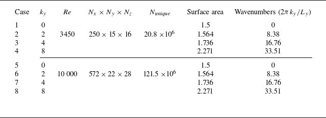


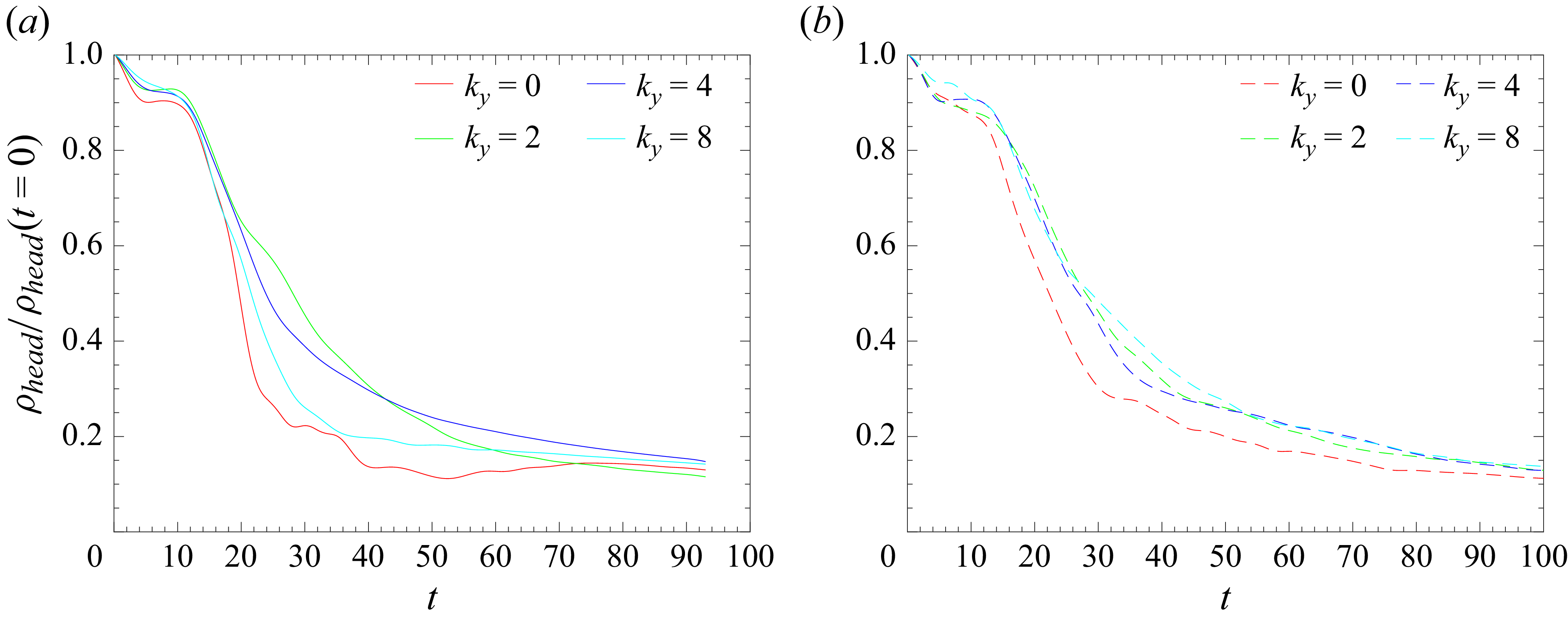


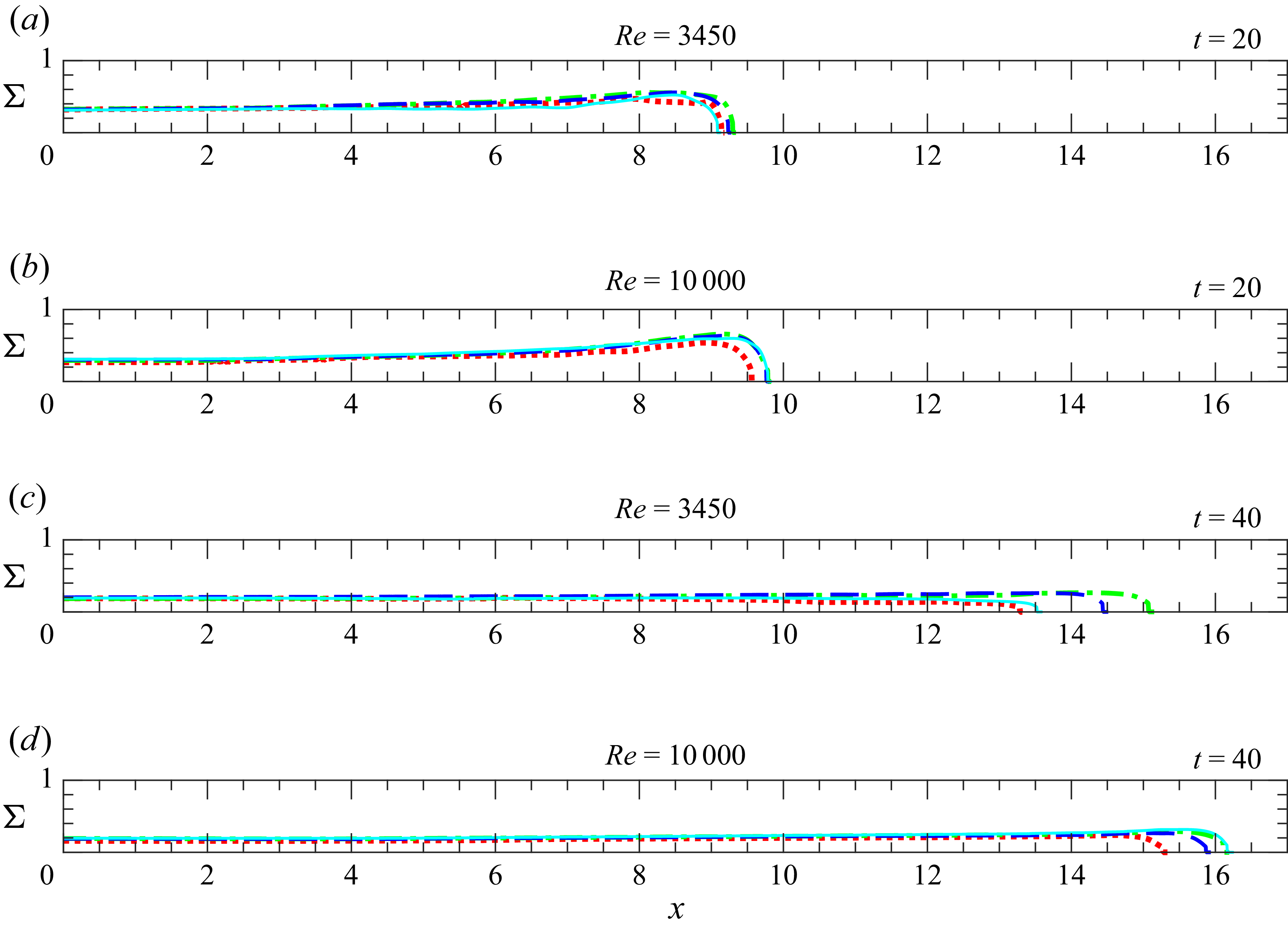


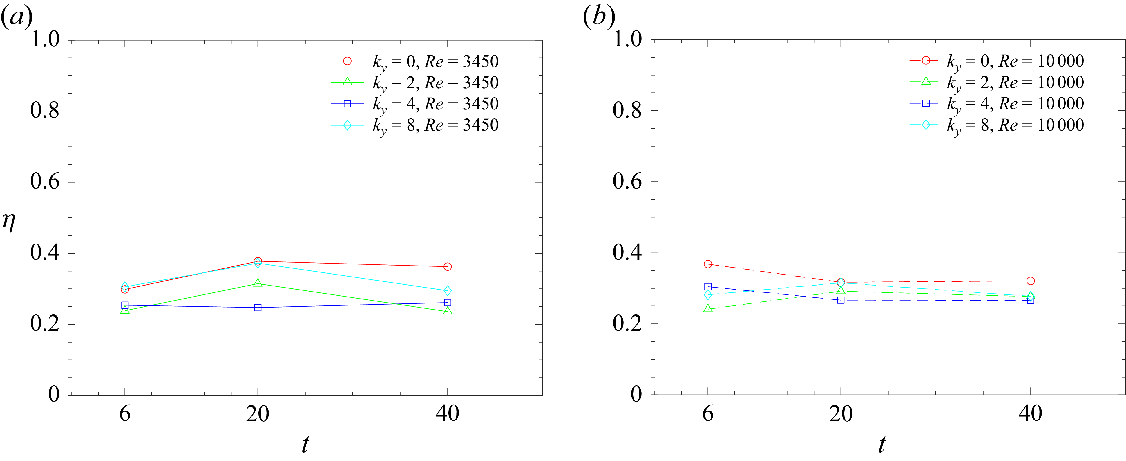


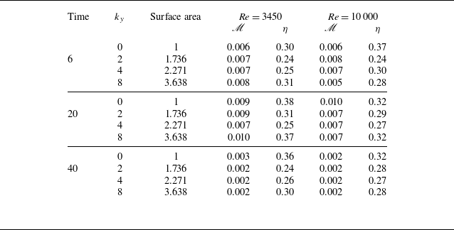


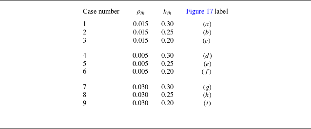


 Open access