2.1. The DSMC algorithm

The particle-based DSMC method (Bird Reference Bird1994) is employed to fully resolve the three-dimensional unsteady hypersonic flow field in question. DSMC is a computationally powerful tool, based on the decoupling of molecular motion and intermolecular collisions, in which each simulated particle represents a finite number, $F_{n}$, of actual gas molecules. When all numerical parameters are satisfied, the time-accurate flow field represents a solution of the Boltzmann equation of transport of the molecular velocity distribution function, $f(t,\boldsymbol {r},\boldsymbol {v})$ with respect to time $t$ and position vector $\boldsymbol {r}$, as

(2.1)\begin{equation} \frac{\partial f}{\partial t} + (\boldsymbol{v} \boldsymbol{\cdot} \boldsymbol{\nabla}) f + \left( \frac{\boldsymbol{F}}{m} \boldsymbol{\cdot} \boldsymbol{\nabla}_v \right)f = \left[\frac{{\rm d}f}{{\rm d}t}\right]_{coll} \end{equation}

where $\boldsymbol {v}$ is the instantaneous velocity vector, m is the mass, and $\boldsymbol {\nabla }$ and $\boldsymbol {\nabla }_v$ are gradient operators in physical and velocity spaces, respectively. The first, second and third terms on the left-hand side describe the change of $f$ with time, convection of molecules in space, and convection in velocity space as a result of the external conservative forces per unit mass $\boldsymbol {F}/m$, such as gravity or electric field, which are ignored in this work, respectively. The right-hand side term accounts for changes in $f$ in an element of space–velocity phase space due to intermolecular collisions. Vincenti & Kruger (Reference Vincenti and Kruger1965) provide a thorough description of the Boltzmann equation.

The DSMC algorithm typically comprises four major steps of particle mapping, selection for collisions, evaluation of collision outcomes and movement. Based on the choice of boundary conditions, particles are introduced, removed or reflected from the domain boundaries and interacted with the embedded surfaces using gas-surface collision models during a timestep. They are then mapped to a mesh that encompasses the flow domain with cell size, $\Delta x$, that is smaller than the local mean free path of molecules, $\lambda$. Particle pairs are selected for collisions based on the appropriate elastic or inelastic collision cross-section and are then assigned post-collisional instantaneous velocities and internal energies in each computational cell. Macroscopic flow quantities of interest such as pressure, velocities and temperature can be derived from the microscopic properties of simulated particles using the statistical relations of kinetic theory. Finally, based on the post-collisional outcome, particles are moved with a timestep, $\Delta t$, that is lower than the local mean collision time, $\tau$. Conveniently, this physics based approach provides accurate modelling of the internal structure of shocks, their mutual interactions and surface rarefaction effects. This warrants the use of DSMC for detailed modelling of shock-wave/boundary-layer interactions (SBLIs), compared with ad hoc techniques of modelling shocks in numerical solutions of the Navier–Stokes equations that fall short of accurately capturing the internal structure of the shock (Liepmann et al. Reference Liepmann, Narasimha and Chahine1962).

However, to obtain a physically meaningful solution of an unsteady SBLI flow, a number of numerical criteria must be satisfied (see Tumuklu et al. Reference Tumuklu, Levin and Theofilis2018a). To overcome this challenge, an octree-based, three-dimensional DSMC solver known as Scalable Unstructured Gas-dynamic Adaptive mesh-Refinement (SUGAR-3D) (see Sawant et al. Reference Sawant, Tumuklu, Jambunathan and Levin2018) has been utilised in the present work. In summary, the code takes advantage of adaptive mesh refinement (AMR) of coarser Cartesian octree cells to achieve spatial fidelity at regions of strong gradients, cutcell algorithms to correctly model gas-surface collisions in the vicinity of embedded surfaces, domain decomposition strategy based on Morton-Z space filling curves and inclusion of thermal non-equilibrium models, all within a message-passing-interface (MPI) environment that enables massively parallel communication. In the octree-based AMR framework, the collision or $C$-mesh is formed from a user-defined, uniform Cartesian grid with cells, known as ‘roots’, that are recursively subdivided into eight parts until the local cell size is smaller than the local mean free path. Note that a subdivision based on the above criterion is performed only if there are at least 32 particles in a collision cell.

The satisfaction of the numerical criteria in the flow over the three-dimensional double wedge depends on the free-stream conditions, given in table 1. Table 2 provides a summary of the key numerical parameters for these simulations which were found to require $\sim$60 billion computational particles and $\sim$4.5 billion collision cells of the adaptively refined $C$-mesh octree grid. Here, the Knudsen number is based on the length of the lower wedge, 50.8 mm, $F_n$ denotes the number of actual gas molecules represented by a computational particle, while the wall surface is fully accommodated (Bird Reference Bird1994), i.e. isothermal. The appendix of Sawant et al. (Reference Sawant, Tumuklu, Theofilis and Levin2022) describes the DSMC numerical criteria and convergence study for flows presented here. Figure 6(b,c) of Sawant et al. (Reference Sawant, Tumuklu, Theofilis and Levin2022) show that the ratio $\tau /\Delta t$ is greater than unity in the entire flow domain and the smallest collision cells contain at least eight particles, respectively. With respect to $\lambda /\Delta x$, figure 6(a) of Sawant et al. (Reference Sawant, Tumuklu, Theofilis and Levin2022) shows that the ratio is greater than unity in the entire flow domain, including the interior zones of shock structures and regions of triple, separation and reattachment points. This ratio is between 0.9 and 1, however, in close proximity to the corner of two wedges, also known as the hinge, inside the recirculation region, where the expected errors in transport coefficients of shear viscosity and thermal conductivity are within 6.2 and 3.7 %, respectively (see Alexander, Garcia & Alder Reference Alexander, Garcia and Alder1998). Finally, figure 6(e) of Sawant et al. (Reference Sawant, Tumuklu, Theofilis and Levin2022) also shows that the effect of doubling the number of particles produced the same transient behaviour, where the instantaneous, spanwise-averaged, streamwise velocity differed by at most 7 % in the small region where $\lambda /\Delta x=0.9$ and by 1.5 % outside of it.

Table 1.

Physical gas parameters.

Table 2.

Numerical simulation parameters.

In terms of collision models, the majorant frequency scheme (MFS) of Ivanov & Rogasinsky (Reference Ivanov and Rogasinsky1988) derived using the Kac stochastic model for the selection of collision pairs and the variable hard sphere model for elastic collisions are used. Appendix A describes an improved strategy for the computations of maximum collision cross-section used in the MFS scheme for accurate spectral analysis of unsteady flows simulated on adaptively refined grids. For rotational relaxation, the Borgnakke & Larsen (Reference Borgnakke and Larsen1975) model is employed with rates of Parker (Reference Parker1959) and DSMC correction factors (see Lumpkin, Haas & Boyd Reference Lumpkin III, Haas and Boyd1991; Gimelshein, Gimelshein & Levin Reference Gimelshein, Gimelshein and Levin2002) that account for the temperature dependence of the rotational probability. For vibrational relaxation, the semi-empirical expression of Millikan & White (Reference Millikan and White1963) is used with the high-temperature correction of Park (Reference Park1984).

2.2. Initialisation of three-dimensional flow

The three-dimensional flow studied in this work is initialised using the two-dimensional steady-state solution over a double wedge simulated by Tumuklu et al. (Reference Tumuklu, Levin and Theofilis2019). The latter flow is recalculated here and then replicated on every octree cell along the spanwise direction ($Y$) to form the three-dimensional field at the beginning of the unsteady simulation. Note that the Cartesian coordinates of streamwise, spanwise, streamwise-normal directions are designated as $X$, $Y$ and $Z$, respectively. From the inlet boundary at $X=0$, an inward-directed local Maxwellian flow is introduced at an average number density, bulk velocity and temperature of $n_1$, $u_{x,1}$ and $T_{tr,1}$, respectively. For this work, the SUGAR solver is employed with spanwise-periodic boundary condition in the $Y$-direction, as described in Appendix A. The spanwise extent of the current simulation is $L_y=28.8$ mm, which will be shown to be sufficiently wide to capture linearly growing spanwise-periodic flow structures. In subsequent sections, contours and isocontours showing the detailed spanwise-periodic structures are presented with two periodic wavelengths for clarity.

In terms of the computational strategy used, it takes $\sim 50T$ (flow-through time, $T$, defined in the next section) until the onset of linear instability. To minimise data storage, we estimate this time at which the spanwise-periodic flow structures start to emerge such that they can be easily detected in the background of statistical fluctuations in DSMC. We use an equilibrium criterion along the lines of Hadjiconstantinou et al. (Reference Hadjiconstantinou, Garcia, Bazant and He2003) to quantify the amount of spanwise fluctuations about the two-dimensional base state. For example, the standard deviation in the bulk velocity at equilibrium can be calculated as, $\sigma _u=\sqrt {R\langle T_{tr}\rangle _s/\langle N\rangle _s}$, where $\langle T_{tr}\rangle _s$ and $\langle N\rangle _s$ are local spanwise-averaged translational temperature and number of particles, respectively, and $R$ is the gas constant. The linear instability can be easily detected, when the DSMC-computed standard deviation is larger than the above criterion.

Finally, to accommodate billions of computational particles and collision cells, 19.2 k MPI processors were used in this simulation. The spanwise-periodic simulation takes $\sim$5.5 h per through-flow time ($T$) using Intel Xeon Platinum 8280 (‘Cascade Lake’) processors of the Frontera supercomputer (2019) and $\sim$14 h per flow time using Intel Xeon Platinum 8160 (‘Skylake’) processors of the Stampede2 supercomputer (2019). The overall cost of the simulation up to $T=190$ discussed in what follows required $\sim$870 k node hours ($\sim$43.8 million core hours) of computing time.

2.3. Main features of the two-dimensional base flow

Starting with the two-dimensional base flow, figure 1(a) shows the complex features of an Edney-IV type SBLI system (Edney Reference Edney1968; Babinsky & Harvey Reference Babinsky and Harvey2011). The base flow results are obtained by spanwise and temporally averaging the DSMC flow fields between $T=48$ and 60, where $T$ is the non-dimensional flow time, defined as the time it takes for the flow to traverse the distance $L_s=40$ mm at a free-stream velocity of $u_{x,1}$; $L_s$ is defined as the straight-line distance from the separation point, $P_s$, to the reattachment point, $P_R$, which mark the origin and end of the shear layer inside the separation bubble, respectively. The SBLI features include the interactions of the separation shock with the leading-edge oblique and detached bow shocks at triple points $T_1$ and $T_2$, respectively. Two contact surfaces, $C_1$ and $C_2$, are formed downstream of triple points $T_1$ and $T_2$, respectively, where $C_1$ is between two supersonic streams downstream of the separation shock, and $C_2$ is between the supersonic and subsonic streams downstream of the separation and detached shocks, respectively. For details about the earlier time evolution of the two-dimensional SBLI features over the double wedge, see Tumuklu et al. (Reference Tumuklu, Levin and Theofilis2019).

Figure 1.

(a) Magnitude of mass density gradient of the base flow, $|\boldsymbol {\nabla }\rho _b|$, normalised by $\rho _1L_s^{-1}$, where $\rho _1=n_1 m$ is free-stream mass density. (b) Overlaid on the image shown in (a) are the wall-normal directions $U$, $S$ and $R$, and the numerical probes $a, b, c, d, r, s$ and $t$, defined in the text.

The image shown in figure 1(a) is repeated in figure 1(b), in order to define a number of probes that will aid the discussion of the next sections. Probes are placed at locations $a$: at the foot of the separation shock, ($X=32.817$ mm, $Z=13.285$ mm), $b$: inside the LSB, ($X=48.496$ mm, $Z=24.270$ mm), $c$: at the contact surface, ($X=65.191$ mm, $Z=56.593$ mm), $d$: on the detached shock, ($X=52.860$ mm, $Z=59.226$ mm), $r$: at reattachment, ($X=64.396$ mm, $Z=44.358$ mm), $s$: on the separation shock, ($X=44.165$ mm, $Z=32.597$ mm) and $t$: at the triple point $T_2$, ($X=48.347$ mm, $Z=41.624$ mm). Probes $a$ and $d$ define lines $a\text {--}t$ and $t\text {--}d$, denoting the intersection with the $OXZ$ plane of two planes passing through the separation and detached shocks, respectively. Wall-normal directions $U$, $S$ and $R$ are respectively defined at the foot of the separation shock and either side of the triple point, $T_2$. The vertical projection of the foot of the arrows $U$, $S$ and $R$ on the X-axis is at 32.5, 49 and 66.1 mm, respectively. From this point onward, the DSMC-derived instantaneous profiles shown are noise filtered using the proper orthogonal decomposition (POD) procedure discussed in Appendix B.

The use of a particle-based approach permits analysis of surface rarefaction effects; results corresponding to the base flow are shown in figure 2(a) for the local streamwise velocity slip, $V_{s}$, normalised by $u_{x,1}$, while the local mean free path adjacent to the wall, $\lambda$, as well as the translational temperature jump at the surface are presented in figure 2(b), respectively normalised by free-stream mean free path $\lambda _1$ and $T_{tr,1}$.

Figure 2.

Surface macroscopic flow quantities in the base state, where the profiles are time averaged from $T=48$ to 53. (a) Surface velocity slip in the local streamwise direction, $V_{s}$. (b) Value of $\lambda$ adjacent to the wall and temperature jump $T_{s}$. (c) The heat transfer and pressure coefficients, $C_h$ and $C_p$, respectively.

Figure 2(a) shows a maximum $V_s$ equal to 2.16 % of $u_{x,1}$ at the leading edge ($X=10$ mm), similar to the value of 2.45 % obtained by Tumuklu et al. (Reference Tumuklu, Levin and Theofilis2019) in a two-dimensional flow simulation. The large slip at the leading edge is due to the increased rarefaction of gas induced by steep gradients of the leading-edge shock. Here, $V_s$ decreases along the local streamwise direction to 0.6 % at $X=32$ mm, similar to the decrease of $\lambda$ adjacent to the wall as seen from figure 2(b). From $X=32$ to 36 mm in the interaction region of the separation shock with the boundary layer, $V_{s}$ rapidly decreases to zero at the separation point, $P_S$. Inside the recirculation zone, from $P_S$ to $P_R$, the point of reattachment, $V_{s}$ is negative because the flow impinging on the wall is opposite to the local streamwise direction; $V_{s}$ and $\lambda$ remain constant on the lower wedge, where the latter is approximately 3.69 % of the free-stream mean free path, $\lambda _1$. On the upper slant surface, $V_{s}$ and $\lambda$ both increase such that the rate of increase is significantly larger downstream of reattachment while $T_s$ follows a similar variation as $V_{s}$ and $\lambda$, as seen from figure 2(b). Velocity slip and temperature jump are rarefaction effects that are proportional to the size of the Knudsen layer in the vicinity of the wall (Chambre & Schaaf Reference Chambre and Schaaf1961; Kogan Reference Kogan1969). Since the Knudsen layer is approximately of the order of $\lambda$, which is inversely proportional to number density, $n$, and directly proportional to the translational temperature, $T_{tr}^{\omega -0.5}$, where $\omega =0.745$ is the viscosity index of the gas, the profiles of $V_s$ and $T_s$ are similar to the profile of $\lambda$ in the vicinity of the surface, for our assumption of a fully diffuse surface.

The variations in surface heat flux and pressure coefficients, $C_h$ and $C_p$, respectively, are shown in figure 2(c). The change in $C_h$ along the local streamwise direction is similar to $V_s$ and $T_s$ and $C_p$ is constant on the lower wedge, except for a sharp increase in the vicinity of the separation point from $X=32$ to 38 mm. Inside the recirculation zone on the lower wedge, $C_p$ plateaus, but on the upper wedge it increases rapidly up to the corner of the wedge. It must be noted that, although figure 2(c) shows a small dip in $C_p$ at the hinge equal to 1.36 % of the plateau at $X\sim 50$ mm, we do not observe secondary vortices in the separation region. This is consistent with the value of the scaled angle $\alpha \sim 2$ of our simulations, which is much smaller than that required for secondary vortices to emerge ($4 \le \alpha \le 5$) (see Shvedchenko Reference Shvedchenko2009). The scaled angle is calculated based on the definition used by Gai & Khraibut (Reference Gai and Khraibut2019) (eq. (1.1)), which was originally defined by Stewartson (Reference Stewartson1970) and Rizzetta et al. (Reference Rizzetta, Burggraf and Jenson1978a).

3.1. Analysis of the three-dimensional DSMC signal

During the early time of the simulation, when deviations from the imposed steady state are still small in magnitude, perturbations $\tilde {Q}$ of an unsteady macroscopic flow quantity $Q = (n,u_x,u_y, u_z, T_{tr}, T_{rot}, T_{vib})^{\text {T}}$ may be obtained by subtracting from the unsteady three-dimensional full DSMC field the steady, two-dimensional base flow state $\bar {Q} = (\bar {n},\bar {u}_x,0, \bar {u}_z, \bar {T}_{tr}, \bar {T}_{rot}, \bar {T}_{vib})^{\text {T}}$ computed in § 2.2 and imposed as initial condition in the simulation

(3.1)\begin{equation} \tilde{Q}(x,y,z,t)=Q(x,y,z,t)-\bar{Q}(x,z). \end{equation}

In the disturbance field vector $\tilde {Q}= (\tilde {n},\tilde {u}_x,\tilde {u}_y, \tilde {u}_z, \tilde {T}_{tr}, \tilde {T}_{rot}, \tilde {T}_{vib})^{\text {T}}$, $\tilde {n}$ denotes the perturbation number density, $\tilde {u}_x,\tilde {u}_y, \tilde {u}_z$ are perturbation velocities in the $X$, $Y$ and $Z$ directions and $\tilde {T}_{tr}, \tilde {T}_{rot}, \tilde {T}_{vib}$ are perturbation translational, rotational and vibrational temperatures, respectively. The smallness of the perturbations at early times in the simulation permits decomposition of the DSMC-computed perturbation flow fields $\tilde {Q}$ according to linear stability theory into a spanwise-independent vector $\hat {Q}(x,z)$, comprising the two-dimensional amplitude functions, and a phase function, $\varTheta$, according to (Theofilis Reference Theofilis2000; Theofilis & Colonius Reference Theofilis and Colonius2003)

(3.2)\begin{equation} \tilde{Q}(x,y,z,t) = \hat{Q}(x,z)\exp{(\text{i}\varTheta)} + \text{c.c.}, \end{equation}

where

(3.3)\begin{equation} \varTheta = \beta y - \varOmega t, \end{equation}

Here, $\beta =2{\rm \pi} /L_y$ is the real spatial wavenumber corresponding to the spanwise wavelength, $L_y$, of the global mode, ${\varOmega =\varOmega _r + \text {i} \varOmega _i}$ is a complex quantity, whose real part, $\varOmega _r$, indicates the frequency and the imaginary part, $\varOmega _i$, is the temporal growth rate and $\text {c.c.}$ indicates complex conjugation so that $\tilde {Q}$ is real. The sign convention in (3.3) indicates that $\varOmega _i>0$ signifies exponentially growing linear perturbations.

3.2. Linear instability in the three-dimensional shock layer/LSB interaction region

Analysis of the DSMC results was performed during two time windows, $30\le T\le 68$ and $68 \le T\le 190$. The lower limit of the first bracket was chosen after initial transients in the solution had subsided, while the upper limit in the second time interval was chosen in order to study the long-time development of the instability, once nonlinear saturation had been reached. A qualitative change that occurs after $T=68$ in the shock structure and its long-time ($T>110$) effect on the LSB will be discussed in § 3.4; in this and the next section an in-depth discussion of the results obtained during the linear growth of perturbations is presented first.

The temporal evolution of the spanwise perturbation velocity component, $\tilde {u}_y$, normalised by $u_{x,1}$, within the time of linear growth, indicated by the greyed out box in figure 3, is presented at probe $s$ inside the shock and probe $b$ inside the LSB, both at two spanwise locations, $C$ and $D$, to be defined shortly. The immediate observation made is that, both inside the shock layer and in the LSB, $\tilde {u}_y$ grows exponentially and, up to this time, monotonically. In order to verify the existence of an underlying linear instability mechanism and quantify its parameters, a two-dimensional linear fit of the full three-dimensional field of the perturbations is performed according to (3.2) using the generalised least-squares method of the Python LMFIT (Version 1.0.1) function. The results returned for the mean value of the unknown fit parameters, $\varOmega _i$, $\hat {Q}$, $\varOmega _r$, alongside the $1\sigma$-uncertainty (standard error) of these estimates, are presented in table 3, where the growth rates obtained for macroscopic flow quantities at probes $b, s, r$ and $c$ defined in figure 1 are shown.

Figure 3.

Temporal evolution of spanwise perturbation velocity, (a) in the separation shock (probe $s$) and (b) the bubble (probe $b$), at spanwise locations $C$ ($y/L_y=0.13$) and $D$ ($y/L_y=0.63$).

Table 3.

Two-dimensional linear curve fit parameters obtained using (3.2) and (3.3). Fit parameters are obtained at probe $b$ unless explicitly indicated otherwise.

The results of curve fits at all locations examined indicate the presence of an amplified stationary global linear instability. The average growth rate of each flow quantity listed in the table is $\varOmega _i=5.0$ kHz, with a standard deviation of $\sim$ 6.7 %. Significantly, the absolute magnitude of the small amplitude of spanwise perturbation velocity, $\tilde {u}_y$, is of the same order at probes $r$, $b$, $s$, and an order of magnitude lower at probe $c$: the maximum deviation of $\sim$11.4 % is found at probe $c$, which is outside of the region of shock and LSB interaction.

The temporal evolution of $\tilde {u}_y$ at $50 \le T \le 90$ over the entire span of the separation bubble is shown in figure 4(a) as raw DSMC data, while figure 4(b) shows a two-dimensional linear fit of the data shown in figure 4(a) using (3.2) and (3.3). A well-defined harmonic pattern of $\tilde {u}_y$ emerges along the span and the choice of points $C$ and $D$ becomes clear, as they represent the spanwise locations at which $\tilde {u}_y$ attains a local maximum and minimum, respectively.

Figure 4.

Temporal evolution of spanwise perturbation velocity, $\tilde {u}_y$, inside the LSB, along the entire span. (a) Raw DSMC data. (b) Two-dimensional linear fit of the result shown in (a).

The emergence of linear instability in the DSMC simulation is demonstrated in figure 5, where the probe results shown in figure 3 at location C are plotted again in semi-logarithmic scale; superposed upon the DSMC results a straight line is plotted, having a slope $\varOmega _i=5.0$ kHz, as indicated by the average value of 5 kHz of the amplification rate calculated earlier. A number of significant conclusions can be drawn on the basis of these results. First, perturbations grow exponentially by at least one order of magnitude inside the separation bubble and the shock layer, up to times $T\approx 110$ and $T\approx 130$ at probes $b$ and $s$, respectively. Second, within the one standard deviation error bar of 0.335 kHz (6.7 %) calculated earlier, growth of perturbations occurs at the same amplification rate inside the bubble and the shock, as indicated by the parallel slopes of the straight dashed line and those of the probe data. Third, at these conditions nonlinear saturation, indicated by the oscillatory evolution of the signal that will be discussed in the next section, occurs first inside the LSB and sets in later in the shock layer.

Figure 5.

Same data at location $C$ as in figure 3, plotted in a semi-logarithmic scale. The dashed line shows the average value of the growth rate shown in table 3, $\varOmega _i\approx 5$ kHz, i.e. $\varOmega _i L_s/u_{x,1}\approx 5.247\times 10^{-2}$. The colour for the data at probe $b$ has been changed to distinguish from the data at probe $s$.

To the best of the authors’ knowledge, this is the first time that (unsteady) DSMC simulations have captured the growth of linear instability in the context of three-dimensional DSMC simulations. The essential qualitative difference between the present three-dimensional and the earlier two-dimensional results of Tumuklu et al. (Reference Tumuklu, Levin and Theofilis2019) is the discovery of unstable three-dimensional perturbations in the three-dimensional configuration, as opposed to the damped eigenmodes in the two-dimensional work, that ultimately led to a steady state being reached in the two-dimensional flow; the present results show that no such steady state exists in the three-dimensional double-wedge flow at these parameters. Notwithstanding differences in Mach number, a comparison of the present results with those of instability analysis in the double wedge by Sidharth et al. (Reference Sidharth, Dwivedi, Candler and Nichols2018), who analysed a Mach 5 hypersonic flow of a calorically perfect gas, reveals that the present non-dimensional, average growth rate $\varOmega _i=0.0057$ (growth rate results are non-dimensionalised by multiplying $\varOmega _i$ by the boundary-layer thickness at separation, $\delta _{99}=3.35$ mm, and dividing by the free-stream velocity downstream of the leading-edge shock, $u_{x,2}=2930.8\,{\rm m}\,{\rm s}^{-1}$, the latter obtained from inviscid shock theory (Anderson Reference Anderson2003) for the observed shock angle of 41$^{\circ }$) is nearly an order of magnitude larger than the $\varOmega _i=7.5\times 10^{-4}$ obtained in the referenced work. This can be explained by the difference in the angles between the upper and lower wedges, which is $\Delta \theta =15^{\circ }$ in the present and $\Delta \theta =8^{\circ }$ in the referenced work and is consistent with the strong destabilising effect of $\Delta \theta$ found by Sidharth et al. (Reference Sidharth, Dwivedi, Candler and Nichols2018), and also known from the related compression ramp flow (e.g. Cao et al. Reference Cao, Hao, Klioutchnikov, Olivier and Wen2021). Finally, linear instability was found not to affect surface flow quantities. Spanwise variations of the streamwise velocity slip and the temperature jump at the wall were found to be negligible during linear growth of disturbances, such that these quantities are the same as the base state profiles shown in figures 2(a) and 2(b), respectively. The spanwise velocity slip (not shown) was also found to be negligibly small with a maximum spanwise variation of only 0.078 % of $u_{x,1}$.

The question of the spatial origin of linear instability and the spanwise periodicity seen in figure 4 is addressed next. Two locations are selected, $U$ and $S$, as shown in figure 1(b), located upstream of the separation shock and in the separation region, respectively. Figure 6(a) shows the variation of the local streamwise velocity, $u_{t,l}$ along the local wall-normal direction, subscript ‘$t$’ standing for the local streamwise (wall-tangential) component of velocity and ‘$l$’ referring to the lower wedge surface, as a function the wall-normal height $H_l$. Figure 6(b) shows the absolute maximum spanwise variation of $u_{t,l}$ during linear perturbation growth, calculated based on the difference in $u_{t,l}$ at two locations, $A$, at $Y/L_y=0.88$ and $B$, at $Y/L_y=1.38$ of the spanwise sinusoidal modulation induced by linear instability; the significance of these locations $A$ and $B$ will be further elucidated in the next section.

Figure 6.

(a) Boundary-layer profiles in the base state along wall-normal directions $U$ and $S$. Local streamwise velocity, $u_{t,l}$ is normalised by $u_{x,1}$, $H_l$ being the distance along the wall-normal direction. (b) The absolute maximum spanwise variation in $u_{t,l}$ along $B$ and $S$.

Common characteristics of the boundary-layer profiles at $U$ and $S$ are the respective non-zero streamwise velocity component at the wall, due to surface rarefaction effects discussed in § 2.3, and the generalised inflection points (GIPs), indicated by open circles. The essential difference between the profiles at the two locations concerns the respective maximum spanwise variation: at $U$, this is only within 0.05 % of $u_{x,1}$, indicating that the flow upstream of the separation shock is essentially two-dimensional. By contrast, at $S$ the maximum spanwise variation peaks at the inflection point, $H_l/L_y=0.113$, where it is equal to 1.8 % of $u_{x,1}$. In addition, a second local maximum of 0.72 % of $u_{x,1}$ is observed inside the separation shock layer at $H_l/L_y=0.40$. Attention is thus turned to correlating this spanwise inhomogeneity inside the shock layer with global instability in the LSB.

3.3. Correlation of linear instability in the shock layer and the LSB

Figures 7(a) and 7(b) present probe data of perturbation quantities along specific wall-normal and spanwise field lines, respectively. It should be stressed here that the flow components shown are representative of all perturbation quantities, all of which exhibit the same qualitative behaviour, but are not shown for brevity. Figure 7(a) shows the variation of the gradient magnitude of the pressure perturbation, $|\boldsymbol {\nabla } \tilde {p}|$, normalised by $p_1L_s^{-1}$ ($p_1$ being the free-stream pressure) as a function of wall-normal distance, $H_l$, along the $S$-direction. Data are shown at the same two spanwise locations, $A$ and $B$, the choice of which will be discussed shortly. The rapid increase of $|\boldsymbol {\nabla } \tilde {p}|$ at $H_l=0.36L_y$ is indicative of the separation shock, inside of which the value of $|\boldsymbol {\nabla } \tilde {p}|$ far exceeds that in the vicinity of the surface. This criterion was used to indicate the separation shock region in figure 6(a). It is worth pointing out here that the measured thickness of the shock layer based on this criterion, $0.083L_y=2.39$ mm, is comparable to the boundary-layer thickness at separation, $\delta _{99}=3.35$ mm.

Figure 7.

(a) Wall-normal probe data for $|\boldsymbol {\nabla } \tilde {p}|$, along direction $S$ as a function of wall-normal height at two spanwise locations $A$ and $B$ defined in the legend. (b) Spanwise probe data for $\tilde {u}_{t,l}$ inside the separation shock at $H_l/L_y=0.4$ on plane $S$.

The choice of spanwise locations $A$ and $B$ can be understood from results shown in figure 7(b). Here, the spanwise variation of $\tilde {u}_{t,l}$ inside the separation shock layer is plotted at a wall-normal height $H_l/L_y=0.4$ along the $S$-direction. It can be clearly seen that the spanwise locations $A$ and $B$ correspond to the trough and peak of a sinusoidal modulation of $\tilde {u}_{t,l}$.

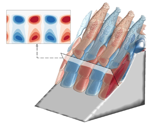
The spanwise structure of small-amplitude perturbations inside the separation and detached shock layers, alongside that inside the LSB, is shown in figures 8(a) and 8(c), respectively corresponding to wall-normal planes at the locations $S$ and $R$ defined in figure 1(b). Figures 8(b) and 8(d) show the same spanwise perturbation velocity component on the separation shock plane $a\text {--}t$ and the detached shock plane $t\text {--}d$ defined in figure 1(b). In all four of these figures contours of the spanwise perturbation velocity component are shown. This quantity is zero at the start of the simulation and only arises on account of linear instability as time progresses. On figures 8(a) and 8(c) the approximate boundaries of the separation and detached shock regions, as well as the envelope of the LSB and the location of the contact surface are marked by dashed/dash-dotted horizontal lines.

Figure 8.

Field data of the spanwise perturbation velocity component, $\tilde {u}_y$, normalised by $u_{x,1}$ during linear growth of perturbations, on the planes $S$ in (a), $a\text {--}t$ in (b), $R$ in (c) and $t\text {--}d$ in (d) as denoted in figure 1(b). Overlaid line contours: (black dashed line) $|\boldsymbol {\nabla } \tilde {p}|$ and (black dashed dotted line) $\tilde {\omega }_y=0$.

On the $S$-plane in figure 8(a), spanwise-periodic flow structures are seen inside the separation bubble between the wedge surface, $H_l=0$, and the outer envelope of the separation bubble, a $H_l\approx 0.15L_y$, where the spanwise vorticity, $\tilde {\omega }_y$, is zero. The outer envelope of the bubble can also be seen to be corrugated sinusoidally, on account of the stationary growing LSB instability, the three-dimensional footprint of which leads to the well-known striations that originate inside the LSB (Ginoux Reference Ginoux1958; Shvedchenko Reference Shvedchenko2009; Dwivedi et al. Reference Dwivedi, Sidharth, Nichols, Candler and Jovanović2019; Hao et al. Reference Hao, Cao, Wen and Olivier2021). This spanwise-periodic global instability is identified here for the first time in the context of kinetic theory simulations.

Further away from the wall, figure 8(a) shows, also for the first time, that spanwise-periodic flow structures form inside the strong gradient region of the separation shock layer, at a height $0.36 < H_l/L_y < 0.44$ away from the wall. These structures are in phase with those inside the LSB and have the same spanwise-periodicity length. This result is consistent with the maximum spanwise variation seen in the probe data and the DSMC signal post-processing discussed in the previous section, which revealed nearly identical growth rates inside the LSB (probe $b$) and the separation shock (probe $s$). The conjecture put forward based on interpretation of the probe data can now be further strengthened on the basis of the field data shown, namely that self-excited linear instability leads to spanwise-periodic structures in perturbation flow quantities within the shock layer, with a spanwise wavelength of $L_y$, identical with that seen in the LSB.

On the cut plane $a\text {--}t$ in figure 8(b), it is seen that the spanwise-periodic structures are present in the entire separation shock layer from the foot of the separation to the triple point $T_2$. The region of interaction of the oblique shock with the separation shock is marked on the $a\text {--}t$ plane at the distance of 0.474$L_y$ to 0.613$L_y$. In this region, the magnitude of $\tilde {u}_y$ increases and striation patterns emerge further along the separation shock.

On the $R$-plane, downstream of the triple point, figure 8(c) shows contour plots of the spanwise perturbation velocity component, $\tilde {u}_y$, which also exhibits spanwise-periodic structures inside the reattached boundary layer; together with the result shown in figure 8(a), this result shows that the striations originating inside the LSB extend at least up to the location of plane $R$ on the downstream wedge wall. Along the wall-normal direction, $H_u$, spanwise-periodic structures are also present in the vicinity of contour line $\tilde {\omega }_y=0$ at a height of $H_u=0.36L_y$, in the vicinity of contact surface $C_2$ downstream of the triple point $T_2$, which clearly points to the contact surface being corrugated by perturbations that are in phase with the striations on the wall. Further away from the wall, the contour lines of $|\boldsymbol {\nabla } \tilde {p}|$ at $H_u=0.61L_y$ and $0.677L_y$ indicate the approximate layer of the detached shock. Inside this layer the spanwise-periodic flow structures are still noticeable, but their amplitude has subsided compared with that in the separation shock, indicating that the spanwise-periodic global mode is concentrated in the zone of interaction between the separation and detached shock-layer system and the LSB.

The presence of spanwise-periodic structures in the detached shock layer from the triple point $T_2$ to probe $d$ is seen on the cut plane $t\text {--}d$ in figure 8(d). The peak magnitude of these structures is at least a factor of two lower than the structures in the separation shock and an order of magnitude lower than those in the separation bubble. This shows that the synchronisation of global instability is strongest between the separation shock and the LSB, and the amplitude of the perturbations in the shock layer declines downstream of the triple point. It can further be seen that the structures inside the detached shock layer are 180$^{\circ }$ out of phase with structures in the separation shock, shown earlier on plane $a\text {--}t$.

Returning to the analysis of the spanwise structures inside the shock layer and the separation bubble on the $S$ plane, figure 9 confirms that spanwise-periodic perturbations are present in all perturbation flow quantities, namely number density, $\tilde {n}$, streamwise velocity with respect to the lower wedge (i.e. direction perpendicular to $S$), $u_{t,l}$, wall-normal velocity with respect to the lower wedge (i.e. direction of $S$), $u_{n,l}$, translational temperature, $\tilde {T}_{tr}$, rotational temperature, $\tilde {T}_{rot}$, and vibrational temperature, $\tilde {T}_{vib}$. The minimum (negative) and maximum (positive) values of spanwise structures in $\tilde {u}_{t,l}$, $\tilde {u}_{n,l}$, and $\tilde {n}$ are also at spanwise locations $A$ and $B$, respectively.

Figure 9.

Contours of perturbation quantities on the plane defined along $S$. (a) Number density, $\tilde {n}$, (b) streamwise perturbation velocity, $u_{t,l}$, (c) wall-normal velocity, $u_{n,l}$, (d) translational temperature, $\tilde {T}_{tr}$, (e) rotational temperature, $\tilde {T}_{rot}$, and ( f) vibrational temperature, $\tilde {T}_{vib}$, showing the cats-eyes pattern of instability in the shock layer. Number density, velocities and temperatures are normalised by respective upstream values.

Interestingly, closer inspection of the relative magnitude of the perturbation velocity components, all scaled by the same free-stream value, reveals qualitatively different results inside the LSB and at the shock layer. In the LSB, the tangential and spanwise perturbation velocity components have comparable magnitudes, while the wall-normal component is an order of magnitude smaller in relative terms. By contrast, the peak oscillation amplitude in the wall-normal perturbation velocity component is two orders of magnitude higher in the shock layer than inside the LSB ($|\tilde {u}_{n,l}|_{max}\approx 0.3$ inside the shock layer, as opposed to $|\tilde {u}_{n,l}|_{max}\approx 3\times 10^{-3}$ in the bubble), as seen in the inset graphs that magnify all shock-layer results. This behaviour, although not as pronounced, can also be seen in the number density and perturbation temperature components.

Furthermore, all three perturbation temperatures have primary spanwise structures adjacent to the wall having minimum and maximum values at spanwise locations $B$ and $A$, respectively, i.e. they are 180$^{\circ }$ out of phase with perturbation structures of velocities and number density. Perturbations in the normalised $\tilde {T}_{tr}$ and $\tilde {T}_{rot}$ also exhibit secondary structures immediately above the primary structures within $0.1 < H_l < 0.15$. From a qualitative point of view, all perturbation components inside the shock layer are found to feature the same cats-eyes pattern, seen in all insets of figure 9. The degree of thermal non-equilibrium seen in the perturbation temperatures presented in figures 9(d)–9( f) is significant, and originates in differences in the base flow temperatures, shown in figure 10(a), where thermal non-equilibrium is present in the entire region between the shock structure and the wedge surface along the three directions shown. This results in the large differences in the shock, denoted by the blue dashed line at $H_l/L_y = 0.36-0.44$ in figure 10(b), where relatively smaller differences can be seen in the bubble, at $H_l/L_y=0-0.15$, in all three temperatures. Consistent with the faster relaxation between translational and rotational modes, those two temperatures have an analogous spatial dependence.

Figure 10.

(a) Base flow temperatures, $\bar {T}_{tr}$, $\bar {T}_{rot}$, $\bar {T}_{vib}$, along $U$, $S$ and $R$. (b) Wall-normal probe data of perturbation temperatures, $\tilde {T}_{tr}$, $\tilde {T}_{rot}$, $\tilde {T}_{vib}$, along $S$ at the spanwise location $A$.

Figure 11 presents three different views of the spanwise perturbation velocity component over the entire calculation domain. In figure 11(a) the perturbation is shown on the $OXZ$ plane and two characteristic cut planes, $P$ and $Q$, defined by their respective normal vectors $[-0.7193\hat {i} + 0.6946\hat {k}]$ and $[0.7193\hat {i} - 0.6946\hat {k}]$. Here, $P$ is taken approximately tangential to the dividing streamline of the LSB, while $Q$ is taken at a distance from the corner, so as to cross the triple point of the steady flow. Figure 11(b) shows three-dimensional isosurfaces of $u_y$ underneath plane $P$, while figure 11(c) presents spanwise-periodic structures in the shear layers downstream of triple points $T_1$ and $T_2$ defined in figure 1(a). All of these results, as well as consistent results seen in the isocontours of vorticity components in Appendix B, all confirm the three-dimensional, spanwise-periodic nature of an instability that encompasses the LSB region in tandem with the separation and detached shock layers and the triple point $T_2$ that connects the latter two.

Figure 11.

(a) Isocontours of spanwise perturbation velocity $\tilde {u}_y$ on the $OXZ$ plane and definition of cut planes $P$ and $Q$. (b) Same result for $\tilde {u}_y$, plotted underneath cut plane $P$ and denoting spanwise-periodic striations inside the LSB. (c) Same plotted upstream of cut plane $Q$ and denoting spanwise-periodic modulation in the vicinity of contact surfaces (shear layers) downstream of triple points.

Summarising, it is seen that during linear perturbation growth the steady two-dimensional base flow becomes unstable to a self-excited, small-amplitude, three-dimensional spanwise-periodic stationary global mode. The spanwise perturbation velocity component, $\tilde {u}_y$, which was zero at the beginning of the simulation, attains a sinusoidally varying amplitude not only inside the separation bubble, as known from earlier work (e.g. Ginoux Reference Ginoux1958; Theofilis et al. Reference Theofilis, Hein and Dallmann2000; Shvedchenko Reference Shvedchenko2009; Dwivedi et al. Reference Dwivedi, Broslawski, Candler and Bowersox2020), but also inside the separation and detached shock layers and the shear layers formed downstream of triple points. This result extends the findings of Tumuklu et al. (Reference Tumuklu, Levin and Theofilis2018a,Reference Tumuklu, Theofilis and Levinb, Reference Tumuklu, Levin and Theofilis2019) in the two-dimensional counterpart of this configuration but, contrary to the two-dimensional limit, in the present three-dimensional environment the observed global instability is unstable with synchronised spanwise-periodic small-amplitude perturbations amplifying exponentially within both the LSB and shock layer. Linear growth of the global mode inside the laminar separation leads to striations on the wall, while in the shock layer a spanwise-periodic cats-eyes pattern is formed in all perturbation components. Ultimately, linear growth will lead to nonlinear saturation and attention is turned next to analysis of the three-dimensional DSMC predictions at later times.

3.4. Low-frequency unsteadiness of the shock and separation bubble

Turning to the dynamics of the linear flow instability at times beyond exponential growth of the stationary spanwise-periodic global mode, attention is paid to low-frequency unsteadiness, that has been reported over a wide range of $Re\sim O(10^{6}-10^{8})$ in a number of numerical solutions of the Navier–Stokes equations (see e.g. Pirozzoli & Grasso Reference Pirozzoli and Grasso2006; Piponniau et al. Reference Piponniau, Dussauge, Debiève and Dupont2009; Touber & Sandham Reference Touber and Sandham2009; Priebe & Martín Reference Priebe and Martín2012; Clemens & Narayanaswamy Reference Clemens and Narayanaswamy2014; Gaitonde Reference Gaitonde2015), as well as many experiments (Dussauge, Dupont & Debiève Reference Dussauge, Dupont and Debiève2006), where shock-induced turbulent boundary-layer interactions were studied in a variety of configurations. Low-frequency unsteadiness is identified in this context as that corresponding to Strouhal numbers in the range $0.01 \le St \le 0.05$, while Strouhal numbers within the same range have also been reported for supersonic laminar and transitional shock/boundary-layer interactions (Sansica, Sandham & Hu Reference Sansica, Sandham and Hu2016; Threadgill, Little & Wernz Reference Threadgill, Little and Wernz2019).

A qualitative change in the evolution of the signal commences in the triple point at $T=68$. Figures 12(a) and 12(b) present the spatio-temporal variation of normalised perturbation spanwise velocity, $\tilde {u}_y$, at probe $b$ in the separation bubble, where linearly growing spatial structures start to exhibit sinusoidal oscillations in time with an average period of 46$T$. At probe $t$ near triple point $T_2$, the variation of normalised perturbation number density, $\tilde {n}$, is shown in figures 12(c) and 12(d) where two time scales with periods of 51$T$ and 41$T$ (average period of 46 $T$) can be seen. The corresponding Strouhal number corresponding to these time periods is,

(3.4)\begin{equation} St = \frac{f L_{s}}{u_{x,2}} = 0.0283 \pm 0.003, \end{equation}

which is defined based on the length of the separation bubble, $L_s=40$ mm and the velocity downstream of the leading-edge oblique shock, $u_{x,2}=2930.8$ m s$^{-1}$. This Strouhal number is within the low-frequency range reported in the literature of turbulent SBLI. The triple point starts to oscillate at $T=68$, and its motion remains two-dimensional up to approximately $T=85$, as indicated by the lack of variation in $\tilde {n}$ along the spanwise direction. Past this time, three-dimensional linear instability manifests itself and low-frequency unsteadiness is observed, causing spanwise modulation of structures in $\tilde {n}$ and their oscillations in time.

Figure 12.

Low-frequency unsteadiness at probes $b$ and $t$ in the separation bubble and at the triple point, $T_2$, respectively. (a) At probe $b$, the temporal evolution of perturbation spanwise velocity, $\tilde {u}_y$, normalised by $u_{x,1}$. (b) At spanwise locations $C$ ($Y/L_y=0.13$) and $D$ ($Y/L_y=0.63$), the normalised $\tilde {u}_y$ indicating the period of unsteadiness (see the greyed out region). (c) At probe $t$, the temporal evolution of perturbation number density, $\tilde {n}$, normalised by $n_1$. (d) Normalised $\tilde {n}$ at locations $A$ ($Y/L_y=0.88$) and $B$ ($Y/L_y=1.38$) as a function of $T$.

In summary, as time progresses, low-frequency oscillation follows exponential growth of a self-excited stationary three-dimensional global mode in the separation bubble and the shock layer. As far as self-excitation of the laminar separation zone is concerned, the appearance of low-frequency oscillation in the related configuration of laminar separation generated by a shock impinging on a flat-plate geometry has been attributed by Boin et al. (Reference Boin, Robinet, Corre and Deniau2006) to a supercritical Hopf bifurcation of the flow, following the oscillator scenario discussed by Theofilis et al. (Reference Theofilis, Hein and Dallmann2000) in the incompressible LSB case.

The present kinetic-theory results fully concur with this prediction regarding the existence of a self-excited three-dimensional stationary global instability of the LSB. Moreover, we find that the underlying global mode is not confined to the LSB but includes the shock layer as an integral part. Past linear amplification of this stationary mode, low-frequency synchronised oscillations arise both in the LSB and in the (fully resolved) shock layer. Current computing capabilities have not permitted us to pursue the time integration of the DSMC equations in order to further quantify additional frequency content generated past the initial stages described herein, or follow flow into transition to turbulence; this task will be pursued in future efforts.