


1. Introduction
Fluvial systems undergo systematic changes in their hydrodynamic response due to ice-jams, logjams at racks and debris accumulation at waste-collection devices (to list a few) as shown in figure 1. In such cases, accumulation of floating materials can induce a transition from a free-surface flow condition to closed-channel-like flow, resulting in complex flow behaviour such as Kelvin–Helmholtz instability and flow separation that depends on the roughness characteristics of the debris at the free surface (Fang, Tachie & Dow Reference Fang, Tachie and Dow2022). Such a change in the boundary condition at the top boundary significantly alters the hydrodynamic response in both the upstream and downstream reaches of the flow domain (Saito & Pullin Reference Saito and Pullin2014; Ismail, Zaki & Durbin Reference Ismail, Zaki and Durbin2018). Specifically, in the vicinity of the transition, the flow encounters significant changes in the mean velocity profile, shear stress and acceleration that can lead to increased turbulent transport, erosion at the bottom boundary and increased instability of the accumulation layer. As a result, understanding the physics of such a flow transition due to the accumulation layer can provide crucial insights to accurately predict its stability and better design hydraulic structures that can efficiently capture floating debris.
Focusing on the formation of a layer of floating material, called a carpet, its life cycle can be divided into the following stages: (i) initiation of accumulation due to the presence of hydraulic structures, (ii) progression due to incoming debris, (iii) stabilisation of the carpet and (iv) mechanical breakup or instability due to unbalanced forces. Depending on the type of debris transported by the incoming flow, carpet formation may consist of one or more layers over the depth of the channel (Shen Reference Shen2010; Schalko et al. Reference Schalko, Schmocker, Weitbrecht and Boes2018; Yan Toe et al. Reference Yan Toe, Uijttewaal and Wüthrich2025). Additionally, surface roughness characteristics of the carpet can differ greatly from those of the channel bed, leading to an asymmetric shear stress distribution as sketched in the downstream reach of the carpet in figure 1. This is typically observed in ice-jams and debris accumulation in rivers (Tatinclaux & Gogus Reference Tatinclaux and Gogus1983; Jueyi et al. Reference Jueyi, Jun, Yun and Faye2010; Luo et al. Reference Luo, Ji, Chen, Liu, Xue and Li2025). Moreover, river morphology is greatly influenced by the surface roughness of ice cover, implying that a larger ratio of ice-cover roughness to bed roughness enhances riverbed erosion (Luo et al. Reference Luo, Ji, Chen, Liu, Xue and Li2025). Moreover, there is still a debate as to whether the location of maximum velocity coincides with the location of zero shear stress in asymmetric channel flows. Hanjalić & Launder (Reference Hanjalić and Launder1972), Tatinclaux & Gogus (Reference Tatinclaux and Gogus1983) and Parthasarathy & Muste (Reference Parthasarathy and Muste1994) confirmed through experimental data that the two locations are not identical. In contrast, Shen & Harden (Reference Shen and Harden1978), Guo et al. (Reference Guo, Shan, Xu, Bai and Zhang2017) and Huai et al. (Reference Huai, Chen, Yang, Li and Wang2024) assumed these locations to coincide in their analyses, leading to the development of two distinct schools of thought. Thus, the momentum flux across the point of zero mean strain ( $\partial \overline {u}_1/\partial x_3=0$
; see figure 1) still remains poorly understood for such a hydraulic system. Therefore, the asymmetry in wall roughness conditions imposes further challenges in correctly estimating the friction coefficients of the boundaries of such hydraulic systems, which are also susceptible to destabilising hydrodynamic forces (Hanjalić & Launder Reference Hanjalić and Launder1972; Guo et al. Reference Guo, Shan, Xu, Bai and Zhang2017; Yan Toe et al. Reference Yan Toe, Uijttewaal and Wüthrich2025).
$\partial \overline {u}_1/\partial x_3=0$
; see figure 1) still remains poorly understood for such a hydraulic system. Therefore, the asymmetry in wall roughness conditions imposes further challenges in correctly estimating the friction coefficients of the boundaries of such hydraulic systems, which are also susceptible to destabilising hydrodynamic forces (Hanjalić & Launder Reference Hanjalić and Launder1972; Guo et al. Reference Guo, Shan, Xu, Bai and Zhang2017; Yan Toe et al. Reference Yan Toe, Uijttewaal and Wüthrich2025).
As for the stability of the carpet, the hydrodynamic forces acting on the debris and interparticle forces determine the threshold mobility, and consequently the overall stability of the carpet. For plastic particles, the hydrodynamic forces affect substantially the global stability of the carpet due to a lack of interparticle cohesion, thus making them susceptible to various instability mechanisms as detailed in Yan Toe et al. (Reference Yan Toe, Uijttewaal and Wüthrich2025). For the ice carpets often observed in ice-jams, Beltaos (Reference Beltaos1983), Zufelt & Ettema (Reference Zufelt and Ettema2000) and Shen, Liu & Chen (Reference Shen, Liu and Chen2001) developed mathematical models to predict the carpet thickness under the static and dynamic flow conditions, assuming a continuum model for ice. Differently from the continuum assumption, Jueyi et al. (Reference Jueyi, Jun, Yun and Faye2010) experimentally investigated incipient motion of individual ice particles under cover and provided a stability criterion, similar to the Shields criterion used in sediment transport. Unlike ice-jams, plastic debris does not interact thermally or through mass transfer (i.e. ice melting), but primarily through hydrodynamic interactions with the carrier phase (i.e. water). Therefore, mechanical properties of the particles and flow conditions are mainly considered in the stability of plastic debris accumulation. In addition to the particle transport at the leading edge of the carpet (called erosion), particles inside the carpet can be squeezed out vertically due to the cumulative compressive force along the carpet (called squeezing), which is similar to the buckling phenomenon observed by Tordesillas & Muthuswamy (Reference Tordesillas and Muthuswamy2009) in force chains. To that end, Yan Toe et al. (Reference Yan Toe, Uijttewaal and Wüthrich2025) developed and validated analytical formulae of these two instability modes, based on the mean flow velocity, particle diameter and particle density in an idealised single-layer carpet of mono-dispersed spherical plastic particles.
Flow transitions from open channel to closed channel. (a) Ice-jam in a river (photo: Bryan Hopkins). (b) Plastic waste accumulation upstream of a waste-collection device (photo: The Ocean Cleanup). (c) Debris jam (Copyright Albert Bridge (image reused under CC Attribution-Sharealike)). (d) Schematic of the flow transition from an open channel to a closed channel (not to scale), based on Yan Toe, Uijttewaal & Wüthrich (Reference Yan Toe, Uijttewaal and Wüthrich2025).

For the squeezing instability, a proper estimate of the cumulative shear stress is required to estimate the destabilising force acting on a particle. Since the flow transitions from an open channel flow to a closed channel with varying hydraulic roughness, estimation of shear stress is non-trivial, especially in the transition region. On this front, Li et al. (Reference Li, De Silva, Rouhi, Baidya, Chung, Marusic and Hutchins2019) and Rouhi, Chung & Hutchins (Reference Rouhi, Chung and Hutchins2019) studied a turbulent boundary layer with roughness transition, and Van Buren et al. (Reference Van Buren, Floryan, Ding, Hellström and Smits2020) studied a turbulent pipe flow with a similar transition, proving that adjustment of turbulent stresses requires a longer downstream fetch than the development length required for the mean flow recovery.
Although there is a substantial literature discussing the boundary-layer development subject to a rough–smooth transition (Antonia & Luxton Reference Antonia and Luxton1971; Van Buren et al. Reference Van Buren, Floryan, Ding, Hellström and Smits2020), the hydrodynamics subject to free slip (open channel) to no slip (closed channel) at the top boundary has not been extensively explored. This is particularly interesting as the boundary layers at the smooth bottom and the rough top interact in the downstream fetch of the carpet, leading to a peculiar flow response in the vicinity of the transition. Adding to the complexity, different roughnesses at the top and bottom boundaries further complicate the momentum mixing and consequently it is more challenging to estimate the friction coefficients. These hydrodynamic interactions hinder the prediction of particle instability, irrespective of the material properties of the particle, i.e. sediment at the riverbed, or plastic particles at the floating carpet. Consequently, in this work, we aim to address the hydrodynamics of an idealised open-to-closed channel transition (figure 1), and its implications for the stability of mono-dispersed spherical particles inside a floating carpet.
To this end, three research questions are formulated as follows:
-
(i) How do the shear stresses and the friction coefficients develop along the bottom and top surfaces beyond the carpet transition?
-
(ii) What changes in the mean flow are observed near the transition?
-
(iii) What are the implications for erosion processes at the bottom boundary and particle instability of debris accumulation?
By better understanding the boundary-layer development at the transition, we aim to further improve the analytical formulations for particle instability, and subsequently better design waste-collection devices and improve river sediment management. It should be noted that the present study considers only mono-dispersed spherical particles as roughness elements, which differ from realistic debris that is more complex in composition, size and shape. For example, plastic waste with cylindrical or foil-like shapes is often found mixed with organic materials, complicating the characterisation of surface roughness. Similarly, large wood accumulations differ in size and shape from spherical elements, with their random orientations leading to a complex porosity within the accumulation layer. Therefore, the flow properties and streamlines, particularly the turbulent stresses near and within the accumulation layer, may differ between the simulation results and realistic configurations. Nevertheless, the present direct numerical simulation (DNS) study is expected to provide valuable insight about mean flow development and Reynolds stress profiles below a generic carpet of debris, waste or ice, and should serve as a baseline for future studies that would address the complex factors described above.
In the following sections, we first present the computational method and various flow configurations to answer the above-mentioned research questions. This is followed by a detailed discussion of the various hydrodynamic parameters of interest. Finally, we present concluding remarks and outline future work to support our analytical model.
2. Methods
The flow configurations investigated in this work are addressed using DNS of the Navier–Stokes equations, coupled with a volume penalisation method (Fadlun et al. Reference Fadlun, Verzicco, Orlandi and Mohd-Yusof2000) to represent a rough carpet layer in the computational domain.
2.1. Governing equations and numerical methods
The differential forms of the incompressible Navier–Stokes momentum and mass conservation equations are considered in this work, given by
 \begin{align} \frac {\partial u_i}{\partial t} + \frac {\partial u_i u_{\kern-1pt j}}{\partial x_{\kern-1pt j}} & = - \frac {1}{\rho } \frac {\partial p}{\partial x_i} + \nu \frac {\partial ^2 u_i}{\partial x_{\kern-1pt j} \partial x_{\kern-1pt j}} + F_i + \varPi \delta _{i1}, \\[-12pt] \nonumber \end{align}
 \begin{align} \frac {\partial u_i}{\partial x_i} & =0, \\[9pt] \nonumber \end{align}
where $t$
is time,
$t$
is time, $x_{\kern-1pt j}$
is the coordinate vector,
$x_{\kern-1pt j}$
is the coordinate vector, $u_i$
are the velocity components,
$u_i$
are the velocity components, $p$
is the pressure,
$p$
is the pressure, $\nu$
is the kinematic viscosity,
$\nu$
is the kinematic viscosity, $\rho$
is the fluid density,
$\rho$
is the fluid density, $F_i$
is the penalisation forcing term, added to the momentum transport equation to enforce the no-slip/no-penetration boundary condition on a particle’s boundary, and
$F_i$
is the penalisation forcing term, added to the momentum transport equation to enforce the no-slip/no-penetration boundary condition on a particle’s boundary, and $\varPi$
is the driving force term used for periodic flow simulations. Kronecker delta
$\varPi$
is the driving force term used for periodic flow simulations. Kronecker delta $\delta _{i1}$
indicates the direction of the driving force term. The penalisation forcing term (Fadlun et al. Reference Fadlun, Verzicco, Orlandi and Mohd-Yusof2000) is calculated as
$\delta _{i1}$
indicates the direction of the driving force term. The penalisation forcing term (Fadlun et al. Reference Fadlun, Verzicco, Orlandi and Mohd-Yusof2000) is calculated as
 \begin{align} F_i = \frac {v_i - u_i}{\Delta t}, \end{align}
where $v_i$
is the velocity imposed at the boundary of the particle (i.e. zero for a stationary object) and
$v_i$
is the velocity imposed at the boundary of the particle (i.e. zero for a stationary object) and $\Delta t$
is the time step used in the simulation. Here, the index
$\Delta t$
is the time step used in the simulation. Here, the index $i=1,\ 2$
and
$i=1,\ 2$
and $3$
denotes the streamwise, spanwise and wall-normal directions, respectively, as sketched in figure 1.
$3$
denotes the streamwise, spanwise and wall-normal directions, respectively, as sketched in figure 1.
The governing equations are spatially discretised using a second-order accurate, finite-difference method over a staggered grid, and integrated in time using a third-order accurate, three-step Runge–Kutta method based on the fractional-step algorithm (Kim & Moin Reference Kim and Moin1985; Costa Reference Costa2018; Ferziger, Perić & Street Reference Ferziger, Perić and Street2019). All the terms in the momentum equation are discretised explicitly and the time integration is performed such that the Courant–Friedrichs–Lewy number does not exceed a value of 0.95. The governing equations are solved using the massively parallel numerical simulation framework CaNS, which has been extensively validated for channel flows at high Reynolds numbers (Costa Reference Costa2018). The computational domain is parallelised using the two-dimensional pencil domain decomposition library developed by Li & Laizet (Reference Li and Laizet2010) and implemented using modern Fortran (Fortran 2004) using the Message-Passing Interface (MPI) for efficient parallel communication over multiple nodes. Additional details of the computational methodology are discussed in Costa (Reference Costa2018) and are not repeated here for brevity.
To introduce a floating carpet composed of individual spheres, an MPI-enabled signed-distance-field (SDF) generator is used (Patil, Paranjothi & García-Sánchez Reference Patil, Paranjothi and García-Sánchez2025), which is based on a geometry-local distance algorithm. All solid objects introduced within the computational domain are identified by correctly masking the negative SDF values that correspond to the inside of the solid object. As for the initial condition, to guarantee rapid development of a turbulent boundary layer for the flow transition simulations (figure 2
f–h), a physical obstacle is placed at the bottom wall to mimic a tripping device traditionally used in experimental facilities. For the simulations with periodic boundary conditions along the streamwise and the spanwise directions, however, a pair of vortices is introduced at the top of the channel that descend downwards to induce turbulence (Perry, Lim & Teh Reference Perry, Lim and Teh1981; Wu Reference Wu2023). A no-slip condition is enforced at the bottom boundary and the top (smooth and rough) boundary, and a free-slip condition is imposed for the free surface assuming the rigid-lid assumption. All data are averaged in time and along the homogeneous directions, respectively, after an initial spin-up time of 10 eddy turnovers ( $T_\epsilon \equiv H/u_{{*b}}$
, where
$T_\epsilon \equiv H/u_{{*b}}$
, where $H$
is the channel height and
$H$
is the channel height and $u_{{*b}}$
is the friction velocity at the smooth bottom boundary) and the results are averaged over a total of
$u_{{*b}}$
is the friction velocity at the smooth bottom boundary) and the results are averaged over a total of $15T_\epsilon$
.
$15T_\epsilon$
.
Various simulation scenarios considered in this work. (a–e) Periodic boundary conditions are employed with a constant bulk velocity $U_{bH}$
, while in (f–h) inflow/outflow conditions are used with a tripping mechanism for a rapid development of the turbulent boundary layer. (a,b,d,e) Auxiliary simulations that are used to compare the flow development of the cases in (f–h). The latter three simulations consider the flow transition from the free-slip to no-slip condition at the top boundary. In further analysis of transition cases TS, TR2 and TR3, the
$U_{bH}$
, while in (f–h) inflow/outflow conditions are used with a tripping mechanism for a rapid development of the turbulent boundary layer. (a,b,d,e) Auxiliary simulations that are used to compare the flow development of the cases in (f–h). The latter three simulations consider the flow transition from the free-slip to no-slip condition at the top boundary. In further analysis of transition cases TS, TR2 and TR3, the $x_1^*=x_1-75H$
coordinate is used for streamwise direction as shown in (f–h).
$x_1^*=x_1-75H$
coordinate is used for streamwise direction as shown in (f–h).

In this work, the flow quantity $\theta$
is decomposed as
$\theta$
is decomposed as
 \begin{align} \theta (x_i,t) = \overline {\theta }(x_i) + \theta '(x_i,t) = \langle \overline {\theta } \rangle (x_3) + \widetilde {\theta }(x_i) + \theta ' (x_i, t), \end{align}
where $\overline {\theta }$
denotes the time-averaged quantity,
$\overline {\theta }$
denotes the time-averaged quantity, $\theta '$
the temporal (turbulent) fluctuation,
$\theta '$
the temporal (turbulent) fluctuation, $\langle \overline {\theta } \rangle$
the time- and plane-averaged quantity and
$\langle \overline {\theta } \rangle$
the time- and plane-averaged quantity and $\widetilde {\theta }$
the dispersive or spatial deviations when compared with the time-averaged quantity
$\widetilde {\theta }$
the dispersive or spatial deviations when compared with the time-averaged quantity $\overline {\theta }$
. For cases where the streamwise and spanwise directions are homogeneous, a periodic boundary condition is applied along these directions (i.e.
$\overline {\theta }$
. For cases where the streamwise and spanwise directions are homogeneous, a periodic boundary condition is applied along these directions (i.e. $x_1$
and
$x_1$
and $x_2$
), thus allowing for the (intrinsic) plane averaging to be performed over these two coordinate directions. For cases where a flow transition is considered, the streamwise direction
$x_2$
), thus allowing for the (intrinsic) plane averaging to be performed over these two coordinate directions. For cases where a flow transition is considered, the streamwise direction $x_1$
is no longer considered homogeneous, and the plane average is performed only over the spanwise direction
$x_1$
is no longer considered homogeneous, and the plane average is performed only over the spanwise direction $x_2$
. However, in the streamwise direction the spatial averaging is performed over a diameter of the spheres in such cases, although the same notation
$x_2$
. However, in the streamwise direction the spatial averaging is performed over a diameter of the spheres in such cases, although the same notation $\langle \theta \rangle$
is used. A detailed explanation of the different simulation scenarios is presented in § 2.2 and figure 2.
$\langle \theta \rangle$
is used. A detailed explanation of the different simulation scenarios is presented in § 2.2 and figure 2.
Numerical simulations corresponding to the illustrations in figure 2. For cases CR2 and CR3, the parameters are normalised by the friction velocity at the smooth bottom boundary $u_{{*b}}$
specific to each case. For cases TR2 and TR3, however, the mesh parameters are normalised by
$u_{{*b}}$
specific to each case. For cases TR2 and TR3, however, the mesh parameters are normalised by $u_{{*b}}$
from cases CR2 and CR3, respectively. In case TS, the flow parameters are normalised by
$u_{{*b}}$
from cases CR2 and CR3, respectively. In case TS, the flow parameters are normalised by $u_{{*b}}$
from case CR2.
$u_{{*b}}$
from case CR2.

The total force acting on the particles is extracted by integrating the penalisation forcing term over the volume of the roughness layer. The force is in turn used to determine the friction velocity at the rough layer $u_{*{t}}$
via
$u_{*{t}}$
via $u_{*{t}} = \sqrt {\langle \overline {\tau }_{{t}} \rangle /\rho }$
(Yuan & Piomelli Reference Yuan and Piomelli2014; Rouhi et al. Reference Rouhi, Chung and Hutchins2019), where
$u_{*{t}} = \sqrt {\langle \overline {\tau }_{{t}} \rangle /\rho }$
(Yuan & Piomelli Reference Yuan and Piomelli2014; Rouhi et al. Reference Rouhi, Chung and Hutchins2019), where $\langle \overline {\tau }_{{t}} \rangle$
is the time- and space-averaged wall shear stress. Alternatively, the wall shear stress can be obtained from the extrapolation of the linear shear stress profile to the bed, though this approach is not applicable to flow transition cases where the fully developed flow is not yet realised. Therefore, in such cases the shear stress
$\langle \overline {\tau }_{{t}} \rangle$
is the time- and space-averaged wall shear stress. Alternatively, the wall shear stress can be obtained from the extrapolation of the linear shear stress profile to the bed, though this approach is not applicable to flow transition cases where the fully developed flow is not yet realised. Therefore, in such cases the shear stress $\langle \overline {\tau }_{{t}}\rangle$
acting on each row of particles within the carpet (denoted as the
$\langle \overline {\tau }_{{t}}\rangle$
acting on each row of particles within the carpet (denoted as the $l{\rm th}$
row for
$l{\rm th}$
row for $l=1,2,3,\dots$
in figure 2
g,h) is calculated by dividing the horizontal component of the averaged penalisation force
$l=1,2,3,\dots$
in figure 2
g,h) is calculated by dividing the horizontal component of the averaged penalisation force $\langle \overline {F}_1 \rangle _l$
acting on that row by the projected area, i.e. the product of the channel width
$\langle \overline {F}_1 \rangle _l$
acting on that row by the projected area, i.e. the product of the channel width $B$
and sphere diameter
$B$
and sphere diameter $d_{{p}}$
.
$d_{{p}}$
.
2.2. Simulation scenarios
To investigate the hydrodynamics of floating carpets under various flow conditions, we consider eight flow configurations as detailed in table 1 and illustrated in figure 2. The first five cases are described as (a) case CS: closed channel flow with both smooth bottom and top boundaries; (b) case OS: open channel flow with a smooth bottom boundary and free surface at the top; (c) case OR: open channel flow with a rough bottom boundary and free surface at the top; (d) case CR2; and (e) case CR3: closed channel with a rough top boundary and a smooth bottom boundary. Case CR2 has a relative roughness given by $d_{{p}}/H = 1/6$
and case CR3 has
$d_{{p}}/H = 1/6$
and case CR3 has $d_{{p}}/H=1/4$
. The aforementioned five cases are intended as the benchmark cases, while case OR is considered to validate the volume penalisation methodology implemented for this study. Case OR corresponds to the F50 configuration in Chan-Braun, García-Villalba & Uhlmann (Reference Chan-Braun, García-Villalba and Uhlmann2011). As presented in Appendix A.1, the comparison between the methodology used in this work and the results in Chan-Braun et al. (Reference Chan-Braun, García-Villalba and Uhlmann2011) shows a good agreement, thus validating the current numerical framework. Details about the validation procedure can be found in Appendix A.1. As for cases CS, OS, CR2 and CR3, flow conditions and geometry parameters are identical to those of the laboratory experiments of Yan Toe et al. (Reference Yan Toe, Uijttewaal and Wüthrich2025). In cases CS, OS, CR2 and CR3, a constant pressure gradient drives the flow such that the bulk Reynolds number
$d_{{p}}/H=1/4$
. The aforementioned five cases are intended as the benchmark cases, while case OR is considered to validate the volume penalisation methodology implemented for this study. Case OR corresponds to the F50 configuration in Chan-Braun, García-Villalba & Uhlmann (Reference Chan-Braun, García-Villalba and Uhlmann2011). As presented in Appendix A.1, the comparison between the methodology used in this work and the results in Chan-Braun et al. (Reference Chan-Braun, García-Villalba and Uhlmann2011) shows a good agreement, thus validating the current numerical framework. Details about the validation procedure can be found in Appendix A.1. As for cases CS, OS, CR2 and CR3, flow conditions and geometry parameters are identical to those of the laboratory experiments of Yan Toe et al. (Reference Yan Toe, Uijttewaal and Wüthrich2025). In cases CS, OS, CR2 and CR3, a constant pressure gradient drives the flow such that the bulk Reynolds number $ \textit{Re}_{bH}=13\,080$
is achieved, where
$ \textit{Re}_{bH}=13\,080$
is achieved, where $ \textit{Re}_{bH}={(U_{bH}\!H)}/{\nu }$
, in which
$ \textit{Re}_{bH}={(U_{bH}\!H)}/{\nu }$
, in which $U_{bH}=(1/H)\int _{0}^H \langle \overline {u}_1 \rangle {\rm d}x_3$
is the bulk velocity based on
$U_{bH}=(1/H)\int _{0}^H \langle \overline {u}_1 \rangle {\rm d}x_3$
is the bulk velocity based on $H$
.
$H$
.
To examine the impact of the transition, three main simulations are considered in this work, namely cases TS, TR2 and TR3 and illustrated in figures 2(f)–2(h), respectively. Case TS is the case with a transition from a smooth open channel to a smooth closed channel. Case TR2 denotes the scenario with a transition from a smooth open channel to a closed channel with a rough top boundary characterised by relatively small roughness ( $d_{{p}}/H=1/6$
). Case TR3 considers a flow configuration similar to that of case TR2 with relatively larger roughness (
$d_{{p}}/H=1/6$
). Case TR3 considers a flow configuration similar to that of case TR2 with relatively larger roughness ( $d_{{p}}/H=1/4$
). In these transition cases TS, TR2 and TR3, a uniform velocity profile is prescribed at the inlet boundary, and the flow develops towards a turbulent boundary layer due to the tripping placed at the bottom wall (see figure 2
f–h). The tripping used in this study consists of a line of hemispheres of diameter
$d_{{p}}/H=1/4$
). In these transition cases TS, TR2 and TR3, a uniform velocity profile is prescribed at the inlet boundary, and the flow develops towards a turbulent boundary layer due to the tripping placed at the bottom wall (see figure 2
f–h). The tripping used in this study consists of a line of hemispheres of diameter $d_{{p}}=0.01$
(
$d_{{p}}=0.01$
( $d_{{p}}/H\approx 0.08$
) placed at
$d_{{p}}/H\approx 0.08$
) placed at $x_1=0.10$
m downstream of the inlet plane. The floating carpet is placed at a distance
$x_1=0.10$
m downstream of the inlet plane. The floating carpet is placed at a distance $x_1/H=75$
away from the inlet boundary to allow a sufficiently long fetch for a fully developed condition. The length of the floating carpet layer
$x_1/H=75$
away from the inlet boundary to allow a sufficiently long fetch for a fully developed condition. The length of the floating carpet layer $\lambda$
is set to
$\lambda$
is set to $\lambda /H = 100/3$
. At the outlet boundary of the flow domain, a Neumann velocity boundary condition is prescribed, while the pressure at the outlet boundary is set to
$\lambda /H = 100/3$
. At the outlet boundary of the flow domain, a Neumann velocity boundary condition is prescribed, while the pressure at the outlet boundary is set to $p = 0$
. It is noted that the current method of imposing a Neumann boundary condition on the streamwise velocity component, combined with the prescribed inflow, naturally imposes the net pressure difference that sustains the flow in this spatially developing channel as in the experiments, whereas this particular combination is not suitable for simulations of a zero-pressure-gradient turbulent boundary layer.
$p = 0$
. It is noted that the current method of imposing a Neumann boundary condition on the streamwise velocity component, combined with the prescribed inflow, naturally imposes the net pressure difference that sustains the flow in this spatially developing channel as in the experiments, whereas this particular combination is not suitable for simulations of a zero-pressure-gradient turbulent boundary layer.
For all rough-channel cases CR2, CR3, TR2 and TR3, the roughness height $k$
is defined as the radius of the individual spherical particles (
$k$
is defined as the radius of the individual spherical particles ( $0.5d_{{p}}$
) of the floating carpet as assumed by Wu, Christensen & Pantano (Reference Wu, Christensen and Pantano2020). Therefore, the relative roughness for cases CR2 and TR2 is
$0.5d_{{p}}$
) of the floating carpet as assumed by Wu, Christensen & Pantano (Reference Wu, Christensen and Pantano2020). Therefore, the relative roughness for cases CR2 and TR2 is $k/H=0.0833$
and for cases CR3 and TR3 is
$k/H=0.0833$
and for cases CR3 and TR3 is $k/H=0.125$
. While the roughness height is known a priori, the equivalent sand grain roughness for large Reynolds number
$k/H=0.125$
. While the roughness height is known a priori, the equivalent sand grain roughness for large Reynolds number $k_{s\infty }$
and the virtual origin
$k_{s\infty }$
and the virtual origin $z_0$
(Nikuradse Reference Nikuradse1933) are derived in Appendix A.2. For some of the cases listed in table 1, the location of the maximum streamwise velocity (
$z_0$
(Nikuradse Reference Nikuradse1933) are derived in Appendix A.2. For some of the cases listed in table 1, the location of the maximum streamwise velocity ( $U_{\textit{max}}$
) is a length scale of interest and, therefore, a friction Reynolds number at the bottom boundary is defined as
$U_{\textit{max}}$
) is a length scale of interest and, therefore, a friction Reynolds number at the bottom boundary is defined as $ \textit{Re}_{{\tau b}} = u_{{*b}} z_m/\nu$
, where
$ \textit{Re}_{{\tau b}} = u_{{*b}} z_m/\nu$
, where $z_m$
is the location of
$z_m$
is the location of $U_{\textit{max}}$
normal to the wall, and a friction Reynolds number at the rough top boundary is defined as
$U_{\textit{max}}$
normal to the wall, and a friction Reynolds number at the rough top boundary is defined as $ \textit{Re}_{{\tau t}} = u_{{*t}} (H-z_m)/\nu$
. In all rough-channel simulations, the spheres are placed in a regular uniform arrangement.
$ \textit{Re}_{{\tau t}} = u_{{*t}} (H-z_m)/\nu$
. In all rough-channel simulations, the spheres are placed in a regular uniform arrangement.
Mean velocity profiles (a) upstream of the transition for all transition cases and (b–d) downstream of the transition for cases TS, TR2 and TR3. The hatched area indicates $\pm 2\,\%$
of velocity profiles of cases OS, CS, CR2 and CR3, respectively. The colourbars mark the positions of the mean velocity profiles along the streamwise direction of the channel with respect to the location of the transition. The red shading in (b) marks
$\pm 2\,\%$
of velocity profiles of cases OS, CS, CR2 and CR3, respectively. The colourbars mark the positions of the mean velocity profiles along the streamwise direction of the channel with respect to the location of the transition. The red shading in (b) marks $\pm \sigma /2$
around the experimental data of Yan Toe et al. (Reference Yan Toe, Uijttewaal and Wüthrich2025) (
$\pm \sigma /2$
around the experimental data of Yan Toe et al. (Reference Yan Toe, Uijttewaal and Wüthrich2025) ( $\sigma$
is the standard deviation). The colourbars indicate the streamwise position with respect to the transition point.
$\sigma$
is the standard deviation). The colourbars indicate the streamwise position with respect to the transition point.

3. Results and discussion
3.1. Streamwise development of global quantities
To analyse the fully developed flow condition as a function of the streamwise distance from the inflow boundary, we discuss the development of the time- and plane-averaged flow parameters, i.e. mean velocity and Reynolds shear stress, for cases TR2 and TR3. These quantities are compared with the results from cases CS, OS, CR2 and CR3 that serve as benchmark datasets.
Figure 3 compares the development of time- and plane-averaged velocity profiles along the streamwise direction of the channel for cases TS, TR2 and TR3. Here the streamwise coordinate origin is set at the start of the floating carpet such that the negative values for the streamwise direction $(x_1-75H)/H\lt 0$
correspond to the flow domain upstream of the carpet, while the positive values for the streamwise direction
$(x_1-75H)/H\lt 0$
correspond to the flow domain upstream of the carpet, while the positive values for the streamwise direction $(x_1 - 75H)/H\gt 0$
correspond to the downstream reach of the carpet. Hereafter,
$(x_1 - 75H)/H\gt 0$
correspond to the downstream reach of the carpet. Hereafter, $(x_1-75H)/H$
will be referred to as
$(x_1-75H)/H$
will be referred to as $x_1^*/H$
, where
$x_1^*/H$
, where $x_1^*=x_1-75H$
, denoted by the colourbars in figure 3. The time- and plane-averaged streamwise velocity profile
$x_1^*=x_1-75H$
, denoted by the colourbars in figure 3. The time- and plane-averaged streamwise velocity profile $\langle \overline {u}_1 \rangle (x_3)$
upstream of the transition in cases TS, TR2 and TR3 is observed to compare well with the profile obtained for the statistically stationary flow of case OS within
$\langle \overline {u}_1 \rangle (x_3)$
upstream of the transition in cases TS, TR2 and TR3 is observed to compare well with the profile obtained for the statistically stationary flow of case OS within $2\,\%$
range of accuracy (figure 3
a). At the transition point
$2\,\%$
range of accuracy (figure 3
a). At the transition point $x_1^*/H=0$
and downstream locations
$x_1^*/H=0$
and downstream locations $x_1^*/H\gt 0$
as shown in figure 3(b–d), the flow encounters a floating carpet and thus undergoes an adaptation to the no-slip boundary condition. In case TS, the velocity profiles do not reach the fully developed velocity profile when compared with the benchmark profile of case CS (figure 3
b). In contrast, case TR2 (figure 3
c) and case TR3 (figure 3
d) exhibit a fully developed flow condition at
$x_1^*/H\gt 0$
as shown in figure 3(b–d), the flow encounters a floating carpet and thus undergoes an adaptation to the no-slip boundary condition. In case TS, the velocity profiles do not reach the fully developed velocity profile when compared with the benchmark profile of case CS (figure 3
b). In contrast, case TR2 (figure 3
c) and case TR3 (figure 3
d) exhibit a fully developed flow condition at $x_1^*/H \approx 33$
. The benchmark results from cases CS, CR2 and CR3 are also shown in figure 3(b–d).
$x_1^*/H \approx 33$
. The benchmark results from cases CS, CR2 and CR3 are also shown in figure 3(b–d).
Comparison of mean velocity profiles normalised by inner scaling: (a) comparison in the vicinity of the physical tripping, (b) comparison upstream of the transition, (c) comparison in the lower half of the channel for case TS, (d) comparison for the upper half of the channel where the debris accumulates, (e) comparison for the bottom half of the channel for case TR2 after the transition and (f) comparison for the upper half of the channel for case TR2 after the transition. In cases TS and TR2, the velocity profiles under the carpet are divided based on the location of the maximum streamwise velocity $z_m$
. Since velocity profiles of case TR3 do not show any significant difference from those of case TR2, results of case TR3 are omitted.
$z_m$
. Since velocity profiles of case TR3 do not show any significant difference from those of case TR2, results of case TR3 are omitted.

To investigate the flow behaviour in the near-wall region, the above-mentioned velocity profiles are plotted again using the viscous length scale or wall unit in figure 4. In all subfigures, the velocity profiles are shifted by $\Delta U^+=5$
for clear visualisation. Figure 4(a) shows the evolution of the flow immediately downstream of the tripping mechanism, and the logarithmic profile is recovered at
$\Delta U^+=5$
for clear visualisation. Figure 4(a) shows the evolution of the flow immediately downstream of the tripping mechanism, and the logarithmic profile is recovered at $x_1^*/H=-40$
. The development of flow profiles upstream of the transition point is depicted in figure 4(b), showing that the approach flow to the carpet compares well against the logarithmic mean velocity profile. To study the velocity profiles in the closed channel region of cases TS and TR2, the profiles are divided based on the location of maximum streamwise velocity, and shown separately in figure 4(c–f). For the rough-channel case TR2, the velocity profiles in the top part need to be shifted for their virtual origins where the logarithmic velocity profile begins, which is further elaborated in Appendix A.2, in figure 4(f). The velocity profiles in all cases are observed to recover at
$x_1^*/H=-40$
. The development of flow profiles upstream of the transition point is depicted in figure 4(b), showing that the approach flow to the carpet compares well against the logarithmic mean velocity profile. To study the velocity profiles in the closed channel region of cases TS and TR2, the profiles are divided based on the location of maximum streamwise velocity, and shown separately in figure 4(c–f). For the rough-channel case TR2, the velocity profiles in the top part need to be shifted for their virtual origins where the logarithmic velocity profile begins, which is further elaborated in Appendix A.2, in figure 4(f). The velocity profiles in all cases are observed to recover at $x_1^*/H=30$
and agree with benchmark results. Since the velocity profiles of case TR3 show shapes similar to those of case TR2, the results of case TR3 are omitted here.
$x_1^*/H=30$
and agree with benchmark results. Since the velocity profiles of case TR3 show shapes similar to those of case TR2, the results of case TR3 are omitted here.
A rapid recovery of first-order statistics, i.e. mean streamwise velocity, is observed in the rough transition cases TR2 and TR3 due to the additional momentum mixing induced by the spheres of the rough carpet. However, in the smooth transition case TS, the first-order statistics cannot be recovered immediately downstream of the transition. Moreover, the simulation results of cases CR2 and TR2 show a good comparison with the experimental result from Yan Toe et al. (Reference Yan Toe, Uijttewaal and Wüthrich2025) in the fully developed condition, except for a slight deviation near the top rough wall (figure 3
c). It should be noted that the laboratory experiments used spheres with a slightly higher submergence of $87\,\%$
.
$87\,\%$
.
Reynolds shear stress profiles for case TR2: (a) upstream of the flow transition and (b) downstream of the transition. The colourbars mark the positions of the Reynolds shear stress profiles along the streamwise direction of the channel with respect to the location of the transition. Since the streamwise position $x_1^*/H\approx 36$
is beyond the end of the carpet and the flow transitions to open-channel flow again (figure 2
g), the stress profile does not follow the benchmark profile.
$x_1^*/H\approx 36$
is beyond the end of the carpet and the flow transitions to open-channel flow again (figure 2
g), the stress profile does not follow the benchmark profile.

The streamwise evolution of the Reynolds shear stress profile for case TR2 is compared against the benchmark cases OS and CR2 in figures 5(a) and 5(b), respectively. Upstream of the transition, the Reynolds stress profiles for cases TR2 and OS are observed to be in good agreement (figure 5
a), whereas the profiles under the carpet in figure 5(b) fail to recover to the linear stress profile observed for the benchmark case CR2. It is noted that at $x_1^*/H \approx -1$
, which is very close to the transition point, the flow already experiences the step change and consequently the profile near the bottom boundary does not agree exactly with the benchmark velocity profile of case OS (figure 5
a). Similarly, since the streamwise position
$x_1^*/H \approx -1$
, which is very close to the transition point, the flow already experiences the step change and consequently the profile near the bottom boundary does not agree exactly with the benchmark velocity profile of case OS (figure 5
a). Similarly, since the streamwise position $x_1^*/H\approx 36$
represents the location downstream of the end of the carpet, the flow transitions again to the open channel flow (denoted as free-slip boundary condition in figure 2
g) and the stress profile is found to deviate from the benchmark case CR2 in figure 5(b). The relatively slow response of the Reynolds stress under the carpet follows the trends previously observed by Rouhi et al. (Reference Rouhi, Chung and Hutchins2019) and Van Buren et al. (Reference Van Buren, Floryan, Ding, Hellström and Smits2020). A similar trend was seen for case TR3, which is not shown here for brevity. There are, however, some minor differences observed closer to the bottom wall when comparing the numerical and the experimental results, which can be presumably attributed to the experimental measurement limitations and additional sidewall effects of the flume. Overall, both the time- and plane-averaged mean flow response and the Reynolds stress profile compare well with the benchmark cases, suggesting that the approach flow conditions upstream of the transition are fully developed in cases TS, TR2 and TR3. Moreover, larger shear stresses are observed near the rough top boundary compared with those near the bottom boundary downstream of the transition point because of roughness-induced turbulence stresses. It is noted that variations in debris size and shape can lead to different observations of the stress distribution.
$x_1^*/H\approx 36$
represents the location downstream of the end of the carpet, the flow transitions again to the open channel flow (denoted as free-slip boundary condition in figure 2
g) and the stress profile is found to deviate from the benchmark case CR2 in figure 5(b). The relatively slow response of the Reynolds stress under the carpet follows the trends previously observed by Rouhi et al. (Reference Rouhi, Chung and Hutchins2019) and Van Buren et al. (Reference Van Buren, Floryan, Ding, Hellström and Smits2020). A similar trend was seen for case TR3, which is not shown here for brevity. There are, however, some minor differences observed closer to the bottom wall when comparing the numerical and the experimental results, which can be presumably attributed to the experimental measurement limitations and additional sidewall effects of the flume. Overall, both the time- and plane-averaged mean flow response and the Reynolds stress profile compare well with the benchmark cases, suggesting that the approach flow conditions upstream of the transition are fully developed in cases TS, TR2 and TR3. Moreover, larger shear stresses are observed near the rough top boundary compared with those near the bottom boundary downstream of the transition point because of roughness-induced turbulence stresses. It is noted that variations in debris size and shape can lead to different observations of the stress distribution.
Streamwise development of turbulent normal stresses $\langle \overline {u_i' u_i'} \rangle$
is also investigated using inner scaling and outer scaling in figures 6(a–c) and 6(d–f), respectively, for case TR2. The profiles are found to approach the benchmark results gradually as expected. As reported by Burattini et al. (Reference Burattini, Leonardi, Orlandi and Antonia2008), the normal stress profiles also show an asymmetric shape in the rough–smooth closed channel due to the different roughnesses. Detailed study of turbulent normal stresses is presented in Appendix A.3 for cases TS and TR3, including the development of the profiles at the inflow section, downstream of the tripping point.
$\langle \overline {u_i' u_i'} \rangle$
is also investigated using inner scaling and outer scaling in figures 6(a–c) and 6(d–f), respectively, for case TR2. The profiles are found to approach the benchmark results gradually as expected. As reported by Burattini et al. (Reference Burattini, Leonardi, Orlandi and Antonia2008), the normal stress profiles also show an asymmetric shape in the rough–smooth closed channel due to the different roughnesses. Detailed study of turbulent normal stresses is presented in Appendix A.3 for cases TS and TR3, including the development of the profiles at the inflow section, downstream of the tripping point.
Vertical profiles of turbulent normal stresses $\langle \overline {u_i' u_i'} \rangle$
downstream of the transition point
$\langle \overline {u_i' u_i'} \rangle$
downstream of the transition point $x_1^*/H\gt 0$
: (a–c) using inner scaling and (d–f) using outer scaling. Yellow-coloured areas in (d–f) indicate the height of the roughness.
$x_1^*/H\gt 0$
: (a–c) using inner scaling and (d–f) using outer scaling. Yellow-coloured areas in (d–f) indicate the height of the roughness.

Development of top boundary layer $\delta ^{{t}}$
, displacement thickness
$\delta ^{{t}}$
, displacement thickness $\delta _*^{{t}}$
and momentum thickness
$\delta _*^{{t}}$
and momentum thickness $\varTheta ^{{t}}$
: (a,c,e) near the transition (zoom-in view for the horizontal dimension) and (b,d,f) under the carpet for cases (a,b) TS, (c,d) TR2 and (e,f) TR3. Yellow regions represent the floating carpet (not to scale).
$\varTheta ^{{t}}$
: (a,c,e) near the transition (zoom-in view for the horizontal dimension) and (b,d,f) under the carpet for cases (a,b) TS, (c,d) TR2 and (e,f) TR3. Yellow regions represent the floating carpet (not to scale).

To study the impact of the floating carpet on the bulk flow, we consider three different metrics that quantify the boundary-layer development: the displacement thickness ( $\delta _*^{{t}}$
) given by
$\delta _*^{{t}}$
) given by
 \begin{align} \delta _*^{{t}} = \int _0^{z_{m}} \left ( 1- \frac {\langle \overline {u}_1\rangle }{U_{\textit{max}}} \right ) \mathrm{d}x_3, \end{align}
the momentum thickness ( $\varTheta ^{{t}}$
) given by
$\varTheta ^{{t}}$
) given by
 \begin{align} \varTheta ^{{t}} = \int _0^{z_{m}} \frac {\langle \overline {u}_1\rangle }{U_{\textit{max}}} \left (1-\frac {\langle \overline {u}_1 \rangle }{U_{\textit{max}}} \right ) \mathrm{d}x_3 \end{align}
and the top boundary layer ( $\delta ^{{t}} \equiv z_m$
) defined as the distance from the wall where the streamwise velocity has a maximum value (
$\delta ^{{t}} \equiv z_m$
) defined as the distance from the wall where the streamwise velocity has a maximum value ( $U_{\textit{max}}$
). Figure 7 compares the above-mentioned metrics for the boundary-layer growth under the floating carpet for cases TS, TR2 and TR3. As the flow approaches the floating carpet, the mean flow is observed to experience the effect of the carpet even in the upstream region as indicated by
$U_{\textit{max}}$
). Figure 7 compares the above-mentioned metrics for the boundary-layer growth under the floating carpet for cases TS, TR2 and TR3. As the flow approaches the floating carpet, the mean flow is observed to experience the effect of the carpet even in the upstream region as indicated by $\delta ^{{t}}$
(figure 7
a,c,e). A more pronounced effect is observed in the case of the rough carpet (figure 7
c,e), whereas a smaller effect is seen in the smooth transition case TS (figure 7
a). Subsequently, the mean flow deflects with a vertically downward flow as shown in figure 17. For case TR2, the top boundary layer (red dashed-dot line in figure 7
d) extends from the top wall to the vertical position of
$\delta ^{{t}}$
(figure 7
a,c,e). A more pronounced effect is observed in the case of the rough carpet (figure 7
c,e), whereas a smaller effect is seen in the smooth transition case TS (figure 7
a). Subsequently, the mean flow deflects with a vertically downward flow as shown in figure 17. For case TR2, the top boundary layer (red dashed-dot line in figure 7
d) extends from the top wall to the vertical position of $(H-\delta ^{{t}})/H \approx 0.4$
and asymptotes to a constant value along the streamwise direction at
$(H-\delta ^{{t}})/H \approx 0.4$
and asymptotes to a constant value along the streamwise direction at $x_1^*/H\geqslant 30$
, suggesting a fully developed flow condition underneath the carpet. The momentum thickness
$x_1^*/H\geqslant 30$
, suggesting a fully developed flow condition underneath the carpet. The momentum thickness $\varTheta ^{{t}}$
and the displacement thickness
$\varTheta ^{{t}}$
and the displacement thickness $\delta _*^{{t}}$
are observed to be relatively smaller compared with
$\delta _*^{{t}}$
are observed to be relatively smaller compared with $\delta ^{{t}}$
as expected. Comparing the boundary-layer growths across cases TS, TR2 and TR3, the relatively larger roughness height in case TR3 induces a larger boundary-layer thickness (figure 7
f), while a smaller boundary layer is observed in the smooth carpet case TS (figure 7
b) for all the metrics discussed above. This is especially true when comparing the asymptotic behaviour where case TR2 is observed to attain a value of
$\delta ^{{t}}$
as expected. Comparing the boundary-layer growths across cases TS, TR2 and TR3, the relatively larger roughness height in case TR3 induces a larger boundary-layer thickness (figure 7
f), while a smaller boundary layer is observed in the smooth carpet case TS (figure 7
b) for all the metrics discussed above. This is especially true when comparing the asymptotic behaviour where case TR2 is observed to attain a value of $(H-\delta ^{{t}})/H \approx 0.4$
, while case TS attains a smaller value of
$(H-\delta ^{{t}})/H \approx 0.4$
, while case TS attains a smaller value of $(H-\delta ^{{t}})/H\approx 0.6$
and case TR3 attains a slightly larger value of
$(H-\delta ^{{t}})/H\approx 0.6$
and case TR3 attains a slightly larger value of $(H-\delta ^{{t}})/H \lt 0.4$
(here smaller values mean a deeper top boundary layer), thus clearly illustrating the impact of the relative roughness height.
$(H-\delta ^{{t}})/H \lt 0.4$
(here smaller values mean a deeper top boundary layer), thus clearly illustrating the impact of the relative roughness height.
We also quantify the relative development of $\delta ^{{t}}$
with respect to the asymptotic value
$\delta ^{{t}}$
with respect to the asymptotic value $\delta ^{{t}}_\infty$
that is obtained from the corresponding benchmark cases, giving the ratio
$\delta ^{{t}}_\infty$
that is obtained from the corresponding benchmark cases, giving the ratio $\| \delta ^{{t}} - \delta ^{{t}}_\infty \|/\delta ^{{t}}_\infty$
as shown in figure 8. All cases TS, TR2 and TR3 exhibit a similar relative growth of
$\| \delta ^{{t}} - \delta ^{{t}}_\infty \|/\delta ^{{t}}_\infty$
as shown in figure 8. All cases TS, TR2 and TR3 exhibit a similar relative growth of $\delta ^{{t}}$
although the shape of case TS differs slightly from that of cases TR2 and TR3, which share an identical shape. Therefore, different roughness heights do not affect the relative growth rate of the boundary layer,
$\delta ^{{t}}$
although the shape of case TS differs slightly from that of cases TR2 and TR3, which share an identical shape. Therefore, different roughness heights do not affect the relative growth rate of the boundary layer, $\| \delta ^{{t}} - \delta ^{{t}}_\infty \|/\delta ^{{t}}_\infty$
.
$\| \delta ^{{t}} - \delta ^{{t}}_\infty \|/\delta ^{{t}}_\infty$
.
Relative development of top boundary layer $\delta ^{{t}}$
with respect to its asymptotic value
$\delta ^{{t}}$
with respect to its asymptotic value $\delta ^{{t}}_\infty$
. The asymptotic value is obtained from the corresponding periodic benchmark cases.
$\delta ^{{t}}_\infty$
. The asymptotic value is obtained from the corresponding periodic benchmark cases.

Similar to a conventional smooth boundary layer, the displacement thickness $\delta ^{*{t}}$
and the momentum thickness
$\delta ^{*{t}}$
and the momentum thickness $\varTheta ^{{t}}$
are smaller than the boundary-layer thickness
$\varTheta ^{{t}}$
are smaller than the boundary-layer thickness $\delta ^{{t}}$
in all transition cases TS, TR2 and TR3. At the location of the fully developed flow in case TR2, their ratios are found to be
$\delta ^{{t}}$
in all transition cases TS, TR2 and TR3. At the location of the fully developed flow in case TR2, their ratios are found to be $\delta ^{{t}}/\delta _*^{{t}}=3.8$
and
$\delta ^{{t}}/\delta _*^{{t}}=3.8$
and $\delta ^{{t}}/\varTheta ^{{t}}=9.6$
, respectively. The momentum thickness is observed within the roughness layer (figure 7
d), meaning that the loss of momentum in the rough boundary layer occurs mostly inside the roughness elements. In case TR3, the thicknesses of the aforementioned three layers (
$\delta ^{{t}}/\varTheta ^{{t}}=9.6$
, respectively. The momentum thickness is observed within the roughness layer (figure 7
d), meaning that the loss of momentum in the rough boundary layer occurs mostly inside the roughness elements. In case TR3, the thicknesses of the aforementioned three layers ( $\delta ^{{t}},\ \delta _*^{{t}}$
and
$\delta ^{{t}},\ \delta _*^{{t}}$
and $\varTheta ^{{t}}$
) are found to be larger than those in case TR2 because the larger roughness pushes the mass and momentum mixing layers further away. Nevertheless, the ratios
$\varTheta ^{{t}}$
) are found to be larger than those in case TR2 because the larger roughness pushes the mass and momentum mixing layers further away. Nevertheless, the ratios $\delta ^{{t}}/\delta _*^{{t}}=3.3$
and
$\delta ^{{t}}/\delta _*^{{t}}=3.3$
and $\delta ^{{t}}/\varTheta ^{{t}}=9.8$
are found in case TR3, which are approximately similar to those observed in case TR2.
$\delta ^{{t}}/\varTheta ^{{t}}=9.8$
are found in case TR3, which are approximately similar to those observed in case TR2.
In addition to the study of boundary-layer thickness, we examined the internal boundary layer (IBL) $\delta _{\textit{IBL}}$
and internal equilibrium layer (IEL)
$\delta _{\textit{IBL}}$
and internal equilibrium layer (IEL) $\delta _{\textit{IEL}}$
which show the immediate response of the flow to changes in the boundary roughness. The layer to which the effect of the new boundary roughness reaches is defined as the IBL, and the lower part of the IBL which obtains a new equilibrium with the new surface is called the IEL (Rouhi et al. Reference Rouhi, Chung and Hutchins2019). Previous work of Rouhi et al. (Reference Rouhi, Chung and Hutchins2019) is referred to for detailed explanation and calculation method of
$\delta _{\textit{IEL}}$
which show the immediate response of the flow to changes in the boundary roughness. The layer to which the effect of the new boundary roughness reaches is defined as the IBL, and the lower part of the IBL which obtains a new equilibrium with the new surface is called the IEL (Rouhi et al. Reference Rouhi, Chung and Hutchins2019). Previous work of Rouhi et al. (Reference Rouhi, Chung and Hutchins2019) is referred to for detailed explanation and calculation method of $\delta _{\textit{IBL}}$
that we apply here. In brief, the slope curve
$\delta _{\textit{IBL}}$
that we apply here. In brief, the slope curve $\mathrm{d}U^+/\mathrm{d}\ln {x_3^+}$
is plotted for each
$\mathrm{d}U^+/\mathrm{d}\ln {x_3^+}$
is plotted for each $x_1$
position as shown in figure 9, and two successive local extrema of the slope curve are identified. Then, two linear fits are applied to the velocity profile in the semi-log scale corresponding to these extrema, and the intersection point of the two fitted lines is determined. This intersection defines the position of
$x_1$
position as shown in figure 9, and two successive local extrema of the slope curve are identified. Then, two linear fits are applied to the velocity profile in the semi-log scale corresponding to these extrema, and the intersection point of the two fitted lines is determined. This intersection defines the position of $\delta _{\textit{IBL}}$
. Here
$\delta _{\textit{IBL}}$
. Here $\delta _{\textit{IEL}}$
is obtained by locating the vertical position corresponding to the first logarithmic region in a composite velocity profile consisting of several individual profiles (Savelyev & Taylor Reference Savelyev and Taylor2005). Figure 9 shows
$\delta _{\textit{IEL}}$
is obtained by locating the vertical position corresponding to the first logarithmic region in a composite velocity profile consisting of several individual profiles (Savelyev & Taylor Reference Savelyev and Taylor2005). Figure 9 shows $\delta _{\textit{IBL}}$
and
$\delta _{\textit{IBL}}$
and $\delta _{\textit{IEL}}$
at the rough top surface for cases TR2 and TR3. Both internal layers (
$\delta _{\textit{IEL}}$
at the rough top surface for cases TR2 and TR3. Both internal layers ( $\delta _{\textit{IBL}}$
and
$\delta _{\textit{IBL}}$
and $\delta _{\textit{IEL}}$
) are found to be almost identical, and inside the external top boundary layer
$\delta _{\textit{IEL}}$
) are found to be almost identical, and inside the external top boundary layer $\delta ^{{t}}$
of the rough surface as observed in the work of Rouhi et al. (Reference Rouhi, Chung and Hutchins2019). Some noise is observed in case TR2 which may be attributed to the sensitivity of the slope-finding method. The green line in figure 9 denotes a power-law fitted line,
$\delta ^{{t}}$
of the rough surface as observed in the work of Rouhi et al. (Reference Rouhi, Chung and Hutchins2019). Some noise is observed in case TR2 which may be attributed to the sensitivity of the slope-finding method. The green line in figure 9 denotes a power-law fitted line, $\delta _{\textit{IBL}} \propto (x_1^*)^\alpha$
as suggested by Li et al. (Reference Li, de Silva, Chung, Pullin, Marusic and Hutchins2022), for
$\delta _{\textit{IBL}} \propto (x_1^*)^\alpha$
as suggested by Li et al. (Reference Li, de Silva, Chung, Pullin, Marusic and Hutchins2022), for $\delta _{\textit{IBL}}$
to estimate its growth rate, and it is found that
$\delta _{\textit{IBL}}$
to estimate its growth rate, and it is found that $\delta _{\textit{IBL}}$
varies as
$\delta _{\textit{IBL}}$
varies as $(x_1^*)^{0.67}$
in case TR2 and varies as
$(x_1^*)^{0.67}$
in case TR2 and varies as $(x_1^*)^{0.38}$
in case TR3. The observed
$(x_1^*)^{0.38}$
in case TR3. The observed $\alpha$
values lie within 0.22 and 0.886 as reported by Rouhi et al. (Reference Rouhi, Chung and Hutchins2019). It should be noted that previous studies on step changes (Antonia & Luxton Reference Antonia and Luxton1971; Li et al. Reference Li, De Silva, Rouhi, Baidya, Chung, Marusic and Hutchins2019; Rouhi et al. Reference Rouhi, Chung and Hutchins2019) did not consider the influence of the bottom boundary, but here the presence of the smooth bottom boundary is incorporated in the DNS study of rough boundary-layer development, creating a closed and asymmetric flow geometry.
$\alpha$
values lie within 0.22 and 0.886 as reported by Rouhi et al. (Reference Rouhi, Chung and Hutchins2019). It should be noted that previous studies on step changes (Antonia & Luxton Reference Antonia and Luxton1971; Li et al. Reference Li, De Silva, Rouhi, Baidya, Chung, Marusic and Hutchins2019; Rouhi et al. Reference Rouhi, Chung and Hutchins2019) did not consider the influence of the bottom boundary, but here the presence of the smooth bottom boundary is incorporated in the DNS study of rough boundary-layer development, creating a closed and asymmetric flow geometry.
Internal boundary layer $\delta _{\textit{IBL}}$
and internal equilibrium layer
$\delta _{\textit{IBL}}$
and internal equilibrium layer $\delta _{\textit{IEL}}$
at the top rough surface for (a) case TR2 and (b) case TR3. The vertical coordinate is the inverted coordinate such that
$\delta _{\textit{IEL}}$
at the top rough surface for (a) case TR2 and (b) case TR3. The vertical coordinate is the inverted coordinate such that $1-x_3/H=0$
is the top surface. The green line is a power-law fit.
$1-x_3/H=0$
is the top surface. The green line is a power-law fit.

Different terms in the streamwise momentum balance for the fully developed flow in the closed section of case TR2. (a) Overall development along the streamwise direction after the transition and (b) change in bottom shear stress $\tau _{{b}}$
(of case TR2) and
$\tau _{{b}}$
(of case TR2) and $\tau _{{bS}}$
(of case TS) in the vicinity of the transition. Throughout the transition region, the momentum balance is not complete without including the momentum flux term.
$\tau _{{bS}}$
(of case TS) in the vicinity of the transition. Throughout the transition region, the momentum balance is not complete without including the momentum flux term.

Time- and spanwise-averaged momentum balance in the streamwise direction is assessed for case TR2 in figure 10 and for case TR3 in figure 11. The streamwise momentum equation for the developing flow condition can be expressed as
 \begin{align} \frac {\mathrm{d}}{\mathrm{d}x_1} \int _0^H \Big \langle \overline {u_1^2} \Big \rangle \,\mathrm{d}x_3 = - \frac {1}{\rho } \frac {\mathrm{d}\langle \overline {p} \rangle }{\mathrm{d}x_1} H + \frac {\tau _{{t}}}{\rho } - \frac {\tau _{\mathrm{b}}}{\rho } + \nu \frac {\mathrm{d}^2}{\mathrm{d}x_1^2} \int _0^H \langle \overline {u}_1 \rangle \,\mathrm{d}x_3, \end{align}
where the term on the left-hand side is the advective acceleration term, the first term on the right-hand side is the pressure gradient and the last term is the streamwise gradient of the diffusive force. For the fully developed flow, the force balance equation reads after simplification
 \begin{align} \frac {\mathrm{d} \langle \overline {p} \rangle }{\mathrm{d}x_1} H = \tau _{{t}}-\tau _{\mathrm{b}} \end{align}
implying that the pressure drop (left-hand side) is balanced by the sum of the wall shear stresses (right-hand side) at the top and the bottom walls of the closed-channel region. Here, $\tau _{{t}}$
is the stress at the top boundary and
$\tau _{{t}}$
is the stress at the top boundary and $\tau _{{b}}$
is the stress at the bottom boundary where only the viscous stress is present. For the open-channel flow upstream of the carpet, i.e.
$\tau _{{b}}$
is the stress at the bottom boundary where only the viscous stress is present. For the open-channel flow upstream of the carpet, i.e. $x_1^*/H\lt 0$
, the driving pressure gradient
$x_1^*/H\lt 0$
, the driving pressure gradient $\mathrm{d}\langle \overline {p} \rangle /\mathrm{d}x_1$
is balanced by the shear stress only at the bottom wall
$\mathrm{d}\langle \overline {p} \rangle /\mathrm{d}x_1$
is balanced by the shear stress only at the bottom wall $\tau _{{b}}$
as shown in figure 10(b). In the vicinity of the transition, the momentum balance (3.4) is not valid since the flow is developing towards the new equilibrium. In this region, the local acceleration term
$\tau _{{b}}$
as shown in figure 10(b). In the vicinity of the transition, the momentum balance (3.4) is not valid since the flow is developing towards the new equilibrium. In this region, the local acceleration term $ ({\mathrm{d}}/{\mathrm{d}x_1}) \int _0^H \langle \overline {u_1^2} \rangle \mathrm{d}x_3$
also plays an important role to balance with the pressure gradient force. Afterwards, the flow approaches the fully developed condition at
$ ({\mathrm{d}}/{\mathrm{d}x_1}) \int _0^H \langle \overline {u_1^2} \rangle \mathrm{d}x_3$
also plays an important role to balance with the pressure gradient force. Afterwards, the flow approaches the fully developed condition at $x_1^*/H \approx 30$
where the total wall shear stress (
$x_1^*/H \approx 30$
where the total wall shear stress ( $\tau _{{t}}-\tau _{{b}}$
) is equal to the pressure gradient force. The acceleration term vanishes in the fully developed flow region as expected, and the contribution of the streamwise diffusive term
$\tau _{{t}}-\tau _{{b}}$
) is equal to the pressure gradient force. The acceleration term vanishes in the fully developed flow region as expected, and the contribution of the streamwise diffusive term $\nu ({\mathrm{d}^2}/{\mathrm{d}x_1^2}) \int _0^H \langle \overline {u}_1 \rangle \mathrm{d}x_3$
is found to be insignificant (figures 10 and 11). A similar stress balance is also observed in case TR3 as shown in figure 11, however exhibiting a larger pressure drop due to the rougher surface at the top boundary. Moreover, the flow recovery is observed faster in case TR3 than in case TR2 due to additional turbulent mixing.
$\nu ({\mathrm{d}^2}/{\mathrm{d}x_1^2}) \int _0^H \langle \overline {u}_1 \rangle \mathrm{d}x_3$
is found to be insignificant (figures 10 and 11). A similar stress balance is also observed in case TR3 as shown in figure 11, however exhibiting a larger pressure drop due to the rougher surface at the top boundary. Moreover, the flow recovery is observed faster in case TR3 than in case TR2 due to additional turbulent mixing.
Same as figure 10 for case TR3. In contrast to case TR2, the flow is observed to approach the fully developed condition faster in case TR3.

A remarkable increase in the bottom shear stress $\tau _{{b}}$
is noticed upstream of the rough transition in cases TR2 and TR3 around
$\tau _{{b}}$
is noticed upstream of the rough transition in cases TR2 and TR3 around $x_1^*/H \approx 0$
, compared with the bottom shear stress
$x_1^*/H \approx 0$
, compared with the bottom shear stress $\tau _{{bS}}$
of the smooth transition case TS as seen in figures 10(b) and 11(b). In fact, the roughness condition of the carpet (in cases TR2 and TR3) enhances the bottom shear stress by two mechanisms: (i) the additional mixing or higher Reynolds shear stress near the rough wall pushes the position of maximum velocity further towards the smooth bottom wall, thus increasing the velocity gradient near the bottom wall, and (ii) the presence of the rough top boundary increases flow blockage, which leads to a slightly higher effective bulk velocity, resulting in a higher shear stress at the bottom boundary. The second mechanism is associated with streamline convergence and flow acceleration, inducing a downward mean flow in the vicinity of the carpet. Therefore, the presence of the rough carpet, which alters the open channel flow into the closed channel, is mainly responsible for this increase in
$\tau _{{bS}}$
of the smooth transition case TS as seen in figures 10(b) and 11(b). In fact, the roughness condition of the carpet (in cases TR2 and TR3) enhances the bottom shear stress by two mechanisms: (i) the additional mixing or higher Reynolds shear stress near the rough wall pushes the position of maximum velocity further towards the smooth bottom wall, thus increasing the velocity gradient near the bottom wall, and (ii) the presence of the rough top boundary increases flow blockage, which leads to a slightly higher effective bulk velocity, resulting in a higher shear stress at the bottom boundary. The second mechanism is associated with streamline convergence and flow acceleration, inducing a downward mean flow in the vicinity of the carpet. Therefore, the presence of the rough carpet, which alters the open channel flow into the closed channel, is mainly responsible for this increase in $\tau _{b}$
, and consequently may enhance possibly the bed erosion in the river. Such observations were reported in a study of ice-jams in a river by Luo et al. (Reference Luo, Ji, Chen, Liu, Xue and Li2025).
$\tau _{b}$
, and consequently may enhance possibly the bed erosion in the river. Such observations were reported in a study of ice-jams in a river by Luo et al. (Reference Luo, Ji, Chen, Liu, Xue and Li2025).
The above described phenomena are also reflected in the development of the turbulent kinetic energy ( $K=\langle \overline { u_i' u'_i}\rangle /2$
) shown in figure 12 for case TR2. Near the transition (figure 12
a), high values of
$K=\langle \overline { u_i' u'_i}\rangle /2$
) shown in figure 12 for case TR2. Near the transition (figure 12
a), high values of $K$
are observed due to intense turbulent fluctuations or normal Reynolds stresses. In the closed-channel section (figure 12
b),
$K$
are observed due to intense turbulent fluctuations or normal Reynolds stresses. In the closed-channel section (figure 12
b), $K$
is generally higher near the rough top wall than near the smooth bottom wall because turbulent fluctuations are more intense due to the rough surface. The rougher top surface of case TR3 causes higher
$K$
is generally higher near the rough top wall than near the smooth bottom wall because turbulent fluctuations are more intense due to the rough surface. The rougher top surface of case TR3 causes higher $K$
and the smooth top surface of case TS produces a lower
$K$
and the smooth top surface of case TS produces a lower $K$
level, compared with case TR2. Moreover, the roughness of the top surface promotes the
$K$
level, compared with case TR2. Moreover, the roughness of the top surface promotes the $K$
level near the bottom boundary as well, implying that, in the case of a mobile bed, more erosion can be expected.
$K$
level near the bottom boundary as well, implying that, in the case of a mobile bed, more erosion can be expected.
Turbulent kinetic energy $K=\langle \overline {u_i' u_i'} \rangle /2$
(a) upstream of the transition and (b) downstream of the transition of case TR2, normalised by the friction velocity of smooth open-channel flow, case OS. Due to the transition, higher
$K=\langle \overline {u_i' u_i'} \rangle /2$
(a) upstream of the transition and (b) downstream of the transition of case TR2, normalised by the friction velocity of smooth open-channel flow, case OS. Due to the transition, higher $K$
level is observed not only near the top boundary but also close to the bottom boundary, which in turn enhances the mixing processes and potentially increases sediment erosion. The effect of the transition on the bottom boundary is via the convection of vortex shedding from the top shown in figure 22.
$K$
level is observed not only near the top boundary but also close to the bottom boundary, which in turn enhances the mixing processes and potentially increases sediment erosion. The effect of the transition on the bottom boundary is via the convection of vortex shedding from the top shown in figure 22.

3.2. Skin friction
The friction coefficient for the carpet surface $C_{\kern-1.5pt f}^{{t}}$
is required to estimate the cumulative shear force acting on the carpet which is responsible for the squeezing instability, as discussed by Yan Toe et al. (Reference Yan Toe, Uijttewaal and Wüthrich2025). Though that study assumed fully developed flow conditions along the whole carpet, the flow transition from free slip to no slip in the presence of the carpet introduces non-negligible variation of friction coefficient along the streamwise direction, affecting the accurate estimation of the compressive force. Similarly, the friction coefficient at the bottom
$C_{\kern-1.5pt f}^{{t}}$
is required to estimate the cumulative shear force acting on the carpet which is responsible for the squeezing instability, as discussed by Yan Toe et al. (Reference Yan Toe, Uijttewaal and Wüthrich2025). Though that study assumed fully developed flow conditions along the whole carpet, the flow transition from free slip to no slip in the presence of the carpet introduces non-negligible variation of friction coefficient along the streamwise direction, affecting the accurate estimation of the compressive force. Similarly, the friction coefficient at the bottom $C_{\kern-1.5pt f}^{b}$
determines the bed shear stress and the associated turbulence level present in the water column at the transition as explained in § 3.1.
$C_{\kern-1.5pt f}^{b}$
determines the bed shear stress and the associated turbulence level present in the water column at the transition as explained in § 3.1.
In this section, we discuss the local friction coefficients varying with the local Reynolds number $ \textit{Re}^*=x_1^*U_{\textit{max}}/\nu$
. Unlike the common definition, the local skin friction coefficient
$ \textit{Re}^*=x_1^*U_{\textit{max}}/\nu$
. Unlike the common definition, the local skin friction coefficient $C_{\kern-1.5pt f}$
is defined here as
$C_{\kern-1.5pt f}$
is defined here as $2\tau _w/(\rho U_{\textit{max}}^2)$
, where
$2\tau _w/(\rho U_{\textit{max}}^2)$
, where $\tau _w$
denotes the wall shear stress for any type of surface and
$\tau _w$
denotes the wall shear stress for any type of surface and $U_{\textit{max}}$
the maximum streamwise velocity of the fully developed flow of the corresponding cases. First, simulations with periodic streamwise and spanwise boundary conditions (i.e. cases CS, OS, CR2 and CR3) provide benchmark values for the friction coefficient at the smooth bottom
$U_{\textit{max}}$
the maximum streamwise velocity of the fully developed flow of the corresponding cases. First, simulations with periodic streamwise and spanwise boundary conditions (i.e. cases CS, OS, CR2 and CR3) provide benchmark values for the friction coefficient at the smooth bottom $C_{\kern-1.5pt f}^{b}$
and at the rough top
$C_{\kern-1.5pt f}^{b}$
and at the rough top $C_{\kern-1.5pt f}^{{t}}$
, indicated by the different-coloured dashed lines in figure 13. Since the flow conditions in cases CS, OS, CR2 and CR3 are fully developed flow, their friction coefficients do not vary with respect to
$C_{\kern-1.5pt f}^{{t}}$
, indicated by the different-coloured dashed lines in figure 13. Since the flow conditions in cases CS, OS, CR2 and CR3 are fully developed flow, their friction coefficients do not vary with respect to $x_1^*$
. Moreover, the friction coefficients of smooth surfaces are found to be identical in the fully developed flow condition, regardless of any surface type at the other side of the channel, provided that the Reynolds numbers are the same. A small difference can be expected in the comparison if the maximum velocity is slightly different and its location is slightly displaced. This is observed in our results as well in figure 13(a), showing that three dashed lines for
$x_1^*$
. Moreover, the friction coefficients of smooth surfaces are found to be identical in the fully developed flow condition, regardless of any surface type at the other side of the channel, provided that the Reynolds numbers are the same. A small difference can be expected in the comparison if the maximum velocity is slightly different and its location is slightly displaced. This is observed in our results as well in figure 13(a), showing that three dashed lines for $C_{\kern-1.5pt f}^{b}$
(cases CR2 and CR3) and
$C_{\kern-1.5pt f}^{b}$
(cases CR2 and CR3) and $C_{\kern-1.5pt f}^{{t,b}}$
(case CS) are almost identical.
$C_{\kern-1.5pt f}^{{t,b}}$
(case CS) are almost identical.
Second, the results of simulations with flow transition (i.e. cases TS, TR2 and TR3) are shown in figure 13 with the different-coloured solid lines. Figure 13(b) shows the streamwise development of bottom friction coefficient $C_{\kern-1.5pt f}^{b}$
upstream of the flow transition, i.e. the open-channel region for cases TS, TR2 and TR3. A constant friction coefficient is found until
$C_{\kern-1.5pt f}^{b}$
upstream of the flow transition, i.e. the open-channel region for cases TS, TR2 and TR3. A constant friction coefficient is found until $ \textit{Re}^*\leqslant -0.25\times 10^5$
where the presence of the top boundary starts to interfere with the bottom boundary layer (figure 13
b). It should be noted that, since
$ \textit{Re}^*\leqslant -0.25\times 10^5$
where the presence of the top boundary starts to interfere with the bottom boundary layer (figure 13
b). It should be noted that, since $C_{\kern-1.5pt f}^{b}$
is defined using
$C_{\kern-1.5pt f}^{b}$
is defined using $U_{\textit{max}}$
of the fully developed flow in the open-channel region instead of the local
$U_{\textit{max}}$
of the fully developed flow in the open-channel region instead of the local $U_{\textit{max}}$
within the range of
$U_{\textit{max}}$
within the range of $-0.25\times 10^5 \lt \textit{Re}^* \leqslant 0$
, the increase in
$-0.25\times 10^5 \lt \textit{Re}^* \leqslant 0$
, the increase in $C_{\kern-1.5pt f}^{b}$
is observed locally due to the accelerating flow and higher bulk velocity. This is reflected in the shear stress development as previously shown in figure 10.
$C_{\kern-1.5pt f}^{b}$
is observed locally due to the accelerating flow and higher bulk velocity. This is reflected in the shear stress development as previously shown in figure 10.
Downstream development of $C_{\kern-1.5pt f}^{b}$
after the transition is shown in figure 13(a) for cases TS, TR2 and TR3. Adjacent to the transition, the development of
$C_{\kern-1.5pt f}^{b}$
after the transition is shown in figure 13(a) for cases TS, TR2 and TR3. Adjacent to the transition, the development of $C_{\kern-1.5pt f}^{b}$
undergoes a transitional stage until it approaches the benchmark results of periodic cases CS, CR2 and CR3 at the fully developed condition (
$C_{\kern-1.5pt f}^{b}$
undergoes a transitional stage until it approaches the benchmark results of periodic cases CS, CR2 and CR3 at the fully developed condition ( $ \textit{Re}^*=5\times 10^5$
), which all provide the same
$ \textit{Re}^*=5\times 10^5$
), which all provide the same $C_{\kern-1.5pt f}^{b}$
value (figure 13
a). Compared with the value of
$C_{\kern-1.5pt f}^{b}$
value (figure 13
a). Compared with the value of $C_{\kern-1.5pt f}^{b}$
upstream of the transition,
$C_{\kern-1.5pt f}^{b}$
upstream of the transition, $C_{\kern-1.5pt f}^{b}$
is found to be larger downstream of the transition, which is also consistent with the rise of turbulent kinetic energy level
$C_{\kern-1.5pt f}^{b}$
is found to be larger downstream of the transition, which is also consistent with the rise of turbulent kinetic energy level $K$
near the bottom boundary after the transition, as shown in figure 12. The experimental result of
$K$
near the bottom boundary after the transition, as shown in figure 12. The experimental result of $C_{\kern-1.5pt f}^{b}$
is observed to be slightly larger than the numerical result of case TR2 at the same Reynolds number
$C_{\kern-1.5pt f}^{b}$
is observed to be slightly larger than the numerical result of case TR2 at the same Reynolds number $ \textit{Re}^*$
because of additional sidewalls in the experimental set-ups (figure 13). It is noted that in the laboratory experiments,
$ \textit{Re}^*$
because of additional sidewalls in the experimental set-ups (figure 13). It is noted that in the laboratory experiments, $C_{\kern-1.5pt f}^{b}$
and
$C_{\kern-1.5pt f}^{b}$
and $C_{\kern-1.5pt f}^{{t}}$
are indirectly estimated by a linear extrapolation of the measured Reynolds shear stress profile assuming a linear stress profile of the fully developed condition.
$C_{\kern-1.5pt f}^{{t}}$
are indirectly estimated by a linear extrapolation of the measured Reynolds shear stress profile assuming a linear stress profile of the fully developed condition.
Friction coefficients for smooth carpet (case TS) and rough carpet (cases TR2 and TR3): (a) downstream of the transition and (b) upstream of the transition, based on the local Reynolds number $ \textit{Re}^*.$
Benchmark results from simulations using periodic boundary conditions are also shown as dashed lines. It should be noted that extreme values of
$ \textit{Re}^*.$
Benchmark results from simulations using periodic boundary conditions are also shown as dashed lines. It should be noted that extreme values of $C_{\kern-1.5pt f}^{{t}}$
(TR2) and
$C_{\kern-1.5pt f}^{{t}}$
(TR2) and $C_{\kern-1.5pt f}^{{t}}$
(TR3), which correspond to the leading edge of the carpet, are excluded here for the sake of clarity, but discussed in § 3.4.
$C_{\kern-1.5pt f}^{{t}}$
(TR3), which correspond to the leading edge of the carpet, are excluded here for the sake of clarity, but discussed in § 3.4.

Now, the development of the friction coefficient at the top boundary $C_{\kern-1.5pt f}^{{t}}$
is studied for cases TS, TR2 and TR3. In the smooth transition case TS, the initial part of the developing
$C_{\kern-1.5pt f}^{{t}}$
is studied for cases TS, TR2 and TR3. In the smooth transition case TS, the initial part of the developing $C_{\kern-1.5pt f}^{{t}}$
follows the Blasius solution
$C_{\kern-1.5pt f}^{{t}}$
follows the Blasius solution $0.664/\sqrt {\textit{Re}^*}$
, followed by the transitional stage to the turbulent region as shown in figure 13(a). This behaviour is consistent with the observations reported by Wu & Moin (Reference Wu and Moin2009). Detailed comparison of current DNS results with the Blasius profile is discussed in Appendix A.4, showing the excellent agreement until the point of transition (
$0.664/\sqrt {\textit{Re}^*}$
, followed by the transitional stage to the turbulent region as shown in figure 13(a). This behaviour is consistent with the observations reported by Wu & Moin (Reference Wu and Moin2009). Detailed comparison of current DNS results with the Blasius profile is discussed in Appendix A.4, showing the excellent agreement until the point of transition ( $x_1^*/H\approx 1.2$
or
$x_1^*/H\approx 1.2$
or $ \textit{Re}^*\approx 20\times 10^3$
) before the turbulent boundary layer. Thereafter, the friction coefficient approaches the benchmark
$ \textit{Re}^*\approx 20\times 10^3$
) before the turbulent boundary layer. Thereafter, the friction coefficient approaches the benchmark $C_{\kern-1.5pt f}^{b}$
value of the smooth surface. Therefore, these observations collectively suggest that despite the flow transition due to the presence of the smooth carpet, the friction coefficient approaches the statistically stationary values observed for the periodic cases at the location of fully developed flow, i.e.
$C_{\kern-1.5pt f}^{b}$
value of the smooth surface. Therefore, these observations collectively suggest that despite the flow transition due to the presence of the smooth carpet, the friction coefficient approaches the statistically stationary values observed for the periodic cases at the location of fully developed flow, i.e. $ \textit{Re}^*=5\times 10^5$
(figure 13
a).
$ \textit{Re}^*=5\times 10^5$
(figure 13
a).
Similarly, in cases TR2 and TR3, the development of $C_{\kern-1.5pt f}^{{t}}$
follows a trend similar to that of the rough boundary-layer development as discussed earlier in figure 7. After the transition stage, their local friction coefficients
$C_{\kern-1.5pt f}^{{t}}$
follows a trend similar to that of the rough boundary-layer development as discussed earlier in figure 7. After the transition stage, their local friction coefficients $C_{\kern-1.5pt f}^{{t}}$
are found almost identical to the benchmark values of cases CR2 and CR3 in fully developed conditions, respectively. Having observed the development of
$C_{\kern-1.5pt f}^{{t}}$
are found almost identical to the benchmark values of cases CR2 and CR3 in fully developed conditions, respectively. Having observed the development of $C_{\kern-1.5pt f}^{{t}}$
along the streamwise direction in case TR2, it can be concluded that
$C_{\kern-1.5pt f}^{{t}}$
along the streamwise direction in case TR2, it can be concluded that $C_{\kern-1.5pt f}^{{t}}$
attains the fully developed value (
$C_{\kern-1.5pt f}^{{t}}$
attains the fully developed value ( $\simeq 8.64\times 10^{-3}$
) at
$\simeq 8.64\times 10^{-3}$
) at $ \textit{Re}^* = 3 \times 10^5$
. The experimental result of
$ \textit{Re}^* = 3 \times 10^5$
. The experimental result of $C_{\kern-1.5pt f}^{{t}}$
is found to be larger than the simulation result of case TR2 at the same
$C_{\kern-1.5pt f}^{{t}}$
is found to be larger than the simulation result of case TR2 at the same $ \textit{Re}^*$
(figure 13) due to additional shear stress of the sidewalls than in the numerical simulations without the sidewalls.
$ \textit{Re}^*$
(figure 13) due to additional shear stress of the sidewalls than in the numerical simulations without the sidewalls.
Eddy viscosity profiles using two different calculation approaches: (i) $\nu _t=-\langle \overline {u'_1 u'_3} \rangle / ({\mathrm{d}U}/{\mathrm{d}x_3})$
and (ii)
$\nu _t=-\langle \overline {u'_1 u'_3} \rangle / ({\mathrm{d}U}/{\mathrm{d}x_3})$
and (ii) $\nu _t = C_\mu K^2/\varepsilon$
, where
$\nu _t = C_\mu K^2/\varepsilon$
, where $C_\mu =0.09$
. The first approach leads to a discontinuity for asymmetric roughness cases (CR2 and CR3) while the second approach results in a continuous profile for all cases. Nevertheless, both approaches demonstrate overall similarity.
$C_\mu =0.09$
. The first approach leads to a discontinuity for asymmetric roughness cases (CR2 and CR3) while the second approach results in a continuous profile for all cases. Nevertheless, both approaches demonstrate overall similarity.

3.3. Eddy viscosity and $z_m$
versus
$z_{\tau =0}$
$z_m$
versus
$z_{\tau =0}$


This subsection discusses the eddy viscosity $\nu _t$
for cases TS, TR2 and TR3, which is an indication of momentum mixing and also an important parameter for turbulence closure models such as the
$\nu _t$
for cases TS, TR2 and TR3, which is an indication of momentum mixing and also an important parameter for turbulence closure models such as the $k{-}\varepsilon$
model. The eddy viscosity
$k{-}\varepsilon$
model. The eddy viscosity $\nu _t$
can be calculated using (i) the definition of Reynolds shear stress
$\nu _t$
can be calculated using (i) the definition of Reynolds shear stress $ -\langle \overline {u'_1 u'_3} \rangle =\nu _t \mathrm{d}U/\mathrm{d}x_3$
, where
$ -\langle \overline {u'_1 u'_3} \rangle =\nu _t \mathrm{d}U/\mathrm{d}x_3$
, where $U=\langle \overline {u_1} \rangle$
, and (ii) the definition as used in the
$U=\langle \overline {u_1} \rangle$
, and (ii) the definition as used in the $k{-}\varepsilon$
model (
$k{-}\varepsilon$
model ( $\nu _t = C_\mu K^2/\varepsilon$
, where
$\nu _t = C_\mu K^2/\varepsilon$
, where $C_\mu$
is an empirical coefficient typically taken as 0.09) using the relations
$C_\mu$
is an empirical coefficient typically taken as 0.09) using the relations $K=\langle \overline {u'_i u'_i} \rangle /2$
and
$K=\langle \overline {u'_i u'_i} \rangle /2$
and $\varepsilon =\nu \langle \overline {({\partial u_i'}/{\partial x_{\kern-1pt j}}) ({\partial u'_i}/{\partial x_{\kern-1pt j}}}) \rangle$
(Davidson Reference Davidson2015). This was shown to be valid for the log-law region of the boundary layer (Davidson Reference Davidson2015). It is noted that this constant 0.09 fails for the near-wall region where the turbulence is highly anisotropic, which is not considered here.
$\varepsilon =\nu \langle \overline {({\partial u_i'}/{\partial x_{\kern-1pt j}}) ({\partial u'_i}/{\partial x_{\kern-1pt j}}}) \rangle$
(Davidson Reference Davidson2015). This was shown to be valid for the log-law region of the boundary layer (Davidson Reference Davidson2015). It is noted that this constant 0.09 fails for the near-wall region where the turbulence is highly anisotropic, which is not considered here.
Ideally, the two aforementioned approaches should provide similar results of $\nu _t$
for the region away from the wall or the middle part of the closed channel. In figure 14, which shows the
$\nu _t$
for the region away from the wall or the middle part of the closed channel. In figure 14, which shows the $\nu _t$
profiles for cases CS, CR2 and CR3 along with experimental data, a distinct discontinuity is observed only in cases CR2 and CR3 when the first approach is used. This discontinuity is located at the position of
$\nu _t$
profiles for cases CS, CR2 and CR3 along with experimental data, a distinct discontinuity is observed only in cases CR2 and CR3 when the first approach is used. This discontinuity is located at the position of $z_m$
(i.e.
$z_m$
(i.e. $\mathrm{d}U/\mathrm{d}x_3=0$
) for these two asymmetric cases, denoted by the horizontal blue and black dotted lines, respectively (figure 14). This behaviour is not observed, however, in case CS which is a simply closed smooth-channel flow, indicated by the red dotted line. Applying the second approach does not show any discontinuity in
$\mathrm{d}U/\mathrm{d}x_3=0$
) for these two asymmetric cases, denoted by the horizontal blue and black dotted lines, respectively (figure 14). This behaviour is not observed, however, in case CS which is a simply closed smooth-channel flow, indicated by the red dotted line. Applying the second approach does not show any discontinuity in $\nu _t$
profiles for all of cases, as denoted by the dashed lines in figure 14.
$\nu _t$
profiles for all of cases, as denoted by the dashed lines in figure 14.
Therefore, the second approach, which calculates $\nu _t$
using
$\nu _t$
using $K$
and
$K$
and $\varepsilon$
, is adopted in this work, as it avoids the discontinuity and shows overall good agreement with the first approach,
$\varepsilon$
, is adopted in this work, as it avoids the discontinuity and shows overall good agreement with the first approach, $\nu _t = -\langle \overline {u'_1 u'_3} \rangle / ({\mathrm{d}U}/{\mathrm{d}x_3})$
, in the outer-wall region for all cases. Figure 15 shows the streamwise development of
$\nu _t = -\langle \overline {u'_1 u'_3} \rangle / ({\mathrm{d}U}/{\mathrm{d}x_3})$
, in the outer-wall region for all cases. Figure 15 shows the streamwise development of $\nu _t$
, normalised by the molecular viscosity
$\nu _t$
, normalised by the molecular viscosity $\nu$
, for case TR2 using the second approach for calculating
$\nu$
, for case TR2 using the second approach for calculating $\nu _t$
. Just upstream of the transition, a zone of high turbulent mixing is observed from
$\nu _t$
. Just upstream of the transition, a zone of high turbulent mixing is observed from $x_3/H\approx 0.25$
to
$x_3/H\approx 0.25$
to $x_3/H\approx 0.65$
shown by the red rectangle in figure 15(a). This in turn can influence the transported material such as plastic and sediment particles. Above this energetic mixing zone, turbulent mixing decreases again because of downward-inclined accelerated flow at the leading edge of the carpet. After the flow transition,
$x_3/H\approx 0.65$
shown by the red rectangle in figure 15(a). This in turn can influence the transported material such as plastic and sediment particles. Above this energetic mixing zone, turbulent mixing decreases again because of downward-inclined accelerated flow at the leading edge of the carpet. After the flow transition, $\nu _t$
develops towards the benchmark profile, which resembles a double quadratic profile in figure 14. For case TR3, a similar behaviour is observed with the energetic mixing zone ranging from
$\nu _t$
develops towards the benchmark profile, which resembles a double quadratic profile in figure 14. For case TR3, a similar behaviour is observed with the energetic mixing zone ranging from $x_3/H=0.15$
to
$x_3/H=0.15$
to $x_3/H=0.5$
(figure not shown here), which shifts downwards slightly. The wavy pattern indicated by the box in figure 15(b) arises from insufficient temporal averaging of the higher-order statistics used in the
$x_3/H=0.5$
(figure not shown here), which shifts downwards slightly. The wavy pattern indicated by the box in figure 15(b) arises from insufficient temporal averaging of the higher-order statistics used in the $k{-}\varepsilon$
model, without affecting the overall results here.
$k{-}\varepsilon$
model, without affecting the overall results here.
Development of eddy viscosity $\nu _t$
, normalised by the molecular viscosity
$\nu _t$
, normalised by the molecular viscosity $\nu$
, for case TR2 (a) upstream of the transition and (b) downstream of the transition. Before the transition, energetic turbulent mixing is observed in the middle part of the water column while the lower mixing zone is near the free surface due to the downward-accelerated flow. After the transition,
$\nu$
, for case TR2 (a) upstream of the transition and (b) downstream of the transition. Before the transition, energetic turbulent mixing is observed in the middle part of the water column while the lower mixing zone is near the free surface due to the downward-accelerated flow. After the transition, $\nu _t$
approaches the benchmark profile shown in figure 14.
$\nu _t$
approaches the benchmark profile shown in figure 14.

Figure 16 compares the vertical profiles of the viscous stress and the Reynolds shear stress for the periodic cases CS, CR2 and CR3, normalised by the total bottom shear stress $\rho u_{{*b}}^2$
of the corresponding case. In case CS, the location of maximum velocity
$\rho u_{{*b}}^2$
of the corresponding case. In case CS, the location of maximum velocity $z_m$
coincides with the location of zero Reynolds shear stress
$z_m$
coincides with the location of zero Reynolds shear stress $z_{\tau =0}$
, which is a necessity resulting from the symmetry of the flow configuration (figure 16
a). In case CR2 (figure 16
b) and case CR3 (figure 16
c), however,
$z_{\tau =0}$
, which is a necessity resulting from the symmetry of the flow configuration (figure 16
a). In case CR2 (figure 16
b) and case CR3 (figure 16
c), however, $z_m$
is observed above
$z_m$
is observed above $z_{\tau =0}$
, i.e. the location of zero shear stress is closer to the smoother boundary compared with the location of maximum velocity. Therefore, the absolute value of shear stress is found to be large
$z_{\tau =0}$
, i.e. the location of zero shear stress is closer to the smoother boundary compared with the location of maximum velocity. Therefore, the absolute value of shear stress is found to be large $(|\tau |\gt 0)$
at the location of
$(|\tau |\gt 0)$
at the location of $z_m$
, indicated by the gap in figures 16(b) and 16(c). Consequently, dividing a larger numerator by a smaller denominator leads to an extreme value and discontinuity in the
$z_m$
, indicated by the gap in figures 16(b) and 16(c). Consequently, dividing a larger numerator by a smaller denominator leads to an extreme value and discontinuity in the $\nu _t$
profiles. Such a discrepancy between
$\nu _t$
profiles. Such a discrepancy between $z_m$
and
$z_m$
and $z_{\tau =0}$
was reported in the experimental study of Hanjalić & Launder (Reference Hanjalić and Launder1972), and later confirmed by Tatinclaux & Gogus (Reference Tatinclaux and Gogus1983) who used the simple turbulence closure model of Donaldson et al. (Reference Donaldson1973), elaborated in Appendix A.5.
$z_{\tau =0}$
was reported in the experimental study of Hanjalić & Launder (Reference Hanjalić and Launder1972), and later confirmed by Tatinclaux & Gogus (Reference Tatinclaux and Gogus1983) who used the simple turbulence closure model of Donaldson et al. (Reference Donaldson1973), elaborated in Appendix A.5.
Shift between the position of zero Reynolds shear stress $(\tau _{13}^+=-\langle \overline {u'_1 u'_3}\rangle ^+=0)$
and the position of maximum streamwise velocity
$(\tau _{13}^+=-\langle \overline {u'_1 u'_3}\rangle ^+=0)$
and the position of maximum streamwise velocity $U_{\textit{max}}.$
The analysis is performed using the data from (a) case CS, (b) case CR2 and (c) case CR3. The black and blue triangles denote the estimated
$U_{\textit{max}}.$
The analysis is performed using the data from (a) case CS, (b) case CR2 and (c) case CR3. The black and blue triangles denote the estimated $\tau _{13}^+$
at the positions of
$\tau _{13}^+$
at the positions of $U_{\textit{max}}$
using the turbulence model of Donaldson et al. (Reference Donaldson1973) for case CR2 (b) and case CR3 (c), respectively.
$U_{\textit{max}}$
using the turbulence model of Donaldson et al. (Reference Donaldson1973) for case CR2 (b) and case CR3 (c), respectively.

Following the model of Donaldson et al. (Reference Donaldson1973), the shear stress at $z_m$
, denoted as
$z_m$
, denoted as $\tau _m$
, is estimated for cases CR2 and CR3 indicated by the filled triangle symbols in figures 16(b) and 16(c). Therefore, our numerical results for asymmetric roughness channels underpin the observation of
$\tau _m$
, is estimated for cases CR2 and CR3 indicated by the filled triangle symbols in figures 16(b) and 16(c). Therefore, our numerical results for asymmetric roughness channels underpin the observation of $z_m \gt z_{\tau =0}$
, showing a good agreement with the prediction of the turbulence model of Donaldson et al. (Reference Donaldson1973). However, more importantly, the fact that the location of zero shear stress does not coincide with the location of zero velocity gradient questions the validity of the eddy viscosity modelling approach in these asymmetric flows.
$z_m \gt z_{\tau =0}$
, showing a good agreement with the prediction of the turbulence model of Donaldson et al. (Reference Donaldson1973). However, more importantly, the fact that the location of zero shear stress does not coincide with the location of zero velocity gradient questions the validity of the eddy viscosity modelling approach in these asymmetric flows.
3.4. Streamlines near the transition and flow separation
When the flow approaches an obstacle or undergoes a new physical boundary, streamlines can deflect and separate based on the submergence-depth Reynolds number $ \textit{Re}_k=k U_{FS}/\nu$
(Fang et al. Reference Fang, Tachie and Dow2022) defined using the incoming free-stream velocity
$ \textit{Re}_k=k U_{FS}/\nu$
(Fang et al. Reference Fang, Tachie and Dow2022) defined using the incoming free-stream velocity $U_{FS}$
equivalent to the maximum velocity
$U_{FS}$
equivalent to the maximum velocity $U_{\textit{max}}$
in the open-channel region and submergence height which is equal to the roughness height
$U_{\textit{max}}$
in the open-channel region and submergence height which is equal to the roughness height $k$
in our case. Using the simulation input parameters (table 1),
$k$
in our case. Using the simulation input parameters (table 1), $ \textit{Re}_k$
is calculated as 1140 for case TR2 and 1925 for case TR3. For both cases, flow separation can still occur at the transition point in the lower range of Reynolds number (Tafti & Vanka Reference Tafti and Vanka1991; Fang et al. Reference Fang, Tachie and Dow2022). In this section, we discuss flow separation and its consequence for the force on the particles near the transition.
$ \textit{Re}_k$
is calculated as 1140 for case TR2 and 1925 for case TR3. For both cases, flow separation can still occur at the transition point in the lower range of Reynolds number (Tafti & Vanka Reference Tafti and Vanka1991; Fang et al. Reference Fang, Tachie and Dow2022). In this section, we discuss flow separation and its consequence for the force on the particles near the transition.
The streamlines in the wall-normal $(x_1,x_3)$
plane are shown for two different spanwise positions of the sphere,
$(x_1,x_3)$
plane are shown for two different spanwise positions of the sphere, $x_2/d_{{p}}=0.00$
and
$x_2/d_{{p}}=0.00$
and $x_2/d_{{p}}=0.50$
, of case TR2 in figure 17 and of case TR3 in figure 18. Here,
$x_2/d_{{p}}=0.50$
, of case TR2 in figure 17 and of case TR3 in figure 18. Here, $x_2/d_{{p}}=0.00$
corresponds to the locations between adjacent spheres, while
$x_2/d_{{p}}=0.00$
corresponds to the locations between adjacent spheres, while $x_2/d_{{p}}=0.50$
indicates the position of the middle plane of a single sphere. To this end, the streamlines are averaged in the
$x_2/d_{{p}}=0.50$
indicates the position of the middle plane of a single sphere. To this end, the streamlines are averaged in the $x_2$
direction only at their corresponding
$x_2$
direction only at their corresponding $x_2/d_{{p}}$
positions. Flow separation is observed between adjacent spheres (figures 17
a and 18
a) whereas streamline deflection occurs under the spheres, i.e.
$x_2/d_{{p}}$
positions. Flow separation is observed between adjacent spheres (figures 17
a and 18
a) whereas streamline deflection occurs under the spheres, i.e. $x_2/d_{{p}}=0.5$
(figures 17
b and 18
b). Their net effect can be obtained by averaging the streamlines over the whole spanwise direction similar to the concept of phase averaging where the phase is the spanwise position over one sphere, resulting in net flow reversal as indicated in figure 19(b). In case TR3, the streamlines show a stronger downward deflection due to the larger roughness elements, followed by a larger flow separation zone, while the overall flow behaviour is qualitatively similar to that in case TR2. Therefore, the magnitude of streamline deflection is specific to the size of the spheres.
$x_2/d_{{p}}=0.5$
(figures 17
b and 18
b). Their net effect can be obtained by averaging the streamlines over the whole spanwise direction similar to the concept of phase averaging where the phase is the spanwise position over one sphere, resulting in net flow reversal as indicated in figure 19(b). In case TR3, the streamlines show a stronger downward deflection due to the larger roughness elements, followed by a larger flow separation zone, while the overall flow behaviour is qualitatively similar to that in case TR2. Therefore, the magnitude of streamline deflection is specific to the size of the spheres.
Streamlines near the transition for each sphere’s spanwise direction (case TR2): (a) $x_2/d_{{p}}=0.00$
, the position between two adjacent spheres, and (b)
$x_2/d_{{p}}=0.00$
, the position between two adjacent spheres, and (b) $x_2/d_{{p}}=0.50$
, the middle position underneath a single sphere.
$x_2/d_{{p}}=0.50$
, the middle position underneath a single sphere.

Same as figure 17 for case TR3. Compared with case TR2, the larger spheres in case TR3 result in a larger downward deflection of the streamlines at the transition.

The net flow separation occurs within a streamwise distance of approximately $0.2 \lt x_1^*/H \lt 0.7$
, which consequently affects the force direction on the spheres in the carpet. As shown in figure 19(a), the mean shear stress on the third and fourth rows of spheres is acting along the negative
$0.2 \lt x_1^*/H \lt 0.7$
, which consequently affects the force direction on the spheres in the carpet. As shown in figure 19(a), the mean shear stress on the third and fourth rows of spheres is acting along the negative $x_1$
direction (i.e. upstream direction) because of the flow reversal underneath the carpet. Therefore, these particular spheres seem to be pushed in the opposite direction to the mean flow, therefore interacting with the spheres at the leading edge of the carpet which senses a force in the positive direction (i.e. downstream direction). Such a dynamic balance of forces between adjacent spheres can disturb the position of the spheres, leading to the erosion instability of the carpet. Due to the relatively large stagnation force on the leading-edge row of the spheres shown in figure 19, particle erosion occurs eventually in the positive
$x_1$
direction (i.e. upstream direction) because of the flow reversal underneath the carpet. Therefore, these particular spheres seem to be pushed in the opposite direction to the mean flow, therefore interacting with the spheres at the leading edge of the carpet which senses a force in the positive direction (i.e. downstream direction). Such a dynamic balance of forces between adjacent spheres can disturb the position of the spheres, leading to the erosion instability of the carpet. Due to the relatively large stagnation force on the leading-edge row of the spheres shown in figure 19, particle erosion occurs eventually in the positive $x_1$
direction.
$x_1$
direction.
Flow separation under the carpet at $ \textit{Re}_k=1140$
using spanwise-averaged velocity data for case TR2. (a) Shear stress variation along the carpet of which the third and fourth rows of spheres experience stress in the negative
$ \textit{Re}_k=1140$
using spanwise-averaged velocity data for case TR2. (a) Shear stress variation along the carpet of which the third and fourth rows of spheres experience stress in the negative $x_1$
direction and (b) flow reversal under the carpet, disappearing after
$x_1$
direction and (b) flow reversal under the carpet, disappearing after $x_1^*/H \approx 0.7$
.
$x_1^*/H \approx 0.7$
.

Streamlines near the transition point (i.e. under the first two rows of spheres) in the spanwise $x_2{-}x_3$
plane for case TR2. Each panel shows streamlines of each plane under the sphere in the increasing
$x_2{-}x_3$
plane for case TR2. Each panel shows streamlines of each plane under the sphere in the increasing $x_1$
position. (a–f) The first row that experiences the strong downward-deflected flow. Nearby the second row of spheres (g–i), the secondary circulation is observed between the spheres, accompanied by higher turbulent shear stress.
$x_1$
position. (a–f) The first row that experiences the strong downward-deflected flow. Nearby the second row of spheres (g–i), the secondary circulation is observed between the spheres, accompanied by higher turbulent shear stress.

Spanwise spatial variation due to the spheres also creates a secondary circulation between the roughness elements (Chan et al. Reference Chan, MacDonald, Chung, Hutchins and Ooi2018), leading to the formation of helical flow structures. We emphasise the flow pattern in the vicinity of the transition point, i.e. underneath the first two rows of spheres, in the spanwise plane as illustrated in figure 20 for case TR2. Each panel of figure 20 shows the $x_2{-}x_3$
plane view of the streamlines under the sphere in the increasing streamwise
$x_2{-}x_3$
plane view of the streamlines under the sphere in the increasing streamwise $x_1$
position. Figure 20(a–f) shows the streamline pattern under the first row of spheres where the strong downward deflected flow occurs. Near the second row of spheres, secondary circulation cells are observed between the spheres as shown in figure 20(g–i), accompanied by higher turbulent shear stress also due to streamwise flow separation. A combination of streamwise flow separation and spanwise circulation will form a complex three-dimensional flow structure near the roughness elements.
$x_1$
position. Figure 20(a–f) shows the streamline pattern under the first row of spheres where the strong downward deflected flow occurs. Near the second row of spheres, secondary circulation cells are observed between the spheres as shown in figure 20(g–i), accompanied by higher turbulent shear stress also due to streamwise flow separation. A combination of streamwise flow separation and spanwise circulation will form a complex three-dimensional flow structure near the roughness elements.
3.5. Principal strain and vorticity
To investigate the effect of deflected flow on the fluid deformation, an analysis of the maximum principal-strain axis $\beta '_{\textit{max}}$
(the direction of maximum rate of strain (Davidson Reference Davidson2015)) and the magnitude of strain rate
$\beta '_{\textit{max}}$
(the direction of maximum rate of strain (Davidson Reference Davidson2015)) and the magnitude of strain rate $\epsilon '_{\textit{max}}$
is performed for cases TR2 and TR3, assuming a two-dimensional flow problem in the wall-normal (
$\epsilon '_{\textit{max}}$
is performed for cases TR2 and TR3, assuming a two-dimensional flow problem in the wall-normal ( $x_1,x_3$
) plane. This phenomenon can cause plastic waste fibres or other pollution agents to orient with this strain axis. In general, for canonical closed-channel flow the angle
$x_1,x_3$
) plane. This phenomenon can cause plastic waste fibres or other pollution agents to orient with this strain axis. In general, for canonical closed-channel flow the angle $\beta '_{\textit{max}}$
is directed at
$\beta '_{\textit{max}}$
is directed at $\pm 45^\circ$
from the
$\pm 45^\circ$
from the $x_1$
direction, showing the alignment of vortices, especially near the surface boundary. Besides, the strain rate magnitude
$x_1$
direction, showing the alignment of vortices, especially near the surface boundary. Besides, the strain rate magnitude $\epsilon '_{\textit{max}}$
is strongest within the viscous sublayer or high-shear layer and is weakest in the channel centre. Strain rate
$\epsilon '_{\textit{max}}$
is strongest within the viscous sublayer or high-shear layer and is weakest in the channel centre. Strain rate $\epsilon '_{\textit{max}}$
can be calculated as the largest eigenvalue of the mean strain rate tensor or using the following expression:
$\epsilon '_{\textit{max}}$
can be calculated as the largest eigenvalue of the mean strain rate tensor or using the following expression:
 \begin{align} \epsilon '_{\textit{max}} = \frac {\epsilon _{11} + \epsilon _{33}}{2} + \sqrt { \left ( \frac {\epsilon _{11} - \epsilon _{33}}{2} \right )^2 + \epsilon _{13}^2 }, \end{align}
where $\epsilon _{11} = {\partial u_1}/{\partial x_1}$
,
$\epsilon _{11} = {\partial u_1}/{\partial x_1}$
, $\epsilon _{33}= {\partial u_3}/{\partial x_3}$
and
$\epsilon _{33}= {\partial u_3}/{\partial x_3}$
and $\epsilon _{13} = (1/2) ( {\partial u_1}/{\partial x_3}+ {\partial u_3}/{\partial x_1} )$
, all averaged over time and spanwise direction. The averaging operators are dropped here for clarity. Similarly,
$\epsilon _{13} = (1/2) ( {\partial u_1}/{\partial x_3}+ {\partial u_3}/{\partial x_1} )$
, all averaged over time and spanwise direction. The averaging operators are dropped here for clarity. Similarly, $\beta '_{\textit{max}}$
can be found as the eigenvector in the
$\beta '_{\textit{max}}$
can be found as the eigenvector in the $x_1{-}x_3$
plane corresponding to the largest eigenvalue of the mean strain rate tensor or as follows:
$x_1{-}x_3$
plane corresponding to the largest eigenvalue of the mean strain rate tensor or as follows:
 \begin{align} \tan (2\beta '_{\textit{max}}) = \frac {2\epsilon _{13}}{\epsilon _{11} - \epsilon _{33}}. \end{align}
Figures 21(a) and 21(b) show the maximum principal-strain axis and its magnitude for case TR2, respectively. Due to the flow deflection at the transition point, the principal-strain axis changes from a positive direction to a negative direction near the free surface, as indicated by the brown area in figure 21(a). After the transition, two different principal-strain axes are observed with positive direction (blue zone) and negative direction (brown zone) near each side of the wall boundaries (figure 21 a). This means that the maximum strain is directed in the positive direction near the bottom boundary and changes to a negative direction in the rough top boundary.
Principal-strain axis orientation and magnitude of maximum principal strain for CR2.

Regarding the principal strain rate magnitude $\epsilon '_{\textit{max}}$
at the flow transition (figure 21
b), its magnitude seems not very strong near the free surface, compared with in the vicinity of the bottom, though its axis direction does strongly change (figure 21
a). Nevertheless, the strain still occurs near the free surface at the transition point because of the flow deflection.
$\epsilon '_{\textit{max}}$
at the flow transition (figure 21
b), its magnitude seems not very strong near the free surface, compared with in the vicinity of the bottom, though its axis direction does strongly change (figure 21
a). Nevertheless, the strain still occurs near the free surface at the transition point because of the flow deflection.
Figure 22 shows the mean spanwise vorticity $\omega _2$
and streamwise vorticity
$\omega _2$
and streamwise vorticity $\omega _1$
, both temporal- and spanwise-averaged, and normalised by
$\omega _1$
, both temporal- and spanwise-averaged, and normalised by $u_{{*b}}^2/\nu$
. At the point of flow transition, highly intense counterclockwise vortices
$u_{{*b}}^2/\nu$
. At the point of flow transition, highly intense counterclockwise vortices $\omega _2$
are observed, which can cause particle erosion at the leading edge of the carpet, as shown in figure 22(a). Afterwards, the intensity of
$\omega _2$
are observed, which can cause particle erosion at the leading edge of the carpet, as shown in figure 22(a). Afterwards, the intensity of $\omega _2$
diffuses in the downstream direction while keeping its counterclockwise orientation. Figure 22(b) exhibits the streamwise vorticity
$\omega _2$
diffuses in the downstream direction while keeping its counterclockwise orientation. Figure 22(b) exhibits the streamwise vorticity $\omega _1$
in the wall-normal (
$\omega _1$
in the wall-normal ( $x_2,x_3$
) plane for the transition point. Alternating streamwise vortices are observed near the carpet layer, magnitudes of which are significantly higher than those near the bed. The regions where these alternating vortices occur are confined close to the carpet, not throughout the whole water column.
$x_2,x_3$
) plane for the transition point. Alternating streamwise vortices are observed near the carpet layer, magnitudes of which are significantly higher than those near the bed. The regions where these alternating vortices occur are confined close to the carpet, not throughout the whole water column.
(a) Mean spanwise vorticity $\omega _2$
and (b) mean streamwise vorticity
$\omega _2$
and (b) mean streamwise vorticity $\omega _1$
, normalised by
$\omega _1$
, normalised by $u_{{*b}}^2/\nu$
, for case TR2. The top rough boundary generates strong spanwise vorticity at the transition point, which is subsequently convected towards the bottom boundary, enhancing mixing processes and potentially increasing riverbed erosion. Alternating patterns of streamwise vortices are observed around the particles near the top boundary.
$u_{{*b}}^2/\nu$
, for case TR2. The top rough boundary generates strong spanwise vorticity at the transition point, which is subsequently convected towards the bottom boundary, enhancing mixing processes and potentially increasing riverbed erosion. Alternating patterns of streamwise vortices are observed around the particles near the top boundary.

Mean and standard deviation of streamwise-direction and wall-normal-direction forces, $F_1$
and
$F_1$
and $F_3$
, respectively, acting on each
$F_3$
, respectively, acting on each $l{\rm th}$
row of particles in the carpet for cases TR2 and TR3. The results are normalised by
$l{\rm th}$
row of particles in the carpet for cases TR2 and TR3. The results are normalised by $({1}/{2})\rho U_{\textit{max}}^2 ({1}/{2})A_{{p}}$
, where
$({1}/{2})\rho U_{\textit{max}}^2 ({1}/{2})A_{{p}}$
, where $U_{\textit{max}}$
is the maximum velocity of the open channel flow.
$U_{\textit{max}}$
is the maximum velocity of the open channel flow.

3.6. Statistics of the forces on the particles
Having discussed the hydrodynamics at the flow transition, we now discuss the forces acting on the spheres of the carpet. Spanwise-averaged forces acting on each $l{\rm th}$
row of the spheres
$l{\rm th}$
row of the spheres $\langle F_i \rangle _l$
are discussed with their temporal-mean values and standard deviations along the carpet. Figure 23 shows the mean values of streamwise-directed force
$\langle F_i \rangle _l$
are discussed with their temporal-mean values and standard deviations along the carpet. Figure 23 shows the mean values of streamwise-directed force $\langle \overline {F}_1 \rangle _l$
and wall-normal-directed force
$\langle \overline {F}_1 \rangle _l$
and wall-normal-directed force $\langle \overline {F}_3 \rangle _l$
acting on each row of spheres along the carpet until the first 15 rows for cases TR2 and TR3. The mean values are obtained by averaging in time and spanwise direction. Figure 23 also shows the streamwise variation of their standard deviation values
$\langle \overline {F}_3 \rangle _l$
acting on each row of spheres along the carpet until the first 15 rows for cases TR2 and TR3. The mean values are obtained by averaging in time and spanwise direction. Figure 23 also shows the streamwise variation of their standard deviation values $\sigma _{F_1}$
and
$\sigma _{F_1}$
and $\sigma _{F_3}$
along the carpet, multiplied by 4 for the sake of clear visualisation. The results are normalised by
$\sigma _{F_3}$
along the carpet, multiplied by 4 for the sake of clear visualisation. The results are normalised by $({1}/{2})\rho U_{\textit{max}}^2 ({1}/{2}) A_{{p}}$
, where
$({1}/{2})\rho U_{\textit{max}}^2 ({1}/{2}) A_{{p}}$
, where $U_{\textit{max}}$
is the maximum velocity of the open-channel flow and
$U_{\textit{max}}$
is the maximum velocity of the open-channel flow and $({1}/{2})A_{{p}}$
is the exposed half-area of the particle. Force fluctuation is relatively small at the first row of spheres while more important fluctuations in the hydrodynamic force are observed between the second and fifth rows, which coincide with the flow separation zone as illustrated in figure 19. Afterwards, the force fluctuations do not vary much along the carpet and are therefore omitted here for brevity (figure 23).
$({1}/{2})A_{{p}}$
is the exposed half-area of the particle. Force fluctuation is relatively small at the first row of spheres while more important fluctuations in the hydrodynamic force are observed between the second and fifth rows, which coincide with the flow separation zone as illustrated in figure 19. Afterwards, the force fluctuations do not vary much along the carpet and are therefore omitted here for brevity (figure 23).
As reported by Yan Toe et al. (Reference Yan Toe, Uijttewaal and Wüthrich2025), the squeezing instability occurs to the particles inside the carpet, especially near the downstream edge or trailing edge rather than at the leading edge, because of the cumulative shear force of the upstream particles. By definition of the squeezing instability, the mean force is considered a more important contribution compared with the instantaneous force events that result from turbulent fluctuations. Moreover, significant force fluctuations are not observed after the 11th row of the particles in both cases TR2 and TR3 (figure 23). The mean force acting on the first row is found to be relatively larger than the force on the following rows of spheres in the carpet (figure 23). Therefore, the cumulative force $\langle \overline {F_1} \rangle$
acting on the particles inside the carpet can be estimated by integrating the developing force distribution along the carpet up to that particular particle’s position more accurately than by just using the fully developed flow’s
$\langle \overline {F_1} \rangle$
acting on the particles inside the carpet can be estimated by integrating the developing force distribution along the carpet up to that particular particle’s position more accurately than by just using the fully developed flow’s $C_{\kern-1.5pt f}^{{t}}$
result as discussed in § 3.2.
$C_{\kern-1.5pt f}^{{t}}$
result as discussed in § 3.2.
In contrast to the squeezing instability, the erosion instability is triggered by a combined effect of the drag force and turbulent fluctuation forces near the transition. As shown in figure 23, the standard deviations of the forces $\sigma _{F_1}$
and
$\sigma _{F_1}$
and $\sigma _{F_3}$
at the first row are not as significant as at the second, third and fourth rows where flow separation dominates. However, the mean force acting on these rows of spheres is much smaller than the mean force acting on the first row (figure 23), and therefore the first row is highly vulnerable to erosion. It should be noted that the previously discussed results are based on the spanwise-averaged force values; therefore the extreme force events are smeared out due to averaging.
$\sigma _{F_3}$
at the first row are not as significant as at the second, third and fourth rows where flow separation dominates. However, the mean force acting on these rows of spheres is much smaller than the mean force acting on the first row (figure 23), and therefore the first row is highly vulnerable to erosion. It should be noted that the previously discussed results are based on the spanwise-averaged force values; therefore the extreme force events are smeared out due to averaging.
Therefore, using the data collected for a single particle in the first row, we analyse the probability density function (p.d.f.) of the horizontal and vertical forces acting on it to understand the extreme force events. Figure 24(a,b) shows the p.d.f. of turbulent fluctuation forces $F'_1$
and
$F'_1$
and $F_3'$
for cases TR2 and TR3, normalised by their standard deviations
$F_3'$
for cases TR2 and TR3, normalised by their standard deviations $\sigma _{F_1}$
and
$\sigma _{F_1}$
and $\sigma _{F_3}$
. For both cases TR2 and TR3, the tail of the
$\sigma _{F_3}$
. For both cases TR2 and TR3, the tail of the $F_1'$
p.d.f. is right-skewed, while that of
$F_1'$
p.d.f. is right-skewed, while that of $F_3'$
is left-skewed, compared with the Gaussian distribution. This skewness is attributed to the flow transition, where the horizontal impact force
$F_3'$
is left-skewed, compared with the Gaussian distribution. This skewness is attributed to the flow transition, where the horizontal impact force $F_1'$
prevails in contrast to a uniform flow for which the skewness is not observed.
$F_1'$
prevails in contrast to a uniform flow for which the skewness is not observed.
Normalised p.d.f. of the forces acting on a single particle in the first row of the carpet: (a) $F_1'$
and (b)
$F_1'$
and (b) $F_3'$
for cases TR2 and TR3; auto-correlation function (c)
$F_3'$
for cases TR2 and TR3; auto-correlation function (c) $R_{F_1F_1}$
for
$R_{F_1F_1}$
for $F_1$
and (d)
$F_1$
and (d) $R_{F_3F_3}$
for
$R_{F_3F_3}$
for $F_3$
for cases TR2 and TR3. The particle response times
$F_3$
for cases TR2 and TR3. The particle response times $t_{{p}}$
for
$t_{{p}}$
for $d_{{p}}=2$
and
$d_{{p}}=2$
and $3$
cm are shown using
$3$
cm are shown using $\rho _{{p}}=500.0\,\mathrm{kg\,m^{-3}}$
.
$\rho _{{p}}=500.0\,\mathrm{kg\,m^{-3}}$
.

Though the shape of the p.d.f. is skewed, the question as to whether these extreme events can contribute to triggering the erosion instability or not, is not obvious. Indeed, particle erosion or dislodgement is determined not only by the magnitude of the force but also by whether the duration of the force is sufficient for the particle to respond. Therefore, we relate the particle’s response time $t_{{p}}$
and temporal auto-correlation functions for horizontal and vertical force components,
$t_{{p}}$
and temporal auto-correlation functions for horizontal and vertical force components, $R_{F_1F_1}$
and
$R_{F_1F_1}$
and $R_{F_3F_3}$
, respectively, to investigate the temporal scale of fluid–particle interaction. The particle’s response time
$R_{F_3F_3}$
, respectively, to investigate the temporal scale of fluid–particle interaction. The particle’s response time $t_{{p}}$
is estimated using
$t_{{p}}$
is estimated using
 \begin{align} t_{{p}}=\frac {\rho _{{p}} d_{{p}}^2}{18 \mu\!\left ( 1+0.15 \textit{Re}^{0.687} \right )}, \end{align}
where $\rho _{{p}}$
is the density of the particle (taken as 500.0
$\rho _{{p}}$
is the density of the particle (taken as 500.0 $\mathrm{kg\,m^{-3}}$
, since half of the sphere is submerged in the computational domain) and
$\mathrm{kg\,m^{-3}}$
, since half of the sphere is submerged in the computational domain) and $\mu$
is the dynamic viscosity of the fluid (
$\mu$
is the dynamic viscosity of the fluid ( $10^{-3}\,\mathrm{kg\,m^{-1}\,s^{-1}}$
) (Zaidi Reference Zaidi2018).
$10^{-3}\,\mathrm{kg\,m^{-1}\,s^{-1}}$
) (Zaidi Reference Zaidi2018).
Figure 24(c,d) shows the temporal auto-correlation functions $R_{F_1F_1}$
and
$R_{F_1F_1}$
and $R_{F_3F_3}$
for cases TR2 and TR3, and the particle response times
$R_{F_3F_3}$
for cases TR2 and TR3, and the particle response times $t_{{p}}$
are also shown for
$t_{{p}}$
are also shown for $d_{{p}}=2$
and
$d_{{p}}=2$
and $3$
cm. The temporal correlation of forces with durations shorter than the particle’s response time (to the left of the vertical lines in figure 24) occurs on a time scale too brief to contribute significantly to particle erosion. Therefore, the force fluctuations corresponding to these time scales should be reduced accordingly in the analysis. This consideration is similar to the impulse-based criterion of Celik et al. (Reference Celik, Diplas, Dancey and Valyrakis2010). Larger particles require longer duration of extreme events to erode than smaller particles (figure 24
c,d), consistent with the findings of Yousefi, Costa & Brandt (Reference Yousefi, Costa and Brandt2020).
$3$
cm. The temporal correlation of forces with durations shorter than the particle’s response time (to the left of the vertical lines in figure 24) occurs on a time scale too brief to contribute significantly to particle erosion. Therefore, the force fluctuations corresponding to these time scales should be reduced accordingly in the analysis. This consideration is similar to the impulse-based criterion of Celik et al. (Reference Celik, Diplas, Dancey and Valyrakis2010). Larger particles require longer duration of extreme events to erode than smaller particles (figure 24
c,d), consistent with the findings of Yousefi, Costa & Brandt (Reference Yousefi, Costa and Brandt2020).
While not directly shown here, figure 24(c,d) should not be interpreted to suggest that the equilibrium conditions forced in the static carpet simulation cannot occur, since the stability of the carpet relies not only on the characteristic time scale of the force but also on the impulse, i.e. force times the duration over which the force acts, that determines the stability the individual particle. Inspired by laboratory experiments of Yan Toe et al. (Reference Yan Toe, Uijttewaal and Wüthrich2025), the imposed bulk velocity $U_{bH}$
in the numerical simulation is set well below the threshold velocity for particle erosion. It is therefore justified to assume that the simulated carpet remains undeformed and static during the flow development. Increasing the bulk velocity in the simulation would induce particle erosion, necessitating a dynamic particle simulation, which is computationally expensive for this particular
$U_{bH}$
in the numerical simulation is set well below the threshold velocity for particle erosion. It is therefore justified to assume that the simulated carpet remains undeformed and static during the flow development. Increasing the bulk velocity in the simulation would induce particle erosion, necessitating a dynamic particle simulation, which is computationally expensive for this particular $ \textit{Re}_{bH}$
and domain size.
$ \textit{Re}_{bH}$
and domain size.
The downward destabilising force ( $F_\downarrow$
) acting on a sphere in the first row of the carpet was estimated by Yan Toe et al. (Reference Yan Toe, Uijttewaal and Wüthrich2025), based on the definition of erosion as the complete dislodgement of the sphere from the carpet. The reader is referred to that work for further details. Here, we briefly revisit the explanation for clarity. The downward destabilising force sketched in figure 25 is estimated as
$F_\downarrow$
) acting on a sphere in the first row of the carpet was estimated by Yan Toe et al. (Reference Yan Toe, Uijttewaal and Wüthrich2025), based on the definition of erosion as the complete dislodgement of the sphere from the carpet. The reader is referred to that work for further details. Here, we briefly revisit the explanation for clarity. The downward destabilising force sketched in figure 25 is estimated as
 \begin{align} F_\downarrow = F_{\textit{DH}} \tan \theta + F_{\textit{DA}} + F_a' ,\end{align}
where $F_{\textit{DH}}$
denotes the horizontal component of the drag force directed along the curved streamline (or the contact force with the adjacent particle),
$F_{\textit{DH}}$
denotes the horizontal component of the drag force directed along the curved streamline (or the contact force with the adjacent particle), $\theta$
the misalignment angle between the centre of the eroded sphere and the undisturbed sphere,
$\theta$
the misalignment angle between the centre of the eroded sphere and the undisturbed sphere, $F_{\textit{DA}}$
the downward component of the drag force of the deflected streamline,
$F_{\textit{DA}}$
the downward component of the drag force of the deflected streamline, $F_D$
, and
$F_D$
, and $F_a'$
the turbulent pressure fluctuation force emerged from the fully developed open-channel flow upstream of this point and estimated by
$F_a'$
the turbulent pressure fluctuation force emerged from the fully developed open-channel flow upstream of this point and estimated by $\rho C_{\kern-1.5pt f}^{b} U_{bH}^2$
, where
$\rho C_{\kern-1.5pt f}^{b} U_{bH}^2$
, where $C_{\kern-1.5pt f}^{b}$
is the friction velocity of the open-channel flow. To estimate
$C_{\kern-1.5pt f}^{b}$
is the friction velocity of the open-channel flow. To estimate $F_{\textit{DH}}$
and
$F_{\textit{DH}}$
and $F_{\textit{DA}}$
, the deflection angle of the approached streamline in the undisturbed condition (
$F_{\textit{DA}}$
, the deflection angle of the approached streamline in the undisturbed condition ( $\alpha$
) is required and it is found to be
$\alpha$
) is required and it is found to be $19^\circ$
using
$19^\circ$
using $\arctan (\langle \overline {u}\rangle _y/\langle \overline {u}\rangle _x)$
for case TR2. In the present configuration, since the spheres are fixed in the computational domain without any vertical movement, the misalignment angle
$\arctan (\langle \overline {u}\rangle _y/\langle \overline {u}\rangle _x)$
for case TR2. In the present configuration, since the spheres are fixed in the computational domain without any vertical movement, the misalignment angle $\theta$
between two particles is zero, resulting in the destabilising force
$\theta$
between two particles is zero, resulting in the destabilising force $F_\downarrow = F_{\textit{DA}} + F'_a$
, where
$F_\downarrow = F_{\textit{DA}} + F'_a$
, where $F_{\textit{DA}}=F_D \sin \alpha$
. The drag force acting on the particle due to the deflected streamline
$F_{\textit{DA}}=F_D \sin \alpha$
. The drag force acting on the particle due to the deflected streamline $F_D$
is calculated as
$F_D$
is calculated as $0.5 \rho C_D U_{bH}^2 A_{{p}}$
, where
$0.5 \rho C_D U_{bH}^2 A_{{p}}$
, where $C_D$
denotes the drag coefficient of the sphere, taken to be 0.5 (Yan Toe et al. Reference Yan Toe, Uijttewaal and Wüthrich2025).
$C_D$
denotes the drag coefficient of the sphere, taken to be 0.5 (Yan Toe et al. Reference Yan Toe, Uijttewaal and Wüthrich2025).
Sketch for force definitions in (3.8): $F_D$
denotes fluid drag force acting along the deflected streamline,
$F_D$
denotes fluid drag force acting along the deflected streamline, $F_{\textit{DH}}$
the horizontal component of
$F_{\textit{DH}}$
the horizontal component of $F_D$
,
$F_D$
, $F_{\textit{DA}}$
the vertical component of
$F_{\textit{DA}}$
the vertical component of $F_D$
(i.e.
$F_D$
(i.e. $F_{\textit{DA}}=F_D\sin (\alpha +\theta )$
,
$F_{\textit{DA}}=F_D\sin (\alpha +\theta )$
, $F'_a$
the turbulent fluctuation force,
$F'_a$
the turbulent fluctuation force, $\alpha$
the angle of streamline deflection in the undisturbed condition where the particle does not mobilise and
$\alpha$
the angle of streamline deflection in the undisturbed condition where the particle does not mobilise and $\theta$
the misalignment angle between the particles (based on Yan Toe et al. (Reference Yan Toe, Uijttewaal and Wüthrich2025)).
$\theta$
the misalignment angle between the particles (based on Yan Toe et al. (Reference Yan Toe, Uijttewaal and Wüthrich2025)).

The mean downward force for case TR2 is calculated to be 0.0003 N, which is significantly lower than the numerical simulation result of 0.0011 N. Similarly, for case TR3, the numerical simulation provides 0.0022 N while the analytical equation predicts 0.0007 N with streamline deflection angle $\alpha \approx 20^\circ$
. This discrepancy may be attributed to the lower drag coefficient of the sphere
$\alpha \approx 20^\circ$
. This discrepancy may be attributed to the lower drag coefficient of the sphere $C_D$
assumed in the formulation of
$C_D$
assumed in the formulation of $F_D$
. In fact, the drag coefficient needs to be accurately determined for a sphere situated in the flow transition region and packed among adjacent spheres, as this configuration significantly differs from that of an isolated sphere in a uniform flow.
$F_D$
. In fact, the drag coefficient needs to be accurately determined for a sphere situated in the flow transition region and packed among adjacent spheres, as this configuration significantly differs from that of an isolated sphere in a uniform flow.
4. Conclusions
This study examined the hydrodynamics associated with the transition from open-channel to closed-channel conditions, drawing motivation from practical challenges such as ice cover in rivers, plastic debris accumulation at hydraulic structures and logjams at bridges. In such scenarios, the flow undergoes a redevelopment of the boundary layer at the newly formed top surface. Simultaneously, the flow near the bottom boundary must adjust to the evolving hydrodynamic conditions induced by the transition.
To better understand the flow physics in such a transition, we employed DNS coupled with the volume penalisation technique to answer the following questions:
-
(i) How do the shear stresses and the friction coefficients develop along the bottom and top boundaries beyond the carpet transition?
At the transition, the bottom shear stress forms a hump-shaped profile, in contrast to the relatively uniform stress observed in the open-channel section, and gradually approaches a constant value at the fully developed flow condition of the closed-channel section. This hump-shaped shear stress profile is attributed to flow acceleration caused by the cross-sectional contraction, as well as the downward streamline deflection induced by the carpet geometry. As for the top carpet boundary, the shear stress at the transition is significantly large compared with the stress along the whole carpet, and it decreases to the constant value of the fully developed flow condition. Due to the flow separation under the carpet, especially near the transition, the shear stress opposite to the mean flow occurs there. As the shear stress is significantly large near the transition, evaluating the accurate cumulative compressive force should include the complete stress development as
$\int _0^\lambda \tau _{{t}}(x_1) B \mathrm{d}x_1$
, rather than just considering the constant shear stress of the fully developed condition as
$\tau _{{t}} \lambda B$
.Analysis of the friction coefficients
$C_{\kern-1.5pt f}^{{t}}$
and
$C_{\kern-1.5pt f}^{b}$
for the flow transition cases shows that their developing behaviour is similar to what is observed in a developing pipe flow. Once the flow in the transition cases reaches the fully developed condition, the
$C_{\kern-1.5pt f}^{{t}}$
and
$C_{\kern-1.5pt f}^{b}$
values are also found to be similar to those in the benchmark cases. -
(ii) What changes in the mean flow are observed near the transition?
Analysis of the force balance indicates that significant flow acceleration occurs at the transition because of the abrupt change in the boundary condition from free slip to no slip. In the transition region, the local acceleration force is balanced predominantly by the pressure gradient force until the flow approaches the new fully developed region. Moreover, streamlines are observed to be deflected around the leading edge of the top boundary, followed by a short region of flow separation. The streamline deflection turns the angle of the fluid’s principal strain to the negative direction, even before the transition point. This means that the flow is already affected upstream of the transition. The negative principal-strain direction can cause fibre-like plastic wastes to align with it during their transport trajectory.
-
(iii) What are the implications for riverbed scouring and particle instability of debris accumulation? Due to the asymmetric roughnesses at the top and bottom boundaries, the location of streamwise maximum velocity
$z_m$
is found to be different from the location of zero shear stress
$z_{\tau =0}$
, supporting the experimental observation of Hanjalić & Launder (Reference Hanjalić and Launder1972) and Tatinclaux & Gogus (Reference Tatinclaux and Gogus1983) who observed that
$z_\tau =0$
is closer to the smooth wall than
$z_m$
. Moreover, the asymmetric roughness causes
$z_m$
and
$z_{\tau =0}$
shift further towards the smoother surface. Therefore, the practical consequence of the rough top boundary can be seen in riverbed erosion under debris accumulation or ice-jams. Besides, in the above-mentioned flow separation region, the particles experience a force acting in the opposite direction to the mean flow, thus counteracting with the preceding particles experiencing a force in the mean flow direction. This leads to the particles being more vulnerable to erosion instability. Eventually, the stagnation force acting on a preceding particle is relatively larger than this opposite force; therefore the mean resultant erosive force will be in the positive
$x_1$
direction.


Although this study employs a fixed top rough surface to model the geometric transition without incorporating significant vertical motion, the results demonstrate a good agreement with experimental observations from similar configurations. Future research should incorporate the dynamic motion of the accumulation layer, including the movement of individual particles, to more accurately capture the temporal dynamics of particle squeezing and erosion.
Acknowledgements
The authors acknowledge the use of computational resources of the DelftBlue supercomputer, provided by Delft High Performance Computing Centre (https://www.tudelft.nl/dhpc), and the Dutch national e-infrastructure with the support of the SURF Cooperative using grant no. EINF-11242 and grant no. EINF-12970. Dr R. Samuel is gratefully acknowledged for sharing the numerical code used to solve the Blasius velocity profile.
Funding
This research project is funded by NUFFIC through the Orange Knowledge Programme and by Rijkswaterstaat.
Declaration of interests
The authors report no conflict of interest.
Declaration of generative AI and AI-assisted technologies in the writing process
During the preparation of this work, the authors used ChatGPT in order to make grammatical corrections. After using this tool/service, the authors reviewed and edited the content as needed and take full responsibility for the content of the publication.
Appendix A
A.1. Validation of volume penalisation method in CaNS
To validate the volume penalisation functionality of CaNS, we performed a benchmark test using a similar set-up to that of Chan-Braun et al. (Reference Chan-Braun, García-Villalba and Uhlmann2011), which is an open-channel flow over a rough bed. That study included an additional sublayer under a top layer of spheres and spacing $2\Delta x$
between the spheres (
$2\Delta x$
between the spheres ( $\Delta x$
is the mesh spacing), whereas our simulation set-up does not consider the sublayer and the extra spacing (details in table 2).
$\Delta x$
is the mesh spacing), whereas our simulation set-up does not consider the sublayer and the extra spacing (details in table 2).
Figures 26(a) and 26(b) show the streamwise mean velocity $U$
shifted by the virtual origin
$U$
shifted by the virtual origin $z_0$
in linear scale and in semi-log scale, respectively. In figure 26(b), a negligibly small deviation is observed near the rough bed, which can be due to the lack of an extra layer under the main layer in our current simulation. Similarly, a small difference is found near the bottom in the Reynolds stresses between the benchmark results and our current results as shown in figure 26(c). The overall good comparison between these two results validates the quality of the CaNS volume penalisation implementation.
$z_0$
in linear scale and in semi-log scale, respectively. In figure 26(b), a negligibly small deviation is observed near the rough bed, which can be due to the lack of an extra layer under the main layer in our current simulation. Similarly, a small difference is found near the bottom in the Reynolds stresses between the benchmark results and our current results as shown in figure 26(c). The overall good comparison between these two results validates the quality of the CaNS volume penalisation implementation.
Simulation set-ups for benchmark test (from Chan-Braun et al. Reference Chan-Braun, García-Villalba and Uhlmann2011) and current method (case OR). Here $N_1,\ N_2$
and
$N_1,\ N_2$
and $N_3$
denote the number of meshes in streamwise, spanwise and wall-normal directions, respectively.
$N_3$
denote the number of meshes in streamwise, spanwise and wall-normal directions, respectively.

Validation of volume penalisation method in CaNS: (a) mean velocity profile in the outer unit, (b) mean velocity profile in the wall unit and (c) Reynolds stresses. Open circles indicate the current method’s results while the continuous lines the benchmark test results.

(a) Determination of virtual origin for cases CR2 and CR3 by fitting the shifted log-law profile and (b) estimation of equivalent sand roughness for high Reynolds number using the Colebrook formula and the fully rough regime formula.

A.2. Determination of virtual origin and
$k_{s\infty }$

In the periodic rough–smooth channel flows (cases CR2 and CR3), the virtual origin $z_0$
needs to be determined to further define the effective flow depth
$z_0$
needs to be determined to further define the effective flow depth $h=H-z_0$
, the bulk velocity based on effective depth
$h=H-z_0$
, the bulk velocity based on effective depth $U_{bh}=(1/h)\int _{z_0}^H \langle \overline {u}_1 \rangle \mathrm{d}x_3$
and the friction velocity at the rough wall
$U_{bh}=(1/h)\int _{z_0}^H \langle \overline {u}_1 \rangle \mathrm{d}x_3$
and the friction velocity at the rough wall $u_{{*t}}$
. Here
$u_{{*t}}$
. Here $\langle \overline {u}_1 \rangle$
denotes the time- and horizontal-averaged velocity profile, which is a function of only the wall-normal coordinate
$\langle \overline {u}_1 \rangle$
denotes the time- and horizontal-averaged velocity profile, which is a function of only the wall-normal coordinate $x_3$
.
$x_3$
.
For simplicity, we assume that the rough carpet lies at the origin $x_3=0$
, and the smooth surface at the top
$x_3=0$
, and the smooth surface at the top $x_3=0.12$
, i.e. the flipped geometry of cases CR2 and CR3. In any case,
$x_3=0.12$
, i.e. the flipped geometry of cases CR2 and CR3. In any case, $z_0$
is measured from the base surface of the roughness elements, therefore assuming the flipped geometry cannot make any deviation for further analysis. Moreover, we separate the vertical extent into two parts, based on the location of maximum streamwise velocity
$z_0$
is measured from the base surface of the roughness elements, therefore assuming the flipped geometry cannot make any deviation for further analysis. Moreover, we separate the vertical extent into two parts, based on the location of maximum streamwise velocity $U_{\textit{max}}$
, and we consider only the lower part which includes the spheres.
$U_{\textit{max}}$
, and we consider only the lower part which includes the spheres.
The virtual origin is found iteratively by fitting the shifted log profile as shown in figure 27(a), resulting in the velocity shift $\Delta U$
. The resulting
$\Delta U$
. The resulting $\Delta U$
can be used to estimate the equivalent sand roughness height
$\Delta U$
can be used to estimate the equivalent sand roughness height $k_{s\infty }$
for high Reynolds number by applying the Colebrook-type formula or fully rough regime formula (Chan-Braun et al. Reference Chan-Braun, García-Villalba and Uhlmann2011). Both formulae give the conclusion for case CR2, which lies near the upper limit of the transitionally rough regime, and for case CR3, which is in the fully rough regime (figure 27
b).
$k_{s\infty }$
for high Reynolds number by applying the Colebrook-type formula or fully rough regime formula (Chan-Braun et al. Reference Chan-Braun, García-Villalba and Uhlmann2011). Both formulae give the conclusion for case CR2, which lies near the upper limit of the transitionally rough regime, and for case CR3, which is in the fully rough regime (figure 27
b).
A.3. Streamwise development of turbulent normal stresses
In this appendix, we address the streamwise development of turbulent normal stresses using inner scaling and outer scaling. The inner scaling is performed by the viscous length scale at the smooth boundary and the outer scaling is performed by the total depth and the maximum velocity of the corresponding case. Figure 28 illustrates the development of stress profiles immediately downstream of the tripping point and the flow is still developing at $x_1^*/H=-40$
, compared with the benchmark result of case OS. However, when the flow approaches the transition point, the stress profiles attain the benchmark profiles of the canonical open-channel flow as shown in figure 29.
$x_1^*/H=-40$
, compared with the benchmark result of case OS. However, when the flow approaches the transition point, the stress profiles attain the benchmark profiles of the canonical open-channel flow as shown in figure 29.
Streamwise development of turbulent normal stresses $\langle \overline {u_i' u_i'} \rangle$
immediately downstream of the tripping point for all transition cases TS, TR2 and TR3 using (a–c) the inner scaling and (d–f) the outer scaling. The flow is observed to be developing at
$\langle \overline {u_i' u_i'} \rangle$
immediately downstream of the tripping point for all transition cases TS, TR2 and TR3 using (a–c) the inner scaling and (d–f) the outer scaling. The flow is observed to be developing at $x_1^*/H=-40$
.
$x_1^*/H=-40$
.

Streamwise development of turbulent normal stresses $\langle \overline {u_i' u_i'} \rangle$
immediately upstream of the flow transition for case TR2 using (a–c) the inner scaling and (d–f) the outer scaling. The flow is observed to follow the benchmark results of case OS in the vicinity of the transition.
$\langle \overline {u_i' u_i'} \rangle$
immediately upstream of the flow transition for case TR2 using (a–c) the inner scaling and (d–f) the outer scaling. The flow is observed to follow the benchmark results of case OS in the vicinity of the transition.

Figures 30 and 31 show the evolution of normal stress profiles for cases TS and TR3, respectively. The flow is found to be still evolving towards the fully developed condition in case TS whereas the flow is observed to be approaching faster the fully developed state in case TR3. The latter case induces stronger turbulent mixing due to the larger roughness.
Streamwise development of turbulent normal stresses $\langle \overline {u_i' u_i'} \rangle$
downstream of the flow transition for case TS using (a–c) the inner scaling and (d–f) the outer scaling. The flow does not fully recover towards the benchmark closed-channel case.
$\langle \overline {u_i' u_i'} \rangle$
downstream of the flow transition for case TS using (a–c) the inner scaling and (d–f) the outer scaling. The flow does not fully recover towards the benchmark closed-channel case.

Streamwise development of turbulent normal stresses $\langle \overline {u_i' u_i'} \rangle$
downstream of the flow transition for case TR3 using (a–c) the inner scaling and (d–f) the outer scaling. The flow recovers the profiles of benchmark case CR3 at
$\langle \overline {u_i' u_i'} \rangle$
downstream of the flow transition for case TR3 using (a–c) the inner scaling and (d–f) the outer scaling. The flow recovers the profiles of benchmark case CR3 at $x_1^*/H=30$
. The yellow-coloured area indicates the height of the roughness.
$x_1^*/H=30$
. The yellow-coloured area indicates the height of the roughness.

A.4. Validation of case TS with Blasius profile
In case TS where a smooth carpet is introduced at the transition point, the flow encounters a hydrodynamic regime change from the open channel flow to the closed channel flow. Consequently, the flow near the free surface experiences a no-slip boundary condition of the smooth carpet, and the resulting velocity profile is found to be similar to the Blasius profile. Figure 32 compares the current DNS simulation result of the velocity profile and numerical integration result of the Blasius profile governed by
 \begin{align} 2 \frac {\mathrm{d}^3 f}{\mathrm{d}\eta ^3} + f \frac {\mathrm{d^2}f}{\mathrm{d}\eta ^2} = 0, \end{align}
where $f$
is an unknown function of
$f$
is an unknown function of $\eta$
and
$\eta$
and $\eta$
denotes a transformation variable defined as
$\eta$
denotes a transformation variable defined as $ \sqrt {{U}/{(\nu x_1)}} x_3$
. In figure 32, the velocity profiles are shown for the vicinity of the top boundary using the inverted vertical coordinate system
$ \sqrt {{U}/{(\nu x_1)}} x_3$
. In figure 32, the velocity profiles are shown for the vicinity of the top boundary using the inverted vertical coordinate system $(H-x_3)$
, normalised by
$(H-x_3)$
, normalised by $H$
. Development of the velocity profiles along the streamwise position
$H$
. Development of the velocity profiles along the streamwise position $x_1^*/H$
is shown in the subfigures of figure 32 and they are observed to agree with the laminar boundary layer of the Blasius profile. This observation was also reflected in the discussion of
$x_1^*/H$
is shown in the subfigures of figure 32 and they are observed to agree with the laminar boundary layer of the Blasius profile. This observation was also reflected in the discussion of $C_{\kern-1.5pt f}^{{t}}$
in § 3.2, showing that the new boundary layer developed at the smooth transition point is similar to the laminar boundary layer until the streamwise position of
$C_{\kern-1.5pt f}^{{t}}$
in § 3.2, showing that the new boundary layer developed at the smooth transition point is similar to the laminar boundary layer until the streamwise position of $x_1^*/H=1.2$
.
$x_1^*/H=1.2$
.
Comparison of mean streamwise velocity profile of case TS near the top boundary in the vicinity of the transition point ( $x_1^*/H=0.58$
) against the Blasius profile. The velocity profile is shown using the inverted vertical coordinate
$x_1^*/H=0.58$
) against the Blasius profile. The velocity profile is shown using the inverted vertical coordinate $(H-x_3)$
, normalised by
$(H-x_3)$
, normalised by $H$
, such that
$H$
, such that $1-x_3/H=0$
denotes the origin of the top boundary.
$1-x_3/H=0$
denotes the origin of the top boundary.

A.5. Turbulence model of Donaldson et al. (Reference Donaldson1973)
A simplified version of turbulence model developed by Donaldson et al. (Reference Donaldson1973) is presented briefly to estimate the shear stress at the location of streamwise maximum velocity, $z_m$
. The transport equation of the Reynolds shear stress
$z_m$
. The transport equation of the Reynolds shear stress $\overline {u'_1 u_3'}$
is the starting point of this turbulence model:
$\overline {u'_1 u_3'}$
is the starting point of this turbulence model:
 \begin{align} \frac {\mathrm{D}\overline {u_1'u_3'}}{\mathrm{D}t} & = - \overline {u_3' u_3'} \frac {\partial U}{\partial x_3} + 2\varLambda _2 \frac {\partial }{\partial x_3} \left ( K \frac {\partial \overline {u_1' u_3'}}{\partial x_3}\right ) + \varLambda _3 \frac {\partial }{\partial x_3} \left (K \frac {\partial \overline {u_3' u_1'}}{\partial x_3} \right ) - \frac {K}{\varLambda _1} \overline {u_1'u_3'} \nonumber \\ & \quad + \nu \frac {\partial ^2 \overline {u_1' u_3'}}{\partial x_3^2} - 2\nu \frac {\overline {u_1'u_3'}}{\varLambda _4^2}, \end{align}
where $\varLambda _i\ (i=1,\dots ,4)$
denote the length scales to be estimated. For steady flow (which is similar to our periodic simulation cases CR2 and CR3), the left-hand side of (A2) becomes zero. The shear stress at the location of maximum velocity
$\varLambda _i\ (i=1,\dots ,4)$
denote the length scales to be estimated. For steady flow (which is similar to our periodic simulation cases CR2 and CR3), the left-hand side of (A2) becomes zero. The shear stress at the location of maximum velocity $z_m$
can be calculated from the following equation:
$z_m$
can be calculated from the following equation:
 \begin{align} 0 &= \left [ (2\varLambda _2 + \varLambda _3) \frac {\partial K}{\partial x_3} \frac {\partial \overline {u_1' u_3'}}{\partial x_3} -\frac {K}{\varLambda _1} \overline {u_1'u_3'} - 2 \nu \frac {\overline {u_1' u_3'}}{\varLambda _4^2} \right ]_{z_m}, \\[-12pt] \nonumber \end{align}
 \begin{align} \tau _m &= -\rho \overline {u_1' u_3'}\Big |_{z_m} = \left [ -\rho \frac {2\varLambda _2 + \varLambda _3}{c} \frac {\partial K}{\partial x_3} \frac {\partial \overline {u_1' u_3'}}{\partial x_3} \right ]_{z_m}, \\[9pt] \nonumber \end{align}
where $c = {K}/{\varLambda _1}+ {2\nu }/{\varLambda _4^2}$
, since the velocity gradient
$c = {K}/{\varLambda _1}+ {2\nu }/{\varLambda _4^2}$
, since the velocity gradient $ {\partial U}/{\partial x_3}$
is zero, the viscous stress is negligible at
$ {\partial U}/{\partial x_3}$
is zero, the viscous stress is negligible at $z_m$
and the second derivative of the linear stress function is zero.
$z_m$
and the second derivative of the linear stress function is zero.
The model parameters of $\varLambda _i\ (i=1,\dots , 4)$
for application to boundary layers are as follows:
$\varLambda _i\ (i=1,\dots , 4)$
for application to boundary layers are as follows: $\varLambda _1 = 0.15 \delta _{0.99},\ \varLambda _2= 0.1\varLambda _1,\ \varLambda _3=0.1\varLambda _1,\ \varLambda _4 = \varLambda _1/(2.5+0.125\textit{Re}_{\varLambda _1})^{0.5}$
, where
$\varLambda _1 = 0.15 \delta _{0.99},\ \varLambda _2= 0.1\varLambda _1,\ \varLambda _3=0.1\varLambda _1,\ \varLambda _4 = \varLambda _1/(2.5+0.125\textit{Re}_{\varLambda _1})^{0.5}$
, where $\delta _{0.99}$
is the thickness of the layer in which the velocity reaches
$\delta _{0.99}$
is the thickness of the layer in which the velocity reaches $99\,\%$
of free-stream velocity and
$99\,\%$
of free-stream velocity and $ \textit{Re}_{\varLambda _1}=K\!\varLambda _1/\nu$
(Donaldson et al. Reference Donaldson1973). It is noted that these parameters were derived for the atmospheric boundary layer. Therefore, we applied
$ \textit{Re}_{\varLambda _1}=K\!\varLambda _1/\nu$
(Donaldson et al. Reference Donaldson1973). It is noted that these parameters were derived for the atmospheric boundary layer. Therefore, we applied $\delta _{0.99}=H$
, the total depth in our case.
$\delta _{0.99}=H$
, the total depth in our case.
Moreover, we can deduce the mismatch between the location of zero shear stress $z_{\tau =0}$
and the location of maximum velocity
$z_{\tau =0}$
and the location of maximum velocity $z_m$
by observing the signs of each term in (A3) according to Tatinclaux & Gogus (Reference Tatinclaux and Gogus1983). The constant term
$z_m$
by observing the signs of each term in (A3) according to Tatinclaux & Gogus (Reference Tatinclaux and Gogus1983). The constant term $\rho (2\varLambda _2+\varLambda _3)/c$
is positive by definition, and the gradient terms
$\rho (2\varLambda _2+\varLambda _3)/c$
is positive by definition, and the gradient terms $\partial K/\partial x_3$
and
$\partial K/\partial x_3$
and $\partial \overline {u_1' u_3'}/\partial x_3$
are also found to be positive in the location of maximum velocity
$\partial \overline {u_1' u_3'}/\partial x_3$
are also found to be positive in the location of maximum velocity $z_m$
. Therefore, the value of
$z_m$
. Therefore, the value of $\tau _m$
becomes negative (non-zero) and, consequently,
$\tau _m$
becomes negative (non-zero) and, consequently, $z_{\tau =0}$
is lower than
$z_{\tau =0}$
is lower than $z_m$
.
$z_m$
.


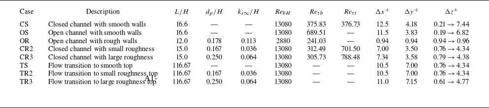


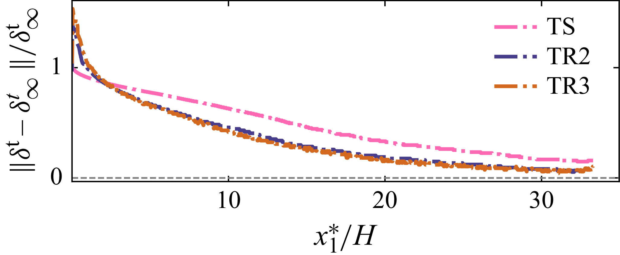


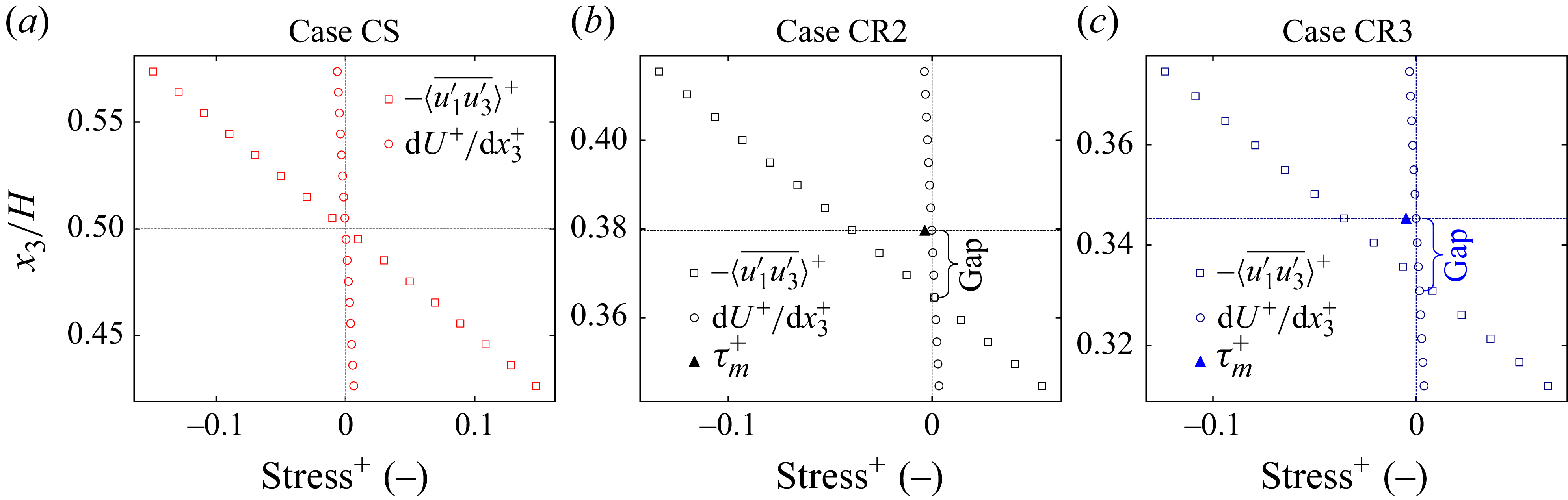


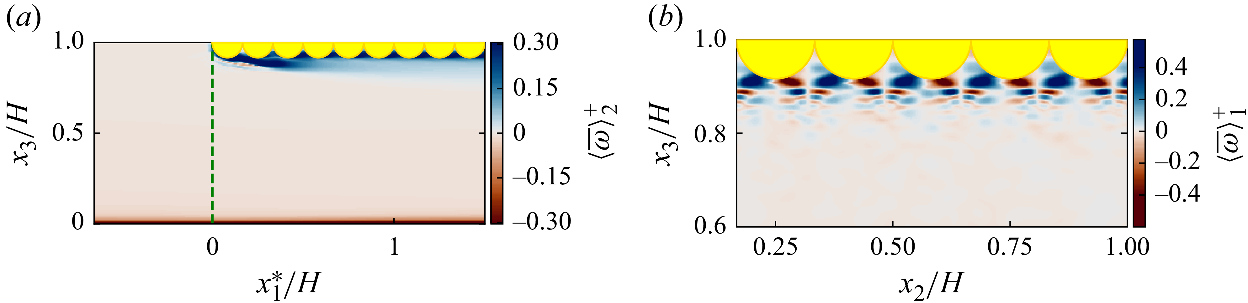


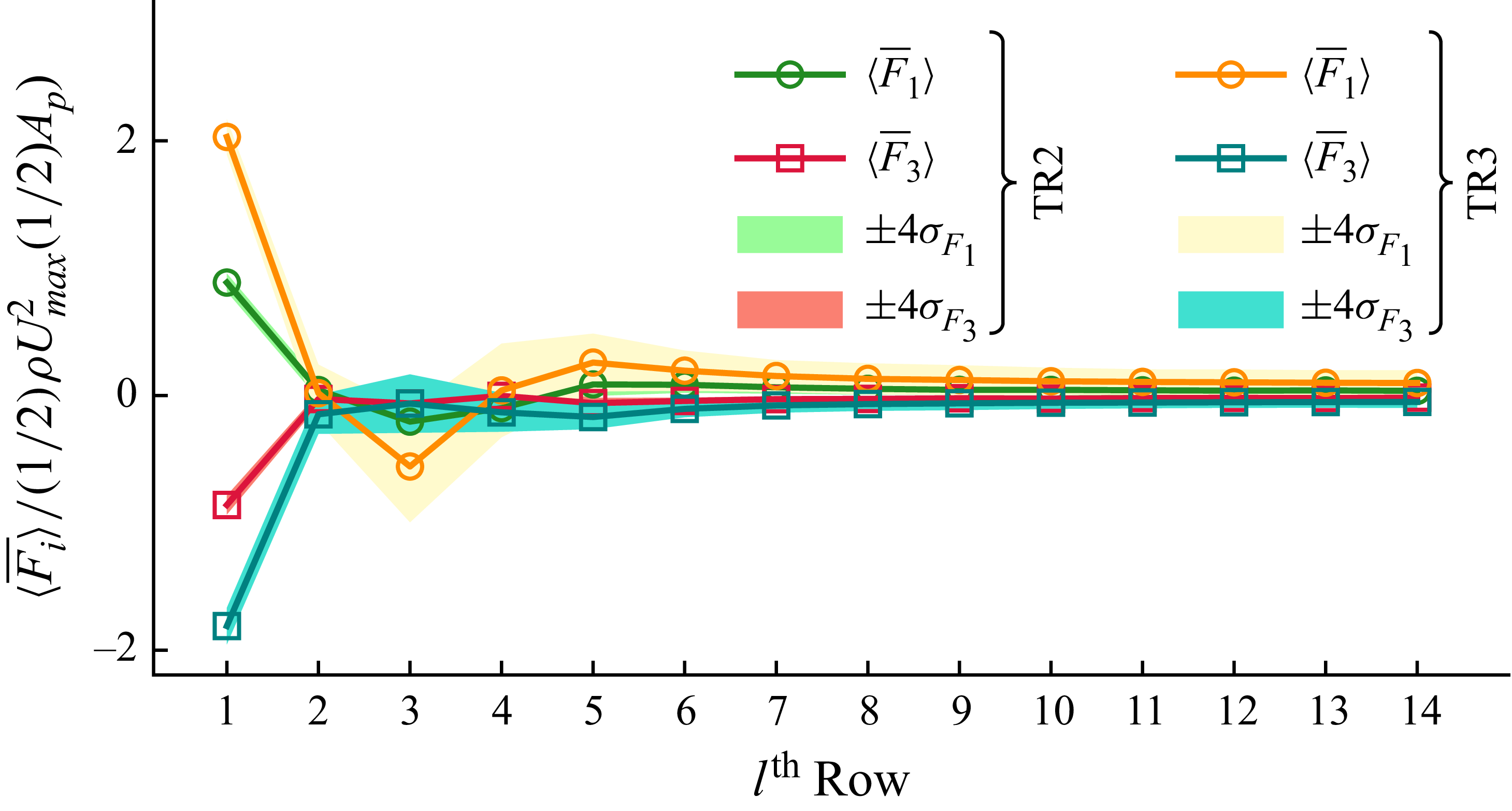


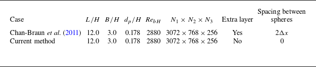


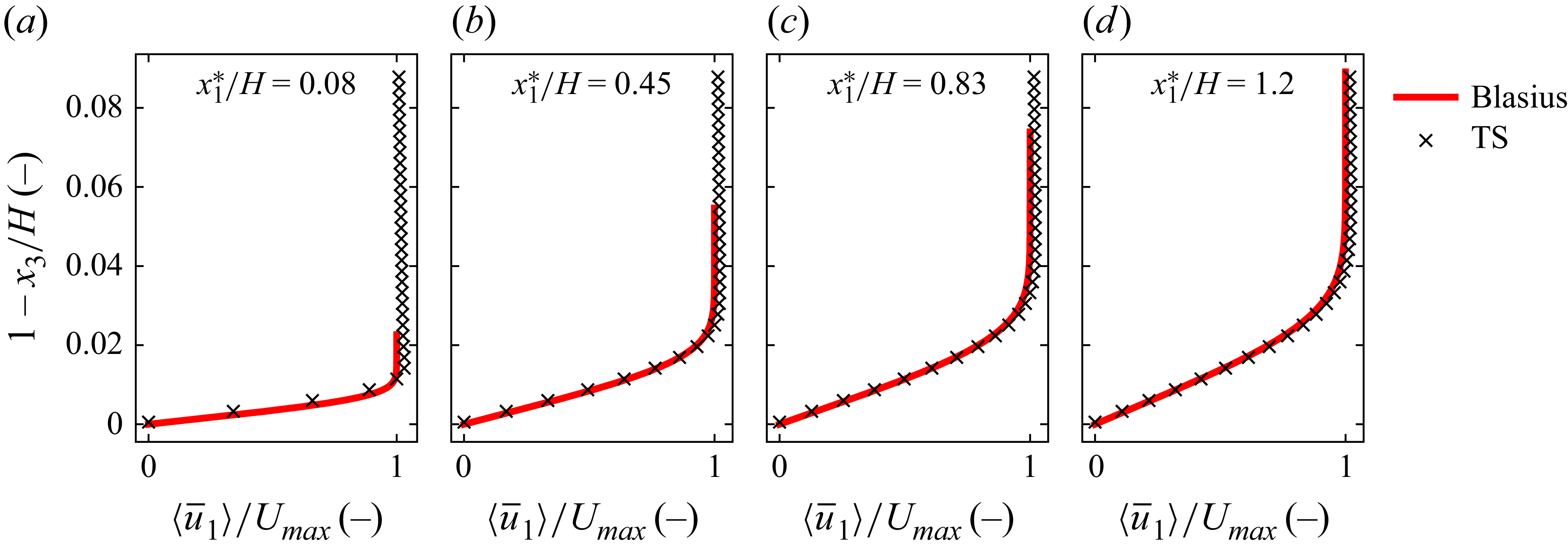


 Open access