


1. Introduction
Taylor dispersion plays a crucial role in the transport and mixing of passive scalars (such as temperature or concentration) in fluid flows, with applications spanning various scientific and engineering disciplines. Originally studied by Taylor (Reference Taylor1953), it describes how a solute in shear flow undergoes enhanced mixing due to the interplay between advection and diffusion. Classical Taylor dispersion theory has been widely utilised, as it enables dimensional reduction by approximating the governing equations with fewer independent variables (Young & Jones Reference Young and Jones1991; Ding Reference Ding2023; Teng, Rallabandi & Ault Reference Teng, Rallabandi and Ault2023; David et al. Reference David, Hester, Xu and Aurnou2024; Guan & Chen Reference Guan and Chen2024). However, since Taylor dispersion is an asymptotic approximation valid at long times, a fundamental question arises: At what time scale does this approximation become valid?
To address this question, it is useful to examine the evolution of the scalar field in a straight channel with uniform cross-section, from its initial introduction into the flow to its eventual homogenisation. This process can be characterised by three distinct time scales: dispersion, longitudinal normality and transverse uniformity, which we outline below.
In the early stage after the solute is injected into the channel, it is primarily advected along streamlines and undergoes stretching. During this stage, advection dominates while diffusion begins to play a role, leading to a complex evolution of the scalar field Taghizadeh, Valdés-Parada & Wood (Reference Taghizadeh, Valdés-Parada and Wood2020), Camassa et al. (Reference Camassa, McLaughlin and Viotti2010b ). The first significant time scale arises when the variance of the solute concentration begins to grow linearly in time, marking the onset of Taylor dispersion Aris (Reference Aris1956), Camassa et al. (Reference Camassa, Lin and McLaughlin2010a ). This signals that diffusion has started to act in concert with the background flow to redistribute the solute along the channel. At this stage, the rate of variance growth exceeds that of pure molecular diffusion due to the coupling between shear-induced advection and transverse diffusion. One might expect that the scalar field could already be described by a diffusion equation, since the solution of a diffusion equation is a Gaussian function with linearly increasing variance. However, at this stage, transverse variations in the scalar field persist, and the cross-sectionally averaged scalar field may still deviate from a Gaussian profile, exhibiting skewness that depends on the channel geometry and shear flow characteristics Aminian et al. (Reference Aminian, Bernardi, Camassa, Harris and McLaughlin2016).
As molecular diffusion continues, the cross-sectionally averaged scalar field approaches a Gaussian distribution, marking the second time scale. Once this stage is reached, the evolution of the cross-sectionally averaged scalar field can be effectively described by a one-dimensional diffusion equation with an enhanced diffusivity Chatwin (Reference Chatwin1970). We refer to this governing equation as the effective equation and to the enhanced diffusion coefficient as the effective diffusivity. However, even at this stage, the solute concentration may still exhibit non-uniformity across the channel cross-section.
The third and final time scale corresponds to the attainment of transverse uniformity across the channel cross-section. At this point, diffusion has sufficiently spread the solute so that the concentration becomes nearly uniform across the cross-section. Wu & Chen (Reference Wu and Chen2014) demonstrated that this time scale can be up to ten times larger than that for longitudinal normality, highlighting the extended duration required for complete transverse homogenisation. At this stage, the whole scalar field can be well approximated by a one-dimensional effective equation.
How do these time scales depend on physical parameters? The enhanced mixing in Taylor dispersion arises from the diffusion of concentration variations across the channel’s cross-section. The time scale for this enhanced mixing is related to the rate at which these variations decay into a uniform concentration through diffusion. Dimensional analysis shows that the diffusion time scale is $L^2/\kappa$
, where
$L^2/\kappa$
, where $L$
is the characteristic length scale of the channel cross-section and
$L$
is the characteristic length scale of the channel cross-section and $\kappa$
is the molecular diffusivity. Interestingly, many studies of Taylor dispersion in a straight channel with flat boundaries show that the variance starts to increase linearly at an earlier time, approximately
$\kappa$
is the molecular diffusivity. Interestingly, many studies of Taylor dispersion in a straight channel with flat boundaries show that the variance starts to increase linearly at an earlier time, approximately $0.1L^2/\kappa$
, for steady shear flows in various geometries, such as parallel plate channels Camassa et al. (Reference Camassa, Lin and McLaughlin2010a
), circular pipes Barton (Reference Barton1983) and even time-dependent flows Vedel & Bruus (Reference Vedel and Bruus2012), Vedel, Hovad & Bruus (Reference Vedel, Hovad and Bruus2014). The variance evolution can be computed exactly using the method of moments, first proposed by Aris (Reference Aris1956). These calculations refine the dispersion time scale to
$0.1L^2/\kappa$
, for steady shear flows in various geometries, such as parallel plate channels Camassa et al. (Reference Camassa, Lin and McLaughlin2010a
), circular pipes Barton (Reference Barton1983) and even time-dependent flows Vedel & Bruus (Reference Vedel and Bruus2012), Vedel, Hovad & Bruus (Reference Vedel, Hovad and Bruus2014). The variance evolution can be computed exactly using the method of moments, first proposed by Aris (Reference Aris1956). These calculations refine the dispersion time scale to $L^2/(\kappa \lambda )$
, where
$L^2/(\kappa \lambda )$
, where $\lambda$
is the smallest non-zero eigenvalue of the Laplacian on the cross-section domain. For a parallel plate channel,
$\lambda$
is the smallest non-zero eigenvalue of the Laplacian on the cross-section domain. For a parallel plate channel, $L$
is the gap width,
$L$
is the gap width, $\lambda = \pi ^2$
and
$\lambda = \pi ^2$
and $1/\lambda \approx 0.1$
. For a circular pipe with radial symmetry,
$1/\lambda \approx 0.1$
. For a circular pipe with radial symmetry, $L$
is the radius,
$L$
is the radius, $\lambda = 14.682$
(the square of the roots of
$\lambda = 14.682$
(the square of the roots of $J_1(x)$
, the Bessel function of the first kind of order one), yielding
$J_1(x)$
, the Bessel function of the first kind of order one), yielding $1/\lambda \approx 0.0681$
.
$1/\lambda \approx 0.0681$
.
In addition to studies focusing on the variance, others investigate the approximation of the entire scalar field. Mercer & Roberts (Reference Mercer and Roberts1990), Watt & Roberts (Reference Watt and Roberts1995) demonstrated that the scalar field converges exponentially to the centre manifold of the system, and the rate of this convergence is governed by the Laplacian eigenvalue. This implies that the time scale for achieving longitudinal normality is also closely related to $L^2/(\kappa \lambda )$
. Stokes & Barton (Reference Stokes and Barton1990), Phillips & Kaye (Reference Phillips and Kaye1996) applied a Laplace transform in time and a Fourier transform in the longitudinal direction to derive an integral representation of the concentration field, enabling accurate asymptotic expansions at both short and long times. Using a representation that combines the Fourier transform with eigenfunction expansion, Ding & McLaughlin (Reference Ding and McLaughlin2022b
) derived an effective equation and effective diffusivity for a family of stochastic shear flows, demonstrating that the time scale is governed by the Laplacian eigenvalues associated with the random scalar field.
$L^2/(\kappa \lambda )$
. Stokes & Barton (Reference Stokes and Barton1990), Phillips & Kaye (Reference Phillips and Kaye1996) applied a Laplace transform in time and a Fourier transform in the longitudinal direction to derive an integral representation of the concentration field, enabling accurate asymptotic expansions at both short and long times. Using a representation that combines the Fourier transform with eigenfunction expansion, Ding & McLaughlin (Reference Ding and McLaughlin2022b
) derived an effective equation and effective diffusivity for a family of stochastic shear flows, demonstrating that the time scale is governed by the Laplacian eigenvalues associated with the random scalar field.
While the theory for channels with flat walls is well developed, real-world systems often involve more complex geometries, such as channels with periodically varying cross-sections (Roggeveen, Stone & Kurzthaler Reference Roggeveen, Stone and Kurzthaler2023). These geometries are crucial in applications like passive microfluidic mixers and flow through porous media. Micro passive mixers enable rapid homogenisation, essential for chemical and biological processes at the microscale. Specially designed channel boundaries can enhance mixing by inducing chaotic advection (Liu et al. Reference Liu, Stremler, Sharp, Olsen, Santiago, Adrian, Aref and Beebe2000; Stroock et al. Reference Stroock, Dertinger, Ajdari, Mezic, Stone and Whitesides2002; Stone, Stroock & Ajdari Reference Stone, Stroock and Ajdari2004; Oevreeide et al. Reference Oevreeide, Zoellner, Mielnik and Stokke2020), leading to faster homogenisation compared with shear-driven mixing in straight channels. In addition, a sinusoidally varying channel radius serves as an idealised model for flow through porous media, where constrictions and expansions mimic pore throats and pore bodies (Richmond et al. Reference Richmond, Perkins, Scheibe, Lambert and Wood2013; Liu et al. Reference Liu, Xiao, Aquino, Dentz and Wang2024). In both cases, generalised Taylor dispersion theory provides a framework for estimating the longitudinal dispersion coefficient and approximating the scalar field (Brenner Reference Brenner1980; Hoagland & Prud’Homme Reference Hoagland and Prud’Homme1985; Amaral Souto & Moyne Reference Amaral Souto and Moyne1997; DeGroot & Straatman Reference DeGroot and Straatman2011, Haugerud, Linga & Flekkøy Reference Haugerud, Linga and Flekkøy2022). Thus, determining the characteristic time for the validity of Taylor dispersion theory is of fundamental importance.
Several numerical studies have attempted to estimate the characteristic time scale. For instance, Bouquain et al. (Reference Bouquain, Méheust, Bolster and Davy2012) investigated sinusoidally varying channels and estimated the characteristic time by fitting the numerically computed time evolution of the normalised dispersion coefficient to an exponential relaxation function. Haugerud et al. (Reference Haugerud, Linga and Flekkøy2022) investigated channels with periodic square boundary roughness. Non-flat boundaries can induce circulation regions that trap particles and affect the dispersion process. Haugerud et al. (Reference Haugerud, Linga and Flekkøy2022) showed that particle residence times in these circulation regions are directly related to the characteristic mixing time. However, these approaches rely on simulating the scalar field over the entire domain, which is computationally expensive, particularly in geometries with complex boundaries. Despite valuable insights, a rigorous and systematic theoretical framework for estimating mixing times in such domains remains an open challenge.
As mentioned earlier, in the case of scalar transport in a channel with flat boundaries, the approach combining the Fourier transform in the longitudinal direction with eigenfunction expansion has been successful in analysing characteristic times. However, two main challenges arise when generalising this method to a channel with periodically varying cross-sections. First, the Fourier transform in the axial direction is no longer applicable due to the complex geometry. Second, while the flow may be periodic and solvable within a unit cell, the scalar field itself is not periodic. As a result, the eigenfunctions of the advection--diffusion operator must be defined over the entire domain rather than a single cell. Since exact solutions to this eigenvalue problem are typically unavailable, numerical methods are required. However, solving on an infinite domain poses computational challenges, making this approach impractical.
To overcome the challenges of solving the advection--diffusion equation in a periodic channel, we introduce a Floquet–Bloch-type eigenfunction representation that separates the non-periodic and periodic components of the scalar field. This reduces the eigenvalue problem from the full domain to a simpler one defined on a single unit cell. These eigenfunctions form a complete basis for square-integrable functions, enabling an integral representation of the scalar field. This representation highlights the mode governing the system’s slow dynamics, leading to a reduced model whose difference from the full system decays exponentially in time. This reduced model allows us to rigorously determine the time scale over which Taylor dispersion theory remains valid. By applying the method of steepest descent to the integral representation of the slow manifold, we derive the long-time asymptotic expansion of the scalar field. This approach reveals the structure of the advection--diffusion solution in a periodic channel and clarifies the relationships among key dispersion time scales: longitudinal normality, transverse uniformity and effective dispersion. The dominant time scale depends solely on the flow and domain geometries and can be computed from the solution within a single unit cell. Together, these results offer a rigorous and systematic framework for estimating mixing time scales in complex geometries.
This paper is organised as follows. In § 2 we first formulate the governing equations for the scalar field and fluid flow and outline the non-dimensionalisation process. We then define the eigenvalue problem and present the eigenfunction expansion of the scalar field. Based on this, we identify the system’s slow manifold and derive the long-time asymptotic expansion of the scalar field. Next, we discuss the relationship between different time scales in the Taylor dispersion problem. Section 3 examines the characteristic time for the scalar field to converge to the slow manifold through several examples. In § 4 we briefly discuss extending the proposed method to porous media. In § 5 we summarise our findings and explore potential directions for future research. Appendix A provides the perturbation calculations for the small-wavenumber expansion of the eigenfunctions, while Appendix B details the numerical methods used in this study.
2. Governing equation and asymptotic analysis
We consider a straight channel domain of length $L$
with a periodically varying cross-section, defined as
$L$
with a periodically varying cross-section, defined as
 \begin{equation} \begin{aligned} \varOmega (L) = \left \{ (x, \boldsymbol{y}) \,|\, -\frac {L}{2} \leqslant x \leqslant \frac {L}{2}, \, \boldsymbol{y} \in \varOmega _{c}(x) \right \}\!, \end{aligned} \end{equation}
where the $x$
direction is the longitudinal axis of the channel and
$x$
direction is the longitudinal axis of the channel and $\varOmega _{c}(x) \subset \mathbb{R}^{d}$
denotes the cross-section of the channel, which depends on
$\varOmega _{c}(x) \subset \mathbb{R}^{d}$
denotes the cross-section of the channel, which depends on $x$
. We assume that
$x$
. We assume that $\varOmega _{c}(x)$
is periodic in
$\varOmega _{c}(x)$
is periodic in $x$
with a period
$x$
with a period $L_{p}$
. We often focus on the case of an infinitely long channel, denoting it as
$L_{p}$
. We often focus on the case of an infinitely long channel, denoting it as $\varOmega = \varOmega (\infty )$
for simplicity. The volume of the channel is represented as
$\varOmega = \varOmega (\infty )$
for simplicity. The volume of the channel is represented as $|\varOmega (L)|$
, while the average cross-sectional area is given by
$|\varOmega (L)|$
, while the average cross-sectional area is given by $|\varOmega _{c}| = {|\varOmega (L_{p})|}/{L_{p}}$
. The simplest case is a domain bounded by two wavy walls:
$|\varOmega _{c}| = {|\varOmega (L_{p})|}/{L_{p}}$
. The simplest case is a domain bounded by two wavy walls: $\varOmega = \left \{ (x, y) \,|\, x \in \mathbb{R}, \, h_{1}(x) \leqslant y \leqslant h_{2}(x) \right \}$
, where
$\varOmega = \left \{ (x, y) \,|\, x \in \mathbb{R}, \, h_{1}(x) \leqslant y \leqslant h_{2}(x) \right \}$
, where $h_{1}(x)$
and
$h_{1}(x)$
and $h_{2}(x)$
share the same period
$h_{2}(x)$
share the same period $L_{p}$
. In this scenario, the average cross-sectional area is calculated as
$L_{p}$
. In this scenario, the average cross-sectional area is calculated as $|\varOmega _{c}| =( {1}/{L_{p}} )\int _{0}^{L_{p}} (h_{2}(x) - h_{1}(x)) \, \mathrm{d} x$
. Beyond this type of domain, practical examples include axisymmetric channels (Chang & Santiago Reference Chang and Santiago2023) and curved microfluidic channels (Liu et al. Reference Liu, Stremler, Sharp, Olsen, Santiago, Adrian, Aref and Beebe2000; Stroock et al. Reference Stroock, Dertinger, Ajdari, Mezic, Stone and Whitesides2002).
$|\varOmega _{c}| =( {1}/{L_{p}} )\int _{0}^{L_{p}} (h_{2}(x) - h_{1}(x)) \, \mathrm{d} x$
. Beyond this type of domain, practical examples include axisymmetric channels (Chang & Santiago Reference Chang and Santiago2023) and curved microfluidic channels (Liu et al. Reference Liu, Stremler, Sharp, Olsen, Santiago, Adrian, Aref and Beebe2000; Stroock et al. Reference Stroock, Dertinger, Ajdari, Mezic, Stone and Whitesides2002).
The passive scalar is governed by the advection--diffusion equation with no-flux boundary conditions, which takes the form
 \begin{equation} \begin{aligned} &\partial _{t} c + \boldsymbol{u} \boldsymbol{\cdot }\boldsymbol{\nabla }c = \boldsymbol{\nabla }\boldsymbol{\cdot }(\kappa \boldsymbol{\nabla }c) , \quad c (x, \boldsymbol{y}, 0) = c_{I} (x, \boldsymbol{y}), \quad \left . \boldsymbol{n} \boldsymbol{\cdot }\boldsymbol{\nabla }c \right |_{w\textit{all}} = 0, \end{aligned} \end{equation}
where $\kappa$
is the diffusivity and
$\kappa$
is the diffusivity and $c_{I}$
is the initial condition, which is assumed to be non-negative. The vector
$c_{I}$
is the initial condition, which is assumed to be non-negative. The vector $\boldsymbol{n} = (n_{x}, n_{1}, \ldots , n_{d})$
denotes the outward normal to the boundary and
$\boldsymbol{n} = (n_{x}, n_{1}, \ldots , n_{d})$
denotes the outward normal to the boundary and $\boldsymbol{u}$
is the velocity field. The theory developed in this paper can be readily generalised to the case where
$\boldsymbol{u}$
is the velocity field. The theory developed in this paper can be readily generalised to the case where $\kappa$
is a spatially periodic function, i.e.
$\kappa$
is a spatially periodic function, i.e. $\kappa = \kappa (x, \boldsymbol{y})$
, but for simplicity, we assume it to be constant throughout this work. To ensure mass conservation, we assume that the velocity field is incompressible and satisfies the no-flux boundary condition. Additionally, we consider flows that are periodic in the longitudinal direction of the channel, with a fundamental period
$\kappa = \kappa (x, \boldsymbol{y})$
, but for simplicity, we assume it to be constant throughout this work. To ensure mass conservation, we assume that the velocity field is incompressible and satisfies the no-flux boundary condition. Additionally, we consider flows that are periodic in the longitudinal direction of the channel, with a fundamental period $L_{p}$
. While the theoretical results developed here apply to any velocity field satisfying these assumptions, the simulations presented use velocity fields governed by the Navier–Stokes equations. For a homogeneous fluid, the velocity field
$L_{p}$
. While the theoretical results developed here apply to any velocity field satisfying these assumptions, the simulations presented use velocity fields governed by the Navier–Stokes equations. For a homogeneous fluid, the velocity field $\boldsymbol{u} = (u, \boldsymbol{v})$
satisfies the Navier–Stokes equations:
$\boldsymbol{u} = (u, \boldsymbol{v})$
satisfies the Navier–Stokes equations:
 \begin{equation} \begin{aligned} &\partial _{t} u + u \partial _{x} u + \boldsymbol{v} \boldsymbol{\cdot }\boldsymbol{\nabla} _{\boldsymbol{y}} u = -\frac {1}{\rho _{0}} \partial _{x} p + \nu \big ( \partial _{x}^{2} u + \Delta _{\boldsymbol{y}} u \big )+f_{x}, \\&\partial _{t} v_{i} + u \partial _{x} v_{i} + \boldsymbol{v} \boldsymbol{\cdot }\boldsymbol{\nabla} _{\boldsymbol{y}} v_{i} = -\frac {1}{\rho _{0}} \partial _{y_{i}} p + \nu \big ( \partial _{x}^{2} v_{i} + \Delta _{\boldsymbol{y}} v_{i} \big )+f_{y,i}, \quad i = 1, \ldots , d, \\&\partial _{x} u + \boldsymbol{\nabla} _{\boldsymbol{y}} \boldsymbol{\cdot }\boldsymbol{v} = 0, \quad \left . \boldsymbol{u} \right |_{w\textit{all}} = 0. \end{aligned} \end{equation}
Here $u$
is the fluid velocity in the longitudinal
$u$
is the fluid velocity in the longitudinal $x$
direction,
$x$
direction, $v_i$
is the fluid velocity aligned with the
$v_i$
is the fluid velocity aligned with the $y_i$
directions,
$y_i$
directions, $\boldsymbol{v} = (v_{1}, \ldots , v_{d})$
,
$\boldsymbol{v} = (v_{1}, \ldots , v_{d})$
, $p$
is the pressure,
$p$
is the pressure, $\rho _{0}$
is the fluid density and
$\rho _{0}$
is the fluid density and $\nu$
is the fluid kinematic viscosity. The subscript
$\nu$
is the fluid kinematic viscosity. The subscript $\boldsymbol{y}$
denotes quantities related to the coordinates in the cross-section, where
$\boldsymbol{y}$
denotes quantities related to the coordinates in the cross-section, where $\boldsymbol{n}_{\boldsymbol{y}} = (n_{1}, \ldots , n_{d})$
,
$\boldsymbol{n}_{\boldsymbol{y}} = (n_{1}, \ldots , n_{d})$
, $\boldsymbol{\nabla} _{\boldsymbol{y}} = (\partial _{y_{1}}, \ldots , \partial _{y_{d}})$
and
$\boldsymbol{\nabla} _{\boldsymbol{y}} = (\partial _{y_{1}}, \ldots , \partial _{y_{d}})$
and $\Delta _{\boldsymbol{y}} = \sum _{i=1}^{d} \partial _{y_{i}}^{2}$
. The forcing terms
$\Delta _{\boldsymbol{y}} = \sum _{i=1}^{d} \partial _{y_{i}}^{2}$
. The forcing terms $f_{x}$
and
$f_{x}$
and $f_{y_{i}}$
represent external forces. In pressure-driven flow,
$f_{y_{i}}$
represent external forces. In pressure-driven flow, $f_{x}$
is a constant while
$f_{x}$
is a constant while $f_{y_{i}} = 0$
. If the domain boundary is periodic, it induces periodicity in the flow, as illustrated in figure 1, satisfying our assumption about the velocity field structure. While a transient region exists near the inlet, the flow converges exponentially to the periodic state (Feppon Reference Feppon2025). Therefore, our analysis focuses on the fully developed periodic flow.
$f_{y_{i}} = 0$
. If the domain boundary is periodic, it induces periodicity in the flow, as illustrated in figure 1, satisfying our assumption about the velocity field structure. While a transient region exists near the inlet, the flow converges exponentially to the periodic state (Feppon Reference Feppon2025). Therefore, our analysis focuses on the fully developed periodic flow.
A pressure-driven flow passes from left to right through a channel with periodically varying cross-sections. Two unit cells of the periodic pattern are displayed. The velocity magnitude in the recirculating region is about one-tenth of that in the main flow stream; therefore, the arrow lengths have been scaled to enhance the visibility of the recirculation. The flow field was obtained using FreeFem++ with the algorithm described in Appendix B.

2.1. Non-dimensionalisation
We denote the characteristic length scale of the channel cross-section as $L_{y}$
. We then proceed with the following change of variables for non-dimensionalisation:
$L_{y}$
. We then proceed with the following change of variables for non-dimensionalisation:
 \begin{equation} \begin{aligned} &L_{y} \tilde {x}=x, \quad L_{y} \tilde {\boldsymbol{y}}=\boldsymbol{y},\quad U \tilde {u} =u, \quad U \tilde {\boldsymbol{v}}=\boldsymbol{v}, \quad \frac {\rho _{0}\nu U}{L_{y}} \tilde {p}=p, \quad \frac {L_{y}^{2}}{\kappa }\tilde {t}=t,\quad c_{c}\tilde {c}=c. \end{aligned} \end{equation}
Equation (2.2) becomes
 \begin{equation} \begin{aligned} &\partial _{\tilde {t}} \tilde {c}+\frac {U}{L_{y}}\tilde {\boldsymbol{u}}\boldsymbol{\cdot }\boldsymbol{\nabla }\tilde {c} = \frac {\kappa }{L_{y}^{2}} \Delta \tilde {c}, \quad \left . \frac {1}{L_{y}} \boldsymbol{n} \boldsymbol{\cdot }\boldsymbol{\nabla }\tilde {c} \right |_{w\textit{all}}=0 ,\end{aligned} \end{equation}
and (2.3) becomes
 \begin{equation} \begin{aligned} & \frac {U \kappa }{L_{y}^{2}} \partial _{\tilde {t}}\tilde {u}+ \frac {U^{2}}{L_{y}} \tilde {u} \partial _{\tilde {x}}\tilde {u} + \frac {U^{2}}{L_{y}} \tilde {\boldsymbol{v}} \boldsymbol{\cdot }\partial _{\tilde {\boldsymbol{y}}}\tilde {u}= -\frac {\nu U}{L_{y}^{2}} \partial _{\tilde {x}}\tilde {p} + \nu U \left ( \frac {1}{L_{y}^{2}} \partial _{\tilde {x}}^{2}\tilde {u} + \frac {1}{L_{y}^{2}} \Delta _{\tilde {\boldsymbol{y}}}^{2}\tilde {u} \right )\!,\\ & \frac {U \kappa }{L_{y}^{2}} \partial _{\tilde {t}}\tilde {v}_{i}+ \frac {U^{2}}{L_{y}} \tilde {u} \partial _{\tilde {x}}\tilde {v}_{i} + \frac {U^{2}}{L_{y}} \tilde {\boldsymbol{v}}\boldsymbol{\cdot }\partial _{\tilde {\boldsymbol{y}}}\tilde {v}_{i}= -\frac {\nu U}{L_{y}^{2}} \partial _{\tilde {y}_{i}}\tilde {p} + \nu U \left ( \frac {1}{L_{y}^{2}} \partial _{\tilde {x}}^{2}\tilde {v}_{i} + \frac {1}{L_{y}^{2}} \Delta _{\tilde {\boldsymbol{y}}}^{2}\tilde {v}_{i} \right )\!,\\ &\frac {U}{L_{y}}\partial _{\tilde {x}}\tilde {u}+\frac {U}{L_{y}}\boldsymbol{\nabla} _{\tilde {\boldsymbol{y}}} \boldsymbol{\cdot }\tilde {\boldsymbol{v}}=0. \end{aligned} \end{equation}
Now the velocity field $\tilde {\boldsymbol{u}}$
has the dimensionless fundamental period
$\tilde {\boldsymbol{u}}$
has the dimensionless fundamental period $\tilde {L}_{p} = L_{p} / L_{y}$
. After dropping the tilde, we obtain the equation for the scalar field
$\tilde {L}_{p} = L_{p} / L_{y}$
. After dropping the tilde, we obtain the equation for the scalar field
 \begin{equation} \begin{aligned} &\partial _{t} c+ {\textit{Pe}} \boldsymbol{u} \boldsymbol{\cdot }\boldsymbol{\nabla }c = \Delta c ,\quad c (x,\boldsymbol{y},0) = c_{I} \left ( x,\boldsymbol{y}\right )\!,\quad \left . \boldsymbol{n}\boldsymbol{\cdot }\boldsymbol{\nabla }c \right |_{w\textit{all}}=0, \end{aligned} \end{equation}
and the equation for the velocity field
 \begin{equation} \begin{aligned} &\frac {1}{{Sc}}\partial _{t}u+ {\textit{Re}}\left ( u \partial _{x}u + \boldsymbol{v} \boldsymbol{\cdot }\boldsymbol{\nabla} _{\boldsymbol{y}}u \right )= -\partial _{x}p + \big ( \partial _{x}^{2}u + \Delta _{\boldsymbol{y}}u \big ),\\&\frac {1}{{Sc}}\partial _{t}v_{i}+ {\textit{Re}} \left ( u \partial _{x}v_{i} + \boldsymbol{v}\boldsymbol{\cdot }\boldsymbol{\nabla} _{\boldsymbol{y}}v_{i} \right )= - \partial _{y_{i}}p + \big ( \partial _{x}^{2}v_{i} + \Delta _{\boldsymbol{y}}v_{i} \big ),\\&\partial _{x}u+\boldsymbol{\nabla} _{\boldsymbol{y}} \boldsymbol{\cdot }\boldsymbol{v}=0,\quad \left . \boldsymbol{u} \right |_{w\textit{all}}=0, \end{aligned} \end{equation}
where we have defined the Pélect number ${\textit{Pe}}={L_{y}U}/{\kappa }$
, the Reynolds number
${\textit{Pe}}={L_{y}U}/{\kappa }$
, the Reynolds number ${\textit{Re}}={ L_{y}U}/{\nu }$
and the Schmidt number
${\textit{Re}}={ L_{y}U}/{\nu }$
and the Schmidt number ${Sc}={\nu }/{ \kappa }$
. Unless otherwise noted, all quantities in the subsequent sections, including
${Sc}={\nu }/{ \kappa }$
. Unless otherwise noted, all quantities in the subsequent sections, including $\tilde {L}_{p}$
, are taken to be dimensionless, and for simplicity, we drop the tilde.
$\tilde {L}_{p}$
, are taken to be dimensionless, and for simplicity, we drop the tilde.
2.2. Variance and effective longitudinal diffusivity
Since the solution of the advection–diffusion equation in a channel domain converges to a Gaussian distribution at long times, the variance serves as a key quantity for characterising the solution. In this section we present its definition.
As the following discussion involves complex-valued functions, we define the inner product as
 \begin{equation} \left \langle f, g \right \rangle = \frac {1}{|\varOmega (L_p)|} \int \limits _{\varOmega } f(x, \boldsymbol{y}) g^{*}(x, \boldsymbol{y}) \,\mathrm{d}x \,\mathrm{d}\boldsymbol{y}, \end{equation}
where the asterisk denotes the complex conjugate. For simplicity, we use the notation $\left \langle u \right \rangle$
as a shorthand for
$\left \langle u \right \rangle$
as a shorthand for $\left \langle u, 1 \right \rangle$
.
$\left \langle u, 1 \right \rangle$
.
Since the solution approaches a Gaussian function at long times, its variance is given by
 \begin{equation} \begin{aligned} \text{Var}_{c}(t) &= \frac {\left \langle (x-\left \langle xc \right \rangle )^{2}c \right \rangle }{\left \langle c \right \rangle }=\frac {\left \langle x^{2}c \right \rangle - \left \langle xc \right \rangle ^{2}}{\left \langle c \right \rangle }. \end{aligned} \end{equation}
Then the effective longitudinal diffusivity is defined as
 \begin{equation} \kappa _{\textit{eff}} = \lim \limits _{t\rightarrow \infty } \frac {\text{Var}_{c}(t)}{2t} = \lim \limits _{t\rightarrow \infty } \frac {1}{2} \partial _{t} \text{Var}_{c}(t). \end{equation}
In some studies on time-dependent flows, the term $({1}/{2}) \partial _{t} \text{Var}(t)$
is directly defined as the effective diffusivity, as seen in Vedel & Bruus (Reference Vedel and Bruus2012), Vedel et al. (Reference Vedel, Hovad and Bruus2014), Ding & McLaughlin (Reference Ding and McLaughlin2023).
$({1}/{2}) \partial _{t} \text{Var}(t)$
is directly defined as the effective diffusivity, as seen in Vedel & Bruus (Reference Vedel and Bruus2012), Vedel et al. (Reference Vedel, Hovad and Bruus2014), Ding & McLaughlin (Reference Ding and McLaughlin2023).
2.3. Eigenfunction expansion
Since the advection--diffusion equation (2.2) is linear, the eigenfunction expansion of the scalar field is a convenient tool for analysing scalar dynamics. The eigenvalue $\lambda$
and eigenfunction
$\lambda$
and eigenfunction $\phi$
satisfy the following equation:
$\phi$
satisfy the following equation:
 \begin{equation} \begin{aligned} &\lambda \phi = \mathcal{L} \phi = {\textit{Pe}} \left ( u \partial _{x} \phi + \boldsymbol{v} \boldsymbol{\cdot }\boldsymbol{\nabla} _{\boldsymbol{y}} \phi \right ) - \partial _{x}^{2} \phi - \Delta _{\boldsymbol{y}} \phi , \quad \left . n_{x} \partial _{x} \phi + \partial _{\boldsymbol{n}_{y}} \phi \right |_{w\textit{all}} = 0. \end{aligned} \end{equation}
It forms a basis for square-integrable functions defined on the infinite channel domain that satisfy the no-flux boundary condition $\left . n_{x} \partial _{x} \phi + \partial _{\boldsymbol{n}_{y}} \phi \right |_{w\textit{all}} = 0$
.
$\left . n_{x} \partial _{x} \phi + \partial _{\boldsymbol{n}_{y}} \phi \right |_{w\textit{all}} = 0$
.
There are three properties of eigenvalues and eigenfunctions that will be used later. First, given that the velocity field is real, $\lambda ^{*}$
is also an eigenvalue and
$\lambda ^{*}$
is also an eigenvalue and $\phi ^{*}$
is the associated eigenfunction. Second, the real part of the eigenvalue is non-negative (see the proof in Appendix A.1). Third,
$\phi ^{*}$
is the associated eigenfunction. Second, the real part of the eigenvalue is non-negative (see the proof in Appendix A.1). Third, $\lambda = 0$
is the smallest eigenvalue and
$\lambda = 0$
is the smallest eigenvalue and $\phi = 1$
is the associated eigenfunction.
$\phi = 1$
is the associated eigenfunction.
Since the advection operator is a skew-adjoint operator, $\mathcal{L}$
is not a self-adjoint operator when the velocity field is non-zero. Hence, we introduce
$\mathcal{L}$
is not a self-adjoint operator when the velocity field is non-zero. Hence, we introduce $\lambda ^{*}$
and
$\lambda ^{*}$
and $\varphi (x, \boldsymbol{y})$
, which are the eigenvalues and eigenfunctions of the adjoint eigenvalue problem given by
$\varphi (x, \boldsymbol{y})$
, which are the eigenvalues and eigenfunctions of the adjoint eigenvalue problem given by
 \begin{equation} \begin{aligned} &\lambda ^{*} \varphi = \mathcal{L}^{*} \varphi = -{\textit{Pe}} \left ( u \partial _{x} \varphi + \boldsymbol{v} \boldsymbol{\cdot }\boldsymbol{\nabla} _{\boldsymbol{y}} \varphi \right ) - \partial _{x}^{2} \varphi - \Delta _{\boldsymbol{y}} \varphi , \quad \left . n_{x} \partial _{x} \varphi + \partial _{\boldsymbol{n}_{y}} \varphi \right |_{w\textit{all}} = 0. \end{aligned} \end{equation}
In the adjoint eigenvalue problem, ${\textit{Pe}}$
is replaced with
${\textit{Pe}}$
is replaced with $-{\textit{Pe}}$
, effectively reversing the flow direction.
$-{\textit{Pe}}$
, effectively reversing the flow direction.
Next, we choose $\phi _{n}$
and
$\phi _{n}$
and $\varphi _{n}$
such that the sets
$\varphi _{n}$
such that the sets $\left \{ \phi _{n} \right \}_{n=0}^{\infty }$
and
$\left \{ \phi _{n} \right \}_{n=0}^{\infty }$
and $\left \{ \varphi _{n} \right \}_{n=0}^{\infty }$
form a biorthogonal system, i.e.
$\left \{ \varphi _{n} \right \}_{n=0}^{\infty }$
form a biorthogonal system, i.e. $\left \langle \phi _{n}, \varphi _{m} \right \rangle = \delta _{n,m}$
, where
$\left \langle \phi _{n}, \varphi _{m} \right \rangle = \delta _{n,m}$
, where $\delta _{n,m}$
is the Kronecker delta. The solution of the advection--diffusion equation
$\delta _{n,m}$
is the Kronecker delta. The solution of the advection--diffusion equation $\partial _{t} c = \mathcal{L} c$
can be formally represented as
$\partial _{t} c = \mathcal{L} c$
can be formally represented as
 \begin{align} c(x, \boldsymbol{y}, t) = \sum _{n} \left \langle c_{I}(x, \boldsymbol{y}), \varphi _{n}(x, \boldsymbol{y}) \right \rangle \phi _{n}(x, \boldsymbol{y}) \text{e}^{-\lambda _{n} t}. \end{align}
The exact solution to this eigenvalue problem is typically unavailable, necessitating the use of numerical methods. However, the infinite domain presents challenges for numerical computations. One significant simplification of the problem is to consider the eigenfunctions in the form
 \begin{equation} \begin{aligned} &\phi (x, \boldsymbol{y}, k) =\frac {1}{\sqrt {2\pi }} e^{\mathrm{i} k x} \hat {\phi }(x, \boldsymbol{y}, k), \quad \varphi (x, \boldsymbol{y}, k) = \frac {1}{\sqrt {2\pi }} e^{\mathrm{i} k x} \hat {\varphi }(x, \boldsymbol{y}, k), \end{aligned} \end{equation}
where $\hat {\phi }(x, \boldsymbol{y}, k)$
solves the equation
$\hat {\phi }(x, \boldsymbol{y}, k)$
solves the equation
 \begin{align} &\lambda \hat {\phi } = \kern2pt \hat{\kern-2pt \mathcal{L}}(k) \hat {\phi } = {\textit{Pe}} \big ( \mathrm{i} k u \hat {\phi } + u \partial _{x} \hat {\phi } + \boldsymbol{v} \boldsymbol{\cdot }\boldsymbol{\nabla} _{\boldsymbol{y}} \hat {\phi } \big ) - \big ( \partial _{x}^{2} \hat {\phi } + 2\mathrm{i} k \partial _{x} \hat {\phi } + (\mathrm{i} k)^{2} \hat {\phi } + \Delta _{\boldsymbol{y}} \hat {\phi } \big ),\nonumber\\& \left . n_{x} \mathrm{i} k \hat {\phi } + n_{x} \partial _{x} \hat {\phi } + \partial _{\boldsymbol{n}_{y}} \hat {\phi } \right |_{w\textit{all}} = 0, \quad \hat {\phi }(x, \boldsymbol{y}, k)=\hat {\phi }(x+L_{p}, \boldsymbol{y}, k), \end{align}
and $\hat {\varphi }(x, \boldsymbol{y}, k)$
solves the adjoint equation
$\hat {\varphi }(x, \boldsymbol{y}, k)$
solves the adjoint equation
 \begin{align} &\lambda ^{*} \hat {\varphi } = \kern2pt \hat{\kern-2pt \mathcal{L}^{*}}(k) \hat {\varphi } = -{\textit{Pe}} \left ( \mathrm{i} k u \hat {\varphi } + u \partial _{x} \hat {\varphi } + \boldsymbol{v} \boldsymbol{\cdot }\boldsymbol{\nabla} _{\boldsymbol{y}} \hat {\varphi } \right ) - \big ( \partial _{x}^{2} \hat {\varphi } + 2\mathrm{i} k \partial _{x} \hat {\varphi } + (\mathrm{i} k)^{2} \hat {\varphi } + \Delta _{\boldsymbol{y}} \hat {\varphi } \big ),\nonumber \\& \left . n_{x} \mathrm{i} k \hat {\varphi } + n_{x} \partial _{x} \hat {\varphi } + \partial _{\boldsymbol{n}_{y}} \hat {\varphi } \right |_{w\textit{all}} = 0, \quad \hat {\varphi }(x, \boldsymbol{y}, k)=\hat {\varphi }(x+L_{p}, \boldsymbol{y}, k). \end{align}
A key observation is that $\hat {\phi }$
and
$\hat {\phi }$
and $\hat {\varphi }$
have a fundamental period of
$\hat {\varphi }$
have a fundamental period of $L_p$
, whereas the functions
$L_p$
, whereas the functions $\phi$
and
$\phi$
and $\varphi$
may have infinite fundamental periods. The periodic component of the solution is captured by
$\varphi$
may have infinite fundamental periods. The periodic component of the solution is captured by $\hat {\phi }$
, while the non-periodic part is represented by the plane wave
$\hat {\phi }$
, while the non-periodic part is represented by the plane wave $e^{\mathrm{i}kx}$
. This decomposition reduces the eigenvalue problem from an infinite domain to a finite domain of length
$e^{\mathrm{i}kx}$
. This decomposition reduces the eigenvalue problem from an infinite domain to a finite domain of length $L_p$
.
$L_p$
.
Two additional properties further simplify the analysis. First, it is straightforward to verify that $\lambda (-k)=\lambda (k)^{*}$
,
$\lambda (-k)=\lambda (k)^{*}$
, $\phi (x, \boldsymbol{y}, -k)=\phi (x, \boldsymbol{y}, k)^{*}$
and
$\phi (x, \boldsymbol{y}, -k)=\phi (x, \boldsymbol{y}, k)^{*}$
and $\varphi (x, \boldsymbol{y}, -k)=\varphi (x, \boldsymbol{y}, k)^{*}$
are eigenvalues and eigenfunctions. Therefore, it suffices to consider positive real values of
$\varphi (x, \boldsymbol{y}, -k)=\varphi (x, \boldsymbol{y}, k)^{*}$
are eigenvalues and eigenfunctions. Therefore, it suffices to consider positive real values of $k$
. Second,
$k$
. Second, $\hat {\phi }(x,\boldsymbol{y},k)$
is periodic in
$\hat {\phi }(x,\boldsymbol{y},k)$
is periodic in $k$
with period
$k$
with period $2\pi /L_p$
. To see this, note that
$2\pi /L_p$
. To see this, note that
 \begin{equation} \begin{aligned} \kern2pt \hat{\kern-2pt \mathcal{L}} (k) (e^{\mathrm{i} Gx}\hat {\phi }(x, \boldsymbol{y},k))=e^{\mathrm{i} Gx}\kern2pt \hat{\kern-2pt \mathcal{L}} (k+G)\hat {\phi }(x, \boldsymbol{y},k). \end{aligned} \end{equation}
Consequently, multiplying (2.16) by $e^{-\mathrm{i}x ({2\pi }/{L_{p}})}$
leads to
$e^{-\mathrm{i}x ({2\pi }/{L_{p}})}$
leads to
 \begin{equation} \begin{aligned} &\lambda (k) e^{-\mathrm{i}x \frac {2\pi }{L_{p}}} \hat {\phi } (x, \boldsymbol{y},k)=e^{-\mathrm{i}x \frac {2\pi }{L_{p}}} \kern2pt \hat{\kern-2pt \mathcal{L}} (k)\hat {\phi } (x, \boldsymbol{y},k)= \kern2pt \hat{\kern-2pt \mathcal{L}}\left(k+\frac{2\pi}{L_p}\right) \left ( e^{\mathrm{i}x \frac {2\pi }{L_{p}}}\hat {\phi } (x, \boldsymbol{y},k) \right )\!. \\ \end{aligned} \end{equation}
Since $e^{\mathrm{i}x ({2\pi }/{L_{p}})}\hat {\phi } (x, \boldsymbol{y},k)$
is periodic in
$e^{\mathrm{i}x ({2\pi }/{L_{p}})}\hat {\phi } (x, \boldsymbol{y},k)$
is periodic in $x$
with period
$x$
with period $L_{p}$
, it follows that
$L_{p}$
, it follows that
 \begin{equation} \begin{aligned} \lambda \left ( k+\frac {2\pi }{L_{p}} \right )=\lambda (k), \quad \hat {\phi }\left ( x, \boldsymbol{y},k+\frac {2\pi }{L_{p}} \right )= e^{-\mathrm{i}x \frac {2\pi }{L_{p}}}\hat {\phi } (x, \boldsymbol{y},k). \end{aligned} \end{equation}
There are two main reasons for considering the eigenfunctions in the form (2.15). First, the special form of the eigenfunctions defined in (2.16) form a complete biorthogonal system for all square-integrable functions defined on the infinite channel domain. A rigorous justification for the completeness of this biorthogonal system is presented in Appendix A.2. The second reason is that an alternative approach yields the same form of the eigenfunction. It is intuitive to first consider the eigenvalue problem on a channel domain of finite length $L$
and then investigate the behaviour of the eigenfunctions as
$L$
and then investigate the behaviour of the eigenfunctions as $L$
approaches infinity. The multiscale asymptotic analysis presented in Appendix A.5 demonstrates that the eigenfunctions take the form (2.15) as
$L$
approaches infinity. The multiscale asymptotic analysis presented in Appendix A.5 demonstrates that the eigenfunctions take the form (2.15) as $L$
approaches infinity, thereby connecting to the multiscale analysis discussed in Rosencrans (Reference Rosencrans1997).
$L$
approaches infinity, thereby connecting to the multiscale analysis discussed in Rosencrans (Reference Rosencrans1997).
As a side remark, the eigenfunction representation (2.15) is mathematically equivalent to the Floquet–Bloch form used in solving the Schrödinger equation with periodic potentials (Bloch Reference Bloch1929). This representation was employed by Zwanzig (Reference Zwanzig1983) to study pure diffusion in periodically modulated channels. Allaire, Briane & Vanninathan (Reference Allaire, Briane and Vanninathan2016) compared the two-scale asymptotic expansion and Bloch-wave approaches for the periodic homogenisation of the Poisson equation, showing that the two methods yield identical second-order effective tensors but differ in their fourth-order corrections. To the best of our knowledge, the application of this form to the Taylor dispersion is new.
With the eigenfunctions expressed in the form (2.15), the solution to the advection--diffusion equation can be represented as follows:
 \begin{equation} \begin{aligned} c(x, \boldsymbol{y}, t) &= \int \limits _{-\frac {\pi }{L_{p}}}^{\frac {\pi }{L_{p}}} \sum \limits _{n=0}^{\infty } \left \langle c_{I}(x, \boldsymbol{y}), \varphi _{n}(x, \boldsymbol{y}, k) \right \rangle \phi _{n}(x, \boldsymbol{y}, k) e^{-\lambda _{n}(k) t} \mathrm{d}k \\&= \frac {1}{2\pi }\sum \limits _{n=0}^{\infty } \int \limits _{-\frac {\pi }{L_{p}}}^{\frac {\pi }{L_{p}}} \big \langle c_{I}(x, \boldsymbol{y}), e^{\mathrm{i} k x} \hat {\varphi }_{n}(x, \boldsymbol{y}, k) \big \rangle \hat {\phi }_{n}(x, \boldsymbol{y}, k) e^{\mathrm{i} k x - \lambda _{n}(k) t} \mathrm{d}k. \end{aligned} \end{equation}
The ordering of the eigenvalues is determined by their real parts at $k=0$
, specifically
$k=0$
, specifically $0 = \lambda _{0}(0) \lt \textrm{Re} \lambda _{1}(0) \leqslant \ldots \leqslant \textrm{Re} \lambda _{n}(0) \ldots$
. If the real parts are equal when
$0 = \lambda _{0}(0) \lt \textrm{Re} \lambda _{1}(0) \leqslant \ldots \leqslant \textrm{Re} \lambda _{n}(0) \ldots$
. If the real parts are equal when $k=0$
, the ordering is then based on their real parts in the vicinity of zero wavenumber. For non-zero wavenumbers, we order the eigenvalues to ensure that
$k=0$
, the ordering is then based on their real parts in the vicinity of zero wavenumber. For non-zero wavenumbers, we order the eigenvalues to ensure that $\lambda _{n}(k)$
remains continuous with respect to
$\lambda _{n}(k)$
remains continuous with respect to $k$
. In this context, it is possible to have
$k$
. In this context, it is possible to have $\textrm{Re} \lambda _{n}(k) \lt \textrm{Re} \lambda _{m}(k)$
for some
$\textrm{Re} \lambda _{n}(k) \lt \textrm{Re} \lambda _{m}(k)$
for some $k$
with
$k$
with $n \gt m$
. Figure 5 shows such an example, which will be discussed in § 3. For the flat-walled channel (
$n \gt m$
. Figure 5 shows such an example, which will be discussed in § 3. For the flat-walled channel ( $L_p = 0$
), (2.21) reduces to the Fourier-transform representation used in Stokes & Barton (Reference Stokes and Barton1990), Phillips & Kaye (Reference Phillips and Kaye1996), Ding & McLaughlin (Reference Ding and McLaughlin2022b
).
$L_p = 0$
), (2.21) reduces to the Fourier-transform representation used in Stokes & Barton (Reference Stokes and Barton1990), Phillips & Kaye (Reference Phillips and Kaye1996), Ding & McLaughlin (Reference Ding and McLaughlin2022b
).
2.4. Long-time asymptotic expansion
In this section we use the representation (2.21) to derive the long-time asymptotic expansion of the scalar field. The key observation is that $0 = \min _{k} \textrm{Re} \lambda _{0}(k) \lt \min _{k} \textrm{Re} \lambda _{1}(k) \leqslant \ldots$
implying that all higher-order terms in (2.21) decay exponentially in time. Hence, the leading term associated with
$0 = \min _{k} \textrm{Re} \lambda _{0}(k) \lt \min _{k} \textrm{Re} \lambda _{1}(k) \leqslant \ldots$
implying that all higher-order terms in (2.21) decay exponentially in time. Hence, the leading term associated with $\lambda _{0} (k)$
dominates the long-time behaviour:
$\lambda _{0} (k)$
dominates the long-time behaviour:
 \begin{align} c(x, \boldsymbol{y}, t) &= \frac {1}{2\pi |\varOmega (L_p)|} \int \limits _{-\frac {\pi }{L_{p}}}^{\frac {\pi }{L_{p}}} \phi _{0}(x, \boldsymbol{y}, k) e^{-\lambda _{0}(k) t} \left (\, \int \limits _{\varOmega } c_{I}(x, \boldsymbol{y}) \varphi _{0}^{*}(x, \boldsymbol{y}, k) \mathrm{d}x \mathrm{d}\boldsymbol{y} \right ) \mathrm{d}k \nonumber\\&\quad + \mathcal{O}\left (e^{-\mathop{\textit{min}} \limits _{k} \textrm{Re} \lambda _{1}(k)t}\right )\!. \end{align}
We denote the integral above as $c_{s}$
and refer to it as the slow manifold of the system for several reasons. First, the integral itself is a solution to the advection--diffusion equation, although with a different initial condition. Second, it captures the algebraically decaying dynamics at long times, while other modes decay exponentially. This integral represents a reduced description of the system’s long-time behaviour, which aligns with the typical characteristics of a slow manifold. The idea behind the approximation (2.22) is utilised in Bronski & McLaughlin (Reference Bronski and McLaughlin1997), Camassa et al. (Reference Camassa, Ding, Kilic and McLaughlin2021), Ding & McLaughlin (Reference Ding and McLaughlin2022b
) to investigate the long-time asymptotic properties in the scalar intermittency problem. Within the centre manifold framework adopted in Mercer & Roberts (Reference Mercer and Roberts1990), Roberts (Reference Roberts2014, Reference Roberts2015), Ding & McLaughlin (Reference Ding and McLaughlin2022a
), the cross-sectional average of the integral in (2.22) represents the centre manifold of the system. Finally, we note that
$c_{s}$
and refer to it as the slow manifold of the system for several reasons. First, the integral itself is a solution to the advection--diffusion equation, although with a different initial condition. Second, it captures the algebraically decaying dynamics at long times, while other modes decay exponentially. This integral represents a reduced description of the system’s long-time behaviour, which aligns with the typical characteristics of a slow manifold. The idea behind the approximation (2.22) is utilised in Bronski & McLaughlin (Reference Bronski and McLaughlin1997), Camassa et al. (Reference Camassa, Ding, Kilic and McLaughlin2021), Ding & McLaughlin (Reference Ding and McLaughlin2022b
) to investigate the long-time asymptotic properties in the scalar intermittency problem. Within the centre manifold framework adopted in Mercer & Roberts (Reference Mercer and Roberts1990), Roberts (Reference Roberts2014, Reference Roberts2015), Ding & McLaughlin (Reference Ding and McLaughlin2022a
), the cross-sectional average of the integral in (2.22) represents the centre manifold of the system. Finally, we note that $\lambda _{0}(k)$
could exceed
$\lambda _{0}(k)$
could exceed $\lambda _{1}(k)$
for values of
$\lambda _{1}(k)$
for values of $k$
away from zero. If the initial condition is localised around such modes, the approximation (2.22) may no longer be valid. In this work, however, we focus on slowly varying initial conditions, for which the
$k$
away from zero. If the initial condition is localised around such modes, the approximation (2.22) may no longer be valid. In this work, however, we focus on slowly varying initial conditions, for which the $k=0$
mode is non-zero and the approximation (2.22) provides the dominant contribution to the long-time behaviour.
$k=0$
mode is non-zero and the approximation (2.22) provides the dominant contribution to the long-time behaviour.
Further asymptotic analysis can be conducted by noting that the integral in (2.22) is a Laplace-type integral with respect to the wavenumber $k$
. The asymptotic expansion for large
$k$
. The asymptotic expansion for large $t$
can be derived using the steepest descent method, as outlined in Bender, Orszag & Orszag (Reference Bender, Orszag and Orszag1999), Ablowitz, Fokas & Fokas (Reference Ablowitz, Fokas and Fokas2003). Intuitively,
$t$
can be derived using the steepest descent method, as outlined in Bender, Orszag & Orszag (Reference Bender, Orszag and Orszag1999), Ablowitz, Fokas & Fokas (Reference Ablowitz, Fokas and Fokas2003). Intuitively, $\textrm{Re} \lambda _{0} = 0$
only when the wavenumber is zero, while it is positive for non-zero wavenumbers. For sufficiently large
$\textrm{Re} \lambda _{0} = 0$
only when the wavenumber is zero, while it is positive for non-zero wavenumbers. For sufficiently large $t$
,
$t$
, $e^{-\lambda _{0}(k) t}$
becomes exponentially small for non-zero wavenumbers. Therefore, the integrand near the zero wavenumber contributes dominantly when
$e^{-\lambda _{0}(k) t}$
becomes exponentially small for non-zero wavenumbers. Therefore, the integrand near the zero wavenumber contributes dominantly when $t$
is large. To compute the long-time asymptotic expansion, we expand the eigenvalue and eigenfunction around
$t$
is large. To compute the long-time asymptotic expansion, we expand the eigenvalue and eigenfunction around $k=0$
using the perturbation procedure detailed in Appendix A.3:
$k=0$
using the perturbation procedure detailed in Appendix A.3:
 \begin{equation} \begin{aligned} \lambda _{0} &= \textrm{i}{\textit{Pe}} \left \langle u \right \rangle k + \left \langle 1 - {\textit{Pe}} \left ( u - \left \langle u \right \rangle \right ) \theta _{0}^{(1,1)} + \partial _{x} \theta _{0}^{(1,1)} \right \rangle k^{2} \\ & \quad - \mathrm{i} \left \langle \partial _{x} \theta _{0}^{(2,2)} - {\textit{Pe}} \left ( u - \left \langle u \right \rangle \right ) \theta _{0}^{(2,2)} \right \rangle k^{3} + \mathcal{O}(k^{4}), \\ \phi _{0} &= e^{\mathrm{i} k x} \left ( 1 + \mathrm{i} k \theta _{0}^{(1,1)} - k^{2} \left ( \theta _{0}^{(2,2)} + \frac {1}{2}\left \langle \theta _{0}^{(1,1)}, q_{0}^{(1,1)} \right \rangle \right ) + \mathcal{O}(k^{3}) \right )\!, \\ \varphi _{0} &= e^{\mathrm{i} k x} \left ( 1 + \mathrm{i} k q_{0}^{(1,1)} - k^{2} \left ( q_{0}^{(2,2)} + \frac {1}{2}\left \langle \theta _{0}^{(1,1)}, q_{0}^{(1,1)} \right \rangle \right ) + \mathcal{O}(k^{3}) \right ). \end{aligned} \end{equation}
The functions $\theta _{0}^{(1,1)}, \theta _{0}^{(2,2)}, q_{0}^{(1,1)}$
are periodic in
$\theta _{0}^{(1,1)}, \theta _{0}^{(2,2)}, q_{0}^{(1,1)}$
are periodic in $x$
with a fundamental period
$x$
with a fundamental period $L_{p}$
and have zero mean over the unit cell domain, satisfying
$L_{p}$
and have zero mean over the unit cell domain, satisfying $\langle \theta _{0}^{(1,1)}, 1 \rangle = \langle \theta _{0}^{(2,2)}, 1 \rangle = \langle 1, q_{0}^{(1,1)} \rangle = 0$
. The function
$\langle \theta _{0}^{(1,1)}, 1 \rangle = \langle \theta _{0}^{(2,2)}, 1 \rangle = \langle 1, q_{0}^{(1,1)} \rangle = 0$
. The function $\theta _{0}^{(1,1)}$
satisfies
$\theta _{0}^{(1,1)}$
satisfies
 \begin{equation} \begin{aligned} \kern2pt \hat{\kern-2pt \mathcal{L}}_{0}(0) \theta _{0}^{(1,1)} &= - {\textit{Pe}} \left ( u - \left \langle u \right \rangle \right )\!, \quad \left . n_{x} + n_{x} \partial _{x} \theta _{0}^{(1,1)} + \boldsymbol{n}_{\boldsymbol{y}} \boldsymbol{\cdot }\boldsymbol{\nabla} _{\boldsymbol{y}} \theta _{0}^{(1,1)} \right |_{w\textit{all}} = 0. \end{aligned} \end{equation}
The function $q_{0}^{(1,1)}$
satisfies
$q_{0}^{(1,1)}$
satisfies
 \begin{equation} \begin{aligned} &\kern-1pt \hat{\kern1pt \mathcal{L}^{*}_{0}}(0) q_{0}^{(1,1)} = {\textit{Pe}} \left ( u - \left \langle u \right \rangle \right )\!, \; \left . n_{x} + n_{x} \partial _{x} q_{0}^{(1,1)} + \boldsymbol{n}_{\boldsymbol{y}} \boldsymbol{\cdot }\boldsymbol{\nabla} _{\boldsymbol{y}} q_{0}^{(1,1)} \right |_{w\textit{all}} = 0. \end{aligned} \end{equation}
The function $\theta _{0}^{(2,2)}$
satisfies
$\theta _{0}^{(2,2)}$
satisfies
 \begin{equation} \begin{aligned} &\kern2pt \hat{\kern-2pt \mathcal{L}}_{0}(0) \theta _{0}^{(2,2)} = {\textit{Pe}} \Big \langle u \theta _{0}^{(1,1)} \Big \rangle - {\textit{Pe}} \left ( u - \left \langle u \right \rangle \right ) \theta _{0}^{(1,1)} - \Big \langle \partial _{x} \theta _{0}^{(1,1)} \Big \rangle + 2 \partial _{x} \theta _{0}^{(1,1)}, \\&\left . n_{x} \theta _{0}^{(1,1)} + n_{x} \partial _{x} \theta _{0}^{(2,2)} + \boldsymbol{n}_{\boldsymbol{y}} \boldsymbol{\cdot }\boldsymbol{\nabla} _{\boldsymbol{y}} \theta _{0}^{(2,2)} \right |_{w\textit{all}} = 0. \end{aligned} \end{equation}
In addition to the eigenfunction expansion, we need the expansion of the integral related to the initial condition for small wavenumbers:
 \begin{align} &\frac {1}{|\varOmega (L_p)|}\int \limits _{\varOmega } c_{I}(x, \boldsymbol{y}) \varphi _{0}^{*}(x, \boldsymbol{y}, k) \mathrm{d}x \mathrm{d}\boldsymbol{y} \nonumber \\& \ = \frac {1}{|\varOmega (L_p)|} \!\int \limits _{\varOmega }\! c_{I}(x, \boldsymbol{y}) e^{-\mathrm{i} k x} \!\left (\! 1 - \mathrm{i} k q_{0}^{(1,1)} - k^{2} \!\left (\! q_{0}^{(2,2)} + \frac {1}{2}\left \langle \theta _{0}^{(1,1)}, q_{0}^{(1,1)} \right \rangle \!\right )\! + \mathcal{O}(k^{3})\! \right )\! \mathrm{d}x \mathrm{d}\boldsymbol{y} \nonumber \\& \ = \frac {1}{|\varOmega (L_p)|}\int \limits _{\varOmega } c_{I}(x, \boldsymbol{y}) \left ( 1 - \mathrm{i} k x + \frac {(-\mathrm{i} k x)^{2}}{2} + \mathcal{O}(k^{3}) \right ) \nonumber \\& \ \quad \times \left ( 1 - \mathrm{i} k q_{0}^{(1,1)} - k^{2} \left ( q_{0}^{(2,2)} + \frac {1}{2}\left \langle \theta _{0}^{(1,1)}, q_{0}^{(1,1)} \right \rangle \right ) + \mathcal{O}(k^{3}) \right ) \mathrm{d}x \mathrm{d}\boldsymbol{y} \nonumber \\& \ = c_{I}^{(0)} - \mathrm{i} k c_{I}^{(1)} - k^{2} c_{I}^{(2)} + \mathcal{O}(k^{3}). \end{align}
Here
 \begin{align} c_{I}^{(0)}&=\frac {1}{|\varOmega (L_p)|}\int \limits _{\varOmega }c_{I}(x,\boldsymbol{y}) \mathrm{d}x \mathrm{d}\boldsymbol{y}, \quad c_{I}^{(1)}=\frac {1}{|\varOmega (L_p)|} \int \limits _{\varOmega }c_{I}(x,\boldsymbol{y}) \left ( x+q_{0}^{(1,1)} \right )\mathrm{d}x \mathrm{d}\boldsymbol{y},\nonumber \\ c_{I}^{(2)}&=\frac {1}{|\varOmega (L_p)|} \int \limits _{\varOmega }c_{I}(x,\boldsymbol{y}) \left ( \frac {x^{2}}{2}+ q_{0}^{(2,2)} + \frac {1}{2}\left \langle \theta _{0}^{(1,1)}, q_{0}^{(1,1)} \right \rangle +q_{0}^{(1,1)} x \right )\mathrm{d}x \mathrm{d}\boldsymbol{y}. \end{align}
The steepest descent method requires expanding $\lambda _{0}(k)$
around the saddle point in the complex plane. Note that the expansion (2.23) implies that the saddle point of
$\lambda _{0}(k)$
around the saddle point in the complex plane. Note that the expansion (2.23) implies that the saddle point of $\lambda _{0}(k)$
is not located at
$\lambda _{0}(k)$
is not located at $k=0$
if
$k=0$
if $\left \langle u \right \rangle \neq 0$
. In fact, this expansion around this saddle point provides us with an asymptotic expansion of (2.22) as
$\left \langle u \right \rangle \neq 0$
. In fact, this expansion around this saddle point provides us with an asymptotic expansion of (2.22) as $t \rightarrow \infty$
while keeping other variables fixed. Notably, this type of expansion is not uniform with respect to the spatial variable. To achieve a uniform asymptotic expansion, we should notice that the whole scalar is transported by the flow with the non-zero mean flow speed. Therefore, we analyse the problem in the moving frame of reference
$t \rightarrow \infty$
while keeping other variables fixed. Notably, this type of expansion is not uniform with respect to the spatial variable. To achieve a uniform asymptotic expansion, we should notice that the whole scalar is transported by the flow with the non-zero mean flow speed. Therefore, we analyse the problem in the moving frame of reference $x_{m} = x - {\textit{Pe}} \left \langle u \right \rangle t$
. In this frame,
$x_{m} = x - {\textit{Pe}} \left \langle u \right \rangle t$
. In this frame, $k=0$
is the saddle point of
$k=0$
is the saddle point of $\lambda _{0}(k)$
and the steepest decent method yields a uniform asymptotic expansion.
$\lambda _{0}(k)$
and the steepest decent method yields a uniform asymptotic expansion.
Substituting the expansions (2.23) and (2.27) into (2.22) yields the asymptotic expansion of the scalar field at long times:
 \begin{equation} \begin{aligned} &c (x,\boldsymbol{y},t) =\frac { e^{-\frac {x_{m}^2}{2 t \lambda ''(0)}}}{|\varOmega (L_p)|\sqrt {2 \pi t \lambda ''(0)}} \int \limits _{\varOmega }c_{I}(x,\boldsymbol{y}) \mathrm{d}x \mathrm{d}\boldsymbol{y} +\frac { x_{m} e^{-\frac {x_{m}^2}{2 t \lambda ''(0)}}}{\sqrt {2 \pi }\left (t \lambda ''(0)\right )^{3/2}} \!\left ( c_{I}^{(1)}-\theta _{0}^{(1,1)} c_{I}^{(0)}\! \right )\\ &+\frac { e^{-\frac {x_{m}^2}{2 t \lambda ''(0)}} \!\left (x_{m}^2-t \lambda ''(0)\right ) \!\left ( \!\left ( \!\theta _{0}^{(2,2)} \!+\! \dfrac {1}{2}\left \langle \theta _{0}^{(1,1)}, q_{0}^{(1,1)} \right \rangle \right ) c_{I}^{(0)}- \theta _{0}^{(1,1)} c_{I}^{(1)}+c_{I}^{(2)} \!\right )}{\sqrt {2 \pi }\left (t \lambda ''(0)\!\right )^{5/2}}+\mathcal{O} \!\left ( t^{-\frac {3}{2}} \!\right )\!. \\ \end{aligned} \end{equation}
Note that not all terms of order $\mathcal{O}(t^{-3/2})$
are included above. Capturing the full expansion to this order requires extending the eigenvalue expansion to
$\mathcal{O}(t^{-3/2})$
are included above. Capturing the full expansion to this order requires extending the eigenvalue expansion to $\mathcal{O}(k^{5})$
and the eigenfunction expansion to
$\mathcal{O}(k^{5})$
and the eigenfunction expansion to $\mathcal{O}(k^{3})$
, resulting in a lengthy expression that is omitted here for brevity.
$\mathcal{O}(k^{3})$
, resulting in a lengthy expression that is omitted here for brevity.
In Fourier space, multiplication by $k$
corresponds to differentiation in physical space. Since derivatives of the Gaussian function yield Hermite polynomials multiplied by the Gaussian, each higher-order term in (2.29) takes the form of a Hermite polynomial times a Gaussian, with coefficients determined by the eigenfunction expansion.
$k$
corresponds to differentiation in physical space. Since derivatives of the Gaussian function yield Hermite polynomials multiplied by the Gaussian, each higher-order term in (2.29) takes the form of a Hermite polynomial times a Gaussian, with coefficients determined by the eigenfunction expansion.
A more accurate approximation can be obtained by incorporating information about the initial condition. For instance, if the initial condition is a Gaussian distribution $\mathcal{N}(x; x_0,\sigma )$
centred at
$\mathcal{N}(x; x_0,\sigma )$
centred at $x=x_{0}$
with standard deviation
$x=x_{0}$
with standard deviation $\sigma$
,
$\sigma$
,
 \begin{equation} \begin{aligned} & c_{I} \left ( x,\boldsymbol{y}\right )= \mathcal{N}(x; x_0,\sigma )\equiv \frac {1}{\sqrt {2 \pi \sigma ^2}} \exp \left (-\frac {(x - x_0)^2}{2\sigma ^2}\right )\!.\end{aligned} \end{equation}
In this case, instead of approximating $e^{-\mathrm{i} k x}$
using its small
$e^{-\mathrm{i} k x}$
using its small $k$
expansion as in (2.27), we can directly evaluate the integral involving the initial condition. This approach yields an expansion that is asymptotically equivalent to (2.29) at long times while significantly improving accuracy at short times.
$k$
expansion as in (2.27), we can directly evaluate the integral involving the initial condition. This approach yields an expansion that is asymptotically equivalent to (2.29) at long times while significantly improving accuracy at short times.
The leading-order term in the approximation (2.29) is a Gaussian function, which corresponds to the solution of a one-dimensional advection–diffusion equation with an enhanced diffusion coefficient:
 \begin{equation} \partial _{t}c + {\textit{Pe}} \left \langle u \right \rangle \partial _{x}c = \kappa _{\textit{eff}} \partial _{x}^{2}c, \quad \kappa _{\textit{eff}} = \frac {\lambda ''(0)}{2} = \left \langle 1 - {\textit{Pe}} \left ( u - \left \langle u \right \rangle \right ) \theta _{0}^{(1,1)} + \partial _{x} \theta _{0}^{(1,1)} \right \rangle\!. \end{equation}
This equation serves as the effective long-time approximation of (2.7). The coefficient $\kappa _{\textit{eff}}$
represents the effective diffusivity, which is consistent with the definition given in (2.11). To show that the effective diffusivity is real and non-negative, we rewrite it as
$\kappa _{\textit{eff}}$
represents the effective diffusivity, which is consistent with the definition given in (2.11). To show that the effective diffusivity is real and non-negative, we rewrite it as
 \begin{equation} \kappa _{\textit{eff}} = \left \langle \boldsymbol{\nabla} _{\boldsymbol{y}} \theta _{0}^{(1,1)} \boldsymbol{\cdot }\boldsymbol{\nabla} _{\boldsymbol{y}} \theta _{0}^{(1,1)} + (1 + \partial _{x} \theta _{0}^{(1,1)})^{2} \right \rangle \geqslant 0, \end{equation}
where the inequality follows from the fact that $\theta _{0}^{(1,1)}$
is real. This expression for the effective diffusivity aligns with previously reported results in Brenner (Reference Brenner1980), Rosencrans (Reference Rosencrans1997). (The function
$\theta _{0}^{(1,1)}$
is real. This expression for the effective diffusivity aligns with previously reported results in Brenner (Reference Brenner1980), Rosencrans (Reference Rosencrans1997). (The function $\theta _0^{(1,1)}$
satisfies the same cell problem as
$\theta _0^{(1,1)}$
satisfies the same cell problem as $\chi _i$
in Rosencrans (Reference Rosencrans1997, p. 1225), and thus, (2.32) corresponds directly to the expression for the enhanced diffusion coefficient given on p. 1226 of the same reference.) Furthermore, the validity of this formula has been confirmed through benchmarking against particle tracking methods, as demonstrated in Richmond et al. (Reference Richmond, Perkins, Scheibe, Lambert and Wood2013), Haugerud et al. (Reference Haugerud, Linga and Flekkøy2022).
$\chi _i$
in Rosencrans (Reference Rosencrans1997, p. 1225), and thus, (2.32) corresponds directly to the expression for the enhanced diffusion coefficient given on p. 1226 of the same reference.) Furthermore, the validity of this formula has been confirmed through benchmarking against particle tracking methods, as demonstrated in Richmond et al. (Reference Richmond, Perkins, Scheibe, Lambert and Wood2013), Haugerud et al. (Reference Haugerud, Linga and Flekkøy2022).
Finally, there is an intriguing question that is difficult to address in other frameworks but becomes more tractable in the proposed approach: How does the effective diffusivity change when the flow direction is reversed, i.e. when ${\textit{Pe}}$
is replaced by
${\textit{Pe}}$
is replaced by $-{\textit{Pe}}$
? This question arose from examining the formula for the effective diffusivity (2.31). At first glance, the forcing term suggests that
$-{\textit{Pe}}$
? This question arose from examining the formula for the effective diffusivity (2.31). At first glance, the forcing term suggests that $\partial _{x} \theta _{0}^{(1,1)}$
scales as
$\partial _{x} \theta _{0}^{(1,1)}$
scales as ${\textit{Pe}}$
, while
${\textit{Pe}}$
, while ${\textit{Pe}} (u - \langle u \rangle )\theta _{0}^{(1,1)}$
scales as
${\textit{Pe}} (u - \langle u \rangle )\theta _{0}^{(1,1)}$
scales as ${\textit{Pe}}^{2}$
. This scaling would imply the possible presence of a
${\textit{Pe}}^{2}$
. This scaling would imply the possible presence of a ${\textit{Pe}}$
-order term in the effective diffusivity, potentially making it a non-even function of
${\textit{Pe}}$
-order term in the effective diffusivity, potentially making it a non-even function of ${\textit{Pe}}$
.
${\textit{Pe}}$
.
Replacing ${\textit{Pe}}$
by
${\textit{Pe}}$
by $-{\textit{Pe}}$
essentially switches the roles of the eigenvalue problem (2.12) and its adjoint counterpart (2.13). Consequently, the effective diffusivity changes from
$-{\textit{Pe}}$
essentially switches the roles of the eigenvalue problem (2.12) and its adjoint counterpart (2.13). Consequently, the effective diffusivity changes from $\kappa _{\textit{eff}} = {\lambda ''(0)}/{2}$
to
$\kappa _{\textit{eff}} = {\lambda ''(0)}/{2}$
to $\kappa _{\textit{eff}} = {(\lambda ''(0))^{*}}/{2}$
. Since
$\kappa _{\textit{eff}} = {(\lambda ''(0))^{*}}/{2}$
. Since $\lambda ''(0)$
is real, the effective diffusivity remains unchanged. One alternative approach to demonstrate this symmetry is to compute a power series expansion of the effective diffusivity in terms of
$\lambda ''(0)$
is real, the effective diffusivity remains unchanged. One alternative approach to demonstrate this symmetry is to compute a power series expansion of the effective diffusivity in terms of ${\textit{Pe}}$
and show that all odd-order terms vanish, implying that the effective diffusivity is an even function of
${\textit{Pe}}$
and show that all odd-order terms vanish, implying that the effective diffusivity is an even function of ${\textit{Pe}}$
. However, this calculation is relatively lengthy, whereas the symmetry arises more directly within the framework proposed in this work.
${\textit{Pe}}$
. However, this calculation is relatively lengthy, whereas the symmetry arises more directly within the framework proposed in this work.
2.5. Connection to the time scale for dispersion, longitudinal normality and transverse uniformity
From the derivation in the previous section, we observe that the effective equation (2.31) is obtained through two successive approximations. The first approximation assumes that the scalar field can be described by its slow manifold with exponentially decaying correction terms. This approximation is valid on the time scale estimated by
 \begin{equation} t_s = \frac {1}{\min _k \textrm{Re} \lambda _1(k)}, \end{equation}
which depends solely on the domain geometry and velocity field. A larger $\min_k \textrm{Re} \lambda _1(k)$
leads to faster convergence, whereas a smaller
$\min_k \textrm{Re} \lambda _1(k)$
leads to faster convergence, whereas a smaller $\min _k \textrm{Re} \lambda _1(k)$
results in slower convergence. The second approximation expresses the slow manifold as a Gaussian distribution plus algebraically decaying correction terms. Therefore, validity of the Gaussian distribution approximation depends on the decay of these correction terms, as given in (2.29), and the initial condition.
$\min _k \textrm{Re} \lambda _1(k)$
results in slower convergence. The second approximation expresses the slow manifold as a Gaussian distribution plus algebraically decaying correction terms. Therefore, validity of the Gaussian distribution approximation depends on the decay of these correction terms, as given in (2.29), and the initial condition.
To better understand the relationship between the time scales for dispersion, longitudinal normality and transverse uniformity, we consider an explicit example: a flat channel domain
 \begin{equation} \varOmega = \left\{ (x, y) \mid x \in \mathbb{R}, -\frac {1}{2} \leqslant y \leqslant \frac {1}{2} \right\} \end{equation}
subject to shear flow $ \boldsymbol{u} = (({3}/{2})(1 - 4y^2),0)$
and an initial condition given by (2.30). To characterise the time scale for transverse uniformity, we analyse the long-time asymptotic expansion of the scalar field. For longitudinal normality, we evaluate the asymptotic behaviour of the cross-sectionally averaged scalar. To determine the dispersion time scale, we examine the long-time expansion of the scalar variance.
$ \boldsymbol{u} = (({3}/{2})(1 - 4y^2),0)$
and an initial condition given by (2.30). To characterise the time scale for transverse uniformity, we analyse the long-time asymptotic expansion of the scalar field. For longitudinal normality, we evaluate the asymptotic behaviour of the cross-sectionally averaged scalar. To determine the dispersion time scale, we examine the long-time expansion of the scalar variance.
Using the method outlined in the previous section, we obtain the long-time asymptotic expansion of the scalar field:
 \begin{equation} \begin{aligned} c=&\frac {e^{-\frac {x^2}{2 v}}}{\sqrt {2 \pi v }}\left ( 1+\frac {a_{1}\left (240 y^4-120 y^2+7\right )}{480 } +\frac {a_{2} \left (240 y^2 \left (720 y^6-784 y^4+238 y^2-17\right )-413\right )}{3225600}\right .\\ & -\frac {a_{3}\left (1064960 t-520 \left (-15686 y^2+32 \left (10800 y^6-18568 y^4+10725 y^2-2079\right ) y^4+8447\right ) y^2+240261\right )}{73801728000 } \\ & \frac {a_{4}}{16862218813440000} \left ( 763467599-38993920 t \left (1560 \left (2 y^2-1\right ) y^2+283\right )+ 2720 y^2 \right . \\ &\hspace {2.3cm}\times \left (1127049 -26712502 y^2 +101146864 y^4-78215280 y^6 \right . \\ &\hspace {2.5cm} \left . \left . \left . -259440896 y^8 +779717120 y^{10} -897085440 y^{12} + 377395200 y^{14}\right ) \right ) \right )+\mathcal{O} \left(t^{-\frac {3}{2}}\right)\!. \end{aligned} \end{equation}
Here $ v = \sigma ^2 + 2 \kappa _{\textit{eff}} t$
and
$ v = \sigma ^2 + 2 \kappa _{\textit{eff}} t$
and $ x_m = x - x_0 - {\textit{Pe}} t$
. The coefficients
$ x_m = x - x_0 - {\textit{Pe}} t$
. The coefficients $ a_n$
are given by
$ a_n$
are given by
 \begin{equation} a_n = \frac {{\textit{Pe}}^n}{(2 v)^{n/2}} H_n\left (\frac {x_m}{\sqrt {2 v}}\right )\!, \end{equation}
where $ H_n$
is the Hermite polynomial of degree
$ H_n$
is the Hermite polynomial of degree $ n$
,
$ n$
, $H_{1} (x)=2x, H_{2} (x)=4 x^2-2, H_{3} (x)=8 x^3-12 x, H_{4} (x)=16 x^4-48 x^2+12$
. Taking the cross-sectional average of (2.35) yields
$H_{1} (x)=2x, H_{2} (x)=4 x^2-2, H_{3} (x)=8 x^3-12 x, H_{4} (x)=16 x^4-48 x^2+12$
. Taking the cross-sectional average of (2.35) yields
 \begin{equation} \begin{aligned} \bar {c}=\int \limits _{-\frac {1}{2}}^{\frac {1}{2}} c\mathrm{d} y=\frac {e^{-\frac {x^2}{2 v}}}{\sqrt {2 \pi v }} \left ( 1-\frac {a_{2}}{8400}-\frac {a_{3}t}{69300 v^3} -\frac {(685440 t-54991)a_{4}}{1543782240000}\right )+\mathcal{O} \left(t^{-\frac {3}{2}}\right)\!. \end{aligned} \end{equation}
Next, we derive the long-time asymptotic expansion of the variance, which requires computing $ \langle x_m^2 c \rangle$
. The higher-order terms omitted from (2.35) are Hermite polynomials of degree greater than four. Due to the orthogonality of Hermite polynomials, these terms do not contribute to the variance. Thus, we obtain the exact variance of the slow manifold
$ \langle x_m^2 c \rangle$
. The higher-order terms omitted from (2.35) are Hermite polynomials of degree greater than four. Due to the orthogonality of Hermite polynomials, these terms do not contribute to the variance. Thus, we obtain the exact variance of the slow manifold $ c_s$
and the asymptotic expansion of the scalar field variance with exponential correction terms, which is consistent with (3.22) in Camassa et al. (Reference Camassa, Lin and McLaughlin2010a
) (due to a different choice of characteristic velocity, comparison with the formula in Camassa et al. Reference Camassa, Lin and McLaughlin2010a
requires replacing
$ c_s$
and the asymptotic expansion of the scalar field variance with exponential correction terms, which is consistent with (3.22) in Camassa et al. (Reference Camassa, Lin and McLaughlin2010a
) (due to a different choice of characteristic velocity, comparison with the formula in Camassa et al. Reference Camassa, Lin and McLaughlin2010a
requires replacing ${\textit{Pe}}$
in the present formula with
${\textit{Pe}}$
in the present formula with $({2}/{3}){\textit{Pe}}$
):
$({2}/{3}){\textit{Pe}}$
):
 \begin{equation} \begin{aligned} \text{Var}_{c_s}(t) &= \left \langle x_m^2 c_s \right \rangle = -\frac {{\textit{Pe}}^2}{4200} + \sigma ^2 + 2 \left ( \frac {{\textit{Pe}}^2}{210} + 1 \right )t, \\ \text{Var}_{c}(t) &= \left \langle x_m^2 c \right \rangle = -\frac {{\textit{Pe}}^2}{4200} + \sigma ^2 + 2 \left ( \frac {{\textit{Pe}}^2}{210} + 1 \right )t + \mathcal{O}\left (e^{-\mathop{\textit{min}} _k \textrm{Re} \lambda _1(k)t}\right )\!.\end{aligned} \end{equation}
Here $ \min _k \textrm{Re} (\lambda _1(k) )= \pi ^2$
. The variance of the slow manifold at
$ \min _k \textrm{Re} (\lambda _1(k) )= \pi ^2$
. The variance of the slow manifold at $ t=0$
is given by
$ t=0$
is given by $ \text{Var}_{c_{s}}(0)=-( {{\textit{Pe}}^2}/{4200})+ \sigma ^{2}$
, which differs from the variance of the initial condition of the scalar field,
$ \text{Var}_{c_{s}}(0)=-( {{\textit{Pe}}^2}/{4200})+ \sigma ^{2}$
, which differs from the variance of the initial condition of the scalar field, $ \text{Var}_{c}(0)=\sigma ^{2}$
. This suggests that the slow manifold corresponds to a solution with a different initial condition.
$ \text{Var}_{c}(0)=\sigma ^{2}$
. This suggests that the slow manifold corresponds to a solution with a different initial condition.
Now, we can analyse the three different time scales mentioned at the beginning. From (2.38), we observe that once the exponential terms have decayed, the variance increases linearly in time. Therefore, the characteristic time scale for dispersion is given by $t_{s} = 1/\min _{k} \textrm{Re} \lambda _{1}(k)$
.
$t_{s} = 1/\min _{k} \textrm{Re} \lambda _{1}(k)$
.
Equation (2.37) becomes valid after this time scale is reached. The first term represents a Gaussian function, while the remaining terms describe deviations from Gaussianity. Since these correction terms have small coefficients, they become negligible unless $ {\textit{Pe}}$
is large or the initial variance is small. In such cases, after time
$ {\textit{Pe}}$
is large or the initial variance is small. In such cases, after time $ t_s$
, the cross-sectionally averaged scalar field is well approximated by a Gaussian function.
$ t_s$
, the cross-sectionally averaged scalar field is well approximated by a Gaussian function.
Similarly, (2.35) is valid after time $ t_s$
. The first term represents the Gaussian function, while the second term describes transverse variations. Since the cross-sectional average of this term is zero, it does not appear in (2.37). As time increases, when the second term becomes negligible compared with the first, the transverse uniformity time scale is reached.
$ t_s$
. The first term represents the Gaussian function, while the second term describes transverse variations. Since the cross-sectional average of this term is zero, it does not appear in (2.37). As time increases, when the second term becomes negligible compared with the first, the transverse uniformity time scale is reached.
2.6. Validation by the numerical simulation
After analysing the example in a flat channel, we now use numerical methods to demonstrate that the proposed theory also holds in a curved channel. This is done by simulating the scalar transport (2.2) in the following sinusoidal channel:
 \begin{equation} \begin{aligned} \varOmega =\left \{ (x, y) | x \in \mathbb{R}, 0\leqslant y\leqslant h(x) \right \},\quad h(x) = 1 + A \cos \left (\frac {2\pi x}{L_{p}}\right )\!. \end{aligned} \end{equation}
Here $A\lt 1$
and
$A\lt 1$
and $L_p$
is the fundamental period.
$L_p$
is the fundamental period.
In the simulation we consider the sinusoidal channel (2.39) with $A = 0.2, L_{p}=1$
. The computational domain has a length of 42 with periodic boundary conditions at the left and right ends. To confirm that this domain provides an adequate approximation of an unbounded channel, we verify that the scalar concentration at both endpoints remains close to zero throughout the simulation. A steady pressure-driven flow with
$A = 0.2, L_{p}=1$
. The computational domain has a length of 42 with periodic boundary conditions at the left and right ends. To confirm that this domain provides an adequate approximation of an unbounded channel, we verify that the scalar concentration at both endpoints remains close to zero throughout the simulation. A steady pressure-driven flow with ${\textit{Re}} = 200$
and a pressure gradient of
${\textit{Re}} = 200$
and a pressure gradient of $f_x = -20.18$
is computed using the method described in Appendix B. The spatial mean of the resulting flow
$f_x = -20.18$
is computed using the method described in Appendix B. The spatial mean of the resulting flow $\left \langle u \right \rangle =1$
. After obtaining the flow, we use it to advect the scalar by solving the advection--diffusion equation (2.2) with
$\left \langle u \right \rangle =1$
. After obtaining the flow, we use it to advect the scalar by solving the advection--diffusion equation (2.2) with ${\textit{Pe}} = 6$
. The initial condition follows the Gaussian distribution given in (2.30), with
${\textit{Pe}} = 6$
. The initial condition follows the Gaussian distribution given in (2.30), with $\sigma = 0.5$
and
$\sigma = 0.5$
and $x_{0} = 6$
. We find that
$x_{0} = 6$
. We find that $\max _k \textrm{Re} \lambda _1(k) = \lambda _1(0) = 9.0294$
, and the estimated time scale for the scalar field to converge to the slow manifold is
$\max _k \textrm{Re} \lambda _1(k) = \lambda _1(0) = 9.0294$
, and the estimated time scale for the scalar field to converge to the slow manifold is $t_s = 1/\min _k \textrm{Re} \lambda _1(k) = 0.1107$
. The effective diffusivity is
$t_s = 1/\min _k \textrm{Re} \lambda _1(k) = 0.1107$
. The effective diffusivity is $\kappa _{\textit{eff}} = 1.6721$
.
$\kappa _{\textit{eff}} = 1.6721$
.
We plot $({1}/{2}) \partial _{t} \text{Var}(t)$
as a function of time in figure 2, showing its convergence to the theoretical effective diffusivity. Once
$({1}/{2}) \partial _{t} \text{Var}(t)$
as a function of time in figure 2, showing its convergence to the theoretical effective diffusivity. Once $({1}/{2}) \partial _{t} \text{Var}(t)$
stabilises to a constant value, it indicates that the variance grows linearly in time, marking the onset of Taylor dispersion. The relative differences between
$({1}/{2}) \partial _{t} \text{Var}(t)$
stabilises to a constant value, it indicates that the variance grows linearly in time, marking the onset of Taylor dispersion. The relative differences between $({1}/{2}) \partial _{t} \text{Var}(t)$
and
$({1}/{2}) \partial _{t} \text{Var}(t)$
and $\kappa _{\textit{eff}}$
are 0.1069, 0.0368 and 0.0132 at
$\kappa _{\textit{eff}}$
are 0.1069, 0.0368 and 0.0132 at $t = t_s$
,
$t = t_s$
, $2t_s$
and
$2t_s$
and $3t_s$
, respectively. The ratio of the adjacent relative differences is
$3t_s$
, respectively. The ratio of the adjacent relative differences is $2.7 \sim 2.8$
, indicating that
$2.7 \sim 2.8$
, indicating that $t_s$
is the e-folding time scale (the e-folding time is the time interval in which an exponentially growing or decaying quantity increases or decreases by a factor of
$t_s$
is the e-folding time scale (the e-folding time is the time interval in which an exponentially growing or decaying quantity increases or decreases by a factor of $e$
) for the system, thereby supporting the proposed theory.
$e$
) for the system, thereby supporting the proposed theory.
The quantity $({1}/{2}) \partial _{t} \text{Var}(t)$
as a function of time is plotted as the red solid curve. The theoretical long-time limit predicted by (2.31) is indicated by the blue dashed curve. The vertical dotted lines indicate
$({1}/{2}) \partial _{t} \text{Var}(t)$
as a function of time is plotted as the red solid curve. The theoretical long-time limit predicted by (2.31) is indicated by the blue dashed curve. The vertical dotted lines indicate $t_{s}$
and
$t_{s}$
and $2t_{s}$
, where
$2t_{s}$
, where $t_{s}$
represents the estimated time scale for the scalar field to converge to the slow manifold.
$t_{s}$
represents the estimated time scale for the scalar field to converge to the slow manifold.

Next, we investigate longitudinal normality. We measure the deviation of the cross-sectional average of the scalar field $\bar {c} (x) = ({1}/{h (x)})\int \nolimits _{0}^{h (x)}c (x,y)\mathrm{d}y$
to the Gaussian function measured from a Gaussian profile by the metric
$\bar {c} (x) = ({1}/{h (x)})\int \nolimits _{0}^{h (x)}c (x,y)\mathrm{d}y$
to the Gaussian function measured from a Gaussian profile by the metric
 \begin{equation} E_{n,1} (t) =\frac {\lVert \bar {c} (x,t) - f (x,t)\rVert _{\infty } }{ \lVert \bar {c}\rVert _{\infty } }, \quad f(x,t)=\mathcal{N}\big ( x; \left \langle x c \right \rangle , \sqrt { \mathrm{Var} (t) } \big ), \end{equation}
where $\lVert \boldsymbol{\cdot }\rVert _{\infty }$
denotes the
$\lVert \boldsymbol{\cdot }\rVert _{\infty }$
denotes the $L^{\infty }$
norm and
$L^{\infty }$
norm and $\mathcal{N}$
is the Gaussian function defined in (2.30). Here
$\mathcal{N}$
is the Gaussian function defined in (2.30). Here $\langle x c \rangle$
and
$\langle x c \rangle$
and $\mathrm{Var}(t)$
are the mean and variance of the scalar field, respectively. A smaller
$\mathrm{Var}(t)$
are the mean and variance of the scalar field, respectively. A smaller $E_{n,1}(t)$
indicates closer agreement between
$E_{n,1}(t)$
indicates closer agreement between $\bar {c}$
and the corresponding Gaussian.
$\bar {c}$
and the corresponding Gaussian.
To quantify the approach to transverse uniformity, we define
 \begin{equation} E_{t,1} (t) =\frac {\lVert c (x,y,t) - f(x,t) \rVert _{\infty } }{ \lVert c\rVert _{\infty } }, \end{equation}
where the same Gaussian $f(x,t)$
is used as a reference. This measures the maximum pointwise deviation from a longitudinally varying but transversely uniform Gaussian state.
$f(x,t)$
is used as a reference. This measures the maximum pointwise deviation from a longitudinally varying but transversely uniform Gaussian state.
The Gaussian profile $f(x,t)$
corresponds to the first term in the asymptotic expansion of the scalar field (2.29). It is also useful to examine the approximation error when the first two terms in (2.29) are included:
$f(x,t)$
corresponds to the first term in the asymptotic expansion of the scalar field (2.29). It is also useful to examine the approximation error when the first two terms in (2.29) are included:
 \begin{equation} \begin{aligned} &E_{n,2} (t) =\frac {\lVert \bar {c}- \left ( f+ \partial _{x}f \left ( c_{I}^{(1)}-\overline {\theta _{0}^{(1,1)}} c_{I}^{(0)} \right ) \right ) \rVert _{\infty } }{ \lVert \bar {c}\rVert _{\infty } }, \\ &E_{t,2} (t) =\frac {\lVert c- \left ( f+ \partial _{x}f \left ( c_{I}^{(1)}-\theta _{0}^{(1,1)} c_{I}^{(0)} \right ) \right ) \rVert _{\infty } }{ \lVert c\rVert _{\infty } }. \\ \end{aligned} \end{equation}
If $E_{n,1} \gg E_{n,2}$
and
$E_{n,1} \gg E_{n,2}$
and $E_{t,1} \gg E_{t,2}$
, the magnitude of the second term provides a practical estimate for the approximation error of the first term, and hence, for the time scales of longitudinal normality and transverse uniformity. In this case,
$E_{t,1} \gg E_{t,2}$
, the magnitude of the second term provides a practical estimate for the approximation error of the first term, and hence, for the time scales of longitudinal normality and transverse uniformity. In this case, $c_{I}^{(0)} = 1$
. Both
$c_{I}^{(0)} = 1$
. Both $\theta _{0}^{(1,1)}$
and
$\theta _{0}^{(1,1)}$
and $c_{I}^{(1)}$
are computed numerically. The numerically obtained value of
$c_{I}^{(1)}$
are computed numerically. The numerically obtained value of $c_{I}^{(1)}$
is small, of the order of
$c_{I}^{(1)}$
is small, of the order of $10^{-5}$
.
$10^{-5}$
.
(a) Red solid curve: $\bar {c}$
; blue dashed curve: Gaussian profile with the same mean and variance as
$\bar {c}$
; blue dashed curve: Gaussian profile with the same mean and variance as $\bar {c}$
; black dotted curve: first-order correction term. (b) Red solid curve:
$\bar {c}$
; black dotted curve: first-order correction term. (b) Red solid curve: $E_{n,1}(t)$
; blue dashed curve:
$E_{n,1}(t)$
; blue dashed curve: $E_{n,2}(t)$
.
$E_{n,2}(t)$
.


For a channel with flat walls, deviation of $\bar {c}$
from the Gaussian profile typically appears as non-zero skewness. In periodically modulated channels, in addition to skewness,
$\bar {c}$
from the Gaussian profile typically appears as non-zero skewness. In periodically modulated channels, in addition to skewness, $\bar {c}$
may exhibit periodic fluctuations due to the domain geometry. As shown in figure 3(a),
$\bar {c}$
may exhibit periodic fluctuations due to the domain geometry. As shown in figure 3(a), $\bar {c}$
is nearly symmetric but still contains periodic fluctuations, which are captured by the second term in (2.29). This is confirmed by figure 3(b), which shows that
$\bar {c}$
is nearly symmetric but still contains periodic fluctuations, which are captured by the second term in (2.29). This is confirmed by figure 3(b), which shows that $E_{n,1} \gt E_{n,2}$
.
$E_{n,1} \gt E_{n,2}$
.
Figure 4(a) demonstrates that including the second term in (2.29) significantly improves the capture of transverse variations of the entire scalar field. Figure 4(b) demonstrates that $E_{t,1} \gt E_{t,2}$
, supporting the use of the second term’s magnitude to estimate the time scales of both longitudinal normality and transverse uniformity.
$E_{t,1} \gt E_{t,2}$
, supporting the use of the second term’s magnitude to estimate the time scales of both longitudinal normality and transverse uniformity.
3. Characteristic time for converging to the slow manifold
As seen in the previous section, reaching the time scale $t_{s}=1/(\min _{k} \textrm{Re} \lambda _{1}(k))$
is a necessary condition for dispersion, longitudinal normality and transverse uniformity. In this section we investigate how
$t_{s}=1/(\min _{k} \textrm{Re} \lambda _{1}(k))$
is a necessary condition for dispersion, longitudinal normality and transverse uniformity. In this section we investigate how $t_{s}$
depends on physical parameters, flow and domain geometry.
$t_{s}$
depends on physical parameters, flow and domain geometry.
3.1. Shear flow in the channel with flat boundaries
We first examine our theory using a fundamental case: the diffusion of a passive scalar transported by a shear flow given by $u = u(y), v = 0$
in a channel with flat boundaries, represented as
$u = u(y), v = 0$
in a channel with flat boundaries, represented as $\varOmega = \{ (x, y) | x \in \mathbb{R}, 0 \leqslant y \leqslant 1 \}$
.
$\varOmega = \{ (x, y) | x \in \mathbb{R}, 0 \leqslant y \leqslant 1 \}$
.
In this scenario, the fundamental period of the system is zero, and the unit cell reduces to $\varOmega (0) = \{ (0, y) | 0 \leqslant y \leqslant 1 \}$
. Therefore,
$\varOmega (0) = \{ (0, y) | 0 \leqslant y \leqslant 1 \}$
. Therefore, $\hat {\phi }$
is independent of
$\hat {\phi }$
is independent of $x$
, and (2.16) simplifies to
$x$
, and (2.16) simplifies to
 \begin{equation} \begin{aligned} &\lambda \hat {\phi } = \kern2pt \hat{\kern-2pt \mathcal{L}}(k) \hat {\phi } = {Pei} k u \hat {\phi } - \big(\!-k^{2} \hat {\phi } + \Delta _{\boldsymbol{y}} \hat {\phi } \big ). \end{aligned} \end{equation}
The first four eigenvalues for different shear flows with ${\textit{Pe}}=1$
.
${\textit{Pe}}=1$
.

Next, we numerically compute the eigenvalues for several different shear flows. An interesting family of shear flow is $u = \sqrt {2} \cos (n \pi y)$
, where
$u = \sqrt {2} \cos (n \pi y)$
, where $n \in \mathbb{N}^{+}$
. These functions serve as the eigenfunctions of
$n \in \mathbb{N}^{+}$
. These functions serve as the eigenfunctions of $\kern2pt \hat{\kern-2pt \mathcal{L}}(0)$
. Many analyses regarding Taylor dispersion focus on slowly varying solutions, where the energy is concentrated in the vicinity of zero wavenumber. Therefore, the eigenvalues of
$\kern2pt \hat{\kern-2pt \mathcal{L}}(0)$
. Many analyses regarding Taylor dispersion focus on slowly varying solutions, where the energy is concentrated in the vicinity of zero wavenumber. Therefore, the eigenvalues of $\kern2pt \hat{\kern-2pt \mathcal{L}}(0)$
can provide an estimate of the decay rate (Mercer & Roberts Reference Mercer and Roberts1990; Rosencrans Reference Rosencrans1997). However, it is important to note that
$\kern2pt \hat{\kern-2pt \mathcal{L}}(0)$
can provide an estimate of the decay rate (Mercer & Roberts Reference Mercer and Roberts1990; Rosencrans Reference Rosencrans1997). However, it is important to note that $\textrm{Re} \lambda _{1}$
does not always reach its minimum value at
$\textrm{Re} \lambda _{1}$
does not always reach its minimum value at $k = 0$
, which is a crucial consideration when the spectrum of the solution is not concentrated near zero wavenumber. For instance,
$k = 0$
, which is a crucial consideration when the spectrum of the solution is not concentrated near zero wavenumber. For instance, $u = \sqrt {2} \cos (\pi y)$
exemplifies this behaviour. Figure 5(a,b) displays the real and imaginary parts of the first four eigenvalues for this shear flow with
$u = \sqrt {2} \cos (\pi y)$
exemplifies this behaviour. Figure 5(a,b) displays the real and imaginary parts of the first four eigenvalues for this shear flow with ${\textit{Pe}} = 1$
. The
${\textit{Pe}} = 1$
. The $k^{2}$
term arises from the contribution of diffusion in the longitudinal direction of the channel, and we subtract this term from the eigenvalue to highlight the contribution from the flow. Here
$k^{2}$
term arises from the contribution of diffusion in the longitudinal direction of the channel, and we subtract this term from the eigenvalue to highlight the contribution from the flow. Here $\textrm{Re} (\lambda _{1}) - k^{2}$
decreases for small wavenumbers, with its global minimum occurring at
$\textrm{Re} (\lambda _{1}) - k^{2}$
decreases for small wavenumbers, with its global minimum occurring at $k = 5.1252$
, yielding a value of 5.1537. The calculations in Appendix A.4 show the asymptotic expansion of
$k = 5.1252$
, yielding a value of 5.1537. The calculations in Appendix A.4 show the asymptotic expansion of $\lambda _{1}$
for small wavenumbers:
$\lambda _{1}$
for small wavenumbers:
 \begin{equation} \lambda _{1} = \pi ^{2} + \left ( 1 - \frac {5{\textit{Pe}}^{2}}{6\pi ^{2}} \right ) k^{2} + \mathcal{O}(k^{3}). \end{equation}
This implies that if ${\textit{Pe}} \gt \sqrt {({6}/{5})} \pi \approx 3.4414$
then
${\textit{Pe}} \gt \sqrt {({6}/{5})} \pi \approx 3.4414$
then $k = 0$
may not be a local minimum of
$k = 0$
may not be a local minimum of $\lambda _{1}(k)$
. In fact, when
$\lambda _{1}(k)$
. In fact, when ${\textit{Pe}} \gt 2.36$
, the global minimum is not at
${\textit{Pe}} \gt 2.36$
, the global minimum is not at $k = 0$
. Furthermore, as
$k = 0$
. Furthermore, as ${\textit{Pe}}$
increases, the location of the minimum approaches
${\textit{Pe}}$
increases, the location of the minimum approaches $k = 0$
, as shown in figure 6(a).
$k = 0$
, as shown in figure 6(a).
Plot of $\textrm{Re} (\lambda _{1} (k))$
as a function of the wavenumber,
$\textrm{Re} (\lambda _{1} (k))$
as a function of the wavenumber, $k$
, for different
$k$
, for different ${\textit{Pe}}$
and different flows. The
${\textit{Pe}}$
and different flows. The $y$
axis is in log scale. Results are shown for (a)
$y$
axis is in log scale. Results are shown for (a) $u=\sqrt {2}\cos \pi y$
and (b)
$u=\sqrt {2}\cos \pi y$
and (b) $u=\sqrt {2}\cos 2\pi y$
.
$u=\sqrt {2}\cos 2\pi y$
.

Interestingly, when the shear flow is given by $u = \sqrt {2} \cos (n \pi y)$
with
$u = \sqrt {2} \cos (n \pi y)$
with $n \geqslant 2$
,
$n \geqslant 2$
, $k = 0$
is a local minimum of
$k = 0$
is a local minimum of $\lambda _{1}(k)$
, as supported by the asymptotic analysis for small wavenumbers presented in Appendix A.4. Figure 5(c,d) displays the real and imaginary parts of the first four eigenvalues for the shear flow
$\lambda _{1}(k)$
, as supported by the asymptotic analysis for small wavenumbers presented in Appendix A.4. Figure 5(c,d) displays the real and imaginary parts of the first four eigenvalues for the shear flow $u = \sqrt {2} \cos (2 \pi y)$
, further supporting this observation. Additionally, in conjunction with figure 6(b), we observe that
$u = \sqrt {2} \cos (2 \pi y)$
, further supporting this observation. Additionally, in conjunction with figure 6(b), we observe that $\lambda _{1}(0) = \pi ^{2}$
serves as the global minimum across different
$\lambda _{1}(0) = \pi ^{2}$
serves as the global minimum across different ${\textit{Pe}}$
values.
${\textit{Pe}}$
values.
Therefore, for $u = \sqrt {2} \cos (n \pi y)$
with
$u = \sqrt {2} \cos (n \pi y)$
with $n \geqslant 2$
, we have
$n \geqslant 2$
, we have $ \min _k \textrm{Re} (\lambda _1(k) )= \pi ^2$
and
$ \min _k \textrm{Re} (\lambda _1(k) )= \pi ^2$
and $ t_s = 1/\min _k \textrm{Re} \lambda _1(k) = 1/\pi ^{2}$
, whereas for
$ t_s = 1/\min _k \textrm{Re} \lambda _1(k) = 1/\pi ^{2}$
, whereas for $u = \sqrt {2} \cos (\pi y)$
, it follows that
$u = \sqrt {2} \cos (\pi y)$
, it follows that $t_s \geqslant 1/\pi ^{2}$
. These results indicate that if the flow strength is sufficiently large, the scalar diffusing under the shear flow
$t_s \geqslant 1/\pi ^{2}$
. These results indicate that if the flow strength is sufficiently large, the scalar diffusing under the shear flow $u = \sqrt {2} \cos (\pi y)$
could converge more slowly to the slow manifold than when advected by
$u = \sqrt {2} \cos (\pi y)$
could converge more slowly to the slow manifold than when advected by $u = \sqrt {2} \cos (n \pi y)$
with
$u = \sqrt {2} \cos (n \pi y)$
with $n \geqslant 2$
.
$n \geqslant 2$
.
Next, we consider two practical flows: Couette flow given by $u = 2\sqrt {2} (y - ({1}/{2}) )$
and plane Poiseuille flow given by
$u = 2\sqrt {2} (y - ({1}/{2}) )$
and plane Poiseuille flow given by $u = 6\sqrt {5} (y (1-y) - ({1}/{6}) )$
. The coefficients in these expressions are chosen to ensure that
$u = 6\sqrt {5} (y (1-y) - ({1}/{6}) )$
. The coefficients in these expressions are chosen to ensure that $\left \langle u, u \right \rangle = 1$
, allowing for a fair comparison with the cosine shear flows. Couette flow describes the motion of a viscous fluid in the space between two surfaces, one of which moves tangentially relative to the other. Its velocity profile is similar to
$\left \langle u, u \right \rangle = 1$
, allowing for a fair comparison with the cosine shear flows. Couette flow describes the motion of a viscous fluid in the space between two surfaces, one of which moves tangentially relative to the other. Its velocity profile is similar to $u = \sqrt {2} \cos (\pi y)$
. In contrast, plane Poiseuille flow represents the steady, laminar flow of a viscous fluid between two stationary, parallel plates, driven by a pressure gradient, structurally resembling
$u = \sqrt {2} \cos (\pi y)$
. In contrast, plane Poiseuille flow represents the steady, laminar flow of a viscous fluid between two stationary, parallel plates, driven by a pressure gradient, structurally resembling $u = \sqrt {2} \cos (2\pi y)$
.
$u = \sqrt {2} \cos (2\pi y)$
.
Consequently, we can anticipate that the eigenvalues associated with these flows will be similar to those of the cosine flows. The results for ${\textit{Pe}} = 1$
are presented in figure 7. For Couette flow,
${\textit{Pe}} = 1$
are presented in figure 7. For Couette flow, $\textrm{Re} \lambda _{1} - k^{2}$
reaches a global minimum value of 5.2149 at
$\textrm{Re} \lambda _{1} - k^{2}$
reaches a global minimum value of 5.2149 at $k = 5.2149$
. In contrast, for plane Poiseuille flow,
$k = 5.2149$
. In contrast, for plane Poiseuille flow, $\textrm{Re} \lambda _{1} - k^{2}$
attains its global minimum value of
$\textrm{Re} \lambda _{1} - k^{2}$
attains its global minimum value of $\pi ^{2}$
at
$\pi ^{2}$
at $k = 0$
. These results imply that the diffusing scalar advected by the plane Poiseuille flow converges more slowly to the slow manifold compared with the scalar advected by the Couette flow.
$k = 0$
. These results imply that the diffusing scalar advected by the plane Poiseuille flow converges more slowly to the slow manifold compared with the scalar advected by the Couette flow.
The first four eigenvalues for different shear flows with ${\textit{Pe}}=1$
. Results are shown for (a)
${\textit{Pe}}=1$
. Results are shown for (a) $u= 2\sqrt {2} (y- ({1}/{2}))$
, (b)
$u= 2\sqrt {2} (y- ({1}/{2}))$
, (b) $u=2\sqrt {2} (y- ({1}/{2}))$
, (c)
$u=2\sqrt {2} (y- ({1}/{2}))$
, (c) $u=6\sqrt {5} (y (1-y)-({1}/{6}))$
, (d)
$u=6\sqrt {5} (y (1-y)-({1}/{6}))$
, (d) $u=6\sqrt {5} (y (1-y)-({1}/{6}))$
.
$u=6\sqrt {5} (y (1-y)-({1}/{6}))$
.

Why may the global minimum of $\textrm{Re} (\lambda _1(k))$
occur at a non-zero wavenumber? While a complete explanation remains open, we offer two conjectures. From a mathematical point of view, the asymptotic expansion of the eigenvalue for a small wavenumber reveals that interactions among different eigenfunctions contribute to the derivative of
$\textrm{Re} (\lambda _1(k))$
occur at a non-zero wavenumber? While a complete explanation remains open, we offer two conjectures. From a mathematical point of view, the asymptotic expansion of the eigenvalue for a small wavenumber reveals that interactions among different eigenfunctions contribute to the derivative of $\lambda _1(k)$
and thereby determine whether
$\lambda _1(k)$
and thereby determine whether $\textrm{Re} (\lambda _1(k))$
attains a local minimum at
$\textrm{Re} (\lambda _1(k))$
attains a local minimum at $k = 0$
. However, these interactions are generally complex and difficult to characterise analytically. For the flat parallel plate channel, the eigenfunctions at zero wavenumber take the form
$k = 0$
. However, these interactions are generally complex and difficult to characterise analytically. For the flat parallel plate channel, the eigenfunctions at zero wavenumber take the form $\phi _{n}= \sqrt {2} \cos (n \pi y)$
. When the velocity field is expanded in this basis, calculations show that only the component corresponding to
$\phi _{n}= \sqrt {2} \cos (n \pi y)$
. When the velocity field is expanded in this basis, calculations show that only the component corresponding to $\phi _1 = \sqrt {2} \cos (\pi y)$
causes
$\phi _1 = \sqrt {2} \cos (\pi y)$
causes $\textrm{Re} (\lambda _1(k))$
to fail to attain a local minimum at
$\textrm{Re} (\lambda _1(k))$
to fail to attain a local minimum at $k = 0$
for certain values of
$k = 0$
for certain values of ${\textit{Pe}}$
. Since
${\textit{Pe}}$
. Since $\phi _1$
is also the eigenfunction associated with
$\phi _1$
is also the eigenfunction associated with $\lambda _1$
, we conjecture that, in more general settings, the projection of the velocity field onto
$\lambda _1$
, we conjecture that, in more general settings, the projection of the velocity field onto $\phi _1$
may similarly affect whether the global minimum of
$\phi _1$
may similarly affect whether the global minimum of $\textrm{Re} (\lambda _1(k))$
occurs at a non-zero wavenumber.
$\textrm{Re} (\lambda _1(k))$
occurs at a non-zero wavenumber.
From a physical perspective, flows such as $u = \sqrt {2} \cos (\pi y)$
or
$u = \sqrt {2} \cos (\pi y)$
or $u = ({1}/{2}) - y$
shear the scalar field in opposite directions across the channel: fluid near
$u = ({1}/{2}) - y$
shear the scalar field in opposite directions across the channel: fluid near $y = 0$
is advected downstream, while fluid near
$y = 0$
is advected downstream, while fluid near $y = 1$
is advected upstream. This antisymmetric shearing creates a configuration where scalar filaments are stretched in opposing directions, potentially suppressing transverse dispersion and slowing convergence to the asymptotic state. In contrast, flows like
$y = 1$
is advected upstream. This antisymmetric shearing creates a configuration where scalar filaments are stretched in opposing directions, potentially suppressing transverse dispersion and slowing convergence to the asymptotic state. In contrast, flows like $u = \sqrt {2} \cos (n\pi y)$
for
$u = \sqrt {2} \cos (n\pi y)$
for $n \geqslant 2$
contain more than two extrema across the channel height. These more oscillatory profiles lead to multiple shearing layers, which may enhance stretching and increase transverse concentration gradients, thereby accelerating the decay to the slow manifold.
$n \geqslant 2$
contain more than two extrema across the channel height. These more oscillatory profiles lead to multiple shearing layers, which may enhance stretching and increase transverse concentration gradients, thereby accelerating the decay to the slow manifold.
These interpretations remain conjectural, but they suggest interesting connections between the spectral structure of the advection--diffusion operator and the geometry of the underlying flow. A more detailed investigation of this phenomenon is left for future work.
3.2. Cellular flow in the channel with flat boundaries
Shear flow is a unidirectional flow and has a transverse velocity component of zero. To examine the effect of the transverse velocity component in a channel, we consider scalar transport in a channel domain with flat boundaries but subject to a cellular flow given by
 \begin{equation} \begin{aligned} &u = \frac {2 \sin (2 \pi x) \cos (\pi y)}{\sqrt {5}}, \quad v = -\frac {4 \cos (2 \pi x) \sin (\pi y)}{\sqrt {5}}. \end{aligned} \end{equation}
In this case, the fundamental period of the system is 1, and the unit cell is given by $\varOmega (1) = \left \{(x,y) \, | \, -({1}/{2}) \leqslant x \leqslant ({1}/{2}), \, 0 \leqslant y \leqslant 1 \right \}.$
In the case of shear flow, since the eigenfunction is independent of
$\varOmega (1) = \left \{(x,y) \, | \, -({1}/{2}) \leqslant x \leqslant ({1}/{2}), \, 0 \leqslant y \leqslant 1 \right \}.$
In the case of shear flow, since the eigenfunction is independent of $x$
,
$x$
, $\kern2pt \hat{\kern-2pt \mathcal{L}}(k)$
in (2.12) reduces to the Laplace operator when
$\kern2pt \hat{\kern-2pt \mathcal{L}}(k)$
in (2.12) reduces to the Laplace operator when $k = 0$
, yielding
$k = 0$
, yielding $\lambda _{1}(0) = \pi ^{2}$
for all
$\lambda _{1}(0) = \pi ^{2}$
for all ${\textit{Pe}}$
. In contrast, for cellular flow, the advection term persists at
${\textit{Pe}}$
. In contrast, for cellular flow, the advection term persists at $k = 0$
, causing
$k = 0$
, causing $\lambda _{1}(0)$
to depend on
$\lambda _{1}(0)$
to depend on ${\textit{Pe}}$
. Figure 8 illustrates
${\textit{Pe}}$
. Figure 8 illustrates $\lambda _{1}(0)$
as a function of
$\lambda _{1}(0)$
as a function of ${\textit{Pe}}$
. As
${\textit{Pe}}$
. As ${\textit{Pe}}$
increases,
${\textit{Pe}}$
increases, $\lambda _{1}(0)$
initially grows rapidly, but the rate of increase slows down after
$\lambda _{1}(0)$
initially grows rapidly, but the rate of increase slows down after ${\textit{Pe}} \approx 46$
. For example, at
${\textit{Pe}} \approx 46$
. For example, at ${\textit{Pe}} = 200$
,
${\textit{Pe}} = 200$
, $\lambda _{1}(0) = 47.6839$
, which is much larger than that in the shear flow case. This suggests that the scalar field under the advection of the cellular flow converges much faster to the slow manifold compared with the shear flow, a result attributed to the velocity component in the transverse direction.
$\lambda _{1}(0) = 47.6839$
, which is much larger than that in the shear flow case. This suggests that the scalar field under the advection of the cellular flow converges much faster to the slow manifold compared with the shear flow, a result attributed to the velocity component in the transverse direction.
Eigenvalues $\lambda _{n} (0), n=1,2,3$
as a function of
$\lambda _{n} (0), n=1,2,3$
as a function of ${\textit{Pe}}$
for the cellular flow in the channel domain with flat walls.
${\textit{Pe}}$
for the cellular flow in the channel domain with flat walls.

We note that for large ${\textit{Pe}}$
, the effective longitudinal diffusivity
${\textit{Pe}}$
, the effective longitudinal diffusivity $\kappa _{\textit{eff}}$
induced by shear flow exceeds that induced by cellular flow. Specifically,
$\kappa _{\textit{eff}}$
induced by shear flow exceeds that induced by cellular flow. Specifically, $\kappa _{\textit{eff}} \sim {\textit{Pe}}^{2}$
for steady shear flow (Camassa et al. Reference Camassa, Lin and McLaughlin2010a
), whereas our numerics show
$\kappa _{\textit{eff}} \sim {\textit{Pe}}^{2}$
for steady shear flow (Camassa et al. Reference Camassa, Lin and McLaughlin2010a
), whereas our numerics show $\kappa _{\textit{eff}} \sim {\textit{Pe}}^{1/2}$
for the cellular flow defined in (3.3). The same scaling was rigorously proved under periodic
$\kappa _{\textit{eff}} \sim {\textit{Pe}}^{1/2}$
for the cellular flow defined in (3.3). The same scaling was rigorously proved under periodic $y$
-boundary conditions in McLaughlin (Reference McLaughlin1994). It is a reasonable result since the effective longitudinal diffusivity measures the ability of the flow to spread the scalar in the longitudinal direction, but it does not fully capture the mixing ability of the flow. The eigenvalue, however, serves as a better measure of the flow’s mixing capability.
$y$
-boundary conditions in McLaughlin (Reference McLaughlin1994). It is a reasonable result since the effective longitudinal diffusivity measures the ability of the flow to spread the scalar in the longitudinal direction, but it does not fully capture the mixing ability of the flow. The eigenvalue, however, serves as a better measure of the flow’s mixing capability.
The first four eigenvalues as functions of the wavenumber. Here $\lambda _{n} (k)$
is periodic in
$\lambda _{n} (k)$
is periodic in $k$
with period
$k$
with period $2\pi$
. Results are shown for (a)
$2\pi$
. Results are shown for (a) ${\textit{Pe}} = 1$
and (b)
${\textit{Pe}} = 1$
and (b) ${\textit{Pe}} = 50$
.
${\textit{Pe}} = 50$
.

Similar to the shear flow case $u = \sqrt {2} \cos \pi y$
, the global minimum of the eigenvalue is not always located at
$u = \sqrt {2} \cos \pi y$
, the global minimum of the eigenvalue is not always located at $k = 0$
. Figure 9 shows
$k = 0$
. Figure 9 shows $\lambda _{1}(k)$
as a function of the wavenumber for different values of
$\lambda _{1}(k)$
as a function of the wavenumber for different values of ${\textit{Pe}}$
. For the
${\textit{Pe}}$
. For the ${\textit{Pe}}$
values considered in table 1, the global minimum of
${\textit{Pe}}$
values considered in table 1, the global minimum of $\lambda _{1}(k)$
occurs at
$\lambda _{1}(k)$
occurs at $k = \pm \pi$
. For large
$k = \pm \pi$
. For large ${\textit{Pe}}$
, as
${\textit{Pe}}$
, as ${\textit{Pe}}$
increases,
${\textit{Pe}}$
increases, $\lambda _{1}(0)$
grows slowly, while the ratio
$\lambda _{1}(0)$
grows slowly, while the ratio $\min _{k} \lambda _{1}(k) / \lambda _{1}(0)$
decreases.
$\min _{k} \lambda _{1}(k) / \lambda _{1}(0)$
decreases.
Eigenvalues for the cellular flow case.

3.3. Sinusoidal channel with pressure-driven flow
Next, we consider a more practical flow: the pressure-driven flow in the sinusoidal channel governed by (2.2). The flow is solved for different Reynolds number in the cell domain given by
 \begin{equation} \begin{aligned} \varOmega (L_{p}) =\left \{ (x, y) | - \frac {L_p}{2}\leqslant x \leqslant \frac {L_p}{2}, 0\leqslant y\leqslant h(x) \right \},\quad h(x) = 1 + A \sin \left (\frac {2\pi x}{L_{p}}\right )\!. \end{aligned} \end{equation}
It is important to note that, for a fixed pressure gradient, the fluid flux at the inlet decreases as the amplitude of the boundary variation increases. This indicates that the flow strength becomes weaker with larger boundary undulations. Figure 10 shows the relationship between the amplitude $A$
and the inlet flux for a fixed pressure gradient of
$A$
and the inlet flux for a fixed pressure gradient of $f_x = -12$
. When
$f_x = -12$
. When $A = 0$
, the flux is 1. In contrast, when
$A = 0$
, the flux is 1. In contrast, when $A = 0.8$
, the flux drops to approximately
$A = 0.8$
, the flux drops to approximately $0.025 \sim 0.026$
, which is about 40 times smaller. Therefore, to ensure that the characteristic velocity remains comparable across different values of
$0.025 \sim 0.026$
, which is about 40 times smaller. Therefore, to ensure that the characteristic velocity remains comparable across different values of $A$
, we adjust the pressure gradient so that the inlet flux is fixed to be 1 for all
$A$
, we adjust the pressure gradient so that the inlet flux is fixed to be 1 for all $A$
.
$A$
.
The averaged fluid flux at the inlet, $({1}/{|\varOmega _{{inlet}}|} )\int _{{inlet}} u (x,\boldsymbol{y}) \mathrm{d}\boldsymbol{y}$
, as a function of
$({1}/{|\varOmega _{{inlet}}|} )\int _{{inlet}} u (x,\boldsymbol{y}) \mathrm{d}\boldsymbol{y}$
, as a function of $A$
for different Reynolds numbers, where
$A$
for different Reynolds numbers, where $|\varOmega _{{inlet}}|$
is the area of the inlet.
$|\varOmega _{{inlet}}|$
is the area of the inlet.

The constant-flux and constant-pressure-gradient cases are related by a nonlinear rescaling of ${\textit{Re}}$
and
${\textit{Re}}$
and ${\textit{Pe}}$
via the pressure–flux relation shown in figure 10: at larger amplitudes, a fixed pressure drop yields a much smaller mean flux, which would correspond to smaller effective
${\textit{Pe}}$
via the pressure–flux relation shown in figure 10: at larger amplitudes, a fixed pressure drop yields a much smaller mean flux, which would correspond to smaller effective ${\textit{Re}}$
and
${\textit{Re}}$
and ${\textit{Pe}}$
in the fixed-flux formulation. In other words, results for a constant pressure gradient can be interpreted as lying along the fixed-flux curves at appropriately reduced
${\textit{Pe}}$
in the fixed-flux formulation. In other words, results for a constant pressure gradient can be interpreted as lying along the fixed-flux curves at appropriately reduced ${\textit{Re}}$
and
${\textit{Re}}$
and ${\textit{Pe}}$
.
${\textit{Pe}}$
.
From the previous section, we see that $\lambda _1(k)$
may not reach the global minimum at
$\lambda _1(k)$
may not reach the global minimum at $k = 0$
. However,
$k = 0$
. However, $\lambda _1(0)$
does not differ significantly from
$\lambda _1(0)$
does not differ significantly from $\min _k \lambda (k)$
and can serve as an estimate for the time scale
$\min _k \lambda (k)$
and can serve as an estimate for the time scale $t_s$
. Therefore, to reduce computational cost, we focus primarily on
$t_s$
. Therefore, to reduce computational cost, we focus primarily on $\lambda _1(0)$
in this section for simplicity.
$\lambda _1(0)$
in this section for simplicity.
The real part of $\lambda _1(0)$
for different Reynolds numbers,
$\lambda _1(0)$
for different Reynolds numbers, $A$
, and
$A$
, and ${\textit{Pe}}$
is shown in figure 11. For
${\textit{Pe}}$
is shown in figure 11. For $A = 0$
, where the channel boundary is flat, the shear flow is the solution to the Navier–Stokes equation for any
$A = 0$
, where the channel boundary is flat, the shear flow is the solution to the Navier–Stokes equation for any ${\textit{Re}}$
. In this case,
${\textit{Re}}$
. In this case, $\lambda _1(0) = \pi ^2$
for all
$\lambda _1(0) = \pi ^2$
for all ${\textit{Pe}}$
. The black curve in figure 11 indicates the contour for
${\textit{Pe}}$
. The black curve in figure 11 indicates the contour for $\lambda _1(0) = \pi ^2$
, which separates the parameter regimes where the scalar field converges to the slow manifold faster than in the flat channel and where it converges more slowly.
$\lambda _1(0) = \pi ^2$
, which separates the parameter regimes where the scalar field converges to the slow manifold faster than in the flat channel and where it converges more slowly.
The real part of $\lambda _{1} (0)$
as a function of
$\lambda _{1} (0)$
as a function of ${\textit{Pe}}$
and
${\textit{Pe}}$
and $A$
. The axis for
$A$
. The axis for ${\textit{Pe}}$
is in log scale. The black line indicates the contour line for
${\textit{Pe}}$
is in log scale. The black line indicates the contour line for $\lambda _{1} (0)=\pi ^{2}$
. Results are shown for (a)
$\lambda _{1} (0)=\pi ^{2}$
. Results are shown for (a) ${\textit{Re}}=0$
, (b)
${\textit{Re}}=0$
, (b) ${\textit{Re}}=10$
, (c)
${\textit{Re}}=10$
, (c) ${\textit{Re}}=100$
, (d)
${\textit{Re}}=100$
, (d) ${\textit{Re}}=200$
.
${\textit{Re}}=200$
.

For small ${\textit{Pe}}$
, increasing the amplitude
${\textit{Pe}}$
, increasing the amplitude $A$
causes
$A$
causes $\textrm{Re} \lambda _{1}(0)$
to decrease below
$\textrm{Re} \lambda _{1}(0)$
to decrease below $\pi ^2$
. This suggests that, even though the non-flat boundary induces a non-zero transverse velocity component, the scalar may not converge to the slow manifold faster than in the case of pure shear flow. In contrast, for all Reynolds numbers considered here, if
$\pi ^2$
. This suggests that, even though the non-flat boundary induces a non-zero transverse velocity component, the scalar may not converge to the slow manifold faster than in the case of pure shear flow. In contrast, for all Reynolds numbers considered here, if ${\textit{Pe}}$
is sufficiently large (above
${\textit{Pe}}$
is sufficiently large (above $10^{2}$
), increasing
$10^{2}$
), increasing $A$
leads to an increase in
$A$
leads to an increase in $\textrm{Re} \lambda _{1}(0)$
, making it larger than
$\textrm{Re} \lambda _{1}(0)$
, making it larger than $\pi ^2$
.
$\pi ^2$
.
This behaviour is reasonable, as two competing effects are at play. On one hand, the non-flat boundary restricts diffusion compared with the flat case, which reduces the effective diffusivity and tends to slow down convergence. On the other hand, the induced transverse velocity enhances convergence. The relative importance of these effects depends on ${\textit{Pe}}$
. When
${\textit{Pe}}$
. When ${\textit{Pe}}$
is small, diffusion dominates, and the scalar converges more slowly. When
${\textit{Pe}}$
is small, diffusion dominates, and the scalar converges more slowly. When ${\textit{Pe}}$
is large, advection becomes dominant, accelerating the convergence to the slow manifold.
${\textit{Pe}}$
is large, advection becomes dominant, accelerating the convergence to the slow manifold.
If we view the contour as a curve ${\textit{Pe}} = f(A)$
in the
${\textit{Pe}} = f(A)$
in the $A-{\textit{Pe}}$
plane, its shape depends on the Reynolds number. When
$A-{\textit{Pe}}$
plane, its shape depends on the Reynolds number. When ${\textit{Re}} = 0$
, the curve is convex, but it becomes non-convex for larger
${\textit{Re}} = 0$
, the curve is convex, but it becomes non-convex for larger ${\textit{Re}}$
. For non-zero Reynolds numbers (
${\textit{Re}}$
. For non-zero Reynolds numbers ( ${\textit{Re}} \gt 0$
), there exists a range of
${\textit{Re}} \gt 0$
), there exists a range of ${\textit{Pe}}$
where the non-flat boundary enhances convergence to the slow manifold for either small or sufficiently large values of
${\textit{Pe}}$
where the non-flat boundary enhances convergence to the slow manifold for either small or sufficiently large values of $A$
.
$A$
.
We next investigate the asymptotic behaviour in the limit of small $A$
. Owing to symmetry, the expansions for both the effective diffusivity and the eigenvalue contain only even powers of
$A$
. Owing to symmetry, the expansions for both the effective diffusivity and the eigenvalue contain only even powers of $A$
:
$A$
:
 \begin{equation} \begin{aligned} &\kappa _{\textit{eff}} = 1 + \frac {{\textit{Pe}}^{2}}{210} + \kappa _{2}A^{2} + \kappa _{4}A^{4} + \mathcal{O}(A^{6}), \lambda _{1}(0) = \pi ^{2} + \lambda _{1,2}A^{2} + \lambda _{1,4}A^{4} + \mathcal{O}(A^{6}). \end{aligned} \end{equation}
We fit the data presented in figure 11 to determine the coefficients in (3.5). Figure 12 shows $\lambda _{1,2}$
and
$\lambda _{1,2}$
and $\kappa _{2}$
as functions of
$\kappa _{2}$
as functions of ${\textit{Pe}}$
.
${\textit{Pe}}$
.
Coefficients in the asymptotic expansion of the effective diffusivity (a) and the eigenvalue (b) in (3.5). In (b) the inset shows a log–log plot of $\lambda _{1,2}$
over a wider range of
$\lambda _{1,2}$
over a wider range of ${\textit{Pe}}$
. The black dashed line represents
${\textit{Pe}}$
. The black dashed line represents ${\textit{Pe}}^{2}$
. The largest relative fitting error across all investigated parameters is
${\textit{Pe}}^{2}$
. The largest relative fitting error across all investigated parameters is $3\,\%$
. Results are shown for (a)
$3\,\%$
. Results are shown for (a) $\lambda _{1,2}$
and (b)
$\lambda _{1,2}$
and (b) $\kappa _{2}$
.
$\kappa _{2}$
.

Several trends can be observed for $\lambda _{1,2}$
. First,
$\lambda _{1,2}$
. First, $\lambda _{1,2}$
approaches a limiting value as
$\lambda _{1,2}$
approaches a limiting value as ${\textit{Pe}}$
becomes large or small, with distinct limits in each regime. Second, for all
${\textit{Pe}}$
becomes large or small, with distinct limits in each regime. Second, for all ${\textit{Re}}$
considered,
${\textit{Re}}$
considered, $\lambda _{1,2}$
is negative at small
$\lambda _{1,2}$
is negative at small ${\textit{Pe}}$
and positive at large
${\textit{Pe}}$
and positive at large ${\textit{Pe}}$
. This implies that, for small amplitudes,
${\textit{Pe}}$
. This implies that, for small amplitudes, $\lambda _{1}(0) \lt \pi ^{2}$
when
$\lambda _{1}(0) \lt \pi ^{2}$
when ${\textit{Pe}}$
is small and
${\textit{Pe}}$
is small and $\lambda _{1}(0) \gt \pi ^{2}$
when
$\lambda _{1}(0) \gt \pi ^{2}$
when ${\textit{Pe}}$
is large, consistent with figure 11. The
${\textit{Pe}}$
is large, consistent with figure 11. The ${\textit{Pe}}$
values at which
${\textit{Pe}}$
values at which $\lambda _{1,2}$
changes sign are
$\lambda _{1,2}$
changes sign are $18.5$
,
$18.5$
, $26.1$
,
$26.1$
, $108$
and
$108$
and $183$
for
$183$
for ${\textit{Re}} =$
0, 10, 100, 200, respectively. For the
${\textit{Re}} =$
0, 10, 100, 200, respectively. For the ${\textit{Re}}$
values studied here,
${\textit{Re}}$
values studied here, $\lambda _{1,2}$
decreases as
$\lambda _{1,2}$
decreases as ${\textit{Re}}$
increases, suggesting that higher
${\textit{Re}}$
increases, suggesting that higher ${\textit{Re}}$
slows convergence toward the slower manifold when the amplitude is small.
${\textit{Re}}$
slows convergence toward the slower manifold when the amplitude is small.
A similar trend holds for $\kappa _{2}$
: it is negative at small
$\kappa _{2}$
: it is negative at small ${\textit{Pe}}$
and positive at large
${\textit{Pe}}$
and positive at large ${\textit{Pe}}$
. The sign-change
${\textit{Pe}}$
. The sign-change ${\textit{Pe}}$
values are
${\textit{Pe}}$
values are $3.99$
,
$3.99$
, $3.81$
,
$3.81$
, $3.15$
and
$3.15$
and $2.93$
for
$2.93$
for ${\textit{Re}} =$
0, 10, 100, 200, respectively. For the range of
${\textit{Re}} =$
0, 10, 100, 200, respectively. For the range of ${\textit{Re}}$
considered,
${\textit{Re}}$
considered, $\kappa _{2}$
increases with
$\kappa _{2}$
increases with ${\textit{Re}}$
. For large
${\textit{Re}}$
. For large ${\textit{Pe}}$
,
${\textit{Pe}}$
, $\lambda _{1,2}$
scales as
$\lambda _{1,2}$
scales as ${\textit{Pe}}^{2}$
, which is consistent with the fact that
${\textit{Pe}}^{2}$
, which is consistent with the fact that $\kappa _{\textit{eff}}$
scales as
$\kappa _{\textit{eff}}$
scales as ${\textit{Pe}}^{2}$
when
${\textit{Pe}}^{2}$
when $A=0$
. The coefficient in the small-amplitude expansion is therefore expected to exhibit the same scaling behaviour.
$A=0$
. The coefficient in the small-amplitude expansion is therefore expected to exhibit the same scaling behaviour.
The large-amplitude limit is challenging to simulate because maintaining a constant fluid flux requires a very large pressure drop, which in turn necessitates a highly refined mesh for accuracy. Studying this regime would require specialised analytical techniques, such as those in Alexandre, Guérin & Dean (Reference Alexandre, Guérin and Dean2025).
To investigate the asymptotic behaviour of the effective diffusivity $\kappa _{\textit{eff}}$
and the eigenvalue
$\kappa _{\textit{eff}}$
and the eigenvalue $\lambda _{1}(0)$
in the long-wavelength limit
$\lambda _{1}(0)$
in the long-wavelength limit $L_{p} \to \infty$
, we compute their values numerically and present the results in table 2. Several observations can be made. First, neither
$L_{p} \to \infty$
, we compute their values numerically and present the results in table 2. Several observations can be made. First, neither $\kappa _{\textit{eff}}$
nor
$\kappa _{\textit{eff}}$
nor $\lambda _{1}(0)$
converges to the flat channel values as
$\lambda _{1}(0)$
converges to the flat channel values as $L_p$
increases, which is expected since boundary variations persist even in the long-wavelength limit. Notably, the approach to the limiting values can be non-monotonic in some cases. Second, for small
$L_p$
increases, which is expected since boundary variations persist even in the long-wavelength limit. Notably, the approach to the limiting values can be non-monotonic in some cases. Second, for small $L_p$
, inertia can increase
$L_p$
, inertia can increase $\kappa _{\textit{eff}}$
substantially. However, the limiting values of
$\kappa _{\textit{eff}}$
substantially. However, the limiting values of $\kappa _{\textit{eff}}$
depend only on the geometry and are independent of the Reynolds number. This follows from the fact that
$\kappa _{\textit{eff}}$
depend only on the geometry and are independent of the Reynolds number. This follows from the fact that $\partial _{x} u$
and
$\partial _{x} u$
and $v$
scale as
$v$
scale as $L_{p}^{-1}$
, so inertial effects become negligible as
$L_{p}^{-1}$
, so inertial effects become negligible as $L_p \to \infty$
. Third, large boundary amplitudes slow the convergence to the limiting values dramatically.
$L_p \to \infty$
. Third, large boundary amplitudes slow the convergence to the limiting values dramatically.
Effective diffusivity $\kappa _{\textit{eff}}$
and eigenvalue
$\kappa _{\textit{eff}}$
and eigenvalue $\lambda _{1}(0)$
for the domain defined in (3.4) are shown for
$\lambda _{1}(0)$
for the domain defined in (3.4) are shown for ${\textit{Pe}} = 50$
with
${\textit{Pe}} = 50$
with $A = 0.3$
(first two rows) and
$A = 0.3$
(first two rows) and $A = 0.8$
(last two rows). Columns correspond to
$A = 0.8$
(last two rows). Columns correspond to $L_p = 1, 2, 5, 10, 20$
. The left block lists
$L_p = 1, 2, 5, 10, 20$
. The left block lists $\kappa _{\textit{eff}}$
and the right block lists
$\kappa _{\textit{eff}}$
and the right block lists $\lambda _{1}(0)$
. For reference, a flat-walled channel yields
$\lambda _{1}(0)$
. For reference, a flat-walled channel yields $\kappa _{\textit{eff}} = 1 + {\textit{Pe}}^2/210 \approx 12.905$
and
$\kappa _{\textit{eff}} = 1 + {\textit{Pe}}^2/210 \approx 12.905$
and $\lambda _{1}(0) = \pi ^2 \approx 9.870$
.
$\lambda _{1}(0) = \pi ^2 \approx 9.870$
.

The dependence of $\kappa _{\textit{eff}}$
on flow and the sinusoidal geometry in this type of domain has been extensively studied in previous work Bouquain et al. (Reference Bouquain, Méheust, Bolster and Davy2012), Richmond et al. (Reference Richmond, Perkins, Scheibe, Lambert and Wood2013). For conciseness, we do not reproduce these results here, but they can be computed from the present framework in a straightforward manner.
$\kappa _{\textit{eff}}$
on flow and the sinusoidal geometry in this type of domain has been extensively studied in previous work Bouquain et al. (Reference Bouquain, Méheust, Bolster and Davy2012), Richmond et al. (Reference Richmond, Perkins, Scheibe, Lambert and Wood2013). For conciseness, we do not reproduce these results here, but they can be computed from the present framework in a straightforward manner.
4. Extension to porous media
The biorthogonal eigenfunction expansion framework presented in § 2 for periodically modulated channels extends naturally to periodic porous media. Let $Y \subset \mathbb{R}^d$
denote a unit cell, where
$Y \subset \mathbb{R}^d$
denote a unit cell, where $d$
is the spatial dimension, containing the connected fluid subdomain
$d$
is the spatial dimension, containing the connected fluid subdomain $\varOmega$
(pores and throats), repeated periodically in space. Let
$\varOmega$
(pores and throats), repeated periodically in space. Let $\boldsymbol{u}$
be the periodic steady flow in
$\boldsymbol{u}$
be the periodic steady flow in $\varOmega$
, subject to the no-slip condition on
$\varOmega$
, subject to the no-slip condition on $\partial \varOmega$
.
$\partial \varOmega$
.
Analogous to the cell eigenfunctions (2.15) for the channel-flow problem, we consider eigenfunctions of the advection–diffusion equation of the form
 \begin{equation} \begin{aligned} \phi _{n}(\boldsymbol{x},\boldsymbol{k}) = e^{i \boldsymbol{k} \boldsymbol{\cdot }\boldsymbol{x}} \hat {\phi }_{n}(\boldsymbol{x},\boldsymbol{k}), \quad \boldsymbol{k}\in \mathbb{R}^{d}, \end{aligned} \end{equation}
where $\hat {\phi }_{n}$
is periodic on
$\hat {\phi }_{n}$
is periodic on $Y$
. The corresponding cell eigenvalue problems (2.16) and (2.17) are defined in the same manner as before.
$Y$
. The corresponding cell eigenvalue problems (2.16) and (2.17) are defined in the same manner as before.
Following the same reasoning used for (2.22), the mode associated with $\lambda _0(\boldsymbol{k})$
dominates at long times and defines the slow manifold of the system. The long-time asymptotics of the scalar field are obtained by applying a perturbation analysis to the integral representation of the slow manifold near zero wavenumber. This yields the homogenised transport equation, providing the leading-order approximation to the scalar field:
$\lambda _0(\boldsymbol{k})$
dominates at long times and defines the slow manifold of the system. The long-time asymptotics of the scalar field are obtained by applying a perturbation analysis to the integral representation of the slow manifold near zero wavenumber. This yields the homogenised transport equation, providing the leading-order approximation to the scalar field:
 \begin{equation} \begin{aligned} \partial _t c + \left \langle \boldsymbol{u} \right \rangle \boldsymbol{\cdot }\boldsymbol{\nabla }c = \boldsymbol{\nabla }\boldsymbol{\cdot }\big ( K_{\textit{eff}} \boldsymbol{\nabla }\bar {c} \big ), \quad (K_{\textit{eff}})_{ij} = \frac 12 \, \partial _{k_i} \partial _{k_j} \lambda _0(\boldsymbol{0}), \end{aligned} \end{equation}
where $K_{\textit{eff}}$
is the tensorial effective diffusivity, which is symmetric and positive definite for physically relevant flows. The characteristic convergence time remains
$K_{\textit{eff}}$
is the tensorial effective diffusivity, which is symmetric and positive definite for physically relevant flows. The characteristic convergence time remains $t_s = 1 / \min _{\boldsymbol{k}} {\textit{Re}}\,\lambda _1(\boldsymbol{k})$
.
$t_s = 1 / \min _{\boldsymbol{k}} {\textit{Re}}\,\lambda _1(\boldsymbol{k})$
.
This formulation provides a rigorous route to Taylor–Aris-type dispersion tensors in periodic porous microstructures, offering a direct spectral characterisation of $K_{\textit{eff}}$
. The exploration of specific three-dimensional geometries, and the influence of pore-scale topology on anisotropic dispersion, is left for future work. Potential applications include periodic microstructures encountered in porous media (Municchi & Icardi Reference Municchi and Icardi2020; Auton, Dalwadi & Griffiths Reference Auton, Dalwadi and Griffiths2025), structured battery electrodes (Dussi & Rycroft Reference Dussi and Rycroft2022) and patterned microelectrode arrays in channel flows (Zhang, Stone & Sherwood Reference Zhang, Stone and Sherwood1996).
$K_{\textit{eff}}$
. The exploration of specific three-dimensional geometries, and the influence of pore-scale topology on anisotropic dispersion, is left for future work. Potential applications include periodic microstructures encountered in porous media (Municchi & Icardi Reference Municchi and Icardi2020; Auton, Dalwadi & Griffiths Reference Auton, Dalwadi and Griffiths2025), structured battery electrodes (Dussi & Rycroft Reference Dussi and Rycroft2022) and patterned microelectrode arrays in channel flows (Zhang, Stone & Sherwood Reference Zhang, Stone and Sherwood1996).
5. Conclusion
In this work, we investigate the long-time asymptotic behaviour of a diffusing scalar passively advected in a channel with a periodically varying cross-section. By formulating the eigenvalue problem of the advection-diffusion operator over a unit cell and employing a biorthogonal eigenfunction expansion, we generalise the Fourier integral used in the flat channel case and obtain an integral representation (2.21) of the scalar field. This integral representation allows us to identify the slow manifold (2.22) of the system, which decays algebraically, while the difference between the scalar field and the slow manifold decays exponentially. We find that the long-time asymptotic expansion of the scalar field is related to the small-wavenumber expansion of the eigenfunctions and eigenvalues. Using the steepest descent method, we derive the asymptotic expansion of the slow manifold (2.29). Since the correction term is algebraic, this expansion also serves as the long-time asymptotic expansion of the scalar field.
While the leading-order term in this expansion has previously been derived via multiple-scale analysis, the advantage of the present framework is that it offers a clear understanding of the relationship between different time scales in the Taylor dispersion problem. The time scale for convergence to the slow manifold is determined by the smallest real part of the eigenvalue, given by $t_s = 1/ \min _k \textrm{Re} \lambda _1(k)$
, which depends solely on the domain geometry and velocity field. This is also the time scale over which the variance begins to increase linearly once the exponential decay is complete, which is verified by numerical simulating the advection-diffusion equation in the entire domain. After this time scale is reached, the asymptotic expansion (2.29) becomes valid. The first term in the expansion is a Gaussian function with no variation in the transverse direction, while the remaining terms describe deviations from Gaussianity and transverse variations. Since these correction terms generally have small coefficients, they become negligible unless
$t_s = 1/ \min _k \textrm{Re} \lambda _1(k)$
, which depends solely on the domain geometry and velocity field. This is also the time scale over which the variance begins to increase linearly once the exponential decay is complete, which is verified by numerical simulating the advection-diffusion equation in the entire domain. After this time scale is reached, the asymptotic expansion (2.29) becomes valid. The first term in the expansion is a Gaussian function with no variation in the transverse direction, while the remaining terms describe deviations from Gaussianity and transverse variations. Since these correction terms generally have small coefficients, they become negligible unless $ {\textit{Pe}}$
is large or the initial variance is small. In such cases, after time
$ {\textit{Pe}}$
is large or the initial variance is small. In such cases, after time $ t_s$
, the cross-sectionally averaged scalar field is well approximated by a Gaussian function. The second term provides the leading-order non-trivial description of the transverse variation of the scalar field. As time increases, when the second term becomes negligible compared with the first, the transverse uniformity time scale is reached.
$ t_s$
, the cross-sectionally averaged scalar field is well approximated by a Gaussian function. The second term provides the leading-order non-trivial description of the transverse variation of the scalar field. As time increases, when the second term becomes negligible compared with the first, the transverse uniformity time scale is reached.
We investigate the time scale $t_s$
across different flow and domain geometries. While
$t_s$
across different flow and domain geometries. While $\textrm{Re} \lambda _1(k)$
does not always attain its minimum at
$\textrm{Re} \lambda _1(k)$
does not always attain its minimum at $k = 0$
, we find that
$k = 0$
, we find that $\textrm{Re} \lambda _1(0)$
still serves as a good estimate for the time scale. The presence of a transverse velocity component generally increases
$\textrm{Re} \lambda _1(0)$
still serves as a good estimate for the time scale. The presence of a transverse velocity component generally increases $\textrm{Re} \lambda _1(0)$
, promoting faster convergence, whereas a non-flat channel boundary restricts diffusion and tends to decrease
$\textrm{Re} \lambda _1(0)$
, promoting faster convergence, whereas a non-flat channel boundary restricts diffusion and tends to decrease $\textrm{Re} \lambda _1(0)$
.
$\textrm{Re} \lambda _1(0)$
.
We primarily test the theory using a sinusoidal channel with a smooth boundary; however, the framework applies equally to domains with non-smooth periodic boundaries, such as the square-wave cross-section examined in Haugerud et al. (Reference Haugerud, Linga and Flekkøy2022) or to non-simply connected domains, as illustrated in figure 1.
Future work could extend this framework in several directions. First, it could be applied to more complex flow conditions, including time-dependent flows. Second, investigating the impact of alternative boundary conditions or incorporating reactive transport could provide further insights into scalar mixing in environmental and industrial applications. Third, the example studied in this work exhibits symmetry in the flow direction; truly asymmetric periodic geometries, where no spatial translation can recover symmetry, may yield qualitatively different dispersion behaviour and could be exploited to generate anisotropic scalar transport.
Declaration of interests
The author report no conflict of interest.
Appendix A. Eigenvalue
A.1. Non-negative real part
First, we aim to show the real part of the eigenvalue is non-negative. Multiplying $\phi ^{*}$
on both side of (2.12) and taking integration leads to
$\phi ^{*}$
on both side of (2.12) and taking integration leads to
 \begin{equation} \begin{aligned} &\lambda \int \limits _{\varOmega }^{}\phi \phi ^{*}\mathrm{d}x\mathrm{d}\boldsymbol{y}=\int \limits _{\varOmega }^{}\left ( {\textit{Pe}} \big (u \partial _{x}\phi + \boldsymbol{v} \boldsymbol{\cdot }\boldsymbol{\nabla} _{\boldsymbol{y}} \phi \big )- \partial _{x}^{2}\phi - \Delta _{\boldsymbol{y}}\phi \right ) \phi ^{*}\mathrm{d}x\mathrm{d}\boldsymbol{y}. \\ \end{aligned} \end{equation}
Then we take the real part of both side of the equation and use the fact that $\textrm{Re} (\partial _{x} (\phi \phi ^{*}))=2\textrm{Re} ( \phi ^{*}\partial _{x} \phi )$
:
$\textrm{Re} (\partial _{x} (\phi \phi ^{*}))=2\textrm{Re} ( \phi ^{*}\partial _{x} \phi )$
:
 \begin{align} \textrm{Re} (\lambda ) \int \limits _{\varOmega }^{}\phi \phi ^{*}\mathrm{d}x\mathrm{d}\boldsymbol{y}&=\int \limits _{\varOmega }^{} \frac {{\textit{Pe}} }{2} \textrm{Re} \left ( u \partial _{x}(\phi \phi ^{*})+ \boldsymbol{v} \boldsymbol{\cdot }\boldsymbol{\nabla} _{\boldsymbol{y}} (\phi \phi ^{*})\right ) - \left ( \partial _{x}^{2}\phi + \Delta _{\boldsymbol{y}}\phi \right ) \phi ^{*}\mathrm{d}x\mathrm{d}\boldsymbol{y} \nonumber \\ &=\int \limits _{\varOmega }^{} \partial _{x}\phi \partial _{x}\phi ^{*}+\boldsymbol{\nabla} _{\boldsymbol{y}}\phi \boldsymbol{\cdot }\boldsymbol{\nabla} _{\boldsymbol{y}}\phi ^{*} \mathrm{d}x\mathrm{d}\boldsymbol{y}. \end{align}
The second step follows the incompressibility of the flow, the no-flux boundary conditions of the flow and eigenfunction, and the periodicity of the eigenfunction and velocity field. Since the right-hand side of (A2) is non-negative, the real part of the eigenvalue is non-negative.
A.2. Completeness of biorthogonal system
We aim to show $\{ e^{\mathrm{i} k x}\hat {\phi }_{n}(x,\boldsymbol{y},k) | k\in \mathbb{R}, n \in \mathbb{N} \}$
and
$\{ e^{\mathrm{i} k x}\hat {\phi }_{n}(x,\boldsymbol{y},k) | k\in \mathbb{R}, n \in \mathbb{N} \}$
and $ \{ e^{\mathrm{i} k x}\hat {\varphi }_{n}(x,\boldsymbol{y},k) | k\in \mathbb{R}, n \in \mathbb{N} \}$
form a complete biorthogonal system, where
$ \{ e^{\mathrm{i} k x}\hat {\varphi }_{n}(x,\boldsymbol{y},k) | k\in \mathbb{R}, n \in \mathbb{N} \}$
form a complete biorthogonal system, where $\mathbb{N}$
is the set including all non-negative integers. Here
$\mathbb{N}$
is the set including all non-negative integers. Here $\hat {\phi }_{n}(x,\boldsymbol{y},k)$
and
$\hat {\phi }_{n}(x,\boldsymbol{y},k)$
and $\hat {\varphi }_{n}(x,\boldsymbol{y},k)$
solve (2.16) and (2.17), respectively.
$\hat {\varphi }_{n}(x,\boldsymbol{y},k)$
solve (2.16) and (2.17), respectively.
Denoting $L^{2} (\varOmega (L))$
as the set of all square-integrable functions defined on
$L^{2} (\varOmega (L))$
as the set of all square-integrable functions defined on $\varOmega (L)$
. Since
$\varOmega (L)$
. Since $\hat {\phi }_{n}(x,\boldsymbol{y},k), \hat {\varphi }_{n}(x,\boldsymbol{y},k)$
are the eigenfunctions defined on
$\hat {\phi }_{n}(x,\boldsymbol{y},k), \hat {\varphi }_{n}(x,\boldsymbol{y},k)$
are the eigenfunctions defined on $\varOmega (L_{p})$
for each
$\varOmega (L_{p})$
for each $k$
, they form a complete biorthogonal system for
$k$
, they form a complete biorthogonal system for $L^{2} (\varOmega (L_{p}))$
.
$L^{2} (\varOmega (L_{p}))$
.
Next, let us consider a function $f\in L^{2} (\varOmega (2L_{p}))$
. Denoting
$f\in L^{2} (\varOmega (2L_{p}))$
. Denoting $I_{[a,b]} (x) = \begin{cases} 1& x \in [a,b]\\ 0& x \not \in [a,b] \end{cases}$
as the indicator function. We can approximate the indicator function using the Fourier series
$I_{[a,b]} (x) = \begin{cases} 1& x \in [a,b]\\ 0& x \not \in [a,b] \end{cases}$
as the indicator function. We can approximate the indicator function using the Fourier series
 \begin{equation} \begin{aligned} & I_{[-L_{p},0]}=\sum \limits _{k}^{}a_{1,k}e^{ikx}, \quad I_{[0,L_{p}]}=\sum \limits _{k}^{}a_{2,k}e^{ikx}. \\ \end{aligned} \end{equation}
Then we have
 \begin{equation} \begin{aligned} f=&f I_{[-L_{p},0]}+f I_{[0,L_{p}]} =f_{[-L_{p},0]} I_{[-L_{p},0]}+f_{[0,L_{p}]} I_{[0,L_{p}]} \\ =&f_{[-L_{p},0]} \sum \limits _{k}^{}a_{1,k}e^{ikx} + f_{[0,L_{p}]}\sum \limits _{k}^{}a_{2,k}e^{ikx} \\ = &\sum \limits _{k}^{}a_{1,k}e^{ikx} \sum \limits _{n}^{}\left \langle f_{[-L_{p},0]} , \hat {\varphi }_{n}(x,\boldsymbol{y},k) \right \rangle \hat {\phi }_{n}(x,\boldsymbol{y},k)\\ &+\sum \limits _{k}^{}a_{2,k}e^{ikx} \sum \limits _{n}^{}\left \langle f_{[0,L_{p}]} , \hat {\varphi }_{n}(x,\boldsymbol{y},k) \right \rangle \hat {\phi }_{n}(x,\boldsymbol{y},k), \end{aligned} \end{equation}
where $f_{[0,L_p]}$
denotes the periodic extension of the restriction of the function on the subinterval
$f_{[0,L_p]}$
denotes the periodic extension of the restriction of the function on the subinterval $[0,L_{p}]$
. Since
$[0,L_{p}]$
. Since $f_{[0,L_p]}$
has the fundamental period
$f_{[0,L_p]}$
has the fundamental period $L_p$
, it can be approximated by the biorthogonal system
$L_p$
, it can be approximated by the biorthogonal system $\{ \hat {\phi }_{n}(x,\boldsymbol{y},k) | n \in \mathbb{N}\}$
and
$\{ \hat {\phi }_{n}(x,\boldsymbol{y},k) | n \in \mathbb{N}\}$
and $\left \{ \hat {\varphi }_{n}(x,\boldsymbol{y},k) | n \in \mathbb{N}\right \}$
for each
$\left \{ \hat {\varphi }_{n}(x,\boldsymbol{y},k) | n \in \mathbb{N}\right \}$
for each $k$
. Following the same construction, we can extend the conclusion to the function defined on the unbounded interval
$k$
. Following the same construction, we can extend the conclusion to the function defined on the unbounded interval $f\in L^{2} (\varOmega (\infty ))$
.
$f\in L^{2} (\varOmega (\infty ))$
.
A.3. Eigenfunction expansion for small wavenumbers
Assuming power series expansion of the eigenvalue and eigenfunctions:
 \begin{equation} \begin{aligned} &\lambda _{n}= \sum \limits _{i=0}^{\infty } \lambda _{n}^{(i)}k^{i}, \quad \hat {\phi }_{n} (y ) = \sum \limits _{i=0}^{\infty } \hat {\phi }_{n}^{(i)} (y) k^{i},\quad \hat {\varphi }_{n} (y ) = \sum \limits _{i=0}^{\infty } \hat {\varphi }_{n}^{(i)} (y) k^{i}. \end{aligned} \end{equation}
We consider normalised eigenfunctions satisfying
 \begin{equation} \begin{aligned} \left \langle \hat {\phi }_{n}, \hat {\varphi }_{n} \right \rangle =\left \langle \sum \limits _{i=0}^{\infty } \hat {\phi }_{n}^{(i)} (y) k^{i}, \sum \limits _{i=0}^{\infty } \hat {\varphi }_{n}^{(i)} (y) k^{i}, \right \rangle =1, \quad i \in \mathbb{N}^{+}. \end{aligned} \end{equation}
Since this constraint holds for arbitrary $k$
, we have the following equations:
$k$
, we have the following equations:
 \begin{equation} \begin{aligned} &\left \langle \hat {\phi }_{n}^{(0)},\hat {\varphi }_{n}^{(0)} \right \rangle =1, \quad \sum \limits _{j=0}^{i} \left \langle \hat {\phi }_{n}^{(j)},\hat {\varphi }_{n}^{(i-j)} \right \rangle =0, \quad i \in \mathbb{N}^{+}. \\ \end{aligned} \end{equation}
For convenience, we use the following operators:
 \begin{equation} \begin{aligned} &\kern2pt \hat{\kern-2pt \mathcal{L}}_{0} (0) = {\textit{Pe}}u (x,\boldsymbol{y})\partial _{x}+ {\textit{Pe}} \boldsymbol{v}(x,\boldsymbol{y}) \boldsymbol{\cdot }\boldsymbol{\nabla} _{\boldsymbol{y}} - \partial _{x}^{2}-\Delta _{\boldsymbol{y}}, \\ &\kern-1pt \hat{\kern1pt \mathcal{L}^{*}_{0}} (0) = -{\textit{Pe}}u (x,\boldsymbol{y})\partial _{x}+ {\textit{Pe}} \boldsymbol{v}(x,\boldsymbol{y}) \boldsymbol{\cdot }\boldsymbol{\nabla} _{\boldsymbol{y}} - \partial _{x}^{2}-\Delta _{\boldsymbol{y}}. \\ \end{aligned} \end{equation}
Substituting the expansion (A5) into the eigenvalue problem (2.16), we obtain a hierarchy of equations, i.e.
 \begin{equation} \begin{aligned} &\kern2pt \hat{\kern-2pt \mathcal{L}}_{0} (0)\hat {\phi }_{n}^{(i)}=- \sum \limits _{j=0}^{i}\lambda _{j}\hat {\phi }_{n}^{(i-j)}-\textrm{i}\mathit{Pe} u (x,\boldsymbol{y})\hat {\phi }_{n}^{(i-1)}+2 \mathrm{i} \partial _{x}\hat {\phi }_{n}^{(i-1)}+\hat {\phi }_{n}^{(i-2)}, \\& \left . n_{x}\mathrm{i}\hat {\phi }_{n}^{(i-1)}+n_{x}\partial _{x}\hat {\phi }_{n}^{(i)}+ \boldsymbol{n}_{\boldsymbol{y}}\boldsymbol{\cdot }\boldsymbol{\nabla} _{\boldsymbol{y}}\hat {\phi }_{n}^{(i)} \right |_{w\textit{all}}=0, \\&\kern-1pt \hat{\kern1pt \mathcal{L}^{*}_{0}} (0) \hat {\varphi }_{n}^{(i)}=- \sum \limits _{j=0}^{i}\lambda _{j}^{*}\hat {\varphi }_{n}^{(i-j)}+ \textrm{i}\mathit{Pe} u (x,\boldsymbol{y})\hat {\varphi }_{n}^{(i-1)}-2\mathrm{i} \partial _{x}\hat {\varphi }_{n}^{(i-1)}+\hat {\varphi }_{n}^{(i-2)},\\&\left . n_{x}\mathrm{i}\hat {\varphi }_{n}^{(i-1)}+n_{x}\partial _{x}\hat {\varphi }_{n}^{(i)}+ \boldsymbol{n}_{\boldsymbol{y}}\boldsymbol{\cdot }\boldsymbol{\nabla} _{\boldsymbol{y}}\hat {\varphi }_{n}^{(i)} \right |_{w\textit{all}}=0, \end{aligned} \end{equation}
for each $i\in \mathbb{N}$
, and
$i\in \mathbb{N}$
, and $\hat {\phi }_{n}^{(i)}=\hat {\varphi }_{n}^{(i)}=0$
if
$\hat {\phi }_{n}^{(i)}=\hat {\varphi }_{n}^{(i)}=0$
if $i\lt 0$
.
$i\lt 0$
.
The equation for $\lambda _{n}^{(0)}$
and
$\lambda _{n}^{(0)}$
and $ \hat {\phi }_{n}^{(0)}$
is
$ \hat {\phi }_{n}^{(0)}$
is
 \begin{equation} \begin{aligned} &\kern2pt \hat{\kern-2pt \mathcal{L}}_{0} (0)\hat {\phi }_{n}^{(0)}=\lambda _{n}^{(0)} \hat {\phi }_{n}^{(0)},\; \left . n_{x}\partial _{x}\hat {\phi }_{n}^{(0)}+ \boldsymbol{n}_{\boldsymbol{y}}\boldsymbol{\cdot }\boldsymbol{\nabla} _{\boldsymbol{y}}\hat {\phi }_{n}^{(0)} \right |_{w\textit{all}}=0. \\ \end{aligned} \end{equation}
When $n=0$
, we have
$n=0$
, we have $\lambda _{0}^{(0)}=0$
and
$\lambda _{0}^{(0)}=0$
and $\hat {\phi }_{0}^{(0)}=\hat {\varphi }_{0}^{(0)}=1$
. When
$\hat {\phi }_{0}^{(0)}=\hat {\varphi }_{0}^{(0)}=1$
. When $n\in \mathbb{N}^{+}$
, for general flows and boundary geometries, the closed-form expression of the solution is not available. For the shear flow in the channel with flat boundaries,
$n\in \mathbb{N}^{+}$
, for general flows and boundary geometries, the closed-form expression of the solution is not available. For the shear flow in the channel with flat boundaries, $\lambda _{n}^{(0)}= (n\pi )^{2}$
and
$\lambda _{n}^{(0)}= (n\pi )^{2}$
and $\hat {\phi }_{n}^{(0)}=\hat {\varphi }_{n}^{(0)}=\sqrt {2}\cos n \pi y$
.
$\hat {\phi }_{n}^{(0)}=\hat {\varphi }_{n}^{(0)}=\sqrt {2}\cos n \pi y$
.
The equation for $\lambda _{n}^{(1)}$
and
$\lambda _{n}^{(1)}$
and $\phi _{n}^{(1)}$
is
$\phi _{n}^{(1)}$
is
 \begin{equation} \begin{aligned} &\left (\kern2pt \hat{\kern-2pt \mathcal{L}}_{0} (0)-\lambda _{n}^{(0)} \right ) \hat {\phi }_{n}^{(1)}=-\mathrm{i}{\textit{Pe}} u \hat {\phi }_{n}^{(0)}+2 \mathrm{i} \partial _{x}\hat {\phi }_{n}^{(0)}+\lambda _{n}^{(1)} \hat {\phi }_{n}^{(0)}, \\ &\quad \left . n_{x}\mathrm{i}\hat {\phi }_{n}^{(0)}+n_{x}\partial _{x}\hat {\phi }_{n}^{(1)}+ \boldsymbol{n}_{\boldsymbol{y}}\boldsymbol{\cdot }\boldsymbol{\nabla} _{\boldsymbol{y}}\hat {\phi }_{n}^{(1)} \right |_{w\textit{all}}=0.\\ \end{aligned} \end{equation}
Taking the inner product with $\hat {\varphi }_{n}^{(0)}$
gives
$\hat {\varphi }_{n}^{(0)}$
gives
 \begin{equation} \begin{aligned} & \left \langle \left ( \kern2pt \hat{\kern-2pt \mathcal{L}}_{0} (0)-\lambda _{n}^{(0)} \right ) \hat {\phi }_{n}^{(1)},\hat {\varphi }_{n}^{(0)} \right \rangle = \left \langle -\mathrm{i}{\textit{Pe}} u \hat {\phi }_{n}^{(0)}+2 \mathrm{i} \partial _{x}\hat {\phi }_{n}^{(0)}+\lambda _{n}^{(1)} \hat {\phi }_{n}^{(0)},\hat {\varphi }_{n}^{(0)} \right \rangle . \\ \end{aligned} \end{equation}
Note that $\left \langle \kern2pt \hat{\kern-2pt \mathcal{L}}_{0} (0)\hat {\phi }_{n}^{(1)},\hat {\varphi }_{n}^{(0)} \right \rangle =\left \langle \hat {\phi }_{n}^{(1)},\kern-1pt \hat{\kern1pt \mathcal{L}^{*}_{0}} (0)\hat {\varphi }_{n}^{(0)} \right \rangle +\mathrm{i} \left \langle \partial _{x} \hat {\phi }_{n}^{(0)},\hat {\varphi }_{n}^{(0)} \right \rangle +\mathrm{i} \left \langle \hat {\phi }_{n}^{(0)},\partial _{x}\hat {\varphi }_{n}^{(0)} \right \rangle$
. We have
$\left \langle \kern2pt \hat{\kern-2pt \mathcal{L}}_{0} (0)\hat {\phi }_{n}^{(1)},\hat {\varphi }_{n}^{(0)} \right \rangle =\left \langle \hat {\phi }_{n}^{(1)},\kern-1pt \hat{\kern1pt \mathcal{L}^{*}_{0}} (0)\hat {\varphi }_{n}^{(0)} \right \rangle +\mathrm{i} \left \langle \partial _{x} \hat {\phi }_{n}^{(0)},\hat {\varphi }_{n}^{(0)} \right \rangle +\mathrm{i} \left \langle \hat {\phi }_{n}^{(0)},\partial _{x}\hat {\varphi }_{n}^{(0)} \right \rangle$
. We have
 \begin{equation} \begin{aligned} &\lambda _{n}^{(1)}= \mathrm{i} \left ( \left \langle {\textit{Pe}} u \hat {\phi }_{n}^{(0)} ,\hat {\varphi }_{n}^{(0)} \right \rangle - \left \langle \partial _{x} \hat {\phi }_{n}^{(0)},\hat {\varphi }_{n}^{(0)} \right \rangle + \left \langle \hat {\phi }_{n}^{(0)},\partial _{x}\hat {\varphi }_{n}^{(0)} \right \rangle \right ).\\ \end{aligned} \end{equation}
There are infinite possible solutions of (A11). We are looking for the one constrained by (A7). More precisely, due to the linearity of the equation, we assume that $\hat {\phi }_{n}^{(1)}=\mathrm{i} ( \theta _{n}^{(1,1)}+\hat {\phi }_{n}^{(0)}\theta _{n}^{(1,0)} )$
, where
$\hat {\phi }_{n}^{(1)}=\mathrm{i} ( \theta _{n}^{(1,1)}+\hat {\phi }_{n}^{(0)}\theta _{n}^{(1,0)} )$
, where $\theta _{n}^{(1,0)}$
is a constant and
$\theta _{n}^{(1,0)}$
is a constant and $\theta _{n}^{(1,1)}$
solves
$\theta _{n}^{(1,1)}$
solves
 \begin{equation} \begin{aligned} &\left ( \kern2pt \hat{\kern-2pt \mathcal{L}}_{0} (0)-\lambda _{n}^{(0)} \right ) \theta _{n}^{(1,1)}=- {\textit{Pe}} u \hat {\phi }_{n}^{(0)}+2 \partial _{x}\hat {\phi }_{n}^{(0)}-\mathrm{i}\lambda _{n}^{(1)} \hat {\phi }_{n}^{(0)}, \\ & \left . n_{x}\hat {\phi }_{n}^{(0)}+n_{x}\partial _{x}\theta _{n}^{(1,1)}+ \boldsymbol{n}_{\boldsymbol{y}}\boldsymbol{\cdot }\boldsymbol{\nabla} _{\boldsymbol{y}}\theta _{n}^{(1,1)} \right |_{w\textit{all}}=0, \end{aligned} \end{equation}
with $\big \langle \theta _{n}^{(1,1)},\hat {\varphi }_{n}^{(0)} \big \rangle =0$
. Similarly, we assume that
$\big \langle \theta _{n}^{(1,1)},\hat {\varphi }_{n}^{(0)} \big \rangle =0$
. Similarly, we assume that $\hat {\varphi }_{n}^{(1)}=\mathrm{i} ( q_{n}^{(1,1)}+\hat {\varphi }_{n}^{(0)}q_{n}^{(1,0)} )$
, where
$\hat {\varphi }_{n}^{(1)}=\mathrm{i} ( q_{n}^{(1,1)}+\hat {\varphi }_{n}^{(0)}q_{n}^{(1,0)} )$
, where $q_{n}^{(1,0)}$
is a constant and
$q_{n}^{(1,0)}$
is a constant and $q_{n}^{(1,1)}$
solves
$q_{n}^{(1,1)}$
solves
 \begin{equation} \begin{aligned} &\left ( \kern-1pt \hat{\kern1pt \mathcal{L}^{*}_{0}} (0)-\left (\lambda _{n}^{(0)} \right )^{*} \right ) q_{n}^{(1,1)}=- {\textit{Pe}} u \hat {\varphi }_{n}^{(0)}+2 \partial _{x}\hat {\varphi }_{n}^{(0)}-\mathrm{i}\left ( \lambda _{n}^{(1)} \right )^{*} \hat {\varphi }_{n}^{(0)}, \\ & \left . n_{x}\hat {\varphi }_{n}^{(0)}+n_{x}\partial _{x}q_{n}^{(1,1)}+ \boldsymbol{n}_{\boldsymbol{y}}\boldsymbol{\cdot }\boldsymbol{\nabla} _{\boldsymbol{y}}q_{n}^{(1,1)} \right |_{w\textit{all}}=0.\\ \end{aligned} \end{equation}
Then constraint (A7) becomes
 \begin{equation} \begin{aligned} 0=&\left \langle \hat {\phi }_{n}^{(0)}, \hat {\varphi }_{n}^{(1)}\right \rangle +\left \langle \hat {\phi }_{n}^{(1)}, \hat {\varphi }_{n}^{(0)}\right \rangle =\left ( \mathrm{i} q_{n}^{(1,0)} \right )^{*}+\mathrm{i} \theta _{n}^{(1,0)}. \\ \end{aligned} \end{equation}
Therefore, we choose $\theta _{n}^{(1,0)}=q_{n}^{(1,0)}=0$
. Then we have the property
$\theta _{n}^{(1,0)}=q_{n}^{(1,0)}=0$
. Then we have the property $\big\langle \hat {\phi }_{n}^{(1)},\hat {\varphi }_{n}^{(0)} \big\rangle =0$
.
$\big\langle \hat {\phi }_{n}^{(1)},\hat {\varphi }_{n}^{(0)} \big\rangle =0$
.
The equation for $\lambda _{n}^{(2)}$
and
$\lambda _{n}^{(2)}$
and $\hat {\phi }_{n}^{(2)}$
is
$\hat {\phi }_{n}^{(2)}$
is
 \begin{equation} \begin{aligned} &\left ( \kern2pt \hat{\kern-2pt \mathcal{L}}_{0} (0)-\lambda _{n}^{(0)} \right ) \hat {\phi }_{n}^{(2)}=\lambda _{n}^{(2)} \hat {\phi }_{n}^{(0)}+\lambda _{n}^{(1)}\hat {\phi }_{n}^{(1)}- \mathrm{i}{\textit{Pe}} u \hat {\phi }_{n}^{(1)}+2 \mathrm{i} \partial _{x}\hat {\phi }_{n}^{(1)}-\hat {\phi }_{n}^{(0)}, \\ & \left . n_{x}\mathrm{i}\hat {\phi }_{n}^{(1)}+n_{x}\partial _{x}\hat {\phi }_{n}^{(2)}+ \boldsymbol{n}_{\boldsymbol{y}}\boldsymbol{\cdot }\boldsymbol{\nabla} _{\boldsymbol{y}}\hat {\phi }_{n}^{(2)} \right |_{w\textit{all}}=0.\\ \end{aligned} \end{equation}
Taking the inner product with $\hat {\varphi }_{n}^{(0)}$
gives
$\hat {\varphi }_{n}^{(0)}$
gives
 \begin{equation} \begin{aligned} \lambda _{n}^{(2)}&=1+\left \langle \mathrm{i}{\textit{Pe}} u \hat {\phi }_{n}^{(1)}- \mathrm{i} \partial _{x}\hat {\phi }_{n}^{(1)}, \hat {\varphi }_{n}^{(0)}\right \rangle +\mathrm{i} \left \langle \hat {\phi }_{n}^{(1)},\partial _{x}\hat {\varphi }_{n}^{(0)} \right \rangle .\\ \end{aligned} \end{equation}
The equation for $\hat {\phi }_{n}^{(2)}$
also has infinite solutions. Due to the linearity of the equation, we consider the solution in the form
$\hat {\phi }_{n}^{(2)}$
also has infinite solutions. Due to the linearity of the equation, we consider the solution in the form $\hat {\phi }_{n}^{(2)}=- (\theta _{n}^{(2,2)}+\theta _{n}^{(2,0)}\hat {\phi }_{n}^{(0)})$
, where
$\hat {\phi }_{n}^{(2)}=- (\theta _{n}^{(2,2)}+\theta _{n}^{(2,0)}\hat {\phi }_{n}^{(0)})$
, where $\theta _{n}^{(2,0)}$
is a constant. Here
$\theta _{n}^{(2,0)}$
is a constant. Here $\theta _{n}^{(2,2)}$
satisfies
$\theta _{n}^{(2,2)}$
satisfies $\big\langle \theta _{n}^{(1,1)},\hat {\varphi }_{n}^{(0)} \big\rangle =0$
and solves
$\big\langle \theta _{n}^{(1,1)},\hat {\varphi }_{n}^{(0)} \big\rangle =0$
and solves
 \begin{align} \left ( \kern2pt \hat{\kern-2pt \mathcal{L}}_{0} (0)-\lambda _{n}^{(0)} \right ) \theta _{n}^{(2,2)}&=-\lambda _{n}^{(2)} \hat {\phi }_{n}^{(0)}-\lambda _{n}^{(1)}\hat {\phi }_{n}^{(1)}+ \mathrm{i}{\textit{Pe}} u \hat {\phi }_{n}^{(1)}-2 \mathrm{i} \partial _{x}\hat {\phi }_{n}^{(1)}+\hat {\phi }_{n}^{(0)},\nonumber \\ &\quad \left .-\, n_{x}\mathrm{i}\hat {\phi }_{n}^{(1)}+n_{x}\partial _{x}\theta _{n}^{(2,2)}+ \boldsymbol{n}_{\boldsymbol{y}}\boldsymbol{\cdot }\boldsymbol{\nabla} _{\boldsymbol{y}}\theta _{n}^{(2,2)} \right |_{w\textit{all}}=0. \end{align}
For the adjoint problem, we assume that $\hat {\varphi }_{n}^{(2)}=- ( q_{n}^{(2,2)}+\hat {\varphi }_{n}^{(0)}q_{n}^{(2,0)} )$
, where
$\hat {\varphi }_{n}^{(2)}=- ( q_{n}^{(2,2)}+\hat {\varphi }_{n}^{(0)}q_{n}^{(2,0)} )$
, where $q_{n}^{(2,0)}$
is a constant and
$q_{n}^{(2,0)}$
is a constant and $q_{n}^{(2,2)}$
satisfies
$q_{n}^{(2,2)}$
satisfies $\left \langle \hat {\phi }_{n}^{(0)}, q_{n}^{(2,2)}\right \rangle =0$
and solves
$\left \langle \hat {\phi }_{n}^{(0)}, q_{n}^{(2,2)}\right \rangle =0$
and solves
 \begin{align} \left ( \kern-1pt \hat{\kern1pt \mathcal{L}^{*}_{0}} (0)-\left ( \lambda _{n}^{(0)} \right )^{*} \right ) q_{n}^{(2,2)}&=-\left ( \lambda _{n}^{(2)} \right )^{*} \hat {\varphi }_{n}^{(0)}- \left ( \lambda _{n}^{(1)} \right )^{*}\hat {\varphi }_{n}^{(1)}- \mathrm{i}{\textit{Pe}} u \hat {\varphi }_{n}^{(1)}-2 \mathrm{i} \partial _{x}\hat {\varphi }_{n}^{(1)}+\hat {\varphi }_{n}^{(0)},\nonumber \\ &\quad \left .-\, n_{x}\mathrm{i}\hat {\varphi }_{n}^{(1)}+n_{x}\partial _{x}q_{n}^{(2,2)}+ \boldsymbol{n}_{\boldsymbol{y}}\boldsymbol{\cdot }\boldsymbol{\nabla} _{\boldsymbol{y}}q_{n}^{(2,2)} \right |_{w\textit{all}}=0. \end{align}
Then constraint (A7) becomes
 \begin{equation} \begin{aligned} 0&= \left \langle \hat {\phi }_{n}^{(0)}, \hat {\varphi }_{n}^{(2)}\right \rangle +\left \langle \hat {\phi }_{n}^{(1)}, \hat {\varphi }_{n}^{(1)}\right \rangle +\left \langle \hat {\phi }_{n}^{(2)}, \hat {\varphi }_{n}^{(0)}\right \rangle =-\left ( q_{n}^{(2,0)} \right )^{*}+\left \langle \theta _{n}^{(1,1)}, q_{n}^{(1,1)} \right \rangle -\theta _{n}^{(2,0)}. \end{aligned} \end{equation}
Therefore, we choose $\theta _{n}^{(2,0)}= ( q_{n}^{(2,0)} )^{*}= ({1}/{2})\left \langle \theta _{n}^{(1,1)}, q_{n}^{(1,1)}\right \rangle$
.
$\theta _{n}^{(2,0)}= ( q_{n}^{(2,0)} )^{*}= ({1}/{2})\left \langle \theta _{n}^{(1,1)}, q_{n}^{(1,1)}\right \rangle$
.
The equation for $\lambda _{n}^{(3)}$
and
$\lambda _{n}^{(3)}$
and $\hat {\phi }_{n}^{(3)}$
is
$\hat {\phi }_{n}^{(3)}$
is
 \begin{equation} \begin{aligned} &\left ( \kern2pt \hat{\kern-2pt \mathcal{L}}_{0} (0)-\lambda _{n}^{(0)} \right ) \hat {\phi }_{n}^{(3)}=\sum \limits _{i=1}^{3}\lambda _{n}^{(i)}\hat {\phi }_{n}^{(3-i)}- \mathrm{i}{\textit{Pe}} u \hat {\phi }_{n}^{(2)}+2 \mathrm{i} \partial _{x}\hat {\phi }_{n}^{(2)}-\hat {\phi }_{n}^{(1)}. \\ \end{aligned} \end{equation}
Taking the inner product with $\hat {\varphi }_{n}^{(0)}$
gives
$\hat {\varphi }_{n}^{(0)}$
gives
 \begin{equation} \begin{aligned} \lambda _{n}^{(3)}&= \mathrm{i} \left \langle \hat {\phi }_{n}^{(2)},\partial _{x}\hat {\varphi }_{n}^{(0)} \right \rangle + \left \langle -\lambda _{n}^{(1)}\hat {\phi }_{n}^{(2)}+ \mathrm{i}{\textit{Pe}} u \hat {\phi }_{n}^{(2)}- \mathrm{i} \partial _{x}\hat {\phi }_{n}^{(2)}, \hat {\varphi }_{n}^{(0)} \right \rangle\!. \end{aligned} \end{equation}
A.4. Eigenvalue expansion in the case with shear flows
In the case of a flat channel with a shear flow, we have $\lambda _{n}^{(0)}= (n\pi )^{2}$
and
$\lambda _{n}^{(0)}= (n\pi )^{2}$
and $\hat {\phi }_{n}^{(0)}=\hat {\varphi }_{n}^{(0)}=\sqrt {2}\cos n \pi y$
. In addition, we have
$\hat {\phi }_{n}^{(0)}=\hat {\varphi }_{n}^{(0)}=\sqrt {2}\cos n \pi y$
. In addition, we have $ ( \hat {\varphi }_{n}^{(0)} )^{*}=\hat {\phi }_{n}^{(0)}$
. Next, we compute the expansion of eigenvalue
$ ( \hat {\varphi }_{n}^{(0)} )^{*}=\hat {\phi }_{n}^{(0)}$
. Next, we compute the expansion of eigenvalue $\lambda _{1}$
for small
$\lambda _{1}$
for small $k$
when
$k$
when $u=\phi _{h}^{(0)}$
with the integer satisfying
$u=\phi _{h}^{(0)}$
with the integer satisfying $h\geqslant 1$
. The following formulas will be used:
$h\geqslant 1$
. The following formulas will be used:
 \begin{align} &\hat {\phi }_{n}^{(0)}\hat {\phi }_{m}^{(0)}=2 \cos n \pi y \cos m \pi y= \cos (n+m)\pi y+ \cos (n-m)\pi y= \frac {1}{\sqrt {2}} \!\left ( \hat {\phi }_{n+m}^{(0)}\!+\hat {\phi }_{n-m}^{(0)} \right )\!, \nonumber\\ &\hat {\phi }_{n}^{(0)}\hat {\phi }_{n}^{(0)}=2 \cos n \pi y \cos n \pi y= \cos 2 n \pi y+ 1= \frac {1}{\sqrt {2}} \hat {\phi }_{2n}^{(0)}+\hat {\phi }_{0}^{(0)}. \end{align}
When $h=1$
,
$h=1$
, $u=\hat {\phi }_{1}^{(0)}=\sqrt {2}\cos \pi y$
,
$u=\hat {\phi }_{1}^{(0)}=\sqrt {2}\cos \pi y$
, $u \hat {\phi }_{1}^{(0)}=({1}/{\sqrt {2}}) \hat {\phi }_{2}^{(0)}+1$
and
$u \hat {\phi }_{1}^{(0)}=({1}/{\sqrt {2}}) \hat {\phi }_{2}^{(0)}+1$
and $\lambda _{1}^{(1)}=\big\langle \mathrm{i}{\textit{Pe}} u \hat {\phi }_{1}^{(0)} ,\hat {\varphi }_{1}^{(0)} \big\rangle =0$
. The equation for
$\lambda _{1}^{(1)}=\big\langle \mathrm{i}{\textit{Pe}} u \hat {\phi }_{1}^{(0)} ,\hat {\varphi }_{1}^{(0)} \big\rangle =0$
. The equation for $\hat {\theta }_{1}^{(1,1)}$
becomes
$\hat {\theta }_{1}^{(1,1)}$
becomes
 \begin{equation} \begin{aligned} & -\left ( \partial _{y}^{2}+\lambda _{1}^{(0)} \right ) \hat {\theta }_{1}^{(1,1)}=- {\textit{Pe}}\left ( \frac {1}{\sqrt {2}} \hat {\phi }_{2}^{(0)}+1 \right )\!. \\ \end{aligned} \end{equation}
The solution is
 \begin{equation} \begin{aligned} &\hat {\theta }_{1}^{(1,1)}= \frac {{\textit{Pe}}}{\pi ^{2}} \left ( \frac {-1}{3\sqrt {2}}\hat {\phi }_{2}^{(0)}+1 \right )\!. \end{aligned} \end{equation}
Then we have
 \begin{align} \lambda _{1}^{(2)}&=1-{\textit{Pe}} \left \langle \theta _{1}^{(1,1)} u\hat {\phi }_{1}^{(0)} \right \rangle =1-{\textit{Pe}}^{2} \left \langle \frac {1}{\pi ^{2}} \left ( \frac {-1}{3\sqrt {2}}\hat {\phi }_{2}^{(0)}+1 \right ) \left ( \frac {1}{\sqrt {2}} \hat {\phi }_{2}^{(0)}+1 \right ) \right \rangle \nonumber\\ &=1-\frac {{\textit{Pe}}^{2} }{ \pi ^{2}} \left \langle \frac {-1}{6\sqrt {2}}\hat {\phi }_{2}^{(0)}+ \frac {-1}{6}+ \frac {1}{\sqrt {2}} \hat {\phi }_{2}^{(0)} +\frac {-1}{3\sqrt {2}}\hat {\phi }_{2}^{(0)}+1\right \rangle =1-\frac {5{\textit{Pe}}^{2} }{6\pi ^{2} }. \end{align}
Therefore, the approximation of the eigenvalue is
 \begin{equation} \begin{aligned} &\lambda _{1}=\pi ^{2}+ \left ( 1-\frac {5{\textit{Pe}}^{2} }{6\pi ^{2} }\right )k^{2}+ \mathcal{O} (k^{3}). \end{aligned} \end{equation}
When $h= 2$
,
$h= 2$
, $u \hat {\phi }_{1}^{(0)}=({1}/{\sqrt {2}} )( \hat {\phi }_{3}^{(0)}+ \hat {\phi }_{1}^{(0)} )$
and
$u \hat {\phi }_{1}^{(0)}=({1}/{\sqrt {2}} )( \hat {\phi }_{3}^{(0)}+ \hat {\phi }_{1}^{(0)} )$
and $\lambda _{1}^{(1)}=\big\langle \mathrm{i}{\textit{Pe}} u \hat {\phi }_{1}^{(0)} ,\hat {\varphi }_{1}^{(0)} \big\rangle ={\mathrm{i}{\textit{Pe}}}/{\sqrt {2}}$
. The equation for
$\lambda _{1}^{(1)}=\big\langle \mathrm{i}{\textit{Pe}} u \hat {\phi }_{1}^{(0)} ,\hat {\varphi }_{1}^{(0)} \big\rangle ={\mathrm{i}{\textit{Pe}}}/{\sqrt {2}}$
. The equation for $\hat {\theta }_{1}^{(1,1)}$
becomes
$\hat {\theta }_{1}^{(1,1)}$
becomes
 \begin{equation} \begin{aligned} & -\left ( \partial _{y}^{2}+\lambda _{1}^{(0)} \right ) \hat {\theta }_{1}^{(1,1)}=- \frac {{\textit{Pe}}}{\sqrt {2}} \hat {\phi }_{3}^{(0)}. \\ \end{aligned} \end{equation}
The solution is
 \begin{equation} \begin{aligned} &\hat {\theta }_{1}^{(1,1)}= - \frac {{\textit{Pe}}}{8 \sqrt {2} \pi ^{2}} \hat {\phi }_{3}^{(0)}. \end{aligned} \end{equation}
Then we have
 \begin{equation} \begin{aligned} & \lambda _{1}^{(2)}=1-{\textit{Pe}}^{2} \left \langle - \frac {1}{8 \sqrt {2} \pi ^{2}} \hat {\phi }_{3}^{(0)}\frac {1}{\sqrt {2}} \left ( \hat {\phi }_{3}^{(0)}+ \hat {\phi }_{1}^{(0)} \right ) \right \rangle \\ &=1+\frac {{\textit{Pe}}^{2} }{16 \pi ^{2}} \left \langle \frac {1}{\sqrt {2}} \hat {\phi }_{6}^{(0)} +1 +\frac {1}{\sqrt {2}} \hat {\phi }_{4}^{(0)}+\frac {1}{\sqrt {2}} \hat {\phi }_{2}^{(0)} \right \rangle =1+\frac {{\textit{Pe}}^{2} }{16 \pi ^{2}}. \end{aligned} \end{equation}
Therefore, the approximation of the eigenvalue is
 \begin{equation} \begin{aligned} &\lambda _{1}=\pi ^{2}+ \frac {\mathrm{i}{\textit{Pe}}k}{\sqrt {2}}+ \left ( 1+\frac {{\textit{Pe}}^{2} }{16 \pi ^{2}} \right )k^{2}+ \mathcal{O} (k^{3}). \end{aligned} \end{equation}
When $h\geqslant 3$
,
$h\geqslant 3$
, $u \hat {\phi }_{1}^{(0)}=({1}/{\sqrt {2}} )( \hat {\phi }_{h+1}^{(0)}+ \hat {\phi }_{h-1}^{(0)} )$
and
$u \hat {\phi }_{1}^{(0)}=({1}/{\sqrt {2}} )( \hat {\phi }_{h+1}^{(0)}+ \hat {\phi }_{h-1}^{(0)} )$
and $\lambda _{1}^{(1)}=\big\langle \mathrm{i}{\textit{Pe}} u \hat {\phi }_{1}^{(0)} ,\hat {\varphi }_{1}^{(0)} \big\rangle =0$
. The equation for
$\lambda _{1}^{(1)}=\big\langle \mathrm{i}{\textit{Pe}} u \hat {\phi }_{1}^{(0)} ,\hat {\varphi }_{1}^{(0)} \big\rangle =0$
. The equation for $\hat {\theta }_{1}^{(1,1)}$
becomes
$\hat {\theta }_{1}^{(1,1)}$
becomes
 \begin{equation} \begin{aligned} & -\left ( \partial _{y}^{2}+\lambda _{1}^{(0)} \right ) \hat {\theta }_{1}^{(1,1)}=- \frac {{\textit{Pe}}}{\sqrt {2}} \left ( \hat {\phi }_{h+1}^{(0)}+ \hat {\phi }_{h-1}^{(0)} \right ). \\ \end{aligned} \end{equation}
The solution is
 \begin{equation} \begin{aligned} &\hat {\theta }_{1}^{(1,1)}= \frac {-{\textit{Pe}}}{\sqrt {2}\pi ^{2}} \left ( \frac {\hat {\phi }_{h+1}^{(0)}}{(h+1)^{2}-1}+ \frac {\hat {\phi }_{h-1}^{(0)}}{(h-1)^{2}-1} \right ). \end{aligned} \end{equation}
Then we have
 \begin{align} \lambda _{1}^{(2)}&=1-{\textit{Pe}} \left \langle \theta _{1}^{(1,1)} u\hat {\phi }_{1}^{(0)} \right \rangle \nonumber\\ &=1-{\textit{Pe}}^{2} \left \langle \frac {-1}{\sqrt {2}\pi ^{2}} \left ( \frac {\hat {\phi }_{h+1}^{(0)}}{(h+1)^{2}-1}+ \frac {\hat {\phi }_{h-1}^{(0)}}{(h-1)^{2}-1} \right ) \frac {1}{\sqrt {2}} \left ( \hat {\phi }_{h+1}^{(0)}+ \hat {\phi }_{h-1}^{(0)} \right ) \right \rangle \nonumber \\ &=1+\frac {{\textit{Pe}}^{2} }{2 \pi ^{2}} \left \langle \left ( \frac {\hat {\phi }_{h+1}^{(0)}}{(h+1)^{2}-1}+ \frac {\hat {\phi }_{h-1}^{(0)}}{(h-1)^{2}-1} \right ) \left ( \hat {\phi }_{h+1}^{(0)}+ \hat {\phi }_{h-1}^{(0)} \right ) \right \rangle \nonumber \\ &=1+\frac {{\textit{Pe}}^{2} }{2\pi ^{2} } \left ( \frac {1}{(h+1)^{2}-1}+ \frac {1}{(h-1)^{2}-1} \right ). \end{align}
Therefore, the approximation of the eigenvalue is
 \begin{equation} \begin{aligned} &\lambda _{1}=\pi ^{2}+ \left ( 1+\frac {{\textit{Pe}}^{2} }{2\pi ^{2} } \left ( \frac {1}{(h+1)^{2}-1}+ \frac {1}{(h-1)^{2}-1} \right ) \right )k^{2}+ \mathcal{O} (k^{3}). \end{aligned} \end{equation}
A.5. Asymptotic expansion in the limit of large channel length
In this section we first consider the eigenvalue problem on a channel domain of finite length $L$
, and then compute the asymptotic expansion of the eigenvalue and eigenfunction in the limit as
$L$
, and then compute the asymptotic expansion of the eigenvalue and eigenfunction in the limit as $L$
approaches infinity. This is actually my original method for tackling this problem, and the results inspire the form of the eigenfunction in (2.16).
$L$
approaches infinity. This is actually my original method for tackling this problem, and the results inspire the form of the eigenfunction in (2.16).
We denote $\lambda (L)$
and
$\lambda (L)$
and $\phi (x, \boldsymbol{y}, L)$
as the eigenvalues and eigenfunctions of the eigenvalue problem (2.12) on the domain
$\phi (x, \boldsymbol{y}, L)$
as the eigenvalues and eigenfunctions of the eigenvalue problem (2.12) on the domain $\varOmega (L)$
. We also denote
$\varOmega (L)$
. We also denote $\lambda ^{*}(L)$
and
$\lambda ^{*}(L)$
and $\varphi (x, \boldsymbol{y}, L)$
as the eigenvalues and eigenfunctions of the adjoint operator in the adjoint eigenvalue problem (2.13) on the same domain. Here, we choose
$\varphi (x, \boldsymbol{y}, L)$
as the eigenvalues and eigenfunctions of the adjoint operator in the adjoint eigenvalue problem (2.13) on the same domain. Here, we choose $\phi _n$
and
$\phi _n$
and $\varphi _n$
such that the sets
$\varphi _n$
such that the sets $\{\phi _n\}_{n=0}^{\infty }$
and
$\{\phi _n\}_{n=0}^{\infty }$
and $\{\varphi _n\}_{n=0}^{\infty }$
form a biorthogonal system, satisfying
$\{\varphi _n\}_{n=0}^{\infty }$
form a biorthogonal system, satisfying $\langle \phi _n, \varphi _m \rangle = \delta _{n,m}$
, where
$\langle \phi _n, \varphi _m \rangle = \delta _{n,m}$
, where $\delta _{n,m}$
is the Kronecker delta. With this definition of the inner product and the properties of the biorthogonal system, we have
$\delta _{n,m}$
is the Kronecker delta. With this definition of the inner product and the properties of the biorthogonal system, we have $c_n = \langle c_I(x, \boldsymbol{y}), \varphi _n(x, \boldsymbol{y}) \rangle$
.
$c_n = \langle c_I(x, \boldsymbol{y}), \varphi _n(x, \boldsymbol{y}) \rangle$
.
For the advection--diffusion equation $\partial _t c = \mathcal{L} c$
on the domain
$\partial _t c = \mathcal{L} c$
on the domain $\varOmega (L)$
, the solution admits an eigenfunction expansion:
$\varOmega (L)$
, the solution admits an eigenfunction expansion:
 \begin{equation} c(x, \boldsymbol{y}, t) = \sum _{n=0}^{\infty } \left ( c_n \phi _n(x, \boldsymbol{y}) e^{-\lambda _n t} + c_n^{*} \phi _n^{*}(x, \boldsymbol{y}) e^{-\lambda _n^{*} t} \right ) = \sum _{n=0}^{\infty } 2 \textrm{Re} \left ( c_n \phi _n(x, \boldsymbol{y}) e^{-\lambda _n t} \right ). \end{equation}
Here $0 = \lambda _0 \lt \textrm{Re} \lambda _1 \lt \ldots \lt \textrm{Re} \lambda _n \lt \ldots$
are the eigenvalues with non-negative imaginary parts and
$0 = \lambda _0 \lt \textrm{Re} \lambda _1 \lt \ldots \lt \textrm{Re} \lambda _n \lt \ldots$
are the eigenvalues with non-negative imaginary parts and $\phi _n$
are the associated eigenfunctions.
$\phi _n$
are the associated eigenfunctions.
To approximate the scalar field in an infinitely long channel domain, we need to understand the structure of the eigenvalues in the limit as $L \rightarrow \infty$
. Let us consider a simple but explicit example. When
$L \rightarrow \infty$
. Let us consider a simple but explicit example. When $a=0$
,
$a=0$
, $u=v=0$
and
$u=v=0$
and $\kappa =1$
, we have a pure diffusion equation. It is straightforward to verify that
$\kappa =1$
, we have a pure diffusion equation. It is straightforward to verify that $\lambda _{n,m} = ({2\pi m}/{L} )^{2} + (n\pi )^{2}$
and
$\lambda _{n,m} = ({2\pi m}/{L} )^{2} + (n\pi )^{2}$
and $\phi _{n,m} = \exp ({\mathrm{i} 2\pi m x}/{L} ) \cos (\pi n y)$
. We observe that in the limit of infinite channel length,
$\phi _{n,m} = \exp ({\mathrm{i} 2\pi m x}/{L} ) \cos (\pi n y)$
. We observe that in the limit of infinite channel length, $\lambda _{n,0} = (n\pi )^{2}$
are cluster points; namely, for each
$\lambda _{n,0} = (n\pi )^{2}$
are cluster points; namely, for each $\lambda _{n,0}$
, there exists a sequence
$\lambda _{n,0}$
, there exists a sequence $\lambda _{n,m} = ({2\pi m}/{L} )^{2} + (n\pi )^{2}$
that converges to
$\lambda _{n,m} = ({2\pi m}/{L} )^{2} + (n\pi )^{2}$
that converges to $\lambda _{n,0}$
. In general,
$\lambda _{n,0}$
. In general, $\lambda _{n,0}$
are the eigenvalues of the operator on the unit domain,
$\lambda _{n,0}$
are the eigenvalues of the operator on the unit domain, $\varOmega (L_{p}) = \{(x,\boldsymbol{y}) \mid -({L_{p}}/{2}) \leqslant x \leqslant ({L_{p}}/{2}), \boldsymbol{y} \in \varOmega _{c}(x) \}$
. The eigenvalues of the operator on
$\varOmega (L_{p}) = \{(x,\boldsymbol{y}) \mid -({L_{p}}/{2}) \leqslant x \leqslant ({L_{p}}/{2}), \boldsymbol{y} \in \varOmega _{c}(x) \}$
. The eigenvalues of the operator on $\varOmega (L_{p})$
are also the eigenvalues of the operator on a larger domain
$\varOmega (L_{p})$
are also the eigenvalues of the operator on a larger domain $\varOmega (L)$
if
$\varOmega (L)$
if $L$
is a multiple of
$L$
is a multiple of $L_{p}$
. As the channel length increases, more and more eigenvalues fill the gaps between
$L_{p}$
. As the channel length increases, more and more eigenvalues fill the gaps between $\lambda _{n,0}$
. In the case of an infinite-length channel, the spectrum of the operator
$\lambda _{n,0}$
. In the case of an infinite-length channel, the spectrum of the operator $\mathcal{L}$
becomes continuous.
$\mathcal{L}$
becomes continuous.
Therefore, we use two indices to label the eigenvalues and take the limit as the channel length approaches infinity:
 \begin{equation} \begin{aligned} &c(x, \boldsymbol{y}, t) = \lim _{L \rightarrow \infty } \sum _{n,m}^{\infty } 2 \textrm{Re} \left ( \left \langle c_{I}(x, \boldsymbol{y}), \varphi _{n,m}(x, \boldsymbol{y}, L) \right \rangle \phi _{n,m}(x, \boldsymbol{y}) e^{-\lambda _{n,m}(L) t} \right ) \\ &= \lim _{L \rightarrow \infty } \sum _{n,m}^{\infty } 2 \textrm{Re} \left ( \phi _{n,m}(x, \boldsymbol{y}, L) e^{-\lambda _{n,m}(L) t} \frac {1}{|\varOmega (L_{p})|} \int _{\varOmega } c_{I}(x, \boldsymbol{y}) \varphi _{n,m}^{*}(x, \boldsymbol{y}, L) \mathrm{d}x \mathrm{d}\boldsymbol{y} \right ) \\ &= \frac {1}{|\varOmega (L_{p})|} \sum _{n=0}^{\infty } \int _{0}^{\infty } 2 \textrm{Re} \left ( \phi _{n}(x, \boldsymbol{y}, k) e^{-\lambda _{n}(k) t} \left ( \int _{\varOmega } c_{I}(x, \boldsymbol{y}) \varphi _{n}^{*}(x, \boldsymbol{y}, k) \mathrm{d}x \mathrm{d}\boldsymbol{y} \right ) \right ) \mathrm{d}k. \end{aligned} \end{equation}
Here $k = {2 \pi m}/{L}$
,
$k = {2 \pi m}/{L}$
, $\phi _{n}(x, \boldsymbol{y}, k) = \lim _{L \rightarrow \infty } \phi _{n,m}(x, \boldsymbol{y}, L)$
and
$\phi _{n}(x, \boldsymbol{y}, k) = \lim _{L \rightarrow \infty } \phi _{n,m}(x, \boldsymbol{y}, L)$
and $\lambda _{n}(k) = \lim _{L \rightarrow \infty } \lambda _{n,m}(L)$
. The variable
$\lambda _{n}(k) = \lim _{L \rightarrow \infty } \lambda _{n,m}(L)$
. The variable $k$
resembles the wavenumber in the Fourier transform. Since
$k$
resembles the wavenumber in the Fourier transform. Since $\lambda _{n}(k)^{*} = \lambda _{n}(-k)$
, (A38) is equivalent to (2.21).
$\lambda _{n}(k)^{*} = \lambda _{n}(-k)$
, (A38) is equivalent to (2.21).
The asymptotic expansion of (2.22) involves the derivatives of the eigenvalue and eigenfunction with respect to $k$
at
$k$
at $k=0$
. We can compute
$k=0$
. We can compute $\lambda _{n}'(0)$
using the definition of the derivative:
$\lambda _{n}'(0)$
using the definition of the derivative:
 \begin{equation} \begin{aligned} &\lambda _{n}'(0)= \lim \limits _{k\rightarrow 0}\frac {\lambda _{n} (k)-\lambda _{n} (0)}{k} =\lim \limits _{L\rightarrow \infty } \frac {\lambda _{n,m}(,L)- \lambda _{n,0} (L)}{\frac {2 \pi m}{L}}=\lim \limits _{L\rightarrow \infty } \frac {\lambda _{n,1}(,L)- \lambda _{n,0} (L)}{\frac {2 \pi }{L}}. \\ \end{aligned} \end{equation}
The second step uses the definition $k = {2 \pi m}/{L}$
. Therefore, in order to compute the derivative of
$k = {2 \pi m}/{L}$
. Therefore, in order to compute the derivative of $\lambda _{0}(k)$
at
$\lambda _{0}(k)$
at $k=0$
, we need to determine the asymptotic expansion of the smallest non-zero eigenvalue
$k=0$
, we need to determine the asymptotic expansion of the smallest non-zero eigenvalue $\lambda _{0,1}(L)$
as
$\lambda _{0,1}(L)$
as $L \rightarrow \infty$
.
$L \rightarrow \infty$
.
To find the asymptotic expansion of the smallest non-zero eigenvalue and corresponding eigenfunction when the interval length approaches infinity, one may consider a regular power series expansion
 \begin{equation} \begin{aligned} &\lambda _{n,m}=\sum \limits _{i=0}^{\infty }L^{-i} \lambda _{n,m}^{(i)}, \quad \phi _{n,m} (x,\boldsymbol{y}) =\sum \limits _{i=0}^{\infty }L^{-i}\phi _{n,m}^{(i)} (x,\boldsymbol{y}). \\ \end{aligned} \end{equation}
The expansion for the eigenvalue is fine. However, the expansion of the eigenfunction may not provide a desirable approximation. For example, in the flat channel, the eigenvalue problem associated with the pure diffusion equation has the smallest non-zero eigenvalue $ ( {2\pi }/{L} )^{2}$
and corresponding eigenfunction
$ ( {2\pi }/{L} )^{2}$
and corresponding eigenfunction $e^{ ({\mathrm{i} 2 \pi x}/{L}) }$
. The regular power series expansion of this eigenfunction is
$e^{ ({\mathrm{i} 2 \pi x}/{L}) }$
. The regular power series expansion of this eigenfunction is $e^{({\mathrm{i} 2 \pi x}/{L}) }=1+ ( {\mathrm{i} 2 \pi x}/{L}) - ({1}/{2})( { 2 \pi x}/{L})^{2}+ \mathcal{O} ( L^{-3} )$
. Obviously, this asymptotic expansion does not converge uniformly for all
$e^{({\mathrm{i} 2 \pi x}/{L}) }=1+ ( {\mathrm{i} 2 \pi x}/{L}) - ({1}/{2})( { 2 \pi x}/{L})^{2}+ \mathcal{O} ( L^{-3} )$
. Obviously, this asymptotic expansion does not converge uniformly for all $x$
.
$x$
.
Inspired by Rosencrans (Reference Rosencrans1997), we consider a multiscale expansion to capture the slowly varying part of the function and obtain a uniform asymptotic expansion
 \begin{equation} \begin{aligned} &\phi _{n,m} (x,\boldsymbol{y}) =\phi _{n,m}^{(0)} \left ( x, \frac {x}{L}, \boldsymbol{y} \right )+ L^{-1} \phi _{n,m}^{(0)}\left ( x, \frac {x}{L}, \boldsymbol{y} \right )+L^{-2}\phi _{n,m}^{(0)} \left ( x, \frac {x}{L}, \boldsymbol{y} \right )+ \cdots , \\&\varphi _{n,m} (x,\boldsymbol{y}) =\varphi _{n,m}^{(0)} \left ( x, \frac {x}{L}, \boldsymbol{y} \right )+ L^{-1} \varphi _{n,m}^{(0)}\left ( x, \frac {x}{L}, \boldsymbol{y} \right )+L^{-2}\varphi _{n,m}^{(0)} \left ( x, \frac {x}{L}, \boldsymbol{y} \right )+ \cdots . \end{aligned} \end{equation}
For convenience, we denote $\xi ={x}/{L}$
. With the chain rule, the differentiation operator
$\xi ={x}/{L}$
. With the chain rule, the differentiation operator $\partial _{x}$
leads to the operator
$\partial _{x}$
leads to the operator $\partial _{x} + ({1}/{L})\partial _{\xi }$
when we substitute the expansion into the equation. We also assume that
$\partial _{x} + ({1}/{L})\partial _{\xi }$
when we substitute the expansion into the equation. We also assume that $\phi _{n,m}^{(i)}$
has a fundamental period
$\phi _{n,m}^{(i)}$
has a fundamental period $1$
in
$1$
in $\xi$
and a fundamental period
$\xi$
and a fundamental period $L_{p}$
in
$L_{p}$
in $x$
. For convenience, we define the following operators:
$x$
. For convenience, we define the following operators:
 \begin{equation} \begin{aligned} &\mathcal{L}_{0} = {\textit{Pe}}u (x,\boldsymbol{y})\partial _{x}+ {\textit{Pe}} \boldsymbol{v}(x,\boldsymbol{y}) \boldsymbol{\cdot }\boldsymbol{\nabla} _{\boldsymbol{y}} - \partial _{x}^{2}-\Delta _{\boldsymbol{y}}, \\ &\mathcal{L}_{0}^{*} = -{\textit{Pe}}u (x,\boldsymbol{y})\partial _{x}+ {\textit{Pe}} \boldsymbol{v}(x,\boldsymbol{y}) \boldsymbol{\cdot }\boldsymbol{\nabla} _{\boldsymbol{y}} - \partial _{x}^{2}-\Delta _{\boldsymbol{y}}, \\ &\mathcal{L}_{1}={\textit{Pe}} u (x,\boldsymbol{y})\partial _{\xi }-2 \partial _{x}\partial _{\xi }, \quad \mathcal{L}_{1}^{*}=-{\textit{Pe}} u (x,\boldsymbol{y})\partial _{\xi }-2 \partial _{x}\partial _{\xi }, \\ &\mathcal{L}_{2}= -\partial _{\xi }^{2},\quad \mathcal{L}_{2}^{*}=\mathcal{L}_{2}. \end{aligned} \end{equation}
Substituting the above expansions into the eigenvalue problem yields a hierarchy of equations:
 \begin{align} \mathcal{L}_{0}\phi _{n,m}^{(i)}&=- \sum \limits _{j=0}^{i}\lambda _{j}\phi _{n,m}^{(i-j)}-\mathcal{L}_{1}\phi _{n,m}^{(i-1)}-\mathcal{L}_{2}\phi _{n,m}^{(i-2)}, \quad i=0,1,2,\ldots , \nonumber\\ \mathcal{L}_{0}^{*}\varphi _{n,m}^{(i)}&=- \sum \limits _{j=0}^{i}\lambda _{j}^{*}\varphi _{n,m}^{(i-j)}-\mathcal{L}_{1}^{*}\varphi _{n,m}^{(i-1)}-\mathcal{L}_{2}^{*}\varphi _{n,m}^{(i-2)}, \quad i=0,1,2,\ldots . \end{align}
Here $\phi _{n,m}^{(i)}=\varphi _{n,m}^{(i)}=0$
if
$\phi _{n,m}^{(i)}=\varphi _{n,m}^{(i)}=0$
if $i\lt 0$
. An additional constraint arises from the orthogonality condition
$i\lt 0$
. An additional constraint arises from the orthogonality condition $\left \langle \phi _{n,m}, \varphi _{h,l} \right \rangle = \delta _{n,h}\delta _{m,l}$
. Since the expansions are valid for arbitrary large
$\left \langle \phi _{n,m}, \varphi _{h,l} \right \rangle = \delta _{n,h}\delta _{m,l}$
. Since the expansions are valid for arbitrary large $L$
, we have
$L$
, we have
 \begin{align} \left \langle \phi _{n,m}^{(0)}, \varphi _{n,m}^{(0)} \right \rangle =1, \quad \left \langle \phi _{n,m}^{(0)}, \varphi _{h,l}^{(0)} \right \rangle =0,\quad \sum \limits _{j=0}^{i}\left \langle \phi _{n,m}^{(j)}, \varphi _{h,l}^{(j)} \right \rangle =0, \quad i=1,2,3\ldots. \end{align}
There remains a degree of freedom since multiplying an eigenfunction by a constant yields another valid eigenfunction. However, any such choice provides a satisfactory eigenfunction expansion of the scalar field. In the following calculations, we select the one with the simplest expression.
The integrals in (A44) depend on $L$
. As we focus on the limit of large
$L$
. As we focus on the limit of large $L$
, we can simplify the asymptotic calculations using the following proposition related to the Riemann–Lebesgue lemma.
$L$
, we can simplify the asymptotic calculations using the following proposition related to the Riemann–Lebesgue lemma.
Proposition 1.
Assume that $f (x, \xi )$
is periodic with period
$f (x, \xi )$
is periodic with period $1$
in
$1$
in $x$
and period
$x$
and period $1$
in
$1$
in $\xi$
. If the
$\xi$
. If the $k$
th-order partial derivatives of
$k$
th-order partial derivatives of $f$
exist and
$f$
exist and $ \left . \partial _{\xi }^{k}f \right |_{\xi =-({L}/{2} )}= \left . \partial _{\xi }^{k}f \right |_{\xi ={L}/{2} }$
for
$ \left . \partial _{\xi }^{k}f \right |_{\xi =-({L}/{2} )}= \left . \partial _{\xi }^{k}f \right |_{\xi ={L}/{2} }$
for $k=0,1,\ldots ,\alpha$
, then as the integer
$k=0,1,\ldots ,\alpha$
, then as the integer $L\rightarrow \infty$
, we have
$L\rightarrow \infty$
, we have
 \begin{equation} \begin{aligned} &\frac {1}{L}\int \limits _{-\frac {L}{2}}^{\frac {L}{2}}f \left ( x, \frac {x}{L} \right )\mathrm{d} x=\int \limits _{-\frac {1}{2}}^{\frac {1}{2}}f \left ( Lx, x \right )\mathrm{d} x=\int \limits _{-\frac {1}{2}}^{\frac {1}{2}} \int \limits _{-\frac {1}{2}}^{\frac {1}{2}}f (x, \xi )\mathrm{d} x \mathrm{d} \xi + \mathcal{O} (L^{-\alpha}). \\ \end{aligned} \end{equation}
If $ \left . \partial _{\xi }^{k} f \right |_{\xi =-({L}/{2} )} = \left . \partial _{\xi }^{k} f \right |_{\xi ={L}/{2} }$
for all non-negative integers
$ \left . \partial _{\xi }^{k} f \right |_{\xi =-({L}/{2} )} = \left . \partial _{\xi }^{k} f \right |_{\xi ={L}/{2} }$
for all non-negative integers $k$
, we can approximate the integral on the left-hand side of (A45) by the double integral on the right-hand side, with a correction term that is asymptotically smaller than any power of
$k$
, we can approximate the integral on the left-hand side of (A45) by the double integral on the right-hand side, with a correction term that is asymptotically smaller than any power of $L$
. This leads us to introduce the following notation:
$L$
. This leads us to introduce the following notation:
 \begin{equation} \begin{aligned} \left \langle f(x, \xi , \boldsymbol{y}), g(x, \xi , \boldsymbol{y}) \right \rangle _{x} &= \frac {1}{L_{p} |\varOmega _{c}|} \int _{\varOmega (L_{p})} f(x, \xi , \boldsymbol{y}) g^{*}(x, \xi , \boldsymbol{y}) \mathrm{d} x \mathrm{d} \boldsymbol{y}, \\ \left \langle f(x, \xi , \boldsymbol{y}) \right \rangle _{\xi } &= \int _{-\frac {1}{2}}^{\frac {1}{2}} f(x, \xi , \boldsymbol{y}) \mathrm{d} \xi . \end{aligned} \end{equation}
We then approximate the inner products in expansion (A44) as
 \begin{equation} \begin{aligned} & \left \langle f, g \right \rangle = \left \langle \left \langle f, g \right \rangle _{x} \right \rangle _{\xi }. \end{aligned} \end{equation}
To simplify the expression, we use the notation $ \left \langle f \right \rangle _{x} = \left \langle f, 1 \right \rangle _{x}$
to denote the average of the function with respect to
$ \left \langle f \right \rangle _{x} = \left \langle f, 1 \right \rangle _{x}$
to denote the average of the function with respect to $ x$
and
$ x$
and $ \boldsymbol{y}$
over
$ \boldsymbol{y}$
over $ \varOmega (L_{p})$
.
$ \varOmega (L_{p})$
.
The equation for $\lambda _{n,m}^{(0)}$
and
$\lambda _{n,m}^{(0)}$
and $\phi _{n,m}^{(0)}$
is
$\phi _{n,m}^{(0)}$
is
 \begin{equation} \begin{aligned} & {\textit{Pe}}\left ( u \partial _{x}\phi _{n,m}^{(0)}+ \boldsymbol{v}_{\boldsymbol{y}}\boldsymbol{\cdot }\boldsymbol{\nabla} _{\boldsymbol{y}} \phi _{n,m}^{(0)} \right )-\partial _{x}^{2}\phi _{n,m}^{(0)}-\Delta _{\boldsymbol{y}}\phi _{n,m}^{(0)}=\lambda _{n,m}^{(0)}\phi _{n,m}^{(0)}=0, \\ &\left . n_{x}\partial _{x}\phi _{n,m}^{(0)}+ \boldsymbol{n}_{\boldsymbol{y}}\boldsymbol{\cdot }\boldsymbol{\nabla} _{\boldsymbol{y}}\phi _{n,m}^{(0)} \right |_{w\textit{all}}=0. \end{aligned} \end{equation}
For $n=0$
, the solution is
$n=0$
, the solution is $\lambda _{0,m}^{(0)}=0$
,
$\lambda _{0,m}^{(0)}=0$
, $\phi _{0,m}^{(0)} (x,\xi ,\boldsymbol{y})=\phi _{0,n}^{(0)} (\xi )$
. The equation for
$\phi _{0,m}^{(0)} (x,\xi ,\boldsymbol{y})=\phi _{0,n}^{(0)} (\xi )$
. The equation for $\lambda _{n,m}^{(1)}$
and
$\lambda _{n,m}^{(1)}$
and $\phi _{n,m}^{(1)}$
is
$\phi _{n,m}^{(1)}$
is
 \begin{equation} \begin{aligned} &\mathcal{L}_{0}\phi _{n,m}^{(1)}=-{\textit{Pe}}u \partial _{\xi }\phi _{n,m}^{(0)} +2\partial _{x}\partial _{\xi }\phi _{n,m}^{(0)}+ \lambda _{n,m}^{(0)}\phi _{n,m}^{(1)}+\lambda _{n,m}^{(1)}\phi _{n,m}^{(0)}, \\ &\left . n_{x}\partial _{\xi }\phi _{n,m}^{(0)}+n_{x}\partial _{x}\phi _{n,m}^{(1)}+ \boldsymbol{n}_{\boldsymbol{y}}\boldsymbol{\cdot }\boldsymbol{\nabla} _{\boldsymbol{y}}\phi _{n,m}^{(1)} \right |_{w\textit{all}}=0. \\ \end{aligned} \end{equation}
If $n\gt 0$
, the calculation is relatively complicated and is irreverent to the asymptotic expansion of (2.22) at long times. Therefore, we first focus on the case
$n\gt 0$
, the calculation is relatively complicated and is irreverent to the asymptotic expansion of (2.22) at long times. Therefore, we first focus on the case $n=0$
:
$n=0$
:
 \begin{equation} \begin{aligned} &{\textit{Pe}}\left (u \partial _{x}\phi _{0,m}^{(1)}+\boldsymbol{v}_{\boldsymbol{y}}\boldsymbol{\cdot }\boldsymbol{\nabla }\phi _{0,m}^{(1)} \right )-\partial _{x}^{2}\phi _{0,m}^{(1)}-\Delta _{\boldsymbol{y}} \phi _{0,m}^{(1)} =\lambda _{0,m}^{(1)}\phi _{0,m}^{(0)}- {\textit{Pe}}u \partial _{\xi }\phi _{0,m}^{(0)}, \\ &\left . n_{x}\partial _{\xi }\phi _{0,m}^{(0)}+n_{x}\partial _{x}\phi _{0,m}^{(1)}+ \boldsymbol{n}_{\boldsymbol{y}}\boldsymbol{\cdot }\boldsymbol{\nabla} _{\boldsymbol{y}}\phi _{0,m}^{(1)} \right |_{w\textit{all}}=0. \end{aligned} \end{equation}
Averaging with respect to $x,y$
, the left-hand side becomes
$x,y$
, the left-hand side becomes
 \begin{align} \left \langle \mathcal{L}_{0}\phi _{0,m}^{(1)} \right \rangle &= \left \langle {\textit{Pe}}\left (u \partial _{x}\phi _{0,m}^{(1)}+\boldsymbol{v}_{\boldsymbol{y}}\boldsymbol{\cdot }\boldsymbol{\nabla }\phi _{0,m}^{(1)} \right )-\partial _{x}^{2}\phi _{0,m}^{(1)}-\Delta _{\boldsymbol{y}} \phi _{0,m}^{(1)} \right \rangle \nonumber \\ &= \left \langle {\textit{Pe}} \left ( \partial _{x} , \boldsymbol{\nabla} _{\boldsymbol{y}} \right ) \boldsymbol{\cdot }\left ( \phi _{0,m}^{(1)} u, \phi _{0,m}^{(1)} \boldsymbol{v} \right ) - \left ( \partial _{\xi }^{2}+\Delta _{\boldsymbol{y}} \right )\phi _{0,m}^{(1)} \right \rangle \nonumber \\ &=\frac {1 }{|\varOmega _{c}|L_{p}} \left ( {\textit{Pe}} \int \limits _{w\textit{all}}^{} n_{x}\phi _{0,m}^{(1)} u+ n_{\boldsymbol{y}} \boldsymbol{\cdot }(\phi _{0,m}^{(1)} \boldsymbol{v}) \mathrm{d} x \mathrm{d} \boldsymbol{y} + \int \limits _{w\textit{all}}^{} \partial _{\xi }\phi _{0,m}^{(0)} n_{x} \mathrm{d} x \mathrm{d} \boldsymbol{y} \right ) \nonumber \\ &= \frac {\partial _{\xi }\phi _{0,m}^{(0)} }{|\varOmega _{c}|L_{p}} \int \limits _{w\textit{all}}^{} (1,\boldsymbol{0})\boldsymbol{\cdot }(n_{x}, n_{\boldsymbol{y}}) \mathrm{d} x\mathrm{d} \boldsymbol{y}\nonumber \\ &=0. \end{align}
The second step follows from the divergence theorem, the incompressibility of the flow and the no-flux boundary condition of $\phi _{0,m}^{(1)}$
. In the third step, we use the vanishing boundary condition of the flow. In the last step, we use the divergence theorem again. Therefore, we have
$\phi _{0,m}^{(1)}$
. In the third step, we use the vanishing boundary condition of the flow. In the last step, we use the divergence theorem again. Therefore, we have
 \begin{equation} \begin{aligned} &0=\lambda _{n,m}^{(1)}\phi _{0,m}^{(0)}- {\textit{Pe}}\left \langle u \right \rangle \partial _{\xi }\phi _{0,m}^{(0)}.\\ \end{aligned} \end{equation}
The solution is $\lambda _{0,m}^{(1)}=\mathrm{i} 2 \pi m {\textit{Pe}} \left \langle u \right \rangle$
,
$\lambda _{0,m}^{(1)}=\mathrm{i} 2 \pi m {\textit{Pe}} \left \langle u \right \rangle$
, $\phi _{n,m}^{(0)}=e^{\mathrm{i} 2\pi m\xi }$
. Certainly,
$\phi _{n,m}^{(0)}=e^{\mathrm{i} 2\pi m\xi }$
. Certainly, $\phi _{n,m}^{(0)}$
multiplied with a non-zero constant is still a solution. For simplicity, we choose the expression of
$\phi _{n,m}^{(0)}$
multiplied with a non-zero constant is still a solution. For simplicity, we choose the expression of $\phi _{n,m}^{(0)}$
defined here. With a similar calculation, for the adjoint problem, we have
$\phi _{n,m}^{(0)}$
defined here. With a similar calculation, for the adjoint problem, we have
 \begin{equation} \begin{aligned} &0=\left ( \lambda _{n,m}^{(1)} \right )^{*}\phi _{0,m}^{(0)}+ {\textit{Pe}}\left \langle u \right \rangle \partial _{\xi }\phi _{0,m}^{(0)}. \end{aligned} \end{equation}
The solution is $ ( \lambda _{0,m}^{(1)} )^{*}=-\mathrm{i} 2 \pi m {\textit{Pe}} \left \langle u \right \rangle$
,
$ ( \lambda _{0,m}^{(1)} )^{*}=-\mathrm{i} 2 \pi m {\textit{Pe}} \left \langle u \right \rangle$
, $\varphi _{n,m}^{(0)}=\phi _{n,m}^{(0)}=e^{\mathrm{i} 2\pi m\xi }$
.
$\varphi _{n,m}^{(0)}=\phi _{n,m}^{(0)}=e^{\mathrm{i} 2\pi m\xi }$
.
Then (A50) becomes
 \begin{equation} \begin{aligned} & {\textit{Pe}} \left ( u \partial _{x}\phi _{0,m}^{(1)}+\boldsymbol{v}_{\boldsymbol{y}}\boldsymbol{\cdot }\boldsymbol{\nabla }\phi _{0,m}^{(1)}\right )-\partial _{x}^{2}\phi _{0,m}^{(1)}-\Delta _{\boldsymbol{y}}\phi _{0,m}^{(1)}=- {\textit{Pe}}\left ( u- \left \langle u \right \rangle \right ) \partial _{\xi }\phi _{0,m}^{(0)} . \\ \end{aligned} \end{equation}
Due to the linearity of the equation, we can assume that $\phi _{0,m}^{(1)}= \theta _{0,m}^{(1,1)} (x,y)\partial _{\xi }\phi _{0,m}^{(0)}+\theta _{0,m}^{(1,0)} (\xi )$
where
$\phi _{0,m}^{(1)}= \theta _{0,m}^{(1,1)} (x,y)\partial _{\xi }\phi _{0,m}^{(0)}+\theta _{0,m}^{(1,0)} (\xi )$
where $\theta _{0,m}^{(1,1)}$
satisfies
$\theta _{0,m}^{(1,1)}$
satisfies $\big\langle \theta _{0,m}^{(1,1)} \big\rangle =0$
and solves
$\big\langle \theta _{0,m}^{(1,1)} \big\rangle =0$
and solves
 \begin{equation} \begin{aligned} &{\textit{Pe}}\left ( u \partial _{x}\theta _{0,m}^{(1,1)}+ \boldsymbol{v}_{\boldsymbol{y}}\boldsymbol{\cdot }\boldsymbol{\nabla }\theta _{0,m}^{(1,1)} \right )-\partial _{x}^{2}\theta _{0,m}^{(1,1)}-\Delta _{\boldsymbol{y}}\theta _{0,m}^{(1,1)} =-{\textit{Pe}} \left ( u- \left \langle u \right \rangle \right )\!, \\ &\left . n_{x}+n_{x}\partial _{x}\theta _{0,m}^{(1,1)}+ \boldsymbol{n}_{\boldsymbol{y}}\boldsymbol{\cdot }\boldsymbol{\nabla} _{\boldsymbol{y}}\theta _{0,m}^{(1,1)} \right |_{w\textit{all}}=0, \quad \left . \theta _{0,m}^{(1,1)} \right |_{x=-\frac {L_{p}}{2}} = \left . \theta _{0,m}^{(1,1)} \right |_{x=\frac {L_{p}}{2}}. \\ \end{aligned} \end{equation}
Similarly, we can assume that $\varphi _{0,m}^{(1)}= q_{0,m}^{(1,1)} (x,y)\partial _{\xi }\varphi _{0,m}^{(0)}+q_{0,m}^{(1,0)} (\xi )$
where
$\varphi _{0,m}^{(1)}= q_{0,m}^{(1,1)} (x,y)\partial _{\xi }\varphi _{0,m}^{(0)}+q_{0,m}^{(1,0)} (\xi )$
where $q_{0,m}^{(1,1)}$
satisfies
$q_{0,m}^{(1,1)}$
satisfies $\big\langle q_{0,m}^{(1,1)} \big\rangle =0$
and solves
$\big\langle q_{0,m}^{(1,1)} \big\rangle =0$
and solves
 \begin{equation} \begin{aligned} &-{\textit{Pe}}\left ( u \partial _{x}q_{0,m}^{(1,1)}+ \boldsymbol{v}_{\boldsymbol{y}}\boldsymbol{\cdot }\boldsymbol{\nabla }q_{0,m}^{(1,1)} \right )-\partial _{x}^{2}q_{0,m}^{(1,1)}-\Delta _{\boldsymbol{y}}q_{0,m}^{(1,1)} ={\textit{Pe}} \left ( u- \left \langle u \right \rangle \right )\!, \\ &\left . n_{x}+n_{x}\partial _{x}q_{0,m}^{(1,1)}+ \boldsymbol{n}_{\boldsymbol{y}}\boldsymbol{\cdot }\boldsymbol{\nabla} _{\boldsymbol{y}}q_{0,m}^{(1,1)} \right |_{w\textit{all}}=0, \quad \left . q_{0,m}^{(1,1)} \right |_{x=-\frac {L_{p}}{2}} = \left . q_{0,m}^{(1,1)} \right |_{x=\frac {L_{p}}{2}}. \\ \end{aligned} \end{equation}
When $i=1$
, (A44) becomes
$i=1$
, (A44) becomes
 \begin{equation} \begin{aligned} &0=\left \langle \phi _{0,m}^{(1)}, \varphi _{0,l}^{(0)} \right \rangle +\left \langle \phi _{0,m}^{(0)}, \varphi _{0,l}^{(1)} \right \rangle =\theta _{0,m}^{(1,0)} (\xi ) e^{-\mathrm{i} 2\pi l\xi } + q_{0,l}^{(1,0)} (\xi ) e^{\mathrm{i} 2\pi m\xi } . \end{aligned} \end{equation}
If $m \neq l$
, additional averaging with respect to
$m \neq l$
, additional averaging with respect to $\xi$
leads to zero. To make this expression zero when
$\xi$
leads to zero. To make this expression zero when $m=l$
, we have to choose
$m=l$
, we have to choose $\theta _{0,m}^{(1,0)} =q_{0,m}^{(1,0)} =0$
.
$\theta _{0,m}^{(1,0)} =q_{0,m}^{(1,0)} =0$
.
The equation for $\lambda _{n,m}^{(2)}$
and
$\lambda _{n,m}^{(2)}$
and $\phi _{n,m}^{(2)}$
is
$\phi _{n,m}^{(2)}$
is
 \begin{align} &\mathcal{L}_{0}\phi _{n,m}^{(2)}=\lambda _{n,m}^{(0)}\phi _{n,m}^{(2)}+\lambda _{n,m}^{(1)}\phi _{n,m}^{(1)}+\lambda _{n,m}^{(2)}\phi _{n,m}^{(0)}-{\textit{Pe}}u \partial _{\xi }\phi _{n,m}^{(1)} + 2\partial _{x}\partial _{\xi }\phi _{n,m}^{(1)}+\partial _{\xi }^{2}\phi _{n,m}^{(0)}, \nonumber\\ &\left . \partial _{\xi }\phi _{n,m}^{(1)}+\partial _{x}\phi _{n,m}^{(2)}+ \boldsymbol{n}_{\boldsymbol{y}}\boldsymbol{\cdot }\boldsymbol{\nabla} _{\boldsymbol{y}}\phi _{n,m}^{(2)} \right |_{w\textit{all}}=0, \quad \left . \phi _{n,m}^{(2)} \right |_{x=-\frac {L_{p}}{2}} = \left . \phi _{n,m}^{(2)} \right |_{x=\frac {L_{p}}{2}}. \end{align}
A worth noting observation is that
 \begin{equation} \begin{aligned} \lambda _{0,m}^{(1)}\phi _{0,m}^{(1)}&= \lambda _{0,m}^{(1)}\theta _{0,m}^{(1,1)} \partial _{\xi }\phi _{0,m}^{(0)}+\lambda _{0,m}^{(1)}\theta _{0,m}^{(1,0)} (\xi )\\ &= {\textit{Pe}}\left \langle u \right \rangle \left ( \theta _{0,m}^{(1,1)} \partial _{\xi }^{2}\phi _{0,m}^{(0)} + \theta _{0,m}^{(1,0)} \partial _{\xi }\phi _{0,m}^{(0)} \right )= {\textit{Pe}}\left \langle u \right \rangle \partial _{\xi }\phi _{0,m}^{(1)}. \end{aligned} \end{equation}
Therefore, when $n=0$
, (A58) simplifies to
$n=0$
, (A58) simplifies to
 \begin{equation} \begin{aligned} &\mathcal{L}_{0}\phi _{0,m}^{(2)}= \lambda _{0,m}^{(2)}\phi _{0,m}^{(0)}-{\textit{Pe}} \left ( u- \left \langle u \right \rangle \right ) \partial _{\xi }\phi _{0,m}^{(1)} +2\partial _{x}\partial _{\xi }\phi _{0,m}^{(1)}+\partial _{\xi }^{2}\phi _{0,m}^{(0)}. \\ \end{aligned} \end{equation}
Averaging (A60) with respect to $x,y$
, the left-hand side becomes
$x,y$
, the left-hand side becomes
 \begin{equation} \begin{aligned} \left \langle \mathcal{L}_{0}\phi _{0,m}^{(2)}\right \rangle &= \left \langle {\textit{Pe}}\left ( u \partial _{x}\phi _{0,m}^{2}+\boldsymbol{v}_{\boldsymbol{y}}\boldsymbol{\cdot }\boldsymbol{\nabla }\phi _{0,m}^{2}\right )-\partial _{x}^{2}\phi _{0,m}^{2}-\Delta _{\boldsymbol{y}}\phi _{0,m}^{2} \right \rangle \\ &= \left \langle (\partial _{x}, \boldsymbol{\nabla} _{\boldsymbol{y}})\boldsymbol{\cdot }({\textit{Pe}}u\phi _{0,m}^{2}-\partial _{x}\phi _{0,m}^{2}, {\textit{Pe}}\boldsymbol{v}\phi _{0,m}^{2}-\boldsymbol{\nabla} _{\boldsymbol{y}}\phi _{0,m}^{2} ) \right \rangle \\ &= \frac {1}{|\varOmega _{c}|L_{p}}\int \limits _{w\textit{all}}^{} n_{x} \partial _{\xi }\phi _{0,m}^{(1)} \mathrm{d} x \mathrm{d} \boldsymbol{y}=\left \langle \partial _{\xi } \partial _{x}\phi _{0,m}^{(1)} \right \rangle = \partial _{\xi }^{2}\phi _{0,m}^{(0)} \left \langle \partial _{x} \theta _{0,m}^{(1,1)} \right \rangle ,\\ \end{aligned} \end{equation}
where the first step follows from the incompressibility of the flow. The second step uses the divergence theorem and the flux boundary of $\phi _{0,m}^{(2)}$
. Therefore, we have
$\phi _{0,m}^{(2)}$
. Therefore, we have
 \begin{align} \lambda _{0,m}^{(2)}\phi _{0,m}^{(0)}&= \left \langle \partial _{x} \theta _{0,m}^{(1,1)} \right \rangle \partial _{\xi }^{2}\phi _{0,m}^{(0)}\!+{\textit{Pe}}\left \langle \left ( u- \left \langle u \right \rangle \right ) \theta _{0,m}^{(1,1)} \right \rangle \partial _{\xi }^{2}\phi _{0,m}^{(0)}\!-\partial _{\xi }^{2}\phi _{0,m}^{(0)} \!-2 \left \langle \partial _{x} \theta _{0,m}^{(1,1)} \right \rangle \partial _{\xi }^{2}\phi _{0,m}^{(0)} \nonumber\\ &=- \left ( 1- {\textit{Pe}}\left \langle \left ( u- \left \langle u \right \rangle \right ) \theta _{0,m}^{(1,1)} \right \rangle +\left \langle \partial _{x} \theta _{0,m}^{(1,1)} \right \rangle \ \right )\partial _{\xi }^{2}\phi _{0,m}^{(0)}. \end{align}
Substituting the expression of $\phi _{0,m}^{(0)}$
leads to
$\phi _{0,m}^{(0)}$
leads to
 \begin{equation} \begin{aligned} \lambda _{0,m}^{(2)}&=4 \pi ^{2}m^{2}\left \langle 1- {\textit{Pe}} \left ( u- \left \langle u \right \rangle \right ) \theta _{0,m}^{(1,1)} + \partial _{x} \theta _{0,m}^{(1,1)} \right \rangle \\ &=4 \pi ^{2}m^{2}\left \langle \boldsymbol{\nabla} _{\boldsymbol{y}} \theta _{0,m}^{(1,1)}\boldsymbol{\cdot }\boldsymbol{\nabla} _{\boldsymbol{y}} \theta _{0,m}^{(1,1)}+ \left(1+ \partial _{x}\theta _{0,m}^{(1,1)}\right)^{2} \right \rangle \geqslant 0, \\ \end{aligned} \end{equation}
where the second step follows from (A55) and integration by parts.
Then the equation for $\lambda _{0,m}^{(2)}$
and
$\lambda _{0,m}^{(2)}$
and $\phi _{0,m}^{(2)}$
becomes
$\phi _{0,m}^{(2)}$
becomes
 \begin{equation} \begin{aligned} &\mathcal{L}_{0}\phi _{0,m}^{(2)}=\left ( {\textit{Pe}} \left \langle u \theta _{0,m}^{(1,1)} \right \rangle -{\textit{Pe}}\left ( u-\left \langle u \right \rangle \right )\theta _{0,m}^{(1,1)} - \left \langle \partial _{x}\theta _{0,m}^{(1,1)} \right \rangle +2\partial _{x}\theta _{0,m}^{(1,1)} \right ) \partial _{\xi }^{2}\phi _{0,m}^{(0)},\\ & \left . \left ( n_{x}\partial _{x}+ \partial _{\boldsymbol{n}_{y}} \right )\phi _{0,m}^{2}= -n_{x}\theta _{0,m}^{(1,1)}\partial _{\xi }^{2}\phi _{0,m}^{(0)} \right |_{wall }. \\ \end{aligned} \end{equation}
The linearity of the equation inspires us to assume that $\phi _{0,m}^{(2)}=\theta _{0,m}^{(2,2)} (x,y) \partial _{\xi }^{2}\phi _{0,m}^{(0)}+ \theta _{0,m}^{(2,0)} (\xi )$
where
$\phi _{0,m}^{(2)}=\theta _{0,m}^{(2,2)} (x,y) \partial _{\xi }^{2}\phi _{0,m}^{(0)}+ \theta _{0,m}^{(2,0)} (\xi )$
where $\theta _{0,m}^{(2,2)}$
satisfies
$\theta _{0,m}^{(2,2)}$
satisfies $\big\langle \theta _{0,m}^{(2,2)} \big\rangle =0$
and solves
$\big\langle \theta _{0,m}^{(2,2)} \big\rangle =0$
and solves
 \begin{equation} \begin{aligned} &\mathcal{L}_{0}\theta _{0,m}^{(2,2)}= {\textit{Pe}} \left \langle u \theta _{0,m}^{(1,1)} \right \rangle -{\textit{Pe}}\left ( u-\left \langle u \right \rangle \right )\theta _{0,m}^{(1,1)} - \left \langle \partial _{x}\theta _{0,m}^{(1,1)} \right \rangle +2\partial _{x}\theta _{0,m}^{(1,1)}, \\ & \left . \left ( n_{x}\partial _{x}+ \partial _{\boldsymbol{n}_{y}} \right )\theta _{0,m}^{(2,2)}= -n_{x}\theta _{0,m}^{(1,1)}\right |_{wall }. \\ \end{aligned} \end{equation}
With a similar calculation, we have $\varphi _{0,m}^{(2)}=q_{0,m}^{(2,2)} (x,y) \partial _{\xi }^{2}\varphi _{0,m}^{(0)}+ q_{0,m}^{(2,0)} (\xi )$
where
$\varphi _{0,m}^{(2)}=q_{0,m}^{(2,2)} (x,y) \partial _{\xi }^{2}\varphi _{0,m}^{(0)}+ q_{0,m}^{(2,0)} (\xi )$
where $q_{0,m}^{(2,2)}$
satisfies
$q_{0,m}^{(2,2)}$
satisfies $\big\langle q_{0,m}^{(2,2)} \big\rangle =0$
and solves
$\big\langle q_{0,m}^{(2,2)} \big\rangle =0$
and solves
 \begin{equation} \begin{aligned} &\mathcal{L}_{0}^{*}q_{0,m}^{(2,2)}= -{\textit{Pe}} \left \langle u q_{0,m}^{(1,1)} \right \rangle +{\textit{Pe}}\left ( u-\left \langle u \right \rangle \right )q_{0,m}^{(1,1)} - \left \langle \partial _{x}q_{0,m}^{(1,1)} \right \rangle +2\partial _{x}q_{0,m}^{(1,1)}, \\ & \left . \left ( n_{x}\partial _{x}+ \partial _{\boldsymbol{n}_{y}} \right )q_{0,m}^{(2,2)}= -n_{x}q_{0,m}^{(1,1)}\right |_{wall }. \\ \end{aligned} \end{equation}
When $i=2$
, (A44) becomes
$i=2$
, (A44) becomes
 \begin{equation} \begin{aligned} 0&=\left \langle \phi _{0,m}^{(0)}, \varphi _{0,l}^{(2)} \right \rangle +\left \langle \phi _{0,m}^{(1)}, \varphi _{0,l}^{(1)} \right \rangle +\left \langle \phi _{0,m}^{(2)}, \varphi _{0,l}^{(0)} \right \rangle \\ &=+\, e^{\mathrm{i} 2\pi m\xi } \left ( q_{0,l}^{(2,0)} (\xi ) \right )^{*} + e^{-\mathrm{i} 2\pi l\xi } \theta _{0,m}^{(2,0)} (\xi ) +(2\pi )^{2}lm e^{\mathrm{i} 2\pi (m-l)\xi } \left \langle \theta _{0,m}^{(1,1)} ,q_{0,l}^{(1,1)} \right \rangle\!.\\ \end{aligned} \end{equation}
When $l \neq m$
, additional averaging with respect to
$l \neq m$
, additional averaging with respect to $\xi$
gives zero. To make the expression vanish when
$\xi$
gives zero. To make the expression vanish when $l =m$
, we choose
$l =m$
, we choose $\big\langle \theta _{0,m}^{(2,2)}\big\rangle =\big\langle q_{0,m}^{(2,2)}\big\rangle =0$
and
$\big\langle \theta _{0,m}^{(2,2)}\big\rangle =\big\langle q_{0,m}^{(2,2)}\big\rangle =0$
and
 \begin{equation} \begin{aligned} &\theta _{0,m}^{(2,0)}=q_{0,m}^{(2,0)}=\frac {-(2\pi m)^{2}} {2} e^{\mathrm{i} 2\pi m\xi } \left \langle \theta _{0,m}^{(1,1)} (x,y), q_{0,m}^{(1,1)} (x,y) \right \rangle . \\ \end{aligned} \end{equation}
For $\mathcal{O}(\epsilon ^3)$
, when
$\mathcal{O}(\epsilon ^3)$
, when $n=0$
, we have
$n=0$
, we have
 \begin{equation} \begin{aligned} \mathcal{L}_{0}\phi _{0,m}^{(3)}&=-\sum \limits _{i=0}^{3}\lambda _{i}\phi _{i-3} +\partial _{\xi }^{2}\phi _{0,m}^{(1)}-{\textit{Pe}}u\partial _{\xi }\phi _{0,m}^{2} +2\partial _{x}\partial _{\xi }\phi _{0,m}^{2}\\ &=-\lambda _{3}\phi _{0,m}^{(0)}-\lambda _{2} \theta _{0,m}^{(1,1)}\partial _{\xi }\phi _{0,m}^{(0)}+\theta _{0,m}^{(1,1)}\partial _{\xi }^{3}\phi _{0,m}^{(0)}\\ &\quad -{\textit{Pe}}\left ( u-\left \langle u \right \rangle \right ) \left ( \theta _{0,m}^{(2,2)}\partial _{\xi }^{3}\phi _{0,m}^{(0)}+ \partial _{\xi }\theta _{0,m}^{(2,0)} \right ) +2\partial _{x}\theta _{0,m}^{(2,2)}\partial _{\xi }^{3}\phi _{0,m}^{(0)},\\ &\quad\times \left . \left ( n_{x}\partial _{x}+ \partial _{\boldsymbol{n}_{y}} \right )\phi _{0,m}^{(3)}= -n_{x}\partial _{\xi }\phi _{0,m}^{(2)} \right |_{w\textit{all}}. \\ \end{aligned} \end{equation}
Averaging (A69) with respect to $x,y$
leads to
$x,y$
leads to
 \begin{equation} \begin{aligned} \left \langle \partial _{\xi }\partial _{x}\phi _{0,m}^{(2)} \right \rangle =&\left \langle -\lambda _{3}\phi _{0,m}^{(0)} -{\textit{Pe}}\left ( u-\left \langle u \right \rangle \right ) \theta _{0,m}^{(2,2)}\partial _{\xi }^{3}\phi _{0,m}^{(0)} +2\partial _{x}\theta _{0,m}^{(2,2)}\partial _{\xi }^{3}\phi _{0,m}^{(0)}\right \rangle ,\\ \end{aligned} \end{equation}
which simples to
 \begin{equation} \begin{aligned} &\lambda _{3}\phi _{0,m}^{(0)}= \left \langle \partial _{x}\theta _{0,m}^{(2,2)} -{\textit{Pe}} \left ( u-\left \langle u \right \rangle \right ) \theta _{0,m}^{(2,2)} \right \rangle \partial _{\xi }^{3}\phi _{0,m}^{(0)}. \end{aligned} \end{equation}
Now we have the expansion for the smallest eigenvalue and its associated eigenfunction as $L\rightarrow \infty$
:
$L\rightarrow \infty$
:
 \begin{equation} \begin{aligned} \lambda _{0,m}&= \mathrm{i} 2 \pi m {\textit{Pe}} \left \langle u \right \rangle L^{-1} +(2\pi m)^{2}\left \langle 1- {\textit{Pe}} \left ( u- \left \langle u \right \rangle \right ) \theta _{0,m}^{(1,1)} + \partial _{x} \theta _{0,m}^{(1,1)} \right \rangle L^{-2}\\ &\quad + (\mathrm{i} 2\pi m)^{3}\left \langle \partial _{x}\theta _{0,m}^{(2,2)} -{\textit{Pe}} \left ( u-\left \langle u \right \rangle \right ) \theta _{0,m}^{(2,2)} \right \rangle L^{-3}+\mathcal{O} (L^{-4}), \\ \phi _{0,m}&=e^{ \mathrm{i} 2\pi m \xi }+L^{-1}\theta _{0,m}^{(1,1)} \partial _{\xi }e^{ \mathrm{i} 2\pi m \xi } +L^{-2} \left ( \theta _{0,m}^{(2,2)} \partial _{\xi }^{2}e^{ \mathrm{i} 2\pi m \xi }+ \theta _{0,m}^{(2,0)} \right ) +\mathcal{O} (L^{-3}), \\ \varphi _{0,m}&=e^{\mathrm{i} 2\pi m \xi }+L^{-1}q_{0,m}^{(1,1)} \partial _{\xi }e^{ \mathrm{i} 2\pi m \xi } +L^{-2} \left ( q_{0,m}^{(2,2)} \partial _{\xi }^{2}e^{ \mathrm{i} 2\pi m \xi }+ q_{0,m}^{(2,0)} \right ) +\mathcal{O} (L^{-3}). \\ \end{aligned} \end{equation}
Recall that $k={2 \pi m}/{L}$
and
$k={2 \pi m}/{L}$
and $\xi ={x}/{L}$
, we have the expansion of
$\xi ={x}/{L}$
, we have the expansion of $\lambda _{0} (k)$
and
$\lambda _{0} (k)$
and $\phi _{0} (k)$
around
$\phi _{0} (k)$
around $k=0$
:
$k=0$
:
 \begin{equation} \begin{aligned} &\lambda _{0}= \lambda _{0}' (0) k +\lambda _{0}'' (0) \frac {k^{2}}{2}+\lambda _{0}''' (0) \frac {k^{3}}{6}+\mathcal{O} (k^{4}), \\ &\lambda _{0}' (0)=\mathrm{i}{\textit{Pe}} \left \langle u \right \rangle , \quad \lambda _{0}'' (0)=2\left \langle 1- {\textit{Pe}} \left ( u- \left \langle u \right \rangle \right ) \theta _{0,0}^{(1,1)} + \partial _{x} \theta _{0,0}^{(1,1)} \right \rangle ,\\ &\lambda _{0}''' (0)= -6\mathrm{i}\left \langle \partial _{x}\theta _{0,0}^{(2,2)} -{\textit{Pe}} \left ( u-\left \langle u \right \rangle \right ) \theta _{0,0}^{(2,2)} \right \rangle , \\ &\phi _{0}=e^{ \mathrm{i} k x} \left ( 1+\mathrm{i} k \theta _{0,0}^{(1,1)} -k^{2} \left ( \theta _{0,0}^{(2,2)} + \frac {1}{2}\left \langle \theta _{0,0}^{(1,1)}, q_{0,0}^{(1,1)} \right \rangle \right )+ \mathcal{O} (k^{3}) \right )\!, \\ &\varphi _{0}=e^{ \mathrm{i} k x} \left ( 1+\mathrm{i} k q_{0,0}^{(1,1)} - k^{2} \left ( q_{0,0}^{(2,2)} + \frac {1}{2}\left \langle \theta _{0,0}^{(1,1)}, q_{0,0}^{(1,1)} \right \rangle \right )+ \mathcal{O} (k^{3}) \right ). \end{aligned} \end{equation}
This is exactly the same as the result we obtained by expanding the eigenfunction around the small wavenumber in Appendix A.3.
Appendix B. Numerical method
This section describes the algorithm used to obtain the steady solution of the Navier–Stokes equation and advection--diffusion equation.
We employ Newton’s method to compute the steady-state flow solution. The Newton’s method has a faster convergence rate if a sufficiently accurate approximation is known. We obtain such an initial guess by the Picard iteration, which is commonly used for solving the steady Navier–Stokes equation due to its stability and global convergence properties (Pollock, Rebholz & Xiao Reference Pollock, Rebholz and Xiao2019):
 \begin{equation} \begin{aligned} &{\textit{Re}} \boldsymbol{u}^{n} \boldsymbol{\cdot }\boldsymbol{\nabla }\boldsymbol{u}^{n+1} = \Delta \boldsymbol{u}^{n+1} -\boldsymbol{\nabla }p^{n+1}+ \boldsymbol{f}^{n}, \quad \boldsymbol{\nabla }\boldsymbol{\cdot }\boldsymbol{u}^{n+1} = 0, \quad \left . \boldsymbol{u}^{n+1} \right |_{w\textit{all}}=0. \end{aligned} \end{equation}
Here the superscript $n$
denotes the solution at the
$n$
denotes the solution at the $n$
th iteration. To maintain a unit flux at the inlet during the iteration, we compute
$n$
th iteration. To maintain a unit flux at the inlet during the iteration, we compute $F=({1}/{|\varOmega _{{inlet}}|} )\int _{{inlet}} u (x,\boldsymbol{y}) \mathrm{d}\boldsymbol{y}$
and normalise the velocity field by
$F=({1}/{|\varOmega _{{inlet}}|} )\int _{{inlet}} u (x,\boldsymbol{y}) \mathrm{d}\boldsymbol{y}$
and normalise the velocity field by $1/F$
to ensure the total flux equals unity. The Picard iteration is terminated once the difference between successive solutions falls below a prescribed tolerance, and the resulting field is then used as the initial guess for Newton’s method.
$1/F$
to ensure the total flux equals unity. The Picard iteration is terminated once the difference between successive solutions falls below a prescribed tolerance, and the resulting field is then used as the initial guess for Newton’s method.
The finite element method is used to discretise the system of equations. A triangular mesh with quadratic elements (P2) is employed. We implement the algorithm using the software FreeFEM++ (Hecht Reference Hecht2012). After rewriting the steady Navier–Stokes equation in the weak form, the problem becomes finding the $\boldsymbol{u},p$
such that
$\boldsymbol{u},p$
such that $F(\boldsymbol{u},p)=0$
for all test functions
$F(\boldsymbol{u},p)=0$
for all test functions $\boldsymbol{v}$
(zero on the boundary) and
$\boldsymbol{v}$
(zero on the boundary) and $q$
, where
$q$
, where
 \begin{equation} \begin{aligned} &F (\boldsymbol{u},p)= \int \limits _{\varOmega }^{} {\textit{Re}}(\boldsymbol{u} \boldsymbol{\cdot }\boldsymbol{\nabla }\boldsymbol{u}) \boldsymbol{\cdot }\boldsymbol{v}+ \boldsymbol{\nabla }\boldsymbol{u} :: \boldsymbol{\nabla }\boldsymbol{v}- p \boldsymbol{\nabla }\boldsymbol{\cdot }\boldsymbol{v}- q \boldsymbol{\nabla }\boldsymbol{\cdot }\boldsymbol{u} +\boldsymbol{f}\boldsymbol{\cdot }\boldsymbol{v} \mathrm{d} \boldsymbol{x}, \end{aligned} \end{equation}
where $\boldsymbol{\nabla }\boldsymbol{u} :: \boldsymbol{\nabla }\boldsymbol{v}= \sum \limits _{i,j}^{} \partial _{x_{i}}u_{j}\partial _{x_{i}}v_{j}$
. Linearising
$\boldsymbol{\nabla }\boldsymbol{u} :: \boldsymbol{\nabla }\boldsymbol{v}= \sum \limits _{i,j}^{} \partial _{x_{i}}u_{j}\partial _{x_{i}}v_{j}$
. Linearising $F(\boldsymbol{u},p)$
around
$F(\boldsymbol{u},p)$
around $(\boldsymbol{u}^{n}, p^{n})$
gives
$(\boldsymbol{u}^{n}, p^{n})$
gives $F (\boldsymbol{u}^{n}+\delta \boldsymbol{u}^{n},p^{n}+\delta p^{n}) \approx F (\boldsymbol{u}^{n},p^{n})+ DF (\boldsymbol{u}^{n}, p^{n}) (\delta u^{n}, \delta p^{n})$
, where
$F (\boldsymbol{u}^{n}+\delta \boldsymbol{u}^{n},p^{n}+\delta p^{n}) \approx F (\boldsymbol{u}^{n},p^{n})+ DF (\boldsymbol{u}^{n}, p^{n}) (\delta u^{n}, \delta p^{n})$
, where
 \begin{align} DF (\boldsymbol{u}, p)(\delta u, \delta p)&=\int \limits _{\varOmega }^{} {\textit{Re}} \left ( (\delta \boldsymbol{u} \boldsymbol{\cdot }\boldsymbol{\nabla }\boldsymbol{u}) \boldsymbol{\cdot }\boldsymbol{v}+ ( \boldsymbol{u} \boldsymbol{\cdot }\boldsymbol{\nabla }\delta \boldsymbol{u}) \boldsymbol{\cdot }\boldsymbol{v} \right )+ \boldsymbol{\nabla }\delta \boldsymbol{u} :: \boldsymbol{\nabla }\boldsymbol{v}-\delta p \boldsymbol{\nabla }\boldsymbol{\cdot }\boldsymbol{v} \nonumber\\&\quad - q \boldsymbol{\nabla }\boldsymbol{\cdot }\delta \boldsymbol{u}\mathrm{d} \boldsymbol{x}. \end{align}
Assuming that $F (\boldsymbol{u}^{n}+\delta \boldsymbol{u}^{n},p^{n}+\delta p^{n})\approx 0$
, at each iteration, we solve the linear equation
$F (\boldsymbol{u}^{n}+\delta \boldsymbol{u}^{n},p^{n}+\delta p^{n})\approx 0$
, at each iteration, we solve the linear equation $0=F (\boldsymbol{u}^{n},p^{n})+ DF (\boldsymbol{u}^{n}, p^{n}) (\delta \boldsymbol{u}^{n}, \delta p^{n})$
for
$0=F (\boldsymbol{u}^{n},p^{n})+ DF (\boldsymbol{u}^{n}, p^{n}) (\delta \boldsymbol{u}^{n}, \delta p^{n})$
for $\delta \boldsymbol{u}^{n}$
and
$\delta \boldsymbol{u}^{n}$
and $\delta p^{n}$
with a no-slip boundary condition at the solid wall of the channel and a periodic boundary condition at
$\delta p^{n}$
with a no-slip boundary condition at the solid wall of the channel and a periodic boundary condition at $x=0,L$
. Next we update the solution with
$x=0,L$
. Next we update the solution with $\boldsymbol{u}^{(n+1)}= \boldsymbol{u}^{n}+ \delta \boldsymbol{u}^{n}$
. As in the Picard iteration step above, the velocity field is normalised at each step using the inlet flux. The iteration terminates if
$\boldsymbol{u}^{(n+1)}= \boldsymbol{u}^{n}+ \delta \boldsymbol{u}^{n}$
. As in the Picard iteration step above, the velocity field is normalised at each step using the inlet flux. The iteration terminates if $\lVert \delta \boldsymbol{u}^{n}\rVert _{\infty }/ \left | \boldsymbol{u}^{n+1} \right |$
is smaller than the given tolerance.
$\lVert \delta \boldsymbol{u}^{n}\rVert _{\infty }/ \left | \boldsymbol{u}^{n+1} \right |$
is smaller than the given tolerance.
The advection--diffusion equation (2.7) is discretised using P2 elements. The Crank–Nicolson method is applied for time integration, resulting in the following equation:
 \begin{equation} \begin{aligned} &\frac {c^{n+1}-c^{n}}{\frac {1}{2}h}+ {\textit{Pe}} \boldsymbol{u} \boldsymbol{\cdot }\boldsymbol{\nabla }\big ( c^{n+1}+c^{n} \big ) = \Delta \big ( c^{n+1}+c^{n} \big ) ,\quad \left . \boldsymbol{n}\boldsymbol{\cdot }\boldsymbol{\nabla }c^{n+1} \right |_{w\textit{all}}=0. \end{aligned} \end{equation}

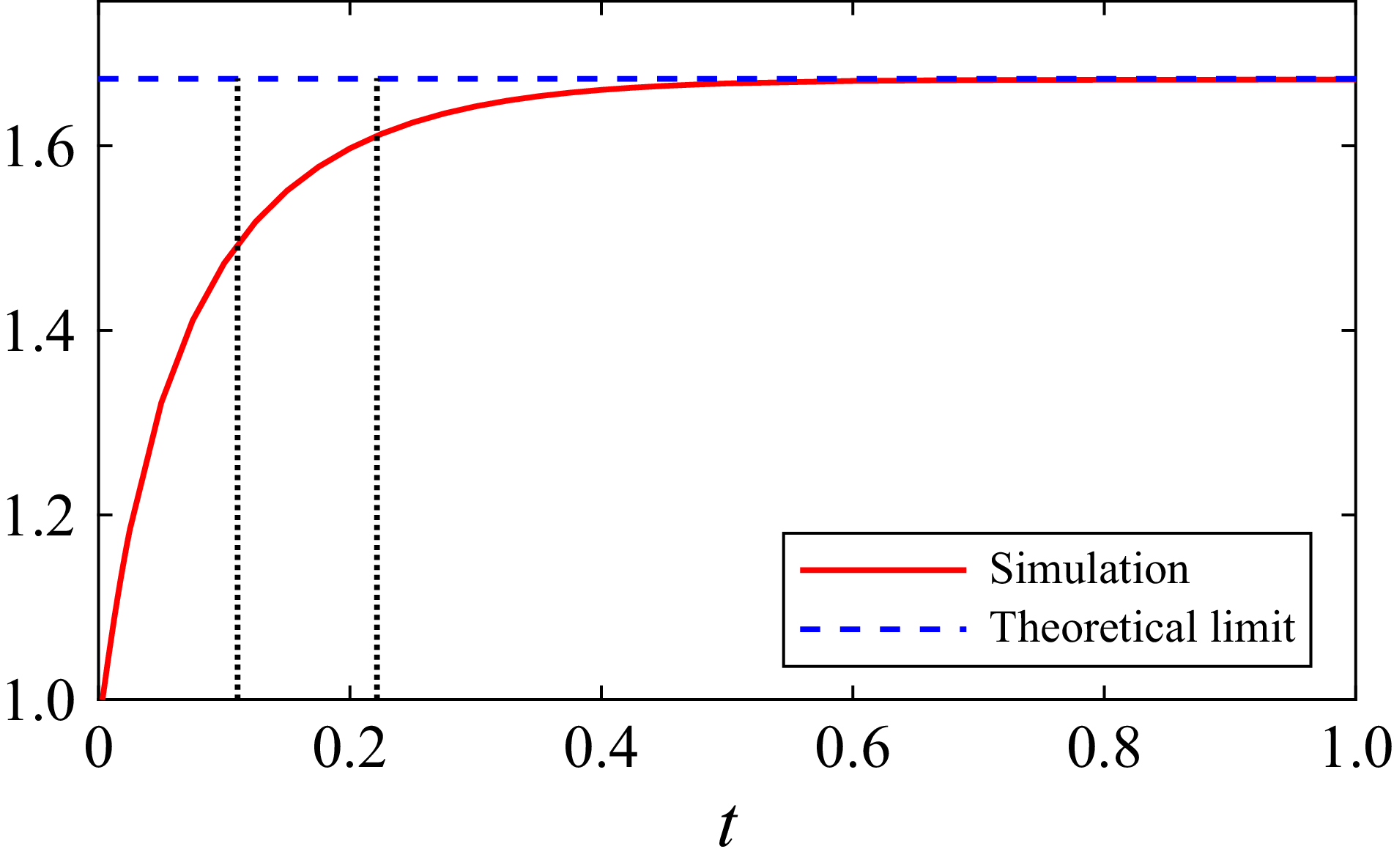


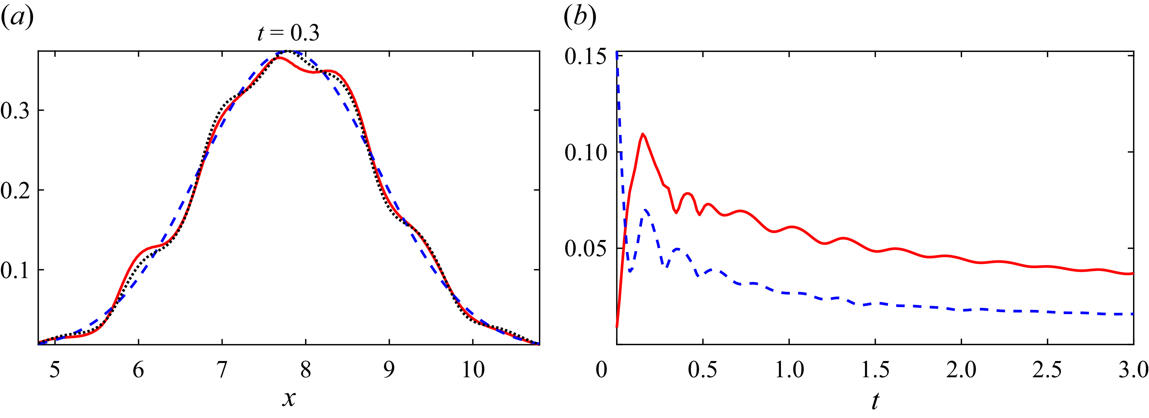


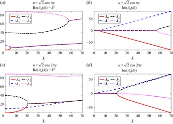

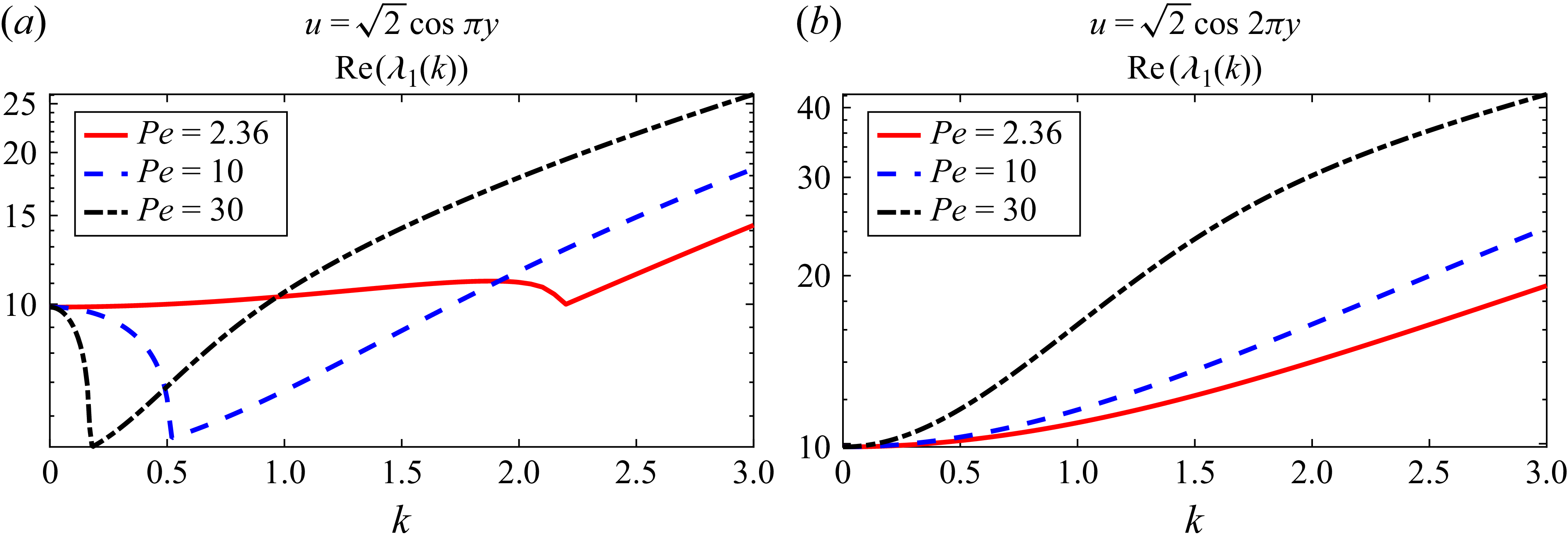


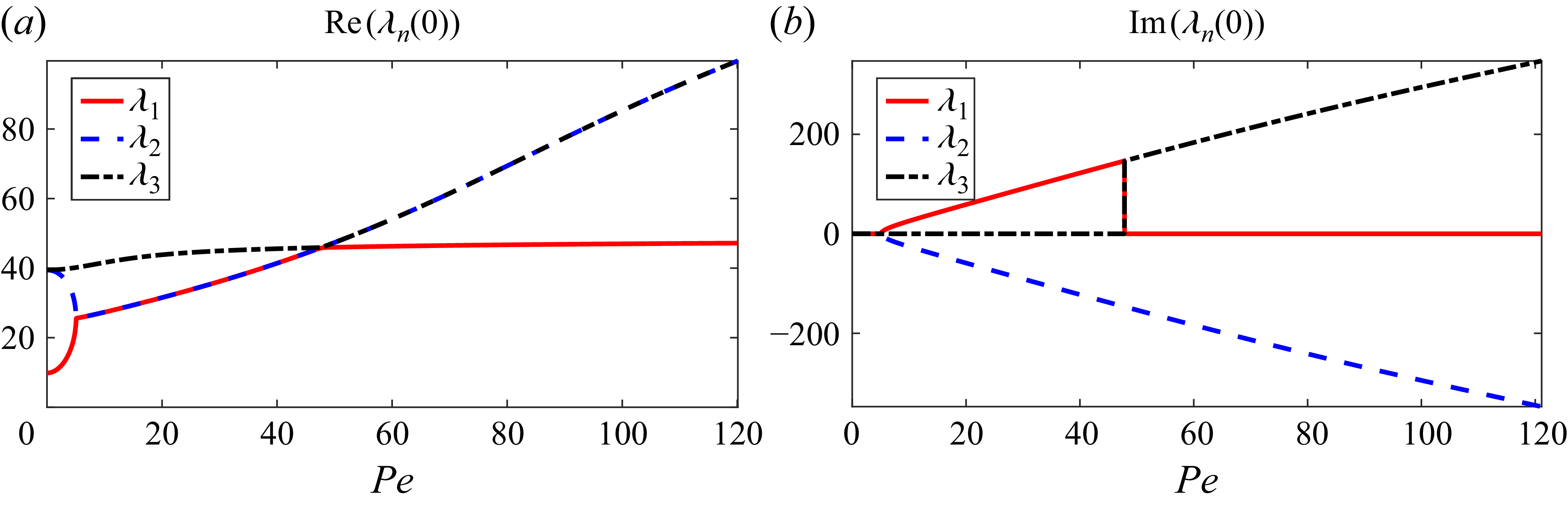


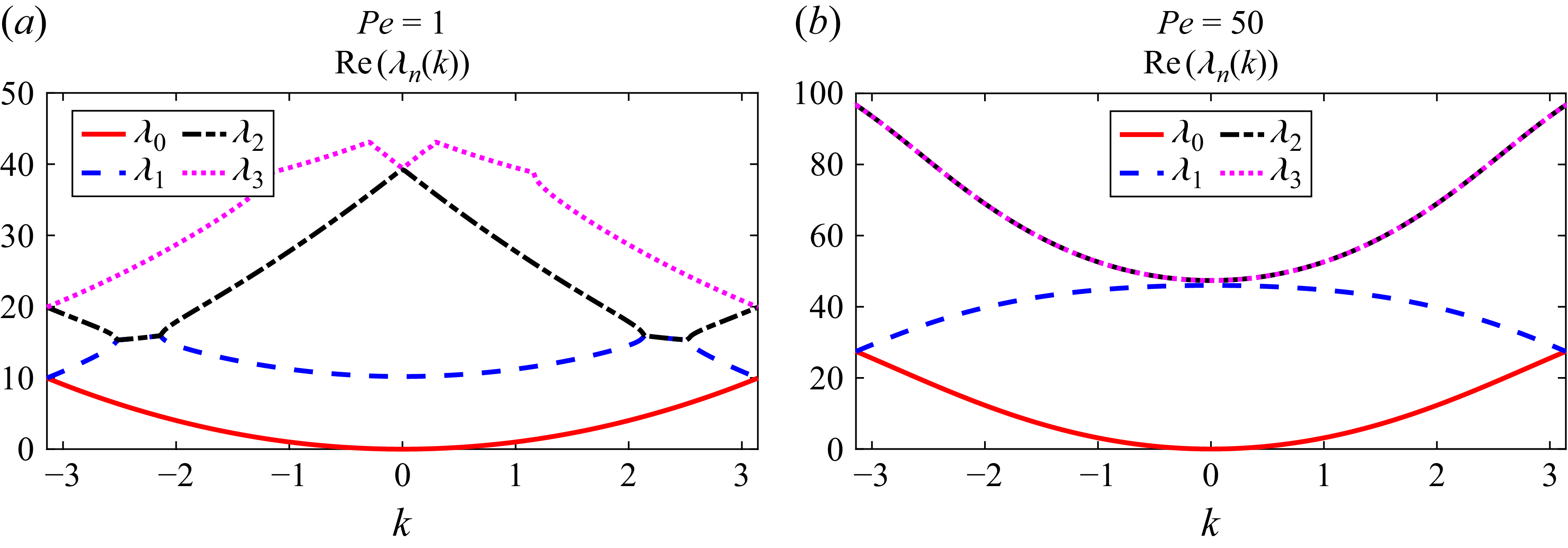


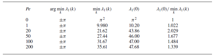
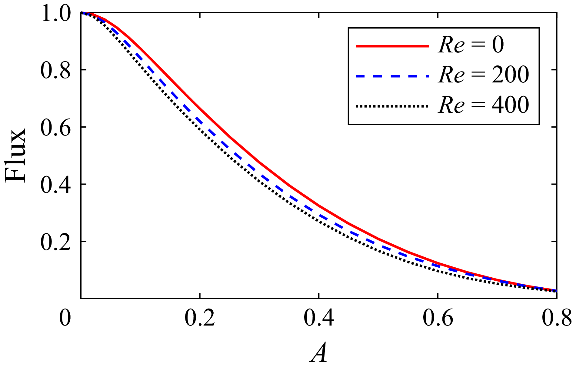


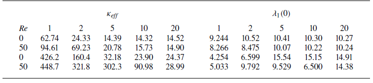


 Open access