


1. Introduction
Discrete tones have been observed in shock-containing jets since the 1950s. These are associated with the screech phenomenon, first studied by Powell (Reference Powell1953a) using schlieren photographs, who suggested that this resonance loop arose from a mechanism involving large-scale structures and upstream-travelling acoustic waves. Such assumptions were used in the development of several resonance models focused on predicting screech frequencies for different jet regimes, and most of them are summarised in recent reviews (Raman Reference Raman1998; Edgington-Mitchell Reference Edgington-Mitchell2019). The seminal works of Merle (Reference Merle1956) and Davies & Oldfield (Reference Davies and Oldfield1962) identified that screech tones associated with axisymmetric disturbances could actually be separated into two stages, A1 and A2, related to different acoustic tones. They also showed the existence of B, D and C modes, relating to flapping and helical disturbances. The A1 to A2 mode staging is unique in that no change in azimuthal mode accompanies the change in tonal frequency; other discontinuities in frequency are accompanied (and presumably driven) by a change in the azimuthal mode  $m$ of screech, in the case of transition from A to B stages, or by a change in the phase relationship between $m=\pm 1$, in the B/D (flapping) to C (helical) stages (Edgington-Mitchell Reference Edgington-Mitchell2019). This property of the A1 and A2 modes has driven efforts to seek alternative explanations for the mechanism behind the frequency change, including different closure mechanisms for the resonance loop (Shen & Tam Reference Shen and Tam2002). However, recent studies have shown that for both the axisymmetric A1 and A2 screech modes, the resonance phenomenon is underpinned by the downstream-travelling Kelvin–Helmholtz (KH) wavepacket and guided, upstream-travelling jet modes (Edgington-Mitchell et al. Reference Edgington-Mitchell, Jaunet, Jordan, Towne, Soria and Honnery2018; Gojon, Bogey & Mihaescu Reference Gojon, Bogey and Mihaescu2018); the change in frequency cannot be explained by a change in the nature of the upstream-propagating wave. The latter belongs to a branch of discrete modes of the stability eigenspectrum associated with a waveguide behaviour of the jet (Tam & Hu Reference Tam and Hu1989), and only becomes discrete at specific (cut-on) frequencies, for which their phase velocity is below the sound speed. Prediction models using this upstream-travelling jet mode are in good agreement with experiments (Mancinelli et al. Reference Mancinelli, Jaunet, Jordan and Towne2019, Reference Mancinelli, Jaunet, Jordan and Towne2021), prevailing over models that consider acoustic waves for resonance closure.
Even though waves can be described using models based on the physics of the problem, such as the vortex-sheet formulation, semi-empirical relations are often used to obtain a wavenumber relationship between upstream- and downstream-travelling waves, such that screech frequencies can be predicted. Tam, Seiner & Yu (Reference Tam, Seiner and Yu1986) followed a different approach, and considered screech as a special case of broadband shock-associated noise. In this framework, as formulated by Tam & Tanna (Reference Tam and Tanna1982), acoustic waves are generated by the interaction between instability waves and the shock-cell structure, which generates sound in directional patterns. Thus, the authors stated that screech could be seen as the limit of this theory when radiation in the upstream direction is considered. Some aspects of this phenomenon were confirmed by Shen & Tam (Reference Shen and Tam2002), whose model predictions using the shock-cell dominant wavenumber were comparable with experiments for the A1 and B modes, even though acoustic waves were used in their predictions. Still, no clear verification of this mechanism was provided for the A2 mode.
The theory developed by Tam & Tanna (Reference Tam and Tanna1982) was verified both experimentally and by linear stability models in the work of Edgington-Mitchell et al. (Reference Edgington-Mitchell, Wang, Nogueira, Schmidt, Jaunet, Duke, Jordan and Towne2021). In this work, the expected wavenumber relation between the different waves in the flow was obtained from the spatial Fourier spectrum of both the dominant proper orthogonal decomposition (POD) and the global stability modes. Nogueira et al. (Reference Nogueira, Jordan, Jaunet, Cavalieri, Towne and Edgington-Mitchell2022) shed light on this underlying energy redistribution mechanism. Their results showed that an absolute instability mechanism induced by the spatial periodicity of the flow is triggered at frequencies similar to the measured screech tones, with associated modes that resemble resonant flow fields obtained from optical diagnoses. The main parameters that define the frequency of the saddle-point in the complex plane are the wavenumbers of the KH and guided jet modes, and the shock-cell wavenumber. This mechanism is expected to be present in all stages of screeching jets.
The main focus of this paper is to provide a clarification on the underlying mechanisms responsible for the generation of A1 and A2 screech modes in a supersonic imperfectly expanded jet. For that, two methods are proposed. First, we study screech generation by analysing the different waves that the flow can support at several streamwise stations. Instead of using semi-empirical relations, or considering a given shock as a reflection point for an incident KH wave (Mancinelli et al. Reference Mancinelli, Jaunet, Jordan and Towne2019, Reference Mancinelli, Jaunet, Jordan and Towne2021), we consider that the upstream-travelling waves are generated by interaction between the Kelvin–Helmholtz wavepacket and the shock-cell structure, as in Tam & Tanna (Reference Tam and Tanna1982). We then analyse the frequency of the saddle-points in the complex plane via spatially periodic linear stability analysis using an analytical flow model. We start by presenting the modelling methods in § 2. In § 3, we describe the experimental set-up for the evaluation of mean flows and sound spectra as a function of ideally expanded Mach number  $M_j$, and in § 4, we show some key characteristics of the shock-cell structure that will distinguish the mechanisms of A1 and A2 screeching modes. Results of the modelling are shown in §5, where the dominance of either screech mode is obtained by analysing the spatio-temporal growth rate of the absolute instability. The paper is closed with conclusions in § 6.
2. Screech-frequency evaluation methods
2.1. Weakest-link model
The first method is similar to the analysis performed in screeching twin-jets by Nogueira & Edgington-Mitchell (Reference Nogueira and Edgington-Mitchell2021). It is based on the shock-cell structure in supersonic jets and on the different waves supported by the flow at each streamwise station. Following the derivations of Tam & Tanna (Reference Tam and Tanna1982) and Shen & Tam (Reference Shen and Tam2002), detailed by Edgington-Mitchell et al. (Reference Edgington-Mitchell, Wang, Nogueira, Schmidt, Jaunet, Duke, Jordan and Towne2021), the interaction between a Kelvin–Helmholtz wavepacket (peak wavenumber  $k_{kh}$) and the shock-cell structure (peak wavenumber $k_{sh}$) transfers energy to specific wavenumbers $k_x$ given by
 \begin{equation} k_x = k_{kh} \pm k_{sh}. \end{equation}
We here consider characterisation of the A1 and A2 modes based on the streamwise evolution of the shock-cell structure and on spatial linear stability analysis around an experimental mean flow. Only the leading shock-cell wavenumber was considered in previous studies, but it is well known that the shock spacing is a function of streamwise position (as shown by Harper-Bourne & Fisher (Reference Harper-Bourne and Fisher1974), see also Tam, Jackson & Seiner Reference Tam, Jackson and Seiner1985; Ray & Lele Reference Ray and Lele2007). As will be seen in § 4, a key element of this work is the inclusion of variation in shock spacing. This variation manifests as secondary peaks in the spectral domain, and these secondary peaks are likewise potential sources of interaction as per (2.1). The inviscid linearised Navier–Stokes equation can be written using matrix operators in a generalised eigenvalue problem form as
 \begin{equation} {\boldsymbol{A}}{\boldsymbol{q}} = k_x {\boldsymbol{B}} {\boldsymbol{q}}, \end{equation}
where the disturbance vector  $\boldsymbol {q}(r)=[ \nu \ u_x \ u_r \ u_\theta \ p]^\mathrm {T}$ includes specific volume, streamwise, radial and azimuthal velocities, and pressure. All variables are considered to have a $\exp ({-\mathrm {i} \omega t + \mathrm {i} k_x x + \mathrm {i} m \theta })$ implicit dependency in this locally parallel framework, and the operators ${\boldsymbol {A}}$ and ${\boldsymbol {B}}$ are dependent on the mean quantities at a fixed streamwise station $x_0$
$x_0$  $\bar {{\boldsymbol {q}}}(x_0,r)=[\bar {\nu } \ U_x \ U_r \ U_\theta \ P]$, on the azimuthal wavenumber and on the radial derivatives. The influence of the mean radial and azimuthal velocities is considered to be negligible for the low Mach numbers analysed herein ( $U_r=U_\theta =0$), and all mean-flow quantities are extracted from experiments, as detailed in § 3. All variables are normalised using the jet diameter $D$, the ambient sound speed $c_\infty$ and the ambient density $\rho _\infty$. Equation (2.2) is solved numerically in MATLAB using a Chebyshev polynomials discretisation (Trefethen Reference Trefethen2000) in the radial direction, with $N_r=250$ points. The mapping developed by Lesshafft & Huerre (Reference Lesshafft and Huerre2007) was used to obtain a higher node density in the shear and core regions of the jet, and boundary conditions were implemented as in the cited work. A sketch of the present method is shown in figure 1(a).
Sketch showing how each wave is computed in the models presented herein. Locally parallel linear stability analysis around a turbulent mean flow (a) and spatially periodic linear stability analysis (b).

In this framework, (2.1) fixes a wavenumber relationship between interacting waves in the flow. The Kelvin–Helmholtz wavepacket is the most amplified coherent structure in these jets. Upstream-travelling waves with wavenumber  $k_{kh}-k_{sh}$ are thus likely to arise with high amplitudes, which makes them a natural candidate to close the resonance phenomenon in these screeching jets. To evaluate the validity of this hypothesis, the following three-step analysis is proposed.
(i) Compute the peak wavenumbers of the shock-cell structure from the mean velocity or pressure fields for each Mach number.
(ii) Use spatial linear stability analysis around the mean velocity field to extract the wavenumber of the Kelvin–Helmholtz mode ( $k_{kh}$) as a function of frequency. The same analysis provides the wavenumbers of the upstream travelling waves, highlighting all $k^-$ waves supported by the flow.
(iii) Compute the intersection between the interaction wave (
$k_{kh}-k_{sh}$) and the branch of upstream-travelling waves supported by the flow, obtained from the eigenspectrum computation at several frequencies. This intersection will provide an estimate of the screech frequency for each Mach number analysed.


While the model described in this section may be useful to predict screech tones when a single mode is at play, it provides no argument for the dominance of different tones when there are multiple competing mechanisms. This is addressed in the next section, where the effect of shock-cell periodicity is explicitly explored.
2.2. Absolute instability analysis
In the model described in the previous section, the periodicity of the flow is considered a posteriori; all wavenumbers are computed assuming a parallel flow, and the energy transfer arising from periodicity is imposed by the resonance condition (as per (2.1)). The model presented in this section considers a periodic flow directly in the stability analysis; the system is linearised around a periodic mean flow in the shape
 \begin{equation} U_x(x,r)=U(r)\left[1+A_{sh} \cos{\left( k_{sh} x \right)}\right], \end{equation}
where  $A_{sh}$, $k_{sh}$ are the shock-cell amplitude and wavenumber. The radial profile of the mean streamwise velocity in each axial station is given by
 \begin{equation} U(r)=M\left[0.5+0.5\mathrm{tanh}\left(0.5\left(\frac{r_j}{r}-\frac{r}{r_j}\right) \frac{1}{\delta}\right)\right], \end{equation}
where  $M=U_j/c_{\infty }$ is the Mach number, $U_j$ and $r_j=0.5D_j$ are the ideally expanded jet velocity and equivalent radius, and $\delta$ is a parameter that characterises the shear layer thickness (see Michalke Reference Michalke1971). This mean flow is periodic by construction, and is considered to be a first approximation of a jet with an embedded shock-cell structure, as shown in figure 1(b). This mean flow periodicity allows us to use the Floquet ansatz, which considers solutions in the shape
 \begin{equation} \boldsymbol{\hat{q}}(x,r) = \boldsymbol{\tilde{q}}(x,r)\mathrm{e}^{\mathrm{i}\mu x}, \end{equation}
where  $\mu =\mu _r+\mathrm {i}\mu _i$ is the Floquet exponent and $\boldsymbol {\tilde {q}}(x,r)$ can be represented using a Fourier series. Replacing (2.5) in the linearised Navier–Stokes system, we can rewrite it as an eigenvalue problem, similar to the locally parallel case:
 \begin{equation} \boldsymbol{\tilde{A}} \boldsymbol{\tilde{q}} = \boldsymbol{\tilde{B}} \mu \boldsymbol{\tilde{q}}. \end{equation}
 The operators  $\boldsymbol {\tilde {A}}$, $\boldsymbol {\tilde {B}}$ are an extension of the locally parallel operators $\boldsymbol {{A}}$, $\boldsymbol {{B}}$ to the periodic case, and they can be found in Nogueira et al. (Reference Nogueira, Jordan, Jaunet, Cavalieri, Towne and Edgington-Mitchell2022). As in the locally parallel case, the solution of the present eigenvalue problem leads to waves that can be classified as stable, unstable or neutral, following the Briggs’ criterion (Briggs Reference Briggs1964; Brevdo, Bridges & Smith Reference Brevdo, Bridges and Smith1996); for instance, downstream-travelling waves will be amplified in space if $\mu _i<0$, and damped if $\mu _i>0$. One of the main differences between the spatially periodic linear stability analysis (SPLSA) and the locally parallel linear stability analysis (LSA) is the shape of the solution: now, instead of having a single wavenumber, each eigenmode is allowed to have energy in wavenumbers following $k_r \pm N k_{sh}$, with $N$ an integer. For that reason, all eigenvalues appear periodically in the complex plane, which causes upstream- and downstream-travelling waves to appear in the same region of the eigenvalue spectrum. As shown by Nogueira et al. (Reference Nogueira, Jordan, Jaunet, Cavalieri, Towne and Edgington-Mitchell2022), these periodicity effects give rise to an absolute instability, where a saddle-point involving the KH and the guided jet mode is observed for complex frequency $\omega _0=\omega _{0r}+\mathrm {i} \omega _{0i}$. The presence of this double-root in the eigenspectrum causes the flow to behave as an oscillator, triggering the screech phenomenon.
Considering the good agreement between the frequencies of the saddle-points and the screech frequencies provided in the cited work, tracking saddles for different Mach numbers can be used as a screech prediction tool. As a means of prediction, this method has the advantage of being both empirically verified and physically justified; it is based on the underlying mechanism of screech generation. Several possible frameworks can be constructed to support such an approach to screech prediction: for example, one could use the expression from Pack (Reference Pack1950) to obtain the main shock-cell wavenumber as a function of Mach number and try to recreate the  $St \times M_j$ plots typical of screech tones (which will also be a function of the shear-layer thickness). In the present work, we follow a slightly different path: instead of using the expression from Pack (Reference Pack1950), we obtain the most energetic wavenumbers of the shock-cell structure from experiments to study the transition between A1 and A2 modes. By analysing the spatio-temporal gain of the absolute instability $\omega _{0i}$, it is also possible to determine which mode will be dominant at each Mach number.
The present eigenvalue problem is solved in Matlab using the Arnoldi method. The domain is discretised in both radial and streamwise directions by using Chebyshev polynomials and Fourier modes, respectively (Weideman & Reddy Reference Weideman and Reddy2000). As in the previous section, radial mapping and boundary conditions are implemented as in Lesshafft & Huerre (Reference Lesshafft and Huerre2007). Considering that the mean flow has an analytical expression, convergence of the relevant modes is achieved by using  $N_r \times N_x=80 \times 31$ in most cases.
3. Experimental methodology
To provide mean velocity fields and to evaluate the different screech frequencies of a round jet, an experimental campaign was conducted at the SUCRÉ (SUpersoniC REsonance) jet-noise facility of the Institut Pprime in Poitiers. The stagnation temperature at the nozzle inlet was kept constant at  $T=295$ K and jet exit variables were estimated using isentropic flow equations. The jet operates in an under-expanded condition, issuing from a convergent nozzle of diameter $D=0.01$ m. In the present study, the stagnation pressure was varied to obtain jets with ideally expanded Mach numbers ranging the interval $M_j=[1,1.3]$, with spacing ${\rm \Delta} M_j = 0.005$. Measurements using an azimuthal array of six microphones were performed at the nozzle exit plane and radial distance $r/D=1$. This allowed decomposition of the near pressure field into azimuthal Fourier modes; because we focus on the A1 and A2 modes, only $m=0$ will be analysed. For more details on the facility and the experiments performed, the reader can refer to Mancinelli et al. (Reference Mancinelli, Jaunet, Jordan and Towne2019).
Particle-image velocimetry (PIV) was performed in this flow for discrete values of  $M_j = 1.080; 1.120; 1.160; 1.220$. The flow was seeded using Ondina oil particles before entering the stagnation chamber, ensuring a sufficient seeding homogeneity. The particles were illuminated by a $2 \times 50$ mJ Nd-YAG laser and the images were recorded with a 4 Mpix CCD camera equipped with a Sigma 105 mm Macro lens. The camera provided a field-of-view of approximately $10 D \times 10 D$. The PIV image pairs were acquired at a sampling rate of 7.2 Hz with a ${\rm \Delta} t$ of 1 $\mathrm {\mu }$s. For each configuration a total of 100 00 image pairs were acquired to obtain well-converged statistics. The images were processed using LaVision's Davis 8.0 software using a multipass iterative correlation algorithm (Willert & Gharib Reference Willert and Gharib1991; Soria Reference Soria1996) starting with an interrogation area of $64\times 64$ pixels and finishing with $16 \times 16$ pixels. The overlap between neighbouring interrogation windows was set at $50\,\%$, leading to a resolution of approximately $2.5$ vectors per millimetre (i.e. 25 vectors per jet diameter) in the measured field. At each correlation pass, a peak validation criterion was used: vectors were rejected if the correlation peak ratio was lower than $1.4$. This value was selected as the minimum acceptable value ensuring validation in the potential regions of the flow while rejecting most of the evident erroneous vectors. Outliers were then further detected and replaced using universal outlier detection (Westerweel & Scarano Reference Westerweel and Scarano2005). The mean pressure and density fields were estimated from the velocity fields using a Crocco–Busemann approximation based on isentropic relations, and a spatial integration method, as described by Van Oudheusden et al. (Reference Van Oudheusden, Scarano, Roosenboom, Casimiri and Souverein2007). All fields were interpolated onto the radial mesh used in the linear stability analysis at the required streamwise position. The mean streamwise velocity fields from PIV and the associated predicted mean pressure fields are shown in figure 2. While the shock cells are already visible in the velocity fields of these jets, they are more clearly visualised in the pressure fields. As expected, both the strength and the spacing of the shocks increase with increasing $M_j$ (as predicted by Pack Reference Pack1950). Furthermore, the shocks are shown to decay further downstream owing to increased mixing in that region, which is also associated with a change in shock-cell spacing (Harper-Bourne & Fisher Reference Harper-Bourne and Fisher1974). This is further explored in the next section.
Sample mean streamwise velocity fields and the associated predicted mean pressure fields for the Mach numbers studied herein: (a)  $U_x$, $M_j=1.08$; (b) $P$,
$P$,  $M_j=1.08$; (c) $U_x$, $M_j=1.12$; (d) $P$,
$P$,  $M_j=1.12$; (e) $U_x$, $M_j=1.16$; (f) $P$,
$P$,  $M_j=1.16$; (g) $U_x$, $M_j=1.22$ and (h) $P$,
$P$,  $M_j=1.22$.

4. Spectral characteristics of the shock-cell structure
The relevance of the dominant shock-cell wavenumbers in the redistribution of energy from the wavepacket to the upstream waves motivates an evaluation of the overall spectral characteristics of the shock-cell structure. Figure 3(a) shows the typical behaviour of  $P_{centre}(x)=P(x,0)-\overline {P(x,0)}$ (shown here for $M_j=1.16$), where the overbar denotes the streamwise mean. The distribution resembles a Gaussian-modulated cosine function, displaying an amplitude peak close to the nozzle and a decay further downstream. The streamwise spatial Fourier transform of this field performed across the whole experimental domain is shown in figure 3(b), where a sharp peak is observed around $k_x D = 10$, followed by secondary peaks at higher wavenumbers. Such behaviour of the Fourier transform of frequency-varying signals is common in other frequency modulated signals, such as chirps and linear time-delayed signals (Cook & Bernfeld Reference Cook and Bernfeld1967), and analytical assessment of such phenomena can be performed using asymptotic methods, such as the method of stationary phase (Murray Reference Murray1984).
Mean pressure at the centreline educed from data and from different fitting functions for  $M_j=1.16$. The streamwise mean was subtracted from $P$ to highlight the oscillatory behaviour. All curves are normalised by their maximum. (a) Mean pressure at the centreline and (b) spatial Fourier transform of $P_{centre}$.

The spectrum of  $P_{centre}$ suggests that the shock-cell structure cannot be represented using a single wavenumber. This is exemplified by fitting two Gaussian-modulated cosine functions to the data: the first has a constant wavenumber $k_{sh}D=9.2138$ and the second has a spatially varying wavenumber $k_{sh}(x)D=9.2138+2.544\times 10^{-5}(x/D)^{6}$. The functions are normalised to have the same maximum amplitude and their overall shape is given by
 \begin{equation} P_{fit}(x)=\exp({-0.1(x/D-1.1)^2}) \cos{(k_{sh} x - 0.4608)}, \end{equation}
where the different coefficients in the above expression are obtained from a least-squares fit of the experimental data at this condition.
Figure 3(a) shows that a fit with a single wavenumber correctly follows the experimental data for  $x/D<4$; for positions further downstream, the wavelength associated with the shock-cell decreases, in agreement with previous studies (Harper-Bourne & Fisher Reference Harper-Bourne and Fisher1974). This decrease in wavelength is correctly captured by the spatially varying wavenumber function, which matches the data quite closely throughout the domain. The effect of the spatial variation of $k_{sh}$ is seen in figure 3(b): while the Gaussian-modulated single-frequency cosine displays a single peak in the spectrum, the streamwise variation leads to the appearance of several secondary peaks in positions that agree well with the experimental data.
The wavenumber spectra for all values of  $M_j$ studied in this work are shown in figure 4, where the presence of secondary peaks is shown to persist throughout the parameter space. The wavenumbers of the two first energetic peaks decay with the increase of $M_j$ (as predicted by Pack Reference Pack1950), but the difference between them is kept approximately constant. Considering that the spatial variation of the shock-cell wavenumber generates new peaks in the spectrum, both first and second peaks will be used for the analyses detailed in § 2. These two wavenumbers will be denoted $k_{sh1}$ and $k_{sh2}$. In the present work, the spatial Fourier transform is obtained without a windowing function, but the addition of a Hanning window does not affect the positions of the primary and secondary shock-cell wavenumbers. A similar behaviour for the shock-cell structure was also observed by Morris & Miller (Reference Morris and Miller2010), but the secondary peaks (not associated with the spatial harmonics) were not explored in depth; because these sub-optimal wavenumbers do not agree with the higher-order wavenumbers predicted by Pack (Reference Pack1950), this previous result suggests that those peaks were actually related to the spatial variation of the shock-cell structure.
Normalised spatial spectrum of the mean pressure field at the centreline as a function of  $M_j$. Experimental datapoints are depicted by crosses.

5. Results
In this section, we evaluate the performance of both models in predicting the screech tone. One should keep in mind that the models differ in the consideration of periodicity; while the first (weakest-link model) uses this assumption to obtain an expression for the resonance condition, the second (absolute instability) imposes periodicity directly in the formulation, and resonance is achieved by the presence of a saddle-point between upstream- and downstream-travelling waves with  $\omega _{0i}>0$. Still, in order for the saddle to occur, both the KH and the guided jet modes should be close to one another in the complex plane. This means that close to the saddle, the wavenumber of the upstream wave $k_r^-$ should follow
 \begin{equation} k_r^-\,{\approx}\, k_{kh} - k_{sh} \end{equation}
for some complex  $\omega$. Comparing (5.1) and (2.1), it is clear that the first model provides a first approximation of the saddle-point position and real frequency. Thus, even though no information about the spatio-temporal growth rate can be obtained using the first model, both models may still lead to similar screech frequency predictions.
As shown by Mancinelli et al. (Reference Mancinelli, Jaunet, Jordan and Towne2021), the phase condition first proposed by Powell (Reference Powell1953b) is automatically fulfilled in the weakest-link model. After algebraic manipulation, equivalent equations are obtained for both Tam & Tanna (Reference Tam and Tanna1982) and Mancinelli et al. (Reference Mancinelli, Jaunet, Jordan and Towne2019) models, with the parameters of the latter chosen such that  $k_{sh}= (2p{\rm \pi} -\phi )/L_s$, which results in the same predictions for both. Furthermore, both phase and gain conditions are satisfied in the absolute instability framework (at least partially) as this mechanism leads to the spatio-temporal growth of disturbances in both directions of the flow. This analysis considers: i) the gain associated with the downstream process (via the growth rate of the KH wave); ii) the efficiency of reflection (by means of the off-diagonal terms in the Navier–Stokes system, as described in Nogueira et al. Reference Nogueira, Jordan, Jaunet, Cavalieri, Towne and Edgington-Mitchell2022) and iii) the efficiency of the upstream process (via the growth rate of the guided jet mode, which is usually considered to be neutral in the resonance analysis). The only process not considered in this framework is the receptivity at the nozzle, which mainly affects screech amplitude (Raman Reference Raman1997). Owing to the lack of this last element, the absolute instability framework differs from the classic definition of a long-range feedback loop, but it may be viewed as a local feedback phenomenon that leads to a resonant behaviour as discussed by Chomaz, Huerre & Redekopp (Reference Chomaz, Huerre and Redekopp1991) and Monkewitz, Huerre & Chomaz (Reference Monkewitz, Huerre and Chomaz1993). In the end, this framework is directly connected to the expected stability characteristics of the flow, and also conforms to the basic elements of the classical description of screech.
One should also be aware that both models are based on linear stability analyses around an experimentally obtained/inspired mean flow. As such, the prediction methods inherit the same limitations of the linear stability framework as described by Beneddine et al. (Reference Beneddine, Sipp, Arnault, Dandois and Lesshafft2016). Still, the present analysis considers either convective instabilities (in the weakest-link model) or absolute instabilities. Keeping in mind that the latter leads to a globally unstable mode and strongly amplified resolvent responses in the vicinity of the resonant frequency, it is expected that the present results are representative of the phenomenon at play.
5.1. Weakest-link model
To perform the spatial linear stability analysis around the mean flow in the locally parallel framework, a streamwise position must be chosen. While the initial amplification and phase velocity of the KH mode is well described by a vortex-sheet model (Michalke Reference Michalke1971), the choice of streamwise position for the calculation of the upstream mode is less obvious. A single position may not be representative of the phenomenon, especially if one considers the changes in frequencies of existence of these waves with increasing  $x$ and the variation in wavenumber of the KH mode. To assess the robustness of the method, a range of streamwise positions from $x/D=0.2$ (very close to the nozzle) up to $x/D=2$ were analysed. The final position was chosen so as to consider the regions of the flow in which the KH mode is unstable for a range of frequencies close to the screech tones; after this position, it becomes harder to identify the marginally unstable downstream-travelling wave among other modes in the spatial spectrum. Thus, the spectra associated with several mean flow positions with respect to the shock-cell structure were analysed. These positions were used to evaluate the overall frequency-wavenumber characteristics of the different waves underpinning screech, an ensemble of tone-frequencies being computed associated with an ensemble of streamwise locations. All results are presented using the Strouhal number $St={\omega D}/{2 {\rm \pi}U_j}$, where $U_j$ is the ideally expanded jet velocity.
An illustration of the method described in § 2.1 is presented in figure 5 for  $x/D=0.2$. As black and pink circles, the dispersion relation of the discrete neutral and stable upstream waves are shown as a function of $St$ for $M_j=1.08$ and $1.16$. These curves are quite similar to those found by Tam & Hu (Reference Tam and Hu1989), Towne et al. (Reference Towne, Cavalieri, Jordan, Colonius, Schmidt, Jaunet and Brès2017), and the region of existence of the neutral modes is roughly in agreement with that provided by a vortex-sheet model (Edgington-Mitchell et al. Reference Edgington-Mitchell, Jaunet, Jordan, Towne, Soria and Honnery2018; Gojon et al. Reference Gojon, Bogey and Mihaescu2018; Mancinelli et al. Reference Mancinelli, Jaunet, Jordan and Towne2019). One should also note that the cut-on frequency (the lowest frequency in which the guided jet mode exists) is slightly lower owing to the presence of a finite thickness shear layer (Mancinelli et al. Reference Mancinelli, Jaunet, Jordan and Towne2021). The stable modes are also shown (in pink) here for completeness, as resonance involving this mode may be possible if it is weakly damped in space (small $|{\rm Im}(k_x)|$) (Towne et al. Reference Towne, Cavalieri, Jordan, Colonius, Schmidt, Jaunet and Brès2017); in the present analysis, all the tones predicted were related to a resonance that includes the neutral modes. The real part of the wavenumbers energised by the interaction of the unstable Kelvin–Helmholtz mode and the shock-cells, i.e. ${\rm Re}(k_{kh} - k_{sh1})$ (blue) and ${\rm Re}(k_{kh} - k_{sh2})$ (red) are also shown. As shown in figure 5(a), the blue symbols intersect the upstream branch at a single frequency; upstream-travelling waves may thus arise as a result of the interaction. For this value of $M_j$, no intersection is found for the red curve, related to the interaction with the second peak of the wavenumber spectrum. This implies that at this condition, interaction wavenumbers that arise when the KH wave interacts with the secondary shock cell mode are not matched by a propagative mode. The jet is therefore unable to guide this wavenumber interaction upstream and resonance does not occur. The effect of varying $M_j$ is shown in figure 5(b), where $M_j=1.16$ was chosen. For this case, the highest and lowest frequencies of existence of the neutral mode occur at lower frequencies and the reduction of the wavenumbers of the shock-cell structure leads to two intersections with the upstream branch. Thus, the model suggests that resonance can be closed at two different frequencies: the first related to an interaction of the wavepacket with $k_{sh1}$ and the second related to an interaction with $k_{sh2}$. It is worth noting that the second interaction occurs close to the maximum frequency of existence of the neutral guided jet mode, hindering the possibility of an interaction with other higher-frequency peaks of the shock-cell structure.
Wavenumbers of the upstream-travelling waves (circles) and wavenumbers forced by the interaction between the Kelvin–Helmholtz mode and the shock-cells (crosses) as a function of Strouhal number for  $x/D=0.2$ and $M_j=1.08$ (a) and $1.16$ (b). The wavenumber of acoustic waves is represented by the dashed line.

Figure 6 gives an overview of the characteristics of the different waves supported by the flow as a function of streamwise station. In figure 6(a,b), the growth rate and wavenumber of the KH mode for  $St=0.65$ (close to the frequencies where tones are observed in the cases studied herein) are shown. As expected, this downstream-travelling mode is stabilised by the increase in shear-layer thickness and is just marginally unstable after $x/D=2$. For that reason, predictions will be focused on that region of the flow. As shown in figure 6(b), the present model allows for variation in phase velocity of both guided jet and KH modes; changes in the latter are usually less than $10\,\%$ as we vary the streamwise position; thus, predictions using a constant phase velocity for the KH mode (as in Powell (Reference Powell1953b), Tam & Tanna (Reference Tam and Tanna1982), Mancinelli et al. (Reference Mancinelli, Jaunet, Jordan and Towne2019) and many others) leads to similar results. Figure 6(c) shows the dependence of the saddle (cut-off) and branch (cut-on) frequencies of the guided jet mode with $x/D$, which define the frequencies of existence of this wave for each Mach number. Interestingly, the guided jet mode is much more sensitive to the variations in the mean flow induced by the shock-cell structure. Both branch and saddle points vary following the minima and maxima of the shock cells, keeping the difference between the maximum and minimum frequencies in which the flow supports this neutral wave approximately constant with $x/D$; still, these changes in cut-on/off frequencies lead to changes in screech frequency predictions. This is shown in figure 6(d), where both A1 and A2 tones are predicted as a function of streamwise position. Overall, only small variations in the predicted frequencies are observed with the increase of $x/D$, confirming the robustness of the method. For $M_j=1.08$, no intersection is found with the secondary peak of the shock-cell structure, and only A1 tones are predicted. At higher Mach numbers, both A1 and A2 tones are predicted for a range of streamwise positions. Two cases stand out in figure 6(d): the A2 predictions for $M_j=1.12$ and the A1 predictions for $M_j=1.22$. The former displays a continuous small spatial region in which the A2 mode is supported, which is indicative of the transition region between A1 and A2; this would mark the start of the A2 tones in the acoustic spectrum. The latter, however, displays some sparse points in space in which resonance would be sustained. Considering that the resonant mode is spatially spread (Edgington-Mitchell et al. Reference Edgington-Mitchell, Wang, Nogueira, Schmidt, Jaunet, Duke, Jordan and Towne2021), this suggests that A1 resonance may not be supported at this Mach number.
Characteristics of the different waves supported by the flow as function of streamwise position for the several  $M_j$ studied herein. Growth rates (a) and wavenumbers (b) of the KH mode for $St=0.65$, Strouhal number of branch ( $\times$) and saddle ( $+$) points of the neutral guided jet mode (c) and the Strouhal numbers predicted by the weakest-link model as function of $x/D$ for both A1 ( $\square$) and A2 ( $\circ$) modes (d).

The comparison between the streamwise average of the frequencies predicted for each  $M_j$ by the method and the experimental power spectral density (PSD) for the different $M_j$ is shown in figure 7. Interaction of the Kelvin–Helmholtz mode with the main peak of the cell spectrum ( $k_{sh1}$), in blue, produces an accurate prediction of the A1 screech frequencies for all cases where this mode is expected to be dominant ( $M_j<1.16$). As mentioned previously, the A1 mode ceases to exist for higher values of $M_j$ owing to a decrease of the cut-on frequency of the discrete guided jet wave with increase of $M_j$. A similar trend is obtained for the A2 mode (red): for $M_j \geq 1.12$, where this mode dominates, the model leads to frequencies quite close to the peaks in the experiments. No intersection is found for the lowest value of $M_j$ for any of the streamwise stations analysed here, which highlights that this mode can only exist for higher Mach number, as expected for the A2 resonance. Figure 7 also shows the bounds of existence of neutral waves from Mancinelli et al. (Reference Mancinelli, Jaunet, Jordan and Towne2021), obtained from a vortex-sheet (VS) model; as expected, most frequencies predicted by the present model are inside the region of existence of the neutral mode from such a model. As mentioned earlier, compared with the VS, the branch points of the guided jet mode occur for lower frequencies in the present analysis due to the inclusion of a finite shear-layer thickness, as also observed by Mancinelli et al. (Reference Mancinelli, Jaunet, Jordan and Towne2021). One should also note that the base flow profiles used in the present analysis differ from those used in the cited reference, which could lead to differences in branch and saddle point positions.
Comparison between the frequencies predicted by the model (symbols) and the PSD map of a screeching jet as a function of  $M_j$. Average Strouhal number of the predictions of the A1 and A2 modes are depicted by blue and red curves, respectively. Yellow dashed/continuous lines represent the cut-on/off frequencies from a vortex-sheet model (taken from Mancinelli et al. Reference Mancinelli, Jaunet, Jordan and Towne2021).

Some limitations of the model can also be observed when only wavenumber and frequency are considered. The most striking one is that the model does little to explain the selection of either A1 or A2 at Mach numbers where the flow can support both. The spatially periodic analysis addresses this limitation by considering the growth rates associated with each resonance loop. This analysis is performed in the next section.
5.2. Absolute instability analysis
We now turn to the spatially periodic analysis. As described by Nogueira et al. (Reference Nogueira, Jordan, Jaunet, Cavalieri, Towne and Edgington-Mitchell2022), the periodicity of the spatial spectrum induced by the shock-cell structure causes guided jet and KH modes to be in the same region of the spectrum. If the shock-cell amplitude is non-zero, a saddle-point between these two modes can be formed. In this section, we track the saddle frequencies as a function of  $M_j$ for all the four cases where experimental results are available. As in Nogueira et al. (Reference Nogueira, Jordan, Jaunet, Cavalieri, Towne and Edgington-Mitchell2022), the shock-cell strength is kept as $A_{sh}=0.02$, but results are roughly insensitive to this parameter; in fact, saddles are found until the limit $A_{sh} \to 0$, where dominant and suboptimal saddles coalesce and no absolute instability is observed. This suggests that both $k_{sh1}$ and $k_{sh2}$ may be able to close the resonance loop. This is also in agreement with the long-range resonance model (Mancinelli et al. Reference Mancinelli, Jaunet, Jordan and Towne2021). In that model, the shock-cell mode strength fixes the reflection coefficient amplitude, and while this has an effect, the spatial amplification of the KH mode is a more important parameter. To evaluate the sensitivity of these results to the shear-layer thickness, $\delta$ was chosen as $0.15$, $0.175$ and $0.20$ for all values of $M_j$ (consistent with the analysis of Nogueira et al. Reference Nogueira, Jordan, Jaunet, Cavalieri, Towne and Edgington-Mitchell2022). All saddles were computed using the method proposed by Monkewitz (Reference Monkewitz1988). As an analytical approximation for a shock-containing mean flow is used in this analysis, it is useful to check if these values are representative of the experimental mean flow. For this purpose, a least-squares fit of (2.4) to the experimental data was performed, so that the values of $r_j$, $M$ and $\delta$ could be approximated as a function of $x/D$. The results for $M$ and $\delta$ are shown in figure 8(a,b), where the Mach number computed from $M_j$ is also shown. The Mach number has an oscillatory behaviour induced by the shock cells, but the the expression $U_j/c_\infty$ captures well the streamwise average in the region analysed. From figure 8(b), the values of $\delta$ chosen in this analysis are equivalent to a region between $x/D=1.3$ and $2.2$, which is also consistent with most regions where A1 and A2 tones are observed in the weakest-link model.
Parameters  $M$ (a) and $\delta$ (b) obtained from a least-squares fit of (2.4) to the experimental data as a function of $x/D$. Dashed lines indicate the Mach number $U_j/c_\infty$ computed from experiments and used in this analysis.

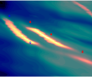
To exemplify the phenomenon at play, figure 9 shows the eigenspectrum close to the saddle point for several Strouhal numbers. This is done for the imaginary frequency of the most unstable saddle, with  $M_j=1.12$ and $\delta =0.20$. In figure 9(a), the first shock-cell wavenumber ( $k_{sh1}$) is used and $k_{sh2}$ is used in figure 9(b). In both cases, Kelvin–Helmholtz modes (indicated in red) travel from left to right, while guided jet modes (indicated in blue) travel from right to left, and the acoustic modes were removed from the spectrum for clarity. These plots show that the trajectory of one mode is modified by the presence of the other in such a way that both are attracted to a single point in the spectrum; after reaching that point, the modes are repelled away, eventually returning to their original trajectories as the distance from the saddle is increased. Following Brevdo et al. (Reference Brevdo, Bridges and Smith1996), the resulting double root at the saddle point will grow both downstream and upstream, causing the jet to behave as an oscillator, triggering resonance.
Eigenspectrum of SPLSA close to the saddle point for  $M_j=1.12$ and $\delta =0.2$: (a) modes for $k_{sh}=k_{sh1}$, $\omega _{0i}=0.223$ and $0.627< St<0.633$ and (b) modes for $k_{sh}=k_{sh2}$, $\omega _{0i}=0.057$ and $0.733< St<0.739$. Arrows indicate the direction in which each mode travels in the eigenspectrum for increasing $St$.
$St$.

The same process is carried out for the other values of  $M_j$ and $\delta$, and the Strouhal number of the saddles are shown in figure 10. Overall, the predictions align well with the tones observed in the near-field, with errors of less than $10\,\%$ in Strouhal number. Deviations from the predicted values are expected for some reasons: first, the exact screech frequency is facility dependent, to some extent (see, for example Gojon et al. Reference Gojon, Bogey and Mihaescu2018), and deviations of this magnitude could be expected if results from different laboratories are compared. As the present prediction is only based on the wavenumber of the shocks (which is roughly insensitive to the external contours of the nozzle and other details of the facility, as it comes from the solution of Pack Reference Pack1950), it could be compared to any facility; thus, it may be considered as a reference value for this case. Second, it is likely that the actual equivalent ideally expanded jet profile is different from expression (2.4), which could change the predictions slightly. Furthermore, even though SPLSA includes a surrogate for the shock-cell in the model, it does not account for effects such as the jet spreading and the streamwise decay of the shocks; these effects might also be at play in such a way to decrease the frequency associated with the resonance phenomenon. Considering the simplicity of the model, the level of agreement for both A1 and A2 tones is still rather remarkable.
Comparison between the frequencies of the saddle-points from SPLSA (symbols) and the PSD map of a screeching jet as a function of  $M_j$. Symbols are for $\delta =0.15$ ( $\triangle$), $\delta =0.175$ ( $\times$) and $\delta =0.20$ ( $\circ$).

Figure 10 indicates that the Strouhal number of the saddle is not substantially modified by variations in  $\delta$. However, as shown in figure 11, the growth rate of the absolute instability is severely affected by that parameter. For the first Mach number and $k_{sh}=k_{sh1}$, saddles are found for all values of $\delta$, and $\omega _{0i}$ decreases with increasing shear-layer thickness (which also occurs for all other cases). However, for $M_j=1.12$, no saddle is observed for $\delta =0.15$, as the KH mode crosses the acoustic branch before the guided jet mode becomes cut-on. By increasing the shear-layer thickness, the cut-on frequency decreases and the saddle is recovered. A similar trend on the effect of the shear layer thickness in these waves was also observed by Tam & Ahuja (Reference Tam and Ahuja1990) and more clearly by Mancinelli et al. (Reference Mancinelli, Jaunet, Jordan and Towne2021) (who also used a finite thickness model) and numerically by Bogey & Gojon (Reference Bogey and Gojon2017). This suggests that this Mach number is around the end of the A1 branch and that further increase in $M_j$ will lead to the cessation of that tone. This is confirmed by the analysis of $M_j=1.16, 1.22$, where no A1 saddle is observed for all $\delta$. If $k_{sh}$ is chosen as $k_{sh2}$ (A2 mode), analysis of the eigenspectrum shows that, for $M_j=1.08$, the KH mode never approaches the upstream branch sufficiently to allow for an interaction – for this case, $k_{sh2}$ is too high to allow for an interaction. For $M_j \geq 1.12$, where saddles are found for all values of $\delta$, the same trend of decreasing $\omega _{0i}$ with increasing $\delta$ is observed. It is also shown that the spatio-temporal growth rate ( $\omega _{0i}$) of A1 modes increases rapidly with increasing $M_j$ (note that $A_{sh}$ is kept constant). This agrees with the trend of increasing amplitude of the screech tone with increasing Mach number in the experiments, which suggests that there may be a connection between $\omega _{0i}$ and the final amplitude of the resonant mode. The same is observed for the A2 modes, but the variation in $\omega _{0i}$ is less steep than for the A1 modes. Interestingly, the model predicts an absolute instability for both A1 and A2 modes for $M_j=1.12$, as in the experiments. For this Mach number, the growth rates of the A1 mode are much greater than those of A2 (see also figure 9), suggesting that this mode may be dominant in experiments. This is also in line with the trend observed in the near-field spectrum, where the A1 peak is greater than that of A2.
Imaginary part of the saddle-point frequency as function of  $M_j$ for several values of $\delta$. Both A1 and A2 saddles are shown.

Thus, the spatially periodic analysis provides a clear explanation for several features of the screech tone, including the appearance of the A1 tone (based on the distance between KH and guided jet modes in the periodic spectrum) and its cut-off behaviour for increasing  $M_j$. Consideration of the suboptimal shock-cell wavenumber in the analysis allows for the identification of A2 tones; by comparing the growth rates associated with the saddle-points of both tones, we are able to predict which tone will be dominant for each Mach number. The model also explains why the tone amplitudes increase with $M_j$. Even though all these features are well captured by the model, it also predicts highly amplified A2 tones for $M_j=1.22$, which has a low amplitude axisymmetric peak. Again, this may arise from the characteristics of the facility or the fact that the jet is not exactly a spatially periodic system.
Results from both models provide evidence that the discrete jumps in frequency of axisymmetric tones are associated with discrete peaks of the Fourier spectrum of the shock-cell structure. At first, one could also expect to observe equivalent A3 tones in the spectrum if the third peak of the shock cells was considered. For the lower  $M_j$ cases studied herein, the interaction with this third peak could potentially occur if we considered the stable (rather than neutral) guided jet modes. However, in that case the associated gain of the resonance would be considerably smaller than the A2 mode. For the $M_j=1.22$ case, interactions with the neutral mode may be observed at a few early streamwise positions using the weakest-link model, with an average prediction of $St=0.63$. A similar trend is seen in the absolute instability framework: as in the A1–A2 transition, a lower spatio-temporal growth rate is observed for the possible A3 mode ( $\omega _{0i} \approx 0.31$, calculated for $\delta =0.15$, with $St_{saddle} \approx 0.65$). However, as shown in figure 10, the axisymmetric resonant mode has a much lower amplitude in experiments for this condition; thus, considering that the amplitude of the A2 mode is already small, the amplitude of the A3 mode for this case would be virtually negligible. At these higher $M_j$, it is expected that the resonance associated with $m=1$ disturbances (B mode) will be dominant, thus masking the axisymmetric tones because these resonance loops are usually mutually exclusive (Mancinelli et al. Reference Mancinelli, Jaunet, Jordan and Towne2019).
6. Conclusions
The present manuscript proposes a closure mechanism for the A1 and A2 screech modes based of the most energetic wavenumbers associated with the shock-cell structure. Two models are used to evaluate the hypotheses: the first (weakest-link model) is based on the different waves supported by the flow, and the interaction between wavepackets and the shock-cell structure, considered here as a wave in the mean flow (Tam & Tanna Reference Tam and Tanna1982; Shen & Tam Reference Shen and Tam2002). Considering that the energy is extracted from the mean flow mainly by the Kelvin–Helmholtz mode in this framework owing to the instability mechanism, the interaction between the wavepacket and the shocks will lead to a redistribution of energy, and other wavenumbers will be energised. At frequencies where the wavenumbers of upstream-travelling waves supported by the jet coincide with this interaction wavenumber, a necessary condition for resonance is achieved, and the jet may screech. It is worth highlighting that this is not a sufficient condition for screech, and that reflection/receptivity processes are not accounted for in the model. Still, screech tones can be predicted fairly well, which suggests that other necessary conditions may be identically satisfied in the jet. Results of the screech prediction method using the first and second peak wavenumbers of the shock-cell structure are in good agreement with experiments for a range of streamwise positions used in the locally parallel analysis for both A1 and A2 modes, in the frequency range of dominance of each mode.
The second model considers a system linearised around a periodic mean flow. Eigenmodes related to the different waves supported by the system are obtained using the Floquet ansatz; owing to the periodicity of the spectrum, upstream- and downstream-travelling modes are found in the same region of the spectrum, allowing for interaction. Unstable saddle-points ( $\omega _{0i}>0$) involving the KH and the guided jet modes are observed for all values of $M_j$ studied herein, at Strouhal numbers very close to where tones are found in the near-field spectrum, which supports that screech is caused by this absolute instability mechanism. The model is capable of predicting the cut-on and cut-off behaviour of both A1 and A2 modes (computed using the optimal and first sub-optimal shock-cell wavenumbers, respectively), and also provides a reasoning for the dominance of either A1 or A2 where both modes are supported.
These results support the hypothesis that the interaction between wavepackets and shocks in the ‘weakest-link’ framework, formulated by Tam et al. (Reference Tam, Seiner and Yu1986), is a crucial part of the resonance mechanism. In fact, the conditions in which the cited framework were derived are actually very similar to the conditions for the occurrence of a saddle point, as highlighted in (5.1), which indicates that the physical argument of energy transfer is actually achieved by means of an absolute instability in the flow. Thus, the weakest-link model may be viewed as a first approximation of the absolute instability; similarly, the absolute instability captures some of the elements of the global stability analysis, which provides one of the most accurate representations of the resonant mode in screeching jets (Beneddine, Mettot & Sipp Reference Beneddine, Mettot and Sipp2015; Edgington-Mitchell et al. Reference Edgington-Mitchell, Wang, Nogueira, Schmidt, Jaunet, Duke, Jordan and Towne2021). The agreement of both models with experimental data for both A1 and A2 modes suggests that the A2-screech phenomenon occurs as a consequence of the spatial variation of the wavenumber of the shock-cell structure, a result that has not been shown before. This also suggests why theoretical models for the prediction of the A1–A2 mode staging have generally found little success; most models for jet screech do not consider the effect of spatial variation in the shock structure; in Mancinelli et al. (Reference Mancinelli, Jaunet, Jordan and Towne2019), this is considered inadvertently by different choices of the model parameters, but here it is considered directly from the spatial spectrum of the shock-cell structure. In the cited model, generation of upstream waves is considered to occur at a given streamwise position, at which interaction between the KH wavepacket and the shock cell would lead to reflected and transmitted waves. In the present model, instead of considering the upstream wave as generated by reflection at a given position, we consider the shock-cell pattern as a wave embedded in the time-averaged mean flow, whose interaction with other structures in the flow leads to the generation of upstream-travelling waves. As shown by Mancinelli et al. (Reference Mancinelli, Jaunet, Jordan and Towne2021), both models should provide the same predictions for the right choice of parameters, even though they are derived using different assumptions. The weakest-link model, like the complex-frequency model, addresses one of the limitations of the neutral-mode model, namely the multiple screech tone predictions for different choices of parameters. In the present model, all predictions are performed using the mean flow characteristics, and the parameters  $L_s$, $p$ and $\phi$ are replaced by $k_{sh1}$ and $k_{sh2}$. This leads to a lower variability of the prediction results, as all resonance predictions are based solely on the mean flow characteristics. Also, in the current framework, dominance of either A1 and A2 modes can be explained by the relative growth rates of each mode at the predicted screech frequency. These conclusions are of relevance not only in providing understanding on the screech phenomenon, but can also be used to design models for screech prediction in other flow configurations.
Funding
This work was supported by the Australian Research Council through the Discovery Project scheme: DP190102220. M.M. acknowledges the support of Centre National d‘Études Spatiales (CNES) under a post-doctoral grant.
Declaration of interests
The authors report no conflict of interest.


 Open access