


1. Introduction
Laminar–turbulent transition in confined shear flows remains a central problem in fluid mechanics because of its fundamental significance and its broad engineering applications. In channel flows, the pressure gradient required to sustain turbulence is substantially larger than that required for laminar motion, making accurate prediction of transition essential for design and operation.
In several canonical confined flows, classical linear stability theory has failed to account for the observed transition. Plane Couette flow and Hagen-Poiseuille flow are predicted to be linearly stable at all Reynolds numbers (Drazin & Reid Reference Drazin and Reid2004), yet experiments show transition at moderate Reynolds numbers. Even in plane Poiseuille flow, for which linear theory predicts a critical Reynolds number $Re_c=5772.22$
(Orszag Reference Orszag1971) (where
$Re_c=5772.22$
(Orszag Reference Orszag1971) (where $Re_c$
is based on the half-channel height and the centreplane velocity), transition is observed experimentally at substantially lower Reynolds numbers. These discrepancies have motivated extensive research on subcritical transition and nonlinear disturbance growth in fully developed channel flows.
$Re_c$
is based on the half-channel height and the centreplane velocity), transition is observed experimentally at substantially lower Reynolds numbers. These discrepancies have motivated extensive research on subcritical transition and nonlinear disturbance growth in fully developed channel flows.
In contrast, considerably less attention has been given to the entrance region of a channel, where the velocity profile and pressure gradient vary in the streamwise direction. This spatial development fundamentally alters both the base flow and the mechanisms by which disturbances evolve. Since the laminar entrance length grows linearly with the bulk Reynolds number $Re_b$
(based on the half-channel height) for
$Re_b$
(based on the half-channel height) for $Re_b \gt 100$
(Durst et al. Reference Durst, Ray, Ünsal and Bayoumi2005), it can extend over a very long downstream distance at high Reynolds numbers. Channel-entrance flow has indeed been experimentally maintained laminar up to
$Re_b \gt 100$
(Durst et al. Reference Durst, Ray, Ünsal and Bayoumi2005), it can extend over a very long downstream distance at high Reynolds numbers. Channel-entrance flow has indeed been experimentally maintained laminar up to $Re_b \gt 5000$
in a channel of length 821.9 half-heights (Nishioka et al. Reference Nishioka, Iid and Ichikawa1975). It is however still unclear how vortical disturbances amplify nonlinearly and evolve along this long spatially developing region. In this paper, we thus aim to investigate the flow in the entrance region of a channel, with particular focus on how entrained vortical disturbances grow nonlinearly and evolve downstream.
$Re_b \gt 5000$
in a channel of length 821.9 half-heights (Nishioka et al. Reference Nishioka, Iid and Ichikawa1975). It is however still unclear how vortical disturbances amplify nonlinearly and evolve along this long spatially developing region. In this paper, we thus aim to investigate the flow in the entrance region of a channel, with particular focus on how entrained vortical disturbances grow nonlinearly and evolve downstream.
We review the relevant studies on stability and transition in fully developed channel flows in § 1.1 and in channel-entrance flows in § 1.2. We discuss the boundary-region framework in § 1.3 and outline the objectives of the present study in § 1.4.
1.1. Fully developed channel flow
The linear stability analysis of fully developed channel flow leads to the Orr–Sommerfeld and Squire equations with homogeneous boundary conditions at the channel walls. The Orr–Sommerfeld equation was initially solved by asymptotic methods (Heisenberg Reference Heisenberg1924; Lin Reference Lin1946; Shen Reference Shen1954; Stuart Reference Stuart1963) and later by numerical methods (Thomas Reference Thomas1953; Grosch & Salwen Reference Grosch and Salwen1968; Orszag Reference Orszag1971). The critical Reynolds numbers $Re_c$
obtained in these studies all lie between 5000 and 6000. Experimental studies of laminar–turbulent transition in fully developed channel flow date back to Davies & White (Reference Davies and White1928), who conducted a series of measurements in a rectangular water channel with a width–height aspect ratio ranging from 37 to 165. The transitional Reynolds number was found to be
$Re_c$
obtained in these studies all lie between 5000 and 6000. Experimental studies of laminar–turbulent transition in fully developed channel flow date back to Davies & White (Reference Davies and White1928), who conducted a series of measurements in a rectangular water channel with a width–height aspect ratio ranging from 37 to 165. The transitional Reynolds number was found to be $Re_b=1440$
for channels with aspect ratios larger than 70. Subsequent investigations by Patel & Head (Reference Patel and Head1969), Kao & Park (Reference Kao and Park1970) and Carlson, Widnall & Peeters (Reference Carlson, Widnall and Peeters1982) observed transition for
$Re_b=1440$
for channels with aspect ratios larger than 70. Subsequent investigations by Patel & Head (Reference Patel and Head1969), Kao & Park (Reference Kao and Park1970) and Carlson, Widnall & Peeters (Reference Carlson, Widnall and Peeters1982) observed transition for $Re_b\lt 3000$
. The deviation of experimental observations from theoretical predictions arises from the subcritical nature of transition in the channel flow. The experimental measurements performed by Nishioka et al. (Reference Nishioka, Iid and Ichikawa1975) and Nishioka, Honda & Kamibayashi (Reference Nishioka, Honda and Kamibayashi1981) demonstrated the downstream development of disturbances triggered by a vibrating ribbon in the fully developed region. The nonlinear subcritical instability occurred when the disturbance amplitude exceeded a certain threshold, in agreement with theoretical predictions (Herbert Reference Herbert1980, Reference Herbert1983a
). A rich review of early results on channel-flow stability can be found in the Ph.D. thesis by Pugh (Reference Pugh1988).
$Re_b\lt 3000$
. The deviation of experimental observations from theoretical predictions arises from the subcritical nature of transition in the channel flow. The experimental measurements performed by Nishioka et al. (Reference Nishioka, Iid and Ichikawa1975) and Nishioka, Honda & Kamibayashi (Reference Nishioka, Honda and Kamibayashi1981) demonstrated the downstream development of disturbances triggered by a vibrating ribbon in the fully developed region. The nonlinear subcritical instability occurred when the disturbance amplitude exceeded a certain threshold, in agreement with theoretical predictions (Herbert Reference Herbert1980, Reference Herbert1983a
). A rich review of early results on channel-flow stability can be found in the Ph.D. thesis by Pugh (Reference Pugh1988).
Since modal stability theory cannot fully explain the laminar–turbulent transition in fully developed channel flow, attention shifted to non-modal stability theory (Gustavsson Reference Gustavsson1991; Reddy & Henningson Reference Reddy and Henningson1993). A common approach to the non-modal stability problem is to identify the optimal disturbances that maximise amplification over all possible initial conditions. Butler & Farrell (Reference Butler and Farrell1992) showed that linearly stable three-dimensional disturbances in fully developed laminar channel flow can undergo transient growth before ultimately decaying. These optimal disturbances were found to have zero streamwise wavenumber and take the form of streamwise vortices, which evolve into streaks of high or low streamwise velocity. Optimal disturbances have also been computed in turbulent channel flows by Butler & Farrell (Reference Butler and Farrell1993), del Álamo & Jiménez (Reference del Álamo and Jiménez2006) and Pujals et al. (Reference Pujals, García-Villalba, Cossu and Depardon2009).
Experimental observations of transitional and turbulent wall-bounded flows have revealed the existence of coherent structures in the form of organised patterns of vorticity that persist in both time and space. The significance of coherent structures in turbulent transport processes has driven investigations aimed at finding distinct solutions to the Navier–Stokes equations that capture the characteristics of these structures (Graham & Floryan Reference Graham and Floryan2021). These solutions are now known as exact coherent structures (ECS). Following the idea of the self-sustained mechanism (Hamilton, Kim & Waleffe Reference Hamilton, Kim and Waleffe1995; Waleffe Reference Waleffe1997), Waleffe (Reference Waleffe1998) discovered three-dimensional nonlinear travelling-wave solutions in free-slip plane Poiseuille flow by taking steady states in the free-slip plane Couette flow as starting points. These solutions were later extended to travelling-wave solutions in plane Poiseuille flow by homotopy from free-slip to no-slip boundary conditions (Waleffe Reference Waleffe2001, Reference Waleffe2003). The plane Poiseuille flow investigated by Waleffe was a half-Poiseuille flow with the upper wall corresponding to the centreplane of a full plane Poiseuille flow. The close resemblance between the profiles of half-Poiseuille flow and plane Couette flow made the homotopy possible. These solutions are remarkably similar to the coherent structures observed in the near-wall region of a fully developed turbulent channel flow and also capture the most important statistical features of turbulence. Other families of ECS in plane Poiseuille flow (e.g. periodic-like, mirror-symmetric, hairpin-like and localised) were found by other researchers (e.g. Toh & Itano Reference Toh and Itano2003; Nagata & Deguchi Reference Nagata and Deguchi2013; Zammert & Eckhardt Reference Zammert and Eckhardt2014; Gibson & Brand Reference Gibson and Brand2014; Wall & Nagata Reference Wall and Nagata2016; Shekar & Graham Reference Shekar and Graham2018; Yang, Willis & Hwang Reference Yang, Willis and Hwang2019; Engel et al. Reference Engel, Ashtari, Schneider and Linkmann2025). Further research work is needed to establish how these structures become unstable and break down to the turbulent regime.
1.2. Channel-entrance flow
The discrepancies between theoretical predictions and experimental observations in fully developed channel flow have drawn attention to the disturbances in the entrance region, as a likely cause of the failure of classical stability theory (Herbert Reference Herbert1984a , Reference Herbertb ). Research efforts first focused on the computation of the velocity and pressure distributions of the laminar entrance flow (Bodoia & Osterle Reference Bodoia and Osterle1961; Sparrow, Lin & Lundgren Reference Sparrow, Lin and Lundgren1964; Van Dyke Reference Van Dyke1970; Fang & Saber Reference Fang and Saber1987; Sadri & Floryan Reference Sadri and Floryan2002). Building on these studies of the base flow, subsequent investigations turned to its stability characteristics.
Linear stability analysis of symmetric disturbances for a channel-entrance flow was conducted by Hahnemann, Freeman & Finston (Reference Hahnemann, Freeman and Finston1948), Chen & Sparrow (Reference Chen and Sparrow1967) and Gupta & Garg (Reference Gupta and Garg1981a , Reference Gupta and Gargb ) under the parallel-flow assumption. The critical Reynolds number was found to decrease monotonically along the channel entrance, eventually approaching the fully developed value. The problem was later generalised to account for non-axisymmetric disturbances (Gupta & Garg Reference Gupta and Garg1981c ) and to incorporate non-parallel-flow effects (Garg & Gupta Reference Gupta and Garg1981a , Reference Gupta and Gargb ). The stabilising character of the channel-entrance flow was also discovered by Biau (Reference Biau2008) in the far downstream region. It is widely accepted that, for a fixed bulk Reynolds number, channel flow is more stable in the entrance region than in the fully developed region.
The stability and transition of the channel-entrance flow have also been examined by taking into account different forms of the imposed disturbances. Duck (Reference Duck2005) investigated the transient growth of three-dimensional disturbances in the entrance region of a channel. The channel boundary layers were perturbed at the mouth by the boundary-layer eigensolutions calculated by Luchini (Reference Luchini1996). The bypass transition of the channel-entrance flow was studied by Buffat et al. (Reference Buffat, Le Penven, Cadiou and Montagnier2014) using direct numerical simulations (DNS). The laminar boundary layer on the upper wall was perturbed by small-amplitude optimal disturbances at a distance of two channel heights from the mouth. Alizard et al. (Reference Alizard, Cadiou, Le Penven, Di Pierro and Buffat2018) studied the secondary stability of streaks embedded in a channel-entrance flow using a global linear optimisation analysis and DNS. The streamwise-elongated streaks were generated at the lower wall by a pair of optimal streamwise vortices, obtained through linear transient growth analysis.
Although these studies focused on the stability of flow profiles at different streamwise locations in the channel entrance, it is surprising that the receptivity, i.e. how external disturbances excite instability in the entrance region, was not considered. The physical mechanisms by which free-stream vortical disturbances superimposed on the oncoming inviscid flow are entrained into the channel inlet and evolve downstream were therefore not investigated. This problem, however, is of central importance, as even noted by Reynolds (Reference Reynolds1883), who observed that inlet disturbances significantly influence the stability and laminar–turbulent transition of the pipe-entrance flow. By controlling the disturbance level at the pipe inlet, the flow studied by Reynolds (Reference Reynolds1883) remained laminar at Reynolds numbers, based on the mean-flow velocity and the pipe diameter, ranging from 2000–13 000. This number was further extended to 100 000 in the experiments of Pfenniger (Reference Pfenniger1961), where efforts were taken to minimise the disturbance level. For a channel-entrance flow, Nishioka et al. (Reference Nishioka, Iid and Ichikawa1975) successfully sustained laminar flow up to $Re_c=8000$
by reducing the turbulence intensity of the oncoming flow to 0.05 %. The significant variation of the transitional Reynolds number in these studies highlights the sensitive dependence of the stability and transition of confined flows to the inlet-disturbance intensity.
$Re_c=8000$
by reducing the turbulence intensity of the oncoming flow to 0.05 %. The significant variation of the transitional Reynolds number in these studies highlights the sensitive dependence of the stability and transition of confined flows to the inlet-disturbance intensity.
Under the small-amplitude assumption, Ricco & Alvarenga (Reference Ricco and Alvarenga2021) carried out the first theoretical and numerical study of the entrainment of free-stream vortical disturbances in the channel entrance. Their interest lay in how these disturbances are affected by the channel confinement and how they grow and develop downstream. The perturbation flow at the channel inlet was obtained by a matched asymptotic composite solution between a vortical flow in the core of the channel entrance and boundary-layer perturbation flows developing on the channel walls. Ricco & Alvarenga (Reference Ricco and Alvarenga2022) and Zhu & Ricco (Reference Zhu and Ricco2024) investigated the linear and nonlinear evolution of vortical disturbances entrained in the entrance region of a pipe, respectively. Good agreement between their velocity profiles and experimental measurements was obtained. Zhu & Ricco (Reference Zhu and Ricco2024) discovered elongated pipe-entrance nonlinear structures (EPENS) characterised by high- and low-speed streaks spanning the whole pipe cross-section. These structures remarkably resemble the nonlinear travelling-wave solutions found in fully developed pipe flow (e.g. Wedin & Kerswell Reference Wedin and Kerswell2004; Hof et al. Reference Hof, van Doorne, Westerweel, Nieuwstadt, Faisst, Eckhardt, Wedin, Kerswell and Waleffe2004).
1.3. Boundary-region framework
A brief overview of the boundary-region framework is presented herein as it is the methodology adopted in this study. The boundary-region equations are parabolised Navier–Stokes equations, in which the streamwise derivatives are neglected in the viscous diffusion and pressure gradient terms. These simplifications follow from the asymptotic limits of low frequency and large Reynolds number. The terminology was first adopted by Kemp (Reference Kemp1951) in his study of a flow past a side edge. Leib, Wundrow & Goldstein (Reference Leib, Wundrow and Goldstein1999) employed the linearised boundary-region equations, along with appropriate upstream and far-field boundary conditions derived using asymptotic methods, to describe the evolution of disturbances induced by free-stream turbulence in an incompressible flat-plate boundary layer. The objective was to obtain a rigorous mathematical description of Klebanoff modes, i.e. streamwise-elongated boundary-layer structures observed in experiments. In the flat boundary-layer geometry, this mathematical framework was extended to the nonlinear incompressible case by Ricco, Luo & Wu (Reference Ricco, Luo and Wu2011) and to compressible cases by Ricco & Wu (Reference Ricco and Wu2007) and Marensi, Ricco & Wu (Reference Marensi, Ricco and Wu2017). The equations have also been used to study vortex–wave interactions (Hall & Smith Reference Hall and Smith1991; Deguchi, Hall & Walton Reference Deguchi, Hall and Walton2013) and Görtler vortices in boundary layers evolving over concave surfaces (Hall Reference Hall1983, Reference Hall1988; Wu, Zhao & Luo Reference Wu, Zhao and Luo2011; Marensi & Ricco Reference Marensi and Ricco2017; Xu et al. Reference Xu, Zhang and Wu2017, Reference Xu, Ricco and Marensi2024). Applications of the boundary-region equations to confined flows include Ravi Sankar, Nandakumar & Masliyah (Reference Ravi Sankar, Nandakumar and Masliyah1988), Duck (Reference Duck2005) and Song & Deguchi (Reference Song and Deguchi2025).
As discussed in § 1.2, Ricco and coworkers have shown that the boundary-region framework is also useful to investigate the linear and nonlinear development of vortical disturbances entrained in the entrance regions of pipe flows, as well as the linear development of such disturbances in channel flows. This framework is therefore chosen for the channel-flow problem of interest here.
1.4. Objectives of the present study
In this paper we investigate the entrainment of flow disturbances into the entrance of a channel and the downstream evolution of the induced nonlinear vortical disturbances. The oncoming disturbances are physically realistic, i.e. they can be generated at the channel mouth in a laboratory. The dynamics is governed by the nonlinear incompressible boundary-region equations, applied and solved numerically in the channel-flow geometry.
Our study is the nonlinear extension of Ricco & Alvarenga (Reference Ricco and Alvarenga2021) and the first theoretical study of the entrainment and downstream evolution of finite-amplitude disturbances in the entrance region of a channel. Our nonlinear results represent a further step towards a complete understanding of the stability and transition to turbulence of confined flows perturbed by realistic entry perturbations. The nonlinear regime follows the entrainment of the oncoming disturbances and the initial small-amplitude growth dictated by the linearised dynamics. Studies of the secondary instability of the nonlinear flow computed in our study and DNS of the fully fledged transition to turbulence represent important future research directions.
In § 2 the scaling and the assumptions are presented, together with the mathematical formulation and the numerical procedures. The numerical results are discussed in § 3. A summary and conclusions are given in § 4.
Schematic of the entrance region of the perturbed channel flow (not to scale).

2. Mathematical formulation and numerical procedures
2.1. Scaling and flow decomposition
We consider a pressure-driven incompressible channel flow bounded between two infinite parallel flat plates, separated by a distance $2h^*$
. A Cartesian coordinate system
$2h^*$
. A Cartesian coordinate system $\boldsymbol{x}^*=\{x^*, y^*, z^*\}$
is used to describe the flow, where
$\boldsymbol{x}^*=\{x^*, y^*, z^*\}$
is used to describe the flow, where $x^*$
,
$x^*$
, $y^*$
and
$y^*$
and $z^*$
represent the streamwise, wall-normal and spanwise directions, respectively. The channel mouth is located at
$z^*$
represent the streamwise, wall-normal and spanwise directions, respectively. The channel mouth is located at $x^*=0$
, while the lower and upper plates, assumed to be infinitely thin, are at
$x^*=0$
, while the lower and upper plates, assumed to be infinitely thin, are at $y^*=0$
and
$y^*=0$
and $y^*=2h^*$
, respectively. The superscript * indicates dimensional quantities. In this paper the term ‘inlet’ refers to locations
$y^*=2h^*$
, respectively. The superscript * indicates dimensional quantities. In this paper the term ‘inlet’ refers to locations $x^* \ll h^*$
, while the term ‘entrance’ refers to the whole streamwise extent of the channel-entrance region. A schematic of the flow is shown in figure 1.
$x^* \ll h^*$
, while the term ‘entrance’ refers to the whole streamwise extent of the channel-entrance region. A schematic of the flow is shown in figure 1.
A uniform streamwise flow with velocity $U_\infty ^*$
is assumed at
$U_\infty ^*$
is assumed at $x^*=0$
, which serves as an appropriate simplification of the flow approaching two parallel infinitely thin plates. For channels with a sharp-edged mouth, the Jeffery–Hamel solutions (Jeffery Reference Jeffery1915; Hamel Reference Hamel1917) can be employed, as demonstrated by Sadri & Floryan (Reference Sadri and Floryan2002). Superimposed on the oncoming flow are small-amplitude gust-type vortical fluctuations. A pair of vortical modes with the same frequency
$x^*=0$
, which serves as an appropriate simplification of the flow approaching two parallel infinitely thin plates. For channels with a sharp-edged mouth, the Jeffery–Hamel solutions (Jeffery Reference Jeffery1915; Hamel Reference Hamel1917) can be employed, as demonstrated by Sadri & Floryan (Reference Sadri and Floryan2002). Superimposed on the oncoming flow are small-amplitude gust-type vortical fluctuations. A pair of vortical modes with the same frequency $f^*$
(and hence the same streamwise wavenumber
$f^*$
(and hence the same streamwise wavenumber $k_x^*$
) but opposite spanwise wavenumber
$k_x^*$
) but opposite spanwise wavenumber $k_z^*$
is considered (
$k_z^*$
is considered ( $k_z^*\geqslant 0$
is taken without losing generality). The spanwise wavelength of the free-stream gusts,
$k_z^*\geqslant 0$
is taken without losing generality). The spanwise wavelength of the free-stream gusts, $\lambda _z^*$
, is chosen as the reference length. The velocities
$\lambda _z^*$
, is chosen as the reference length. The velocities $\boldsymbol{u}^*$
and the time
$\boldsymbol{u}^*$
and the time $t^*$
are normalised by
$t^*$
are normalised by $U_\infty ^*$
and
$U_\infty ^*$
and $\lambda _z^*/U_\infty ^*$
, respectively, while the pressure
$\lambda _z^*/U_\infty ^*$
, respectively, while the pressure $p^*$
is normalised by
$p^*$
is normalised by $\rho ^*U_\infty ^{*2}$
, where
$\rho ^*U_\infty ^{*2}$
, where $\rho ^*$
is the density of the fluid.
$\rho ^*$
is the density of the fluid.
Our focus is on oncoming disturbances with a long streamwise wavelength (i.e. low frequency), i.e. $k_x\ll 1$
, which have been experimentally demonstrated to be the most likely to penetrate into boundary layers and form streamwise-elongated structures (Matsubara & Alfredsson Reference Matsubara and Alfredsson2001). Following Ricco & Alvarenga (Reference Ricco and Alvarenga2021), the pair of free-stream gusts passively advected by
$k_x\ll 1$
, which have been experimentally demonstrated to be the most likely to penetrate into boundary layers and form streamwise-elongated structures (Matsubara & Alfredsson Reference Matsubara and Alfredsson2001). Following Ricco & Alvarenga (Reference Ricco and Alvarenga2021), the pair of free-stream gusts passively advected by $U_\infty ^*$
is expressed as
$U_\infty ^*$
is expressed as
 \begin{equation} \boldsymbol{u} - \{1,0,0\} = \epsilon \left \{\boldsymbol{\hat {u}_{+}^\infty } \textrm{e}^{ik_zz} + \boldsymbol{\hat {u}_{-}^\infty } \textrm{e}^{-ik_zz}\right \}\textrm{e}^{ik_x(x-t)} + \text{c.c.}, \end{equation}
where
 \begin{equation} \boldsymbol{\hat {u}_{\pm }^\infty } = \left \{\hat {u}_{y_+}^\infty \textrm{e}^{ik_yy} + \hat {u}_{y_-}^\infty \textrm{e}^{-ik_yy}, \hat {v}_{y_+}^\infty \textrm{e}^{ik_yy} + \hat {v}_{y_-}^\infty \textrm{e}^{-ik_yy}, \pm \left (\hat {w}_{y_+}^\infty \textrm{e}^{ik_yy} + \hat {w}_{y_-}^\infty \textrm{e}^{-ik_yy}\right )\right \}, \end{equation} $\boldsymbol{u}=\{u,v,w\}$
are the velocity components in the
$\boldsymbol{u}=\{u,v,w\}$
are the velocity components in the $x$
,
$x$
, $y$
and
$y$
and $z$
directions,
$z$
directions, $\epsilon \ll 1$
is a measure of the amplitude of the disturbances, the quantities
$\epsilon \ll 1$
is a measure of the amplitude of the disturbances, the quantities $\{\hat {u}_{y_\pm }^\infty , \hat {v}_{y_\pm }^\infty , \hat {w}_{y_\pm }^\infty \}=O(1)$
with the subscript
$\{\hat {u}_{y_\pm }^\infty , \hat {v}_{y_\pm }^\infty , \hat {w}_{y_\pm }^\infty \}=O(1)$
with the subscript $y_\pm$
corresponding to the exponents
$y_\pm$
corresponding to the exponents $\pm ik_yy$
,
$\pm ik_yy$
, $k_y$
is the wall-normal wavenumber and c.c. denotes the complex conjugate. To preserve the symmetry with respect to the channel centreplane, we choose
$k_y$
is the wall-normal wavenumber and c.c. denotes the complex conjugate. To preserve the symmetry with respect to the channel centreplane, we choose $k_y=\pi l/h$
,
$k_y=\pi l/h$
, $l\in \mathbb{Z}$
. Two special cases,
$l\in \mathbb{Z}$
. Two special cases, $\hat {u}_{y_+}^\infty = \hat {u}_{y_-}^\infty$
and
$\hat {u}_{y_+}^\infty = \hat {u}_{y_-}^\infty$
and $\hat {u}_{y_+}^\infty = -\hat {u}_{y_-}^\infty$
, are considered, producing symmetric and antisymmetric streamwise velocities, respectively. Accordingly, we set
$\hat {u}_{y_+}^\infty = -\hat {u}_{y_-}^\infty$
, are considered, producing symmetric and antisymmetric streamwise velocities, respectively. Accordingly, we set $\hat {w}_{y_+}^\infty = \hat {w}_{y_-}^\infty$
for the first case and
$\hat {w}_{y_+}^\infty = \hat {w}_{y_-}^\infty$
for the first case and $\hat {w}_{y_+}^\infty = -\hat {w}_{y_-}^\infty$
for the second case, ensuring that the streamwise and spanwise velocities have the same symmetries, while the wall-normal velocities have opposite symmetries. Similar representations of the free-stream vortical disturbances have been used by Ricco et al. (Reference Ricco, Luo and Wu2011) and Marensi et al. (Reference Marensi, Ricco and Wu2017) for flat-plate boundary layers, Xu, Zhang & Wu (Reference Xu, Zhang and Wu2017) and Marensi & Ricco (Reference Marensi and Ricco2017) for concave boundary layers, and Ricco & Alvarenga (Reference Ricco and Alvarenga2022) and Zhu & Ricco (Reference Zhu and Ricco2024) for pipe flows. The expansion (2.1) is a model of free-stream vortical disturbances that could be realised by a grid of vibrating ribbons in a laboratory, as in the careful receptivity studies of Dietz (Reference Dietz1999) and Borodulin et al. (Reference Borodulin, Ivanov, Kachanov and Roschektayev2021). Under the low-frequency assumption, the continuity equation of the gust disturbances becomes
$\hat {w}_{y_+}^\infty = -\hat {w}_{y_-}^\infty$
for the second case, ensuring that the streamwise and spanwise velocities have the same symmetries, while the wall-normal velocities have opposite symmetries. Similar representations of the free-stream vortical disturbances have been used by Ricco et al. (Reference Ricco, Luo and Wu2011) and Marensi et al. (Reference Marensi, Ricco and Wu2017) for flat-plate boundary layers, Xu, Zhang & Wu (Reference Xu, Zhang and Wu2017) and Marensi & Ricco (Reference Marensi and Ricco2017) for concave boundary layers, and Ricco & Alvarenga (Reference Ricco and Alvarenga2022) and Zhu & Ricco (Reference Zhu and Ricco2024) for pipe flows. The expansion (2.1) is a model of free-stream vortical disturbances that could be realised by a grid of vibrating ribbons in a laboratory, as in the careful receptivity studies of Dietz (Reference Dietz1999) and Borodulin et al. (Reference Borodulin, Ivanov, Kachanov and Roschektayev2021). Under the low-frequency assumption, the continuity equation of the gust disturbances becomes
 \begin{equation} \pm k_y\hat {v}_{y_\pm }^\infty + k_z\hat {w}_{y_\pm }^\infty = 0, \end{equation}
where $\partial u/\partial x = O(k_x)\ll 1$
has been neglected.
$\partial u/\partial x = O(k_x)\ll 1$
has been neglected.
As the oncoming flow enters the channel, two boundary layers develop on the channel walls and their boundary-layer thickness becomes comparable with the spanwise wavelength of the disturbance at $x=O(Re_\lambda )$
, where
$x=O(Re_\lambda )$
, where $Re_\lambda = U_\infty ^*\lambda _z^*/\nu ^*\gg 1$
and
$Re_\lambda = U_\infty ^*\lambda _z^*/\nu ^*\gg 1$
and $\nu ^*$
is the kinematic viscosity of the fluid. A distinguished scaling is
$\nu ^*$
is the kinematic viscosity of the fluid. A distinguished scaling is $k_x = O (Re_\lambda ^{-1} )$
and the two slow variables scaled by
$k_x = O (Re_\lambda ^{-1} )$
and the two slow variables scaled by $k_x$
are
$k_x$
are $\bar {t} = k_xt = O(1)$
and
$\bar {t} = k_xt = O(1)$
and $\bar {x} = k_xx = O(1)$
. In this region, viscous-diffusion effects in the wall-normal and spanwise directions are comparable. The flow can thus be described by the nonlinear boundary-region equations (Ricco et al. Reference Ricco, Luo and Wu2011), here written and solved in the channel-flow framework. The linear counterpart of this problem, formulated for turbulent Reynolds numbers
$\bar {x} = k_xx = O(1)$
. In this region, viscous-diffusion effects in the wall-normal and spanwise directions are comparable. The flow can thus be described by the nonlinear boundary-region equations (Ricco et al. Reference Ricco, Luo and Wu2011), here written and solved in the channel-flow framework. The linear counterpart of this problem, formulated for turbulent Reynolds numbers $r_t=\epsilon Re_\lambda \ll 1$
, was solved in Ricco & Alvarenga (Reference Ricco and Alvarenga2021) for the case of small-amplitude disturbances. The current research relaxes the linear assumption because
$r_t=\epsilon Re_\lambda \ll 1$
, was solved in Ricco & Alvarenga (Reference Ricco and Alvarenga2021) for the case of small-amplitude disturbances. The current research relaxes the linear assumption because $r_t=O(1)$
. Nonlinear interactions are thus taken into account.
$r_t=O(1)$
. Nonlinear interactions are thus taken into account.
The governing equations are derived from the incompressible Navier–Stokes equations
 \begin{align} \boldsymbol{\nabla }\boldsymbol{\cdot }\boldsymbol{u} &= 0, \end{align}
 \begin{align} \frac {\partial \boldsymbol{u}}{\partial t} + (\boldsymbol{u}\boldsymbol{\cdot }\boldsymbol{\nabla })\boldsymbol{u} &= -\boldsymbol{\nabla }p + \frac {1}{Re_\lambda }{\nabla} ^2\boldsymbol{u}. \end{align}
Following Leib et al. (Reference Leib, Wundrow and Goldstein1999) and Ricco & Alvarenga (Reference Ricco and Alvarenga2021), the velocity $\boldsymbol{u}$
and the pressure
$\boldsymbol{u}$
and the pressure $p$
are decomposed into the laminar base flow and the perturbation flow, namely
$p$
are decomposed into the laminar base flow and the perturbation flow, namely
 \begin{equation} \begin{aligned} \{\boldsymbol{u} ,p\} &= \big \{\boldsymbol{U},P\big \} + \left \{\boldsymbol{\tilde {u}},\tilde {p}\right \}\\ &= \big \{U(\bar {x},y),k_xV(\bar {x},y),0, P(\bar {x})\big \} +r_t\left \{\bar {u},k_x\bar {v},k_x\bar {w},\dfrac {k_x}{Re_\lambda }\bar {p}+\varGamma \right \}, \end{aligned} \end{equation}
where the perturbation flow is expressed as a Fourier series in $\bar {t}$
and
$\bar {t}$
and $z$
:
$z$
:
 \begin{equation} \{\bar {u},\bar {v},\bar {w},\bar {p},\varGamma \} = \sum _{m,n=-\infty }^{\infty }\big \{\hat {u}_{\textit{m,n}},\hat {v}_{\textit{m,n}},\hat {w}_{\textit{m,n}},\hat {p}_{\textit{m,n}},\hat {\varGamma }_{\textit{m,n}}\big \}\textrm{e}^{im\bar {t}+ink_zz}. \end{equation}
The pressure correction $\varGamma (\bar {t},\bar {x},z)$
ensures that the mass flow rate is conserved at each time instant and at each streamwise location. As the physical quantities are real, the Hermitian property applies, i.e.
$\varGamma (\bar {t},\bar {x},z)$
ensures that the mass flow rate is conserved at each time instant and at each streamwise location. As the physical quantities are real, the Hermitian property applies, i.e.
 \begin{equation} (\hat {q}_{\textit{m,n}})_{\text{c.c.}} = \hat {q}_{-m,-n}, \end{equation}
where $\hat {q}_{\textit{m,n}}$
represents any Fourier coefficient in (2.7).
$\hat {q}_{\textit{m,n}}$
represents any Fourier coefficient in (2.7).
Substituting (2.6) and (2.7) into the Navier–Stokes equations (2.4) and (2.5) and taking the limits $k_x^{-1}$
,
$k_x^{-1}$
, $Re_\lambda \to \infty$
with
$Re_\lambda \to \infty$
with $\mathcal{F}=k_xRe_\lambda =O(1)$
leads to the boundary-layer equations governing the laminar base flow
$\mathcal{F}=k_xRe_\lambda =O(1)$
leads to the boundary-layer equations governing the laminar base flow $\{U,V,P\}$
and to the nonlinear unsteady boundary-region equations governing the perturbation flow
$\{U,V,P\}$
and to the nonlinear unsteady boundary-region equations governing the perturbation flow $\{\hat {u}_{\textit{m,n}},\hat {v}_{\textit{m,n}},\hat {w}_{\textit{m,n}},\hat {p}_{\textit{m,n}},\hat {\varGamma }_{\textit{m,n}}\}$
. These equations, supplemented by the appropriate initial and boundary conditions, are presented in § 2.2 and § 2.3, respectively. This mathematical framework was first developed by Leib et al. (Reference Leib, Wundrow and Goldstein1999) to describe the evolution of Klebanoff modes induced by unsteady free-stream disturbances in a pre-transitional flat-plate boundary layer. It was later extended to concave boundary layers, pipe-entrance flows and channel-entrance flows. Instead of
$\{\hat {u}_{\textit{m,n}},\hat {v}_{\textit{m,n}},\hat {w}_{\textit{m,n}},\hat {p}_{\textit{m,n}},\hat {\varGamma }_{\textit{m,n}}\}$
. These equations, supplemented by the appropriate initial and boundary conditions, are presented in § 2.2 and § 2.3, respectively. This mathematical framework was first developed by Leib et al. (Reference Leib, Wundrow and Goldstein1999) to describe the evolution of Klebanoff modes induced by unsteady free-stream disturbances in a pre-transitional flat-plate boundary layer. It was later extended to concave boundary layers, pipe-entrance flows and channel-entrance flows. Instead of $k_x$
, Wu et al. (Reference Wu, Zhao and Luo2011) used
$k_x$
, Wu et al. (Reference Wu, Zhao and Luo2011) used $Re_\lambda ^{-1}$
for scaling in order to investigate steady Görtler vortices evolving in a concave boundary layer. The scaling based on
$Re_\lambda ^{-1}$
for scaling in order to investigate steady Görtler vortices evolving in a concave boundary layer. The scaling based on $k_x$
is adopted herein to remain consistent with Ricco & Alvarenga (Reference Ricco and Alvarenga2021). The mathematical formulation for the development of steady perturbations in a channel is presented in Appendix A, using the scaling based on
$k_x$
is adopted herein to remain consistent with Ricco & Alvarenga (Reference Ricco and Alvarenga2021). The mathematical formulation for the development of steady perturbations in a channel is presented in Appendix A, using the scaling based on $Re_\lambda ^{-1}$
.
$Re_\lambda ^{-1}$
.
2.2. Governing equations for the base flow
The laminar boundary-layer equations read (Bodoia & Osterle Reference Bodoia and Osterle1961)
 \begin{align} \frac {\partial U}{\partial \bar {x}} + \frac {\partial V}{\partial y} & = 0, \end{align}
 \begin{align} U\frac {\partial U}{\partial \bar {x}} + V\frac {\partial U}{\partial y} &= -\frac {\textrm{d}P}{\textrm{d}\bar {x}} + \frac {1}{\mathcal{F}}\frac {\partial ^2 U}{\partial y^2}. \end{align}
Equations (2.9) and (2.10) are solved together with the condition for the conservation of mass flow rate,
 \begin{equation} \int _0^{h}U \textrm{d}y = h, \end{equation}
and are subject to the no-slip and no-penetration conditions at the bottom wall and to the symmetry conditions at the centreplane:
 \begin{align} y&=0:\quad U=V=0, \end{align}
 \begin{align} y&=h:\quad \frac {\partial U}{\partial y} = 0,\ V=0. \end{align}
The initial condition for (2.9) and (2.10) is a composite solution, constructed by matching the near-wall Blasius boundary-layer flow with an inviscid core flow, using the method of matched asymptotic expansions in the region $\bar {x} \ll O(1)$
with
$\bar {x} \ll O(1)$
with $x = O(1)$
(Ricco & Alvarenga Reference Ricco and Alvarenga2021). For the lower half of the channel, the initial condition is given by
$x = O(1)$
(Ricco & Alvarenga Reference Ricco and Alvarenga2021). For the lower half of the channel, the initial condition is given by
 \begin{equation} \begin{aligned} U(x,y) &= \dfrac {\textrm{d}F}{\textrm{d}\eta } +Re_\lambda ^{-1/2}\frac {\pi }{2h^2} \biggl \{ \sin ^2{\left (\frac {\pi y}{h}\right )} \int _0^\infty \frac {\beta \sqrt {2\sigma }\textrm{d}\sigma }{\{\cosh {[\pi (x-\sigma )/h]}-\cos {(\pi y/h)}\}^2} \\ &\quad +\, \cos {\left (\frac {\pi y}{h}\right )} \int _0^\infty \frac {-\beta \sqrt {2\sigma }\textrm{d}\sigma }{\cosh {[\pi (x-\sigma )/h]}-\cos {(\pi y/h)}} \\ &\quad -\, \int _0^\infty \frac {-\beta \sqrt {2\sigma }\textrm{d}\sigma }{\cosh {[\pi (x-\sigma )/h]}-1} \biggr \}, \end{aligned} \end{equation}
where $\eta = y(Re_\lambda /2x)^{1/2}$
,
$\eta = y(Re_\lambda /2x)^{1/2}$
, $F(\eta )$
satisfies the Blasius equation
$F(\eta )$
satisfies the Blasius equation $F'''+FF''=0$
, the prime denotes differentiation and
$F'''+FF''=0$
, the prime denotes differentiation and $\beta =\lim _{\eta \to \infty }(\eta -F)=1.217\ldots$
.
$\beta =\lim _{\eta \to \infty }(\eta -F)=1.217\ldots$
.
2.3. Governing equations for the perturbation flow
The perturbation flow is governed by the nonlinear unsteady boundary-region equations as follows.
The continuity equation is
 \begin{equation} \frac {\partial \hat {u}_{\textit{m,n}}}{\partial \bar {x}} + \frac {\partial \hat {v}_{\textit{m,n}}}{\partial y} + ink_z\hat {w}_{\textit{m,n}} = 0. \end{equation}
The $x$
-momentum equation is
$x$
-momentum equation is
 \begin{equation} \begin{aligned} & \underbrace {\left (im + \frac {\partial U}{\partial \bar {x}} + \frac {n^2k_z^2}{\mathcal{F}}\right )\hat {u}_{\textit{m,n}}}_{\mbox{term 1}} + \underbrace { U\frac {\partial \hat {u}_{\textit{m,n}}}{\partial \bar {x}} }_{\mbox{term 2}} + \underbrace {V\frac {\partial \hat {u}_{\textit{m,n}}}{\partial y}}_{\mbox{term 3}} + \underbrace {\frac {\partial U}{\partial y}\hat {v}_{\textit{m,n}}}_{\mbox{term 4}} - \underbrace {\frac {1}{\mathcal{F}} \frac {\partial ^2 \hat {u}_{\textit{m,n}}}{\partial y^2}}_{\mbox{term 5}} + \underbrace {\frac {\textrm{d} \hat {\varGamma }_{m,0}}{\textrm{d}\bar {x}}}_{\mbox{term 6}} \\ &\quad = \underbrace {r_t\hat {\mathcal{X}}_{\textit{m,n}}}_{\mbox{term 7}}. \end{aligned} \end{equation}
The $y$
-momentum equation is
$y$
-momentum equation is
 \begin{equation} \begin{aligned} & \left (im + \frac {\partial V}{\partial y} + \frac {n^2k_z^2}{\mathcal{F}}\right )\hat {v}_{\textit{m,n}} + U\frac {\partial \hat {v}_{\textit{m,n}}}{\partial \bar {x}} + V\frac {\partial \hat {v}_{\textit{m,n}}}{\partial y} + \hat {u}_{\textit{m,n}}\frac {\partial V}{\partial \bar {x}} + \frac {1}{\mathcal{F}}\frac {\partial \hat {p}_{\textit{m,n}}}{\partial y} - \frac {1}{\mathcal{F}} \frac {\partial ^2 \hat {v}_{\textit{m,n}}}{\partial y^2} \\ &\quad = r_t\hat {\mathcal{Y}}_{\textit{m,n}}. \end{aligned} \end{equation}
The $z$
-momentum equation is
$z$
-momentum equation is
 \begin{equation} \left (im + \frac {n^2k_z^2}{\mathcal{F}}\right )\hat {w}_{\textit{m,n}} + U\frac {\partial \hat {w}_{\textit{m,n}}}{\partial \bar {x}} + V\frac {\partial \hat {w}_{\textit{m,n}}}{\partial y} + \frac {ink_z}{\mathcal{F}}\hat {p}_{\textit{m,n}} - \frac {1}{\mathcal{F}}\frac {\partial ^2 \hat {w}_{\textit{m,n}}}{\partial y^2} = r_t\hat {\mathcal{Z}}_{\textit{m,n}}. \end{equation}
The numbering of the terms of the $x$
-momentum equation is used in Appendix B. The terms on the right-hand sides of (2.16)–(2.18) denote the nonlinear terms
$x$
-momentum equation is used in Appendix B. The terms on the right-hand sides of (2.16)–(2.18) denote the nonlinear terms
 \begin{equation} \left . \begin{array}{l} \hat {\mathcal{X}}_{\textit{m,n}} = -{\left (\dfrac {\partial \widehat {\bar {u}\bar {u}}}{\partial \bar {x}} + \dfrac {\partial \widehat {\bar {u}\bar {v}}}{\partial y} + ink_z\widehat {\bar {u}\bar {w}}\right )}_{\textit{m,n}}, \\[10pt] \hat {\mathcal{Y}}_{\textit{m,n}} = -{\left (\dfrac {\partial \widehat {\bar {u}\bar {v}}}{\partial \bar {x}} + \dfrac {\partial \widehat {\bar {v}\bar {v}}}{\partial y} + ink_z\widehat {\bar {v}\bar {w}}\right )}_{\textit{m,n}}, \\[10pt] \hat {\mathcal{Z}}_{\textit{m,n}} = -{\left (\dfrac {\partial \widehat {\bar {u}\bar {w}}}{\partial \bar {x}} + \dfrac {\partial \widehat {\bar {v}\bar {w}}}{\partial y} + ink_z\widehat {\bar {w}\bar {w}}\right )}_{\textit{m,n}}, \end{array} \right \} \end{equation}
where $\hat{}$
indicates Fourier transformed quantities. In the limit
$\hat{}$
indicates Fourier transformed quantities. In the limit $r_t\ll 1$
, the linearised boundary-region equations of Ricco & Alvarenga (Reference Ricco and Alvarenga2021) are recovered. The pressure correction
$r_t\ll 1$
, the linearised boundary-region equations of Ricco & Alvarenga (Reference Ricco and Alvarenga2021) are recovered. The pressure correction $\hat {\varGamma }_{m,0}$
becomes a further unknown when
$\hat {\varGamma }_{m,0}$
becomes a further unknown when $n=0$
. One more condition is thus required to solve the system. Analogous to (2.11) for the base-flow problem, the mass flow rate must be conserved at each instant in time and at each streamwise location. As discussed in Appendix C, this condition is expressed as
$n=0$
. One more condition is thus required to solve the system. Analogous to (2.11) for the base-flow problem, the mass flow rate must be conserved at each instant in time and at each streamwise location. As discussed in Appendix C, this condition is expressed as
 \begin{equation} \int _{0}^{2h}\hat {u}_{m,0}\textrm{d}y = 0. \end{equation}
Since the partial differential system (2.15)–(2.20) is parabolic in the streamwise direction and elliptic in the wall-normal direction, appropriate initial and boundary conditions are needed. These conditions are presented in § 2.3.1. Further treatment of (2.15)–(2.20) is discussed in § 2.3.2 for different values of $n$
.
$n$
.
2.3.1. Initial and boundary conditions for the perturbation flow
While the streamwise velocity of the induced disturbances acquires an order-one amplitude at $\bar {x}=O(1)$
, the velocity fluctuations at the channel inlet are of small amplitude
$\bar {x}=O(1)$
, the velocity fluctuations at the channel inlet are of small amplitude $O(\epsilon )$
and nonlinear effects can therefore be neglected there. The initial conditions derived by Ricco & Alvarenga (Reference Ricco and Alvarenga2021) for the linear analysis can thus be used in the region where
$O(\epsilon )$
and nonlinear effects can therefore be neglected there. The initial conditions derived by Ricco & Alvarenga (Reference Ricco and Alvarenga2021) for the linear analysis can thus be used in the region where $\bar {x}\ll O(1)$
. These initial conditions are constructed at the channel inlet by matching the outer solution, composed of the oncoming convected gust and the inviscid perturbation arising from rapid distortion theory, with the viscous inner solution emerging from the unsteady boundary-layer equations. Comparison between equation 2.8 in Ricco & Alvarenga (Reference Ricco and Alvarenga2021) and the velocity expansions (2.6) leads to the relations
$\bar {x}\ll O(1)$
. These initial conditions are constructed at the channel inlet by matching the outer solution, composed of the oncoming convected gust and the inviscid perturbation arising from rapid distortion theory, with the viscous inner solution emerging from the unsteady boundary-layer equations. Comparison between equation 2.8 in Ricco & Alvarenga (Reference Ricco and Alvarenga2021) and the velocity expansions (2.6) leads to the relations
 \begin{equation} \left \{\hat {u}_{-1,1},\hat {v}_{-1,1}\right \} = \frac {1}{Re_\lambda }\left \{\frac {ik_z}{k_x}\bar {u}_{ic}+\bar {u}_{ic}^{(0)}, \frac {ik_z}{k_x}\bar {v}_{ic}+\bar {v}_{ic}^{(0)}\right \}, \end{equation}
where $\bar {u}_{ic}$
,
$\bar {u}_{ic}$
, $\bar {u}_{ic}^{(0)}$
,
$\bar {u}_{ic}^{(0)}$
, $\bar {v}_{ic}$
and
$\bar {v}_{ic}$
and $\bar {v}_{ic}^{(0)}$
are given by the analytical expressions (3.11)–(3.13) and (3.18) in Ricco & Alvarenga (Reference Ricco and Alvarenga2021). The spanwise velocity
$\bar {v}_{ic}^{(0)}$
are given by the analytical expressions (3.11)–(3.13) and (3.18) in Ricco & Alvarenga (Reference Ricco and Alvarenga2021). The spanwise velocity $\hat {w}_{-1,1}$
can be found through the continuity equation (2.15) with
$\hat {w}_{-1,1}$
can be found through the continuity equation (2.15) with $\hat {u}_{-1,1}$
and
$\hat {u}_{-1,1}$
and $\hat {v}_{-1,1}$
given by (2.21). For the opposite spanwise wavenumber, the same streamwise and wall-normal components but opposite spanwise component are derived:
$\hat {v}_{-1,1}$
given by (2.21). For the opposite spanwise wavenumber, the same streamwise and wall-normal components but opposite spanwise component are derived:
 \begin{equation} \left \{\hat {u}_{-1,-1},\hat {v}_{-1,-1},\hat {w}_{-1,-1}\right \} = \left \{\hat {u}_{-1,1},\hat {v}_{-1,1},-\hat {w}_{-1,1}\right \}. \end{equation}
The initial conditions for $(m,n)=(1,\pm 1)$
are obtained from the Hermitian property (2.8):
$(m,n)=(1,\pm 1)$
are obtained from the Hermitian property (2.8):
 \begin{equation} \left \{\hat {u}_{1,\pm 1},\hat {v}_{1,\pm 1},\hat {w}_{1,\pm 1}\right \} = \left \{\hat {u}_{-1,\mp 1},\hat {v}_{-1,\mp 1},\hat {w}_{-1,\mp 1}\right \}_{\text{c.c.}}. \end{equation}
It also occurs that
 \begin{equation} \hat {u}_{\textit{m,n}} = \hat {v}_{\textit{m,n}} = \hat {w}_{\textit{m,n}}=0 \quad \text{for} \quad (m,n)\neq ({\pm 1},\pm 1). \end{equation}
Since the streamwise derivative of $\hat {p}_{\textit{m,n}}$
is negligible in the
$\hat {p}_{\textit{m,n}}$
is negligible in the $x$
-momentum equation (2.16) under the low-frequency assumption, no initial condition for
$x$
-momentum equation (2.16) under the low-frequency assumption, no initial condition for $\hat {p}_{\textit{m,n}}$
is required. Appendix D shows contours of the initial velocity perturbations for two cases and discusses the differences from the initial conditions used in previous studies.
$\hat {p}_{\textit{m,n}}$
is required. Appendix D shows contours of the initial velocity perturbations for two cases and discusses the differences from the initial conditions used in previous studies.
In the wall-normal direction, (2.15)–(2.20) are subject to the no-slip and no-penetration conditions at the walls ( $y=0$
and
$y=0$
and $y=2h$
):
$y=2h$
):
 \begin{equation} \hat {u}_{\textit{m,n}} = \hat {v}_{\textit{m,n}} = \hat {w}_{\textit{m,n}} = 0. \end{equation}
For the numerical procedures discussed in § 2.4, only the initial and boundary conditions for Fourier modes with non-negative indices $n$
are required, since we impose the Hermitian property along the
$n$
are required, since we impose the Hermitian property along the $z$
direction.
$z$
direction.
2.3.2. Initial-boundary-value problems for the perturbation flow
For convenience of the numerical calculations, the nonlinear boundary-region equations (2.15)–(2.20), together with the initial conditions (2.21)–(2.24) and the boundary conditions (2.25), are solved in different forms according to the value of $n$
.
$n$
.
For the components with $n\neq 0$
, the pressure
$n\neq 0$
, the pressure $\hat {p}_{\textit{m,n}}$
and the spanwise velocity
$\hat {p}_{\textit{m,n}}$
and the spanwise velocity $\hat {w}_{\textit{m,n}}$
can be eliminated from (2.15)–(2.19) as in Ricco & Alvarenga (Reference Ricco and Alvarenga2021). The resulting equations read
$\hat {w}_{\textit{m,n}}$
can be eliminated from (2.15)–(2.19) as in Ricco & Alvarenga (Reference Ricco and Alvarenga2021). The resulting equations read
 \begin{align} \left (im + \frac {\partial U}{\partial \bar {x}} + \frac {n^2k_z^2}{\mathcal{F}}\right )\hat {u}_{\textit{m,n}} & + U\frac {\partial \hat {u}_{\textit{m,n}}}{\partial \bar {x}} + V\frac {\partial \hat {u}_{\textit{m,n}}}{\partial y} + \frac {\partial U}{\partial y}\hat {v}_{\textit{m,n}} - \frac {1}{\mathcal{F}} \frac {\partial ^2 \hat {u}_{\textit{m,n}}}{\partial y^2} = r_t\hat {\mathcal{X}}_{\textit{m,n}}, \end{align}
 \begin{align} \mathcal{V}\hat {v}_{\textit{m,n}} + \mathcal{V}_y\frac {\partial \hat {v}_{\textit{m,n}}}{\partial y} & + \mathcal{V}_x\frac {\partial \hat {v}_{\textit{m,n}}}{\partial \bar {x}} + \mathcal{V}_{\textit{yy}}\frac {\partial ^2 \hat {v}_{\textit{m,n}}}{\partial y^2} + \mathcal{V}_{\textit{yyy}}\frac {\partial ^3 \hat {v}_{\textit{m,n}}}{\partial y^3} + \mathcal{V}_{\textit{xyy}}\frac {\partial ^3 \hat {v}_{\textit{m,n}}}{\partial \bar {x}\partial y^2} \nonumber\\ +\, \mathcal{V}_{\textit{yyyy}}\frac {\partial ^4 \hat {v}_{\textit{m,n}}}{\partial y^4} & + \mathcal{U}\hat {u}_{\textit{m,n}} + \mathcal{U}_x\frac {\partial \hat {u}_{\textit{m,n}}}{\partial \bar {x}} + \mathcal{U}_{\textit{yy}}\frac {\partial ^2 \hat {u}_{\textit{m,n}}}{\partial y^2} + \mathcal{U}_{\textit{xy}}\frac {\partial ^2\hat {u}_{\textit{m,n}}}{\partial \bar {x}\partial y} \nonumber\\ =r_t\frac {\partial ^2\hat {\mathcal{X}}_{\textit{m,n}}}{\partial \bar {x}\partial y} & + r_tn^2k_z^2\hat {\mathcal{Y}}_{\textit{m,n}} + ink_zr_t\frac {\partial \hat {\mathcal{Z}}_{\textit{m,n}}}{\partial y}, \end{align}
where the coefficients $\mathcal{V}, \mathcal{V}_y, \mathcal{V}_x,\ldots \mathcal{U}_{\textit{xy}}$
are given in Appendix E. A similar framework was used for the DNS of a turbulent channel flow (Kim, Moin & Moser Reference Kim, Moin and Moser1987) and for the solution of the Orr–Sommerfeld equations (Schmid & Henningson Reference Schmid and Henningson2001). In this case, only the initial and boundary conditions for
$\mathcal{V}, \mathcal{V}_y, \mathcal{V}_x,\ldots \mathcal{U}_{\textit{xy}}$
are given in Appendix E. A similar framework was used for the DNS of a turbulent channel flow (Kim, Moin & Moser Reference Kim, Moin and Moser1987) and for the solution of the Orr–Sommerfeld equations (Schmid & Henningson Reference Schmid and Henningson2001). In this case, only the initial and boundary conditions for $\{\hat {u}_{\textit{m,n}}, \hat {v}_{\textit{m,n}}\}$
are needed. The initial conditions are given in (2.21)–(2.24) and the boundary conditions are
$\{\hat {u}_{\textit{m,n}}, \hat {v}_{\textit{m,n}}\}$
are needed. The initial conditions are given in (2.21)–(2.24) and the boundary conditions are
 \begin{equation} \hat {u}_{\textit{m,n}} = \hat {v}_{\textit{m,n}} = \frac {\partial \hat {v}_{\textit{m,n}}}{\partial y} = 0 \quad \text{at} \quad y=0,\ 2h. \end{equation}
The last condition in (2.28) is obtained by inserting $\hat {u}_{\textit{m,n}}=\hat {w}_{\textit{m,n}}=0$
from (2.25) into the continuity equation (2.15). The spanwise velocity
$\hat {u}_{\textit{m,n}}=\hat {w}_{\textit{m,n}}=0$
from (2.25) into the continuity equation (2.15). The spanwise velocity $\hat {w}_{\textit{m,n}}$
can be obtained a posteriori from the continuity equation. The pressure
$\hat {w}_{\textit{m,n}}$
can be obtained a posteriori from the continuity equation. The pressure $\hat {p}_{\textit{m,n}}$
can be calculated either from the
$\hat {p}_{\textit{m,n}}$
can be calculated either from the $y$
-momentum equation (2.17) or from the
$y$
-momentum equation (2.17) or from the $z$
-momentum equation (2.18) once
$z$
-momentum equation (2.18) once $\hat {w}_{\textit{m,n}}$
is found.
$\hat {w}_{\textit{m,n}}$
is found.
For the components with $n=0$
, the pressure
$n=0$
, the pressure $\hat {p}_{m,0}$
only appears in the
$\hat {p}_{m,0}$
only appears in the $y$
-momentum equation (2.17). The three velocity components
$y$
-momentum equation (2.17). The three velocity components $\{\hat {u}_{m,0}, \hat {v}_{m,0},\hat {w}_{m,0}\}$
and the pressure correction
$\{\hat {u}_{m,0}, \hat {v}_{m,0},\hat {w}_{m,0}\}$
and the pressure correction $\hat {\varGamma }_{m,0}$
are obtained by solving the continuity,
$\hat {\varGamma }_{m,0}$
are obtained by solving the continuity, $x$
- and
$x$
- and $z$
-momentum equations,
$z$
-momentum equations,
 \begin{align} \frac {\partial \hat {u}_{m,0}}{\partial \bar {x}} + \frac {\partial \hat {v}_{m,0}}{\partial y} &= 0, \end{align}
 \begin{align} \left (im + \frac {\partial U}{\partial \bar {x}}\right )\hat {u}_{m,0} + U\frac {\partial \hat {u}_{m,0}}{\partial \bar {x}} + V\frac {\partial \hat {u}_{m,0}}{\partial y} + \frac {\partial U}{\partial y}\hat {v}_{m,0} & - \frac {1}{\mathcal{F}} \frac {\partial ^2 \hat {u}_{m,0}}{\partial y^2} + \frac {\textrm{d} \hat {\varGamma }_{m,0}}{\textrm{d}\bar {x}} = r_t\hat {\mathcal{X}}_{m,0}, \end{align}
 \begin{align} im\hat {w}_{m,0} + U\frac {\partial \hat {w}_{m,0}}{\partial \bar {x}} + V\frac {\partial \hat {w}_{m,0}}{\partial y} &- \frac {1}{\mathcal{F}}\frac {\partial ^2 \hat {w}_{m,0}}{\partial y^2} = r_t\hat {\mathcal{Z}}_{m,0}, \end{align}
together with (2.20) for the conservation of the mass flow rate, as discussed in § 2.1. The initial and boundary conditions for (2.29)–(2.31) are given in (2.24) and (2.25). The pressure $\hat {p}_{m,0}$
is computed a posteriori from the
$\hat {p}_{m,0}$
is computed a posteriori from the $y$
-momentum equation (2.17).
$y$
-momentum equation (2.17).
2.4. Numerical procedures
For the base flow, (2.9)–(2.11), supplemented by conditions (2.12)–(2.14), are solved by an improved version of the numerical scheme of Bodoia & Osterle (Reference Bodoia and Osterle1961). A detailed description of the numerical procedures is found in § 2.4 of Ricco & Alvarenga (Reference Ricco and Alvarenga2021). The numerical results are further discussed in the supplementary material S2 of Ricco & Alvarenga (Reference Ricco and Alvarenga2021).
For the perturbation flow, the initial-boundary-value problems described in § 2.3.2 are solved by an integration method in the streamwise direction. The governing equations are discretised by second-order finite-difference schemes employing a one-sided backward uniform grid along $\bar {x}$
and a central-difference uniform grid along
$\bar {x}$
and a central-difference uniform grid along $y$
. The discretised system of the components with
$y$
. The discretised system of the components with $n\neq 0$
forms a block tridiagonal matrix and is solved at each
$n\neq 0$
forms a block tridiagonal matrix and is solved at each $\bar {x}$
location by a standard block tridiagonal matrix algorithm (Cebeci Reference Cebeci2002). For the system of components with
$\bar {x}$
location by a standard block tridiagonal matrix algorithm (Cebeci Reference Cebeci2002). For the system of components with $n=0$
, the composite trapezoidal rule is used for the calculation of the integral (2.20) and a staggered grid is used in the
$n=0$
, the composite trapezoidal rule is used for the calculation of the integral (2.20) and a staggered grid is used in the $y$
direction to reduce the ill-conditioning of the matrix of the discretised system. Since the velocity components and the pressure gradient are computed simultaneously, the block tridiagonal structure of the matrix is lost. A modified block tridiagonal matrix algorithm is used to solve this system (refer to Appendix C of Zhu & Ricco Reference Zhu and Ricco2024).
$y$
direction to reduce the ill-conditioning of the matrix of the discretised system. Since the velocity components and the pressure gradient are computed simultaneously, the block tridiagonal structure of the matrix is lost. A modified block tridiagonal matrix algorithm is used to solve this system (refer to Appendix C of Zhu & Ricco Reference Zhu and Ricco2024).
The computation of the nonlinear terms on the right-hand sides of the momentum equations, given in (2.19), is evaluated using a predictor–corrector method at each $\bar {x}$
location. In the predictor step, the initial approximation of the nonlinear terms uses the results at the previous
$\bar {x}$
location. In the predictor step, the initial approximation of the nonlinear terms uses the results at the previous $\bar {x}$
location to treat the discretised nonlinear system explicitly as a linear algebra system. The velocity computed from the predictor step is used to improve the initial guess in the corrector step. This iteration is repeated until a convergence criterion is fulfilled. An under-relaxation method is used to accelerate this procedure. At each iteration, the nonlinear terms are calculated using the pseudo-spectral method, in which the Fourier coefficients of the velocity components are first transformed to the physical space to carry out the multiplications. The products are then transformed back to the spectral space. The aliasing error is eliminated by employing the
$\bar {x}$
location to treat the discretised nonlinear system explicitly as a linear algebra system. The velocity computed from the predictor step is used to improve the initial guess in the corrector step. This iteration is repeated until a convergence criterion is fulfilled. An under-relaxation method is used to accelerate this procedure. At each iteration, the nonlinear terms are calculated using the pseudo-spectral method, in which the Fourier coefficients of the velocity components are first transformed to the physical space to carry out the multiplications. The products are then transformed back to the spectral space. The aliasing error is eliminated by employing the $3/2$
rule, which avoids the spurious energy cascade from the unresolved high-frequency modes into the resolved low-frequency ones. As the Hermitian property (2.8) is applied along the
$3/2$
rule, which avoids the spurious energy cascade from the unresolved high-frequency modes into the resolved low-frequency ones. As the Hermitian property (2.8) is applied along the $z$
direction, only the Fourier modes with non-negative indices
$z$
direction, only the Fourier modes with non-negative indices $n$
need to be calculated. The modes with negative
$n$
need to be calculated. The modes with negative $n$
indices are evaluated through (2.8). The Fourier series is truncated at
$n$
indices are evaluated through (2.8). The Fourier series is truncated at $m=\pm N_t$
and
$m=\pm N_t$
and $n=\pm N_z$
for the frequency and the spanwise wavenumber, respectively. Resolution checks show that the use of
$n=\pm N_z$
for the frequency and the spanwise wavenumber, respectively. Resolution checks show that the use of $N_t=N_z=16$
, with grid sizes
$N_t=N_z=16$
, with grid sizes $\Delta \bar {x} = 0.001$
and
$\Delta \bar {x} = 0.001$
and $\Delta y = 0.004h$
, is sufficient to capture the nonlinear effects induced by the free-stream forcing modes (2.1) for the cases presented in § 3.
$\Delta y = 0.004h$
, is sufficient to capture the nonlinear effects induced by the free-stream forcing modes (2.1) for the cases presented in § 3.
3. Results
3.1. Scaling and flow parameters
In § 2 the spanwise wavelength of the gust $\lambda _z^*$
is utilised as the reference length in order to relate our asymptotic analysis to the boundary-layer flow analysis of Leib et al. (Reference Leib, Wundrow and Goldstein1999) and to the linear analysis of Ricco & Alvarenga (Reference Ricco and Alvarenga2021). The numerical results are instead presented in terms of quantities rescaled by the half-channel height
$\lambda _z^*$
is utilised as the reference length in order to relate our asymptotic analysis to the boundary-layer flow analysis of Leib et al. (Reference Leib, Wundrow and Goldstein1999) and to the linear analysis of Ricco & Alvarenga (Reference Ricco and Alvarenga2021). The numerical results are instead presented in terms of quantities rescaled by the half-channel height $h^*$
, except for the coordinate
$h^*$
, except for the coordinate $z^*$
and time
$z^*$
and time $t^*$
, which are rescaled by their respective wavenumbers to express them in terms of
$t^*$
, which are rescaled by their respective wavenumbers to express them in terms of $\pi$
. It follows that
$\pi$
. It follows that $\boldsymbol{u} = \boldsymbol{u}(x_h, y_h, \bar {z}, \bar {t}; Re_h,k_{x,h},k_{y,h},k_{z,h},\hat {u}_{y_\pm }^\infty , \hat {v}_{y_\pm }^\infty , \hat {w}_{y_\pm }^\infty )$
, where
$\boldsymbol{u} = \boldsymbol{u}(x_h, y_h, \bar {z}, \bar {t}; Re_h,k_{x,h},k_{y,h},k_{z,h},\hat {u}_{y_\pm }^\infty , \hat {v}_{y_\pm }^\infty , \hat {w}_{y_\pm }^\infty )$
, where $(x_h, y_h)=(x^*,y^*)/h^*$
,
$(x_h, y_h)=(x^*,y^*)/h^*$
, $Re_h=U_\infty ^*h^*/\nu ^*$
,
$Re_h=U_\infty ^*h^*/\nu ^*$
, $(k_{x,h},k_{y,h},k_{z,h})=(k_x^*,k_y^*,k_z^*)h^*$
,
$(k_{x,h},k_{y,h},k_{z,h})=(k_x^*,k_y^*,k_z^*)h^*$
, $\bar {z}=k_z^*z^*$
and
$\bar {z}=k_z^*z^*$
and $\bar {t}$
is defined in § 2. The quantities scaled by
$\bar {t}$
is defined in § 2. The quantities scaled by $\lambda _z^*$
and
$\lambda _z^*$
and $h^*$
are related as
$h^*$
are related as $(x,y) = h(x_h, y_h)$
,
$(x,y) = h(x_h, y_h)$
, $Re_\lambda =Re_h/h$
,
$Re_\lambda =Re_h/h$
, $(k_x,k_y,k_z) = (k_{x,h},k_{y,h},k_{z,h})/h$
, where
$(k_x,k_y,k_z) = (k_{x,h},k_{y,h},k_{z,h})/h$
, where $h=h^*/\lambda _z^*$
.
$h=h^*/\lambda _z^*$
.
Linear stability analysis of the channel-entrance flow predicts that the critical Reynolds number decreases monotonically with the streamwise distance from the mouth, approaching the value for the fully developed regime in the downstream limit (Hahnemann et al. Reference Hahnemann, Freeman and Finston1948; Chen & Sparrow Reference Chen and Sparrow1967; Garg & Gupta Reference Garg and Gupta1981a
,
Reference Garg and Guptab
; Gupta & Garg Reference Gupta and Garg1981a
,
Reference Gupta and Gargb
,
Reference Gupta and Gargc
). However, experimental observations have reported transition at Reynolds numbers lower than this theoretical limit (Patel & Head Reference Patel and Head1969; Kao & Park Reference Kao and Park1970; Carlson et al. Reference Carlson, Widnall and Peeters1982), revealing the intrinsic subcritical nature of transition and the importance of accounting for nonlinear effects. We thus focus on the nonlinear evolution of disturbances in the parameter space $k_{x,h}\ll 1$
and
$k_{x,h}\ll 1$
and $1000 \lt Re_h \lt 3500$
, where Tollmien–Schlichting waves are not present but algebraic growth of perturbations and transition to turbulence have been observed in experiments.
$1000 \lt Re_h \lt 3500$
, where Tollmien–Schlichting waves are not present but algebraic growth of perturbations and transition to turbulence have been observed in experiments.
Unless otherwise indicated, we investigate the nonlinear evolution of disturbances that, at the channel inlet, are symmetric $(\hat {u}_{y_\pm }^\infty =1, \hat {v}_{y_\pm }^\infty =\mp 1, \hat {w}_{y_\pm }^\infty =1)$
or antisymmetric
$(\hat {u}_{y_\pm }^\infty =1, \hat {v}_{y_\pm }^\infty =\mp 1, \hat {w}_{y_\pm }^\infty =1)$
or antisymmetric $(\hat {u}_{y_\pm }^\infty =\pm 1, \hat {v}_{y_\pm }^\infty =-1, \hat {w}_{y_\pm }^\infty =\pm 1)$
about the centreplane. With these values assigned to
$(\hat {u}_{y_\pm }^\infty =\pm 1, \hat {v}_{y_\pm }^\infty =-1, \hat {w}_{y_\pm }^\infty =\pm 1)$
about the centreplane. With these values assigned to $\hat {v}_{y_\pm }$
and
$\hat {v}_{y_\pm }$
and $\hat {w}_{y_\pm }$
, the relation between the wall-normal and spanwise wavenumbers,
$\hat {w}_{y_\pm }$
, the relation between the wall-normal and spanwise wavenumbers, $k_y=k_z$
(i.e.
$k_y=k_z$
(i.e. $k_{y,h}=k_{z,h}$
), can be obtained using (2.3). The intensity of the disturbances is monitored by the root mean square (r.m.s.) of the streamwise velocity fluctuations (Pope Reference Pope2000, p. 687),
$k_{y,h}=k_{z,h}$
), can be obtained using (2.3). The intensity of the disturbances is monitored by the root mean square (r.m.s.) of the streamwise velocity fluctuations (Pope Reference Pope2000, p. 687),
 \begin{equation} u_{\textit{rms}} = r_t\left (\sum _{m=-N_t}^{N_t}\sum _{n=-N_z}^{N_z}\left |\hat {u}_{\textit{m,n}}\right |^2\right )^{1/2}, \quad m\neq 0. \end{equation}
The free-stream disturbance intensity is defined as $Tu = \sqrt {(2/3)\mathcal{E}^{gust}}$
, where the kinetic energy
$Tu = \sqrt {(2/3)\mathcal{E}^{gust}}$
, where the kinetic energy $\mathcal{E}^{gust} = (|\tilde {u}|^2+|\tilde {v}|^2+|\tilde {w}|^2 )/2$
and the velocity components
$\mathcal{E}^{gust} = (|\tilde {u}|^2+|\tilde {v}|^2+|\tilde {w}|^2 )/2$
and the velocity components $\{\tilde {u},\tilde {v},\tilde {w}\}$
of free-stream gusts are defined in (2.1). For our choice of
$\{\tilde {u},\tilde {v},\tilde {w}\}$
of free-stream gusts are defined in (2.1). For our choice of $\hat {u}_{y_\pm }^\infty$
,
$\hat {u}_{y_\pm }^\infty$
, $\hat {v}_{y_\pm }^\infty$
and
$\hat {v}_{y_\pm }^\infty$
and $\hat {w}_{y_\pm }^\infty$
,
$\hat {w}_{y_\pm }^\infty$
, $Tu = 2\sqrt {2}\epsilon$
.
$Tu = 2\sqrt {2}\epsilon$
.
3.2. Effect of flow parameters
Figure 2 shows the nonlinear streamwise development of the maximum $u_{\textit{rms}}$
(coloured lines), i.e.
$u_{\textit{rms}}$
(coloured lines), i.e. $u_{\textit{rms},\textrm{max}} = \max _{y_h}u_{\textit{rms}}$
, for symmetric and antisymmetric inlet disturbances and
$u_{\textit{rms},\textrm{max}} = \max _{y_h}u_{\textit{rms}}$
, for symmetric and antisymmetric inlet disturbances and $\epsilon =0.001,0.003,0.005,0.009$
(i.e.
$\epsilon =0.001,0.003,0.005,0.009$
(i.e. $Tu\approx 0.28\,\%,0.85\,\%,1.41\,\%,2.56\,\%$
). The linear results are rescaled by the corresponding
$Tu\approx 0.28\,\%,0.85\,\%,1.41\,\%,2.56\,\%$
). The linear results are rescaled by the corresponding $\epsilon$
value and displayed by the grey lines. The linear and nonlinear solutions overlap when the amplitude of the oncoming disturbance is small (
$\epsilon$
value and displayed by the grey lines. The linear and nonlinear solutions overlap when the amplitude of the oncoming disturbance is small ( $\epsilon =0.001$
) due to weak nonlinear interactions, whereas nonlinear effects become more pronounced as
$\epsilon =0.001$
) due to weak nonlinear interactions, whereas nonlinear effects become more pronounced as $\epsilon$
increases. Nonlinearity causes the peak value to occur further upstream. The perturbation flow generated by symmetric disturbances exhibits an intense initial growth followed by a downstream decay. The perturbation flow produced by antisymmetric disturbances instead experiences a weak initial growth, a temporary decay, a more intense growth downstream and a decay that is more gradual than in the symmetric case. The maximum amplitude of the nonlinear solutions is much lower than that of the corresponding linear ones for both symmetric and antisymmetric cases, indicating the stabilising effect of nonlinearity and the over-prediction of the linear results. The stabilising effect of nonlinearity has already been noted, for example, for streaks in boundary layers (Ricco et al. Reference Ricco, Luo and Wu2011), for elongated structures in the pipe-flow entrance region (Zhu & Ricco Reference Zhu and Ricco2024) and for Görtler vortices in boundary layers over concave walls (Hall Reference Hall1988; Marensi & Ricco Reference Marensi and Ricco2017; Xu, Ricco & Marensi Reference Xu, Ricco and Marensi2024).
$\epsilon$
increases. Nonlinearity causes the peak value to occur further upstream. The perturbation flow generated by symmetric disturbances exhibits an intense initial growth followed by a downstream decay. The perturbation flow produced by antisymmetric disturbances instead experiences a weak initial growth, a temporary decay, a more intense growth downstream and a decay that is more gradual than in the symmetric case. The maximum amplitude of the nonlinear solutions is much lower than that of the corresponding linear ones for both symmetric and antisymmetric cases, indicating the stabilising effect of nonlinearity and the over-prediction of the linear results. The stabilising effect of nonlinearity has already been noted, for example, for streaks in boundary layers (Ricco et al. Reference Ricco, Luo and Wu2011), for elongated structures in the pipe-flow entrance region (Zhu & Ricco Reference Zhu and Ricco2024) and for Görtler vortices in boundary layers over concave walls (Hall Reference Hall1988; Marensi & Ricco Reference Marensi and Ricco2017; Xu, Ricco & Marensi Reference Xu, Ricco and Marensi2024).
The disturbance amplitudes remain substantial far downstream, even when the base flow becomes independent of the streamwise direction. For example, when $\epsilon = 0.005$
,
$\epsilon = 0.005$
, $u_{\textit{rms},\textrm{max}}$
reaches 0.07 and 0.1 at
$u_{\textit{rms},\textrm{max}}$
reaches 0.07 and 0.1 at $x_h = 265.2$
for the perturbation flow triggered by symmetric and antisymmetric inlet disturbances, respectively. Here,
$x_h = 265.2$
for the perturbation flow triggered by symmetric and antisymmetric inlet disturbances, respectively. Here, $x_h = 265.2$
is the location where the laminar channel flow becomes fully developed at
$x_h = 265.2$
is the location where the laminar channel flow becomes fully developed at $Re_h = 1500$
(Durst et al. Reference Durst, Ray, Ünsal and Bayoumi2005). For
$Re_h = 1500$
(Durst et al. Reference Durst, Ray, Ünsal and Bayoumi2005). For $\epsilon =0.009$
, the perturbation flow triggered by antisymmetric inlet disturbance persists downstream, with
$\epsilon =0.009$
, the perturbation flow triggered by antisymmetric inlet disturbance persists downstream, with $u_{\textit{rms},\textrm{max}}$
saturating to 0.077. In contrast, pipe-flow disturbances at comparable Reynolds numbers and entry-flow conditions exhibit a more intense attenuation after reaching their maximum. They become negligible when the flow has reached fully developed conditions (refer to figure 3 of Zhu & Ricco (Reference Zhu and Ricco2024)). In all the cases, the wall-normal and spanwise velocity components are much smaller than the streamwise velocity component, except very near the channel inlet.
$u_{\textit{rms},\textrm{max}}$
saturating to 0.077. In contrast, pipe-flow disturbances at comparable Reynolds numbers and entry-flow conditions exhibit a more intense attenuation after reaching their maximum. They become negligible when the flow has reached fully developed conditions (refer to figure 3 of Zhu & Ricco (Reference Zhu and Ricco2024)). In all the cases, the wall-normal and spanwise velocity components are much smaller than the streamwise velocity component, except very near the channel inlet.
Coloured lines: nonlinear streamwise development of $u_{\textit{rms},\textrm{max}}$
. Grey lines: linear solutions rescaled by the corresponding
$u_{\textit{rms},\textrm{max}}$
. Grey lines: linear solutions rescaled by the corresponding $\epsilon$
value. Parameters:
$\epsilon$
value. Parameters: $Re_h=1500$
,
$Re_h=1500$
, $k_{x,h}=0.005$
,
$k_{x,h}=0.005$
, $k_{y,h}=k_{z,h}=\pi$
. (
$k_{y,h}=k_{z,h}=\pi$
. ( $a$
) Symmetric inlet disturbances. (
$a$
) Symmetric inlet disturbances. ( $b$
) Antisymmetric inlet disturbances.
$b$
) Antisymmetric inlet disturbances.

Effect of the Reynolds number $Re_h$
on the streamwise development of
$Re_h$
on the streamwise development of $u_{\textit{rms},\textrm{max}}$
. Parameters:
$u_{\textit{rms},\textrm{max}}$
. Parameters: $\epsilon =0.005$
,
$\epsilon =0.005$
, $k_{x,h}=0.005$
,
$k_{x,h}=0.005$
, $k_{y,h}=k_{z,h}=\pi$
. (
$k_{y,h}=k_{z,h}=\pi$
. ( $a$
) Symmetric inlet disturbances. (
$a$
) Symmetric inlet disturbances. ( $b$
) Antisymmetric inlet disturbances.
$b$
) Antisymmetric inlet disturbances.

The effect of the Reynolds number $Re_h$
on the streamwise development of
$Re_h$
on the streamwise development of $u_{\textit{rms},\textrm{max}}$
is displayed in figure 3. For the symmetric cases, a more intense growth is observed at higher
$u_{\textit{rms},\textrm{max}}$
is displayed in figure 3. For the symmetric cases, a more intense growth is observed at higher $Re_h$
, while farther downstream
$Re_h$
, while farther downstream $u_{\textit{rms},\textrm{max}}$
at different
$u_{\textit{rms},\textrm{max}}$
at different $Re_h$
decay at nearly the same rate. The overlap of profiles at the channel inlet in the symmetric case indicates that the initial disturbance growth is independent of
$Re_h$
decay at nearly the same rate. The overlap of profiles at the channel inlet in the symmetric case indicates that the initial disturbance growth is independent of $Re_h$
. For the antisymmetric case, after the initial oscillation, the disturbance reaches a peak value of around 0.14 at any
$Re_h$
. For the antisymmetric case, after the initial oscillation, the disturbance reaches a peak value of around 0.14 at any $Re_h$
and decays more slowly as
$Re_h$
and decays more slowly as $Re_h$
increases.
$Re_h$
increases.
Effect of the streamwise wavenumber $k_{x,h}$
on the streamwise development of
$k_{x,h}$
on the streamwise development of $u_{\textit{rms},\textrm{max}}$
. Parameters:
$u_{\textit{rms},\textrm{max}}$
. Parameters: $\epsilon =0.005$
,
$\epsilon =0.005$
, $Re_h=1500$
,
$Re_h=1500$
, $k_{y,h}=k_{z,h}=\pi$
. (
$k_{y,h}=k_{z,h}=\pi$
. ( $a$
) Symmetric inlet disturbances. (
$a$
) Symmetric inlet disturbances. ( $b$
) Antisymmetric inlet disturbances.
$b$
) Antisymmetric inlet disturbances.

Figure 4 displays the effect of the streamwise wavenumber on the downstream evolution of $u_{\textit{rms},\textrm{max}}$
. For
$u_{\textit{rms},\textrm{max}}$
. For $k_{x,h}$
ranging from
$k_{x,h}$
ranging from $0.001$
to
$0.001$
to $0.015$
, the profiles for both the symmetric and antisymmetric cases overlap, i.e. the nonlinear evolution is independent of the streamwise wavenumber within this range. The independence of the development of the disturbances from small streamwise wavenumbers has also been reported for boundary-layer flows (Ricco et al. Reference Ricco, Luo and Wu2011) and pipe flows (Zhu & Ricco Reference Zhu and Ricco2024).
$0.015$
, the profiles for both the symmetric and antisymmetric cases overlap, i.e. the nonlinear evolution is independent of the streamwise wavenumber within this range. The independence of the development of the disturbances from small streamwise wavenumbers has also been reported for boundary-layer flows (Ricco et al. Reference Ricco, Luo and Wu2011) and pipe flows (Zhu & Ricco Reference Zhu and Ricco2024).
Effect of the wall-normal wavenumber $k_{y,h}$
and spanwise wavenumber
$k_{y,h}$
and spanwise wavenumber $k_{z,h}$
on the streamwise development of
$k_{z,h}$
on the streamwise development of $u_{\textit{rms},\textrm{max}}$
. Parameters:
$u_{\textit{rms},\textrm{max}}$
. Parameters: $\epsilon =0.005$
,
$\epsilon =0.005$
, $Re_h=1500$
,
$Re_h=1500$
, $k_{x,h}=0.005$
. (
$k_{x,h}=0.005$
. ( $a$
) Symmetric inlet disturbances. (
$a$
) Symmetric inlet disturbances. ( $b$
) Antisymmetric inlet disturbances.
$b$
) Antisymmetric inlet disturbances.

The wall-normal wavenumber is chosen as $k_{y,h} = l\pi$
, with
$k_{y,h} = l\pi$
, with $l\in \mathbb{Z}$
, to ensure the symmetry of the inlet disturbances with respect to the centreplane, as discussed in § 2. Therefore, the minimum wavenumber is
$l\in \mathbb{Z}$
, to ensure the symmetry of the inlet disturbances with respect to the centreplane, as discussed in § 2. Therefore, the minimum wavenumber is $k_{y,h}=k_{z,h}=\pi$
. Figure 5 shows how the change of the wall-normal and spanwise wavenumbers affects the downstream development of
$k_{y,h}=k_{z,h}=\pi$
. Figure 5 shows how the change of the wall-normal and spanwise wavenumbers affects the downstream development of $u_{\textit{rms},\textrm{max}}$
. For wavenumbers larger than
$u_{\textit{rms},\textrm{max}}$
. For wavenumbers larger than $\pi$
, the profiles of
$\pi$
, the profiles of $u_{\textit{rms},\textrm{max}}$
in the symmetric case initially increase significantly along the streamwise direction and then decrease to zero. A larger wavenumber results in an earlier peak location, a smaller peak value and a faster attenuation rate, due to the more intense viscous-diffusion effects along the wall-normal and spanwise directions. In the most energetic case, i.e. for
$u_{\textit{rms},\textrm{max}}$
in the symmetric case initially increase significantly along the streamwise direction and then decrease to zero. A larger wavenumber results in an earlier peak location, a smaller peak value and a faster attenuation rate, due to the more intense viscous-diffusion effects along the wall-normal and spanwise directions. In the most energetic case, i.e. for $k_{y,h}=k_{z,h}=\pi$
, the downstream decay is more gradual and the disturbances persist farther downstream than the less energetic cases. For the antisymmetric case, after the initial oscillation, the influence of the wavenumbers on the streamwise evolution of the profiles is similar to that observed in the symmetric case.
$k_{y,h}=k_{z,h}=\pi$
, the downstream decay is more gradual and the disturbances persist farther downstream than the less energetic cases. For the antisymmetric case, after the initial oscillation, the influence of the wavenumbers on the streamwise evolution of the profiles is similar to that observed in the symmetric case.
Profiles of $u_{\textit{rms}}$
at different streamwise locations for the antisymmetric case. (
$u_{\textit{rms}}$
at different streamwise locations for the antisymmetric case. ( $a$
) Growing
$a$
) Growing $u_{\textit{rms}}$
at
$u_{\textit{rms}}$
at $x_h=4,20,45,60,80,120$
. (
$x_h=4,20,45,60,80,120$
. ( $b$
) Decaying
$b$
) Decaying $u_{\textit{rms}}$
at
$u_{\textit{rms}}$
at $x_h=130,155,180,210,250,290$
. Arrows indicate increasing
$x_h=130,155,180,210,250,290$
. Arrows indicate increasing $x_h$
. The inset shows the profiles of
$x_h$
. The inset shows the profiles of $u_{\textit{rms}}/u_{\textit{rms},\textrm{max}}$
at
$u_{\textit{rms}}/u_{\textit{rms},\textrm{max}}$
at $x_h=45,60,80,120,130$
.
$x_h=45,60,80,120,130$
.

3.3. Results for a representative case
The representative antisymmetric case for $\epsilon =0.005$
(i.e.
$\epsilon =0.005$
(i.e. $Tu\approx 1.41\%$
),
$Tu\approx 1.41\%$
), $Re_h=1500$
,
$Re_h=1500$
, $k_{x,h}=0.005$
,
$k_{x,h}=0.005$
, $k_{y,h}=k_{z,h}=\pi$
is analysed further because the amplitude of the perturbations remains substantial in the downstream region and displays only a small viscous decay. Figure 6 shows the profiles of
$k_{y,h}=k_{z,h}=\pi$
is analysed further because the amplitude of the perturbations remains substantial in the downstream region and displays only a small viscous decay. Figure 6 shows the profiles of $u_{\textit{rms}}$
at different streamwise locations. The profiles are presented only for
$u_{\textit{rms}}$
at different streamwise locations. The profiles are presented only for $y_h\in [0,1]$
due to their symmetry about the centreplane. The amplitude of
$y_h\in [0,1]$
due to their symmetry about the centreplane. The amplitude of $u_{\textit{rms}}$
increases with
$u_{\textit{rms}}$
increases with $x_h$
up to
$x_h$
up to $x_h=127$
, after which a monotonic decrease occurs downstream. The peak position of
$x_h=127$
, after which a monotonic decrease occurs downstream. The peak position of $u_{\textit{rms}}$
is close to the walls for locations near the channel inlet. It moves towards the centreplane up to
$u_{\textit{rms}}$
is close to the walls for locations near the channel inlet. It moves towards the centreplane up to $x_h=45$
, after which it is fixed at
$x_h=45$
, after which it is fixed at $y_h=0.4$
up to
$y_h=0.4$
up to $x_h=130$
. The inset of figure 6(
$x_h=130$
. The inset of figure 6( $a$
) shows that the scaled profiles
$a$
) shows that the scaled profiles $u_{\textit{rms}}/u_{\textit{rms},\textrm{max}}$
at
$u_{\textit{rms}}/u_{\textit{rms},\textrm{max}}$
at $x_h=45,60,80,120,130$
collapse on one another at
$x_h=45,60,80,120,130$
collapse on one another at $y$
locations between the wall and the peak values. When the
$y$
locations between the wall and the peak values. When the $u_{\textit{rms}}$
decays, the peaks shift towards the centreplane. This behaviour differs from that of boundary-layer and pipe flows, for which the peak location of
$u_{\textit{rms}}$
decays, the peaks shift towards the centreplane. This behaviour differs from that of boundary-layer and pipe flows, for which the peak location of $u_{\textit{rms}}$
continuously moves away from the wall. A significant disturbance growth is also obtained in the region close to the channel core, where the base flow is largely inviscid. This growth does not occur in the linearised case where the disturbances decay (refer to figure 10 of Ricco & Alvarenga Reference Ricco and Alvarenga2021). The amplitudes of
$u_{\textit{rms}}$
continuously moves away from the wall. A significant disturbance growth is also obtained in the region close to the channel core, where the base flow is largely inviscid. This growth does not occur in the linearised case where the disturbances decay (refer to figure 10 of Ricco & Alvarenga Reference Ricco and Alvarenga2021). The amplitudes of $v_{\textit{rms}}$
and
$v_{\textit{rms}}$
and $w_{\textit{rms}}$
are comparable with that of
$w_{\textit{rms}}$
are comparable with that of $u_{\textit{rms}}$
close to the channel inlet, while downstream they become two orders of magnitude smaller than that of
$u_{\textit{rms}}$
close to the channel inlet, while downstream they become two orders of magnitude smaller than that of $u_{\textit{rms}}$
after considerable attenuation (not shown).
$u_{\textit{rms}}$
after considerable attenuation (not shown).
Figure 7 shows the streamwise development of $\max _{y_h}|r_t\hat {u}_{\textit{m,n}}|$
, the maximum value of
$\max _{y_h}|r_t\hat {u}_{\textit{m,n}}|$
, the maximum value of $|r_t\hat {u}_{\textit{m,n}}|$
over
$|r_t\hat {u}_{\textit{m,n}}|$
over $y_h$
at each
$y_h$
at each $x_h$
location, for the forcing mode
$x_h$
location, for the forcing mode $(m,n)=(1,1)$
and the nonlinearly generated modes. For the assumed free-stream disturbances (2.1), modes
$(m,n)=(1,1)$
and the nonlinearly generated modes. For the assumed free-stream disturbances (2.1), modes $(m,n)$
and
$(m,n)$
and $(-m,n)$
have the same amplitude and so do modes
$(-m,n)$
have the same amplitude and so do modes $(m,n)$
and
$(m,n)$
and $(-m,-n)$
because of the Hermitian property (2.8). Therefore, without losing generality, only the results for
$(-m,-n)$
because of the Hermitian property (2.8). Therefore, without losing generality, only the results for $m\geqslant 0$
and
$m\geqslant 0$
and $n\geqslant 0$
are presented in figure 7. An initial oscillation is observed for most of the modes, the most intense one given by the forcing mode
$n\geqslant 0$
are presented in figure 7. An initial oscillation is observed for most of the modes, the most intense one given by the forcing mode $(1,1)$
. The mean-flow distortion
$(1,1)$
. The mean-flow distortion $(0,0)$
acquires significant growth shortly downstream of the channel inlet, grows past the forcing mode
$(0,0)$
acquires significant growth shortly downstream of the channel inlet, grows past the forcing mode $(1,1)$
at
$(1,1)$
at $x_h=108$
and becomes dominant downstream. After reaching their peak values, all modes experience slow attenuation downstream. Most modes maintain significant amplitudes downstream of
$x_h=108$
and becomes dominant downstream. After reaching their peak values, all modes experience slow attenuation downstream. Most modes maintain significant amplitudes downstream of $x_h = 265.2$
, the entrance length of the laminar channel flow at
$x_h = 265.2$
, the entrance length of the laminar channel flow at $Re_h = 1500$
(Durst et al. Reference Durst, Ray, Ünsal and Bayoumi2005). For instance, the forcing mode
$Re_h = 1500$
(Durst et al. Reference Durst, Ray, Ünsal and Bayoumi2005). For instance, the forcing mode $(1,1)$
and the mean-flow distortion
$(1,1)$
and the mean-flow distortion $(0,0)$
retain 76 % and 73 % of their respective peak values at this location. This feature is unique for channel flows: in the pipe flow case studied by Zhu & Ricco (Reference Zhu and Ricco2024), all modes decay to zero sufficiently downstream due to viscous effects, following the initial growth. At the streamwise location corresponding to the entrance length of a pipe flow and for similar flow conditions, the same modes retain only 4 % and 13 % of their respective peak values (refer to figure 6 of Zhu & Ricco Reference Zhu and Ricco2024).
$(0,0)$
retain 76 % and 73 % of their respective peak values at this location. This feature is unique for channel flows: in the pipe flow case studied by Zhu & Ricco (Reference Zhu and Ricco2024), all modes decay to zero sufficiently downstream due to viscous effects, following the initial growth. At the streamwise location corresponding to the entrance length of a pipe flow and for similar flow conditions, the same modes retain only 4 % and 13 % of their respective peak values (refer to figure 6 of Zhu & Ricco Reference Zhu and Ricco2024).
Streamwise development of $\max _{y_h}|r_t\hat {u}_{\textit{m,n}}|$
for the forcing mode
$\max _{y_h}|r_t\hat {u}_{\textit{m,n}}|$
for the forcing mode $(m,n)=(1,1)$
and the nonlinearly generated modes for the antisymmetric case.
$(m,n)=(1,1)$
and the nonlinearly generated modes for the antisymmetric case.

Figure 8 shows the streamwise velocity profiles of the mean-flow distortion $r_t\hat {u}_{0,0}$
, the forcing mode
$r_t\hat {u}_{0,0}$
, the forcing mode $r_t|\hat {u}_{1,1}|$
and the higher harmonics
$r_t|\hat {u}_{1,1}|$
and the higher harmonics $r_t|\hat {u}_{2,0}|$
and
$r_t|\hat {u}_{2,0}|$
and $r_t|\hat {u}_{3,1}|$
at four different streamwise locations,
$r_t|\hat {u}_{3,1}|$
at four different streamwise locations, $x_h=4,70,150,250$
. These four modes retain the strongest magnitudes downstream, as shown in figure 7. The ordinate axis in figure 8(
$x_h=4,70,150,250$
. These four modes retain the strongest magnitudes downstream, as shown in figure 7. The ordinate axis in figure 8( $a$
) is stretched by a factor of four for clarity. At a short distance from the channel mouth (
$a$
) is stretched by a factor of four for clarity. At a short distance from the channel mouth ( $x_h=4$
), the dynamics is dictated by the forcing mode
$x_h=4$
), the dynamics is dictated by the forcing mode $r_t|\hat {u}_{1,1}|$
, which dominates over the other modes. Farther downstream, the disturbances permeate the entire cross-section and the amplitude of all four modes increases before experiencing a gradual attenuation. Downstream of the initial development, the positive mean-flow distortion
$r_t|\hat {u}_{1,1}|$
, which dominates over the other modes. Farther downstream, the disturbances permeate the entire cross-section and the amplitude of all four modes increases before experiencing a gradual attenuation. Downstream of the initial development, the positive mean-flow distortion $r_t\hat {u}_{0,0}$
always exists near the channel wall, while the negative
$r_t\hat {u}_{0,0}$
always exists near the channel wall, while the negative $r_t\hat {u}_{0,0}$
appears near the channel core. This result indicates that the distorted mean flow
$r_t\hat {u}_{0,0}$
appears near the channel core. This result indicates that the distorted mean flow $\bar {U} = U+r_t\hat {u}_{0,0}$
, the sum of the laminar base flow and the mean-flow distortion, exhibits a steeper slope near the channel walls compared with the laminar base flow, while maintaining a smaller magnitude near the channel core. An increase in wall-shear stress results from the nonlinear interactions. Appendix B further discusses the dynamics of the most energetic modes.
$\bar {U} = U+r_t\hat {u}_{0,0}$
, the sum of the laminar base flow and the mean-flow distortion, exhibits a steeper slope near the channel walls compared with the laminar base flow, while maintaining a smaller magnitude near the channel core. An increase in wall-shear stress results from the nonlinear interactions. Appendix B further discusses the dynamics of the most energetic modes.
Streamwise velocity profiles of the forcing modes $(m,n)=(1,1)$
and the nonlinearly generated modes at four streamwise locations
$(m,n)=(1,1)$
and the nonlinearly generated modes at four streamwise locations $x_h=4, 70, 150, 250$
for the antisymmetric case.
$x_h=4, 70, 150, 250$
for the antisymmetric case.

Velocity fields of the perturbation flow $(\tilde {u},\tilde {v},\tilde {w})$
, triggered by antisymmetric inlet disturbances, in
$(\tilde {u},\tilde {v},\tilde {w})$
, triggered by antisymmetric inlet disturbances, in $(y_h,\bar {z})$
planes at
$(y_h,\bar {z})$
planes at $x_h=4, 50, 100, 150, 200, 250$
and
$x_h=4, 50, 100, 150, 200, 250$
and $\bar {t}=0$
. Here and in the following figures, the brown/blue coloured shading indicates the positive/negative streamwise velocity
$\bar {t}=0$
. Here and in the following figures, the brown/blue coloured shading indicates the positive/negative streamwise velocity $\tilde {u}$
. The cross-section vectors
$\tilde {u}$
. The cross-section vectors $\tilde {v}\boldsymbol{j}+\tilde {w}\boldsymbol{k}$
(where
$\tilde {v}\boldsymbol{j}+\tilde {w}\boldsymbol{k}$
(where $\boldsymbol{j}$
and
$\boldsymbol{j}$
and $\boldsymbol{k}$
are unit vectors in the wall-normal and spanwise directions) are indicated by arrows. The streamwise vortices are highlighted by circles. Parameters:
$\boldsymbol{k}$
are unit vectors in the wall-normal and spanwise directions) are indicated by arrows. The streamwise vortices are highlighted by circles. Parameters: $\epsilon =0.005$
,
$\epsilon =0.005$
, $Re_h=1500$
,
$Re_h=1500$
, $k_{x,h}=0.005$
,
$k_{x,h}=0.005$
, $k_{y,h}=k_{z,h}=\pi$
.
$k_{y,h}=k_{z,h}=\pi$
.

3.4. Streamwise-elongated structures
3.4.1. Structures generated by antisymmetric inlet disturbances
The instantaneous velocity fields of the perturbation flow $\{\tilde {u},\tilde {v},\tilde {w}\}$
, defined in (2.6) with respect to the laminar base flow, are shown in figure 9 in
$\{\tilde {u},\tilde {v},\tilde {w}\}$
, defined in (2.6) with respect to the laminar base flow, are shown in figure 9 in $(y_h,\bar {z})$
planes at
$(y_h,\bar {z})$
planes at $x_h=4, 50, 100, 150, 200, 250$
and
$x_h=4, 50, 100, 150, 200, 250$
and $\bar {t}=0$
for the antisymmetric case studied in § 3.3. The velocity fields at different time instants display similar features to those at
$\bar {t}=0$
for the antisymmetric case studied in § 3.3. The velocity fields at different time instants display similar features to those at $\bar {t}=0$
. The velocity contours of the corresponding initial conditions are shown in figure 29 in Appendix D. Figure 9 visualises the formation and evolution of elongated channel-entrance nonlinear structures (ECENS). Following the use of the acronym EPENS in Zhu & Ricco (Reference Zhu and Ricco2024), the terminology ECENS is adopted to distinguish these structures from streaks that appear in other contexts, such as Klebanoff modes in flat-plate boundary layers or elongated structures persisting downstream of small roughness elements in laminar boundary layers. At the channel inlet, the three velocity components are of comparable magnitude, i.e.
$\bar {t}=0$
. The velocity contours of the corresponding initial conditions are shown in figure 29 in Appendix D. Figure 9 visualises the formation and evolution of elongated channel-entrance nonlinear structures (ECENS). Following the use of the acronym EPENS in Zhu & Ricco (Reference Zhu and Ricco2024), the terminology ECENS is adopted to distinguish these structures from streaks that appear in other contexts, such as Klebanoff modes in flat-plate boundary layers or elongated structures persisting downstream of small roughness elements in laminar boundary layers. At the channel inlet, the three velocity components are of comparable magnitude, i.e. $O(10^{-2})$
. The streamwise velocity component
$O(10^{-2})$
. The streamwise velocity component $\tilde {u}$
increases downstream and stabilises at
$\tilde {u}$
increases downstream and stabilises at $O(10^{-1})$
, while the wall-normal and spanwise velocity components,
$O(10^{-1})$
, while the wall-normal and spanwise velocity components, $\tilde {v}$
and
$\tilde {v}$
and $\tilde {w}$
, gradually decrease to
$\tilde {w}$
, gradually decrease to $O(10^{-3})$
along the channel.
$O(10^{-3})$
along the channel.
Contours of the streamwise velocity components $\tilde {u}$
, triggered by antisymmetric inlet disturbances, in
$\tilde {u}$
, triggered by antisymmetric inlet disturbances, in $(x_h,\bar {z})$
planes at
$(x_h,\bar {z})$
planes at $y_h=1.4, 1, 0.6$
and
$y_h=1.4, 1, 0.6$
and $\bar {t}=0$
. The parameters are the same as those in figure 9.
$\bar {t}=0$
. The parameters are the same as those in figure 9.

In contrast to the nonlinear streaks observed in transitional boundary-layer flows (Matsubara & Alfredsson Reference Matsubara and Alfredsson2001), which are confined to the viscous layer, these elongated structures extend beyond the boundary layers and rapidly occupy the entire cross-section. The effect of nonlinearity is to disrupt the pattern of boundary-layer low- and high-speed regions that are equally spaced along the spanwise direction at the channel inlet. The high-speed regions of the ECENS mostly occur near the wall further downstream, while low-speed regions of the ECENS are observed from the walls to the centreplane. This nonlinear effect was also reported for optimal perturbations by Buffat et al. (Reference Buffat, Le Penven, Cadiou and Montagnier2014) in their figure 5, although their perturbation flow does not extend to the centreplane. The antisymmetry of the disturbances at the channel inlet with respect to the centreplane is preserved at $x_h=4$
, but it is disrupted downstream where the ECENS are formed. The ECENS are characterised by streamwise vortical structures, visualised by the cross-section velocity vectors. These streamwise vortices, highlighted by the circles in figure 9(c
–
f), are centred at
$x_h=4$
, but it is disrupted downstream where the ECENS are formed. The ECENS are characterised by streamwise vortical structures, visualised by the cross-section velocity vectors. These streamwise vortices, highlighted by the circles in figure 9(c
–
f), are centred at $y_h=1$
and located at a spanwise distance
$y_h=1$
and located at a spanwise distance $\Delta \bar {z}=2\pi$
from each other. They persist for a very long streamwise distance and form between two low-speed regions and two high-speed regions of equal size. The ECENS possess a half-turn rotational symmetry, i.e. they are invariant under a rotation of
$\Delta \bar {z}=2\pi$
from each other. They persist for a very long streamwise distance and form between two low-speed regions and two high-speed regions of equal size. The ECENS possess a half-turn rotational symmetry, i.e. they are invariant under a rotation of $180^\circ$
with respect to the centres of the streamwise vortices
$180^\circ$
with respect to the centres of the streamwise vortices $(x,y_c,z_c)$
, located at the centreplane:
$(x,y_c,z_c)$
, located at the centreplane: $\tilde {u}(x,y,z)=\tilde {u}(x,2y_c-y,2z_c-z)$
,
$\tilde {u}(x,y,z)=\tilde {u}(x,2y_c-y,2z_c-z)$
, $\{\tilde {v},\tilde {w}\}(x,y,z)=-\{\tilde {v},\tilde {w}\}(x,2y_c-y,2z_c-z)$
.
$\{\tilde {v},\tilde {w}\}(x,y,z)=-\{\tilde {v},\tilde {w}\}(x,2y_c-y,2z_c-z)$
.
Contours of the streamwise velocity components $\tilde {u}$
, triggered by antisymmetric inlet disturbances, in
$\tilde {u}$
, triggered by antisymmetric inlet disturbances, in $(x_h,\bar {z})$
planes at
$(x_h,\bar {z})$
planes at $y_h=1.4, 1, 0.6$
and
$y_h=1.4, 1, 0.6$
and $\bar {t}=0$
. Parameters:
$\bar {t}=0$
. Parameters: $\epsilon =0.005$
,
$\epsilon =0.005$
, $Re_h=1500$
,
$Re_h=1500$
, $k_{x,h}=0.05$
,
$k_{x,h}=0.05$
, $k_{y,h}=k_{z,h}=\pi$
.
$k_{y,h}=k_{z,h}=\pi$
.

Figure 10 shows the contours of the streamwise velocity components $\tilde {u}$
in
$\tilde {u}$
in $(x_h,\bar {z})$
planes at
$(x_h,\bar {z})$
planes at $y_h=1.4, 1, 0.6$
for the same parameters as in figure 9. The low- and high-speed regions emerge at around
$y_h=1.4, 1, 0.6$
for the same parameters as in figure 9. The low- and high-speed regions emerge at around $x_h=40$
, they are streamwise stretched and they meander mildly in the streamwise direction. The low-speed regions are narrower along the spanwise direction than the high-speed regions at
$x_h=40$
, they are streamwise stretched and they meander mildly in the streamwise direction. The low-speed regions are narrower along the spanwise direction than the high-speed regions at $y_h=1.4$
and
$y_h=1.4$
and $0.6$
, while at
$0.6$
, while at $y_h=0$
only low-speed regions are observed. The rotational symmetry observed in the
$y_h=0$
only low-speed regions are observed. The rotational symmetry observed in the $(y_h,\bar {z})$
planes is also noted by comparing figures 10(
$(y_h,\bar {z})$
planes is also noted by comparing figures 10( $a$
) and 10(
$a$
) and 10( $c$
).
$c$
).
Figure 11 displays the contours of $\tilde {u}$
triggered by the antisymmetric inlet disturbances with streamwise wavenumber
$\tilde {u}$
triggered by the antisymmetric inlet disturbances with streamwise wavenumber $k_{x,h}=0.05$
, which is 10 times larger than that of figure 10. The ECENS exhibit a much shorter streamwise characteristic length for this wavenumber, with the structures featuring a repeating staggered pattern in the streamwise direction. The velocity contours of the ECENS in
$k_{x,h}=0.05$
, which is 10 times larger than that of figure 10. The ECENS exhibit a much shorter streamwise characteristic length for this wavenumber, with the structures featuring a repeating staggered pattern in the streamwise direction. The velocity contours of the ECENS in $(y_h,\bar {z})$
planes closely resemble those in figure 9 (not shown). Therefore, varying
$(y_h,\bar {z})$
planes closely resemble those in figure 9 (not shown). Therefore, varying $k_{x,h}$
primarily influences the streamwise distribution of the ECENS, while having minimal impact on their character in
$k_{x,h}$
primarily influences the streamwise distribution of the ECENS, while having minimal impact on their character in $(y_h,\bar {z})$
planes.
$(y_h,\bar {z})$
planes.
It is worth investigating the effect of the inlet amplitude $\epsilon$
on the ECENS. The flow fields generated by less intense inlet disturbances, i.e.
$\epsilon$
on the ECENS. The flow fields generated by less intense inlet disturbances, i.e. $\epsilon =0.003$
, are qualitatively similar to those shown in the preceding figures for
$\epsilon =0.003$
, are qualitatively similar to those shown in the preceding figures for $\epsilon =0.005$
, the major quantitative difference is the lower velocity amplitudes. As evident from the contours in figure 12, doubling the inlet amplitude to
$\epsilon =0.005$
, the major quantitative difference is the lower velocity amplitudes. As evident from the contours in figure 12, doubling the inlet amplitude to $\epsilon =0.01$
has a significant effect on the ECENS near the channel inlet, while sufficiently downstream the ECENS exhibit the same features as shown in panels
$\epsilon =0.01$
has a significant effect on the ECENS near the channel inlet, while sufficiently downstream the ECENS exhibit the same features as shown in panels $(e)$
and
$(e)$
and $(f)$
of figures 9 and 12. The corresponding contours of
$(f)$
of figures 9 and 12. The corresponding contours of $\tilde {u}$
in
$\tilde {u}$
in $(x_h,\bar {z})$
planes, shown in figure 13, reveal that the ECENS meander along
$(x_h,\bar {z})$
planes, shown in figure 13, reveal that the ECENS meander along $x_h$
much more when
$x_h$
much more when $\epsilon$
is larger.
$\epsilon$
is larger.
Velocity fields of the perturbation flow $(\tilde {u},\tilde {v},\tilde {w})$
, triggered by antisymmetric inlet disturbances, in
$(\tilde {u},\tilde {v},\tilde {w})$
, triggered by antisymmetric inlet disturbances, in $(y_h,\bar {z})$
planes at
$(y_h,\bar {z})$
planes at $x_h=4, 60, 120, 200, 250, 300$
and
$x_h=4, 60, 120, 200, 250, 300$
and $\bar {t}=0$
. Parameters:
$\bar {t}=0$
. Parameters: $\epsilon =0.01$
,
$\epsilon =0.01$
, $Re_h=1500$
,
$Re_h=1500$
, $k_{x,h}=0.005$
,
$k_{x,h}=0.005$
, $k_{y,h}=k_{z,h}=\pi$
.
$k_{y,h}=k_{z,h}=\pi$
.

Contours of the streamwise velocity components $\tilde {u}$
, triggered by antisymmetric inlet disturbances, in
$\tilde {u}$
, triggered by antisymmetric inlet disturbances, in $(x_h,\bar {z})$
planes at
$(x_h,\bar {z})$
planes at $y_h=1.4, 1, 0.6$
and
$y_h=1.4, 1, 0.6$
and $\bar {t}=0$
. The parameters are the same as those in figure 12.
$\bar {t}=0$
. The parameters are the same as those in figure 12.

3.4.2. Structures generated by symmetric inlet disturbances
The velocity fields triggered by symmetric inlet disturbances are shown in figures 14 and 15. The velocity contours of the corresponding initial conditions are shown in figure 30 in Appendix D. In contrast to the antisymmetric case in figure 9, the low- and high-speed regions in the symmetric case are located near the channel walls for a long streamwise stretch, up to $x_h=50$
, and they alternate along the spanwise direction. The ECENS exhibit a quasi-symmetry about the centreplane at any streamwise location. As the flow progresses downstream (
$x_h=50$
, and they alternate along the spanwise direction. The ECENS exhibit a quasi-symmetry about the centreplane at any streamwise location. As the flow progresses downstream ( $x_h\geqslant 100$
), the low-speed regions move towards the centreplane and eventually merge. The high-speed regions slightly shift along the spanwise direction, do not merge at the centreplane and they remain separated there. Streamwise vortices form between the low- and high-speed regions, but their core is initially not at the centreplane as in the antisymmetric case. These vortices coalesce downstream into a larger vortex located at the centreplane, as highlighted by the circles in figure 14. Comparing figures 10 and 15 reveals that the low- and high-speed regions meander less when triggered by symmetric inlet disturbances.
$x_h\geqslant 100$
), the low-speed regions move towards the centreplane and eventually merge. The high-speed regions slightly shift along the spanwise direction, do not merge at the centreplane and they remain separated there. Streamwise vortices form between the low- and high-speed regions, but their core is initially not at the centreplane as in the antisymmetric case. These vortices coalesce downstream into a larger vortex located at the centreplane, as highlighted by the circles in figure 14. Comparing figures 10 and 15 reveals that the low- and high-speed regions meander less when triggered by symmetric inlet disturbances.
Velocity fields of the perturbation flow $(\tilde {u},\tilde {v},\tilde {w})$
, triggered by symmetric inlet disturbances, in
$(\tilde {u},\tilde {v},\tilde {w})$
, triggered by symmetric inlet disturbances, in $(y_h,\bar {z})$
planes at
$(y_h,\bar {z})$
planes at $x_h=4, 50, 100, 150, 200, 250$
and
$x_h=4, 50, 100, 150, 200, 250$
and $\bar {t}=0$
. Parameters:
$\bar {t}=0$
. Parameters: $\epsilon =0.005$
,
$\epsilon =0.005$
, $Re_h=1500$
,
$Re_h=1500$
, $k_{x,h}=0.005$
,
$k_{x,h}=0.005$
, $k_{y,h}=k_{z,h}=\pi$
.
$k_{y,h}=k_{z,h}=\pi$
.

Contours of the streamwise velocity components $\tilde {u}$
, triggered by symmetric inlet disturbances, in
$\tilde {u}$
, triggered by symmetric inlet disturbances, in $(x_h,\bar {z})$
planes at
$(x_h,\bar {z})$
planes at $y_h=1.4, 1, 0.6$
and
$y_h=1.4, 1, 0.6$
and $\bar {t}=0$
. The parameters are the same as those in figure 14.
$\bar {t}=0$
. The parameters are the same as those in figure 14.

Figure 16 shows that an increment of the inlet disturbance to $\epsilon =0.01$
causes the symmetrical structures at the channel inlet to distort significantly downstream and to develop an antisymmetric character with respect to the centreplane (refer to figures 16
e and 16
f). At those streamwise locations, the ECENS possess a rotational symmetry at the centres of the vortices located at the centreplane, analogous to the ECENS triggered by antisymmetric inlet disturbances (refer to figures 9 and 12). Similar to figure 13, the ECENS visualised in
$\epsilon =0.01$
causes the symmetrical structures at the channel inlet to distort significantly downstream and to develop an antisymmetric character with respect to the centreplane (refer to figures 16
e and 16
f). At those streamwise locations, the ECENS possess a rotational symmetry at the centres of the vortices located at the centreplane, analogous to the ECENS triggered by antisymmetric inlet disturbances (refer to figures 9 and 12). Similar to figure 13, the ECENS visualised in $(x_h,\bar {z})$
planes meander more along the streamwise direction as the amplitude increases to
$(x_h,\bar {z})$
planes meander more along the streamwise direction as the amplitude increases to $\epsilon =0.01$
. These behaviours suggest that the ECENS develop as a nonlinear attractor when nonlinearity is sufficiently intense, as increasing
$\epsilon =0.01$
. These behaviours suggest that the ECENS develop as a nonlinear attractor when nonlinearity is sufficiently intense, as increasing $\epsilon$
progressively reduces the dependence of their qualitative features on the spatial distribution of the inlet disturbance.
$\epsilon$
progressively reduces the dependence of their qualitative features on the spatial distribution of the inlet disturbance.
Velocity fields of the perturbation flow $(\tilde {u},\tilde {v},\tilde {w})$
, triggered by symmetric inlet disturbances, in
$(\tilde {u},\tilde {v},\tilde {w})$
, triggered by symmetric inlet disturbances, in $(y_h,\bar {z})$
planes at
$(y_h,\bar {z})$
planes at $x_h=4, 50, 100, 150, 200, 250$
and
$x_h=4, 50, 100, 150, 200, 250$
and $\bar {t}=0$
. Parameters:
$\bar {t}=0$
. Parameters: $\epsilon =0.01$
,
$\epsilon =0.01$
, $Re_h=1500$
,
$Re_h=1500$
, $k_{x,h}=0.005$
,
$k_{x,h}=0.005$
, $k_{y,h}=k_{z,h}=\pi$
.
$k_{y,h}=k_{z,h}=\pi$
.

3.5. Evidence of travelling waves
The contours of the streamwise velocity component at successive time instants reveal that the perturbation flow can have a travelling-wave character. We define the following criteria for identifying travelling waves from numerical data.
-
(i) The relative change of maximum r.m.s. velocity $u_{\textit{rms},\textrm{max}}$
over 50 half-channel heights is smaller than 5 %.
$u_{\textit{rms},\textrm{max}}$
over 50 half-channel heights is smaller than 5 %. -
(ii) The correlation coefficient between matched snapshots at different time instants is larger than 0.95.
-
(iii) The relative error of phase speeds is smaller than 5 %.

For the second criterion, a snapshot in the $(y_h,\bar {z})$
plane is chosen as a reference at fixed
$(y_h,\bar {z})$
plane is chosen as a reference at fixed $x_h$
and
$x_h$
and $\bar {t}$
. For another time instant
$\bar {t}$
. For another time instant $\bar {t}$
, the correlation coefficient is computed between snapshots of the reference flow and flows at different
$\bar {t}$
, the correlation coefficient is computed between snapshots of the reference flow and flows at different $x_h$
. The snapshot with the largest correlation coefficient is considered a match and is accepted if the coefficient exceeds 0.95. Once two accepted matching snapshots are identified at two time instants, the phase speed can be calculated as
$x_h$
. The snapshot with the largest correlation coefficient is considered a match and is accepted if the coefficient exceeds 0.95. Once two accepted matching snapshots are identified at two time instants, the phase speed can be calculated as $c=k_x \Delta x_h / \Delta \bar {t}$
, where
$c=k_x \Delta x_h / \Delta \bar {t}$
, where $\Delta x_h$
and
$\Delta x_h$
and $\Delta \bar {t}$
denote the streamwise displacement and time interval between two snapshots, respectively. A linear fit is performed on the phase speeds computed from multiple snapshot pairs to obtain a robust estimate. The relative error associated with the phase speed of each pair is subsequently calculated and used to evaluate the third criterion.
$\Delta \bar {t}$
denote the streamwise displacement and time interval between two snapshots, respectively. A linear fit is performed on the phase speeds computed from multiple snapshot pairs to obtain a robust estimate. The relative error associated with the phase speed of each pair is subsequently calculated and used to evaluate the third criterion.
Based on these three criteria, travelling waves are detected for several parameter combinations. All of them are triggered by antisymmetric inlet disturbances. Here we present the results for the case with $\epsilon =0.009$
(i.e.
$\epsilon =0.009$
(i.e. $Tu\approx 2.55\,\%$
),
$Tu\approx 2.55\,\%$
), $Re_h=1500$
,
$Re_h=1500$
, $k_{x,h}=0.015$
,
$k_{x,h}=0.015$
, $k_{y,h}=k_{z,h}=\pi$
. Figure 17 shows the nonlinear development and persistence of
$k_{y,h}=k_{z,h}=\pi$
. Figure 17 shows the nonlinear development and persistence of $u_{\textit{rms},\textrm{max}}$
along the streamwise direction. The shaded red region indicates the streamwise range
$u_{\textit{rms},\textrm{max}}$
along the streamwise direction. The shaded red region indicates the streamwise range $x_h\in [199,281]$
, where the relative change of
$x_h\in [199,281]$
, where the relative change of $u_{\textit{rms},\textrm{max}}$
within any interval of 50 half-channel heights is smaller than 5 %, satisfying the first criterion. It is worth noting that this region comprises both the entrance region and the fully developed region (the entrance length for the laminar flow is
$u_{\textit{rms},\textrm{max}}$
within any interval of 50 half-channel heights is smaller than 5 %, satisfying the first criterion. It is worth noting that this region comprises both the entrance region and the fully developed region (the entrance length for the laminar flow is $x_h = 265.2$
at
$x_h = 265.2$
at $Re_h = 1500$
(Durst et al. Reference Durst, Ray, Ünsal and Bayoumi2005)).
$Re_h = 1500$
(Durst et al. Reference Durst, Ray, Ünsal and Bayoumi2005)).
Nonlinear streamwise development of $u_{\textit{rms},\textrm{max}}$
. The shaded red region indicates the streamwise range
$u_{\textit{rms},\textrm{max}}$
. The shaded red region indicates the streamwise range $x_h\in [199,281]$
, where the relative change of
$x_h\in [199,281]$
, where the relative change of $u_{\textit{rms},\textrm{max}}$
within any interval of 50 half-channel heights is less than 5 %.
$u_{\textit{rms},\textrm{max}}$
within any interval of 50 half-channel heights is less than 5 %.

Contours of streamwise velocity component $\tilde {u}$
of the perturbation flow in
$\tilde {u}$
of the perturbation flow in $(x_h,\bar {z})$
planes at
$(x_h,\bar {z})$
planes at $y_h=1.4$
and equally spaced time instants.
$y_h=1.4$
and equally spaced time instants.

Figure 18 displays contours of the streamwise velocity component $\tilde {u}$
in
$\tilde {u}$
in $(x_h,\bar {z})$
planes at
$(x_h,\bar {z})$
planes at $y_h=1.4$
, plotted at sixteen equally spaced instants over one time period. Shortly downstream of the initial evolution, the perturbation flow develops a travelling-wave character. To identify matched snapshots between
$y_h=1.4$
, plotted at sixteen equally spaced instants over one time period. Shortly downstream of the initial evolution, the perturbation flow develops a travelling-wave character. To identify matched snapshots between $x_h=199$
–
$x_h=199$
– $281$
at different time instants, we selected the snapshot at
$281$
at different time instants, we selected the snapshot at $x_h=232$
and
$x_h=232$
and $\bar {t}=21\pi /32$
, where the velocity amplitude is relatively large. Following the second criterion, the streamwise locations of matched snapshots are found at different
$\bar {t}=21\pi /32$
, where the velocity amplitude is relatively large. Following the second criterion, the streamwise locations of matched snapshots are found at different $\bar {t}$
with the correlation coefficient larger than 0.95. The streamwise displacement
$\bar {t}$
with the correlation coefficient larger than 0.95. The streamwise displacement $\Delta x_h$
and the time interval
$\Delta x_h$
and the time interval $\Delta \bar {t}$
relative to the reference (open circle) are plotted in figure 19. A linear fit (blue line) gives a slope
$\Delta \bar {t}$
relative to the reference (open circle) are plotted in figure 19. A linear fit (blue line) gives a slope $77.03$
, corresponding to a phase speed
$77.03$
, corresponding to a phase speed $c=2.31$
. The relative error falls below 5 %, satisfying the third criterion.
$c=2.31$
. The relative error falls below 5 %, satisfying the third criterion.
Figure 20(a–d) shows the contours of the streamwise velocity components $\tilde {u}$
of the travelling waves identified within the range
$\tilde {u}$
of the travelling waves identified within the range $199\lt x_h \lt 281$
at four equally spaced time instants. The black lines in panels (a–d) indicate the
$199\lt x_h \lt 281$
at four equally spaced time instants. The black lines in panels (a–d) indicate the $x_h$
locations of the corresponding velocity fields in the
$x_h$
locations of the corresponding velocity fields in the $(y_h,\overline {z})$
planes shown in figure 20(e–h). The contour plots display almost identical velocity distributions.
$(y_h,\overline {z})$
planes shown in figure 20(e–h). The contour plots display almost identical velocity distributions.
Plot of streamwise displacement $\Delta x_h$
against the time interval
$\Delta x_h$
against the time interval $\Delta \bar {t}$
. The open cycle denotes the reference with
$\Delta \bar {t}$
. The open cycle denotes the reference with $\Delta x_h=\Delta \bar {t}=0$
. The blue line indicates the linear fit with slope
$\Delta x_h=\Delta \bar {t}=0$
. The blue line indicates the linear fit with slope $77.03$
, corresponding to a phase speed of
$77.03$
, corresponding to a phase speed of $c=2.31$
.
$c=2.31$
.

(a–d) Contours of the streamwise velocity component $\tilde {u}$
of the perturbation flow in
$\tilde {u}$
of the perturbation flow in $(x_h,\bar {z})$
planes at
$(x_h,\bar {z})$
planes at $y_h = 1.4$
for
$y_h = 1.4$
for $\bar {t} = 18\pi /31, 21\pi /31, 24\pi /31$
and
$\bar {t} = 18\pi /31, 21\pi /31, 24\pi /31$
and $27\pi /31$
. (e–h) Velocity fields,
$27\pi /31$
. (e–h) Velocity fields, $(\tilde {u}, \tilde {v}, \tilde {w})$
, in
$(\tilde {u}, \tilde {v}, \tilde {w})$
, in $(y_h,\bar {z})$
planes, plotted at the streamwise locations indicated by the black line in the panels (a–d).
$(y_h,\bar {z})$
planes, plotted at the streamwise locations indicated by the black line in the panels (a–d).

3.6. Comparison with previous studies
3.6.1. Comparison with numerical and theoretical studies
It is worth discussing further how the ECENS studied herein compare with the EPENS discovered by Zhu & Ricco (Reference Zhu and Ricco2024) in the entrance region of a pipe. Similar to the ECENS, the EPENS are elongated along the streamwise direction, they are dominated by the streamwise velocity component and occupy the whole cross-section of the pipe. The EPENS exhibit a rotational symmetry similar to the ECENS, with high-speed regions positioned near the wall and low-speed regions centred around the pipe core. They closely resemble the ECS found numerically and observed experimentally in fully developed pipe flow. The potential use of EPENS as initial guesses for the numerical search of ECS was suggested.
In fully developed channel flow, various families of ECS have been discovered (e.g. Waleffe Reference Waleffe1997; Toh & Itano Reference Toh and Itano2003; Nagata & Deguchi Reference Nagata and Deguchi2013; Zammert & Eckhardt Reference Zammert and Eckhardt2014; Gibson & Brand Reference Gibson and Brand2014; Wall & Nagata Reference Wall and Nagata2016; Shekar & Graham Reference Shekar and Graham2018; Yang et al. Reference Yang, Willis and Hwang2019; Engel et al. Reference Engel, Ashtari, Schneider and Linkmann2025). Among these ECS solutions, the so-called TW3 solution identified by Wall & Nagata (Reference Wall and Nagata2016) possesses a half-turn rotational symmetry about a streamwise axis passing through a point on the channel centreplane, analogous to the ECENS. Figure 21 reproduces figures 7 $(c)$
and 7
$(c)$
and 7 $(d)$
of Wall & Nagata (Reference Wall and Nagata2016), where two velocity fields of TW3 in (
$(d)$
of Wall & Nagata (Reference Wall and Nagata2016), where two velocity fields of TW3 in ( $y_W,z_W$
) planes are shown. The non-dimensional variables
$y_W,z_W$
) planes are shown. The non-dimensional variables $y_W$
and
$y_W$
and $z_W$
correspond to those of figure 7 in Wall & Nagata (Reference Wall and Nagata2016). The similarity with ECENS (figure 20
$z_W$
correspond to those of figure 7 in Wall & Nagata (Reference Wall and Nagata2016). The similarity with ECENS (figure 20 $e$
–
$e$
– $h$
) is evident. Both structures feature a low-speed streak near the centreplane and a high-speed streak near the wall in each half of the channel. The main difference lies in the alignment of the upper-half and lower-half high-speed streaks: in TW3 they are aligned in the spanwise direction, whereas in ECENS they are shifted. Although ECENS arise in the channel-entrance region, their persistence into the fully developed region suggests a possible connection with TW3.
$h$
) is evident. Both structures feature a low-speed streak near the centreplane and a high-speed streak near the wall in each half of the channel. The main difference lies in the alignment of the upper-half and lower-half high-speed streaks: in TW3 they are aligned in the spanwise direction, whereas in ECENS they are shifted. Although ECENS arise in the channel-entrance region, their persistence into the fully developed region suggests a possible connection with TW3.
Velocity fields of TW3 discovered by Wall & Nagata (Reference Wall and Nagata2016). $(a)$
Upper-branch flow (figure 7
$(a)$
Upper-branch flow (figure 7 $(c)$
of Wall & Nagata Reference Wall and Nagata2016).
$(c)$
of Wall & Nagata Reference Wall and Nagata2016). $(b)$
Lower-branch flow (figure 7
$(b)$
Lower-branch flow (figure 7 $(d)$
of Wall & Nagata Reference Wall and Nagata2016). The yellow/red colour shading represents the positive/negative streamwise velocity.
$(d)$
of Wall & Nagata Reference Wall and Nagata2016). The yellow/red colour shading represents the positive/negative streamwise velocity.

Identifying ECS requires substantial numerical effort because they require good initial guesses, whereas ECENS can be computed efficiently with our approach. We thus propose the use of ECENS as initial guesses in the search for new families of ECS in fully developed channel flow. These computations can be achieved by using ECENS at a given time instant as initial conditions for DNS.
The theoretical predictions of Sadri & Floryan (Reference Sadri and Floryan2002) and the experimental measurements of Asai & Floryan (Reference Asai and Floryan2004) are also of interest. By linearised dynamics, Sadri & Floryan (Reference Sadri and Floryan2002) studied the channel-entrance flow where the distortion of the laminar base flow decayed to a small amplitude compared with that of the fully developed Poiseuille flow. Asai & Floryan (Reference Asai and Floryan2004) reported that the theoretical profile of Sadri & Floryan (Reference Sadri and Floryan2002) matched well the experimental data of the perturbation flow. Motivated by this finding, we have compared our numerical results with the theory of Sadri & Floryan (Reference Sadri and Floryan2002). Figure 22 $(a)$
presents the normalised streamwise velocity deviation of the laminar base flow from the laminar Poiseuille flow,
$(a)$
presents the normalised streamwise velocity deviation of the laminar base flow from the laminar Poiseuille flow, $(U-U_p)/(U_c-U_{p,c})$
, where
$(U-U_p)/(U_c-U_{p,c})$
, where $U_p$
denotes the laminar Poiseuille velocity and the subscript
$U_p$
denotes the laminar Poiseuille velocity and the subscript $c$
denotes quantities at the centreplane. The theoretical curve is reproduced from figure 5 of Asai & Floryan (Reference Asai and Floryan2004). The three streamwise positions
$c$
denotes quantities at the centreplane. The theoretical curve is reproduced from figure 5 of Asai & Floryan (Reference Asai and Floryan2004). The three streamwise positions $x_h$
correspond to the measurement locations of Asai & Floryan (Reference Asai and Floryan2004). Our numerical data exhibit an excellent match in the case where the perturbations decay downstream and the Poiseuille profile is recovered. A remarkable agreement is also obtained with their experimental data (not shown here for brevity). Figure 22
$x_h$
correspond to the measurement locations of Asai & Floryan (Reference Asai and Floryan2004). Our numerical data exhibit an excellent match in the case where the perturbations decay downstream and the Poiseuille profile is recovered. A remarkable agreement is also obtained with their experimental data (not shown here for brevity). Figure 22 $(b)$
shows that our profiles of the normalised mean-flow distortion
$(b)$
shows that our profiles of the normalised mean-flow distortion $\hat u_{0,0}/\hat u_{0,0,c}$
also agree with the theoretical profile very well.
$\hat u_{0,0}/\hat u_{0,0,c}$
also agree with the theoretical profile very well.
Comparison between the theoretical predictions by Sadri & Floryan (Reference Sadri and Floryan2002) (lines, reproduced from figure 5 of Asai & Floryan Reference Asai and Floryan2004) and our numerical results (symbols) at the same Reynolds number. $(a)$
The normalised streamwise velocity deviation of the laminar base flow from the laminar Poiseuille flow,
$(a)$
The normalised streamwise velocity deviation of the laminar base flow from the laminar Poiseuille flow, $(U-U_{p})/ (U_c-U_{p,c})$
.
$(U-U_{p})/ (U_c-U_{p,c})$
. $(b)$
Normalised mean-flow distortion,
$(b)$
Normalised mean-flow distortion, $\hat {u}_{0,0}/\hat {u}_{0,0,c}$
. Our simulation is performed at
$\hat {u}_{0,0}/\hat {u}_{0,0,c}$
. Our simulation is performed at $Re_h=4000$
,
$Re_h=4000$
, $\epsilon =0.001$
,
$\epsilon =0.001$
, $k_{x,h}=0.005$
and
$k_{x,h}=0.005$
and $k_{y,h}=k_{z,h}=3\pi$
, and the results are presented at every 10 numerical steps.
$k_{y,h}=k_{z,h}=3\pi$
, and the results are presented at every 10 numerical steps.

3.6.2. Comparison with experimental studies
In this section we present a comparison between our numerical results and the experimental measurements reported by Nishioka et al. (Reference Nishioka, Iid and Ichikawa1975) and Asai & Nishioka (Reference Asai and Nishioka1989). In the numerical simulations, parameters are selected to match the experimental conditions whenever available. For parameters not explicitly reported, values are adjusted to reproduce the main trends observed in the experiments. It is noted that variations in these parameters have a negligible effect on the overall shape of the resulting profiles.
An experimental study was conducted by Nishioka et al. (Reference Nishioka, Iid and Ichikawa1975) in a rectangular channel with an aspect ratio of 27.4. Most of their reported disturbances were generated by a vibrating ribbon located close to the lower wall and in the fully developed region. Only figures 2 and 3 in Nishioka et al. (Reference Nishioka, Iid and Ichikawa1975) show velocity profiles evolving without artificial excitation, as in the present study. Figure 23 compares the centreplane streamwise velocity along the spanwise direction measured in their experiments (reproduced in panel a) with our numerical results (panel b). The dimensional variables $U_{N,c}^*$
and
$U_{N,c}^*$
and $z_N^*$
correspond to those of figure 2 in Nishioka et al. (Reference Nishioka, Iid and Ichikawa1975), while
$z_N^*$
correspond to those of figure 2 in Nishioka et al. (Reference Nishioka, Iid and Ichikawa1975), while $u_{str}^* = U_\infty ^*(U+r_t\sum _n\hat {u}_{0,n}\textrm{e}^{in\bar {z}})$
, i.e. the time-averaged velocity. From bottom to top, panel
$u_{str}^* = U_\infty ^*(U+r_t\sum _n\hat {u}_{0,n}\textrm{e}^{in\bar {z}})$
, i.e. the time-averaged velocity. From bottom to top, panel $(a)$
shows the velocity profiles with increasing
$(a)$
shows the velocity profiles with increasing $Re_c$
, the Reynolds number based on the centreline velocity measured at
$Re_c$
, the Reynolds number based on the centreline velocity measured at $z_N^*=6.5$
cm. The numerical simulations are performed at the corresponding
$z_N^*=6.5$
cm. The numerical simulations are performed at the corresponding $Re_h=2Re_c/3$
. Both panels
$Re_h=2Re_c/3$
. Both panels $(a)$
and
$(a)$
and $(b)$
report a wavy velocity distortion along the spanwise direction. This distortion intensifies with increasing Reynolds number, while its shape is largely unchanged.
$(b)$
report a wavy velocity distortion along the spanwise direction. This distortion intensifies with increasing Reynolds number, while its shape is largely unchanged.
Asai & Nishioka (Reference Asai and Nishioka1989) also reported the spanwise distortion of streamwise velocity at different wall-normal locations, which is reproduced in figure 24 $(a)$
. The dimensional variables
$(a)$
. The dimensional variables $U_{A}^*$
and
$U_{A}^*$
and $z_A^*$
correspond to those of figure 1 in Asai & Nishioka (Reference Asai and Nishioka1989). For comparison, figure 24
$z_A^*$
correspond to those of figure 1 in Asai & Nishioka (Reference Asai and Nishioka1989). For comparison, figure 24 $(b)$
presents our numerical results at the corresponding Reynolds number and the same streamwise and wall-normal positions, showing good agreement with the experimental data.
$(b)$
presents our numerical results at the corresponding Reynolds number and the same streamwise and wall-normal positions, showing good agreement with the experimental data.
Comparison of streamwise velocity at the channel centreplane from experimental measurements and present numerical results at $x_h=582$
.
$x_h=582$
. $(a)$
Experimental data from figure 2 of Nishioka et al. (Reference Nishioka, Iid and Ichikawa1975). From bottom to top,
$(a)$
Experimental data from figure 2 of Nishioka et al. (Reference Nishioka, Iid and Ichikawa1975). From bottom to top, $Re_c=3000,3500,4000, 4500,5000,5500,5900,6500,7300$
.
$Re_c=3000,3500,4000, 4500,5000,5500,5900,6500,7300$
. $(b)$
Present numerical results computed with
$(b)$
Present numerical results computed with $\epsilon =0.001$
,
$\epsilon =0.001$
, $k_{x,h}=0.005$
,
$k_{x,h}=0.005$
, $k_{y,h}=\pi$
,
$k_{y,h}=\pi$
, $k_{z,h}=5\pi /2$
at the corresponding
$k_{z,h}=5\pi /2$
at the corresponding $Re_h$
.
$Re_h$
.

Comparison of streamwise velocity at different wall-normal locations from experimental measurements and present numerical results at $x_h=637$
. From bottom to top,
$x_h=637$
. From bottom to top, $y_h=0.2,0.4,0.59,1$
.
$y_h=0.2,0.4,0.59,1$
. $(a)$
Experimental data from figure 1 of Asai & Nishioka (Reference Asai and Nishioka1989) at
$(a)$
Experimental data from figure 1 of Asai & Nishioka (Reference Asai and Nishioka1989) at $Re_c=5000$
.
$Re_c=5000$
. $(b)$
Present numerical results computed with
$(b)$
Present numerical results computed with $\epsilon =0.0007$
,
$\epsilon =0.0007$
, $Re_h=3333.3$
,
$Re_h=3333.3$
, $k_{x,h}=0.005$
,
$k_{x,h}=0.005$
, $k_{y,h}=\pi$
,
$k_{y,h}=\pi$
, $k_{z,h}=0.59\pi$
.
$k_{z,h}=0.59\pi$
.

Comparison of streamwise velocity profiles from experimental measurements and present numerical results at $x_h=582$
and different spanwise locations.
$x_h=582$
and different spanwise locations. $(a)$
Experimental data from figure 3 of Nishioka et al. (Reference Nishioka, Iid and Ichikawa1975) at
$(a)$
Experimental data from figure 3 of Nishioka et al. (Reference Nishioka, Iid and Ichikawa1975) at $Re_c=7500$
and spanwise locations
$Re_c=7500$
and spanwise locations $z_N^* (\text{cm})=3$
(squares), 6 (triangles), 9 (circles).
$z_N^* (\text{cm})=3$
(squares), 6 (triangles), 9 (circles). $(b)$
Present numerical results at
$(b)$
Present numerical results at $\bar {z}=5\pi /16$
(red),
$\bar {z}=5\pi /16$
(red), $\pi /2$
(black) and
$\pi /2$
(black) and $11\pi /16$
(blue) computed with
$11\pi /16$
(blue) computed with $\epsilon =0.002$
,
$\epsilon =0.002$
, $Re_h=5000$
,
$Re_h=5000$
, $k_{x,h}=0.005$
,
$k_{x,h}=0.005$
, $k_{y,h}=\pi$
,
$k_{y,h}=\pi$
, $k_{z,h}=5\pi /2$
.
$k_{z,h}=5\pi /2$
.

Antisymmetric distributions of the time-averaged streamwise velocity were reported by Nishioka et al. (Reference Nishioka, Iid and Ichikawa1975) (reproduced in figure 25 $a$
) and by Asai & Nishioka (Reference Asai and Nishioka1989). These antisymmetries were also captured in our computations, as shown in figure 25
$a$
) and by Asai & Nishioka (Reference Asai and Nishioka1989). These antisymmetries were also captured in our computations, as shown in figure 25 $(b)$
. The spanwise locations for antisymmetric profiles were selected to exhibit the strongest antisymmetry.
$(b)$
. The spanwise locations for antisymmetric profiles were selected to exhibit the strongest antisymmetry.
While Nishioka et al. (Reference Nishioka, Iid and Ichikawa1975) attributed these distortions to warping of the upper wall, Asai & Nishioka (Reference Asai and Nishioka1989) ascribed them to non-uniformities in the damping screens or to the wall curvature in the contraction section, both of which may serve as sources of free-stream vortical disturbances. The comparison with our numerical results in figures 23–25 appear to support the first idea by Asai & Nishioka (Reference Asai and Nishioka1989), i.e. that the damping screens caused non-uniformities in the flow further downstream, because neither the warping of the walls nor the wall curvature is modelled in our study. Unfortunately, due to the absence of a detailed description of the free-stream vortical disturbances in the experiments, a more accurate comparison is not possible.
Figure 26 compares the experimentally measured streamwise velocity profiles of the forcing modes generated by a vibrating ribbon reported by Nishioka et al. (Reference Nishioka, Iid and Ichikawa1975) (left) with the corresponding profiles obtained in the present simulations (right). Due to symmetry about the channel centreplane, only the profiles for a half-channel are shown. The comparison is qualitative because their perturbations were generated far from the channel mouth. In both cases, the profiles close to the source exhibit their maximum near the wall, at a distance of approximately $0.1$
. As the perturbation grows algebraically, the effect of nonlinearity is analogous, i.e. the peak initially moves toward the centreplane, while, farther downstream, its distance from the wall remains almost constant and smaller than a quarter of the channel height.
$0.1$
. As the perturbation grows algebraically, the effect of nonlinearity is analogous, i.e. the peak initially moves toward the centreplane, while, farther downstream, its distance from the wall remains almost constant and smaller than a quarter of the channel height.
Comparison of streamwise velocity profiles of the fundamental fluctuation from experimental measurements and present numerical results at $Re_c=5000$
. Left: experimental data from figure 18 of Nishioka et al. (Reference Nishioka, Iid and Ichikawa1975). Right: present numerical results computed with
$Re_c=5000$
. Left: experimental data from figure 18 of Nishioka et al. (Reference Nishioka, Iid and Ichikawa1975). Right: present numerical results computed with $\epsilon =0.005$
,
$\epsilon =0.005$
, $Re_h=3333.3$
,
$Re_h=3333.3$
, $k_{x,h}=0.005$
,
$k_{x,h}=0.005$
, $k_{y,h}=\pi$
,
$k_{y,h}=\pi$
, $k_{z,h}=\pi$
. The velocity is normalised by
$k_{z,h}=\pi$
. The velocity is normalised by $|r_t\hat {u}_{1,1}|_{r,max}$
, the maximum value of the reference profile, corresponding here to the most downstream profile.
$|r_t\hat {u}_{1,1}|_{r,max}$
, the maximum value of the reference profile, corresponding here to the most downstream profile.

4. Summary and conclusions
As a step towards understanding laminar–turbulent transition in channel flows, we have investigated the nonlinear evolution of free-stream vortical disturbances entrained in the entrance region of a channel using high-Reynolds-number asymptotic and numerical methods. The perturbation flow along the channel entrance is triggered by symmetric and antisymmetric disturbances at the channel mouth, modelled as low-frequency vortical modes of the convected gust type.
The effects of the Reynolds number, the amplitude and the streamwise, wall-normal and spanwise wavelengths of the inlet disturbances on the nonlinear flow evolution have been investigated parametrically. A significant amplification of perturbation intensity is observed at the channel inlet for the symmetric case, while, in the antisymmetric case, the perturbation amplitude grows mildly from the channel mouth, then decays and eventually intensifies downstream. Farther downstream, the perturbation decays in both cases when weak or moderate inlet disturbances are imposed, although its amplitude remains considerable even when the base flow is fully developed. For flows triggered by strong antisymmetric inlet disturbances, the perturbation amplitude eventually saturates downstream. This behaviour is different from the nonlinear disturbance evolution in circular pipes, which instead decay by viscous effects following their initial growth (Zhu & Ricco Reference Zhu and Ricco2024). Nonlinearity is found to play a stabilising effect on the intense algebraic growth, i.e. the linear theory overpredicts the amplitude. The distortion of the laminar base flow given by nonlinearity grows significantly, causing an increase in wall-shear stress.
The disturbances evolve into ECENS, featuring low- and high-speed regions meandering in the streamwise direction. Instead of being confined to the near-wall region as in the cases of open boundary layers exposed to free-stream turbulence, the ECENS occupy the entire channel cross-section. The ECENS generated by symmetric and antisymmetric inlet disturbances are distinctly different. At sufficiently large inlet amplitudes, the downstream character however becomes less dependent on the inlet symmetry. The ECENS are characterised in these cases by streamwise vortices flanked by two low-speed regions and two high-speed regions. They possess a half-turn rotational symmetry with respect to the vortex centres. Using three well-defined criteria, the presence of travelling waves is identified. They span both the developing region and the fully developed region. Their phase speed is more than double the bulk velocity.
The similarities and differences between the ECENS and the nonlinear structures discovered by Wall & Nagata (Reference Wall and Nagata2016) in the fully developed region are discussed. The experimental studies of Nishioka and coworkers (Nishioka et al. Reference Nishioka, Iid and Ichikawa1975; Asai & Nishioka Reference Asai and Nishioka1989) focused on the stability and transition of channel flow caused by disturbances induced by a vibrating ribbon located in the fully developed region. Results obtained without artificial excitation, where the flow was subject only to free-stream disturbances originating from the damping screen and/or the contraction section, were also reported and have been used for comparison with our numerical results. Good agreement is observed between their results and ours, both of which exhibit spanwise distortions of the streamwise velocity profiles. Our results also show excellent agreement with the theoretical predictions by Sadri & Floryan (Reference Sadri and Floryan2002) and with the experimental measurements by Asai & Floryan (Reference Asai and Floryan2004) in the downstream region of the flow.
The inclusion of a continuous spectrum of inlet disturbances, the secondary instability analysis of the nonlinear ECENS and DNS of the fully fledged transition are further research steps towards more realistic and industrially relevant applications. The secondary-stability framework of Herbert (Reference Herbert1983b ), applied to nonlinear two-dimensional neutral travelling waves, could be extended to the three-dimensional travelling waves discovered in our study. Further ideas on the subsequent development of secondary-instability modes are found in Herbert (Reference Herbert1988). We also propose the use of ECENS as initial guesses for the search of new families of ECS in fully developed channel flows. While most ECS identified in fully developed pipe and channel flows exhibit a characteristic streamwise length scale comparable to the pipe diameter or the channel height, DNS performed in long computational domains have shown the existence of streamwise-localised ECS with an elongated streamwise length scale (refer to Mellibovsky et al. Reference Mellibovsky, Meseguer, Schneider and Eckhardt2009; Avila et al. Reference Avila, Mellibovsky, Roland and Hof2013 and Chantry, Willis & Kerswell Reference Chantry, Willis and Kerswell2014 for pipe flow, and Zammert & Eckhardt (Reference Zammert and Eckhardt2014, Reference Zammert and Eckhardt2016) for channel flow). Given the richness of the phase space and our computations of ECENS, we therefore anticipate that additional streamwise-elongated ECS may exist in fully developed channel flows when sufficiently long computational domains are considered. We further advocate for research activity on the physical mechanisms behind the difference between channel and pipe flows, focusing on the reasons why the perturbations persist in the channel-flow geometry. We hope that the results presented here will inspire further DNS and experimental investigations in the entrance region of confined flows.
Acknowledgements
The authors would like to thank the Faculty of Engineering at the University of Sheffield for funding this research. We are also indebted to Dr Elena Marensi, Dr Bo Yuan and Professor Rich Kerswell for the inspiring conversations and suggestions. We acknowledge the referees’ comments, which have helped improve the quality of our paper.
Funding
This work was funded by the Faculty of Engineering University Research Scholarship from the University of Sheffield.
Declaration of interests
The authors report no conflict of interest.
Appendix A. Mathematical formulation for the development of steady perturbations
In § 2 the streamwise wavenumber $k_x$
is used to scale the variables
$k_x$
is used to scale the variables $t$
and
$t$
and $x$
and, therefore, the steady case cannot be studied by that formulation. To study the dynamics of steady perturbations in channel flows, we introduce the slow variables
$x$
and, therefore, the steady case cannot be studied by that formulation. To study the dynamics of steady perturbations in channel flows, we introduce the slow variables $\breve {t} = Re_\lambda ^{-1} t$
and
$\breve {t} = Re_\lambda ^{-1} t$
and $\breve {x} = Re_\lambda ^{-1} x$
, and decompose the velocity and pressure as
$\breve {x} = Re_\lambda ^{-1} x$
, and decompose the velocity and pressure as
 \begin{align} \{\boldsymbol{u} ,p\} &= \left \{\boldsymbol{U},P\right \} + \left \{\boldsymbol{\tilde {u}},\tilde {p}\right \} \nonumber\\[6pt] &=\left ( \begin{array}{c} {U}(\breve {x},y)\\ Re_\lambda ^{-1}V(\breve {x},y)\\ 0\\ P(\breve {x}) \end{array}\right ) +r_t\sum _{m,n=-\infty }^\infty \left ( \begin{array}{c} \breve {u}_{\textit{m,n}}\\ Re_\lambda ^{-1}\breve {v}_{\textit{m,n}}\\ Re_\lambda ^{-1}\breve {w}_{\textit{m,n}}\\ \breve {\varGamma }_{\textit{m,n}} + Re_\lambda ^{-2}\breve {p}_{\textit{m,n}} \end{array}\right ){\textrm e}^{im\breve {k}_x\breve {t}+ink_zz}, \end{align}
where $\breve {k}_x = k_xRe_\lambda$
. As in the scaling adopted in § 2, the boundary-layer equations governing the laminar base flow and the steady nonlinear boundary-region equations governing the perturbation flow are obtained by substituting (A1) into the Navier–Stokes equations (2.4) and (2.5) and taking the limits
$\breve {k}_x = k_xRe_\lambda$
. As in the scaling adopted in § 2, the boundary-layer equations governing the laminar base flow and the steady nonlinear boundary-region equations governing the perturbation flow are obtained by substituting (A1) into the Navier–Stokes equations (2.4) and (2.5) and taking the limits $\breve {k}_x\to 0$
,
$\breve {k}_x\to 0$
, $Re_\lambda \to \infty$
. The laminar boundary-layer equations read
$Re_\lambda \to \infty$
. The laminar boundary-layer equations read
 \begin{align} \frac {\partial U}{\partial \breve {x}} + \frac {\partial V}{\partial y} &= 0, \end{align}
 \begin{align} U\frac {\partial U}{\partial \breve {x}} + V\frac {\partial U}{\partial y} &= -\frac {\textrm{d}P}{\textrm{d}\breve {x}} + \frac {\partial ^2 U}{\partial y^2}. \end{align}
The steady nonlinear boundary-region equations read
 \begin{align} \frac {\partial \breve {u}_{\textit{m,n}}}{\partial \breve {x}} + \frac {\partial \breve {v}_{\textit{m,n}}}{\partial y} & + ink_z\breve {w}_{\textit{m,n}} = 0, \end{align}
 \begin{align} \left (\frac {\partial U}{\partial \breve {x}} + n^2k_z^2\right )\breve {u}_{\textit{m,n}} + U\frac {\partial \breve {u}_{\textit{m,n}}}{\partial \breve {x}} + V\frac {\partial \breve {u}_{\textit{m,n}}}{\partial y} & + \breve {v}_{\textit{m,n}}\frac {\partial U}{\partial y} - \frac {\partial ^2 \breve {u}_{\textit{m,n}}}{\partial y^2} + \frac {\textrm{d} \breve {\varGamma }_{\textit{m,n}}}{\textrm{d}\breve {x}} = r_t\breve {\mathcal{X}}_{\textit{m,n}}, \end{align}
 \begin{align} \left (\frac {\partial V}{\partial y} + n^2k_z^2\right )\breve {v}_{\textit{m,n}} + U\frac {\partial \breve {v}_{\textit{m,n}}}{\partial \breve {x}} + \breve {u}_{\textit{m,n}}\frac {\partial V}{\partial \breve {x}} & + V\frac {\partial \breve {v}_{\textit{m,n}}}{\partial y} +\frac {\partial \breve {p}_{\textit{m,n}}}{\partial y} - \frac {\partial ^2 \breve {v}_{\textit{m,n}}}{\partial y^2} = r_t\breve {\mathcal{Y}}_{\textit{m,n}}, \end{align}
 \begin{align} n^2k_z^2\breve {w}_{\textit{m,n}} + U\frac {\partial \breve {w}_{\textit{m,n}}}{\partial \breve {x}} + V\frac {\partial \breve {w}_{\textit{m,n}}}{\partial y} & + ink_z\breve {p}_{\textit{m,n}} - \frac {\partial ^2 \breve {w}_{\textit{m,n}}}{\partial y^2} = r_t\breve {\mathcal{Z}}_{\textit{m,n}}, \end{align}
where $\breve {\mathcal{X}}_{\textit{m,n}}$
,
$\breve {\mathcal{X}}_{\textit{m,n}}$
, $\breve {\mathcal{Y}}_{\textit{m,n}}$
and
$\breve {\mathcal{Y}}_{\textit{m,n}}$
and $\breve {\mathcal{Z}}_{\textit{m,n}}$
have the same form as those in (2.19), but are expressed using the steady-state notation (A1). Equations (A4)–(A7) can also be obtained from (2.15)–(2.18) by neglecting the terms arising from time derivatives and setting
$\breve {\mathcal{Z}}_{\textit{m,n}}$
have the same form as those in (2.19), but are expressed using the steady-state notation (A1). Equations (A4)–(A7) can also be obtained from (2.15)–(2.18) by neglecting the terms arising from time derivatives and setting $\mathcal{F} = 1$
.
$\mathcal{F} = 1$
.


Appendix B. Dynamics of the most energetic modes
The dynamics of modes $(0,0)$
and
$(0,0)$
and $(1,1)$
is studied by analysing the terms of the
$(1,1)$
is studied by analysing the terms of the $x$
-momentum equation (2.16). The modes are the most energetic during the disturbance growth in the antisymmetric case. Figure 27 shows that the dynamics of the mean-flow distortion, i.e. mode
$x$
-momentum equation (2.16). The modes are the most energetic during the disturbance growth in the antisymmetric case. Figure 27 shows that the dynamics of the mean-flow distortion, i.e. mode $(0,0)$
, is dominated by the balance between the linear convection term 2 (
$(0,0)$
, is dominated by the balance between the linear convection term 2 ( $U \partial \hat u_{0,0}/ \partial \bar {x}$
) and the nonlinear term 7 (
$U \partial \hat u_{0,0}/ \partial \bar {x}$
) and the nonlinear term 7 ( $r_t \mathcal{X}_{0,0}$
) up to
$r_t \mathcal{X}_{0,0}$
) up to $x_h=80$
. Further downstream, i.e. for
$x_h=80$
. Further downstream, i.e. for $x_h\gt 80$
, the linear convection term 2 decreases in amplitude and nonlinearity is instead balanced almost entirely by the viscous term 5
$x_h\gt 80$
, the linear convection term 2 decreases in amplitude and nonlinearity is instead balanced almost entirely by the viscous term 5 $(\mathcal{F}^{-1}\partial ^2 \hat u_{0,0}/ \partial y^2)$
near the wall. Figure 28 shows that the balance of terms for mode
$(\mathcal{F}^{-1}\partial ^2 \hat u_{0,0}/ \partial y^2)$
near the wall. Figure 28 shows that the balance of terms for mode $(1,1)$
is distinctly different as the lift-up term 4 (
$(1,1)$
is distinctly different as the lift-up term 4 ( $\hat v_{1,1}\partial U/ \partial y$
) governs the dynamics at all
$\hat v_{1,1}\partial U/ \partial y$
) governs the dynamics at all $x_h$
. This term is balanced inviscidly by the linear convection term 2 (
$x_h$
. This term is balanced inviscidly by the linear convection term 2 ( $U \partial \hat u_{1,1}/ \partial \bar {x}$
) up to
$U \partial \hat u_{1,1}/ \partial \bar {x}$
) up to $x_h=60$
, while further downstream (
$x_h=60$
, while further downstream ( $x_h=120$
) it is mostly balanced by the nonlinear term (
$x_h=120$
) it is mostly balanced by the nonlinear term ( $r_t \mathcal{X}_{1,1}$
).
$r_t \mathcal{X}_{1,1}$
).
Amplitudes of the terms of the $x$
momentum (2.16) for mode
$x$
momentum (2.16) for mode $(1,1)$
as a function of
$(1,1)$
as a function of $y_h$
at different
$y_h$
at different $x_h$
locations.
$x_h$
locations.

Appendix C. Conservation of the mass flow rate
At each instant in time and at each streamwise location, the mass flow rate is conserved. Since the flow is incompressible, this condition translates to the conservation of the bulk velocity, i.e. the streamwise velocity averaged on the cross-section of the channel is equal to the oncoming velocity $U_\infty ^*$
:
$U_\infty ^*$
:
 \begin{equation} \frac {1}{2h\lambda _z}\int _{-\lambda _z/2}^{\lambda _z/2}\int _{0}^{2h}(U+r_t\bar {u})\textrm{d}y\textrm{d}z = 1. \end{equation}
We thus obtain (2.11) for the laminar base flow and
 \begin{equation} \sum _{m,n=-\infty }^{\infty } \int _{-\lambda _z/2}^{\lambda _z/2}\int _{0}^{2h}\left (\hat {u}_{\textit{m,n}}{\textrm e}^{im\bar {t}+ink_zz}\right )\textrm{d}y\textrm{d}z = 0 \end{equation}
for perturbation flow by substituting (2.7) into (C1). By using the orthogonality property of the Fourier series, (2.20) is obtained. This condition is needed to solve the system because the pressure ${\hat \varGamma }_{m, 0}$
is an additional unknown.
${\hat \varGamma }_{m, 0}$
is an additional unknown.
Contours of the velocity components $\tilde {u}$
,
$\tilde {u}$
, $\tilde {v}$
and
$\tilde {v}$
and $\tilde {w}$
(from left to right) of the initial conditions induced by the antisymmetric free-stream disturbance at
$\tilde {w}$
(from left to right) of the initial conditions induced by the antisymmetric free-stream disturbance at $x_h = 0.225$
, for
$x_h = 0.225$
, for $\bar {t} = 0, \pi /4, \pi /2, 3\pi /4$
(from top to bottom). The colourbar scaling in
$\bar {t} = 0, \pi /4, \pi /2, 3\pi /4$
(from top to bottom). The colourbar scaling in $(h)$
and
$(h)$
and $(i)$
differs from the others.
$(i)$
differs from the others.

Appendix D. Initial conditions: velocity contours and comparison with previous studies
Figure 29 shows the contours of the velocity components $\tilde {u}$
,
$\tilde {u}$
, $\tilde {v}$
and
$\tilde {v}$
and $\tilde {w}$
of the initial conditions induced by the antisymmetric free-stream disturbance (defined in (2.1) with
$\tilde {w}$
of the initial conditions induced by the antisymmetric free-stream disturbance (defined in (2.1) with $\hat {u}_{y_\pm }^\infty =\pm 1$
,
$\hat {u}_{y_\pm }^\infty =\pm 1$
, $\hat {v}_{y_\pm }^\infty =-1$
and
$\hat {v}_{y_\pm }^\infty =-1$
and $\hat {w}_{y_\pm }^\infty =\pm 1)$
near the channel inlet (
$\hat {w}_{y_\pm }^\infty =\pm 1)$
near the channel inlet ( $x_h=0.225$
). Four time instants,
$x_h=0.225$
). Four time instants, $\bar {t} = 0, \pi /4, \pi /2, 3\pi /4$
, are shown to highlight the time evolution. The initial conditions are composite solutions derived by Ricco & Alvarenga (Reference Ricco and Alvarenga2021) using matched asymptotic expansions, combining an inviscid outer solution that matches the upstream free-stream disturbance with a viscous inner solution resulting from the channel confinement. These composite solutions are illustrated in the core and the near-wall regions in figure 29. As the amplitudes of the three velocity components vary with time, their peak values remain of order
$\bar {t} = 0, \pi /4, \pi /2, 3\pi /4$
, are shown to highlight the time evolution. The initial conditions are composite solutions derived by Ricco & Alvarenga (Reference Ricco and Alvarenga2021) using matched asymptotic expansions, combining an inviscid outer solution that matches the upstream free-stream disturbance with a viscous inner solution resulting from the channel confinement. These composite solutions are illustrated in the core and the near-wall regions in figure 29. As the amplitudes of the three velocity components vary with time, their peak values remain of order $O(10^{-2})$
. The antisymmetry of the streamwise and spanwise velocity components and the symmetry of the wall-normal velocity component are slightly altered due to the effect of confinement.
$O(10^{-2})$
. The antisymmetry of the streamwise and spanwise velocity components and the symmetry of the wall-normal velocity component are slightly altered due to the effect of confinement.
Contours of the velocity components $\tilde {u}$
,
$\tilde {u}$
, $\tilde {v}$
and
$\tilde {v}$
and $\tilde {w}$
(from left to right) of the initial conditions induced by the symmetric free-stream disturbance at
$\tilde {w}$
(from left to right) of the initial conditions induced by the symmetric free-stream disturbance at $x_h = 0.225$
, for
$x_h = 0.225$
, for $\bar {t} = 0, \pi /4, \pi /2, 3\pi /4$
(from top to bottom). The colourbar scaling in
$\bar {t} = 0, \pi /4, \pi /2, 3\pi /4$
(from top to bottom). The colourbar scaling in $(b)$
and
$(b)$
and $(c)$
differs from the others.
$(c)$
differs from the others.

The contours of the velocity components $\tilde {u}$
,
$\tilde {u}$
, $\tilde {v}$
and
$\tilde {v}$
and $\tilde {w}$
of the initial conditions induced by the symmetric free-stream disturbance (defined in (2.1) with
$\tilde {w}$
of the initial conditions induced by the symmetric free-stream disturbance (defined in (2.1) with $\hat {u}_{y_\pm }^\infty =1$
,
$\hat {u}_{y_\pm }^\infty =1$
, $\hat {v}_{y_\pm }^\infty =\mp 1$
and
$\hat {v}_{y_\pm }^\infty =\mp 1$
and $\hat {w}_{y_\pm }^\infty =1)$
are shown in figure 30. As in the antisymmetric case, the maximum amplitudes of the three velocity components are comparable and the symmetry of the free-stream disturbance is mildly altered.
$\hat {w}_{y_\pm }^\infty =1)$
are shown in figure 30. As in the antisymmetric case, the maximum amplitudes of the three velocity components are comparable and the symmetry of the free-stream disturbance is mildly altered.
Our initial condition differs from that used by Duck (Reference Duck2005) for a few reasons. Duck (Reference Duck2005) employed an eigenfunction, found by Luchini (Reference Luchini1996), that satisfies the three-dimensional boundary-layer equations. It is steady and its evolution is unaffected at leading order by spanwise viscous effects because the spanwise wavelength of the disturbance is much larger than the boundary-layer thickness. Furthermore, the streamwise and spanwise velocity components vanish in the channel core. The wall-normal velocity component tends to a constant value in the open boundary-layer case, while, in Duck (Reference Duck2005)’s case, it vanishes to zero at the centreplane through an induced inviscid potential. The main difference from our initial condition is that this eigenfunction grows downstream as $(x^*/L^*)^{0.213}$
, where
$(x^*/L^*)^{0.213}$
, where $L^*$
is the distance from the leading edge, while ours grows linearly downstream in the boundary-layer limit because it is forced by the convected gusts existing in the channel core (Crow Reference Crow1966; Leib et al. Reference Leib, Wundrow and Goldstein1999). The main difference between our initial conditions and those used by Buffat et al. (Reference Buffat, Le Penven, Cadiou and Montagnier2014) and Alizard et al. (Reference Alizard, Cadiou, Le Penven, Di Pierro and Buffat2018) in their DNS studies is that they employed steady optimal disturbances that were confined within the developing boundary layers and vanished in the channel core. The location of the initial perturbation was also different, i.e.
$L^*$
is the distance from the leading edge, while ours grows linearly downstream in the boundary-layer limit because it is forced by the convected gusts existing in the channel core (Crow Reference Crow1966; Leib et al. Reference Leib, Wundrow and Goldstein1999). The main difference between our initial conditions and those used by Buffat et al. (Reference Buffat, Le Penven, Cadiou and Montagnier2014) and Alizard et al. (Reference Alizard, Cadiou, Le Penven, Di Pierro and Buffat2018) in their DNS studies is that they employed steady optimal disturbances that were confined within the developing boundary layers and vanished in the channel core. The location of the initial perturbation was also different, i.e. $x^*/h^*=4$
in Buffat et al. (Reference Buffat, Le Penven, Cadiou and Montagnier2014) and
$x^*/h^*=4$
in Buffat et al. (Reference Buffat, Le Penven, Cadiou and Montagnier2014) and $x^*/h^*=16$
in Alizard et al. (Reference Alizard, Cadiou, Le Penven, Di Pierro and Buffat2018).
$x^*/h^*=16$
in Alizard et al. (Reference Alizard, Cadiou, Le Penven, Di Pierro and Buffat2018).
Appendix E. Coefficients of (2.27)
The expressions of $\mathcal{V}, \mathcal{V}_y, \mathcal{V}_x,\ldots ,\mathcal{U}_{\textit{xy}}$
in (2.27) are
$\mathcal{V}, \mathcal{V}_y, \mathcal{V}_x,\ldots ,\mathcal{U}_{\textit{xy}}$
in (2.27) are
 \begin{align} & \mathcal{V} = imn^2k_z^2 + n^2k_z^2\frac {\partial V}{\partial y} + \frac {n^4k_z^4}{\mathcal{F}} - \frac {\partial ^3 V}{\partial y^3},\nonumber \\& \mathcal{V}_y = n^2k_z^2V - \frac {\partial ^2 V}{\partial y^2}, \nonumber \\& \mathcal{V}_x = n^2k_z^2U + \frac {\partial ^2 U}{\partial y^2},\nonumber \\& \mathcal{V}_{\textit{yy}} = - \left (im + \frac {2n^2k_z^2}{\mathcal{F}} + \frac {\partial V}{\partial y}\right ), \nonumber \\& \mathcal{V}_{\textit{yyy}} = - V, \\& \mathcal{V}_{\textit{xyy}} = - U, \nonumber \\& \mathcal{V}_{\textit{yyyy}} = \frac {1}{\mathcal{F}}, \nonumber \\& \mathcal{U} = n^2k_z^2\frac {\partial V}{\partial \bar {x}} - \frac {\partial ^3 V}{\partial \bar {x}\partial y^2}, \nonumber \\& \mathcal{U}_x = 2\frac {\partial ^2 U}{\partial \bar {x}\partial y}, \nonumber \\& \mathcal{U}_{\textit{yy}} = \frac {\partial V}{\partial \bar {x}}, \nonumber \\& \mathcal{U}_{\textit{xy}} = 2\frac {\partial U}{\partial \bar {x}}. \nonumber \end{align}
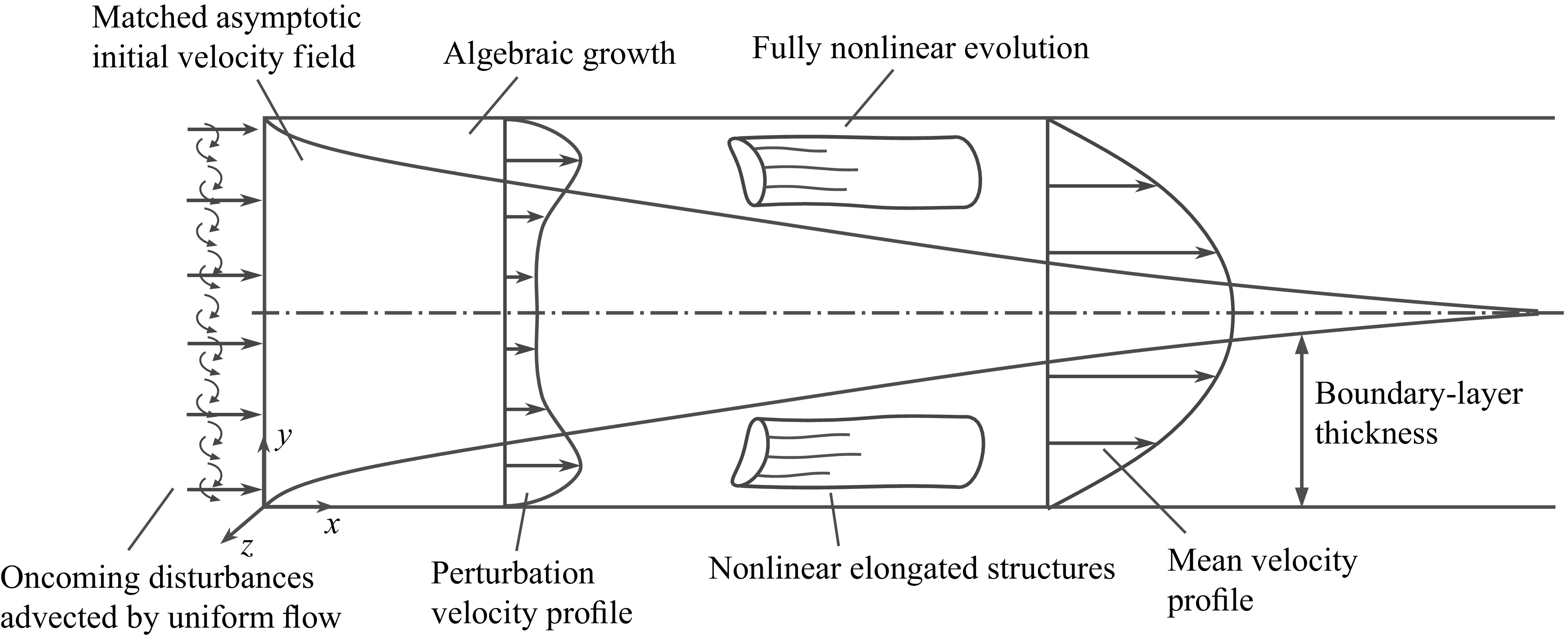


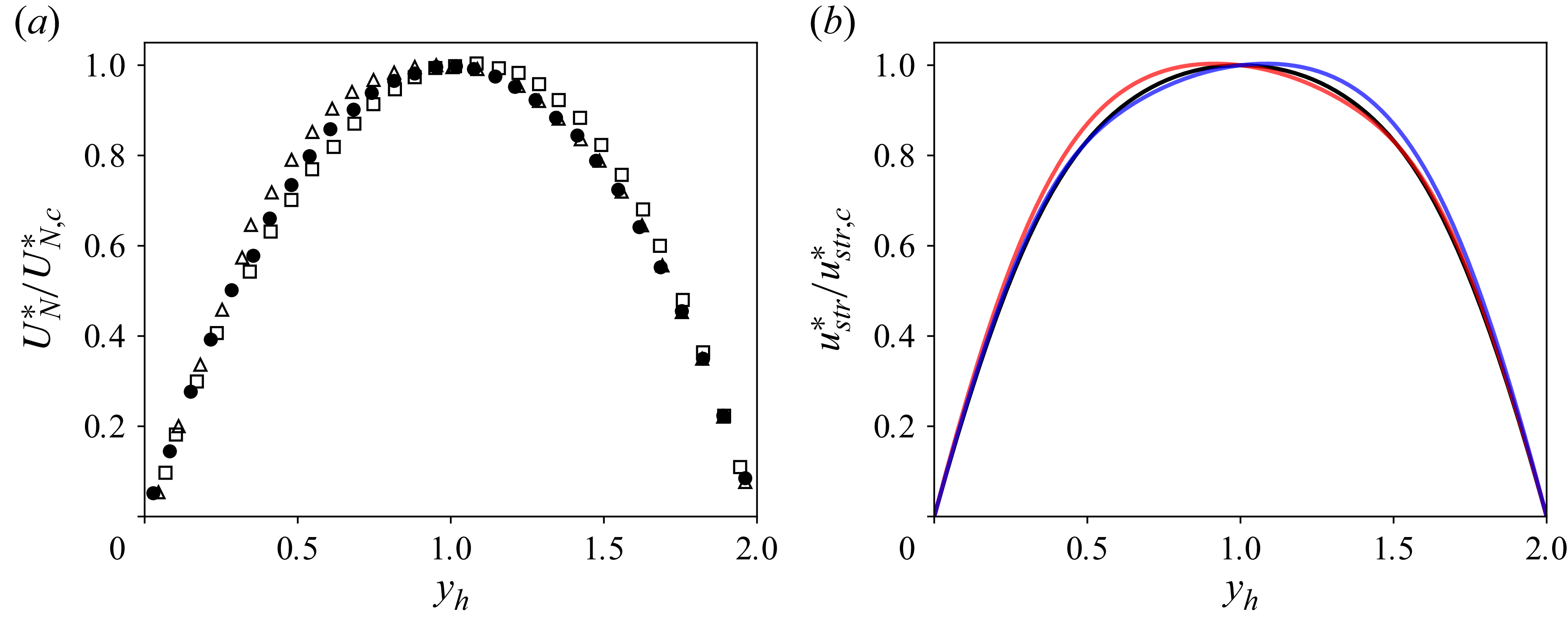


 Open access