


1. Introduction
As the total number of flights continues to increase each year, the noise produced by the aviation sector has become a well-established problem. The reduction of aircraft noise radiated to the ground during take off and landing is a priority for aviation authorities and is forcing aircraft manufacturers to invest in fundamental aeroacoustic research. Reduction in cruise noise is also crucial to improving in-cabin comfort for both passengers and crew. The key aircraft noise sources can be split into two parts: propulsive noise and airframe noise. The predominance of each source depends on the size of the aircraft and the stage of flight. During take off, jet noise continues to dominate in the sideline certification direction, whereas, during approach, the majority of the propulsive noise is generated by the fans. Airframe noise is most important during approach and is generally related to high-lift devices. Many studies have been performed on the topic of isolated jet mixing noise, neglecting any aerodynamic interaction between the jet exhaust plume and the airframe surfaces. Such jet installation effects are set to increase as under-wing-mounted engines continue to increase in size and move closer to the airframe surfaces, as predicted for ultra-high-bypass-ratio (UHBR) engines, for example.
The main focus of this work concerns the interaction between the jet exhaust flow and the wing. This jet–surface flow interaction results in the far-field acoustic propagation of otherwise evanescent hydrodynamic low-frequency sound. Various studies have demonstrated that this low-frequency amplification can be ascribed to the scattering of the jet's hydrodynamic field (Williams & Hall Reference Williams and Hall1970; Bushell Reference Bushell1975; Head & Fisher Reference Head and Fisher1976; Lyu, Dowling & Naqavi Reference Lyu, Dowling and Naqavi2017; Lyu & Dowling Reference Lyu and Dowling2019; Dawson et al. Reference Dawson, Lawrence, Self and Kingan2020). The fundamental physical understanding of this noise source has generally been represented using simplified geometries such as a flat plate instead of a wing. The aerodynamics of the interaction between the jet and the flat plate has been reported in several studies showing the presence of a Coand $\check{a}$ effect (see, for example, Di Marco, Mancinelli & Camussi Reference Di Marco, Mancinelli and Camussi2015; Proença, Lawrence & Self Reference Proença, Lawrence and Self2020b). The near-field pressure and far-field noise generated by a jet installed close to a semi-infinite plate has been analysed by Lawrence, Azarpeyvand & Self (Reference Lawrence, Azarpeyvand and Self2011) and Jordan et al. (Reference Jordan, Jaunet, Towne, Cavalieri, Colonius, Schmidt and Agarwal2017, Reference Jordan, Jaunet, Towne, Cavalieri, Colonius, Schmidt and Agarwal2018). The connection between jet installation noise and the flow-field features of the corresponding isolated jet has also been studied by Rego et al. (Reference Rego, Avallone, Ragni and Casalino2020) using lattice Boltzmann numerical simulations.
Jet installation effects have been studied in terms of the wall-pressure fluctuations induced on neighbouring surfaces. Preliminary studies for an incompressible flow adjacent to a plate were performed by Di Marco et al. (Reference Di Marco, Mancinelli and Camussi2015), who developed a wall-pressure spectral model, and by Mancinelli, Di Marco & Camussi (Reference Mancinelli, Di Marco and Camussi2017), who applied wavelet conditioning to the wall-pressure signal. Recently, Meloni et al. (Reference Meloni, Di Marco, Mancinelli and Camussi2019) investigated the wall-pressure field induced by a highly compressible subsonic jet on to an infinite flat plate, providing autospectra and cross-spectra scaling in terms of jet Mach number. Further studies have been performed for small-scale jet–wing–flap configurations, including the presence of a co-flow (Faranosov et al. Reference Faranosov, Bychkov, Kopiev, Soares and Cavalieri2019; Meloni et al. Reference Meloni, Mancinelli, Camussi and Huber2020b) and using a chevron nozzle (Mengle Reference Mengle2012).
The additional full-scale component considered here is a pylon geometry, which is used to attach each engine to the wing. Several publications considering the isolated jet mixing noise source (Bhat Reference Bhat2012; Viswanathan & Lee Reference Viswanathan and Lee2013) suggest that the pylon induces a flow asymmetry and, thus, an azimuthal variation in the far-field noise level. Regarding installed jet configurations, to date only numerical studies using a large-eddy simulation and Reynolds-averaged Navier–Stokes code have been reported by Semiletov et al. (Reference Semiletov, Karabasov, Lyubimov, Faranosov and Kopiev2013), Markesteijn & Karabasov (Reference Markesteijn and Karabasov2020), Massey et al. (Reference Massey, Elmiligui, Hunter, Thomas, Pao and Mengle2006). In addition to the pylon, Semiletov and colleagues also considered several flap deflection angles, showing good far-field acoustic spectral predictions. Finally, experimental investigations performed by Faranosov et al. (Reference Faranosov, Kopiev, Ostrikov and Kopiev2016), Czech, Thomas & Elkoby (Reference Czech, Thomas and Elkoby2012), showed that the pylon must be accounted for in order to correctly assess the noise emitted by close-coupled jet–wing configurations. To the best of the authors’ knowledge no study detailing the effect of the pylon blockage on both the near and far pressure fields of installed jets has been presented and this, therefore, is the main motivation for the present work.
In this paper, jet–surface interaction noise is investigated experimentally using two model-scale single-stream jets, an ‘annular’ axisymmetric jet, containing a centrebody, and a ‘pylon’ asymmetric jet, with a  $10\,\%$ flow-area blockage, installed beneath a NACA4415 aerofoil. A simple pylon-nozzle geometry, consisting of a symmetric aerodynamic profile, was used to investigate the effects of internal nozzle blockage on the noise emitted by an installed jet.
Single-component hot-wire velocity measurements as well as synchronous wall-pressure fluctuation and far-field acoustic measurements were recorded. The jet acoustic Mach number was varied between  $0.5 \leq M_{{j}} \leq 0.8$. The Doak Flight Jet Rig (FJR) was used to simulate the in-flight situation and the co-flow flight velocity was varied between $0 \leq M_{{f}} \leq 0.2$. Wall-pressure fluctuations were acquired using miniature wall-pressure transducers that were flush-mounted within the pressure surface of the wing in both the streamwise and spanwise directions close to the wing trailing edge. Far-field pressure data were acquired using a linear ‘flyover’ microphone array positioned on the unshielded side of the wing (i.e. at $\phi =0^{\circ }$) incorporating a polar observer angle range between $40^{\circ } \leq \theta \leq 130^{\circ }$. Multi-variate statistical analyses were performed to interpret the data. Comparisons between the installed and the isolated jet data were carried out for the static (i.e. at $M_{{f}}=0$) case.
The paper is organised as follows: in § 2, the experimental set-up is described in detail. Velocity-field results are reported in § 3. Sections 4 and 5 report the far-field noise and wall-pressure fluctuations, respectively. Final conclusions are provided in § 6.
2. Experimental set-up
Experiments were performed using the FJR in the Doak Laboratory at the University of Southampton. The Doak Laboratory is an anechoic chamber, fully anechoic above 400 Hz with dimensions approximately equal to 15 m long, 7 m wide and 5 m high. Two independent air supply systems allow in-flight simulations of single-stream jet flows. The primary ‘jet’ flow is supplied by a high-pressure compressor-reservoir system, capable of producing a maximum pressure of 20 bar. The secondary ‘flight’ flow is supplied by a 1.1 pressure-ratio fan. The flight nozzle-exhaust diameter is 300 mm and is capable of producing steady flows up to  $M_{{f}}=0.3$. Further information about the Doak Laboratory facility and the FJR can be found in Proença, Lawrence & Self (Reference Proença, Lawrence and Self2020a).
Measurements were performed using two 40 mm diameter jet nozzles connected to convergent pipework (with a 2.5 $^{\circ }$ internal convergence half-angle) over a length of 15D (where D is the nozzle exit diameter). The baseline annular nozzle contained a solid centrebody ‘bullet’ and thus produced an axisymmetric annular jet flow immediately downstream of the nozzle exit. The second pylon nozzle was identical to the baseline except for a blockage located at the top of the nozzle (i.e. adjacent to the wing surface), which reduced the nozzle-exit flow area by $10\,\%$. In both cases, the diameter of the bullet at the nozzle exit was equal to 24 mm and the bullet extended 35 mm downstream of the nozzle exit. For the annular jet, therefore, the effective jet diameter (based on mass flow rate) was equal to 32 mm. The pylon shape is defined as a circular sector at the nozzle exit blocking, as aforementioned, $10\,\%$ of the jet flow area. The internal nozzle blockage extended upstream of the nozzle exit plane, reducing in thickness with axial distance, with an aerodynamically faired leading edge. The external pylon-nozzle surfaces, downstream of the nozzle exit, were profiled using simple smooth splines starting from a point of tangency at the nozzle exit plane down to the end of the bullet centrebody and up to the pressure surface of the wing. The additional blockage created by the pylon reduced the effective nozzle exit diameter to 30.4 mm. The jet acoustic Mach number was varied from 0.5 to 0.8 in steps of 0.1 and the flight acoustic Mach number was varied from 0 to 0.2 in steps of 0.1.
A NACA4415 wing profile, with a 150 mm chord and a 600 mm span, was installed at  $H/D=0.6$, where $H$ is the vertical distance measured from the wing trailing edge to the jet centreline axis; $D$ is the nozzle exit internal diameter. A support structure was used to secure and position the wing relative to the jet. The wing was secured at an incidence angle of $4^{\circ }$ and the leading edge was positioned 40 mm upstream of the nozzle exit plane resulting in an axial trailing-edge location, relative to the nozzle exit, equal to $L/D=2.75$. A cartridge with a grid of holes 10 mm apart was manufactured to house miniature, flush-mountable wall-pressure transducers. The wall-pressure measurements were performed using a pair of Kulite LQ-062 transducers that have a sensing diameter equal to 1.6 mm. The transducer cartridge was secured on to the pressure side of the wing and any unused holes were covered with thin metal tape to avoid any vortex shedding effects and cavity resonances. Measurements were performed in the streamwise direction between $x/D=1.22$ and $x/D=2.47$ downstream of the nozzle exit. The spanwise position of the wall-pressure transducers was varied between $y/D=0$ and $y/D=1$, keeping the streamwise position fixed at
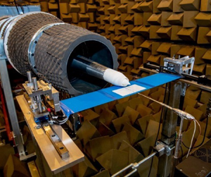
  $x/D=2.47$. A graphical representation of the Kulite positions is shown in figure 1. The frame of reference for all results is fixed at the nozzle exit, as depicted in figure 1(a). A photograph of the experimental set-up is shown in figure 1(b). The configuration selected and the wing geometrical parameters adopted derive from an extensive study carried out under EU funded projects dedicated to the assessment of installation effects of UHBR engines (e.g. JERONIMO, ARTEM).
(a) Schematic of the experimental set-up with the microphone locations, and (b) photograph of the installed jet aerodynamic measurement set-up using the FJR, in the Doak Laboratory.

The far-field acoustic data were acquired synchronously with the wall-pressure data. The far-field flyover array, consisting of ten 1/4” B $\&$K 4939 microphones, was positioned at a radial distance of 2.14 m from the jet axis and incorporated polar angles between $40^{\circ } \leq \theta \leq 130^{\circ }$. The data were acquired for 10 s at a sampling frequency of 200 kHz. The wall-pressure transducer signals were acquired using a Kulite KSC2 signal conditioner unit with a 5 V excitation voltage and a 100 kHz low-pass filter.
Separate single-point, single-component turbulent velocity measurements were performed using a constant temperature anemometry system in the  $x$–
$x$– $z$ plane between $1 \leq x/D \leq 3$ and between $-2 \leq z/D \leq 2$. A Dantec 5511 hot-wire probe was positioned with an ISEL three-axis traverse system. The sampling frequency for the velocity measurements was set at 50 kHz.
3. Velocity-field results
Velocity profiles measured in the radial direction at different axial positions provide an overall estimation of the influence of the bullet and the pylon on the jet flow field, as reported in figure 2. Two different axial jet locations pertinent to the region of jet–wing interaction are presented under static and in-flight ambient flow conditions. Owing to the close-coupled jet–pylon–wing location investigated in this work, the jet flow impacts the wing at  $x/D=1.2$ and $x/D=1.1$ for the annular and pylon jets, respectively. This interaction provides a further azimuthal asymmetry in the velocity profile between negative and positive $z/D$, see Appendix for further details.
Normalised mean axial velocity installed jet radial profiles at  $M_{j}=0.6$: (a) $x/D=1$, $M_{f}=0$; (b) $x/D=3$, $M_{f}=0$; (c) $x/D=1$, $M_{f}=0.2$; (d) $x/D=3$, $M_{f}=0.2$.

In both cases, the main effects provided by the bullet and the pylon are observed very close to the nozzle, i.e. at  $x/D=1$, see figures 2(a) and 2(c). As expected, the bullet is seen to block the jet flow close to the jet centreline. No significant effects, however, were observed beyond the jet lip-line. For the pylon case, an additional mean axial-velocity decrease is seen in the positive $z/D$ direction owing to the internal pylon blockage. The velocity reduction at positive z/D in the pylon case can probably be ascribed to the wake created immediately behind the pylon. The pylon presence indeed alters the azimuthal symmetry of the jet, producing an oval jet shape (see Appendix). In figure 2(b), both the bullet and pylon effects are seen to reduce with increasing axial distance. In all cases, the presence of the flight flow is seen to have a weak influence on the magnitude of the normalised mean velocity. The sharp drop in velocity observed at positive $z/D$, in figures 2(b) and 2(d), is related to the position of the hot-wire probe, which is one millimetre beyond the wing trailing edge, in a low-velocity flow region.
Similar results are obtained for the turbulence intensity (TI), evaluated according to the following definition:
 \begin{equation} {TI}=\frac{\sigma_{u}}{U_{{j}}}, \end{equation}
where  $\sigma _{u}$ is the velocity standard deviation and $U_j$ is the nominal jet exit velocity, defined by the ratio between the upstream plenum pressure and the ambient chamber pressure. Figure 3 shows the TI radial profiles at two axial locations ( $x/D=1$ and $x/D=3$) under static and in-flight ambient flow conditions. Owing to the close-coupled jet–pylon–wing location investigated in this work, the jet flow strongly interacts with the wing surface close to the trailing edge. This interaction generates a grazing flow and a further asymmetry in the velocity profile between negative and positive $z/D$. Further details can be found in the Appendix. A slight difference is detected between the pylon and the annular configuration for both the static and in-flight cases.
Normalised mean TI installed jet radial profiles at  $M_{j}=0.6$: (a) $x/D=1$, $M_{f}=0$; (b) $x/D=3$, $M_{f}=0$; (c) $x/D=1$, $M_{f}=0.2$; (d) $x/D=3$, $M_{f}=0.2$.

For the mean velocity profiles, an asymmetry occurs in the position of the maximum TI for the static pylon case at  $x/D=1$, see figure 3(a). Note that the TI peak on the lower free side of the jet (i.e at negative $z/D$) is larger than the peak on the upper pylon side of the jet (i.e. at positive $z/D$). This effect is due to the fact that the usual mixing in the upper jet shear layer is delayed by the presence of the pylon. It is interesting to note, however, that, for the in-flight case, the asymmetry is reversed; see figure 3(c) where the larger peak is seen at positive $z/D$. The authors suggest that this behaviour is caused by the presence of a wake formed behind the external part of the pylon between the nozzle and wing. In the static case, the pylon device slightly increases the TI downstream of the wing trailing edge. For the in-flight cases, however, the TI difference between the pylon- and annular-nozzle flows is up to 10 % greater. For the in-flight case, it is unclear exactly what the impact of the wake field created by the flight flow around the external pylon blockage is.
This effect is still evident, although significantly reduced farther downstream at  ${x/D=3}$ (see figures 3(b) and 3(d)), as the wake disappears and the jet recovers a more homogeneous mixing profile. Furthermore, at this location, the flight-stream flow does not appear to affect the shape of the TI profiles significantly.
In summary, this analysis shows that the pylon modifies the mean flow field of the jet observed upstream of the aerofoil trailing edge. The next sections assess whether such asymmetric mean flow effects significantly alter the far-field acoustic pressure and the wall-pressure fluctuations.
4. Far-field noise results
4.1. Isolated versus installed pylon-jet effects
To ascertain the influence of the wing and pylon effects separately, static jet measurements without the wing (denoted as ‘isolated’) were performed at  $M_{{j}}=0.6$ and $M_{{j}}=0.8$. Examples of the spectral analysis in terms of sound pressure level (SPL), defined in the following equation, are reported, for different polar angles, in figure 4:
 \begin{equation} SPL=10 \log_{10} \left(\frac{ {PSD} {\rm \Delta} f_{{ref}}}{P_{{ref}}^{2}}\right),\end{equation}
where PSD denotes the power spectral density evaluated using Welch's method,  ${\rm \Delta} f_{{ref}}$ is the frequency bandwidth and $P_{{ref}}$ is the reference pressure in air (equal to $20\ \mathrm {\mu }$Pa). Free-field microphone incidence and atmospheric attenuation corrections are also applied to the data. The Welch method has been applied using a window size of 2048 samples with the overlap fixed at $50\,\%$. The present data have been corrected to take into account the atmospheric attenuation. The correction, as described in Bass et al. (Reference Bass, Sutherland, Zuckerwar, Blackstock and Hester1995) and Kinsler et al. (Reference Kinsler, Frey, Coppens and Sanders1999), is a function of the relative humidity, ambient temperature, ambient pressure and the distance between each microphone and the nozzle exit. Finally, the data were corrected to a $1$ m lossless distance using the spherical-wave propagation assumption. Strictly speaking, a further 0.5 dB correction based on nozzle-exit flow area should be added to the isolated pylon-jet far-field noise data when looking to compare the two nozzles on a constant thrust basis. In this paper, however, the authors have omitted this correction for simplicity owing to the open question surrounding the correct method to scale the far-field installed jet data.
Far-field SPL spectral comparison between the static isolated (solid lines) and installed (dashed lines) jets at different polar angles and jet Mach numbers: (a)  $\theta =40^{\circ }$ and $M_{{j}}=0.6$; (b) $\theta =40^{\circ }$ and $M_{{j}}=0.8$; (c) $\theta =90^{\circ }$ and $M_{{j}}=0.6$; (d) $\theta =90^{\circ }$ and $M_{{j}}=0.8$; (e) $\theta =130^{\circ }$ and $M_{{j}}=0.6$; (f) $\theta =130^{\circ }$ and $M_{{j}}=0.8$.

In figure 4, an amplification of the low-frequency noise ascribed to the scattering of the jet hydrodynamic field is clearly observed. As expected, the relative amplification, with respect to the isolated jet noise, reduces with increasing jet velocity at all polar angles. The effect of the presence of the pylon on the far-field noise is seen to be negligible in the isolated jet case. However, even if one were to include the isolated jet flow-area correction, the pylon device is observed to provide a maximum noise difference of 2.5 dB below the annular jet at  $M_{{j}}=0.6$ (including the flow-area correction) at this single azimuthal observer angle. This maximum noise difference reduces to 1 dB at $M_{{j}}=0.8$. Specifically, this noise reduction is observed in the low-frequency region and depends on both polar angle and jet Mach number. The authors suggest that the noise difference observed between the annular and pylon jets is due to the degree to which the pylon wake flow interacts with the wing surface. Indeed, the velocity profiles shown in figures 2 and 3 add evidence to the claim that a pylon wake flow exists. The fact that the increase in jet Mach number causes a reduction in the noise difference between the two nozzles is further evidence to back up this hypothesis, because one would expect the velocity deficit generated by a wake to have a greater impact on the local mixing rate for a slower compared with a faster jet flow. This hypothesis is further investigated in the next section using the wall-pressure data.
The far-field analysis is now presented in a more general way, considering all polar angles, using the overall sound pressure level (OASPL), defined as follows:
 \begin{equation} {OASPL}=10 \log_{10} \left(\frac{p^{\prime 2}}{P_{{ref}}^{2}}\right).\end{equation}
Because the lowest-frequency acoustic energy, below the anechoic limit of the chamber (i.e.  $f < 400$ Hz), contains unwanted reflections and the highest-frequency energy contains non-physical background noise, $p'^{2}$ is computed via integration of the PSD over a frequency range:
 \begin{equation} p'^{2}= \int_{f_1}^{f_2} {PSD}(f)\, {\textrm{d}}f, \end{equation}
where  $f_1$ is 400 Hz and $f_2$ is 20 kHz. The OASPL analysis is reported in figure 5. The jet–surface interaction source, as expected, creates a significant increase in noise for both nozzle configurations, mainly at large polar angles in the forward arc. As with the spectral analysis, the pylon is seen to have a negligible effect on the isolated jet mixing noise emitted to the far field. This is consistent for all polar angles studied. For the installed jet configuration, the pylon nozzle is seen to produce less noise in the far field compared with the annular nozzle. This is true for most of the polar angles and a 1–3 dB difference is observed at $M_{{j}}=0.6$. At $M_{{j}} = 0.8$, as expected, in the rear polar arc the noise emitted is dominated by jet mixing noise.
Far-field OASPL comparison between the static isolated (solid lines) and installed (dashed lines) jets: (a)  $M_{{j}}=0.6$; (b) $M_{{j}}=0.8$.

4.2. Installed jet static versus flight analysis
The installed far-field noise from the static versus the in-flight ambient flow situations were first investigated in the frequency domain, again using the SPL quantity defined in (4.1). Far-field jet spectra at  $M_j=0.8$ are presented in figure 6 at several polar angles at $M_{{f}}=0.0, 0.1, 0.2$). The installed flight background noise is also shown in each panel as green (annular) and black (pylon) lines. The flight background noise, defined as the noise from just the flight-stream flow over the jet–wing model, was produced by matching the jet to the flight velocity.
Far-field SPL spectral comparison between the static installed (solid lines) and in-flight installed (dashed lines) jets at  $M_{{j}}=0.8$ for different polar angles at $M_{{f}}=0.1$ (a,c,e) and $M_{{f}}=0.2$ (b,d,f): (a,b) $\theta =40^{\circ }$; (c,d) $\theta =90^{\circ }$; (e,f) $\theta =130^{\circ }$.

As expected, the forward-flight flow leads to an overall decrease in the magnitude of the spectral energy, particularly at  $M_{{f}}=0.2$. The degree of noise reduction is strongly dependent on polar angle and frequency. In figures 6(a,b), a constant noise reduction of approximately 4–6 dB is observed at the low polar angles. At higher polar angles, the in-flight noise reduction is not so prominent, especially at high frequencies.
Interestingly, the flight background noise is seen to dominate the lowest frequencies (i.e. below  $800$ Hz) of the jet–surface interaction noise at $M_{{f}}>0.1$.
For both the static and in-flight cases, the effect of the pylon is negligible at the low-observer polar angles. At high polar angles, the noise reduction provided by the pylon is observed to be strongly frequency-dependent and is clearly the result of a change to the hydrodynamic low-frequency jet–surface interaction source field. In order to quantify this difference, a  ${\rm \Delta} SPL$ quantity is defined as follows:
 \begin{equation} {\rm \Delta} {SPL}(f)={SPL}_{annular}(f) - {SPL}_{pylon}(f). \end{equation}
 This quantity is reported in figure 7 for three polar angles. For display clarity, the narrow-band spectral data have been converted to one-third octave bands. Considering figure 7(a,b), it is clear that the effect of the pylon in both the static and in-flight cases is less than 1 dB at all frequencies at  $\theta =40^{\circ }$. The increase in flight velocity appears to increase the noise difference between the two configurations at high frequency and at all polar angles (see figure 7b,d,f).
Far-field  ${\rm \Delta} SPL$ between the annular and pylon installed jets at $M_{{f}}=0.1$ (a,c,e) and $M_{{f}}=0.2$ (b,d,f): (a,b) $\theta =40^{\circ }$; (c,d) $\theta =90^{\circ }$; (e,f) $\theta =130^{\circ }$.

As before, an overview of the in-flight effects is performed using the OASPL quantity, defined in (4.2). The data presented in figure 8(a,b) confirm that the pylon principally effects the noise propagated to the high polar angles. This trend is even clearer to see when one looks at the difference between the annular- and pylon-nozzle OASPL values, simply defined as follows:
 \begin{equation} {\rm \Delta} {OASPL}={OASPL}_{annular} - {OASPL}_{pylon},\end{equation}
As displayed in figures 8(c,d), the  ${\rm \Delta} OASPL$ between the annular and pylon jets appears to increase with increasing polar angle and becomes even stronger in flight. More specifically, the co-flow appears to have a significant effect at polar angles between $60^{\circ } \leq \theta \leq 100^{\circ }$.
Far-field OASPL (a,b) and  ${\rm \Delta} OASPL$ (c,d) static versus in-flight comparison between the installed annular and pylon jets at $M_j=0.8$: (a,c) $M_{{f}}=0.1$, (b,d) $M_{{f}}=0.2$.

5. Wall-pressure field
5.1. Streamwise analysis
The wall-pressure data were first evaluated in the frequency domain, again using the SPL quantity, defined in (4.1). In figure 9, the streamwise wall-pressure autospectra at  ${M_{{j}}=0.8}$ are reported at the three flight velocities. Figure 9(a,b) show that at $x/D=1.22$ the magnitude of the spectra are significantly reduced when the pylon is present. This is true for both the static and in-flight situations. In addition to the SPL reduction, the pylon also appears to modify the spectral shape at frequencies above the peak.
Static versus in-flight comparison between the installed annular- and pylon-jet wall-pressure SPL spectra at  $M_{{f}}=0.1$ (a,c,e) and $M_{{f}}=0.2$ (b,d,f) and at $M_{{j}}=0.8$ and $y/D=0$: (a,b) $x/D=1.22$; (c,d) $x/D=1.72$; (e,f) $x/D=2.47$.

Figure 9(a,b) show that the spectral energy for the pylon jet decays as  $f^{-6.67}$ between $f\approx 2.5$ kHz and $f\approx 8$ kHz. According to Arndt, Long & Glauser (Reference Arndt, Long and Glauser1997), this decay law is typical of the linear, irrotational hydrodynamic region of the flow, a behaviour observed in the near field of free jets where the pressure field is dominated by Kelvin–Helmholtz instability waves (see, among many, George, Beuther & Arndt Reference George, Beuther and Arndt1984; Tinney & Jordan Reference Tinney and Jordan2008). At higher frequencies, an $f^{-2}$ slope, which describes the linear acoustic region (Arndt et al. Reference Arndt, Long and Glauser1997), is visible for the pylon-jet case. The hydrodynamic field generated by the annular jet contains significantly more high-frequency energy than the pylon jet. The authors suggest that the difference in shape is assumed to be due to the presence of the wake field generated behind the pylon that serves to restrict the development (and hence the magnitude) of the hydrodynamic field in the jet shear layer local to the pylon. This reduction of the jet's hydrodynamic field strength essentially reveals its acoustic field at a much lower frequency compared with the unrestricted annular-jet case. The final observation to make from figure 9 is that the co-flow does not appear to influence the spectral shape of the pylon-jet wall-pressure field significantly. The co-flow does, however, appear to affect the spectral shape of the annular jet at frequencies above the peak. The authors suggest that this additional high-frequency energy, observed only in the flight case, is probably owing to the fact that the Kelvin–Helmholtz instability in the jet shear layer next to the aerofoil surface is unrestricted in the annular-jet case. To confirm this hypothesis, further analyses are needed. This would enable a greater degree of hydrodynamic-field development compared with the blocked pylon-jet case at locations close to the nozzle/pylon. Furthermore, the jet stretching effect owing to the presence of the co-flow would naturally increase the upper-frequency range of the hydrodynamic field observed at a given axial location compared with the static jet case. This can be ascribed to the reduction of the jet shear layer width at a given axial location, which inherently will result in higher-frequency noise generation. Further in-flight installed jet aerodynamic investigation is required, however, to confirm this hypothesis. Finally, as one moves farther downstream closer to the aerofoil trailing edge, the effect of the pylon is seen to reduce at all frequencies, see figure 9(e,f). The co-flow also appears to have a reduced influence on both the shape and magnitude of the wall-pressure spectrum here. Clearly, both the pylon and co-flow only appear to influence the development of the jet's hydrodynamic field locally downstream of the pylon trailing edge.
For increasing  $x/D$, see figure 9(c,d), the difference between the annular and pylon spectra decreases until the farthest downstream position close to the wing trailing edge, see figure 9(e,f), where the wall-pressure spectra of the annular and pylon jets collapse both for the static and in-flight situations. Here, the spectral decay law is close to $f^{-7/3}$, which is typical of fully developed turbulence (George et al. Reference George, Beuther and Arndt1984) and has previously been observed in wall-pressure fluctuation data from fully developed grazing jet flows (Meloni et al. Reference Meloni, Di Marco, Mancinelli and Camussi2019, Reference Meloni, Mancinelli, Camussi and Huber2020b).
The in-flight wall-pressure spectra are also reported in figure 9 together with the flight background noise, shown as dashed lines. More so than for the acoustic far-field pressure, the lowest frequencies in the near-field spectra closest to the pylon appear to be dominated by the background noise. This result may have important implications for the positioning of future airframe surface-mounted sensors on full-scale aircraft when there is a requirement to record validation data for industrial noise-prediction methods. At higher flight velocities (more representative of the approach certification location, for example), the signal-to-noise ratio will probably reduce even further and risk masking significant portions of the frequency range pertinent to the jet–surface interaction noise source.
An overall picture of the low-order statistical properties of the streamwise wall-pressure fluctuations for both the static and in-flight cases is presented in figure 10. The streamwise evolution of the  ${OASPL}$ along the pressure side of the wing is illustrated in figure 10(a,b) for the two jets at the two flight velocities. Consistently with previous studies on a jet–wing configuration (e.g. Meloni et al. Reference Meloni, Mancinelli, Camussi and Huber2020b), the trends of these low-order statistical quantities are found to be slightly dependent on flight velocity. The increase in ${OASPL}$ with increasing streamwise distance is ascribed to the increased proximity between the jet and the surface as the jet develops and spreads towards the aerofoil.
Static versus in-flight comparison of the streamwise evolution wall-pressure fluctuations for the installed annular and pylon jets at  $M_{{f}}=0.1$ (a,c) and $M_{{f}}=0.2$ (b,d) at $y/D=0$: (a,b) OASPL; (c,d) ${\rm \Delta} OASPL$.

As seen with the SPL analysis, figure 10(a,b) shows a reduction in the magnitude of the wall-pressure fluctuations for the pylon jet compared with the annular jet under both static and in-flight ambient flow conditions. This effect can be ascribed to the blockage created by the pylon close to the nozzle exhaust, as shown previously in figure 2. A kink in the  ${OASPL}$ trend is also detected for the annular jet both statically and in flight at $x/D\approx 2$. The kink also appears to be amplified at $M_f=0.2$, see figure 10(b). The authors suggest that this artefact results from a delay in high-frequency fluctuation generation compared with the annular case. While this streamwise surface location roughly corresponds to the position at which the jet's rotational hydrodynamic field actually impacts the aerofoil, further installed aerodynamic and wall-pressure data with a finer spatial resolution are required to confirm this hypothesis. Interestingly, this kink does not exist for the pylon-jet case. Clearly, more information about the development of both the rotational and irrotational hydrodynamic fields of these two installed jet flows is required in order to fully explain this result.
As before, the  ${OASPL}$ variation is determined using the ${\rm \Delta} {OASPL}$ quantity. The ${\rm \Delta} {OASPL}$ data, see figure 10(c), are seen to decrease with increasing axial distance. As before, one can explain this by the local flow blockage effect behind the pylon, which serves to restrict the development of the jet's hydrodynamic field in the shear layer adjacent to the aerofoil surface. Additionally, the ${\rm \Delta} {OASPL}$ is seen to increase with increasing flight velocity, which is consistent with the SPL trend discussed previously.
Analysis of the higher-order statistical moments provides further physical insight into the behaviour of the flow along the wing surface. The skewness and kurtosis are defined as follows:
 \begin{gather} s=\frac{E(p-\mu)^{3}}{\sigma_{p}^{3}}, \end{gather}
 \begin{gather}k=\frac{E(p-\mu)^{4}}{\sigma_{p}^{4}}, \end{gather}
where  $\mu$ is the mean of $p$ and E() is the expected value. According to theory, if a signal follows a Gaussian distribution, the skewness will tend to zero and the kurtosis to three. Thus, they are useful in identifying non-Gaussian features (Meloni et al. Reference Meloni, Lawrence, Proença, Self and Camussi2020a). The skewness factor, reported in figure 11(a,b) is close to zero at small $x/D$ and tends to increase revealing the prevalence of positive (i.e. larger than the mean) rather than negative events. This is due to the prominence of positive pressure events induced by the jet over the wing, as reported by Meloni et al. (Reference Meloni, Lawrence, Proença, Self and Camussi2020a). The effect of the pylon does not appear to be significant even though a spatial shift of the skewness peak is observed as an effect of the interaction between the wake generated by the pylon and the wing surface. It is also evident that, as previously observed, the influence of flight velocity is weak, particularly for the pylon-jet case. The effect of flight velocity can be seen in the steeper increase in skewness with increasing $x/D$, particularly for the annular-jet case. The authors believe this to be caused by the earlier impact of the flight-stream turbulent structures compared with the blocked pylon-jet case, which induce positive intermittent pressure events on the pressure side of the wing. This is not particularly evident in the pylon case because the pylon restricts the development of turbulent structures within the flight flow. As a matter of fact, if we observe the skewness trends for the flight background data, the skewness is close to zero for the pylon nozzle and negative for the annular nozzle. A slight negative skewness means that the development of the turbulence is transitional and, therefore, can be ascribed to the flight turbulent structures interacting with the pressure side of the wing.
Static versus in-flight comparison of the streamwise evolution of the higher-order statistical wall-pressure quantities for the installed annular and pylon jets at  $M_{{f}}=0.1$ (a,c) and $M_{{f}}=0.2$ (b,d) at $y/D=0$: (a,b) skewness; (c,d) kurtosis.

The kurtosis values are reported in figure 11(c,d). The streamwise evolution of the kurtosis is weakly affected by both the presence of the pylon and the jet Mach number. The kurtosis tends to increase for increasing  $x/D$ owing to the development of the wall jet along the wing. For the in-flight situation, the kurtosis values are higher than three for all cases. This means that the detected pressure events have a probability density function larger than a normal distribution, which indicates that highly intermittent pressure events exist, from the coherent structures within the co-flow.
Two-point statistics were used to evaluate the streamwise phase velocity,  $U_{p}$, defined as the ratio between the transducer axial-separation distance $\xi$ and the time lag at which the cross-correlation coefficient is a maximum. This parameter is important when analysing the dynamics of the flow over the pressure surface of the wing, see Meloni et al. (Reference Meloni, Di Marco, Mancinelli and Camussi2019) and Meloni et al. (Reference Meloni, Mancinelli, Camussi and Huber2020b). The streamwise phase speed of the pressure field that convects along the plate surface is reported in figure 12, for the two nozzles and three flight conditions.
Static versus in-flight comparison of the streamwise evolution of the wall-pressure fluctuation phase speed of the pylon versus the annular jet at  $y/D=0$ and $M_{{j}}=0.8$: (a) $M_f=0.1$; (b) $M_f=0.2$.

Close to the pylon (i.e. at  $x/D < 1.75$), no significant variation in the phase speed is observed. Farther downstream, however, the annular-jet phase speed increases and deviates from the pylon jet which decreases. This difference in phase speed must be a result of the wake flow (i.e. the velocity deficit) generated behind the pylon; however, further investigation is required to confirm the specifics of the pressure generation from such a complex velocity field. Comparing the static with the in-flight case, see figure 12(a,b), the co-flow appears to slightly increase the magnitude of the phase speed only for the annular jet. Presumably this is because the co-flow is unimpeded compared with the pylon case. Interestingly, a phase speed analysis of the flight background wall-pressure field is also reported in figure 12 for both flight velocities. For the annular nozzle, the trend appears to be similar to that observed with the jet flow, although with slightly higher values. The opposite trend is observed for the pylon nozzle. The authors believe that this increase is due to a local acceleration of the flight flow through the vertical gap between the nozzle and aerofoil surface. Again, further data are required to evidence this hypothesis.
5.2. Spanwise trailing-edge analysis
The wall-pressure SPL spectra in the spanwise direction are shown in figure 13. The influence of the pylon and co-flow velocity, as expected, depends strongly on the spanwise position owing to the relative strength of the jet versus the flight hydrodynamic pressure fields. If one first considers the spectra at  $y/D=0.25$, the effect of the pylon-jet flow on the spectral shape of the wall-pressure field is mostly observed at high frequency. For the static case (solid lines) at $y/D=1$, the effect the pylon has on the wall-pressure spectra is not appreciable. At $y/D=1$, the typical spectral decay laws expected for acoustic and hydrodynamic pressure fluctuations generated by a shear layer are observed for both nozzles. At this spanwise location, the pylon presence reduces the energy content over the frequency range pertinent to hydrodynamic fluctuations, see Arndt et al. (Reference Arndt, Long and Glauser1997). The acoustic fluctuations are observed at a slightly lower frequency in the pylon jet compared with the annular jet.
Static versus in-flight comparison of the spanwise evolution of wall SPL for the installed annular and pylon jets at  $M_{{f}}=0.1$ (a,c) and $M_{{f}}=0.2$ (b,d) at $x/D=2.47$ and $M_{{j}}=0.8$: (a,b) $y/D=0.25$; (c,d) $y/D=1$.

The effect of co-flow depends on the spanwise position and, as expected, the more significant effect is seen at  $y/D=1$, where the strength of the jet's hydrodynamic field is less. In this location, the strength of the jet's hydrodynamic field is comparable with that generated by the co-flow. The co-flow results in a reduction in the magnitude of the spectral energy content at all frequencies and a similar effect is observed for both nozzles. At $y/D=0.25$, however, the co-flow is seen to reduce only the lower-frequency spectral energy.
Finally, when considering the flight background spectra, the pylon jet is seen to produce a higher amplitude fluctuation compared with the annular jet. In addition, at large  $y/D$, it is clear to see the relative magnitudes of the hydrodynamic pressure fields generated by the jet and the flight flows.
The OASPL (see (4.2)) and  ${\rm \Delta} OASPL$ (see (4.5)) results are presented in figure 14. First, considering the static case, as expected, the wall-pressure OASPL decreases with increasing spanwise distance owing to the reduction of the axial-jet velocity component as the flow mixes and spreads radially. In the annular-jet case, a kink is observed at $y/D=0.5$ compared with the linear decay found in the pylon-jet case. This can be seen even more clearly in the ${\rm \Delta} OASPL$ data in figure 14(c,d). Similarly as found in the streamwise wall-pressure analysis, the authors suggest that this point relates to an ‘impact’ point at which the rotational hydrodynamic jet field begins to scrub the aerofoil surface. In this scenario, before a fully developed wall jet is set-up, the highly intermittent pressure events produced at the edge of the jet shear layer would dominate the fluctuations seen on the surface. As seen with the SPL analysis, the co-flow reduces the magnitude of the wall-pressure fluctuations, particularly at large $y/D$, and this effect increases with increasing flight velocity. In both the static and in-flight situations, the pylon presence is seen to reduce the wall-pressure OASPL in the spanwise direction. This result is consistent with the discussion provided for the streamwise wall-pressure analysis, where the authors suggested that the pylon blockage restricts the growth of the Kelvin–Helmholtz instability in the shear layer adjacent to the aerofoil surface and, thus, decreases the magnitude of the jet's hydrodynamic field locally downstream of the pylon. Two-point velocity correlation data together with an instability analysis describing the wake field behind the pylon would provide the evidence required to corroborate this hypothesis.
Static versus in-flight comparison of the spanwise evolution of wall-pressure fluctuations for the installed annular and pylon jets at  $M_{{f}}=0.1$ (a,c) and $M_{{f}}=0.2$ (b,d) at $x/D=2.47$ and $M_{{j}}=0.8$: (a,b) OASPL; (c,d) ${\rm \Delta} OASPL$.

6. Conclusions
An experimental investigation detailing the effect a pylon blockage has on the generation of the near and far pressure fields of a model-scale, single-stream installed pylon-jet configuration has been presented. The study included far-field noise and wall-pressure fluctuation analyses, the consideration of both static and in-flight ambient flow conditions, as well as a single-velocity-component hot-wire aerodynamic survey.
The experimental set-up consisted of two nozzles, one with a bullet fixed on the jet centreline and the other with an additional pylon connected to the wing. The nozzles were installed adjacent to a NACA4415 profile aerofoil wing at a single nozzle–wing location. The wing and nozzles were all three-dimensionally printed. A removable transducer cartridge was embedded within the pressure surface of the wing such that a pair of miniature wall-pressure sensors could be flush-mounted in either a streamwise or spanwise configuration on the wing surface.
An aerodynamic survey was carried out using a single hot-wire anemometer probe to determine the behaviour of the two flows. Regarding the mean axial-velocity flow field, an azimuthally asymmetric effect was observed for the pylon jet in the positive  $z$-direction (i.e. towards the pylon). In fact, mean flow-field modifications were observed both owing to the bullet and the presence of the pylon. These flow effects were seen to reduce with increasing axial distance. The flight co-flow was seen to have a weak influence on the normalised mean velocity amplitude. The TI data show a slight difference between the pylon and the annular configuration in the static case. Specifically, a higher TI was detected in the annular-jet case close to the nozzle at positive $z/D$. This was ascribed to the internal nozzle blockage provided by the pylon jet, which served to restrict the mixing of the jet immediately behind the pylon. This same trend was also observed farther downstream, although to a lesser degree. The presence of the co-flow, however, reversed this effect as a higher TI was observed for the pylon jet at positive $z/D$. The authors ascribed this to the development of a pylon wake field generated by the flight flow around the external part of the pylon.
The far-field installed jet noise was investigated using a linear flyover microphone array. Comparisons between the installed and isolated jets, firstly under static ambient flow conditions, showed that, as expected, the presence of the surface introduces a significant low-frequency noise increase that peaks in the forward polar arc. The presence of the pylon did not cause a discernible effect to the mixing noise for the isolated jet case, but it did cause a reduction, in the far-field noise for the installed configuration, even when one includes a standard nozzle flow-area correction. This installed pylon-jet effect was mainly at frequencies lower than  $f = 5$ kHz and at high polar angles. Finally, as expected, the jet mixing noise was seen to mask the low-frequency jet–surface interaction noise for both nozzles at high jet Mach numbers (i.e. $M_j=0.8$) and low polar angles.
The far-field analysis was extended by investigating the noise emitted by the two nozzles in-flight while fixing the jet Mach number at  $M_j=0.8$. As expected, the co-flow was seen to reduce the magnitude of the acoustic energy produced by both nozzles at all frequencies as flight Mach number increased. At the highest flight velocity, the noise difference between the two configurations was observed to increase significantly at high frequencies. Furthermore, the flight background noise, evaluated by matching the jet and flight velocities, was seen to dominate at very low frequency.
The investigation continued with the near-field analysis performed in terms of wall-pressure fluctuations, using transducers flush-mounted on the pressure surface of the wing. The wall-pressure field was seen to be strongly influenced by the two different nozzles, especially at streamwise locations close to the pylon trailing edge. The authors suggest this to be a consequence of the wake field generated behind the pylon that serves to disrupt the development of the jet's hydrodynamic field local to the pylon. The irrotational hydrodynamic and acoustic fields were detected in the spectral decay of the wall-pressure fluctuations for the pylon nozzle close to the pylon trailing edge. At this location, the pylon presence was also observed to provide a significant reduction in the magnitude of the wall-pressure fluctuations. At locations farther downstream, closer to the wing trailing edge, the pylon presence was seen to be less influential on the magnitude and shape of the wall-pressure spectra. For the in-flight analysis, the presence of the co-flow was seen to modify the spectral shape of the wall-pressure field from both nozzles at small values of  $x/D$ by a reduction in the magnitude of the mid-frequency hydrodynamic peak. Furthermore, for the annular-jet case, an increase in wall-pressure fluctuation magnitude was seen at high frequencies. Any flight effects at large streamwise locations were found to be negligible.
Finally, the wall-pressure flight background noise showed a slightly higher magnitude for the pylon nozzle than the annular nozzle at low frequencies and close to the nozzle. This difference was observed at all frequencies and increased with flight velocity and at farther downstream streamwise positions.
Analysis of the two-point wall-pressure fluctuation statistics highlighted a variation in the phase speed with increasing flight velocity. An increase in the phase speed was observed close to the nozzle exit only for the in-flight annular jet. The authors believe this to be due to a local acceleration of flight co-flow through the gap between the nozzle and wing. Further experimental or numerical investigation is required, however, to evidence this flow behaviour. No significant flight effect was observed for the pylon-nozzle case.
The statistical wall-pressure analysis was repeated at the wing trailing edge in the spanwise direction. As expected, a significant wall-pressure reduction both with increasing flight velocity and increasing spanwise location was observed. Compared with the annular case, the pylon is seen to reduce the high-frequency content of the wall-pressure fluctuations in spanwise locations close to  $y=0$. In this region, a strong jet grazing over the wing occurs for both nozzles. Towards larger spanwise positions (i.e. $y/D \approx 1$), however, the wall-pressure fluctuation of the pylon configuration is consistently lower for frequencies close to and below the hydrodynamic peak. It is assumed that the velocity deficit created by the presence of the pylon is responsible for the observations along the span of the wing. A complete description of the unsteady velocity field, including information about the transverse components of the velocity, is required to verify this hypothesis.
Acknowledgements
S.M. would like to acknowledge the Rolls-Royce University Technology Centre for Propulsion Systems Noise, within the Institute of Sound and Vibration Research at the University of Southampton, for supporting his visiting research activity and the experimental campaign related to this work.
Funding
This research received no specific grant from any funding agency, commercial or not-for-profit sectors.
Declaration of interests
The authors report no conflict of interest.
Appendix
As discussed in the paper, the unsteady velocity field was measured at several axial-jet locations. This work has focused on the central statistical moments of velocity close to the pylon trailing edge ( $x/D=1$) and wing trailing edge ( $x/D=3$) locations. Mean velocity and TI data measured at other locations up to ten jet diameters downstream of the nozzle exit did not present any new information and, therefore, have been omitted from the main text.
Interpretation of the wall-pressure data has proven challenging at times. Thus, additional velocity measurements were carried out and the main results of these tests are presented in this Appendix. The two aims of the new experiments were, firstly, to provide information about the boundary conditions near the baseline annular-nozzle exit, so that numerical investigations of the present work can be performed in the future, and, secondly, to survey the effects of the pylon and the flight co-flow on the azimuthal-jet structure close to the pylon trailing edge.
To tackle the first aim, figure 15 reports the jet mean velocity and TI profiles immediately downstream of the nozzle exit (i.e.  $x/D \approx 0.025$) and up to $x/D=0.9$, for the annular-nozzle case. In figure 15(a), the solid lines represent the mean velocity measured by the hot-wire at each symbol location. The dashed lines are used to illustrate a linear decay between the last point measured and the location of the bullet-centrebody surface (assuming a no-slip condition). The $x/D=0.9$ profile is measured immediately downstream of the edge of the centrebody and shows no significant areas of flow separation, indicating an adequate aerodynamic design. Unfortunately, probe positioning difficulties and hot-wire spatial resolution constraints arose for measuring similar profiles close to the pylon surface.
Nozzle exit conditions in the annular-jet case.

To investigate the jet cross-sections close to the nozzle exit, hot-wire traverses covering the  $y$–
$y$– $z$ plane at $x=D$ and $x=2D$ were carried out. Static and in-flight $M_{{f}}=0.1$ jets were tested for both nozzles. The main findings of this activity are illustrated in figures 16 and 17. Only the $x/D=1$ results are displayed, here, because the same key findings were observed at $x/D=2$.
Mean velocity contours at  $x/D=1$, $M_{{j}}=0.6$: (a) annular case at $M_{{f}}=0.0$; (b) pylon case at $M_{{f}}=0.0$; (c) annular case at $M_{{f}}=0.1$; (d) pylon case at $M_{{f}}=0.1$.

Contours of TI at  $x/D=1$, $M_{{j}}=0.6$: (a) annular case at Mf = 0.0; (b) pylon case at $M_{{f}}=0.0$; (c) annular case at $M_{{f}}=0.1$; (d) pylon case at $M_{{f}}=0.1$.

In figure 16, the mean velocity cross-section of the baseline jet nozzle is approximately axisymmetric (figure 16a and 16c). The maximum velocity is reached at a radius of roughly  $r/D \approx 0.1$ in the static case. The static and in-flight mean flows are very similar and this is also the case for the figures on the right-hand side that depict the flow cross-sections for the pylon nozzle. The pylon effect on the mean flow is seen to be of the same magnitude, or lower, than that caused by the presence of the bullet, which gives confidence that the pylon is also well designed aerodynamically. Additionally, any jet redirection owing to the wing Coandă and pylon velocity-deficit effects (seen at $x/D=3$, figure 2b and 2d) are not observed at locations close to the pylon trailing edge. This is an indication that flow redirection does not affect any of the wall-pressure locations measured (i.e. between $x/D=1.22$ and $x/D=2.47$).
The TI results, shown in figure 17, shed more light on to some of the findings observed in the wall-spectra data. The static annular jet is seen to show a good degree of symmetry; however, this is not the case at  $x/D=2$ (the omitted location). At this location, the TI reduces close to the wing surface, which is consistent with previous experiments (Proença et al. Reference Proença, Lawrence and Self2020b). A striking difference occurs in the in-flight annular-jet data. At positive $z$, close to the wing surface, a remarkable increase in TI is observed. This phenomenon is not clearly seen in the in-flight pylon case, which, in turn, does not exhibit any significant difference between static and in-flight conditions. The working hypothesis for the high TI region for the in-flight annular jet is the aerodynamically messy flight flow that passes through the small gap between the external jet nozzle and wing surfaces.
The wall-spectra trends in the differences observed between the annular and pylon nozzles were consistent both statically and in-flight. Thus, the authors suggest that the TI data do not link directly to the wall-pressure results. Further knowledge of the radial velocity component is believed to be essential to more accurately map the flow velocity field to the wall-pressure data. This is the subject of ongoing research.


 Open access