


1. Introduction
In an irregular sea there is a complex relation between the random geometry of the individual waves, measured by their front–back asymmetry, and the water particle orbits. There are very few detailed observations of the relation between orbit shape and wave shape in the open ocean, and most studies are combinations of theoretical models, wave tank experiments and field data. For example, Chen, Hsu & Chen (Reference Chen, Hsu and Chen2010) and Chen et al. (Reference Chen, Li, Hsu and Ng2012) analyse theoretical models for monochromatic waves over uniform and sloping bottoms and compare particle orbits with experimental results. Grue & Jensen (Reference Grue and Jensen2012) and Grue & Kolaas (Reference Grue and Kolaas2017) report particle velocities for both laboratory waves and directional ocean waves based on data from Romero & Melville (Reference Romero and Melville2010) and reconstruct the orbits with respect to different phases and vertical positions. Nouguier, Guérin & Chapron (Reference Nouguier, Guérin and Chapron2009), Nouguier, Chapron & Guérin (Reference Nouguier, Chapron and Guérin2015) and Guérin et al. (Reference Guérin, Desmars, Grilli, Ducrozet, Perignon and Ferrant2019) elaborate on the Gauss–Lagrange model to study semi-regular and irregular waves with consequences for particle orbit studies. van den Bremer et al. (Reference van den Bremer, Whittaker, Calvert, Raby and Taylor2019) and Calvert et al. (Reference Calvert, Whittaker, Raby, Taylor, Borthwick and van den Bremer2019) make detailed models for depth dependent particle drifts in very regular wave packets and compare numerical results with laboratory studies on set-down, particle orbits and Lagrangian displacement.
The relations between the front–back asymmetry of individual waves in space and time and the geometry of particle orbits were recently studied by Monte Carlo simulations of the Gaussian components in the Gauss–Lagrange wave model (Lindgren & Prevosto Reference Lindgren and Prevosto2020). In this paper, we will use an alternative technique, where one can simulate individual waves centred at local maxima with random or predetermined height without having to generate long time or space series. The method, named Slepian models after David Slepian (Slepian Reference Slepian1963), is statistically based on the conditional distributions of the wave components given the occurrence of a local wave maximum.
The Gauss–Lagrange wave model for irregular ocean waves was proposed by Pierson (Reference Pierson1961) as an explicit means to include particle kinematics in a stochastic wave model. It describes the vertical and horizontal movements of each particle on the sea surface as two correlated Gaussian random processes, one for the particle vertical movement and one for its horizontal displacement from an assumed original location. A Slepian model for wave shape and orbit around a local wave maximum gives the conditional distributions of the Gaussian components of the Lagrange model, conditional on the presence of a zero crossing in the vertical process derivative with negative second derivative. The model gives an explicit representation of the involved variables and it is easy to simulate and much less time consuming than time series generation, and its explicit form gives additional information of the wave properties.
The Slepian model is a versatile statistical tool with many applications, including simulation of extreme events, asymptotic analysis and approximation of complex stochastic structures. The original model in Slepian (Reference Slepian1963) was extended in Lindgren (Reference Lindgren1970, Reference Lindgren1972) to models for the wave shape near a local maximum in a Gaussian wave in time and two-dimensional space, respectively. Using the term ‘model field’ Adler (Reference Adler1981, Chapter 6) expands the theory to an  $N$-dimensional homogeneous Gaussian field and analyses in detail the behaviour near high maxima. The term Slepian model was introduced in Lindgren (Reference Lindgren1977) and is now widely accepted (Blanco-Pillado, Sousa & Urkiola Reference Blanco-Pillado, Sousa and Urkiola2020).
The Slepian model has found extensive use in ocean science and engineering. The basic Slepian models were applied to Gaussian ocean waves in Lindgren & Rychlik (Reference Lindgren and Rychlik1982), Rychlik (Reference Rychlik1987) and Lindgren & Rychlik (Reference Lindgren and Rychlik1991) to find the joint distribution of the period and amplitude of Gaussian waves. Tromans, Anaturk & Hagemeijer (Reference Tromans, Anaturk and Hagemeijer1991) refer to the Slepian model and introduce the term New Wave theory for the extreme case of a high crest applied to design waves. Winterstein, Torhaug & Kumar (Reference Winterstein, Torhaug and Kumar1998) used the Slepian model to find design sea states for extreme response of jackup structures, while an application to buoy response for wave data acquisition is found in Niedzwecki & Sandt (Reference Niedzwecki and Sandt1999).
Boccotti (Reference Boccotti1982, Reference Boccotti1983) made numerical experiments with a simplified Slepian model and illustrated graphically the variability of the conditional distribution. Boccotti (Reference Boccotti1984) later developed a theory of ‘quasi-determinism’ for Slepian models for very high waves, (Boccotti Reference Boccotti2000, Reference Boccotti2015). Phillips, Gu & Donelan (Reference Phillips, Gu and Donelan1993a) and Phillips, Gu & Walsh (Reference Phillips, Gu and Walsh1993b) made more detailed studies of the conditional model for high waves and compared with many different datasets. Whittaker et al. (Reference Whittaker, Raby, Fitzgerald and Taylor2016) also compared the theoretical residual variance from Lindgren (Reference Lindgren1970) with observed high waves and found excellent agreement. Dimentberg, Iourtchenko & Naess (Reference Dimentberg, Iourtchenko and Naess2006) used the Slepian model as a ship design tool to study instability.
A more recent ocean application of the Slepian model is to Gauss–Lagrange waves, where both vertical and horizontal movements are modelled as Gaussian processes (Lindgren Reference Lindgren2006) with a correction in Åberg (Reference Åberg2007, Appendix B) and Lindgren (Reference Lindgren2015). DiBenedetto (Reference DiBenedetto2020) use a ‘wave-phase variability’ that has some resemblance to the Slepian model to investigate the spread and distribution of buoyant particles in the ocean, emphasising pollution effects. Hlophe et al. (Reference Hlophe, Wolgamot, Kurniawan, Taylor and Orszaghova2021) make extensive use of crossing conditioning for wave-to-wave prediction of wave fields. The purpose of the present paper is to describe and further illustrate the use of Slepian models in the Gauss–Lagrange setting and draw conclusions pertaining to the relation between wave geometry and orbit geometry.
Examples of Slepian models in statistical theory are Gadrich & Adler (Reference Gadrich and Adler1993) on non-stationary processes, Baxevani & Wilson (Reference Baxevani and Wilson2018) on prediction of extreme events in space over time, Baxevani, Podgórski & Rychlik (Reference Baxevani, Podgórski and Rychlik2003) on velocities of random surfaces, Azaïs & Chassan (Reference Azaïs and Chassan2020) on statistical extreme value theory and Podgórski, Rychlik & Wallin (Reference Podgórski, Rychlik and Wallin2015) on the Laplace moving average.
Advanced applications of the Slepian model are found in signal processing (Szajnowski Reference Szajnowski1996) for bandwidth estimation, in seismic design to describe plastic deformation (Lazarov & Ditlevsen Reference Lazarov and Ditlevsen2005; Feau Reference Feau2008), optics to describe an optical vortex, also called a ‘black hole’, (Lindgren Reference Lindgren2012), cosmology to describe high minima and low maxima in energy fields (Blanco-Pillado et al. Reference Blanco-Pillado, Sousa and Urkiola2020) and frequently over many years in safety studies in mechanical and structural engineering by Ditlevsen (Reference Ditlevsen1985) and subsequently Sobczyk (Reference Sobczyk1993, §§ 4.4–4.5), Randrup-Thomsen & Ditlevsen (Reference Randrup-Thomsen and Ditlevsen1997), Ditlevsen & Tarp-Johansen (Reference Ditlevsen and Tarp-Johansen1999), van de Lindt & Niedzwecki (Reference van de Lindt and Niedzwecki2005) and Grigoriu (Reference Grigoriu2020).
In this paper we use the power of the Slepian model to give precise analytical as well as experimental details on selected events in a time/space series or random field, even when these events are very rare. In § 2 we describe the Gauss–Lagrange wave model to motivate the need for separate Slepian models for water particle movements in space and time. In § 3 we motivate the Slepian model and describe its interpretation as a long-run distribution. Section 4 gives a detailed description of the Slepian models in the one-dimensional Gaussian case. Section 5 presents the four-dimensional Slepian model in space and time for the vertical and horizontal components in the Gauss–Lagrange wave model, with numerical illustrations in § 6 for the Gaussian components and in § 7 for the resulting Lagrange waves. In § 8 we discuss further aspects of our approach, with a summary in § 9.
Before we proceed, we clarify and motivate the terminology used in this paper. The Gauss–Lagrange model, (Pierson Reference Pierson1961), describes explicitly the vertical and horizontal movements of individual water particles as two dependent Gaussian fields, asymptotically, when  $N\to \infty$, as (2.2) and (2.1), respectively. The dependence is determined by the depth and frequency dependent hydrodynamic Miche/Gerstner (Gerstner Reference Gerstner1809; Miche Reference Miche1944) relations with no interaction between frequencies. It is intrinsically a linear model.
Gauss–Lagrange waves or, for short, Lagrange waves are the combined results of the Gaussian components in the Gauss–Lagrange model, as defined by (2.3) and (2.4). Interaction between frequencies causes implicit effects similar to what are found in second- and higher-order Stokes models (Tayfun Reference Tayfun1980). Explicit Stokes effects can be added to the Gaussian components in the Gauss–Lagrange model, resulting in a Stokes–Lagrange model; see Lindgren & Prevosto (Reference Lindgren and Prevosto2020). Regardless of how interaction is introduced, the effect on local wave characteristic is small, at least on deep water.
2. The Gauss–Lagrange wave model
The two-dimensional Gauss–Lagrange wave model consists of two correlated stationary and homogeneous Gaussian random fields,  $W( u,t)$ and $X(u,t)$, where $u$ is a one-dimensional space parameter and $t$ is the time parameter. The pair $(W(u,t), u+X(u,t))$ represents the vertical and horizontal position at time $t$ of a water particle at the surface, originally located at position $u$, with $W(u,t)$ the vertical distance from the still water level, and $X(u,t)$ the horizontal displacement from the particle origin. Together, the fields define the orbital movements of the water particles as functions of time. We consider here only particles at the free surface but the model extends to general depth.
Following Pierson (Reference Pierson1961), the energy spectrum  $S(\omega )$ of the vertical field is called the orbital spectrum. It is not identical to the Euler spectrum, obtained from observations of the ocean surface, but the difference is of no relevance in the present work. Representing the continuous energy spectrum by a discrete spectrum over frequencies $\omega _j =j \Delta \omega$ and wavenumbers $\kappa _j$, we write the models for particles on the free surface as
 \begin{gather} \text{Vertical position} : W(u,t) = \sum_j A_j \cos (\kappa_j u - \omega_j t - \phi_j), \end{gather}
 \begin{gather}\text{Horizontal displacement} : X(u,t) = \sum_j A_j h_j \cos (\kappa_j u - \omega_j t - \phi_j +{\rm \pi}/2). \end{gather}
Here,  $h_j = 1/\tanh (\kappa _j h) =\cosh (\kappa _j h)/\sinh (\kappa _j h)$ is the depth dependent amplitude gain factor, with dispersion relation $\omega _j = \sqrt {g\kappa _j \tanh \kappa _jh}$, where g is the constant of gravitation. We assume $\kappa _j > 0$ and $\omega _j > 0$ so waves are unidirectional, moving from left to right.
The amplitudes  $A_j$ are random, $A_j = \sqrt {a_j^{2} + b_j^{2}}$, with independent normal variables $a_j, b_j$, with mean zero and equal variance such that $A_j^{2}$ has expected value $2 S(\omega _j) \Delta \omega$. The relative phases $\phi _j$ are independent and uniformly distributed in $[0 , 2{\rm \pi} ]$. The phase shift between vertical and horizontal movements is ${\rm \pi} /2$ as in (2.2), independent of frequency.
From the pair  $W(u,t), X(u,t)$ one can implicitly define a Lagrange wave $L(x,t)$ by
 \begin{equation} L(u+X(u,t),t) = W(u,t), \end{equation}
that is, the sea surface at time  $t$ at location $x = u+X(u,t)$ is $W(u,t)$. Keeping time fixed $t=t_0$, we get a space wave,
 \begin{equation} L(x,t_0) = L(u+X(u,t_0),t_0) = W(u,t_0),\end{equation}
as a continuous parametric curve in space. The curve may be multiple valued unless  $u \mapsto u+X(u,t_0)$ is strictly increasing. Since $X(u,t_0)$ is continuous there is a unique relation between local maxima of the Gaussian process $W(u,t_0)$ and the Lagrange space wave $L(x,t_0)$. Keeping the space coordinate fixed $x = x_0$, we get a time wave, satisfying
 \begin{equation} L(x_0,t) = W(u_t, t), \quad u_t+X(u_t,t) = x_0.\end{equation}
Again, if  $u \mapsto u+X(u,t_0)$ is strictly increasing for each $t$ the Lagrange time wave is uniquely defined by (2.5a,b). (Since the derivative $\partial X(u,t)/\partial u$ is Gaussian and stationary there is a positive probability that the function is not strictly increasing. For normal ocean spectra over moderate sized regions the probability of this happening is very small.)
3. Interpretation and integral form of Slepian models at wave maxima
3.1. Counting maxima and marked maxima
A Slepian model is a stochastic model of any dimension or complexity that represents the distribution of a group of variables or processes conditioned on a crossing event; (Leadbetter, Lindgren & Rootzén Reference Leadbetter, Lindgren and Rootzén1983, chapter 10.3). These variables are called marks, attached to the crossings. In our case, the crossings will be the local maxima of the space wave  $W(u,t_0)$ or $L(x,t_0)$. Examples of simple marks are the height of the maximum and the horizontal and vertical velocities of the water particle at the maximum at the time of observation. More complex marks are the wave shape in the vicinity of the maximum and the time orbit of the water particle that was located at the maximum. In the main text we use the local min–max–min definition of a wave. The trough–crest–trough definition is discussed in § 7.3.
We start with the Slepian models for the individual Gaussian components. We suppress the constant  $t_0$ in the rest of this section and write $W$ and $W_u, W_{uu}$, the first and second partial derivatives, without $u$-argument, when it is clear from the context if they represent general values or conditional values at maxima. For the velocities we write $W_t$ for the vertical and $X_t$ for the horizontal velocity of the maximum particle.
To make a frequentist's definition of the Slepian model and its distribution we count the total number of local maxima of  $W(u)$ in a space interval $0\leqslant u \leqslant U$ (even if $u+X(u)$ is not strictly increasing the local derivative has a zero crossing at the maximum),
 \begin{equation} N_U = \#\{u_k \in [0, U]; W(u_k)\ \text{is a local maximum}\}, \end{equation}
and identify those marked maxima where  $W(u_k + \cdot ,\cdot )$ and $X(u_k+\cdot ,\cdot )$ jointly satisfy some well-defined condition $\mathcal {A}$,
 \begin{equation} N_U({\mathcal{A}}) =\#\{u_k \in [0, U]; W(u_k)\ \text{is a local maximum where condition}\ \mathcal{A}\ \text{is satisfied}\}, \end{equation}
with  $N_U({\mathcal {A}})/N_U$ giving the relative frequency of maxima where condition $\mathcal {A}$ is satisfied.
As examples of one-dimensional conditions  ${\mathcal {A}}$ we can take
 \begin{equation} \{W(u_k) \leqslant w\}, \ \{W_t(u_k) \leqslant v\}, \ \{W(u_k + s', t') \leqslant y'\}, \ \{X(u_k + s'',t'')\leqslant y''\}, \end{equation}
while  $\{W_t(u_k) \leqslant v_v\ \&\ X_t(u_k) \leqslant v_h\}$ is a simple example of a bi-variate condition, that we will investigate later. Taking higher-dimensional conditions we can get the full distribution of the $W$- and $X$-components near a wave maximum in space and we will do so in § 5.
When the  $W, X$-system is ergodic, which is the case when the orbital spectrum is continuous, the empirical distribution converges as $U \to \infty$,
 \begin{equation} \lim_{U \to \infty} \frac{N_U({\mathcal{A}})}{N_U} = \frac{{\mathsf{E}}(N_1({\mathcal{A}}))}{{\mathsf{E}}(N_1)} = Q({\mathcal{A}}), \ \text{say}.\end{equation}
The interpretation of  $Q({\mathcal {A}})$ is as the long-run distribution of the $W$- and $X$-fields in the neighbourhood of local space maxima.
3.2. The expectations in  $Q({\mathcal {A}})$

To get an explicit representation of the distribution we give integral expressions for the expectations in (3.4). The denominator  ${\mathsf{E}}(N_1)$ is the mean number of maxima per space unit, by Rice's formula equal to
 \begin{equation} {\mathsf{E}}(W_{uu}(0)^{-} \mid W_u(0) = 0)f_{W_u}(0) = f_{W_u}(0) \int_{z={-}\infty}^{0} ({-}z) f_{W_{uu}|W_u=0}(z)\, \mathrm{d} z, \end{equation}
where  $f_{W_u}$ is the probability density function of $W_u(0)$ and $f_{W_{uu}|W_u=0}(z)$ a conditional density.
To get compact notation we define  $W_{0,u,uu} = (a,b,c)$ as $W(0)=a, W_u(0)=b, W_{uu}(0)=c$ and $W_{u,uu} = (b,c)$ as $W_u(0)=b, W_{uu}(0)=c$, etc. Then the nominator in (3.4) is expressed by a generalised Rice's formula as
 \begin{align} {\mathsf{E}}(N_1({\mathcal{A}})) &={\mathsf{E}}(W_{uu}^{-} I_{{\mathcal{A}}} \mid W_u=0) f_{W_u}(0) \nonumber\\ &= f_{W_u}(0) \int_{-\infty}^{0} {\mathsf{E}}(I_{\mathcal{A}} \mid W_{u,uu}(0,z)) ({-}z) f_{W_{uu}|W_u=0}(z)\, \mathrm{d} z. \end{align}
The indicator function  $I_{{\mathcal {A}}} = I_{{\mathcal {A}}}(W,X)$ is equal to one if the $W$- and $X$-functions satisfy the condition $\mathcal {A}$.
3.2.1. Extended conditioning at maxima
To get maximal use of the Slepian model one can engage also the height of the maximum,  $W(u_k)$, in the model, when we express ${\mathsf{E}}(N_1({\mathcal {A}}))$ in integral form. Then
 \begin{align} {\mathsf{E}}(N_1({\mathcal{A}}))&= f_{W_u}(0) \nonumber\\ &\quad \times \int_a\int_{z ={-}\infty}^{0} {\mathsf{E}}\left(I_{{\mathcal{A}}} \mid W_{0,u,uu}=(a,0,z)\right) ({-}z)f_{W,W_{uu}|W_u=0}(a,z) \, \mathrm{d} z \, \mathrm{d} a. \end{align}
 From (3.7) we get the joint density of the height  $W$ and second derivative $W_{uu}$ at local space maxima,
 \begin{equation} q(z,a) = \frac{({-}z)f_{W,W_{uu}|W_u=0}(a,z)}{\displaystyle\int_a \int_{z={-}\infty}^{0} ({-}z)f_{W,W_{uu}|W_u=0}(a,z)\,\mathrm{d} z \, \mathrm{d} a}, \quad z<0, \ -\infty < a < \infty, \end{equation}
and we can express the expectation in (3.4) as
 \begin{equation} {\mathsf{E}}(N_1({\mathcal{A}})) =\int_a \int_{z={-}\infty}^{0} {\mathsf{E}}\left(I_{{\mathcal{A}}}(W,X) \mid W_{0,u,uu}=(a,0,z)\right) q(z,a) \,\mathrm{d} z\, \mathrm{d} a. \end{equation}
4. Local structure in the Gaussian case
The Gauss and the Gauss–Lagrange wave models are completely defined by the one-sided spectral density  $S(\omega )$ for the stationary time process $W(u_0,t)$, in the Gauss–Lagrange model called the orbital spectrum. From $S(\omega )$ one can compute time and space covariance functions as well as cross-covariance functions for the $W$- and $X$-processes.
We use the following standard notation for covariance functions and covariances. For the covariance functions we write
 \begin{equation} \left.\begin{gathered} r^{wx}(u,t) = {\mathsf{Cov}}(W(0,0), X(u,t)),\\ r^{w_{u}x}(u,t) = {\mathsf{Cov}}(W_u(0,0), X(u,t)), \\ r^{x_{t}w_{uu}}(u,t) = {\mathsf{Cov}}(X_t(0,0), W_{uu}(u,t)), \end{gathered}\right\} \end{equation}
etc. We reserve the notation  $r(t) = \int \cos (\omega t)\, S(\omega )\, \mathrm {d} \omega$ for the time covariance function of $W(u_0,t)$ and let $m_0 = {\mathsf{V}} (W(u,t))$ be the variance. For the covariances we use the standard spectral moments $m_{ij} = \int \omega ^{i} \kappa ^{j} \, S(\omega )\, \mathrm {d} \omega$ when only the $W$-field is involved. For the $X$-field and for mixed $W,X$ moments we use a ‘hat’-notation when needed,
 \begin{equation} \left.\begin{gathered} \hat{m} _0 = \int \rho^{2} S(\omega) \, \mathrm{d} \omega, \quad \hat{m}_{10} = \int \rho \omega\, S(\omega)\, \mathrm{d} \omega, \\ \hat{m}_{20} = \int \rho^{2} \omega^{2}\, S(\omega)\, \mathrm{d} \omega, \quad \hat{m}_{12} = \int \rho \omega \kappa^{2} \, S(\omega)\, \mathrm{d} \omega, \end{gathered}\right\} \end{equation}
with  $\rho = 1/ \tanh (h\kappa )$; see Appendix A for a listing of notation.
4.1. Statistical properties at a local maximum
For the Gaussian case we start with explicit expressions for a few simple and important variables coupled to local maxima, namely the maximum height and the vertical and horizontal velocities of the particle located at the maximum at time of observation, i.e.  $W=W(u_k), W_t=W_t(u_k), X_t=X_t(u_k)$.
They can all be expressed via formula (3.6), translated to probability densities for the three cases. The unconditional distribution of  $(X_t, W, W_{uu}, W_u, W_t)$ is normal with zero mean and covariance matrix
 \begin{equation} \varSigma = \begin{bmatrix} {\hat{m}}_{20} & {\hat{m}}_{10} & -{\hat{m}}_{12} & 0 & 0\\ {\hat{m}}_{10} & m_0 & -m_{02} & 0 & 0\\ -{\hat{m}}_{12} & -m_{02} & m_{04} & 0 & 0\\ 0 & 0 & 0 & m_{02} & -m_{11}\\ 0 & 0 & 0 & -m_{11} & m_{20} \end{bmatrix}. \end{equation}
 From the covariance matrix we draw the conclusion that, of the two characteristic variables at a local maximum,  $W_u = 0$ and $W_{uu} = z$, the former affects only $W_t$ and the latter affects only $X_t, W$. The conditional distribution of $(X_t, W, W_t)$ given $W_{u,uu} = (0,z)$ as normal with mean, variances and covariance as in table 1. This leads to the following simple representations of the involved variables.
Conditional moments at local maximum.

Since the factor  $(-z)f_{W_{uu}|W_u=0}(z)$ in (3.6) is proportional to a negative Rayleigh density with parameter $\sqrt {m_{04}}$ the Rice formula (3.6) leads to the explicit representation (4.5) of the three variables at a local space maximum. Let $N^{w_t}$ be a standard normal variable and let $(N^{w}, N^{x_t})$ be an independent pair of standard normal variables with correlation coefficient $\varDelta _{w,x_t}/\sqrt {\varDelta _w \varDelta _{x_t}}$. Also let $R$ be a standard Rayleigh variable, independent of the normals. Then, at a local maximum, with $=^{\mathcal {L}}$ denoting ‘equal in distribution’, the curvature distribution is expressed as
 \begin{equation} W_{uu} =^{\mathcal{L}} Z ={-}\sqrt{m_{04}}R, \end{equation}
while the remaining distributions can be expressed as
 \begin{equation} \left.\begin{gathered} W =^{\mathcal{L}} \sqrt{\varDelta_w}N^{w} + m_{02} R/\sqrt{m_{04}}, \\ W_t =^{\mathcal{L}} \sqrt{\varDelta_{w_t}} N^{w_t}, \\ X_t =^{\mathcal{L}} \sqrt{\varDelta_{x_t}} N^{x_t} + {\hat{m}}_{12}R/\sqrt{m_{04}}. \end{gathered}\right\}\end{equation}
Note that  $W$ and $X_t$ are dependent both through the common $R$ and through the normal correlation, while $W_t$ is independent of the two. In fact, the three expressions in (4.5) together with the definition (4.4) is a rudimentary example of a Slepian model, with a crossing-defined regression term and Gaussian residuals.
4.2. Particle velocities
We will use (4.4)–(4.5) to find the distribution of particle velocities at the wave maximum and its dependence of the maximum height.
Obviously, the vertical velocity  $W_t$ is normal with mean zero and variance $\varDelta _{w_t}$. The marginal distribution of $W$ and $X_t$ is that of the sum of a normal and a Rayleigh variable and it was derived by Rice (Reference Rice1945, § 3.6) as the distribution of the local maxima of a Gaussian process, i.e. the representation of $W$. A general form of the probability density function (p.d.f.) is given in Appendix B, (B1); see also Prevosto (2020).
The joint distribution of  $W, X_t$ is a bivariate normal distribution shifted by a Rayleigh distributed vector. A derivation of the p.d.f. is given in Appendix B, Fact B.2.
To illustrate the results, we consider the joint distribution of vertical and horizontal velocities and how it varies with the maximum height. Let  $f_{W_t}(v)$ be the normal density of vertical velocity and let $f_{W,X_t}(w,h)$ be the joint density of height and horizontal velocity. The combined density is
 \begin{equation} f_{W,X_t,W_t}(w,h,v) = f_{W,X_t}(w,h) \times f_{W_t}(v) ,\end{equation}
and the conditional density, with  $c$ as a normalising constant,
 \begin{equation} f_{X_t,W_t|W = w_0}(h,v) = c f_{W,X_t}(w_0,h) \times f_{W_t}(v). \end{equation}
 Figure 1 shows how the joint distribution depends on the height of the maximum for a JONSWAP wave spectrum J20 described in § 6. In panel (a), calculated by (4.7), the wave height is exactly  $w_0$. In panel (b), the density (4.6) is integrated over $w > w_0$ to get all waves greater than
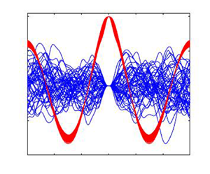
  $w_0$. In figure 2 the constraint of the maximum is absent. The figure shows the joint p.d.f. from (B1) together with an empirical p.d.f. based on 100 000 independent Slepian realisations.
Joint horizontal/vertical velocity depending on wave height for a J20 spectrum. (a) At wave max equal to  $w_0$. (b) At wave max exceeding $w_0$. (A/a)–(E/e): $w_0 = [0.25 \ 0.5\ 1\ 1.5\ 2] \times H_s$. The level curves enclose 10 : 20 : 90, 95, 99, 99.9 % of the distribution.

Joint density of  $v_h, v_v$, horizontal and vertical particle velocities at local maxima from (B1) (smooth, red curves) together with empirical p.d.f. from 100 000 simulated Slepian realisations (wiggly black curves). Level curves as in figure 1. The wave spectrum is J20 at infinite depth. The level curves enclose 10 : 20 : 90, 95, 99 % of the distribution.

4.3. Interpretation of the $q$-distribution (3.8) in the Gaussian case

In the following sections we will write  $A = W$ and $Z = W_{uu}$ for the random height and curvature of the maximum and express their joint density function (3.8) in explicit form,
 \begin{equation} q(z,a) =\frac{-z}{k} \exp\left\{-\frac{m_0 z^{2} + 2 m_{02}az + m_4a^{2}}{2(m_{0}m_{04}-m_{02}^{2})}\right\}, \quad z<0, \end{equation}
where  $k$ is a generic normalising constant. The following forms of the $q$-density are useful for simulation purposes:
 \begin{gather} q(z,a) = \frac{-z}{k} \exp\left\{-\frac{z^{2}}{2m_{04}} \right\} \times \exp\left\{-\frac{(a + z m_{02}/m_{04})^{2}}{2(m_0 - m_{02}^{2}/m_{04})} \right\},\quad z<0, \end{gather}
 \begin{gather}q(z \mid a) = \frac{-z}{k_a} \exp\left\{-\frac{(z + m_{02}a/m_0)^{2}}{2(m_{04}-m_{02}^{2}/m_0)} \right\},\quad z<0, \end{gather}
where  $k, k_a$ are normalising constants.
The first form is equivalent to the representation of  $W$ in (4.5) as the sum of a normal and a Rayleigh variable. The form (4.10) was used in Lindgren (Reference Lindgren1970) and it can be used to generate Slepian waves with fixed height $A=a$. We used simple rejection sampling by the Matlab routine sampleDist to simulate from this non-standard distribution.
4.4. Slepian models around wave crests
The Slepian model around a local maximum is defined from local characteristics, and the conditional distributions are defined explicitly in the Gaussian context. A more ‘regional’ wave definition is the one centred around the wave crests, i.e. the maxima between two successive mean level crossings. Any corresponding wave definition, like the trough–crest–trough wave or the zero–crest–zero half-wave, is complex involving non-local conditions. However, since any wave crest is also a local maximum, simulation of crest waves is easily performed by means of local maxima Slepian waves. One simply rejects those samples which do not satisfy the crest wave definition. In § 7.3 we will briefly investigate some of the complications and peculiarities that accompany this technique.
5. Functional structure of the Slepian processes
5.1. The regression functions and the residual functions
A Slepian model in a Gaussian model consists of one regression part with parameters determined by the random crossing event and one residual part for the variation around the regression. We base the models on representation (3.9), conditioning on the height  $A = W$ and the curvature $Z = W_{uu}$ at a local maximum, where $W_u=0$.
The Slepian processes for the  $W$- and $X$-components in the Gauss–Lagrange model have the structures
 \begin{gather} {\mathcal{W}}(u,t) = A \alpha^{w}(u,t) + Z \beta^{w}(u,t) + \varDelta^{w}(u,t), \end{gather}
 \begin{gather}{\mathcal{X}}(u,t) = A \alpha^{x}(u,t) + Z \beta^{x}(u,t) + \varDelta^{x}(u.t), \end{gather}
where the  $\alpha$- and $\beta$-functions are deterministic functions determined by the variances and covariances (A2) and (A3) and the $\varDelta$-functions are non-stationary, mean zero, correlated Gaussian fields, independent of $A$ and $Z$, whose density is (4.8). The joint distribution of the processes $\mathcal {W},\mathcal {X}$ in (5.1)–(5.2) is equal to the conditional distribution of $W, X$ around a local $W$-maximum in space. If we fix $A=a$ and generate $Z$ from (4.10) we get Slepian models near a wave with that height.
The next step is to describe the functions  $\alpha$ and $\beta$ and the covariances for the $\varDelta$-fields. The conditional distributions of $W(u,t), X(u,t)$ given the presence of a maximum at $\mathbf {0} = (0,0)$ are not normal. If we take the conditioning one step further and specify also the height and curvature at the maximum, the conditional distributions are again normal (Lindgren Reference Lindgren1972) and determined by conditional expectations and covariances. Thus we need only consider these functions for a pair of space–time points, $\boldsymbol {p}_j = (u_j, t_j)$, $j = 1,2$, separated by $\boldsymbol {p} = \boldsymbol {p}_2 - \boldsymbol {p}_1$.
In short, set  $\boldsymbol {W}_0= (W(\mathbf {0}), W_u(\mathbf {0}), W_{uu}(\mathbf {0}))$. The $7 \times 7$ partitioned covariance matrix of $(W(\boldsymbol {p}_1) \ W(\boldsymbol {p}_2) \mid X(\boldsymbol {p}_1) \ X(\boldsymbol {p}_2) \mid \boldsymbol {W}_0) = (\boldsymbol {W}, \boldsymbol {X}, \boldsymbol {W}_0)$, is
 \begin{align}
\varSigma &=
\begin{bmatrix} \varSigma_{\boldsymbol{W}\boldsymbol{W}} &
\varSigma_{\boldsymbol{W}\boldsymbol{X}} &
\varSigma_{\boldsymbol{W}\boldsymbol{W}_0}\\
\varSigma_{\boldsymbol{X}\boldsymbol{W}} &
\varSigma_{\boldsymbol{X}\boldsymbol{X}} &
\varSigma_{\boldsymbol{X}\boldsymbol{W}_0}
\\
\varSigma_{\boldsymbol{W}_0\boldsymbol{W}} &
\varSigma_{\boldsymbol{W}_0\boldsymbol{X}} &
\varSigma_{\boldsymbol{W}_0\boldsymbol{W}_0} \end{bmatrix}
\nonumber\\
&=\!\left(\! \begin{array}{cc | cc | ccc} m_{0}
& r^{ww}(\boldsymbol{p}) & r^{wx}(\mathbf{0}) &
r^{wx}(\boldsymbol{p}) & r^{ww}(\boldsymbol{p}_1) &
r^{w_uw}(\boldsymbol{p}_1) & r^{w_{uu}w}(\boldsymbol{p}_1)
\\ r^{ww}(\boldsymbol{p}) & m_{0} &
r^{wx}(-\boldsymbol{p}) & r^{wx}(\mathbf{0}) &
r^{ww}(\boldsymbol{p}_2) & r^{w_uw}(\boldsymbol{p}_2) &
r^{w_{uu}w}(\boldsymbol{p}_2) \\ \hline
r^{wx}(\mathbf{0}) & r^{wx}(-\boldsymbol{p}) & {\hat{m}}_0
& r^{xx}(\boldsymbol{p}) & r^{wx}(\boldsymbol{p}_1) &
r^{w_ux}(\boldsymbol{p}_1) & r^{w_{uu}x}(\boldsymbol{p}_1)
\\ r^{wx}(\boldsymbol{p}) &
r^{wx}(\mathbf{0}) & r^{xx}(\boldsymbol{p}) & {\hat{m}}_0 &
r^{wx}(\boldsymbol{p}_2) & r^{w_ux}(\boldsymbol{p}_2) &
r^{w_{uu}x}(\boldsymbol{p}_2) \\ \hline
r^{ww}(\boldsymbol{p}_1) & r^{ww}(\boldsymbol{p}_2) &
r^{wx}(\boldsymbol{p}_1) & r^{wx}(\boldsymbol{p}_2) & m_{0}
& 0 & - m_{02} \\
r^{w_uw}(\boldsymbol{p}_1) & r^{w_uw}(\boldsymbol{p}_2) &
r^{w_ux}(\boldsymbol{p}_1) & r^{w_ux}(\boldsymbol{p}_2) & 0
& m_{02} & 0 \\
r^{w_{uu}w}(\boldsymbol{p}_1) &
r^{w_{uu}w}(\boldsymbol{p}_2) &
r^{w_{u\!u}\!x}(\boldsymbol{p}_1) &
r^{w_{u\!u}\!x}(\boldsymbol{p}_2) & -m_{02} & 0 & m_{04}
\end{array} \!\right).
\end{align}
\begin{align}
\varSigma &=
\begin{bmatrix} \varSigma_{\boldsymbol{W}\boldsymbol{W}} &
\varSigma_{\boldsymbol{W}\boldsymbol{X}} &
\varSigma_{\boldsymbol{W}\boldsymbol{W}_0}\\
\varSigma_{\boldsymbol{X}\boldsymbol{W}} &
\varSigma_{\boldsymbol{X}\boldsymbol{X}} &
\varSigma_{\boldsymbol{X}\boldsymbol{W}_0}
\\
\varSigma_{\boldsymbol{W}_0\boldsymbol{W}} &
\varSigma_{\boldsymbol{W}_0\boldsymbol{X}} &
\varSigma_{\boldsymbol{W}_0\boldsymbol{W}_0} \end{bmatrix}
\nonumber\\
&=\!\left(\! \begin{array}{cc | cc | ccc} m_{0}
& r^{ww}(\boldsymbol{p}) & r^{wx}(\mathbf{0}) &
r^{wx}(\boldsymbol{p}) & r^{ww}(\boldsymbol{p}_1) &
r^{w_uw}(\boldsymbol{p}_1) & r^{w_{uu}w}(\boldsymbol{p}_1)
\\ r^{ww}(\boldsymbol{p}) & m_{0} &
r^{wx}(-\boldsymbol{p}) & r^{wx}(\mathbf{0}) &
r^{ww}(\boldsymbol{p}_2) & r^{w_uw}(\boldsymbol{p}_2) &
r^{w_{uu}w}(\boldsymbol{p}_2) \\ \hline
r^{wx}(\mathbf{0}) & r^{wx}(-\boldsymbol{p}) & {\hat{m}}_0
& r^{xx}(\boldsymbol{p}) & r^{wx}(\boldsymbol{p}_1) &
r^{w_ux}(\boldsymbol{p}_1) & r^{w_{uu}x}(\boldsymbol{p}_1)
\\ r^{wx}(\boldsymbol{p}) &
r^{wx}(\mathbf{0}) & r^{xx}(\boldsymbol{p}) & {\hat{m}}_0 &
r^{wx}(\boldsymbol{p}_2) & r^{w_ux}(\boldsymbol{p}_2) &
r^{w_{uu}x}(\boldsymbol{p}_2) \\ \hline
r^{ww}(\boldsymbol{p}_1) & r^{ww}(\boldsymbol{p}_2) &
r^{wx}(\boldsymbol{p}_1) & r^{wx}(\boldsymbol{p}_2) & m_{0}
& 0 & - m_{02} \\
r^{w_uw}(\boldsymbol{p}_1) & r^{w_uw}(\boldsymbol{p}_2) &
r^{w_ux}(\boldsymbol{p}_1) & r^{w_ux}(\boldsymbol{p}_2) & 0
& m_{02} & 0 \\
r^{w_{uu}w}(\boldsymbol{p}_1) &
r^{w_{uu}w}(\boldsymbol{p}_2) &
r^{w_{u\!u}\!x}(\boldsymbol{p}_1) &
r^{w_{u\!u}\!x}(\boldsymbol{p}_2) & -m_{02} & 0 & m_{04}
\end{array} \!\right).
\end{align} The conditional joint distribution of the processes  $W(u,t)$ and $X(u,t)$, given $\boldsymbol {W}_0 = (a, 0, z)$, is normal with mean and covariance
 \begin{align} &\begin{bmatrix} m_{w}(u,t) \\ m_{x}(u,t) \end{bmatrix} = \begin{bmatrix} r^{ww}(u,t) & r^{w_uw}(u,t) & r^{w_{uu}w}(u,t) \\ r^{wx}(u,t) & r^{w_ux}(u,t) & r^{w_{uu}\!x}(u,t) \end{bmatrix} \varSigma_{\boldsymbol{W}_0\boldsymbol{W}_0}^{{-}1} \begin{bmatrix}a \\ 0 \\ z\end{bmatrix}, \end{align}
 \begin{align} &{\mathsf{Cov}}(W(\boldsymbol{p}_1), W(\boldsymbol{p}_2), X(\boldsymbol{p}_1), X(\boldsymbol{p}_2) \mid \boldsymbol{W}_0)\nonumber\\ &\quad ={\mathsf{Cov}}(\varDelta^{w}(\boldsymbol{p}_1), \varDelta^{w}(\boldsymbol{p}_2), \varDelta^{x}(\boldsymbol{p}_1), \varDelta^{x}(\boldsymbol{p}_2)) \nonumber\\ &\quad =\begin{bmatrix} C_{\mathcal{W} \mathcal{W}} & C_{\mathcal{W} \mathcal{X}}\\ C_{\mathcal{X} \mathcal{W}} & C_{\mathcal{X} \mathcal{X}} \end{bmatrix} = \begin{bmatrix} \varSigma_{\boldsymbol{W}\boldsymbol{W}} & \varSigma_{\boldsymbol{W}\boldsymbol{X}}\\ \varSigma_{\boldsymbol{X}\boldsymbol{W}} & \varSigma_{\boldsymbol{X}\boldsymbol{X}} \end{bmatrix} - \begin{bmatrix}\varSigma_{\boldsymbol{W}\boldsymbol{W}_0} \\ \varSigma_{\boldsymbol{X}\boldsymbol{W}_0} \end{bmatrix} \varSigma_{\boldsymbol{W}_0\boldsymbol{W}_0}^{{-}1} (\varSigma_{\boldsymbol{W}_0\boldsymbol{W}} \ \varSigma_{\boldsymbol{W}_0\boldsymbol{X}}). \end{align}
 Evaluating (5.4) we get the conditional expectations of  $W(u,t)$ and $X(u,t)$ given a space maximum at $\mathbf {0}$ with height and curvature $A=a, Z=z$,
 \begin{equation} \left.\begin{gathered} m_w(u,t \mid a,z ) = \frac{a\left(m_{04} r^{ww}(u,t)+m_{02} r^{w_{uu}w}(u,t)\right) + z \left(m_{02} r^{ww}(u,t)+ m_0 r^{w_{uu}w}(u,t)\right)}{m_0m_{04}-m_{02}^{2}}, \\ m_x(u,t \mid a,z) = \frac{a\left(m_{04} r^{wx}(u,t)+m_{02} r^{w_{uu}x}(u,t)\right) + z \left(m_{02} r^{wx}(u,t)+ m_0 r^{w_{uu}x}(u,t)\right)}{m_0m_{04}-m_{02}^{2}}. \end{gathered}\right\}\end{equation}
 In (5.5) the off-diagonal elements in  $C_{\mathcal {W} \mathcal {W}}, C_{\mathcal {W} \mathcal {X}}, C_{\mathcal {X} \mathcal {X}}$ contain the conditional auto-covariance and cross-covariance functions for the normal residual processes. In the following, explicit expressions the time arguments $s, t$ can be changed to space arguments. For covariance functions in space–time one can use the notation $\boldsymbol {p}_j = (u_j, t_j)$, $j = 1,2$, separated by $\boldsymbol {p} = \boldsymbol {p}_2 - \boldsymbol {p}_1$ as in (5.3). The expressions in time only are
 \begin{align} C^{w}(s,t) &= {\mathsf{Cov}}(\varDelta^{w}(s), \varDelta^{w}(t)) = r^{w}(t-s)\nonumber\\ &\quad - \frac{m_0 r^{w_{uu}w}(s) r^{w_{uu}w}(t) + m_{02} r^{w}(s)r^{w_{uu}w}(t)}{m_0m_{04}-m_{02}^{2}} \nonumber\\ &\quad - \frac{m_{02} r^{w_{uu}w}(s)r^{w}(t) + m_{04}r^{w}(s) r^{w}(t)}{m_0m_{04}-m_{02}^{2}} - \frac{r^{w_{u}\!w}(s) r^{w_{u} w}(t)}{m_{02}}, \end{align}
 \begin{align} C^{x}(s,t) &= {\mathsf{Cov}}(\varDelta^{x}(s), \varDelta^{x}(t)) = r^{x}(t-s) \nonumber\\ &\quad - \frac{m_0 r^{w_{uu}x}(s) r^{w_{uu}x}(t) + m_{02} r^{wx}(s) r^{w_{uu}x}(t)}{m_0m_{04}-m_{02}^{2}}\nonumber\\ &\quad - \frac{m_{02} r^{w_{uu}x}(s) r^{wx}(t) + m_{04} r^{wx}(s) r^{wx}(t)}{m_0m_{04}-m_{02}^{2}} - \frac{r^{w_{u}x}(s) r^{w_{u}x}(t)}{m_{02}}, \end{align}
 \begin{align} C^{wx}(s,t) &= {\mathsf{Cov}}(\varDelta^{w}(s), \varDelta^{x}(t)) = r^{wx}(t-s) \nonumber\\ &\quad - \frac{m_0 r^{w_{uu}w}(s) r^{w_{uu}x}(t) + m_{02} r^{w}(s) r^{w_{uu}x}(t)}{m_0m_4-m_2^{2}} \nonumber\\ &\quad - \frac{m_{02} r^{w_{u}w}(s) r^{wx}(t) + m_{04} r^{w}(s) r^{wx}(t)}{m_0m_4-m_2^{2}} - \frac{r^{w_{u}w}(s) r^{w_{u}x}(t))}{m_{02}}. \end{align}
 One should be aware that there are four residual processes involved in the model:  $\varDelta ^{w}(u)$ and $\varDelta ^{x}(u)$ as space functions, and $\varDelta ^{w}(t)$ and $\varDelta ^{x}(t)$ as processes in time, and they are all dependent on each other.
5.1.1. Explicit Slepian models for the Gaussian components
We now formulate Slepian models for the Gaussian components conditioned on a local space maximum in  $W(u,0)$ at $u=0$, and from these we describe the Lagrangian wave shape and the corresponding particle orbit. Note that all $\varDelta$-processes are correlated through (5.9). The Slepian models for the components are, with the distribution of $A,Z$ given by (4.9) or, when $A$ is fixed, by (4.10)
 \begin{equation} \left.\begin{array}{ll@{}} \text{Wave models}: & {\mathcal{W}}(u,0) = m_w(u,0 \mid A,Z) + \varDelta^{w}(u,0) \\ & \qquad\quad\enspace = A\alpha^{w}(u,0) + Z \beta^{w}(u,0) + \varDelta^{w}(u,0),\\ & {\mathcal{X}}(u,0) = m_x(u,0 \mid A,Z) + \varDelta^{x}(u,0) \\ & \qquad\quad\enspace = A\alpha^{x}(u,0) + Z \beta^{x}(u,0) + \varDelta^{x}(u,0),\\ \text{Orbit models}: & {\mathcal{W}}(0,t) = m_w(0,t \mid A,Z) + \varDelta^{w}(0,t) \\ & \qquad\quad\enspace= A\alpha^{w}(0,t) + Z \beta^{w}(0,t) + \varDelta^{w}(0,t),\\ & \;{\mathcal{X}}(0,t) = m_x(0,t \mid A,Z) + \varDelta^{x}(0,t)\\ & \qquad\quad\enspace= A\alpha^{x}(0,t) + Z \beta^{x}(0,t) + \varDelta^{x}(0,t). \end{array}\right\} \end{equation}
 We note that with  $\rho = 1/\tanh (\kappa h)$,
 \begin{equation} \left.\begin{gathered} m_w(0,0 \mid a,z ) = a, \\ m_x(0,0 \mid a,z) = {\mathsf{E}}(X(0,0)) = 0, \\ C^{w}(0,0) = {\mathsf{V}}(\varDelta^{w}(0,0)) = 0, \\ C^{wx}(0,0) = {\mathsf{Cov}}(\varDelta^{w}(0,0),\varDelta^{x}(0,0)) = 0,\\ C^{x}(0,0) = {\mathsf{V}}(\varDelta^{x}(0,0)) =\int \rho^{2} S(\omega) \, \mathrm{d} \omega - \left.\left\{\int \rho \kappa S(\omega)\, \mathrm{d} \omega\right\}^{2}\right/m_{02}. \end{gathered}\right\} \end{equation}
This means that, at the maximum, the Slepian model for the wave is exactly equal to the height of the maximum, as it should be. The average displacement there is also zero, but randomly normal with non-zero variance, (5.11).
For easy reference we state the functional forms of the Slepian models, leaving out the redundant  $t=0$ and $u=0$, respectively,
 \begin{gather} \left.\begin{gathered} {\mathcal{W}}(u)= A\,\frac{m_{04} r^{ww}(u) + m_{02} r^{w_{uu}w}(u)}{m_0m_{04}-m_{02}^{2}} + Z\, \frac{m_{02} r^{ww}(u) + m_0 r^{w_{uu}w}(u))}{m_0m_{04}-m_{02}^{2}}+ \varDelta^{w}(u),\\ {\mathcal{X}}(u)= A\,\frac{m_{04} r^{wx}(u) + m_{02} r^{w_{uu}x}(u)}{m_0m_{04}-m_{02}^{2}} + Z\, \frac{m_{02} r^{wx}(u) + m_0 r^{w_{uu}x}(u))}{m_0m_{04}-m_{02}^{2}}+ \varDelta^{x}(u), \end{gathered}\right\}\end{gather}
 \begin{gather} \left.\begin{gathered} {\mathcal{W}}(t) = A\,\frac{m_{04} r^{ww}(t) + m_{02} r^{w_{uu}w}(t)}{m_0m_{04}-m_{02}^{2}} + Z\, \frac{m_{02} r^{ww}(t) + m_0 r^{w_{uu}w}(t))}{m_0m_{04}-m_{02}^{2}}+ \varDelta^{w}(t),\\ {\mathcal{X}}(t) = A\,\frac{m_{04} r^{wx}(t) + m_{02} r^{w_{uu}x}(t)}{m_0m_{04}-m_{02}^{2}} + Z\, \frac{m_{02} r^{wx}(t) + m_0 r^{w_{uu}x}(t))}{m_0m_{04}-m_{02}^{2}}+ \varDelta^{x}(t). \end{gathered}\right\}\end{gather}
The formulas are valid both when  $A,Z$ are jointly random with density (4.9) and when $A=a$ is fixed and $Z$ is random with conditional density (4.10).
6. Results: Gaussian Slepian models – wave shape and orbits
We illustrate the theory on the same orbital spectra as are used in (Lindgren & Prevosto Reference Lindgren and Prevosto2020). The spectrum J20 is a narrow JONSWAP spectrum with significant wave height  $H_s = 4.5$ m, peak period $T_p = 10$ s and $\gamma = 20$. The mean max–max wavelength is $40.4$ m and the mean zero crossing wavelength is $112$ m. The spectrum PM is a Pierson–Moskowitz wind–sea spectrum with $H_s = 4.5$ m, $T_p = 10$ s. Its max–max and mean zero crossing wavelengths are $16.1$ m and $71$ m, respectively. In the simulations the spectra are frequency truncated, the J20 spectrum at $2\ \textrm {rad}\ \textrm {s}^{-1}$ and the PM spectrum at $3\ \textrm {rad}\ \textrm {s}^{-1}$.
6.1. Slepian models in space – wave shape
Figure 3 shows 20 samples of the Slepian processes (5.12) for the J20 model on infinite depth conditioned on a local maximum in  $W(u,0)$ with height 4 m. Panel (a) shows realisations of the Gaussian wave form as a function of $u$ in an interval extending 50 m around the maximum. The red curves are the regression parts, i.e. the expected Slepian curves (5.6) while the blue curves include the normal residuals around the regression, as in (5.12). Panel (b) shows the horizontal displacement as a function of its original location relative to the maximum. In the simulations the maximum height was fixed to $a = 4$ m and the curvature distribution defined by conditioning in (4.10).
Slepian model realisations of Gaussian wave shape  ${\mathcal {W}}(u)$ (a) and horizontal displacement ${\mathcal {X}}(u)$ (b) according to (5.12) conditioned on a local maximum with height $a=4$ m. The narrow band of red curves shows the regression curves depending on the curvature at maximum, the more variable blue curves are full Slepian models including correlated residuals, independent of maximum height and curvature. The thick brown curves in the two panels come from the same realisation. The black dashed curve in the left plot represents a simplified regression, also called the ‘New Wave model’, i.e. $a r^{ww}(u,0)/r^{ww}(0,0)$. The spectrum is the JONSWAP spectrum J20.

The black dashed curve in figure 3 is the ‘New Wave model’, defined by Tromans et al. (Reference Tromans, Anaturk and Hagemeijer1991, equation (3)) as  $ar^{ww}(u,0)/r^{ww}(0,0)$, which is the expected (most probable) value conditioned on a stationary point at $u=0$, i.e. $W(0)=a, W'(0)=0$, regardless of its curvature. As soon as the curvature is involved, the functional form will be more complicated, (Lindgren Reference Lindgren1970, Theorem 3), and (5.6) in the present paper. However, it is easy to see from the conditional density (4.10) that $Z/a$ tends in probability to $-m_{02}/m_0$ as $a \to \infty$. Inserting this limit into the expectation in (5.6) we see that $m_w(u,0 \mid a,z)/a \to r^{ww}(u,0)/r^{ww}(0,0)$, i.e. our model is asymptotically equivalent to the Tromans model.
The residuals in figure 3 were simulated from the models (5.7)–(5.9) with dependence between  $\varDelta ^{w}(u')$ and $\varDelta ^{x}(u'')$. The residuals were generated by the WAFO-routine rndnormnd from their joint high-dimensional covariance matrix (WAFO-group 2017).
6.2. Slepian models in time – particle orbits and depth dependence
For the orbit model we need the Slepian models  ${\mathcal {X}}^{o}(t), {\mathcal {W}}^{o}(t)$ from (5.13). Figure 5(a) shows orbits from the same model as in figures 3 and 4. Figure 5(b) shows the variation in eccentricity at moderate depth $h = 30$ m. Here, we have an opportunity to compare the outcomes with classical wave theory that predicts the eccentric elliptic shape of water particles as a function of water depth. The Airy orbital eccentricity of surface particles is $\cosh (k_p h)/\sinh (k_p h)$ where $k_p$ is the peak wavenumber and $h$ is the water depth (Kinsman Reference Kinsman2002, p. 137). For the J20 spectrum at depth $h = 30$ m this measure takes the value 1.14, very close to the average eccentricity 1.12 of the regression orbits.
Slepian wave and displacement components for models in figure 3 plotted separately.

Orbits for the top particles in figure 3 according to models (5.13). (a) Infinite depth; (b) depth 30 m. Red curves are the symmetric regression orbits, blue dashed asymmetric curves include the residuals. The Airy orbital eccentricity of surface particles at water depth  $h=30$ m is $\cosh (k_p h)/\sinh (k_p h) =1.14$ for this narrow spectrum with peak frequency $\omega _p = 0.046\ \textrm {rad}\ \textrm {s}^{-1}$. The observed average eccentricity of the simulated regression orbits is 1.12.

7. Results: Slepian models in the Lagrange model
From (5.12) and (2.4) we can define a Slepian model for the Lagrange space wave at  $t_0=0$,
 \begin{equation} {\mathcal{L}}^{w}(x) ={\mathcal{L}}^{w}({\mathcal{X}}^{w}(u)) = {\mathcal{W}}^{w}(u), \end{equation}
valid in an interval  $x^{-} < x < x^{+}$ around $0$ where $u+{\mathcal {X}}^{W}(u)$ is strictly increasing. The model for the top particle orbit is defined directly from (5.13),
 \begin{equation} ({\mathcal{X}}^{o}(t) , {\mathcal{W}}^{o}(t)),\quad -\infty < t < \infty. \end{equation}
We are now ready to focus on the original goal for this paper: the statistical relation between local wave asymmetry and orbit orientation for the top particle in Lagrange waves.
7.1. Slepian model around local maxima
We use the same wave definition as in Lindgren & Prevosto (Reference Lindgren and Prevosto2020, § 3.1), namely the min–max–min definition and apply the Slepian model.
Consider a realisation of the Slepian model  ${\mathcal {W}}^{w}(u)$ with a maximum of height $a$ at $u=0$. Denote by $u^{-}<0 < u^{+}$ the locations of the local minima closest to $0$ and write $m^{-} = {\mathcal {W}}^{w}(u^{-})$ and $m^{+} = {\mathcal {W}}^{w}(u^{+})$ for their heights. After the Lagrange space shift by ${\mathcal {X}}^{w}$ the three extrema are located at ${\mathcal {X}}^{w}(u^{-}) <{\mathcal {X}}^{w}(0) <{\mathcal {X}}^{w}(u^{+})$, with order preserved if $u+{\mathcal {X}}^{w}(u)$ is strictly increasing in $u$. The wave front and back steepness are then defined by
 \begin{equation} \left.\begin{gathered} s^{+} = (a - m^{+})/({\mathcal{X}}^{w}(0) - {\mathcal{X}}^{w}(u^{+})) <0,\\ s^{-}= (a - m^{-})/({\mathcal{X}}^{w}(0) -{\mathcal{X}}^{w}(u^{-})) > 0. \end{gathered}\right\}\end{equation}
The front–back asymmetry is measured in logarithmic scale as  $\varLambda = \log (-s^{+}/s^{-})$; waves with positive $\varLambda$ have steep front and less steep back.
We define the orbit of the top particle as a function of  $\tau$,
 \begin{equation} O(\tau) = \left({\mathcal{X}}^{o}(\tau) , {\mathcal{W}}^{o}(\tau)\right),\quad -d^{-} \leqslant \tau \leqslant d^{+}, \end{equation}
where the interval is chosen so that  ${\mathcal {W}}^{w}(\tau )$ has local minima at $-d^{-}$ and $d^{+}$, these minima being the closest to $0$.
$0$.
7.2. Particle velocities, wave asymmetry and orbital orientation at local maxima
As a proxy for the orbital orientation one can fit an ellipse to the trajectory in the interval around the centre and use its orientation as a measure of orbit tilt. This was the approach in Lindgren & Prevosto (Reference Lindgren and Prevosto2020, § 3.3), where the Matlab routine fit $\_$ellipse was used to find the tilt $\theta _e$ of the approximating ellipse as a measure of the orbit orientation. It was suggested in that paper that the velocity vector for the top particle would give a more objective measure of the connection between wave asymmetry and orbit orientation. Intuitively, an upward direction would indicate an upward tendency of the orbit and vice versa, and as a local variable it would not be subject to the wild randomness of the orbit.
For the top particle orbits we observe that the maximum in space,  ${\mathcal {W}}^{w}(0)$, is not a maximum in time. We use the velocities $v_v = {\mathcal {W}}^{o}_t(0)$ and $v_h = {\mathcal {X}}^{o}_t(0)$ to calculate the velocity direction $\theta _v = {\textrm {atan2}} (v_v,v_h)$. According to (4.5) $v_v$ is normal and independent of $v_h$, which in turn is the sum of one normal and one Rayleigh variable; its p.d.f. is given in Fact B.1 in Appendix B.
Figure 2 shows the theoretical joint p.d.f. of  $v_h, v_v$ for all local maxima and it agrees with simulations from 100 000 simulated Slepian realisations. As seen, they are centred at a positive average horizontal velocity while the vertical one is symmetric around zero. We now investigate the relation to the wave geometry.
We simulate Slepian processes from JONSWAP (J20) and Pierson–Moskowitz (PM) spectra at different depths and observe the Lagrange wave skewness from (7.3). For the orbit orientation we observe both the velocity direction  $\theta _v$ of the top particle and the orientation $\theta _e$ of the fitted ellipse as measures of orbit tilt. We compare with the results in Lindgren & Prevosto (Reference Lindgren and Prevosto2020, figure 7a–c) where waves and orbits were observed in simulated space series. Figure 6 shows the J20 results from simulated Slepian realisations at infinite depth and depths of $h = 40, 20$ m. As in the cited work we restricted the data to ‘major’, waves with maximum height exceeding $H_s/8$ and front and back amplitudes greater than $H_s/4$. Figure 7 can be compared to figures 2 and 5 in Lindgren & Prevosto (Reference Lindgren and Prevosto2020), showing the corresponding results for the PM spectrum.
Relation between wave asymmetry and orbit orientation for J20 waves. (a,c,e) Orbit orientation measured by fitted ellipse. (b,d,f) Orbit orientation measured by velocity vector of top particle. Depth from top: infinite,  $h=40$ m, $h=20$ m. Simulation data with 8000, 9000, 14 000 wave/orbit pairs.

Relation between wave asymmetry and orbit orientation for PM waves. (a,c,e) Orbit orientation measured by fitted ellipse. (b,d,f) Orbit orientation measured by velocity vector of top particle. Depth from top: infinite,  $h=40$ m, $h=20$ m. Simulation data with approximately 8000, 8000, 9000 wave/orbit pairs.

One can draw the immediate conclusion that both orientation measures have a strong but different statistical relation to the wave asymmetry. Panels (a,c,e) in figures 6 and 7 relate the wave asymmetry to the tilt of the ellipse fitted to the orbit. Panels (b,d,f) show the well-behaved correlation between asymmetry and top velocity orientation. The depth dependence in the tilt measure is much less present in the velocity measure, indicating that the former is partly due to the irregularity of the full orbits, which become more ellipse like with decreasing depth.
7.3. Slepian models for half waves
By ‘half-crest wave’ (‘crest wave’ for short) we mean a section of the space or time wave that lies between a mean level upcrossing and the following downcrossing. The crest is the largest local maximum of the half-wave. Since the crest also is a local maximum one can use the Slepian model for local maxima to propose a Slepian crest wave, a proposal that is rejected if it is not the maximum between the nearest mean level crossings.
For the Lagrange space waves, the skewness and max particle orbits for half-crest waves are defined as follows, with notations similar to those in § 7.1. A pair of Slepian realisations  ${\mathcal {W}}(u,t), {\mathcal {X}}(u,t)$ is accepted as part of a Lagrange crest wave if ${\mathcal {W}}(u,0)$ is the maximum ${\mathcal {W}}$ between the nearest upcrossing and downcrossing zeros $u^{-}<0< u^{+}$ on either side at time of observation
 \begin{equation} \left.\begin{gathered} A = {\mathcal{W}}(0,0) > {\mathcal{W}}(u,0) > 0, \quad u^{-} < u < u^{+}, \\ 0 = {\mathcal{W}}(u^{-},0) = {\mathcal{W}}(u^{+},0). \end{gathered}\right\} \end{equation}
The Lagrange wave steepness is defined by analogy to (7.3),
 \begin{equation} \left.\begin{gathered} s^{+} = A/({\mathcal{X}}^{w}(0,0) - {\mathcal{X}}^{w}(u^{+},0)) <0,\\ s^{-} = A/({\mathcal{X}}^{w}(0,0) -{\mathcal{X}}^{w}(u^{-},0)) > 0, \end{gathered}\right\} \end{equation}
which simplifies the skewness measure to  $\varLambda = \log (-({{\mathcal {X}}^{w}(0,0) - {\mathcal {X}}^{w}(u^{-},0)})/ ({{\mathcal {X}}^{w}(0,0) -{\mathcal {X}}^{w}(u^{+},0)}))$.
As suggested in Lindgren & Prevosto (Reference Lindgren and Prevosto2020, § 3) the crest wave definition will lead to more chaotic orbits with extra twists and to less characteristic wave skewness measures. We verify this claim and present some of the reasons.
One disturbing random factor is the presence and location of local maxima in the crest wave, besides the crest maximum. The number and allocation of these extra maxima represent a discrete source of disturbing randomness in the skewness measure as can be understood from figure 8. The skewness distribution will be a discrete mixture of continuous distributions. For example, configuration 1–1 will tend to be centred at  $0$ while 1–0 and 0–2 will be centred near a distinct negative and positive value, respectively.
Illustration of the discrete dependence of crest location (marked with  $\times$) and the number of local maxima in a crest period. The code $x$–
$x$– $y$ indicates the number of local maxima to the left and right of the crest, respectively.

The probability of extra maxima increases with the length of the crest interval. For the J20 JONSWAP spectrum, used in this example, the distribution of the interval length is strongly bimodal, with one peak near 10 m and one near 40 m, enhancing the mixture effect; figure 9. For the PM spectrum, the crest interval distribution has a sharp peak for short intervals and a flat part between 30 and 50 m, enough to cause a discrete skewness measure.
Probability densities of crest wavelength for PM (solid, blue) and J20 (dashed, red) spectra, computed by the WAFO routine spec2tpdf, (WAFO-group 2017).

The probability of extra maxima in a crest wave is also related to the height of the crest. Small crests have approximately a parabolic shape, (Slepian Reference Slepian1963, § 3), with asymptotically equal front and back periods, leading to an asymmetry measure near zero. This introduces an extra disturbance in the relation between wave asymmetry and top particle direction as is seen in figure 10. The figure shows simulated pairs of top particle directions and wave asymmetry for crest waves with only one local maximum. Blue dots illustrate the distribution with all maxima included, black dots show pairs with maximum above 3 m, and red dots come from small waves with height less than 0.1 m. Simulations from the PM spectrum give the same type of crest height dependence.
Remark 7.1 Slepian simulation of crest waves can be made by the original simple Slepian model after mean level upcrossings and crest height and location as well as front and back periods observed in the realisations. This method is very fast and it gives the same results for the wave geometry as the method we use here, but it does not give any information on the top particle velocities.
Illustration of the dependence of crest height on the relation between top particle direction and crest wave skewness, J20 spectrum.

8. Discussion
Our analysis gives rise to several questions that need to be discussed, and here we address two: the effect of second-order Stokes corrections and the importance of crest height.
Wave crest–trough asymmetry: the Gauss–Lagrange waves exhibit crest–trough asymmetry very similar to that in second- and higher-order Stokes models (Tayfun Reference Tayfun1980) but the mechanisms are fundamentally different. In the Stokes model, wave crests become more peaked and troughs are flattened by the addition of frequency interaction terms. In the Gauss–Lagrange model crests and troughs present in the vertical Gaussian component remain crests and troughs after the horizontal displacement and their heights are unaltered. Crests are narrowed and troughs flattened by the displacement.
Wave front–back asymmetry: the focus in this paper is on the relation between the stochastic variation of wave front–back asymmetry and the direction of the crest top particle. A relevant question regards how the derived relation changes when Stokes terms are added to the wave profiles. For the spectra we have used, the standard deviation of the vertical and horizontal effects of the second-order Stokes correction is 5 %–10 % of those of the Gaussian terms and the effect on wave asymmetry is small. For the crest particle velocity the effects are similarly small. For the J20 spectrum the Stokes term causes large but slow horizontal oscillating drifts, the standard deviation of the added horizontal velocity is approximately 10 % of the Gaussian velocity. The vertical velocity is not affected. For the PM spectrum the effects of the Stokes correction are even smaller. The effect on the asymmetry–velocity relations in figures 6 and 7 is small.
Stokes drift: as observed in Lindgren & Prevosto (Reference Lindgren and Prevosto2020, § 3.4) the Stokes drift has a very small effect on the wave asymmetry but it has a systematic effect on the horizontal particle velocity. The effect depends on the crest height and is of smaller order than the model velocity illustrated in figure 1.
Dependence on crest height: it is worth noting that the residual process in the Slepian models does not depend on the crest height. Close to the maximum its variability is very small but it increases abruptly with distance from the crest and overshadows the regression term, which is proportional to the maximum height. This is illustrated in figure 11.
Height dependence illustrating the balance between the variability of regression (red smooth curves) and residual (blue irregular curves) for different crest heights  $a$. Sea state is the J20 model.

9. Summary and conclusions
We have shown how a Slepian model can be used for detailed studies of the front–back asymmetry of irregular ocean waves and how wave asymmetry is related to the kinematics of the particle near wave maxima in space. Based on Gaussian field models for the Lagrangian vertical and horizontal particle movements we present explicit expressions for the complete distribution of the local wave process and for the random top particle orbit, as well as for their joint statistical distribution. Examples from two very different wave spectra, one narrow JONSWAP spectrum and one Pierson–Moskowitz wind–wave spectrum, show that there is a stable systematic covariation between the orientation of the top particle movement and the degree of front–back asymmetry. The relation is not sensitive to deviations from the Gaussian assumptions and could be empirically adapted to field observations of particle kinematics.
The Slepian model is a very versatile tool for detailed analysis of crossing related events in a stochastic process or field. It is explicit and very easy and fast to simulate and it lends itself to analysis also of very rare events. In our analysis we derived a Slepian model for individual space waves defined as the part of the surface between two local minima with the wave centred at the intermediate local maximum. A companion model is given for the particle orbits, i.e. the horizontal movements in time for the particle located at the wave maximum. Both models include the height and the curvature at the wave maximum as random parameters in a deterministic regression part surrounded by non-stationary Gaussian residual processes. The variability of the residual compared with that of the regression gives a hint of how far away from the wave maximum one can expect to draw reliable conclusions. As it is locally defined, the top particle orientation is a stable measure of orbit orientation and its covariation with wave asymmetry is not affected by the non-local residual variability.
As an alternative to the min–max–min wave definition we also used the Slepian technique to the crest half-wave definition, used in our previous study of the asymmetry–orbit relation, (Lindgren & Prevosto Reference Lindgren and Prevosto2020). We conclude here that the top particle method can give more stable relations to the wave asymmetry than the ellipse tilt method used in the previous paper, but that the presence of extra local maxima disturbs the clear relation. We identified the bi-modality of the crest wavelength distribution as an important factor, complicating the relation between wave asymmetry measure and orbit orientation.
Slepian models have great potential in ocean wave modelling, and we finish with two recent examples where a Slepian formulation might be fruitful.
The first example concerns wave breaking, a highly nonlinear phenomenon. Waves obtained from Gaussian modelling are far from the extreme nonlinear waves that are encountered close to breaking conditions. On the other hand, Gaussian modelling permits one to obtain statistical distributions for extreme combinations of random quantities characteristic for ‘real world’ nonlinearities derived from deterministic nonlinear wave equations. For example, in this way, Stringari et al. (Reference Stringari, Prevosto, Filipot, Leckler and Guimarães2021) derive wave breaking probabilities based on a crest particle velocity–speed of local maxima ratio criterion. Applied to classical wave breaking criteria, the new formula compares well with historical methods on recorded data. The second example (Hlophe et al. Reference Hlophe, Wolgamot, Kurniawan, Taylor and Orszaghova2021) concerns wave-to-wave prediction in weakly nonlinear wave fields, where crossing conditioning could be useful.
Acknowledgements
This research received no specific grant from any funding agency, commercial or not-for-profit sectors.
Declaration of interests
The authors report no conflict of interest.
Appendix A. Some moments and covariance functions
We need the following moments and covariance functions for the  $W$- and $X$-fields and their derivatives, for example
 \begin{equation} W_u(0,0) = \frac{\partial W(u,t)}{\partial u} (0,0), \quad W_{uu}(0,0) = \frac{\partial^{2} W(u,t)}{\partial u^{2}} (0,0). \end{equation}
We use a one-sided orbital spectrum  $S(\omega ), \omega > 0$ with notations $\gamma = \kappa u - \omega t$ and $\rho = 1/\tanh (\kappa h)$,
 \begin{gather} \left.\begin{gathered} m_0 = {\mathsf{V}}(W(0,0)) = \int S(\omega) \, \mathrm{d} \omega,\\ m_{02} = {\mathsf{V}}(W_u(0,0)) = \int \kappa^{2} S(\omega)\, \mathrm{d} \omega,\\ m_{04} = {\mathsf{V}}(W_{uu}(0,0)) = \int \kappa^{4} S(\omega)\, \mathrm{d} \omega,\\ m_{20} = {\mathsf{V}}(W_t(0,0)) = \int \omega^{2} S(\omega)\, \mathrm{d} \omega, \\ m_{11} ={-}{\mathsf{Cov}}(W_u(0,0), W_t(0,0)) = \int \omega \kappa \, S(\omega)\, \mathrm{d} \omega,\\ {\hat{m}}_0 = {\mathsf{V}}(X(0,0)) = \int \rho^{2} S(\omega) \, \mathrm{d} \omega,\\ {\hat{m}}_{10} = {\mathsf{Cov}}(W(0,0), X_t(0,0)) = \int \rho \omega S(\omega)\,\mathrm{d} \omega,\\ {\hat{m}}_{20} = {\mathsf{V}}(X_t(0,0)) = \int \rho^{2} \omega^{2}S(\omega)\,\mathrm{d} \omega,\\ {\hat{m}}_{12} ={-}{\mathsf{Cov}}(W_{uu}(0,0), X_{t}(0,0))= \int \rho \omega \kappa^{2} S(\omega)\, \mathrm{d} \omega, \end{gathered}\right\}\end{gather}
 \begin{gather} \left.\begin{gathered} r^{ww}(u,t) = {\mathsf{Cov}}(W(0,0), W(u,t)) = \int \cos (\gamma) S(\omega) \, \mathrm{d} \omega,\\ r^{xx}(u,t) = {\mathsf{Cov}}(X(0,0), X(u,t)) = \int \rho^{2} \cos (\gamma) S(\omega) \, \mathrm{d} \omega,\\ r^{wx}(u,t) = {\mathsf{Cov}}(W(0,0),X(u,t)) ={-} \int \rho \sin (\gamma) S(\omega)\, \mathrm{d} \omega,\\ r^{w_uw}(u,t) = {\mathsf{Cov}}(W_u(0,0),W(u.t)) = \int \kappa \sin(\gamma) S(\omega) \,\mathrm{d} \omega, \\ r^{w_u x}(u,t) = {\mathsf{Cov}}(W_u(0,0),X(u,t)) = \int \rho \kappa \cos(\gamma) S(\omega) \, \mathrm{d} \omega, \\ r^{w_{uu} w}(u,t) = {\mathsf{Cov}}(W_{uu}(0,0),W(u,t)) ={-} \int \kappa^{2} \cos(\gamma) S(\omega) \, \mathrm{d} \omega, \\ r^{w_{uu}x}(u,t) = {\mathsf{Cov}}(W_{uu}(0,0), X(u,t)) = \int\rho \kappa^{2} \sin(\gamma) S(\omega) \, \mathrm{d} \omega. \end{gathered}\right\}\end{gather}
Appendix B. Rayleigh shifted normal distributions
A Slepian process in Gaussian models normally consists of the sum of a Rayleigh variable and an independent normal variable or process. We present here the general expression for the p.d.f. of such a sum of variables. The formula for a single normal variable was originally given by Rice (Reference Rice1945, § 3.6), and it reads in general form (Lindgren Reference Lindgren2013, equation (8.37)) as in the following fact B.1.
Fact B.1 The probability density for the sum of a mean zero normal variable and an independent Rayleigh variable,  $Z = \sigma _1 N + \sigma _2 R$, with standard $N \sim N(0,1)$, $R \sim Ray(1)$, is, with $\varPhi$ the standard normal distribution function,
 \begin{align} f_Z(z) &= \frac{\sigma_2 z}{(\sigma_1^{2}+\sigma_2^{2})^{3/2}} \exp\left({- \frac{z^{2}}{2(\sigma_1^{2}+\sigma_2^{2})}}\right) \varPhi\left(\frac{\sigma_2 z}{\sigma_1\sqrt{\sigma_1^{2} + \sigma_2^{2}}}\right)\nonumber\\ &\quad + \frac{\sigma_1}{\sqrt{2 {\rm \pi}}(\sigma_1^{2} + \sigma_2^{2})} \exp\left({-\frac{z^{2}}{2\sigma_1^{2}}}\right). \end{align}
Fact B.2 Let  $\boldsymbol {X} = \left [\begin {smallmatrix}X_1 \\ X_2\end {smallmatrix}\right ]$ have a bivariate normal distribution with mean zero and covariance matrix $\varSigma$ and let $R$ be a standard Rayleigh variable, independent of $\boldsymbol {X}$. Define the Rayleigh translated normal variable
 \begin{equation} \boldsymbol{Y} = \boldsymbol{X} + R \begin{bmatrix}1\\1\end{bmatrix}, \end{equation}
with density as the convolution
 \begin{equation} f_{\boldsymbol{Y}}(\boldsymbol{y}) = \int_0^{\infty} r e^{{-}r^{2}/2} \times \frac{1}{2 {\rm \pi}\sqrt{\det \varSigma}} \exp\left\{- \frac 12 (\boldsymbol{y}-\boldsymbol{r})'A(\boldsymbol{y}-\boldsymbol{r})\right\} \mathrm{d} r, \end{equation}
where  $A = \varSigma ^{-1} = \left [\begin {smallmatrix}a_{11} & a_{12}\\a_{12} & a_{22}\end {smallmatrix}\right ]$. Expanding the quadratic form
 \begin{align} (\boldsymbol{y}-\boldsymbol{r})' A (\boldsymbol{y}-\boldsymbol{r}) &= a_{11} y_1^{2} + 2 a_{12} y_1y_2 + a_{22} y_2^{2} \nonumber\\ &\quad - 2 r \left(a_{11} y_1 + a_{12} (y_1+y_2) + a_{22} y_2\right) + r^{2} \left(a_{11} + 2a_{12} + a_{22}\right) \nonumber\\ &= \alpha(y_1,y_2) - 2 \beta(y_1,y_2) r + \gamma r^{2} = \alpha - \beta^{2}/\gamma + \gamma (r - \beta/\gamma)^{2}, \end{align}
we get
 \begin{align} f_{\boldsymbol{Y}}(\boldsymbol{y}) &= \int_0^{\infty} r \exp\{{-}r^{2}/2\} \times \frac{\sqrt{\gamma}}{\sqrt{2 {\rm \pi}}} \exp\left\{-\frac{\gamma}{2} (\beta/\gamma - r)^{2}\right\} \mathrm{d} r \nonumber\\ &\quad \times \frac{1}{\sqrt{2{\rm \pi} \gamma \det \varSigma}} \exp\left\{-\frac 12 (\alpha-\beta^{2}/\gamma)\right\}. \end{align}
The first factor is the convolution of a Rayleigh density and a normal density with mean 0 and variance  $1/\gamma$, i.e. it is equal to the p.d.f. (B1) with $\sigma _2=1$ of $R + N/\sqrt {\gamma }$ evaluated at $\beta /\gamma$, while the second factor is explicit. To apply the formula to the distribution in (4.5) we just normalise the relevant equations.


 Open access