





1. Introduction
Demersal fishes that live and forage near the seabed are ubiquitous in coastal and shallow-water environments (Moyle & Cech Reference Moyle and Cech2004; Gibson, Stoner & Ryer Reference Gibson, Stoner and Ryer2014; Fox et al. Reference Fox, Gibb, Summers and Bemis2018). Adapted to such near-bottom habitats, numerous demersal species have evolved specialised locomotion strategies. For instance, the winter flounder (Pleuronectes americanus) remains extremely close to the seabed during locomotion, rarely ascending more than one and a half body lengths above the bottom, and frequently swimming with its posterior body nearly in contact with the substrate (He Reference He2003). For demersal fishes, locomotion performance is determined not only by body kinematics but also by the benthic boundary and attached flexible structures, such as seagrass and macroalgae (Stoner & Titgen Reference Stoner and Titgen2003; O’Leary et al. Reference O’Leary, Goodman, Walter, Willits, Pondella and Stephens2021). Understanding how demersal fishes interact with the seabed therefore provides fundamental insights into physical mechanics governing benthic swimming, and inspires the design of underwater robots operating in near-boundary environments (Liu et al. Reference Liu, Ding, Pan, Yu, Lu, Chen, Zhang and Wang2024).
The influence of the seabed (bottom wall) on fish locomotion is termed the ground effect, which modulates both the body kinematics and propulsive performance of swimmers. For instance, the tail-beat amplitude and maximum swimming velocity of steelhead trout (Oncorhynchus mykiss) decrease when swimming near the seabed, while their tail-beat frequency remains unchanged (Webb Reference Webb1993). For the plaice (Pleuronectes platessa), a typical benthic fish, its tail-beat frequency increases with swimming velocity when moving near the seabed, but becomes independent of the velocity when swimming farther from the bottom (Webb Reference Webb2002). Similarly, Nowroozi et al. (Reference Nowroozi, Strother, Horton, Summers and Brainerd2009) observed that northern spearnose poacher (Agonopsis vulsa) use the ground effect to enhance lift when swimming within one centimetre of the seabed, thereby counteracting negative buoyancy. In a separate study, Yang et al. (Reference Yang, Li, Du, Wan, Jia, Yang and Zhang2024) reported that brown trout (Salmo trutta) exhibit increased swimming velocity but decreased propulsive efficiency when their distance from the seabed is less than half a body length.
Despite the inherently three-dimensional (3-D) nature of fish swimming, it is widely recognised that the leading-order propulsive mechanisms are predominantly governed by the unsteady lateral motion of the tail and the associated vortex dynamics developing in the plane normal to the spanwise direction of the caudal fin (Smits Reference Smits2019). Within this context, two-dimensional (2-D) models have been widely adopted as a minimal yet physically representative framework for investigating fish-like propulsive dynamics (Alben Reference Alben2008; Alben et al. Reference Alben, Witt, Baker, Anderson and Lauder2012; Zhu, He & Zhang Reference Zhu, He and Zhang2014).
To explore the ground effect on flatfish-like propulsion, where the caudal fin primarily undergoes vertical oscillations above the seabed, aerofoils and flexible plates flapping near a rigid flat wall have been extensively studied. Employing both experimental and numerical methods, Quinn et al. (Reference Quinn, Moored, Dewey and Smits2014) investigated the hydrodynamic effects of a flat bottom wall on a rigid pitching aerofoil submerged in a free-stream flow. They observed that the average thrust of the aerofoil increases monotonically as the distance from the wall decreases, and further noted that concentrated vortices in the wake form upward-deflected vortex pairs rather than a reverse Bénard–von Kármán vortex street, thereby forming a mean momentum jet angled away from the wall. Additionally, an equilibrium height at which the average lift of the aerofoil attains zero has also been identified (Zhong et al. Reference Zhong, Han, Moored and Quinn2021; Han et al. Reference Han, Zhong, Mivehchi, Quinn and Moored2024). Numerical studies on self-propelled flexible plates near a flat wall in a quiescent flow have been conducted by Dai, He & Zhang (Reference Dai, He and Zhang2016), Tang et al. (Reference Tang, Huang, Gao and Lu2016), Park, Kim & Sung (Reference Park, Kim and Sung2017) and Zhang, Huang & Lu (Reference Zhang, Huang and Lu2017). These investigations revealed that in most cases, a rigid plate achieves a higher propulsive velocity near the bottom wall at the expense of increased energy consumption. However, a flexible plate with optimal stiffness exhibits enhancements in both propulsive velocity and energy efficiency. Jeong, Lee & Park (Reference Jeong, Lee and Park2021) further explored the collective motion of two tandem self-propelled flexible plates in the presence of zero, one or two side walls. They observed that the following plate exhibits a hybrid vortex interception–slalom locomotion pattern when side walls are present, which differs from the pure vortex interception mode observed without side walls. Furthermore, the overall efficiency of the plate pair is optimised under moderate wall proximity and bending rigidity.
It should be noted that the natural seabed is composed of sand, mud and aquatic vegetation (Van Katwijk et al. Reference Van Katwijk, Bos, Hermus and Suykerbuyk2010), which exhibit pronounced fluid-induced deformations. In vegetative flows, coherent waving motions between adjacent plants emerge under certain conditions, a phenomenon known as monami (Ackerman & Okubo Reference Ackerman and Okubo1993). Both experimental observations (Ghisalberti & Nepf Reference Ghisalberti and Nepf2002; Fu et al. Reference Fu, He, Huang, Dey and Fang2023) and numerical simulations (Huang, Shin & Sung Reference Huang, Shin and Sung2007; Zhang et al. Reference Zhang, He and Zhang2020b ) indicate that the onset and evolution of monami are predominantly governed by 2-D shear-layer instabilities, making 2-D blade models effective for capturing the essential flow–vegetation coupling mechanisms. O’Connor & Revell (Reference O’Connor and Revell2019) investigated coupled interactions between large arrays of 2-D slender blades in open-channel flow, identifying three distinct motion modes (static, regular waving and irregular waving) primarily driven by the flow. Ni et al. (Reference Ni, Zhang, Ji, Xu and Zhang2025) simulated the evolution of large-scale vortices above the vegetation canopy in a 2-D laminar flow, and found that the characteristics of vegetation swaying vary synchronously with those of large-scale vortices. Furthermore, turbulent flow over the vegetation canopy has also been studied to explore the interaction between multi-scale vortical structures and coherent motions of vegetation (Tschisgale et al. Reference Tschisgale, Löhrer, Meller and Fröhlich2021; He, Liu & Shen Reference He, Liu and Shen2022; Wang et al. Reference Wang, He, Dey and Fang2022a , Reference Wang, He, Dey and Fangb ; Foggi Rota et al. Reference Foggi Rota, Monti, Olivieri and Rosti2024).
While the hydrodynamics of near-wall swimming and the flow-induced motion of aquatic vegetation have been extensively studied in isolation, their bidirectional coupling remains poorly understood. On the one hand, fish swimming acts as a source of flow perturbation that inevitably modulates seagrass motion. On the other hand, vegetation response not only serves as an indicator of the swimmer’s locomotion, but also reciprocally affects the swimmer’s propulsive performance (Dibble, Killgore & Harrel Reference Dibble, Killgore and Harrel1996). Therefore, the present study aims to investigate the dynamic interaction between a self-propelled plate (representing a flatfish-like swimmer) and multiple wall-mounted compliant blades (representing aquatic vegetation), mimicking the scenario of a fish swimming over the vegetation canopy. Specifically, this study seeks to address the following two fundamental questions. First, how does the presence of compliant blades modify the propulsive performance of a self-propelled plate near the wall? Second, how does the flapping motion of the plate excite and organise the vibration response of the compliant blade array? These investigations are intended to advance the understanding of the physical mechanisms underlying the complex fluid–structure interaction between fish and their surrounding environment, thereby providing insights into the design of bio-inspired underwater vehicles and flow sensing techniques.
The remainder of the paper is organised as follows. Section 2.1 establishes the physical model and presents the mathematical formulations, while numerical methods and validation are presented in § 2.2. Section 3 presents the results, including the time-dependent flow (§ 3.1), propulsive performance of the self-propelled plate (§ 3.2), motion of the compliant blades (§ 3.3), and resonance between the plate and the blades (§ 3.4). The key findings are summarised in § 4.
2. Methodology
2.1. Problem set-up and governing equations
We consider a system consisting of a self-propelled flexible plate swimming above an array of wall-mounted compliant blades, as shown in figure 1. The plate and blades are immersed in an initially stationary viscous incompressible fluid. The self-propelled plate, with length $L$
, exhibits a zero tangential angle and a prescribed heaving motion at its leading edge. The vertical position of the leading edge, denoted as
$L$
, exhibits a zero tangential angle and a prescribed heaving motion at its leading edge. The vertical position of the leading edge, denoted as $y_l$
, is given by
$y_l$
, is given by
 \begin{equation} y_l(t)=a \sin {(2 \pi t/T+\pi )} + H, \end{equation}
where $a$
is the heaving amplitude,
$a$
is the heaving amplitude, $T$
is the period of the heaving motion, and
$T$
is the period of the heaving motion, and $H$
is the average height of the plate above the bottom wall (where
$H$
is the average height of the plate above the bottom wall (where $y=0$
). The compliant blades, initially mounted vertically on the bottom wall, have uniform height
$y=0$
). The compliant blades, initially mounted vertically on the bottom wall, have uniform height $L$
, constant spacing
$L$
, constant spacing $D$
, and total number
$D$
, and total number $N$
. Additionally, we assume that the thicknesses of both the plate and the blade are negligibly small.
$N$
. Additionally, we assume that the thicknesses of both the plate and the blade are negligibly small.
In the system, the fluid motion is governed by the incompressible Navier–Stokes equations and the continuity equation as
 \begin{align} \frac {\partial \boldsymbol{u}}{\partial t} + \boldsymbol{u}\boldsymbol{\cdot }\boldsymbol{\nabla }\boldsymbol{u} &= -\frac {1}{\rho } \boldsymbol{\nabla } p+\nu\, {\nabla} ^2 \boldsymbol{u}+\frac {1}{\rho }\boldsymbol{f}_{\textit{IB}}, \end{align}
 \begin{align} \boldsymbol{\nabla } \boldsymbol{\cdot }\boldsymbol{u} &= 0, \end{align}
where $\boldsymbol{u}$
is the fluid velocity,
$\boldsymbol{u}$
is the fluid velocity, $p$
is the static pressure,
$p$
is the static pressure, $\rho$
is the fluid density, and
$\rho$
is the fluid density, and $\nu$
is the kinematic viscosity. Here,
$\nu$
is the kinematic viscosity. Here, $\boldsymbol{f}_{\textit{IB}}$
is the volume force introduced in the immersed boundary method. The velocity is set to zero on the four boundaries of the computational domain, and a no-slip boundary condition is applied to the plate and blades. The flow is initially stationary throughout the computational domain.
$\boldsymbol{f}_{\textit{IB}}$
is the volume force introduced in the immersed boundary method. The velocity is set to zero on the four boundaries of the computational domain, and a no-slip boundary condition is applied to the plate and blades. The flow is initially stationary throughout the computational domain.
Schematic diagram for the self-propelled plate moving above an array of wall-mounted compliant blades.

Figure 1. Long description
The schematic diagram illustrates a self-propelled plate moving above an array of wall-mounted compliant blades. The diagram features a horizontal plane divided into sections labeled with dimensions. The plate is positioned above an array of vertical blades, which are uniformly spaced and attached to the bottom of the plane. The blades have a height labeled as L and a spacing labeled as D. The plate is shown at a height of H above the base, with a section of 5L on either side of the array. The array itself spans a length of 70L. The plate is depicted with a slight upward curvature, indicating a movement with a vertical displacement of 2a over a length L. The x and y axes are marked at the bottom left corner, indicating the coordinate system used in the diagram.
Following the approach of Connell & Yue (Reference Connell and Yue2007), Hua, Zhu & Lu (Reference Hua, Zhu and Lu2013) and Peng et al. (Reference Peng, Sun, Yang, Xiong, Wang and Wang2022), the self-propelled plate and compliant blades are modelled as a thin elastic beam undergoing large deformation. The governing equation for the beam is given by
 \begin{equation} m \frac {\partial ^2\boldsymbol{X}}{\partial t^2} - Eh\frac {\partial }{\partial s}\left [\left (1-\left |\frac {\partial \boldsymbol{X}}{\partial s}\right |^{-1}\right )\frac {\partial \boldsymbol{X}}{\partial s}\right ] + \textit{EI}\frac {\partial ^4 \boldsymbol{X}}{\partial s^4} = \boldsymbol{F}_{\textit{IB}}. \end{equation}
Here, $\boldsymbol{X}(s,t)=X(s,t)\,\boldsymbol{e}_x+ Y(s,t)\,\boldsymbol{e}_y$
denotes the position vector of the Lagrangian point on the beam, where
$\boldsymbol{X}(s,t)=X(s,t)\,\boldsymbol{e}_x+ Y(s,t)\,\boldsymbol{e}_y$
denotes the position vector of the Lagrangian point on the beam, where $s$
is the initial arc length measured from the leading edge of the plate or the root of the blade,
$s$
is the initial arc length measured from the leading edge of the plate or the root of the blade, $m$
is the mass per unit length,
$m$
is the mass per unit length, $Eh$
is the stretching rigidity,
$Eh$
is the stretching rigidity, $EI$
is the bending rigidity, and
$EI$
is the bending rigidity, and $\boldsymbol{F}_{\textit{IB}}$
is the Lagrangian force exerted by the surrounding fluid on the plate or blades. To distinguish different solid structures, the subscript
$\boldsymbol{F}_{\textit{IB}}$
is the Lagrangian force exerted by the surrounding fluid on the plate or blades. To distinguish different solid structures, the subscript $p$
is added to denote parameters related to the plate, whereas the subscript
$p$
is added to denote parameters related to the plate, whereas the subscript $b$
or
$b$
or $bi$
is adopted for parameters of the wall-mounted blade array or the
$bi$
is adopted for parameters of the wall-mounted blade array or the $i$
th individual blade. Parameters without a subscript apply to all solid structures.
$i$
th individual blade. Parameters without a subscript apply to all solid structures.
The boundary conditions at the leading edge of the self-propelled plate are given by
 \begin{equation} \left .\frac {\partial X_p}{\partial s}\right |_{s=0} = 1,\quad \left .\frac {\partial Y_p}{\partial s}\right |_{s=0} = 0,\quad Y_p(0,t) = y_l(t). \end{equation}
Meanwhile, the boundary conditions at the root of the $i$
th blade are given by
$i$
th blade are given by
 \begin{equation} \left .\frac {\partial X_{\textit{bi}}}{\partial s}\right |_{s=0} = 0,\quad \left .\frac {\partial Y_{\textit{bi}}}{\partial s}\right |_{s=0} = 1,\quad X_{\textit{bi}}(0,t) = -i D , \quad Y_{\textit{bi}}(0,t) = 0. \end{equation}
At the free ends of the plate and blades, the following boundary conditions are applied:
 \begin{equation} \left [Eh\left (1-{\left |\frac {\partial \boldsymbol{X}}{\partial s}\right |}^{-1}\right )\frac {\partial \boldsymbol{X}}{\partial s} - \textit{EI}\,\frac {\partial ^3\boldsymbol{X}}{\partial s^3}\right ]_{s=L} = \boldsymbol{0}, \quad \left .\frac {\partial ^2\boldsymbol{X}}{\partial s^2}\right |_{s=L} = \boldsymbol{0}. \end{equation}
At time $t=0$
, the leading edge of the plate is located at
$t=0$
, the leading edge of the plate is located at $X_p(0, 0)=0$
, and the plate is placed horizontally with
$X_p(0, 0)=0$
, and the plate is placed horizontally with $Y_p(s,0)=H$
. For
$Y_p(s,0)=H$
. For $t\gt 0$
,
$t\gt 0$
, $X_p(0,t)$
is determined by fluid–structure interaction.
$X_p(0,t)$
is determined by fluid–structure interaction.
Following the normalisation convention established in Lin, Wu & Zhang (Reference Lin, Wu and Zhang2021) and Liu, Liu & Huang (Reference Liu, Liu and Huang2022), the fluid density $\rho$
, plate length
$\rho$
, plate length $L$
, and velocity
$L$
, and velocity $U_{\textit{ref}}=100\nu /L$
are chosen to non-dimensionalise the above equations. The dimensionless parameters are defined as
$U_{\textit{ref}}=100\nu /L$
are chosen to non-dimensionalise the above equations. The dimensionless parameters are defined as
 \begin{align} S=\frac {Eh}{\rho U^2_{\textit{ref}}\,L},\,K=\frac {EI}{\rho U^2_{\textit{ref}}\,L^3},\,\rho ^*=\frac {m}{\rho L},\,f^*=\frac {L}{TU_{\textit{ref}}},\,A_L=\frac {2a}{L},\,H_L=\frac {H}{L},\,D_L=\frac {D}{L}. \end{align}
Here, $S$
is the dimensionless stretching stiffness,
$S$
is the dimensionless stretching stiffness, $K$
is the dimensionless bending stiffness, and
$K$
is the dimensionless bending stiffness, and $\rho ^*$
is the dimensionless mass ratio of the solid structure. Additionally,
$\rho ^*$
is the dimensionless mass ratio of the solid structure. Additionally, $f^*$
is the dimensionless flapping frequency of the plate,
$f^*$
is the dimensionless flapping frequency of the plate, $A_L$
is the dimensionless peak-to-peak heaving amplitude of the plate,
$A_L$
is the dimensionless peak-to-peak heaving amplitude of the plate, $H_L$
is the dimensionless vertical distance between the bottom wall and the plate, and
$H_L$
is the dimensionless vertical distance between the bottom wall and the plate, and $D_L$
is the dimensionless blade spacing. The dimensionless governing equations and boundary conditions, derived using the aforementioned dimensionless parameters, are provided in Appendix A.
$D_L$
is the dimensionless blade spacing. The dimensionless governing equations and boundary conditions, derived using the aforementioned dimensionless parameters, are provided in Appendix A.
The nominal Reynolds number based on $U_{\textit{ref}}$
and
$U_{\textit{ref}}$
and $L$
is 100. Although this Reynolds number is introduced primarily for non-dimensionalisation, it also sets the characteristic flow regime considered in the present study. Specifically, juvenile flatfish are benthic and can have body lengths as small as 4.1 mm (Osse & Van den Boogaart Reference Osse and Van den Boogaart1997), for which the Reynolds number based on typical swimming velocities falls within the same order of magnitude. It should be noted that this nominal Reynolds number does not uniquely characterise the flow physics in the self-propelled motion. More physically relevant Reynolds numbers, such as the flapping Reynolds number and the propulsive Reynolds number, are therefore introduced and discussed in the subsequent sections.
$L$
is 100. Although this Reynolds number is introduced primarily for non-dimensionalisation, it also sets the characteristic flow regime considered in the present study. Specifically, juvenile flatfish are benthic and can have body lengths as small as 4.1 mm (Osse & Van den Boogaart Reference Osse and Van den Boogaart1997), for which the Reynolds number based on typical swimming velocities falls within the same order of magnitude. It should be noted that this nominal Reynolds number does not uniquely characterise the flow physics in the self-propelled motion. More physically relevant Reynolds numbers, such as the flapping Reynolds number and the propulsive Reynolds number, are therefore introduced and discussed in the subsequent sections.
2.2. Numerical methods and validation
The Navier–Stokes equations are solved numerically via the lattice Boltzmann method with a D2Q9 velocity model (Chen & Doolen Reference Chen and Doolen1998). The deformation and motion of the plate and blades are solved via a finite element method in the Lagrangian coordinate (Doyle Reference Doyle2001). The immersed boundary method is used to couple the two solvers (Peskin Reference Peskin2002; Mittal & Iaccarino Reference Mittal and Iaccarino2005). In the immersed boundary method, the Lagrangian force exerted on the solid structure is computed by the penalty function method (Goldstein, Handler & Sirovich Reference Goldstein, Handler and Sirovich1993):
 \begin{equation} \boldsymbol{F}_{\textit{IB}}(s,t) = \alpha \int _0^t\big[\boldsymbol{V}_f(s,t')-\boldsymbol{V}(s,t')\big]\,\textrm {d} t' + \beta \big[\boldsymbol{V}_f(s,t)-\boldsymbol{V}(s,t)\big], \end{equation}
where $\alpha$
and
$\alpha$
and $\beta$
are free parameters selected based on previous studies (Gao & Lu Reference Gao and Lu2008; Tian et al. Reference Tian, Luo, Zhu, Liao and Lu2011; Hua et al. Reference Hua, Zhu and Lu2013),
$\beta$
are free parameters selected based on previous studies (Gao & Lu Reference Gao and Lu2008; Tian et al. Reference Tian, Luo, Zhu, Liao and Lu2011; Hua et al. Reference Hua, Zhu and Lu2013), $\boldsymbol{V}=\partial \boldsymbol{X}(s,t)/\partial t$
is the velocity of the Lagrangian point, and
$\boldsymbol{V}=\partial \boldsymbol{X}(s,t)/\partial t$
is the velocity of the Lagrangian point, and $\boldsymbol{V}_f$
is the fluid velocity at the structure position, obtained by interpolation as
$\boldsymbol{V}_f$
is the fluid velocity at the structure position, obtained by interpolation as
 \begin{equation} \boldsymbol{V}_f(s,t) = \iint _\varOmega \boldsymbol{u}(\boldsymbol{x},t)\,\delta (\boldsymbol{x}-\boldsymbol{X}(s,t))\,\textrm {d}\boldsymbol{x}. \end{equation}
Here, $\varOmega$
denotes the entire computational domain, and
$\varOmega$
denotes the entire computational domain, and $\delta (\boldsymbol{x})$
is the smoothed Dirac delta function in 2-D space, given by
$\delta (\boldsymbol{x})$
is the smoothed Dirac delta function in 2-D space, given by
 \begin{equation} \delta (\boldsymbol{x}) = \frac {1}{\Delta x^2}\phi \left (\frac {x}{\Delta x}\right )\phi \left (\frac {y}{\Delta x}\right )\!, \end{equation}
where $\Delta x$
is the uniform grid size, and
$\Delta x$
is the uniform grid size, and $\phi (x)$
is defined as
$\phi (x)$
is defined as
 \begin{equation} \phi (x) = \begin{cases} \left(3 - 2|x| + \sqrt {1 + 4|x| - 4|x|^2}\right)/8, & |x| \lt 1, \\[5pt] \left(5 - 2|x| + \sqrt {-7 + 12|x| - 4|x|^2}\right)/8, & 1 \leqslant |x| \lt 2, \\ 0, & |x| \geqslant 2. \end{cases} \end{equation}
The Eulerian volume force is calculated as
 \begin{equation} \boldsymbol{f}_{\textit{IB}}(\boldsymbol{x},t) = -\int _\varGamma \boldsymbol{F}_{\textit{IB}}(s,t)\,\delta (\boldsymbol{x}-\boldsymbol{X}(s,t))\,\textrm {d} s, \end{equation}
where $\varGamma$
denotes the integration path along the plate and blades. The interaction forces
$\varGamma$
denotes the integration path along the plate and blades. The interaction forces $\boldsymbol{F}_{\textit{IB}}(s,t)$
and
$\boldsymbol{F}_{\textit{IB}}(s,t)$
and $\boldsymbol{f}_{\textit{IB}}(\boldsymbol{x},t)$
obtained from (2.9) and (2.13) are used in (2.4) and (2.2), respectively.
$\boldsymbol{f}_{\textit{IB}}(\boldsymbol{x},t)$
obtained from (2.9) and (2.13) are used in (2.4) and (2.2), respectively. $(a)$
Comparison of present results with previous data (Park et al. Reference Park, Kim and Sung2017) for the time-dependent centre-point velocity of the self-propelled plate near a smooth wall.
$(a)$
Comparison of present results with previous data (Park et al. Reference Park, Kim and Sung2017) for the time-dependent centre-point velocity of the self-propelled plate near a smooth wall. $(b)$
The time histories of the propulsive velocity of the self-propelled plate above compliant blades for different grid resolutions.
$(b)$
The time histories of the propulsive velocity of the self-propelled plate above compliant blades for different grid resolutions.

Figure 2. Long description
The image contains two line graphs side by side. The left graph compares the time-dependent center-point velocity of a self-propelled plate near a smooth wall between present simulation results and previous data from Park et al. 2017. The x-axis represents normalized time, and the y-axis represents normalized velocity. The present simulation data is shown with a solid black line, while the data from Park et al. 2017 is represented by red dots. The right graph shows the time histories of the propulsive velocity of the self-propelled plate above compliant blades for different grid resolutions. The x-axis represents normalized time, and the y-axis represents normalized velocity. Three different grid resolutions are depicted: a solid black line for a resolution of L divided by one hundred, a dashed red line for a resolution of L divided by one hundred sixty, and a dashed blue line for a resolution of L divided by two hundred. An inset zooms in on the time range from six to seven normalized time units, highlighting the differences in velocity for the different grid resolutions. All values are approximated.
This numerical method has been successfully applied to a wide range of studies (Hua et al. Reference Hua, Zhu and Lu2013; Tang et al. Reference Tang, Huang, Gao and Lu2016; Peng, Huang & Lu Reference Peng, Huang and Lu2018; Zhang et al. Reference Zhang, Huang and Lu2020a
, Reference Zhang, Gao and Zhu2026). To further validate the numerical set-up, a self-propelled plate near a smooth wall is simulated. Figure 2 $(\textit {a})$
shows the time histories of the velocity at the middle point of the plate. The present results agree well with those in Park et al. (Reference Park, Kim and Sung2017).
$(\textit {a})$
shows the time histories of the velocity at the middle point of the plate. The present results agree well with those in Park et al. (Reference Park, Kim and Sung2017).
Based on convergence studies across different computational domains, the computational domain is chosen as $x\in [-75L, 5L],\ y\in [0, 10L]$
, which is sufficiently large to neglect the blockage effect. The compliant blades are equally spaced over the range
$x\in [-75L, 5L],\ y\in [0, 10L]$
, which is sufficiently large to neglect the blockage effect. The compliant blades are equally spaced over the range $x\in [-70L, 0]$
. A grid convergence study is performed with the key parameters
$x\in [-70L, 0]$
. A grid convergence study is performed with the key parameters $f^*=0.64, A_L=0.5, D_L=0.5, H_L=1.5, K_p=3.5, K_b=3.0, S_p=S_b=1000$
, and the results are presented in figure 2
$f^*=0.64, A_L=0.5, D_L=0.5, H_L=1.5, K_p=3.5, K_b=3.0, S_p=S_b=1000$
, and the results are presented in figure 2 $(b)$
. Here, the instantaneous propulsive velocity
$(b)$
. Here, the instantaneous propulsive velocity $U$
of the self-propelled plate is defined as
$U$
of the self-propelled plate is defined as
 \begin{equation} U=-\frac {1}{L}\int _0^L {\frac {\partial X(s,t)}{\partial t}}\,\textrm {d} s, \end{equation}
where a negative sign is introduced because the plate moves in the negative $x$
-direction. For the three tested grid resolutions, the propulsive velocity curves of
$x$
-direction. For the three tested grid resolutions, the propulsive velocity curves of $\Delta x=L/160$
and
$\Delta x=L/160$
and $\Delta x=L/200$
are nearly identical. Therefore, the grid spacing
$\Delta x=L/200$
are nearly identical. Therefore, the grid spacing $\Delta x=L/160$
and time step
$\Delta x=L/160$
and time step $\Delta t=T/10\,000$
are employed for all subsequent simulations.
$\Delta t=T/10\,000$
are employed for all subsequent simulations.
3. Results
The ranges of dimensionless parameters considered in the present study are summarised in table 1. The mass ratio $\rho ^*$
is set to 1. A large stretching stiffness
$\rho ^*$
is set to 1. A large stretching stiffness $(S_p=S_b=1000)$
is employed for both the self-propelled plate and compliant blades to eliminate the influence of stretching deformation. The bending stiffness of the plate
$(S_p=S_b=1000)$
is employed for both the self-propelled plate and compliant blades to eliminate the influence of stretching deformation. The bending stiffness of the plate $K_p$
is varied from 2.75 to 5.00, including the value of 3.5 that corresponds to the maximum propulsive velocity at flapping amplitude
$K_p$
is varied from 2.75 to 5.00, including the value of 3.5 that corresponds to the maximum propulsive velocity at flapping amplitude $A_L=0.5$
in an unbounded domain (Luo, Gao & Lu Reference Luo, Gao and Lu2023). The range
$A_L=0.5$
in an unbounded domain (Luo, Gao & Lu Reference Luo, Gao and Lu2023). The range $f^* \in [1.2/\pi , 2/\pi ]$
, i.e.
$f^* \in [1.2/\pi , 2/\pi ]$
, i.e. $[0.38, 0.64]$
, is chosen such that the Reynolds number defined by the maximum heaving velocity of the plate’s leading edge with
$[0.38, 0.64]$
, is chosen such that the Reynolds number defined by the maximum heaving velocity of the plate’s leading edge with $A_L=0.5$
falls within
$A_L=0.5$
falls within $[60, 100]$
, consistent with the order of magnitude in Liu et al. (Reference Liu, Liu and Huang2022). The vertical distance between the plate and the wall
$[60, 100]$
, consistent with the order of magnitude in Liu et al. (Reference Liu, Liu and Huang2022). The vertical distance between the plate and the wall $H_L$
ranges from 1.5 to 2.0, and the spacing between adjacent blades
$H_L$
ranges from 1.5 to 2.0, and the spacing between adjacent blades $D_L$
ranges from 0.25 to 1.0, ensuring substantial mutual interactions while avoiding direct solid–solid contact. Accordingly, all conclusions drawn in this study are restricted to the non-contact parameter range considered here.
$D_L$
ranges from 0.25 to 1.0, ensuring substantial mutual interactions while avoiding direct solid–solid contact. Accordingly, all conclusions drawn in this study are restricted to the non-contact parameter range considered here.
The ranges of dimensionless parameters considered in the present study.

3.1. Time-dependent flow
The dimensionless vorticity fields at $t/T=19.75$
. The leading edge of the plate is at its highest vertical displacement:
$t/T=19.75$
. The leading edge of the plate is at its highest vertical displacement: $(a)$
unbounded domain
$(a)$
unbounded domain $(D_L\rightarrow \infty ,H_L\rightarrow \infty )$
;
$(D_L\rightarrow \infty ,H_L\rightarrow \infty )$
; $(b)$
smooth wall
$(b)$
smooth wall $(D_L\rightarrow \infty ,H_L=1.5)$
;
$(D_L\rightarrow \infty ,H_L=1.5)$
; $(c)$
compliant blade array with
$(c)$
compliant blade array with $D_L=1.00, H_L=1.5$
;
$D_L=1.00, H_L=1.5$
; $(d)$
compliant blade array with
$(d)$
compliant blade array with $D_L=0.50, H_L=1.5$
;
$D_L=0.50, H_L=1.5$
; $(e)$
compliant blade array with
$(e)$
compliant blade array with $D_L=0.25, H_L=1.5$
;
$D_L=0.25, H_L=1.5$
; $(f)$
smooth wall with a reduced plate–wall distance,
$(f)$
smooth wall with a reduced plate–wall distance, $D_L\rightarrow \infty ,H_L=0.5$
. Grey area denotes solid wall. Here,
$D_L\rightarrow \infty ,H_L=0.5$
. Grey area denotes solid wall. Here, $f^*=0.64, A_L=0.5, K_p=3.5, K_b=3.0$
. See supplementary movie 1 for the vorticity evolution.
$f^*=0.64, A_L=0.5, K_p=3.5, K_b=3.0$
. See supplementary movie 1 for the vorticity evolution.

Figure 3. Long description
A heat map displays dimensionless vorticity fields at a specific time point. The leading edge of the plate is at its highest vertical displacement. The heat map compares six different scenarios: an unbounded domain, a smooth wall, and compliant blade arrays with varying dimensions. The grey area denotes a solid wall. The color scale ranges from blue to red, indicating different vorticity intensities. The heat map highlights the vorticity evolution in these different conditions, with specific attention to the vorticity at the blade tips and on the wall.
A series of simulations is performed at flapping frequency $f^*=0.64$
for the self-propelled plate, considering different blade spacing
$f^*=0.64$
for the self-propelled plate, considering different blade spacing $D_L$
and vertical plate-wall distance
$D_L$
and vertical plate-wall distance $H_L$
. The motion of the plate reaches a periodic state for
$H_L$
. The motion of the plate reaches a periodic state for $t/T\geqslant 15$
. Figure 3 presents the dimensionless vorticity fields (
$t/T\geqslant 15$
. Figure 3 presents the dimensionless vorticity fields ( $\omega _z^*=\omega _z L/U_{\textit{ref}}$
) at
$\omega _z^*=\omega _z L/U_{\textit{ref}}$
) at $t/T=19.75$
, corresponding to the instant at which the leading edge of the plate reaches its maximum vertical displacement (see supplementary movie 1 for the vorticity evolution, available at https://doi.org/10.1017/jfm.2026.11712.). For comparison, three reference cases are also presented. The first is an unbounded-domain case with
$t/T=19.75$
, corresponding to the instant at which the leading edge of the plate reaches its maximum vertical displacement (see supplementary movie 1 for the vorticity evolution, available at https://doi.org/10.1017/jfm.2026.11712.). For comparison, three reference cases are also presented. The first is an unbounded-domain case with $D_L\rightarrow \infty$
and
$D_L\rightarrow \infty$
and $H_L\rightarrow \infty$
, shown in figure 3
$H_L\rightarrow \infty$
, shown in figure 3 $(a)$
. The other two are smooth-wall cases with
$(a)$
. The other two are smooth-wall cases with $D_L\rightarrow \infty$
: smooth-wall case 2 (SW2), with
$D_L\rightarrow \infty$
: smooth-wall case 2 (SW2), with $H_L=1.5$
, shown in figure 3
$H_L=1.5$
, shown in figure 3 $(b)$
; and smooth-wall case 1 (SW1), with
$(b)$
; and smooth-wall case 1 (SW1), with $H_L=0.5$
, shown in figure 3
$H_L=0.5$
, shown in figure 3 $(f)$
. Specifically, SW1 is equivalent to raising the smooth wall to the tips of the undeformed blades.
$(f)$
. Specifically, SW1 is equivalent to raising the smooth wall to the tips of the undeformed blades.
From figure 3( $a$
) to figure 3(
$a$
) to figure 3( $f$
), the distance travelled by the self-propelled plate increases monotonically, indicating that reducing either the vertical plate–wall distance
$f$
), the distance travelled by the self-propelled plate increases monotonically, indicating that reducing either the vertical plate–wall distance $H_L$
or the blade spacing
$H_L$
or the blade spacing $D_L$
enhances the propulsive velocity of the plate. Notably, the discrepancy between the case in the unbounded domain and the case SW2 is negligible, and both cases exhibit the classical reverse Bénard–von Kármán vortex street in the near wake. By contrast, the other cases exhibit a vortex-pair wake, which initially deflects upwards before gradually transitioning to a horizontal orientation. This upward-deflected vortex wake, which is also observed in previous studies with a smooth wall (Quinn et al. Reference Quinn, Moored, Dewey and Smits2014; Dai et al. Reference Dai, He and Zhang2016; Tang et al. Reference Tang, Huang, Gao and Lu2016; Park et al. Reference Park, Kim and Sung2017; Zhang et al. Reference Zhang, Huang and Lu2017), arises because the positive vortex generated during the downward stroke of the plate is stronger. In particular, for the case where the blade spacing equals the plate length
$D_L$
enhances the propulsive velocity of the plate. Notably, the discrepancy between the case in the unbounded domain and the case SW2 is negligible, and both cases exhibit the classical reverse Bénard–von Kármán vortex street in the near wake. By contrast, the other cases exhibit a vortex-pair wake, which initially deflects upwards before gradually transitioning to a horizontal orientation. This upward-deflected vortex wake, which is also observed in previous studies with a smooth wall (Quinn et al. Reference Quinn, Moored, Dewey and Smits2014; Dai et al. Reference Dai, He and Zhang2016; Tang et al. Reference Tang, Huang, Gao and Lu2016; Park et al. Reference Park, Kim and Sung2017; Zhang et al. Reference Zhang, Huang and Lu2017), arises because the positive vortex generated during the downward stroke of the plate is stronger. In particular, for the case where the blade spacing equals the plate length $(D_L=1.00)$
, the far wake exhibits an irregular spatial arrangement of vortices. Beneath the plate, a layer of negative vorticity forms at the blade tips or on the smooth wall due to the plate’s flapping motion, as indicated by the black arrow in figures 3(
$(D_L=1.00)$
, the far wake exhibits an irregular spatial arrangement of vortices. Beneath the plate, a layer of negative vorticity forms at the blade tips or on the smooth wall due to the plate’s flapping motion, as indicated by the black arrow in figures 3( $e$
) and 3(
$e$
) and 3( $f$
); downstream of the vortex pair shed during the previous period, this wall-interaction vorticity becomes negligible.
$f$
); downstream of the vortex pair shed during the previous period, this wall-interaction vorticity becomes negligible. $(a)$
Time histories of the vertical displacements of the leading edge
$(a)$
Time histories of the vertical displacements of the leading edge $y_l$
and trailing edge
$y_l$
and trailing edge $y_t$
of the self-propelled plate over one period. Blue dots indicate the instants
$y_t$
of the self-propelled plate over one period. Blue dots indicate the instants $t_1=19.14T$
and
$t_1=19.14T$
and $t_2=19.64T$
at which the plate is oriented horizontally.
$t_2=19.64T$
at which the plate is oriented horizontally. $(b)$
Time histories of the horizontal force
$(b)$
Time histories of the horizontal force $F_x$
acting on the plate. Red dot denotes the instant
$F_x$
acting on the plate. Red dot denotes the instant $t_3=19.44T$
corresponding to the maximum thrust in the case with
$t_3=19.44T$
corresponding to the maximum thrust in the case with $D_L=0.25$
. Here,
$D_L=0.25$
. Here, $f^*=0.64, A_L=0.5, H_L=1.5, K_p=3.5, K_b=3.0$
.
$f^*=0.64, A_L=0.5, H_L=1.5, K_p=3.5, K_b=3.0$
.

Figure 4. Long description
The image contains two line graphs. The first graph on the left shows the vertical displacements of the leading edge and trailing edge of a self-propelled plate over one period. The y-axis represents the normalized vertical displacement, and the x-axis represents the normalized time. Two lines are plotted: one for the leading edge and one for the trailing edge. Blue dots indicate specific instants where the plate is oriented horizontally. The second graph on the right shows the horizontal force acting on the plate over the same period. The y-axis represents the normalized horizontal force, and the x-axis represents the normalized time. Two lines are plotted: one for the case with infinite distance and one for the case with a specific distance. A red dot denotes the instant corresponding to the maximum thrust in the case with the specific distance. The graphs illustrate the dynamic behavior of the plate’s movement and the forces acting on it over time.
The dimensionless pressure fields at (a,b) $t_1=19.14T$
and (c,d)
$t_1=19.14T$
and (c,d) $t_3=19.44T$
for two typical cases: (a,c) case with
$t_3=19.44T$
for two typical cases: (a,c) case with $D_L\rightarrow \infty , H_L=1.5$
(SW2), (b,d) case with
$D_L\rightarrow \infty , H_L=1.5$
(SW2), (b,d) case with $D_L=0.25$
,
$D_L=0.25$
, $H_L=1.5$
. Here,
$H_L=1.5$
. Here, $f^*=0.64, A_L=0.5, K_p=3.5, K_b=3.0$
.
$f^*=0.64, A_L=0.5, K_p=3.5, K_b=3.0$
.

Figure 5. Long description
A heat map showing dimensionless pressure fields for two typical cases of fish swimming near the seabed. The heat map is divided into four subplots labeled (a), (b), (c), and (d). Subplots (a) and (c) represent case SW2, while subplots (b) and (d) represent another case. The color scale ranges from −4 to 4, with blue indicating lower values and red indicating higher values. The pressure fields show distinct patterns of high and low pressure regions, with notable clusters and gradients. The seabed is represented by a horizontal line at the bottom of each subplot, and the fish’s swimming motion is depicted by the pressure variations above this line. The heat map illustrates how the ground effect influences the pressure distribution around the fish, affecting their swimming performance.
The trailing-edge displacement of the flexible plate is a representative response of the fluid–structure system and is closely related to its propulsive performance (Smits Reference Smits2019). To clarify how the compliant blades modify the plate deformation, figure 4 $(a)$
presents the time-dependent vertical displacements of the leading edge
$(a)$
presents the time-dependent vertical displacements of the leading edge $y_l$
and trailing edge
$y_l$
and trailing edge $y_t$
of the self-propelled plate for the case with
$y_t$
of the self-propelled plate for the case with $D_L=0.25, H_L=1.5$
and the case with
$D_L=0.25, H_L=1.5$
and the case with $D_L\rightarrow \infty , H_L=1.5$
(SW2). After the leading edge passes its minimum vertical displacement at
$D_L\rightarrow \infty , H_L=1.5$
(SW2). After the leading edge passes its minimum vertical displacement at $t/T=19.25$
and starts moving upwards, the trailing edge continues moving downwards due to inertia; similarly, the trailing edge keeps going upwards after the leading edge passes its maximum displacement at
$t/T=19.25$
and starts moving upwards, the trailing edge continues moving downwards due to inertia; similarly, the trailing edge keeps going upwards after the leading edge passes its maximum displacement at $t/T=19.75$
. Consequently, the trailing edge exhibits a larger oscillation amplitude than the leading edge, with phase lag approximately
$t/T=19.75$
. Consequently, the trailing edge exhibits a larger oscillation amplitude than the leading edge, with phase lag approximately $0.1T$
relative to the latter. At the instants
$0.1T$
relative to the latter. At the instants $t_1=19.14T$
and
$t_1=19.14T$
and $t_2=19.64T$
(marked with blue dots), corresponding to
$t_2=19.64T$
(marked with blue dots), corresponding to $y_l/L=-0.19$
and
$y_l/L=-0.19$
and $0.19$
, respectively, the trailing edge and leading edge are at the same vertical position, and the plate is oriented horizontally. For convenience, the lower half-period is defined as
$0.19$
, respectively, the trailing edge and leading edge are at the same vertical position, and the plate is oriented horizontally. For convenience, the lower half-period is defined as $t/T\in (19,19.5]$
, during which the leading edge is below its average height
$t/T\in (19,19.5]$
, during which the leading edge is below its average height $H$
, while the upper half-period is defined as
$H$
, while the upper half-period is defined as $t/T\in (19.5,20]$
, during which the leading edge is above its average height. Compared to case SW2, the trailing-edge displacement of the plate in the case with
$t/T\in (19.5,20]$
, during which the leading edge is above its average height. Compared to case SW2, the trailing-edge displacement of the plate in the case with $D_L=0.25, H_L=1.5$
remains largely unchanged during the upper half-period, but is notably suppressed after
$D_L=0.25, H_L=1.5$
remains largely unchanged during the upper half-period, but is notably suppressed after $t_1$
in the lower half-period due to the enhanced pressure beneath the plate. This is illustrated in figures 5
$t_1$
in the lower half-period due to the enhanced pressure beneath the plate. This is illustrated in figures 5 $(a)$
and 5
$(a)$
and 5 $(b)$
, which present the dimensionless pressure fields of the two cases at
$(b)$
, which present the dimensionless pressure fields of the two cases at $t_1$
. As a result, the symmetry of the plate deformation between the lower and upper half-periods is broken.
$t_1$
. As a result, the symmetry of the plate deformation between the lower and upper half-periods is broken. $(a)$
Time histories of the strain energy of the self-propelled plate for different cases.
$(a)$
Time histories of the strain energy of the self-propelled plate for different cases. $(b)$
Time histories of the propulsive velocity. Blue dots indicate the instants
$(b)$
Time histories of the propulsive velocity. Blue dots indicate the instants $t_1$
and
$t_1$
and $t_2$
at which the plate is oriented horizontally. Here,
$t_2$
at which the plate is oriented horizontally. Here, $f^*=0.64, A_L=0.5, K_p=3.5, K_b=3.0$
.
$f^*=0.64, A_L=0.5, K_p=3.5, K_b=3.0$
.

Figure 6. Long description
The image contains two line graphs side by side. The left graph shows the time histories of the strain energy of the self-propelled plate for different cases. The right graph shows the time histories of the propulsive velocity. The x-axis for both graphs represents time normalized by the period (t/T), ranging from 19.00 to 20.00. The y-axis of the left graph represents the normalized strain energy (E_s,p/E_ref), ranging from 0 to 0.9. The y-axis of the right graph represents the normalized propulsive velocity (U/U_ref), ranging from 1.5 to 2.1. Different lines represent various cases with different parameters (D_L and H_L). Blue dots indicate the instants at which the plate is oriented horizontally. The graphs show periodic behavior with distinct peaks and troughs, highlighting the dynamic changes in strain energy and propulsive velocity over time.
To explore the influence of compliant blades on the hydrodynamic force, the time-dependent horizontal force $F_x$
, rescaled by
$F_x$
, rescaled by $F_{\textit{ref}} = \rho U_{\textit{ref}}^2 L$
, exerted on the self-propelled plate is shown in figure 4
$F_{\textit{ref}} = \rho U_{\textit{ref}}^2 L$
, exerted on the self-propelled plate is shown in figure 4 $(b)$
. The maximum thrust is achieved when the leading edge is close to the average height (
$(b)$
. The maximum thrust is achieved when the leading edge is close to the average height ( $t/T=19$
and 19.5), while the maximum drag occurs near the minimum and maximum vertical displacements (
$t/T=19$
and 19.5), while the maximum drag occurs near the minimum and maximum vertical displacements ( $t/T=19.25$
and 19.75). For the case with
$t/T=19.25$
and 19.75). For the case with $D_L=0.25, H_L=1.5$
, the maximum thrust occurs slightly earlier than that in case SW2, and the maximum drag occurs later than that in case SW2. In the lower half-period, although the plate exhibits reduced deformation, its thrust (
$D_L=0.25, H_L=1.5$
, the maximum thrust occurs slightly earlier than that in case SW2, and the maximum drag occurs later than that in case SW2. In the lower half-period, although the plate exhibits reduced deformation, its thrust ( $-F_x$
) is dramatically enhanced by the ground effect, especially when the plate moves from the minimum vertical displacement to the average position, i.e.
$-F_x$
) is dramatically enhanced by the ground effect, especially when the plate moves from the minimum vertical displacement to the average position, i.e. $t/T\in (19.25,19.5)$
. This enhancement in thrust is primarily attributed to the increased suction within the low-pressure region between the plate and the bottom wall, as illustrated in figures 5
$t/T\in (19.25,19.5)$
. This enhancement in thrust is primarily attributed to the increased suction within the low-pressure region between the plate and the bottom wall, as illustrated in figures 5 $(c)$
and 5
$(c)$
and 5 $(d)$
, which present the dimensionless pressure fields of the two cases at
$(d)$
, which present the dimensionless pressure fields of the two cases at $t_3=19.44T$
. By contrast, in the upper half-period, the drag (
$t_3=19.44T$
. By contrast, in the upper half-period, the drag ( $F_x$
) increases when the plate moves from its maximum vertical displacement to the average position, i.e.
$F_x$
) increases when the plate moves from its maximum vertical displacement to the average position, i.e. $t/T\in (19.75,20)$
.
$t/T\in (19.75,20)$
.
To further quantify the deformation of the self-propelled plate, the time-dependent strain energy of the plate, normalised by $E_{\textit{ref}} = \rho U_{\textit{ref}}^2 L^2$
, is presented in figure 6
$E_{\textit{ref}} = \rho U_{\textit{ref}}^2 L^2$
, is presented in figure 6 $(a)$
. The strain energy is defined as
$(a)$
. The strain energy is defined as
 \begin{equation} E_{s,p}=\int _0^L 0.5 (EI)_p\left |\frac {\partial ^2\boldsymbol{X}_p(s,t)}{\partial s^2}\right |^2\textrm {d} s. \end{equation}
Since $E_{s,p}$
is the integration of the square of the curvature over the entire plate, it represents the overall deformation of the plate. For all cases,
$E_{s,p}$
is the integration of the square of the curvature over the entire plate, it represents the overall deformation of the plate. For all cases, $E_{s,p}$
reaches zero at almost the same instants
$E_{s,p}$
reaches zero at almost the same instants $t_1$
and
$t_1$
and $t_2$
. During the time intervals
$t_2$
. During the time intervals $t\in (19T,t_1)$
and
$t\in (19T,t_1)$
and $t\in (t_2, 20T)$
, the bottom wall or blade array has a negligible effect on the deformation of the plate; in the remaining period, the ground effect strongly suppresses the strain energy of the plate for
$t\in (t_2, 20T)$
, the bottom wall or blade array has a negligible effect on the deformation of the plate; in the remaining period, the ground effect strongly suppresses the strain energy of the plate for $t\in (t_1, 19.42T)$
, whereas it slightly enhances the strain energy for
$t\in (t_1, 19.42T)$
, whereas it slightly enhances the strain energy for $t\in (19.42T, t_2)$
.
$t\in (19.42T, t_2)$
.
The time-dependent propulsive velocity of the self-propelled plate, defined by (2.14), is presented in figure 6 $(b)$
. Compared with the smooth-wall case SW2, the compliant blades increase the propulsive velocity of the plate over the entire period, and the velocity enhancement intensifies as the blade spacing decreases. Furthermore, the local maximum velocity during the upper half-period is larger than that during the lower half-period, and the local minimum velocity during the upper half-period is smaller than that during the lower half-period. These results indicate that the compliant blades break the symmetry of the plate’s motion. After the instant
$(b)$
. Compared with the smooth-wall case SW2, the compliant blades increase the propulsive velocity of the plate over the entire period, and the velocity enhancement intensifies as the blade spacing decreases. Furthermore, the local maximum velocity during the upper half-period is larger than that during the lower half-period, and the local minimum velocity during the upper half-period is smaller than that during the lower half-period. These results indicate that the compliant blades break the symmetry of the plate’s motion. After the instant $t_2$
in the upper half-period, the instantaneous propulsive velocity of the plate is enhanced, whereas its deformation remains largely unchanged; as a result, this leads to an increase in the drag exerted on the plate, as evidenced by figure 4
$t_2$
in the upper half-period, the instantaneous propulsive velocity of the plate is enhanced, whereas its deformation remains largely unchanged; as a result, this leads to an increase in the drag exerted on the plate, as evidenced by figure 4 $(b)$
.
$(b)$
.
3.2. Propulsive performance and scaling law $(a)$
The average propulsive velocity and
$(a)$
The average propulsive velocity and $(b)$
the cost of transport of the self-propelled plate as functions of
$(b)$
the cost of transport of the self-propelled plate as functions of $D_L^{-1}$
across different
$D_L^{-1}$
across different $H_L$
. Here,
$H_L$
. Here, $f^*=0.64, A_L=0.5, K_p=3.5, K_b=3.0$
.
$f^*=0.64, A_L=0.5, K_p=3.5, K_b=3.0$
.

Figure 7. Long description
The image contains two line graphs side by side. The left graph shows the average propulsive velocity, represented by the ratio of U bar to U subscript ref, plotted against the inverse of D subscript L. The right graph shows the cost of transport, represented in joules per kilogram per meter, also plotted against the inverse of D subscript L. Each graph includes four data series, distinguished by different symbols: triangles, squares, diamonds, and circles. These symbols correspond to different values of H subscript L: 1.500, 1.750, 1.625, and 2.000, respectively. The x-axis for both graphs ranges from 0 to 4, representing the inverse of D subscript L. The y-axis of the left graph ranges from 1.5 to 2.0, while the y-axis of the right graph ranges from 4.2 to 5.4. The data series show how the average propulsive velocity and cost of transport vary with different values of D subscript L to the power of negative one and H subscript L. All values are approximated.
For $t/T\geqslant 15$
, the motion of the self-propelled plate is already independent of its initial conditions, and the notation
$t/T\geqslant 15$
, the motion of the self-propelled plate is already independent of its initial conditions, and the notation $\widetilde {({\cdot })}$
is employed to denote the time averaging over the interval
$\widetilde {({\cdot })}$
is employed to denote the time averaging over the interval $t\in [15T,25T]$
. The average propulsive velocity
$t\in [15T,25T]$
. The average propulsive velocity $\widetilde {U}$
and average power consumption
$\widetilde {U}$
and average power consumption $\widetilde {P}$
are defined as
$\widetilde {P}$
are defined as
 \begin{equation} \widetilde {U}=\frac {1}{10 T}\int _{15T}^{25 T} U\, \textrm {d} t, \quad \widetilde {P}=\frac {1}{10 T}\int _{15T}^{25 T} \int _0^L {-\boldsymbol{\tau }(s,t)\boldsymbol{\cdot }\frac {\partial \boldsymbol{X}(s,t)}{\partial t} }\,\textrm {d} s\,\textrm {d} t, \end{equation}
where $\boldsymbol{\tau }$
denotes the fluid stress exerted on the plate. It should be noted that
$\boldsymbol{\tau }$
denotes the fluid stress exerted on the plate. It should be noted that $\widetilde {P}$
, representing the average power delivered by the plate to the fluid, is equal to the average power supplied by the external force acting at the leading edge of the plate, because the net change of the total mechanical energy of the plate is zero from
$\widetilde {P}$
, representing the average power delivered by the plate to the fluid, is equal to the average power supplied by the external force acting at the leading edge of the plate, because the net change of the total mechanical energy of the plate is zero from $t=15T$
to
$t=15T$
to $t=25T$
. Furthermore, the cost of transport (
$t=25T$
. Furthermore, the cost of transport ( ${\textit{COT}}$
), a parameter quantifying the energy consumption per unit mass and transport distance, is defined as
${\textit{COT}}$
), a parameter quantifying the energy consumption per unit mass and transport distance, is defined as
 \begin{equation} \textit{COT}=\frac {\widetilde {P}}{mL\widetilde {U}}. \end{equation}
Here, $mL$
is the mass of the plate.
$mL$
is the mass of the plate.
Figure 7 presents $\widetilde {U}$
and
$\widetilde {U}$
and ${\textit{COT}}$
of the self-propelled plate as functions of the blade spacing. Here, the reciprocal of the blade spacing,
${\textit{COT}}$
of the self-propelled plate as functions of the blade spacing. Here, the reciprocal of the blade spacing, $D_L^{-1}$
, is employed, and
$D_L^{-1}$
, is employed, and $D_L^{-1}=0$
corresponds to the smooth-wall cases. For the smooth-wall cases,
$D_L^{-1}=0$
corresponds to the smooth-wall cases. For the smooth-wall cases, $\widetilde {U}$
and
$\widetilde {U}$
and ${\textit{COT}}$
are insensitive to
${\textit{COT}}$
are insensitive to $H_L$
over the range 1.5–2.0, indicating that the ground effect provided by the smooth wall alone is negligible. By contrast, in the presence of compliant blades,
$H_L$
over the range 1.5–2.0, indicating that the ground effect provided by the smooth wall alone is negligible. By contrast, in the presence of compliant blades, $\widetilde {U}$
increases and
$\widetilde {U}$
increases and ${\textit{COT}}$
decreases with increasing
${\textit{COT}}$
decreases with increasing $D_L^{-1}$
, indicating enhancements in both propulsion velocity and energy efficiency. For
$D_L^{-1}$
, indicating enhancements in both propulsion velocity and energy efficiency. For $D_L^{-1}\geqslant 2$
,
$D_L^{-1}\geqslant 2$
, $\widetilde {U}$
and
$\widetilde {U}$
and ${\textit{COT}}$
tend to plateau. Notably, the enhancements in propulsive velocity and energy efficiency are more pronounced when
${\textit{COT}}$
tend to plateau. Notably, the enhancements in propulsive velocity and energy efficiency are more pronounced when $H_L$
is decreased from 1.625 to 1.5 than when it is decreased from 2.0 to 1.625, revealing a nonlinear dependence of the ground effect on
$H_L$
is decreased from 1.625 to 1.5 than when it is decreased from 2.0 to 1.625, revealing a nonlinear dependence of the ground effect on $H_L$
. Further reducing
$H_L$
. Further reducing $H_L$
may lead to direct contact between the plate and blades; this situation is not considered in the present study.
$H_L$
may lead to direct contact between the plate and blades; this situation is not considered in the present study. $(a)$
The average propulsive velocity and
$(a)$
The average propulsive velocity and $(b)$
the cost of transport of the self-propelled plate as functions of
$(b)$
the cost of transport of the self-propelled plate as functions of $D_L^{-1}$
across different
$D_L^{-1}$
across different $K_p$
. Here,
$K_p$
. Here, $f^*=0.64, A_L=0.5, H_L=1.625, K_b=3.0$
.
$f^*=0.64, A_L=0.5, H_L=1.625, K_b=3.0$
.

Figure 8. Long description
The image contains two line graphs side by side. The left graph shows the average propulsive velocity of a self-propelled plate as a function of the inverse of distance. The x-axis is labeled with the inverse of distance, and the y-axis is labeled with the ratio of average propulsive velocity to reference velocity. Four different data sets are represented by different symbols: triangles, squares, diamonds, and circles, each corresponding to different stiffness values. The right graph shows the cost of transport as a function of the inverse of distance. The x-axis is labeled with the inverse of distance, and the y-axis is labeled with the cost of transport in joules per kilogram per meter. The same four data sets are represented by the same symbols. The graphs illustrate how the propulsive velocity and cost of transport vary with distance and stiffness. $(a)$
The average propulsive velocity and
$(a)$
The average propulsive velocity and $(b)$
the cost of transport of the self-propelled plate as functions of
$(b)$
the cost of transport of the self-propelled plate as functions of $D_L^{-1}$
across different
$D_L^{-1}$
across different $f^*$
. Here,
$f^*$
. Here, $H_L=1.5, A_L=0.5, K_p=3.5, K_b=3.0$
.
$H_L=1.5, A_L=0.5, K_p=3.5, K_b=3.0$
.

Figure 9. Long description
The image contains two line graphs side by side. The left graph shows the average propulsive velocity of a self-propelled plate as a function of the inverse of the dimensionless distance between the plate and the wall. The x-axis is labeled with the inverse of the dimensionless distance, and the y-axis is labeled with the normalized propulsive velocity. Three different data series are represented by different symbols: downward triangles, diamonds, and squares, corresponding to different dimensionless frequencies. The right graph shows the cost of transport of the self-propelled plate as a function of the same parameter. The x-axis is labeled with the inverse of the dimensionless distance, and the y-axis is labeled with the cost of transport in joules per kilogram per meter. The same three data series are represented by the same symbols as in the left graph. The graphs illustrate how the presence of compliant blades modifies the propulsive performance of the self-propelled plate near the wall and how the flapping motion of the plate affects the vibration response of the compliant blade array.
Figure 8 shows the effect of the plate bending stiffness $K_p$
on the propulsive performance. Here,
$K_p$
on the propulsive performance. Here, $H_L$
is set to
$H_L$
is set to $1.625$
so that the ground effect remains significant. For all values of
$1.625$
so that the ground effect remains significant. For all values of $K_p$
considered, increasing
$K_p$
considered, increasing $D_L^{-1}$
leads to a higher
$D_L^{-1}$
leads to a higher $\widetilde {U}$
and a lower
$\widetilde {U}$
and a lower ${\textit{COT}}$
, indicating simultaneous improvements in swimming speed and transport efficiency. However, the extent of this improvement depends on
${\textit{COT}}$
, indicating simultaneous improvements in swimming speed and transport efficiency. However, the extent of this improvement depends on $K_p$
. In particular, the case
$K_p$
. In particular, the case $K_p=3.5$
, which yields the highest
$K_p=3.5$
, which yields the highest $\widetilde {U}$
overall, also exhibits the most pronounced enhancement as
$\widetilde {U}$
overall, also exhibits the most pronounced enhancement as $D_L^{-1}$
increases. As a result, although its
$D_L^{-1}$
increases. As a result, although its ${\textit{COT}}$
is higher than that of the
${\textit{COT}}$
is higher than that of the $K_p=4.25$
case at
$K_p=4.25$
case at $D_L^{-1}=0$
, it becomes lower when
$D_L^{-1}=0$
, it becomes lower when $D_L^{-1}\geqslant 1$
. Since
$D_L^{-1}\geqslant 1$
. Since $K_p=3.5$
provides relatively good overall propulsive performance, it is adopted in the remainder of the study.
$K_p=3.5$
provides relatively good overall propulsive performance, it is adopted in the remainder of the study.
The effect of the flapping frequency $f^*$
of the self-propelled plate on its propulsive performance is further examined. As shown in figure 9, across all
$f^*$
of the self-propelled plate on its propulsive performance is further examined. As shown in figure 9, across all $f^*$
,
$f^*$
, $\widetilde {U}$
and
$\widetilde {U}$
and ${\textit{COT}}$
exhibit the same trends of variation:
${\textit{COT}}$
exhibit the same trends of variation: $\widetilde {U}$
increases monotonically and
$\widetilde {U}$
increases monotonically and ${\textit{COT}}$
decreases monotonically with increasing
${\textit{COT}}$
decreases monotonically with increasing $D_L^{-1}$
. As
$D_L^{-1}$
. As $f^*$
increases, both
$f^*$
increases, both $\widetilde {U}$
and
$\widetilde {U}$
and ${\textit{COT}}$
increase. Specifically, with
${\textit{COT}}$
increase. Specifically, with $f^*$
increasing from 0.51 to 0.64,
$f^*$
increasing from 0.51 to 0.64, $\widetilde {U}$
increases by approximately
$\widetilde {U}$
increases by approximately $0.34$
(from 0.51 to 0.57) and
$0.34$
(from 0.51 to 0.57) and $0.24$
(from 0.57 to 0.64), while
$0.24$
(from 0.57 to 0.64), while ${\textit{COT}}$
increases by
${\textit{COT}}$
increases by $0.72$
and
$0.72$
and $0.77$
, respectively. These results indicate that a higher flapping frequency of the plate enhances its propulsive velocity at the cost of decreased energy efficiency.
$0.77$
, respectively. These results indicate that a higher flapping frequency of the plate enhances its propulsive velocity at the cost of decreased energy efficiency.
The relationship between the propulsive Reynolds number ${\textit{Re}}_c$
and the flapping Reynolds number
${\textit{Re}}_c$
and the flapping Reynolds number ${\textit{Re}}_f$
in
${\textit{Re}}_f$
in $(a)$
linear coordinates and
$(a)$
linear coordinates and $(b)$
logarithmic coordinates. Here,
$(b)$
logarithmic coordinates. Here, $f^*=0.64, K_p=3.5, K_b=3.0, 0.1\leqslant A_L\leqslant 0.5$
.
$f^*=0.64, K_p=3.5, K_b=3.0, 0.1\leqslant A_L\leqslant 0.5$
.

Figure 10. Long description
The image contains two graphs. The first graph, labeled (a), plots the propulsive Reynolds number (Rec) against the flapping Reynolds number (Ref) in linear coordinates. Different symbols and colors represent various conditions, such as different values of HL and DL, and two specific cases labeled SW1 and SW2. The second graph, labeled (b), shows the same relationship in logarithmic coordinates, with the x-axis as Log10(Ref) and the y-axis as Log10(Rec). An annotation indicates a proportional relationship, Rec is proportional to Ref to the power of 3 over 2. The graphs illustrate how the propulsive Reynolds number varies with the flapping Reynolds number under different conditions.
Universal scaling laws have long been a core research focus in the study of biological and bio-inspired propulsive systems (Gazzola, Argentina & Mahadevan Reference Gazzola, Argentina and Mahadevan2014; Floryan et al. Reference Floryan, Van Buren, Rowley and Smits2017; Ayancik et al. Reference Ayancik, Zhong, Quinn, Brandes, Bart-Smith and Moored2019; Lin et al. Reference Lin, Wu and Zhang2021; Liu et al. Reference Liu, Liu and Huang2022). To investigate the scaling law for the self-propelled plate near the blade-covered wall, figure 10(a) presents the propulsive Reynolds number ${\textit{Re}}_c=\widetilde {U} L/\nu$
as a function of the flapping Reynolds number
${\textit{Re}}_c=\widetilde {U} L/\nu$
as a function of the flapping Reynolds number ${\textit{Re}}_f$
for different blade spacing
${\textit{Re}}_f$
for different blade spacing $D_L$
and vertical plate–wall distance
$D_L$
and vertical plate–wall distance $H_L$
. Here, the varying
$H_L$
. Here, the varying $\widetilde {U}$
is achieved by changing the heaving amplitude of the plate leading edge in the range
$\widetilde {U}$
is achieved by changing the heaving amplitude of the plate leading edge in the range $0.1\le A_L\le 0.5$
. Here,
$0.1\le A_L\le 0.5$
. Here, ${\textit{Re}}_f$
is defined using the flapping amplitude
${\textit{Re}}_f$
is defined using the flapping amplitude $a_{t}$
at the trailing edge of the plate as
$a_{t}$
at the trailing edge of the plate as ${\textit{Re}}_f=2\pi T^{-1} a_t L/\nu$
(Gazzola et al. Reference Gazzola, Argentina and Mahadevan2014; Liu et al. Reference Liu, Liu and Huang2022), in which
${\textit{Re}}_f=2\pi T^{-1} a_t L/\nu$
(Gazzola et al. Reference Gazzola, Argentina and Mahadevan2014; Liu et al. Reference Liu, Liu and Huang2022), in which $a_{t}$
is defined as
$a_{t}$
is defined as
 \begin{equation} a_t = 0.5[\max (y_t)-\min (y_t)]. \end{equation}
For fixed $H_L$
and
$H_L$
and $D_L$
,
$D_L$
, ${\textit{Re}}_c$
(an indicator of propulsive velocity) increases monotonically with
${\textit{Re}}_c$
(an indicator of propulsive velocity) increases monotonically with ${\textit{Re}}_f$
at a rate steeper than linear growth. Furthermore, for a given
${\textit{Re}}_f$
at a rate steeper than linear growth. Furthermore, for a given ${\textit{Re}}_f$
value,
${\textit{Re}}_f$
value, ${\textit{Re}}_c$
increases with decreasing
${\textit{Re}}_c$
increases with decreasing $H_L$
and
$H_L$
and $D_L$
. The logarithmic plot (figure 10
$D_L$
. The logarithmic plot (figure 10 $b$
) further reveals an approximate power-law relationship between
$b$
) further reveals an approximate power-law relationship between ${\textit{Re}}_c$
and
${\textit{Re}}_c$
and ${\textit{Re}}_f$
, where the corresponding power-law exponent increases as
${\textit{Re}}_f$
, where the corresponding power-law exponent increases as $H_L$
and
$H_L$
and $D_L$
decrease.
$D_L$
decrease.
For the plate moving above a smooth wall at $H_L=1.5$
(SW2), where the ground effect is negligible, the data follow the scaling law
$H_L=1.5$
(SW2), where the ground effect is negligible, the data follow the scaling law ${\textit{Re}}_c\sim {\textit{Re}}_f^{3/2}$
derived by Liu et al. (Reference Liu, Liu and Huang2022). This scaling law can be interpreted as follows. The thrust scaling for a self-propelled slender body follows
${\textit{Re}}_c\sim {\textit{Re}}_f^{3/2}$
derived by Liu et al. (Reference Liu, Liu and Huang2022). This scaling law can be interpreted as follows. The thrust scaling for a self-propelled slender body follows $F_{\textit{thrust}}\sim (a_t/T)^2$
, as established by Gazzola et al. (Reference Gazzola, Argentina and Mahadevan2014) and Quinn et al. (Reference Quinn, Moored, Dewey and Smits2014). The drag scaling for the self-propelled plate is
$F_{\textit{thrust}}\sim (a_t/T)^2$
, as established by Gazzola et al. (Reference Gazzola, Argentina and Mahadevan2014) and Quinn et al. (Reference Quinn, Moored, Dewey and Smits2014). The drag scaling for the self-propelled plate is $F_{\textit{drag}}\sim \widetilde {U}^{4/3}$
, as thoroughly validated by Liu et al. (Reference Liu, Liu and Huang2022). By balancing the thrust and drag, we have
$F_{\textit{drag}}\sim \widetilde {U}^{4/3}$
, as thoroughly validated by Liu et al. (Reference Liu, Liu and Huang2022). By balancing the thrust and drag, we have $\widetilde {U}^{4/3}\sim (a_t/T)^2$
, i.e.
$\widetilde {U}^{4/3}\sim (a_t/T)^2$
, i.e. $\widetilde {U}\sim (a_t/T)^{3/2}$
. Based on the definitions of
$\widetilde {U}\sim (a_t/T)^{3/2}$
. Based on the definitions of ${\textit{Re}}_c$
and
${\textit{Re}}_c$
and ${\textit{Re}}_f$
, this relationship can be further written as
${\textit{Re}}_f$
, this relationship can be further written as ${\textit{Re}}_c\sim {\textit{Re}}_f^{3/2}$
.
${\textit{Re}}_c\sim {\textit{Re}}_f^{3/2}$
.
When the ground effect becomes significant, the trailing-edge displacement of the plate becomes asymmetric between the upper and lower half-periods. To distinguish the two half-periods, the maximum trailing-edge displacements during the upper and lower half-periods are defined as
 \begin{equation} a_{\textit{upper}} = \max (y_t-H),\quad a_{lower} = \max (H-y_t). \end{equation}
In the upper half-period, because the plate deformation remains largely unchanged, the thrust and drag obey the same scaling laws as in the unbounded domain:
 \begin{equation} F_{\textit{thrust}, \textit{upper}} \sim (a_{\textit{upper}}/T)^2,\quad F_{drag, upper}\sim \widetilde {U}^{4/3}. \end{equation}
In the lower half-period, when the trailing edge moves downwards after $t_1$
, the decrease in
$t_1$
, the decrease in $a_{lower}$
is attributed to the enhanced vertical pressure force, which is generated by the high pressure between the plate and wall, as shown in figure 5
$a_{lower}$
is attributed to the enhanced vertical pressure force, which is generated by the high pressure between the plate and wall, as shown in figure 5 $(b)$
. Given the approximate symmetry of the plate motion during its approach towards and recession from the wall, it is reasonable to assume that the ground effect exerts an equivalent amplifying influence on both the positive and negative pressures beneath the plate. Specifically, the negative pressure induced during upward motion and the positive pressure induced during downward motion are both amplified by a factor
$(b)$
. Given the approximate symmetry of the plate motion during its approach towards and recession from the wall, it is reasonable to assume that the ground effect exerts an equivalent amplifying influence on both the positive and negative pressures beneath the plate. Specifically, the negative pressure induced during upward motion and the positive pressure induced during downward motion are both amplified by a factor $\delta$
. Therefore, the maximum trailing-edge displacement for the lower half-period is reduced by a factor
$\delta$
. Therefore, the maximum trailing-edge displacement for the lower half-period is reduced by a factor $\delta$
, i.e.
$\delta$
, i.e.
 \begin{equation} a_{lower}= a_{\textit{upper}}/\delta , \end{equation}
whereas the thrust generated by the plate is enhanced by a factor $\delta$
, i.e.
$\delta$
, i.e.
 \begin{equation} F_{thrust, lower}\sim \delta\, F_{\textit{thrust}, \textit{upper}}. \end{equation}
In addition, since the drag is proportional to the effective frontal area of the plate, which scales linearly with the trailing-edge displacement, we have
 \begin{equation} F_{drag, lower}\sim \frac {a_{lower}\,F_{drag, upper}}{a_{\textit{upper}}}\sim \frac {F_{drag, upper}}{\delta }. \end{equation}
By taking the average of the two half-periods, the average thrust of the self-propelled plate over a full period scales as
 \begin{equation} F_{\textit{thrust}}\sim 0.5(F_{\textit{thrust},\, \textit{upper}} + F_{\textit{thrust},\, \textit{lower}})\sim 0.5(1+\delta )\big(a_{\textit{upper}}/T\big)^2. \end{equation}
Similarly, the drag over a full period scales as
 \begin{equation} F_{\textit{drag}}\sim 0.5(F_{\textit{drag},\, \textit{upper}} + F_{\textit{drag},\, \textit{lower}})\sim 0.5(1+1/\delta )\widetilde {U}^{4/3}. \end{equation}
By balancing the average thrust and drag over a full period, $F_{\textit{thrust}}\sim F_{\textit{drag}}$
, we have
$F_{\textit{thrust}}\sim F_{\textit{drag}}$
, we have
 \begin{equation} 0.5(1+1/\delta )\widetilde {U}^{4/3}\sim 0.5(1+\delta )\big(a_{\textit{upper}}/T\big)^2\quad\Rightarrow\quad \widetilde {U}\sim \big(\sqrt {\delta }\,a_{\textit{upper}}/T\big)^{3/2}, \end{equation}
which can be further written as
 \begin{equation} {\textit{Re}}_c\sim \big({\textit{Re}}_{f,\delta }\big)^{3/2}. \end{equation}
Here, the corrected flapping Reynolds number is defined as
 \begin{equation} {\textit{Re}}_{f,\delta } = 2\pi T^{-1}\left(\sqrt {\delta }\,a_{\textit{upper}}\right) L/\nu . \end{equation} $(a)$
Relation between the propulsive Reynolds number
$(a)$
Relation between the propulsive Reynolds number ${\textit{Re}}_c$
and the corrected flapping Reynolds number
${\textit{Re}}_c$
and the corrected flapping Reynolds number ${\textit{Re}}_{f,\delta }$
in logarithmic coordinates.
${\textit{Re}}_{f,\delta }$
in logarithmic coordinates. $(b)$
Relation between the propulsive Reynolds number
$(b)$
Relation between the propulsive Reynolds number ${\textit{Re}}_c$
and the corrected Strouhal number
${\textit{Re}}_c$
and the corrected Strouhal number $St_{\delta }$
in logarithmic coordinates. Here,
$St_{\delta }$
in logarithmic coordinates. Here, $f^*=0.64, K_p=3.5, K_b=3.0, 0.1\le A_L\le 0.5$
.
$f^*=0.64, K_p=3.5, K_b=3.0, 0.1\le A_L\le 0.5$
.

Figure 11. Long description
The image contains two scatter plots. The first plot (a) shows the relationship between the propulsive Reynolds number (Re_c) and the corrected flapping Reynolds number (Re_f,δ) in logarithmic coordinates. Different symbols and colors represent various blade spacing (D_L) and vertical plate-wall distances (H_L). The plot indicates that for fixed H_L and D_L, the propulsive Reynolds number increases monotonically with the flapping Reynolds number at a rate steeper than linear growth. The second plot (b) shows the relationship between the propulsive Reynolds number (Re_c) and the corrected Strouhal number (St_δ) in logarithmic coordinates. The data points follow an approximate power-law relationship. The trends and relationships are visually represented through the distribution of data points and the fitted lines in both plots.
The Strouhal number $St=a_t/T\widetilde {U}$
is also widely adopted to characterise self-propulsion (Gazzola et al. Reference Gazzola, Argentina and Mahadevan2014). Following the same correction strategy as for
$St=a_t/T\widetilde {U}$
is also widely adopted to characterise self-propulsion (Gazzola et al. Reference Gazzola, Argentina and Mahadevan2014). Following the same correction strategy as for ${\textit{Re}}_{f,\delta }$
, a corrected Strouhal number
${\textit{Re}}_{f,\delta }$
, a corrected Strouhal number $St_{\delta }$
is defined as
$St_{\delta }$
is defined as
 \begin{equation} St_{\delta } = \frac {\sqrt {\delta }\,a_{\textit{upper}}}{T\widetilde {U}} \sim \frac {{\textit{Re}}_{f,\delta }}{{\textit{Re}}_c}. \end{equation}
Using the scaling relation (3.13), the relationship between ${\textit{Re}}_c$
and
${\textit{Re}}_c$
and $St_{\delta }$
can be derived as
$St_{\delta }$
can be derived as
 \begin{equation} {\textit{Re}}_c\sim ({\textit{Re}}_{f,\delta })^{3/2}\quad\Rightarrow\quad {\textit{Re}}_c\sim ({\textit{Re}}_c\,St_{\delta })^{3/2}\quad\Rightarrow\quad {\textit{Re}}_c\sim St_{\delta }^{-3}. \end{equation}
The relations of ${\textit{Re}}_c$
with
${\textit{Re}}_c$
with ${\textit{Re}}_{f,\delta }$
and
${\textit{Re}}_{f,\delta }$
and $St_{\delta }$
are displayed in figures 11
$St_{\delta }$
are displayed in figures 11 $(a)$
and 11
$(a)$
and 11 $(b)$
, respectively. Here,
$(b)$
, respectively. Here, $a_{\textit{upper}},\,a_{lower}$
and
$a_{\textit{upper}},\,a_{lower}$
and $\delta$
are calculated post hoc using (3.5) and (3.7). All data points collapse onto the black solid lines given by (3.13) and (3.16), confirming the validity of the proposed scaling laws in the current Reynolds number range.
$\delta$
are calculated post hoc using (3.5) and (3.7). All data points collapse onto the black solid lines given by (3.13) and (3.16), confirming the validity of the proposed scaling laws in the current Reynolds number range.
3.3. Vibration characteristics of the wall-mounted blades
Spatiotemporal distribution of the horizontal displacement ${\rm d}x$
at the tips of all blades in the computational domain. The horizontal coordinate denotes the
${\rm d}x$
at the tips of all blades in the computational domain. The horizontal coordinate denotes the $x$
-position of the corresponding blade root, and the vertical coordinate denotes the dimensionless time. Here,
$x$
-position of the corresponding blade root, and the vertical coordinate denotes the dimensionless time. Here, $(a)\,f^*=0.51$
,
$(a)\,f^*=0.51$
, $(b)\,f^*=0.57$
,
$(b)\,f^*=0.57$
, $(c)\,f^*=0.64$
. The two black dashed lines denote the trajectory of the plate leading edge and that shifted upwards by
$(c)\,f^*=0.64$
. The two black dashed lines denote the trajectory of the plate leading edge and that shifted upwards by $T$
. The red dashed line marks a wavefront of the FPTW. Here,
$T$
. The red dashed line marks a wavefront of the FPTW. Here, $A_L=0.5, D_L=0.25, H_L=1.5, K_p=3.5, K_b=3.0$
.
$A_L=0.5, D_L=0.25, H_L=1.5, K_p=3.5, K_b=3.0$
.

Figure 12. Long description
Three graphs illustrate the spatiotemporal distribution of horizontal displacement at the tips of all blades in a computational domain. The horizontal axis represents the position of the corresponding blade root, while the vertical axis denotes dimensionless time. The two black dashed lines indicate the trajectory of the plate leading edge and that shifted upwards. The red dashed line marks a wavefront of the FPTW. The graphs are divided into three regimes: Regime A, Regime B, and Regime C. The inset in the second graph shows a detailed view of the displacement patterns.
The vibration of the wall-mounted compliant blades induced by the heaving motion of the self-propelled plate is examined under the parameter settings $A_L=0.5$
,
$A_L=0.5$
, $D_L=0.25$
,
$D_L=0.25$
, $K_p=3.5$
,
$K_p=3.5$
, $K_b=3.0$
,
$K_b=3.0$
, $H_L=1.5$
. Figure 12 presents the spatiotemporal distribution of the horizontal displacement at the blade tip, denoted by
$H_L=1.5$
. Figure 12 presents the spatiotemporal distribution of the horizontal displacement at the blade tip, denoted by ${\rm d}x$
, with positive and negative values indicating rightward and leftward deflections, respectively. Here, the tip displacements
${\rm d}x$
, with positive and negative values indicating rightward and leftward deflections, respectively. Here, the tip displacements ${\rm d}x$
of all blades in the computational domain are shown. In addition, the horizontal coordinate denotes the
${\rm d}x$
of all blades in the computational domain are shown. In addition, the horizontal coordinate denotes the $x$
-position of the corresponding blade root, and the vertical coordinate denotes the dimensionless time. The time interval
$x$
-position of the corresponding blade root, and the vertical coordinate denotes the dimensionless time. The time interval $tU_{\textit{ref}}/L \in [24, 40]$
, corresponding to
$tU_{\textit{ref}}/L \in [24, 40]$
, corresponding to $t/T\in [15, 25]$
for
$t/T\in [15, 25]$
for $f^*=0.64$
, is selected because the entire blade array has reached a statistically periodic state.
$f^*=0.64$
, is selected because the entire blade array has reached a statistically periodic state.
Three distinct regimes, labelled A, B and C, are identified in figure 12, which are separated by the trajectory of the plate’s leading edge and that shifted upwards by one flapping period $T$
. In regime A, since the self-propelled plate has not yet arrived, the blades exhibit negligible vibration, except for those in the immediate upstream of the leading-edge trajectory. In regime B, as the plate passes over the blades within one flapping period, the blades experience intense excitation, leading to a sudden increase in their vibration amplitude. In regime C, after the plate has moved away, the blades exhibit free vibrations, with their amplitude gradually decaying over time due to viscous dissipation. Notably, a travelling-wave pattern exists in regime C, which propagates along the direction of plate motion at a speed significantly faster than the plate’s propulsive velocity
$T$
. In regime A, since the self-propelled plate has not yet arrived, the blades exhibit negligible vibration, except for those in the immediate upstream of the leading-edge trajectory. In regime B, as the plate passes over the blades within one flapping period, the blades experience intense excitation, leading to a sudden increase in their vibration amplitude. In regime C, after the plate has moved away, the blades exhibit free vibrations, with their amplitude gradually decaying over time due to viscous dissipation. Notably, a travelling-wave pattern exists in regime C, which propagates along the direction of plate motion at a speed significantly faster than the plate’s propulsive velocity $\widetilde {U}$
. This pattern is herein referred to as the forward-propagating travelling wave (FPTW), with one of its wavefronts marked by the red dashed line in the figures. The phase velocity of the FPTW is denoted by
$\widetilde {U}$
. This pattern is herein referred to as the forward-propagating travelling wave (FPTW), with one of its wavefronts marked by the red dashed line in the figures. The phase velocity of the FPTW is denoted by $U_w$
. As the flapping frequency
$U_w$
. As the flapping frequency $f^*$
of the plate increases, both
$f^*$
of the plate increases, both $\widetilde {U}$
and
$\widetilde {U}$
and $U_w$
increase, corresponding to reduced slopes in the spatiotemporal diagrams. Meanwhile, a higher
$U_w$
increase, corresponding to reduced slopes in the spatiotemporal diagrams. Meanwhile, a higher $\widetilde {U}$
enables the plate to travel a greater distance within one flapping period, thereby enlarging the spatial extent of regime B.
$\widetilde {U}$
enables the plate to travel a greater distance within one flapping period, thereby enlarging the spatial extent of regime B.
From a spatial perspective, figure 13 $(a)$
presents the distribution of horizontal displacement at the blade tips at
$(a)$
presents the distribution of horizontal displacement at the blade tips at $t/T = 19.00$
. In regime A, a small number of blades upstream of the leading edge of the plate are pre-excited by the plate, a phenomenon hereafter referred to as the upstream influence, leading to leftward displacements at their tips. Moreover, the tip displacements of these blades decrease monotonically as the distance from the leading edge increases. The region where the displacement exceeds
$t/T = 19.00$
. In regime A, a small number of blades upstream of the leading edge of the plate are pre-excited by the plate, a phenomenon hereafter referred to as the upstream influence, leading to leftward displacements at their tips. Moreover, the tip displacements of these blades decrease monotonically as the distance from the leading edge increases. The region where the displacement exceeds $5\,\%$
of that at the plate leading edge is indicated by a red line, whose streamwise extent is approximately
$5\,\%$
of that at the plate leading edge is indicated by a red line, whose streamwise extent is approximately $3L$
. By contrast, the blades in regime B exhibit a sharp increase in tip displacement over a narrow streamwise interval. In regime C, the tip displacement decays progressively with increasing distance from the plate.
$3L$
. By contrast, the blades in regime B exhibit a sharp increase in tip displacement over a narrow streamwise interval. In regime C, the tip displacement decays progressively with increasing distance from the plate. $(a)$
Spatial distribution of horizontal displacement at the blade tips at
$(a)$
Spatial distribution of horizontal displacement at the blade tips at $t/T = 19.00$
.
$t/T = 19.00$
. $(b)$
Time history of the horizontal displacement at the tip of a representative blade located at
$(b)$
Time history of the horizontal displacement at the tip of a representative blade located at $x/L=-17.25$
. The red lines highlight regions with significant displacement in regime A. The dimensionless parameters and the definition of the black dashed lines are the same as in figure 12(c), i.e.
$x/L=-17.25$
. The red lines highlight regions with significant displacement in regime A. The dimensionless parameters and the definition of the black dashed lines are the same as in figure 12(c), i.e. $f^*=0.64, A_L=0.5, D_L=0.25, H_L=1.5, K_p=3.5, K_b=3.0$
.
$f^*=0.64, A_L=0.5, D_L=0.25, H_L=1.5, K_p=3.5, K_b=3.0$
.

Figure 13. Long description
The image contains two line graphs side by side. The left graph shows the spatial distribution of horizontal displacement at the blade tips as a function of x over L, with the x-axis labeled x over L ranging from −70 to 0 and the y-axis labeled dx over L ranging from −0.10 to 0.10. The right graph shows the time history of the horizontal displacement at the tip of a representative blade as a function of t times U ref over L, with the x-axis labeled t times U ref over L ranging from 0 to 40 and the y-axis labeled dx over L ranging from −0.10 to 0.10. Both graphs feature a black line representing the displacement data and red lines highlighting regions with significant displacement in regime A. The black dashed lines in both graphs mark specific dimensionless parameters as defined in figure 12(c).
Spatiotemporal spectral distributions of horizontal displacements at the blade tips, for $(a)\,f^*=0.51$
,
$(a)\,f^*=0.51$
, $(b)\,f^*=0.64$
. The slope of the red dashed line represents the group velocity
$(b)\,f^*=0.64$
. The slope of the red dashed line represents the group velocity $(U_g=-\textrm {d} f/\textrm {d} k)$
. The red circle marks the most energetic spatiotemporal frequency.
$(U_g=-\textrm {d} f/\textrm {d} k)$
. The red circle marks the most energetic spatiotemporal frequency.

Figure 14. Long description
A scatter plot showing spatiotemporal spectral distributions of horizontal displacements at blade tips. The x-axis represents the dimensionless wavenumber kL, ranging from −1.0 to 1.0. The y-axis represents the dimensionless frequency fL divided by a reference velocity Uref, ranging from −1.6 to 1.6. The plot contains several data points forming distinct patterns. A red dashed line indicates the group velocity, sloping downward from left to right. A red circle highlights the most energetic spatiotemporal frequency, located near the center of the plot. The label ‘FPTW’ is present near the center. The color gradient bar on the right indicates the magnitude of the spectral distributions, with values ranging from 0 to 3 times 10 to the power of −3.
From a temporal perspective, figure 13 $(b)$
presents the time history of the horizontal displacement at the tip of a representative blade located at
$(b)$
presents the time history of the horizontal displacement at the tip of a representative blade located at $x/L=-17.25$
. The vibration process is also partitioned into three regimes. In regime A, before the arrival of the leading edge of the self-propelled plate, the tip displacement exhibits slight oscillation due to the upstream influence. The most significant wave is highlighted in a red line, whose temporal extent is approximately
$x/L=-17.25$
. The vibration process is also partitioned into three regimes. In regime A, before the arrival of the leading edge of the self-propelled plate, the tip displacement exhibits slight oscillation due to the upstream influence. The most significant wave is highlighted in a red line, whose temporal extent is approximately $0.8T$
. In regime B, the tip displacement increases rapidly over a short time interval, and exhibits irregular oscillations. In regime C, the tip displacement exhibits a typical underdamped free vibration, characterised by a decaying amplitude profile and dimensionless vibration frequency 0.79, which is close to its natural frequency
$0.8T$
. In regime B, the tip displacement increases rapidly over a short time interval, and exhibits irregular oscillations. In regime C, the tip displacement exhibits a typical underdamped free vibration, characterised by a decaying amplitude profile and dimensionless vibration frequency 0.79, which is close to its natural frequency $(f_n^{inv}L/U_{\textit{ref}}=0.73)$
in inviscid fluid. Here, the natural frequency
$(f_n^{inv}L/U_{\textit{ref}}=0.73)$
in inviscid fluid. Here, the natural frequency $f_n^{inv}$
is computed by
$f_n^{inv}$
is computed by
 \begin{equation} f_n^{inv}=\frac {\varLambda ^2}{2\pi L^2}\sqrt {\frac {EI}{m+0.25C_m\pi \rho L}}, \end{equation}
where $\varLambda = 1.875$
is the first positive root of the equation
$\varLambda = 1.875$
is the first positive root of the equation
 \begin{equation} 1+\cos {\varLambda }\cosh {\varLambda }=0, \end{equation}
and $C_m \approx 1$
represents the added-mass effect (Van Eysden & Sader Reference Van Eysden and Sader2006; Brunetto et al. Reference Brunetto, Fortuna, Graziani and Strazzeri2008; Xiong et al. Reference Xiong, Gao, Lu and Chen2024).
$C_m \approx 1$
represents the added-mass effect (Van Eysden & Sader Reference Van Eysden and Sader2006; Brunetto et al. Reference Brunetto, Fortuna, Graziani and Strazzeri2008; Xiong et al. Reference Xiong, Gao, Lu and Chen2024).
These observations reveal that the compliant blades exhibit qualitatively distinct vibration characteristics in regimes B and C. To gain deeper insight into these mechanisms, a 2-D spatiotemporal fast Fourier transform (FFT) analysis on the spatiotemporal displacement fields is performed, as presented in figure 14. Due to the real-valued nature of the displacement signals, the spectra exhibit conjugate symmetry about the origin in the $(k, f)$
plane, where
$(k, f)$
plane, where $k$
denotes the wavenumber, and
$k$
denotes the wavenumber, and $f$
denotes the frequency.
$f$
denotes the frequency.
The harmonic components extracted from the FFT align along straight lines, with the slope of these lines (indicated by the red dashed line) defining the group velocity:
 \begin{equation} U_g = -\frac {\textrm {d} f}{\textrm {d} k}. \end{equation}
The negative sign is added because the self-propelled plate moves in the negative $x$
-direction. Physically, the group velocity characterises the propagation velocity of wave packets formed by the superposition of multiple harmonic components, as well as the energy transfer velocity within the vibrating blade array. Notably, the group velocity
$x$
-direction. Physically, the group velocity characterises the propagation velocity of wave packets formed by the superposition of multiple harmonic components, as well as the energy transfer velocity within the vibrating blade array. Notably, the group velocity $U_g$
exhibits good agreement with the average propulsive velocity
$U_g$
exhibits good agreement with the average propulsive velocity $\widetilde {U}$
of the self-propelled plate, as summarised in table 2. From the spatiotemporal diagram of blade displacements shown in figure 12, only regime B, where the blade vibrations are directly driven by the flapping motion of the plate, exhibits a wave packet structure that follows the plate’s position. The group velocity of the wave packet thus corresponds to the propagation velocity of regime B, and the associated vibration pattern is hereafter termed the flapping-driven mode.
$\widetilde {U}$
of the self-propelled plate, as summarised in table 2. From the spatiotemporal diagram of blade displacements shown in figure 12, only regime B, where the blade vibrations are directly driven by the flapping motion of the plate, exhibits a wave packet structure that follows the plate’s position. The group velocity of the wave packet thus corresponds to the propagation velocity of regime B, and the associated vibration pattern is hereafter termed the flapping-driven mode.
The dimensionless average propulsive velocity $\widetilde {U}/U_{\textit{ref}}$
of the self-propelled plate, the group velocity
$\widetilde {U}/U_{\textit{ref}}$
of the self-propelled plate, the group velocity $U_g/U_{\textit{ref}}$
of the spatiotemporal spectrum, and the wave speed
$U_g/U_{\textit{ref}}$
of the spatiotemporal spectrum, and the wave speed $U_w/U_{\textit{ref}}$
, frequency
$U_w/U_{\textit{ref}}$
, frequency $f_wL/U_{\textit{ref}}$
and wavelength
$f_wL/U_{\textit{ref}}$
and wavelength $\lambda _w/L$
of the FPTW.
$\lambda _w/L$
of the FPTW.

Schematics of the plate–blades interaction process: $(a)$
the plate moves downwards;
$(a)$
the plate moves downwards; $(b)$
the plate moves upwards.
$(b)$
the plate moves upwards.

Figure 15. Long description
A diagram illustrating the interaction process between a plate and blades with fluid dynamics. The left panel shows the plate moving downwards, creating high pressure as it squeezes the fluid, with red arrows indicating the direction of motion. The right panel shows the plate moving upwards, creating low pressure as it draws the fluid, with blue arrows indicating the direction of motion. The interaction between the plate and blades is depicted through the movement of the fluid.
The dimensionless pressure fields at $t/T=19.00$
. The leading edge of the plate is positioned at the average height and is moving downwards. Here,
$t/T=19.00$
. The leading edge of the plate is positioned at the average height and is moving downwards. Here, $(a)\,f^*=0.51$
,
$(a)\,f^*=0.51$
, $(b)\,f^*=0.57$
,
$(b)\,f^*=0.57$
, $(c)\,f^*=0.64$
. Horizontal arrowed lines mark the wavelength
$(c)\,f^*=0.64$
. Horizontal arrowed lines mark the wavelength $\lambda _w$
of the FPTW. Here,
$\lambda _w$
of the FPTW. Here, $A_L=0.5, H_L=1.5, D_L=0.25, K_p=3.5, K_b=3.0$
. See supplementary movie 2 for the pressure evolution.
$A_L=0.5, H_L=1.5, D_L=0.25, K_p=3.5, K_b=3.0$
. See supplementary movie 2 for the pressure evolution.

Figure 16. Long description
The heat map displays dimensionless pressure fields around a plate with three distinct wavelengths. The plate’s leading edge is positioned at an average height and moves downward. The wavelengths are marked by horizontal arrowed lines. The color scale ranges from blue to red, indicating varying pressure intensities. The first section shows a wavelength of approximately 4.88L, the second section shows a wavelength of approximately 6.15L, and the third section shows a wavelength of approximately 9.44L. The pressure fields exhibit distinct patterns and intensities across the different wavelengths.
Figure 15 presents two schematics of the interaction between the compliant blades and the nearby flapping plate, thereby offering a physical insight into the flapping-driven mode. As illustrated in figure 15 $(a)$
, when the plate descends towards the blade array, it squeezes fluid into the inter-blade gaps, and induces a local high-pressure region beneath the plate. Due to fluid incompressibility and confinement imposed by adjacent blades, the fluid is forced to escape laterally through the blade tips. This gives rise to tip vortices of opposite signs (anticlockwise at the left tip, clockwise at the right tip), and induces outward blade deformation. Conversely, when the plate ascends and moves away from the blades, as illustrated in figure 15
$(a)$
, when the plate descends towards the blade array, it squeezes fluid into the inter-blade gaps, and induces a local high-pressure region beneath the plate. Due to fluid incompressibility and confinement imposed by adjacent blades, the fluid is forced to escape laterally through the blade tips. This gives rise to tip vortices of opposite signs (anticlockwise at the left tip, clockwise at the right tip), and induces outward blade deformation. Conversely, when the plate ascends and moves away from the blades, as illustrated in figure 15 $(b)$
, fluid is drawn from the inter-blade gaps, inducing a local low-pressure region beneath the plate. The replenishing flow enters primarily from the outer sides of the blade tips, generating vortices with reversed rotational directions, and inducing inward blade deformation.
$(b)$
, fluid is drawn from the inter-blade gaps, inducing a local low-pressure region beneath the plate. The replenishing flow enters primarily from the outer sides of the blade tips, generating vortices with reversed rotational directions, and inducing inward blade deformation.
The most energetic spatiotemporal mode, indicated by the red circle in figure 14, exhibits a phase velocity in close agreement with the wave speed $U_w$
of the FPTW, and is thus identified as the FPTW in regime C. Its key parameters, the wave frequency
$U_w$
of the FPTW, and is thus identified as the FPTW in regime C. Its key parameters, the wave frequency $f_w$
, wavelength
$f_w$
, wavelength $\lambda _w=1/k_w$
, and wave speed
$\lambda _w=1/k_w$
, and wave speed $U_w=f_w/k_w$
are listed in table 2. Notably,
$U_w=f_w/k_w$
are listed in table 2. Notably, $f_w$
is almost independent of the flapping frequency
$f_w$
is almost independent of the flapping frequency $f^*$
of the plate, and approximately equals the natural frequency
$f^*$
of the plate, and approximately equals the natural frequency $(f_n^{inv}L/U_{\textit{ref}}=0.73)$
of the blades. The
$(f_n^{inv}L/U_{\textit{ref}}=0.73)$
of the blades. The $\lambda _w$
value is significantly larger than the distance travelled by the plate in each flapping period, and it increases dramatically from 4.88 to 9.44 as the flapping frequency
$\lambda _w$
value is significantly larger than the distance travelled by the plate in each flapping period, and it increases dramatically from 4.88 to 9.44 as the flapping frequency $f^*$
of the plate grows from 0.51 to 0.64.
$f^*$
of the plate grows from 0.51 to 0.64.
Figure 16 presents the dimensionless pressure fields for different flapping frequencies $f^*$
of the self-propelled plate at
$f^*$
of the self-propelled plate at $t/T=19.00$
, when the plate’s leading edge is positioned at the average height and is moving downwards. A high-pressure region is observed beneath the plate, resulting from the fluid-squeezing effect generated by the downward motion of the plate. Notably, as
$t/T=19.00$
, when the plate’s leading edge is positioned at the average height and is moving downwards. A high-pressure region is observed beneath the plate, resulting from the fluid-squeezing effect generated by the downward motion of the plate. Notably, as $f^*$
increases, the spatial extent of the high-pressure region expands. Downstream of the plate, alternating high- and low-pressure regions propagating in the negative
$f^*$
increases, the spatial extent of the high-pressure region expands. Downstream of the plate, alternating high- and low-pressure regions propagating in the negative $x$
-direction are observed within the blade array (see supplementary movie 2 for the pressure evolution). Furthermore, the spacing between two adjacent low-pressure regions is nearly uniform and exhibits good agreement with the wavelength
$x$
-direction are observed within the blade array (see supplementary movie 2 for the pressure evolution). Furthermore, the spacing between two adjacent low-pressure regions is nearly uniform and exhibits good agreement with the wavelength $\lambda _w$
of the FPTW, as marked by the arrowed lines in the figures. This observation confirms the strong correlation between the FPTW and the downstream pressure distribution within the blade array. As
$\lambda _w$
of the FPTW, as marked by the arrowed lines in the figures. This observation confirms the strong correlation between the FPTW and the downstream pressure distribution within the blade array. As $f^*$
increases, corresponding to an increase in the propulsive velocity of the plate, the wave speed
$f^*$
increases, corresponding to an increase in the propulsive velocity of the plate, the wave speed $U_w$
of the FPTW increases, indicating that
$U_w$
of the FPTW increases, indicating that $U_w$
is not an intrinsic property of the blade array, but depends on external excitations. Moreover, the motion of wake vortices has little correlation with the FPTW, indicating that the FPTW originates from the cooperative underdamped vibrations of downstream blades.
$U_w$
is not an intrinsic property of the blade array, but depends on external excitations. Moreover, the motion of wake vortices has little correlation with the FPTW, indicating that the FPTW originates from the cooperative underdamped vibrations of downstream blades.
3.4. Resonance between the self-propelled plate and the compliant blade array
The average strain energy, kinetic energy and mechanical energy of $(a)$
the self-propelled plate and
$(a)$
the self-propelled plate and $(b)$
the compliant blade array as functions of the blade bending stiffness
$(b)$
the compliant blade array as functions of the blade bending stiffness $K_b$
. Here,
$K_b$
. Here, $f^*=0.51, A_L=0.5, H_L=1.50, D_L=0.50, K_p=3.5$
.
$f^*=0.51, A_L=0.5, H_L=1.50, D_L=0.50, K_p=3.5$
.

Figure 17. Long description
The image contains two line graphs labeled (a) and (b), each showing the relationship between blade bending stiffness (Kb) and energy components. Graph (a) displays the average strain energy (Es,p), kinetic energy (Ek,p), and mechanical energy (Et,p) of a self-propelled plate as functions of blade bending stiffness. Graph (b) shows the average strain energy (Es,b), kinetic energy (Ek,b), and mechanical energy (Et,b) of a compliant blade array as functions of blade bending stiffness. Both graphs have the x-axis labeled as Kb and the y-axis labeled as E/Eref. The data points are represented by different symbols and colors: blue circles for strain energy, red triangles for kinetic energy, and black triangles for mechanical energy. A vertical dashed line labeled Kr is present in both graphs, indicating a critical point. The trends show that as Kb increases, the mechanical energy remains relatively constant, while the strain and kinetic energies exhibit different behaviors. All values are approximated.
Resonance is a common phenomenon in the forced vibration of elastic structures. To investigate the resonance characteristics in the present system, the strain energy $E_s$
, kinetic energy
$E_s$
, kinetic energy $E_k$
, and total mechanical energy
$E_k$
, and total mechanical energy $E_t$
are computed for both the self-propelled plate and the compliant blade array. For a single elastic beam,
$E_t$
are computed for both the self-propelled plate and the compliant blade array. For a single elastic beam, $E_s$
is defined similarly to (3.1), and
$E_s$
is defined similarly to (3.1), and $E_k$
is defined as
$E_k$
is defined as
 \begin{equation} E_{k}=\int _0^{L}0.5m\, \left |\frac {\partial \boldsymbol{X}(s,t)}{\partial t}\right |^2\textrm {d} s. \end{equation}
The corresponding energies for the plate are denoted as $E_{s,p}$
,
$E_{s,p}$
, $E_{k,p}$
and
$E_{k,p}$
and $E_{t,p}=E_{s,p}+E_{k,p}$
. For the blade array, the energies are computed by summing the contributions of all individual blades:
$E_{t,p}=E_{s,p}+E_{k,p}$
. For the blade array, the energies are computed by summing the contributions of all individual blades:
 \begin{equation} E_{s,b}=\sum _{i=1}^N E_{s,bi}, \quad E_{k,b}=\sum _{i=1}^N E_{k,bi}, \quad E_{t,b}=E_{s,b}+E_{k,b}. \end{equation}
It is noted that $E_{s,b}$
,
$E_{s,b}$
, $E_{k,b}$
and
$E_{k,b}$
and $E_{t,b}$
also vary periodically for
$E_{t,b}$
also vary periodically for $t/T\ge 15$
, and the reference energy is defined as
$t/T\ge 15$
, and the reference energy is defined as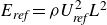 $E_{\textit{ref}}=\rho U_{\textit{ref}}^2L^2$
.
$E_{\textit{ref}}=\rho U_{\textit{ref}}^2L^2$
.
Figure 17 presents the average strain energy, kinetic energy and total mechanical energy of the plate and the blade array as functions of the blade bending stiffness $K_b$
. For the plate, its average strain energy
$K_b$
. For the plate, its average strain energy $\widetilde {E_{s,p}}$
(blue line) is significantly smaller than its average kinetic energy
$\widetilde {E_{s,p}}$
(blue line) is significantly smaller than its average kinetic energy $\widetilde {E_{k,p}}$
(red line), contributing negligibly to the average total mechanical energy
$\widetilde {E_{k,p}}$
(red line), contributing negligibly to the average total mechanical energy $\widetilde {E_{t,p}}$
(black line). As
$\widetilde {E_{t,p}}$
(black line). As $K_b$
increases, both
$K_b$
increases, both $\widetilde {E_{k,p}}$
and
$\widetilde {E_{k,p}}$
and $\widetilde {E_{t,p}}$
first increase rapidly, then decrease to a local minimum, and finally rise gradually. In contrast, for the blade array, its average strain energy
$\widetilde {E_{t,p}}$
first increase rapidly, then decrease to a local minimum, and finally rise gradually. In contrast, for the blade array, its average strain energy $\widetilde {E_{s,b}}$
, average kinetic energy
$\widetilde {E_{s,b}}$
, average kinetic energy $\widetilde {E_{k,b}}$
, and average total mechanical energy
$\widetilde {E_{k,b}}$
, and average total mechanical energy $\widetilde {E_{t,b}}$
exhibit the opposing trend: they initially decrease rapidly, then rise to a local maximum, and finally decay gradually to zero as the blades become increasingly rigid. Resonance occurs when
$\widetilde {E_{t,b}}$
exhibit the opposing trend: they initially decrease rapidly, then rise to a local maximum, and finally decay gradually to zero as the blades become increasingly rigid. Resonance occurs when $\widetilde {E_{t,b}}$
reaches a local maximum, where the corresponding
$\widetilde {E_{t,b}}$
reaches a local maximum, where the corresponding $K_b$
(marked by the black dashed line) is defined as the resonant bending stiffness
$K_b$
(marked by the black dashed line) is defined as the resonant bending stiffness $K_r$
. Furthermore,
$K_r$
. Furthermore, $\widetilde {E_{t,b}}$
is significantly smaller than
$\widetilde {E_{t,b}}$
is significantly smaller than $\widetilde {E_{t,p}}$
, indicating that the energy stored in the blade array accounts for only a small fraction of the total energy in the system.
$\widetilde {E_{t,p}}$
, indicating that the energy stored in the blade array accounts for only a small fraction of the total energy in the system.
The resonance phenomenon is also confirmed from the frequency perspective. Table 3 summarises the dimensionless flapping frequency $f^*$
of the self-propelled plate and the natural frequency
$f^*$
of the self-propelled plate and the natural frequency $f_n^{inv} L/U_{\textit{ref}}$
of the blades. Here,
$f_n^{inv} L/U_{\textit{ref}}$
of the blades. Here, $f_n^{inv}$
is calculated through (3.17) by setting the dimensionless bending stiffness to
$f_n^{inv}$
is calculated through (3.17) by setting the dimensionless bending stiffness to $K_r$
. In all cases,
$K_r$
. In all cases, $f^*$
is close to but approximately 20 % lower than
$f^*$
is close to but approximately 20 % lower than $f_n^{inv} L/U_{\textit{ref}}$
, a phenomenon also documented in the work of Xiong et al. (Reference Xiong, Gao, Lu and Chen2024). This is because the resonance frequency of a strongly damped system is lower than its natural frequency without damping, as illustrated in the vibration theory (Rao Reference Rao2010).
$f_n^{inv} L/U_{\textit{ref}}$
, a phenomenon also documented in the work of Xiong et al. (Reference Xiong, Gao, Lu and Chen2024). This is because the resonance frequency of a strongly damped system is lower than its natural frequency without damping, as illustrated in the vibration theory (Rao Reference Rao2010).
The dimensionless flapping frequency $f^*$
and the natural frequency
$f^*$
and the natural frequency $f_n^{inv} L/U_{\textit{ref}}$
of the compliant blades when resonance occurs.
$f_n^{inv} L/U_{\textit{ref}}$
of the compliant blades when resonance occurs.

Table 3. Long description
The table presents a comparison between the dimensionless flapping frequency and the natural frequency of compliant blades when resonance occurs. It consists of two rows and three columns. The first row contains the headers ‘f*’ and three numerical values: 0.38, 0.51, and 0.64. The second row is labeled ‘f_n^inv L/U_ref’ and lists the values 0.50, 0.66, and 0.78. The data indicates that the dimensionless flapping frequency is consistently lower than the natural frequency, approximately 20 percent lower, which aligns with findings from previous studies. This discrepancy is attributed to the damping effects in the system, as explained by vibration theory.
The average propulsive velocity $\widetilde {U}$
of the self-propelled plate, and average mechanical energy
$\widetilde {U}$
of the self-propelled plate, and average mechanical energy $\widetilde {E_{t,b}}$
of the compliant blade array, as functions of the blade bending stiffness
$\widetilde {E_{t,b}}$
of the compliant blade array, as functions of the blade bending stiffness $K_b$
, for
$K_b$
, for $(a)\,f^*=0.38$
,
$(a)\,f^*=0.38$
, $(b)\,f^*=0.51$
,
$(b)\,f^*=0.51$
, $(c)\,f^*=0.64$
. Here,
$(c)\,f^*=0.64$
. Here, $A_L=0.5, H_L=1.5, D_L=0.5, K_p=3.5$
. The red dashed lines mark the resonance stiffness
$A_L=0.5, H_L=1.5, D_L=0.5, K_p=3.5$
. The red dashed lines mark the resonance stiffness $K_r$
. The black dashed lines represent
$K_r$
. The black dashed lines represent $\widetilde {U}$
of the corresponding cases without blades.
$\widetilde {U}$
of the corresponding cases without blades.

Figure 18. Long description
The image contains three line graphs labeled (a), (b), and (c). Each graph shows two data series: the average propulsive velocity of the self-propelled plate (black line with square markers) and the average mechanical energy of the compliant blade array (red line with circle markers). The x-axis represents the blade bending stiffness, while the y-axes represent the normalized propulsive velocity and mechanical energy. The red dashed lines mark the resonance stiffness, and the black dashed lines represent the corresponding cases without blades. In all three graphs, the propulsive velocity remains relatively stable, while the mechanical energy decreases as the blade bending stiffness increases. The graphs illustrate how the presence of blades affects the propulsive velocity and mechanical energy of the system.
The spatiotemporal distribution of the total mechanical energy $E_{t, bi}$
of the compliant blades, with bending stiffnesses
$E_{t, bi}$
of the compliant blades, with bending stiffnesses $(a)$
$(a)$ $K_b=1.5$
,
$K_b=1.5$
, $(b)$
$(b)$ $K_b=2.5$
(resonance bending stiffness),
$K_b=2.5$
(resonance bending stiffness), $(c)$
$(c)$ $K_b=10$
. The energy proportions of the three regimes (A, B and C) are marked in the figures. Here,
$K_b=10$
. The energy proportions of the three regimes (A, B and C) are marked in the figures. Here, $f^*=0.51, A_L=0.5, D_L=0.5, H_L=1.5, K_p=3.5$
.
$f^*=0.51, A_L=0.5, D_L=0.5, H_L=1.5, K_p=3.5$
.

Figure 19. Long description
Three graphs illustrate the spatiotemporal distribution of the total mechanical energy of compliant blades with varying bending stiffnesses. Each graph is divided into three regimes labeled A, B, and C, with their respective energy proportions marked. The x-axis represents the normalized position, while the y-axis represents the normalized time. The color gradient indicates the energy levels, with darker shades representing higher energy. The dashed lines in each graph denote specific boundaries or transitions between the regimes. Regime A occupies 1.4 percent, 1.0 percent, and 2.6 percent of the total energy in the three graphs respectively. Regime B occupies 54.2 percent, 42.1 percent, and 77.9 percent. Regime C occupies 44.4 percent, 56.9 percent, and 19.5 percent. The graphs show how the energy distribution changes over time and space for different bending stiffnesses.
Figure 18 presents the average propulsive velocity $\widetilde {U}$
of the self-propelled plate, and average total mechanical energy
$\widetilde {U}$
of the self-propelled plate, and average total mechanical energy $\widetilde {E_{t,b}}$
of the blade array, as functions of the blade bending stiffness
$\widetilde {E_{t,b}}$
of the blade array, as functions of the blade bending stiffness $K_b$
. The black dashed lines denote
$K_b$
. The black dashed lines denote $\widetilde {U}$
for the corresponding cases without blades, and each of them lies below that for the blade-covered wall. Since the magnitudes of
$\widetilde {U}$
for the corresponding cases without blades, and each of them lies below that for the blade-covered wall. Since the magnitudes of $\widetilde {U}$
and
$\widetilde {U}$
and $\widetilde {E_{t,b}}$
differ dramatically across the three frequencies, different
$\widetilde {E_{t,b}}$
differ dramatically across the three frequencies, different $y$
-axis ranges are adopted in each subplot to better visualise the respective trends. The variation of
$y$
-axis ranges are adopted in each subplot to better visualise the respective trends. The variation of $\widetilde {U}$
with
$\widetilde {U}$
with $K_b$
exhibits a negative correlation with that of
$K_b$
exhibits a negative correlation with that of $\widetilde {E_{t,b}}$
, i.e.
$\widetilde {E_{t,b}}$
, i.e. $\widetilde {U}$
first increases rapidly, then decreases to a local minimum, and finally rises gradually with increasing
$\widetilde {U}$
first increases rapidly, then decreases to a local minimum, and finally rises gradually with increasing $K_b$
. As the flapping frequency
$K_b$
. As the flapping frequency $f^*$
of the plate increases, although both
$f^*$
of the plate increases, although both $\widetilde {U}$
and
$\widetilde {U}$
and $\widetilde {E_{t,b}}$
increase, the local minimum of
$\widetilde {E_{t,b}}$
increase, the local minimum of $\widetilde {U}$
and local maximum of
$\widetilde {U}$
and local maximum of $\widetilde {E_{t,b}}$
are flattened, and the resonant bending stiffness
$\widetilde {E_{t,b}}$
are flattened, and the resonant bending stiffness $K_r$
(marked by red dashed lines) increases. Furthermore, at
$K_r$
(marked by red dashed lines) increases. Furthermore, at $f^*=0.38$
, the local minimum of
$f^*=0.38$
, the local minimum of $\widetilde {U}$
nearly coincides with the resonant stiffness
$\widetilde {U}$
nearly coincides with the resonant stiffness $K_r$
; at higher flapping frequencies (
$K_r$
; at higher flapping frequencies ( $f^*=0.51$
and 0.64),
$f^*=0.51$
and 0.64), $\widetilde {U}$
reaches a local minimum at a higher
$\widetilde {U}$
reaches a local minimum at a higher $K_b$
than
$K_b$
than $K_r$
.
$K_r$
.
The dimensionless (a,b,c) vorticity field and (d,e,f) $Q$
field (
$Q$
field (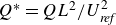 $Q^*=QL^2/U_{\textit{ref}}^2$
) at
$Q^*=QL^2/U_{\textit{ref}}^2$
) at $t/T=19.25$
for different blade bending stiffness values: (a,d)
$t/T=19.25$
for different blade bending stiffness values: (a,d) $K_b=1.5$
, (b,e)
$K_b=1.5$
, (b,e) $K_b=2.5$
(resonance bending stiffness), (c,f)
$K_b=2.5$
(resonance bending stiffness), (c,f) $K_b=10$
. Here,
$K_b=10$
. Here, $f^*=0.51, A_L=0.5, H_L=1.5, D_L=0.5, K_p=3.5$
.
$f^*=0.51, A_L=0.5, H_L=1.5, D_L=0.5, K_p=3.5$
.

Figure 20. Long description
A heat map displays the vorticity field and field values for different blade bending stiffness values near a flat wall. The map is divided into six subplots, with the left column showing vorticity fields and the right column showing field values. Each row corresponds to a different blade bending stiffness value: low, resonance, and high. The vorticity field subplots (a, b, c) use a color scale ranging from blue to red, indicating negative to positive vorticity values. The field value subplots (d, e, f) use a color scale ranging from blue to red, indicating lower to higher field values. The subplots reveal distinct patterns and vortex formations, with notable differences in vortex structures and intensities across the different stiffness values. The presence of downstream tip vortices is highlighted in subplot (e). The overall trend shows variations in vortex interactions and field distributions as the blade bending stiffness changes.
Figure 19 presents the spatiotemporal distribution of the total mechanical energy $E_{t, bi}$
of individual compliant blades at
$E_{t, bi}$
of individual compliant blades at $f^*=0.51$
for three bending stiffnesses:
$f^*=0.51$
for three bending stiffnesses: $K_b=1.5$
,
$K_b=1.5$
, $K_b=K_r=2.5$
and
$K_b=K_r=2.5$
and $K_b=10$
. Being consistent with figure 12, the boundaries of the three regimes A, B and C are marked by black dashed lines. The results indicate that the total mechanical energy of blades in regimes B and C accounts for nearly the entire energy of the blade array. However, their respective proportions vary with
$K_b=10$
. Being consistent with figure 12, the boundaries of the three regimes A, B and C are marked by black dashed lines. The results indicate that the total mechanical energy of blades in regimes B and C accounts for nearly the entire energy of the blade array. However, their respective proportions vary with $K_b$
. For the blade with
$K_b$
. For the blade with $K_b=1.5$
(softer than the resonant bending stiffness
$K_b=1.5$
(softer than the resonant bending stiffness $K_r$
), 54.2 % of the total mechanical energy is distributed in regime B, exceeding that (44.4 %) distributed in regime C. At the resonant stiffness
$K_r$
), 54.2 % of the total mechanical energy is distributed in regime B, exceeding that (44.4 %) distributed in regime C. At the resonant stiffness $K_b=K_r=2.5$
, a larger proportion of energy (56.9 %) is distributed in regime C, because the blades undergo more intense excitation and thus store more mechanical energy. For the stiffer blades with
$K_b=K_r=2.5$
, a larger proportion of energy (56.9 %) is distributed in regime C, because the blades undergo more intense excitation and thus store more mechanical energy. For the stiffer blades with $K_b=10$
, the energy is primarily concentrated in regime B, which accounts for
$K_b=10$
, the energy is primarily concentrated in regime B, which accounts for $77.9\,\%$
of the total energy. These results demonstrate that resonance facilitates energy storage in downstream regions.
$77.9\,\%$
of the total energy. These results demonstrate that resonance facilitates energy storage in downstream regions.
Figure 20 presents distributions of the vorticity and the second invariant of the velocity gradient tensor $Q$
at
$Q$
at $t/T=19.25$
for different blade bending stiffnesses
$t/T=19.25$
for different blade bending stiffnesses $K_b$
. Here, the positive
$K_b$
. Here, the positive $Q$
is also used to indicate concentrated vortices, known as the
$Q$
is also used to indicate concentrated vortices, known as the $Q$
-criterion (Hunt, Wray & Moin Reference Hunt, Wray and Moin1988). Upstream of the leading edge and beneath the plate, the blades are deflected leftwards due to the high-pressure region between the plate and the bottom wall, resulting in the shedding of concentrated positive vortices from the blade tips. As
$Q$
-criterion (Hunt, Wray & Moin Reference Hunt, Wray and Moin1988). Upstream of the leading edge and beneath the plate, the blades are deflected leftwards due to the high-pressure region between the plate and the bottom wall, resulting in the shedding of concentrated positive vortices from the blade tips. As $K_b$
increases, the horizontal displacement of the blade tips decreases progressively; however, the strength of the tip vortices increases. Beneath the trailing-edge vortex and its feeding shear layer, negative vortices are formed at the blade tips. For the resonant case with
$K_b$
increases, the horizontal displacement of the blade tips decreases progressively; however, the strength of the tip vortices increases. Beneath the trailing-edge vortex and its feeding shear layer, negative vortices are formed at the blade tips. For the resonant case with $K_b=K_r=2.5$
, concentrated tip vortices are observed beyond
$K_b=K_r=2.5$
, concentrated tip vortices are observed beyond $2L$
downstream of the plate, confirming that resonance facilitates the vibration of blades in the wake.
$2L$
downstream of the plate, confirming that resonance facilitates the vibration of blades in the wake.
4. Conclusion
A numerical investigation is conducted on a self-propelled flexible plate moving above an array of wall-mounted compliant blades, designed to mimic flatfish-like locomotion near a vegetation-covered seabed. This work focuses on two core aspects: the propulsive performance of the plate, and the forced vibration responses of the blade array. The effects of key dimensionless parameters, including the flapping frequency $f^*$
of the plate, blade spacing
$f^*$
of the plate, blade spacing $D_L$
, vertical distance between the plate and bottom wall
$D_L$
, vertical distance between the plate and bottom wall $H_L$
, and bending stiffness
$H_L$
, and bending stiffness $K_b$
of the blades, are systematically investigated.
$K_b$
of the blades, are systematically investigated.
This reveals that the blade array suppresses the deformation of the self-propelled plate while enhancing its propulsive performance, as evidenced by an increase in propulsive velocity and a reduction in cost of transport ( ${\textit{COT}}$
). Such enhancement becomes more pronounced as
${\textit{COT}}$
). Such enhancement becomes more pronounced as $D_L$
and
$D_L$
and $H_L$
decrease, before direct solid–solid contact occurs. Moreover, an increase in flapping frequency of the plate
$H_L$
decrease, before direct solid–solid contact occurs. Moreover, an increase in flapping frequency of the plate $f^*$
enhances its propulsive velocity at the expense of higher energy consumption. Furthermore, by introducing a correction factor to account for the asymmetric motion of the plate during the upper and lower half-periods, a universal scaling law
$f^*$
enhances its propulsive velocity at the expense of higher energy consumption. Furthermore, by introducing a correction factor to account for the asymmetric motion of the plate during the upper and lower half-periods, a universal scaling law ${\textit{Re}}_c\sim ({\textit{Re}}_{f,\delta })^{3/2}$
is identified between the propulsive Reynolds number
${\textit{Re}}_c\sim ({\textit{Re}}_{f,\delta })^{3/2}$
is identified between the propulsive Reynolds number ${\textit{Re}}_c$
and the corrected flapping Reynolds number
${\textit{Re}}_c$
and the corrected flapping Reynolds number ${\textit{Re}}_{f,\delta }$
.
${\textit{Re}}_{f,\delta }$
.
Based on the spatiotemporal diagrams of the blade-tip displacements, three distinct regimes are identified within the blade array. Regime A covers blades upstream of the plate’s leading edge, which exhibit negligible vibrations except in the immediate vicinity of the leading edge. Regime B includes blades that are directly excited by the plate over one period, and these blades form a flapping-driven vibration region synchronised with the plate’s motion. Regime C consists of downstream blades undergoing underdamped free vibration, where a series of FPTWs arises. These waves are strongly correlated with the pressure distribution within the blade array, and originate from the cooperative underdamped vibration of downstream blades.
Resonance occurs between the flapping plate and the blade array when the flapping frequency of the plate approaches the natural frequency of the blades. At resonance, the blade array absorbs more energy from the system, resulting in a local maximum in its total mechanical energy. Conversely, the propulsive velocity of the plate exhibits a local minimum, which remains higher than that in the corresponding case without blades.
This study yields several implications. First, for underwater swimmers, it is beneficial to leverage the bottom wall to achieve higher propulsive performance, while resonance with surrounding elastic structures should be avoided. Second, the dynamic responses of compliant structures serve as robust indicators of nearby swimmers, offering substantial potential for applications in flow-sensing technologies. Nevertheless, the present investigation is restricted to relatively low Reynolds numbers, and the propulsive performance of near-bottom swimmers at higher Reynolds numbers remains to be systematically explored in future work.
Supplementary movies
Supplementary movies are available at https://doi.org/10.1017/jfm.2026.11712.
Acknowledgements
We thank the University of Science and Technology of China Supercomputing Centre for providing computational resources for this project.
Funding
This work is supported by the National Natural Science Foundation of China (grant nos 12302320, 12388101, 12293000 and 12293002).
Declaration of interests
The authors report no conflict of interest.
Data availability statement
The data that support the findings of this study are available from the corresponding author upon reasonable request.
Appendix A. Dimensionless governing equations and boundary conditions
The dimensionless vertical position of the leading edge of the self-propelled plate is given by
 \begin{equation} y_l^*(t^*)= 0.5A_L \sin {(2 \pi f^* t^*+\pi )} + H_L. \end{equation}
The dimensionless incompressible Navier–Stokes equations and the continuity equation are
 \begin{align} \frac {\partial \boldsymbol{u}^*}{\partial t^*} + \boldsymbol{u}^*\boldsymbol{\cdot }\boldsymbol{\nabla }^*\boldsymbol{u}^* &= -\boldsymbol{\nabla }^* p^*+\frac {1}{100}{\nabla} ^{*2} \boldsymbol{u}^*+\boldsymbol{f}_{\textit{IB}}^*, \end{align}
 \begin{align} \boldsymbol{\nabla }^* \boldsymbol{\cdot }\boldsymbol{u}^* &= 0. \\[10pt] \nonumber \end{align}
The dimensionless time, velocity, pressure and volume force are defined as
 \begin{equation} t^*=\frac {tU_{\textit{ref}}}{L},\quad \boldsymbol{u}^*=\frac {\boldsymbol{u}}{U_{\textit{ref}}},\quad p^*=\frac {p}{\rho U_{\textit{ref}}^2},\quad \boldsymbol{f}_{\textit{IB}}^*=\frac {L\boldsymbol{f}_{\textit{IB}}}{\rho U_{\textit{ref}}^2}. \end{equation}
The dimensionless governing equation for the beam is given by
 \begin{equation} \rho ^*\frac {\partial ^2\boldsymbol{X}^*}{\partial t^{*2}} - S\frac {\partial }{\partial s^*}\left [\left (1-\left |\frac {\partial \boldsymbol{X}^*}{\partial s^*}\right |^{-1}\right )\frac {\partial \boldsymbol{X}^*}{\partial s^*}\right ] + K\frac {\partial ^4 \boldsymbol{X}^*}{\partial s^{*4}} = \boldsymbol{F}_{\textit{IB}}^*. \end{equation}
The boundary condition at the leading edge of the self-propelled plate is given by
 \begin{equation} \left .\frac {\partial X_p^*}{\partial s^*}\right |_{s^*=0} = 1,\quad \left .\frac {\partial Y_p^*}{\partial s^*}\right |_{s^*=0} = 0,\quad Y_p^*(0,t^*) = y_l^*(t^*). \end{equation}
Meanwhile, the boundary conditions at the root of the $i$
th blade are given by
$i$
th blade are given by
 \begin{equation} \left .\frac {\partial X_{\textit{bi}}^*}{\partial s^*}\right |_{s^*=0} = 0,\quad \left .\frac {\partial Y_{\textit{bi}}^*}{\partial s^*}\right |_{s^*=0} = 1,\quad X_{\textit{bi}}^*(0,t^*) = -iD_L , \quad Y_{\textit{bi}}^*(0,t^*) = 0. \end{equation}
At the free ends of the plate and blades, the following boundary conditions are applied:
 \begin{equation} \left [S\left (1-{\left |\frac {\partial \boldsymbol{X}^*}{\partial s^*}\right |}^{-1}\right )\frac {\partial \boldsymbol{X}^*}{\partial s^*} - K\frac {\partial ^3\boldsymbol{X}^*}{\partial s^{*3}}\right ]_{s^*=1} = \boldsymbol{0}, \quad \left .\frac {\partial ^2\boldsymbol{X}^*}{\partial s^{*2}}\right |_{s^*=1} = \boldsymbol{0}. \end{equation}
The dimensionless position vector and external force are defined as
 \begin{equation} \boldsymbol{X}^*=\frac {\boldsymbol{X}}{L},\quad s^*=\frac {s}{L},\quad \boldsymbol{F}_{\textit{IB}}^*=\frac {\boldsymbol{F}_{\textit{IB}}}{\rho U_{\textit{ref}}^2}. \end{equation}
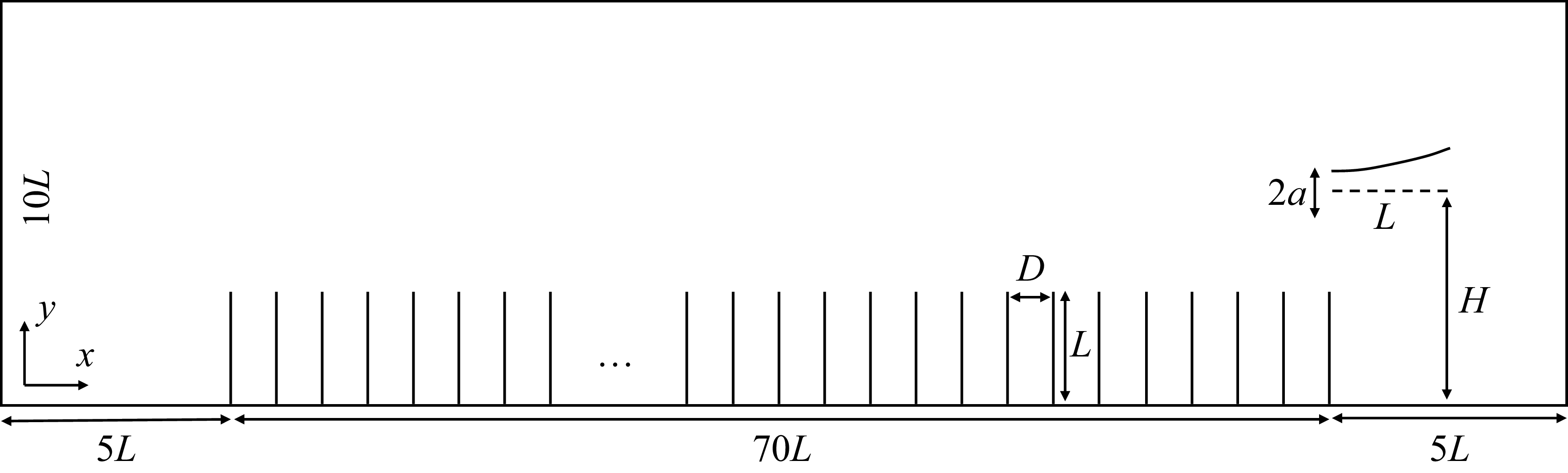

 (a)
(a) (b)
(b)

 t/T=19.75
 (a)
(a) (DL→∞,HL→∞)
 (b)
(b) (DL→∞,HL=1.5)
 (c)
(c) DL=1.00,HL=1.5
 (d)
(d) DL=0.50,HL=1.5
 (e)
(e) DL=0.25,HL=1.5
 (f)
(f) DL→∞,HL=0.5
 f∗=0.64,AL=0.5,Kp=3.5,Kb=3.0
 (a)
(a) yl
yl yt
yt t1=19.14T
 t2=19.64T
 (b)
(b) Fx
Fx t3=19.44T
 DL=0.25
 f∗=0.64,AL=0.5,HL=1.5,Kp=3.5,Kb=3.0
 t1=19.14T
 t3=19.44T
 DL→∞,HL=1.5
 DL=0.25
 HL=1.5
 f∗=0.64,AL=0.5,Kp=3.5,Kb=3.0
 (a)
(a) (b)
(b) t1
t1 t2
t2 f∗=0.64,AL=0.5,Kp=3.5,Kb=3.0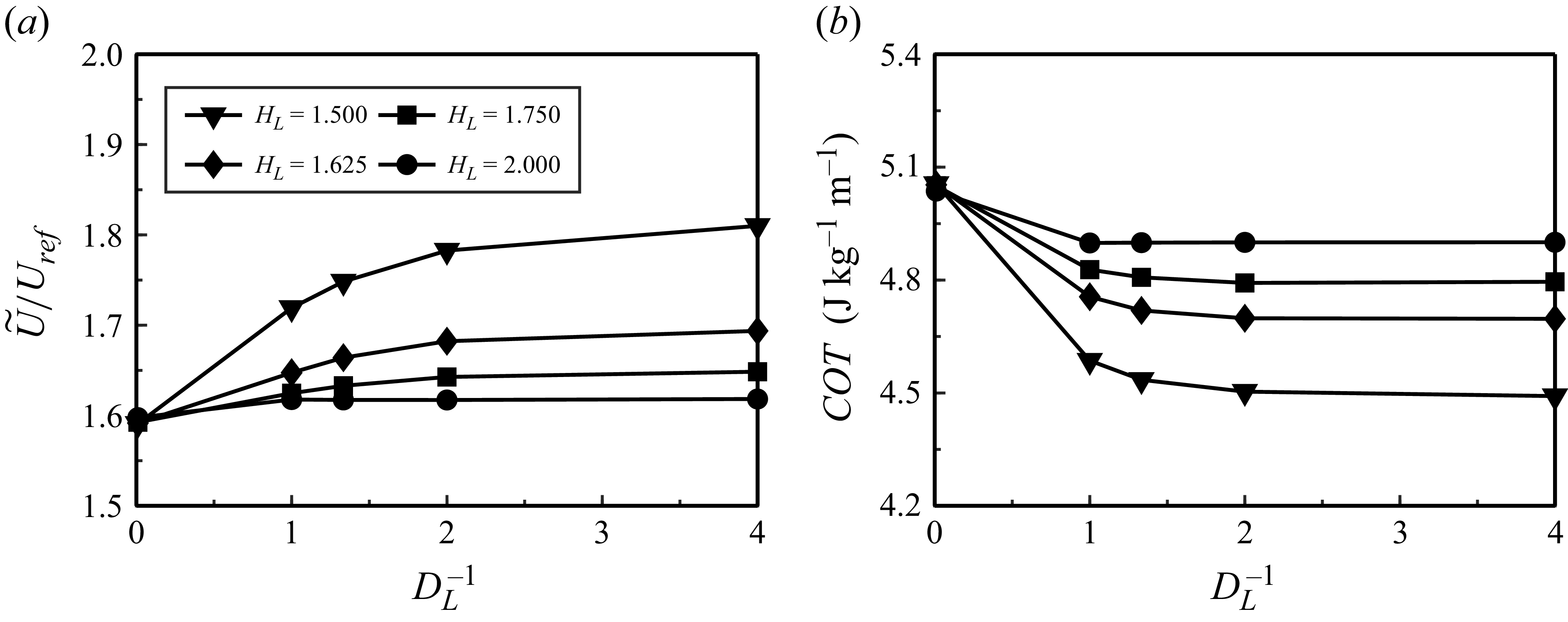
 (a)
(a) (b)
(b) DL−1
DL−1 HL
HL f∗=0.64,AL=0.5,Kp=3.5,Kb=3.0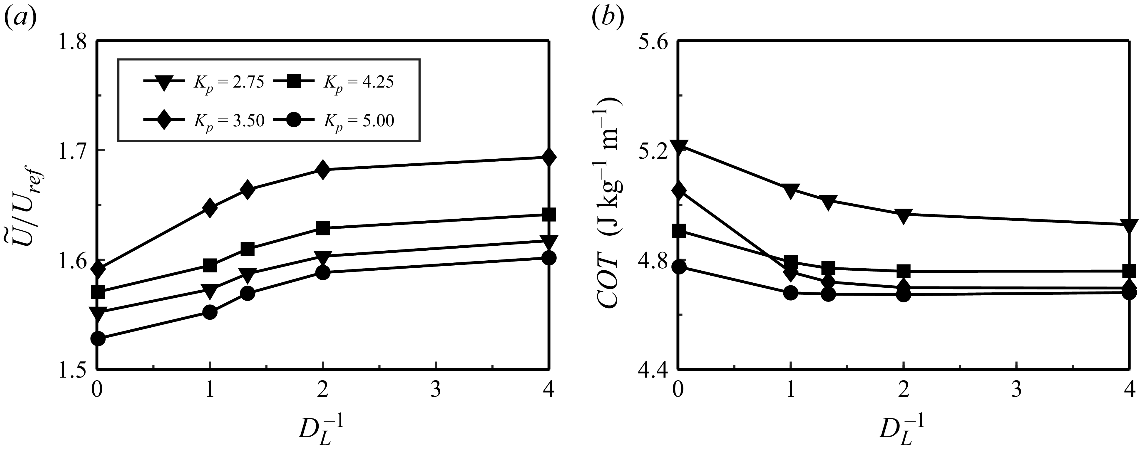
 (a)
(a) (b)
(b) DL−1
DL−1 Kp
Kp f∗=0.64,AL=0.5,HL=1.625,Kb=3.0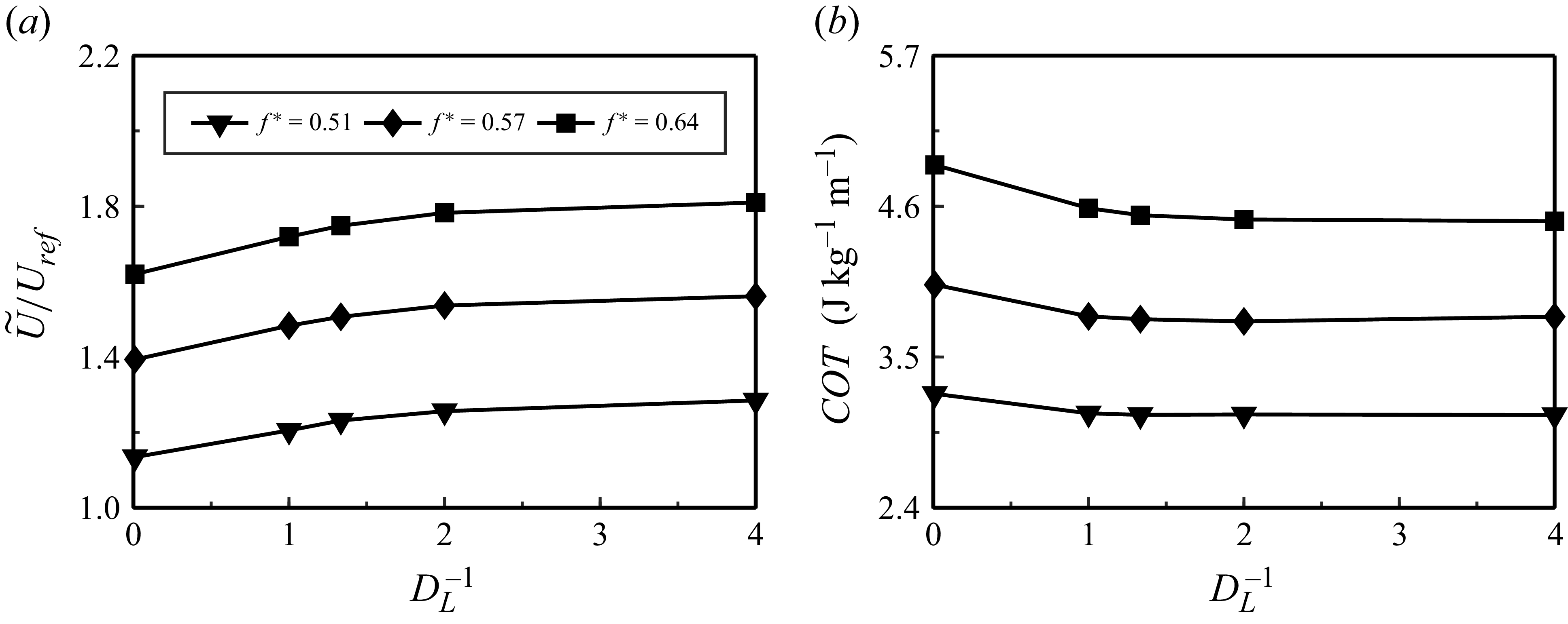
 (a)
(a) (b)
(b) DL−1
DL−1 f∗
f∗ HL=1.5,AL=0.5,Kp=3.5,Kb=3.0
 Rec
Rec Ref
Ref (a)
(a) (b)
(b) f∗=0.64,Kp=3.5,Kb=3.0,0.1⩽AL⩽0.5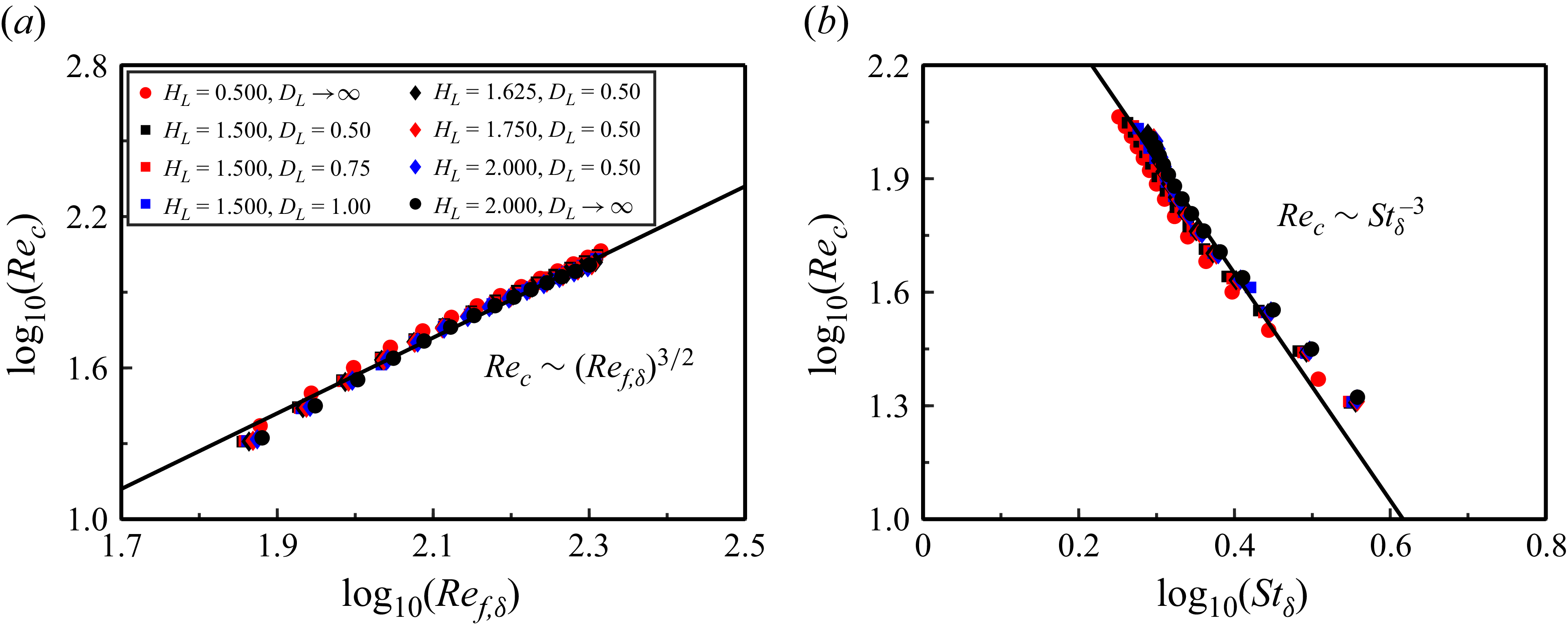
 (a)
(a) Rec
Rec Ref,δ
Ref,δ (b)
(b) Rec
Rec Stδ
Stδ f∗=0.64,Kp=3.5,Kb=3.0,0.1≤AL≤0.5
 dx
dx x
x (a)f∗=0.51
 (b)f∗=0.57
 (c)f∗=0.64
 T
T AL=0.5,DL=0.25,HL=1.5,Kp=3.5,Kb=3.0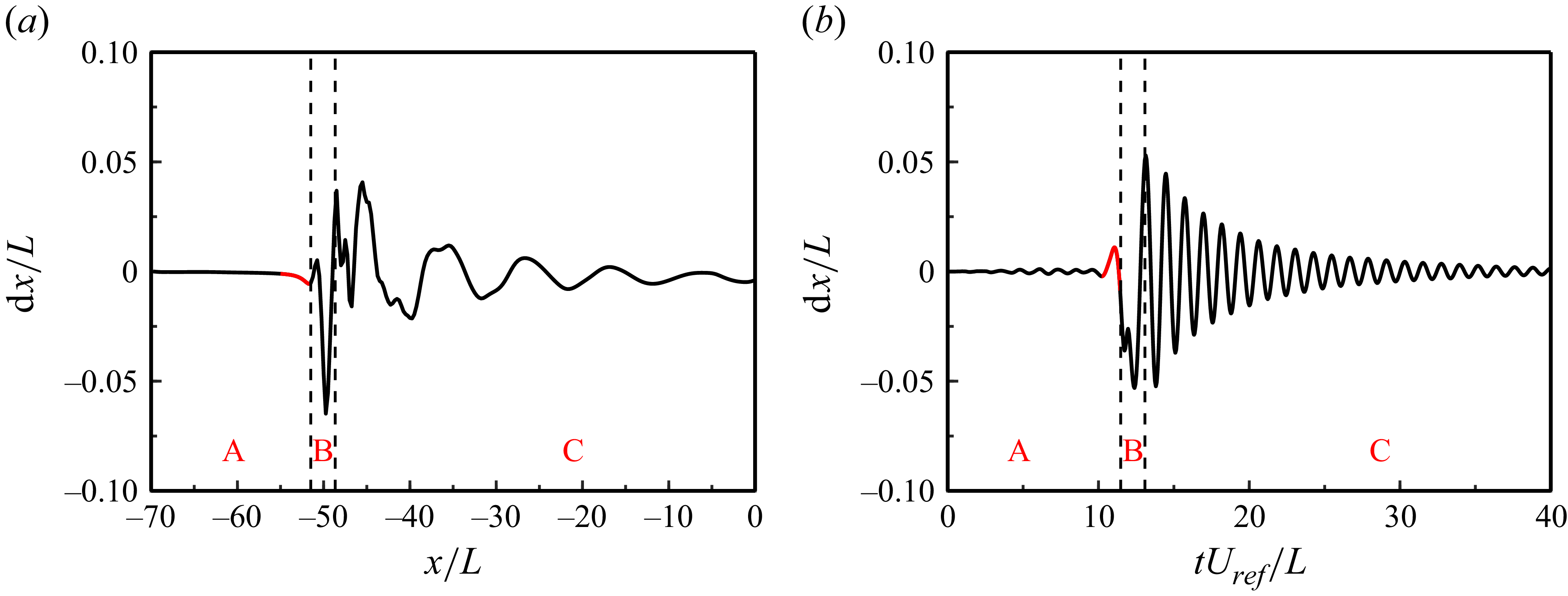
 (a)
(a) t/T=19.00
 (b)
(b) x/L=−17.25
 f∗=0.64,AL=0.5,DL=0.25,HL=1.5,Kp=3.5,Kb=3.0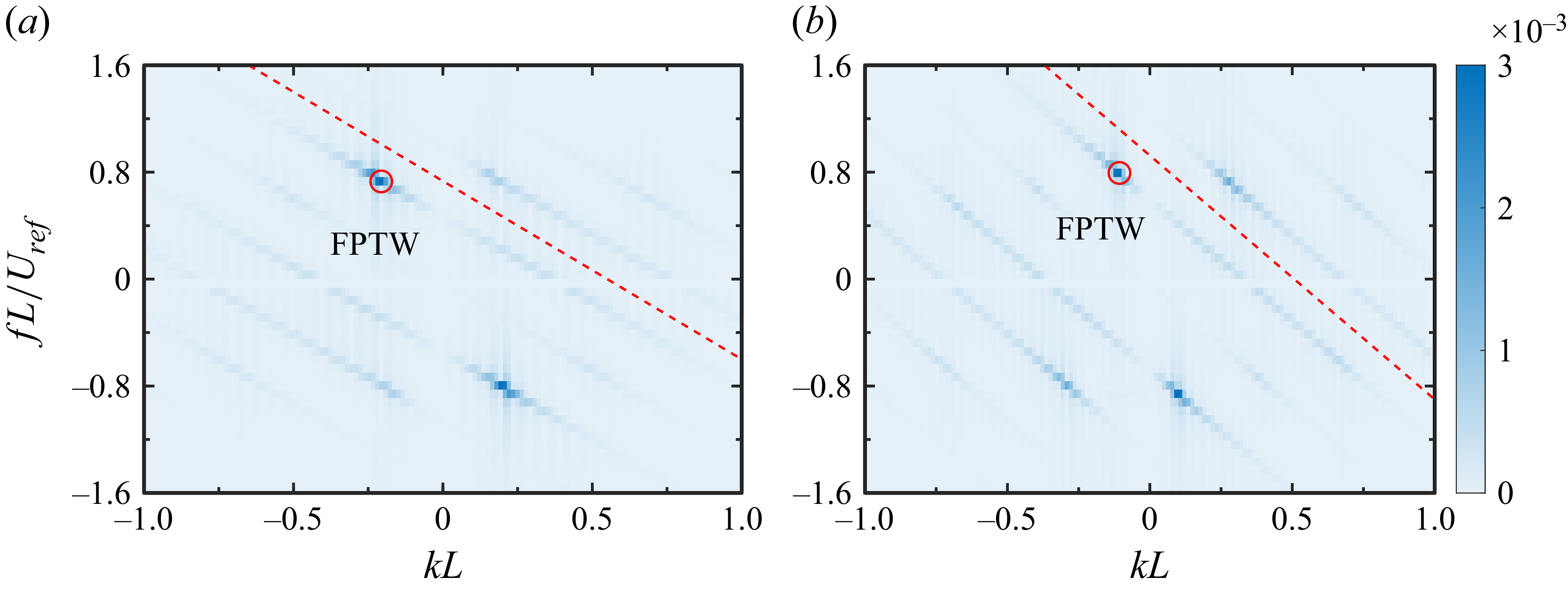
 (a)f∗=0.51
 (b)f∗=0.64
 (Ug=−df/dk)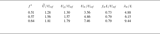
 U~/Uref
 Ug/Uref
 Uw/Uref
 fwL/Uref
 λw/L
λw/L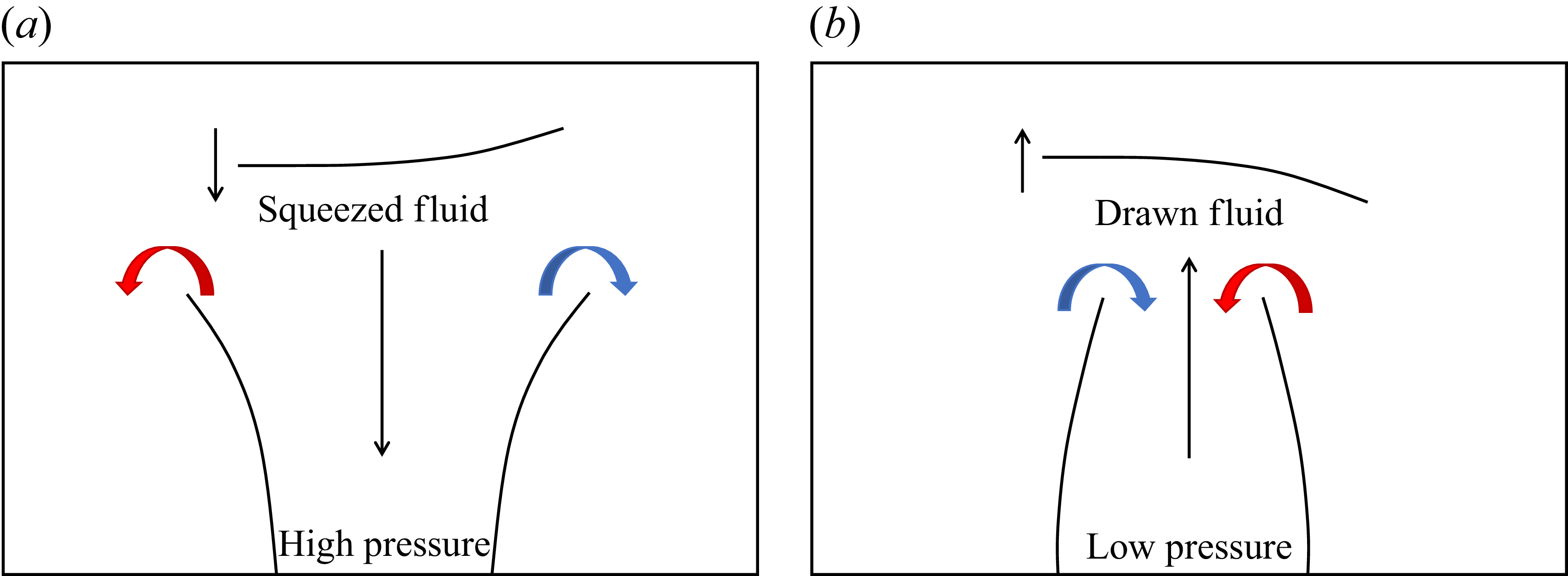
 (a)
(a) (b)
(b)
 t/T=19.00
 (a)f∗=0.51
 (b)f∗=0.57
 (c)f∗=0.64
 λw
λw AL=0.5,HL=1.5,DL=0.25,Kp=3.5,Kb=3.0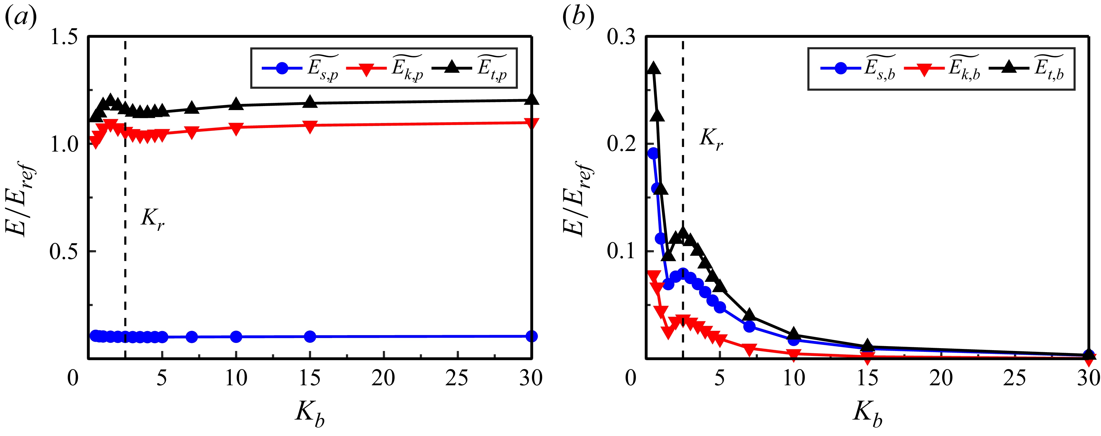
 (a)
(a) (b)
(b) Kb
Kb f∗=0.51,AL=0.5,HL=1.50,DL=0.50,Kp=3.5
 f∗
f∗ fninvL/Uref
 U~
U~ Et,b~
Et,b~ Kb
Kb (a)f∗=0.38
 (b)f∗=0.51
 (c)f∗=0.64
 AL=0.5,HL=1.5,DL=0.5,Kp=3.5
 Kr
Kr U~
U~
 Et,bi
Et,bi (a)
(a) Kb=1.5
 (b)
(b) Kb=2.5
 (c)
(c) Kb=10
Kb=10 f∗=0.51,AL=0.5,DL=0.5,HL=1.5,Kp=3.5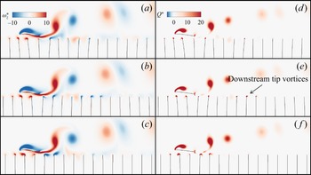
 Q
Q Q∗=QL2/Uref2
 t/T=19.25
 Kb=1.5
 Kb=2.5
 Kb=10
Kb=10 f∗=0.51,AL=0.5,HL=1.5,DL=0.5,Kp=3.5


 Open access

