Database and Measurements

During the 1995 and 1997 Italian Antarctic expeditions, data were collected on the David Glacier-Drygalski Ice Tongue, East Antarctica (Fig. 1). An airborne radio-echo-sounding system flying 300 m above the ice surface with two folded dipole antennas arranged beneath the wings was used. The radio-echo-sounding system operates at 60 MHz with a pulse length switchable between 1 μ and 0.3 μs; the transmitted power, about 1.5 kW, allows an echo signal of adequate amplitude at the input to the receiver. The received echo signal is digitized at a sampling frequency of 20 MHz, so the precision in time detection is 50 ns. In laboratory tests an error Ah of ±8–10 m including a digitizing error due to the poor S/N ratio (<3dB) from the receiver bandwidth of 16 MHz was obtained. The data files show the position and time, obtained from a global-positioning-system (GPS) 4000SSE Trimble receiver interfaced to the radar system. The horizontal sampling rate, at a speed of 200 km h⁻¹, is about 20 traces per kilometre.

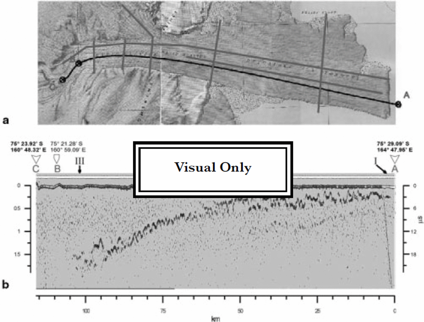
Fig. 1 David-Drygalski glacier: (a) USGS topographic map showing survey flight line, (b) ice thickness vs distance. Two-way time scale is also indicated.

Figure 1 shows one of the longitudinal profiles of the Drygalski ice tongue. By using a radio-wave velocity of 168 m Ms (Reference RobinRobin, 1975; Reference PatersonPaterson, 1981; Reference Bogorodsky, Bentley and GudmandsenBogorodsky and others, 1985), the ice thickness was calculated to range from 150–1500 m. In Figure 2 the whole ice tongue is split into two plots to make the bottom structure more evident. A rippled bottom morphology is clear, showing rather regular waves with a spatial length of about 2 km and a depth variation (peak-to-trough) of about 150–200 m; this feature is also observed on the other two longitudinal profiles.

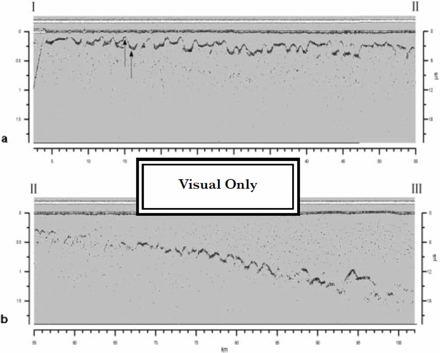
Fig. 2. David-Drygalski glacier. Profile is divided into two parts of about 50 km to make the rippled bottom surface more evident. Arrows in (a) show peak and trough where radar traces (Fig 3a and b) were taken.

Figure 3 shows two radar traces; the first located on the peak of one of the waves of the rippled surface (Fig. 3a) and the second on the trough of the same wave (Fig. 3b).

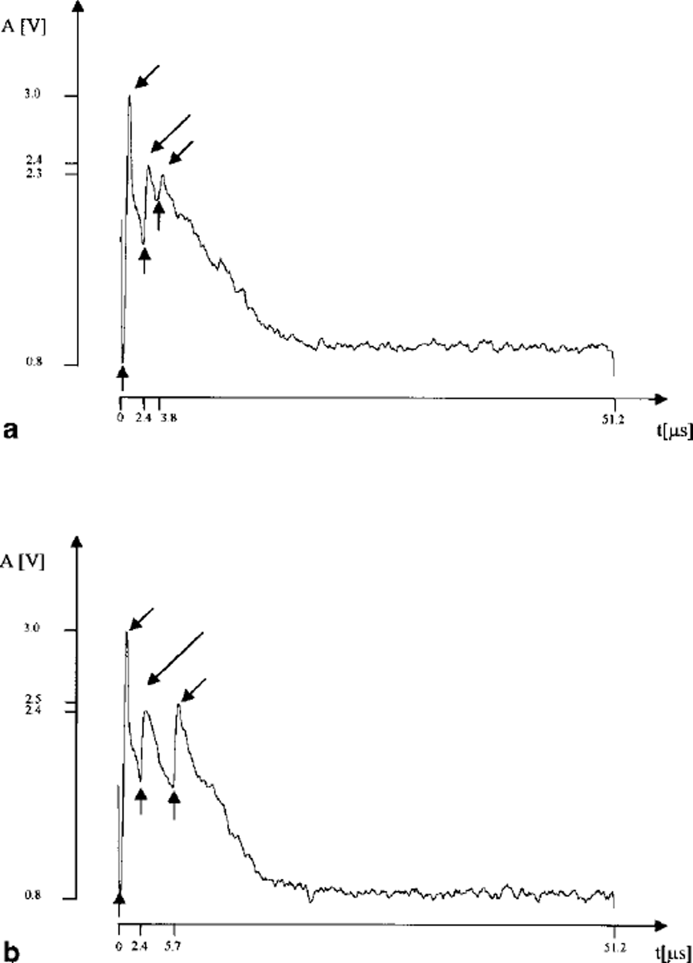
Fig. 3. Examples of radar trace. On the × axis the 51.2 s listening time is indicated as well as relevant arrival times, while on they axis the relative amplitude of the signal is shown in volts. (a) trace from a bottom-surface peak and (b)from a trough. In both examples A₀ is the amplitude of the transmitted peak, A, is the reflection from ice the surface and A₂ the bedrock echo. Mote the different absolute values for A2 amplitude in the bottom reflection of the two plots.

The amplitude of the transmitted pulse, A0, and of the reflected pulse from the ice surface, Ah are the same on both traces, with values of 3.0 V and 2.4 V in a logarithmic scale, respectively. The amplitude, A₂) and the two-way travel time of the bottom reflections, t2, are 2.3 Vand 3.8 Ms in Figure 3a, and 2.5 V and 5.7 μs in Figure 3b. The amplitude of the bottom reflection of Figure 3a is smaller than that in Figure 3b, the difference being about 3.8 dB; if we take into account that the Figure 3a bottom is shallower than the Figure 3b bottom (distance between peak and trough is about 160 m), an apparent contradiction arises: a simple evaluation of geometrical attenuation and ice absorption indicates the deepest reflection is about 9 dB less than the shallowest one. This is observed on all the waves of the bottom topography of the ice tongue up to the grounding line.

The main aim of this paper is to contribute to an explanation of this apparent contradiction.

Radio-Propagation Analysis

We take into account two different hypotheses to try to solve the problem.

The rippled morphology of the ice-tongue bottom was obtained by radar measurements, assuming that the deepest reflections are due to the ice-sea-water interface (Fig. 4a). On the contrary, if we assume that the peak area might be filled by sea ice (Fig. 4b) we would have to consider that the reflections on the peak area were due to the ice-sea-ice interface, and that only the reflections from the trough were due to the ice-sea-water interface.

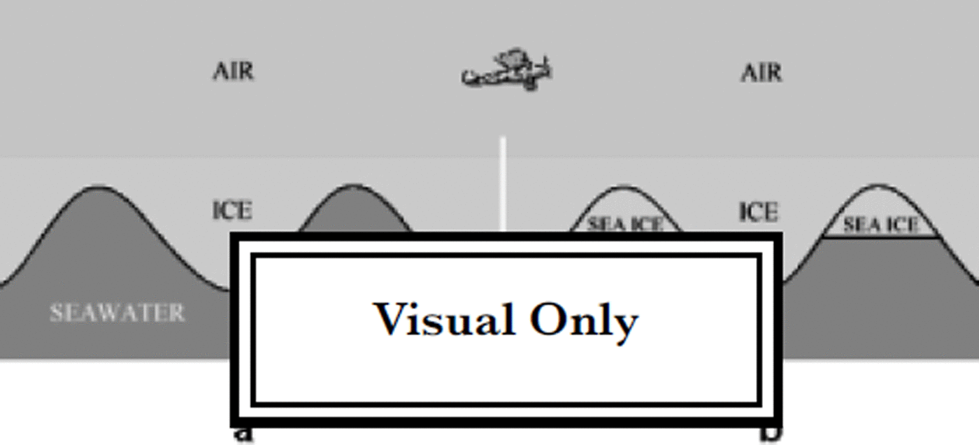
Fig. 4. Possible models describing the different interfaces between the media in an ice tongue.

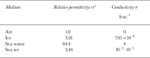
Assuming the ice model in Figure 4b, we could explain the very low reflected energy from the peak area by considering that the relative permittivities of the two media, glacier ice and sea ice, are very similar (Table 1). Moreover, due to the high conductivity of sea ice, the energy is strongly absorbed, making the reflected signal from the sea-ice-sea-water interface almost undetectable. Obviously in this case the calculated ice thicknesses are affected by an error, because of the poor S/N ratio (Reference Bogorodsky, Bentley and GudmandsenBogorodsky and others, 1985). Unfortunately, the low accuracy of the GPS data does not allow an accurate determination of the height above sea level, for calculating the true ice thickness with the floating-ice model.

The second hypothesis is based on the possibility that the ice-sea-water interface is the only one present, so the model in Figure 4a is considered.

An electromagnetic interpretation of echo-signal amplitudes (dynamic analysis) of these profiles has been undertaken to compare the measured amplitudes with the expected ones produced by the characteristic bottom morphology obtained by the kinematic analysis.

The ice-sea-water interface shows concave and convex faces producing a focusing or defocusing effect, detected as a relative amplitude variation in the echo signal. Our purpose is to characterize the propagation of the radio wave through the ice structure by means of a function Lf that includes the gain and loss due to the geometric shape of the reflecting surfaces. Such a function can be evaluated assuming knowledge of the total loss and gain the propagation contributes. In order to evaluate the Lf function let us consider the expression of the received power as

where P_r and P_t are the received and transmitted power, respectively, R is the distance from the reflectors, G the antenna gain, A the wavelength, L and Q represent all the losses and the gains along the path, respectively. Q is the focusing gain due the refractive effect of the ice, depending on the dielectric permittivities air-to-ice ratio and the terrain-clearance to ice-thickness ratio (Reference Bogorodsky, Bentley and GudmandsenBogorodsky and others, 1985).

The loss L can be summarized by Expression (2),

where L_g is geometric loss, L_R and L_T are the reflection and the transmission losses, L_p is the polarization loss due to the orientation of the receiving antenna related to the received radio wave, L_a is the absorption of the ice, L_s is the scattering loss and Lf is the gain or loss of the bottom reflecting surfaces. If we estimate some characteristics of the glacier, such as temperature, chemical composition, surface roughness etc., we can give an approximate value for the electromagnetic constant of the medium at 60–100 MHz (Reference Bogorodsky, Bentley and GudmandsenBogorodsky, 1985; Reference Frolik and YagleFrolik and Yagle, 1995; Reference Henrique and KofmanHenrique and Kofman, 1997). Then the losses due to the propagation velocity can be evaluated easily. The next objective is to determine the single contribution of P_t, P_r L and Q, P_t being a known quantity in our system whose value is about 62 dB m. The received signal power P_r (absolute value) at the receiving-antenna input is evaluated from the voltage amplitude measured at the output of the receiver. This is possible if the transfer function of the log receiver is determined. The answer function of the log receiver is the following:

where A is the measured amplitude of the signal in volts, Vin the amplitude of the signal at the input of the receiver with respect to IV. Obviously Relation (3) is valid only in a range compatible with receiver sensitivity, from –110 dBm to –20dBm. Out of this range Relationship (3) is no longer valid because of electronic saturation. Due to the large bandwidth of the receiver, we can neglect bias caused by the previously reflected signals and antenna ringing. Moreover, the first signal reflected by the ice surface is roughly the same along the whole path; so the systematic error in the amplitude evaluation is partially eliminated in the differences between the first and second reflections.

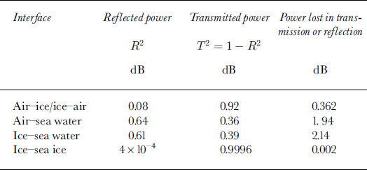
It is possible to know the received signal power, P_T, at the receiving antenna if we determine the real antenna gain from Relation (3). The calibration test performed in the field established that the antenna gain of the folded dipole beneath the reflector was G ≈ 2.5 at the operating frequency of 60 MHz. The trace in Figure 3 allows scaling of the time and amplitude values and calculation of the geometric loss, Lg and attenuation loss, L_a, if we assume the ice conductivity, a. This latter quantity is strictly related to the temperature, T, of the glacier. The dielectric permittivity of the various media also allows calculation of the power lost in the reflection (L_R) and in the transmission process (L_T) at each interface (see Table 2). In Table 2, R and T are the reflection and transmission coefficients. We can summarize all these reflection and transmission loss contributions in a term, L_R–_T which has a value of about 5 dB. The factor (Gλ/4π)2 of Equation (1) can be termed G_A which, in this particular case, has a value of about OdB. Since there is a compensation effect between L_p, Ls and Q we can neglect their contributions thus obtaining the following expression for the function of geometric shape of the reflectors, Lf:

Theoretically, in the case of a flat surface, of homogeneous media and of a perfect calibration, the second member of Relation (4) must be zero. Of course, in evaluating L f it is also assumed that, over the considered horizontal spatial scale, the electromagnetic properties of the media do not change.

But, as already pointed out, this function can be positive or negative depending on the geometrical shape at the ice-sea-water interface, because the vertical section of the concave/convex surface is a parabolic-like reflector and the aircraft is very close to its focus. In this hypothesis, a positive contribution (focusing gain) is expected when there is a concave reflecting surface, while a convex surface gives a negative contribution (defocusing gain). The Lf values compared with the ice thickness are reported in Figures 5 and 6. Lf and the ice thickness show the same trend and periodicity with opposite phase. In particular, where the bottom exhibits large concavities (Fig. 5b, A′ and C′; Fig. 6b, D′ and F′), Lf shows positive peaks (Fig. 5a, A and C; Fig. 6a, D and F); conversely, on the bottom convexities Lf shows negative peaks (Fig. 5b, zone B′; Fig. 5a, zone B). This trend is observed over the whole ice tongue and could confirm the focusing-defocusing effect. The peak and trough where radar traces were obtained are indicated in Figure 5.

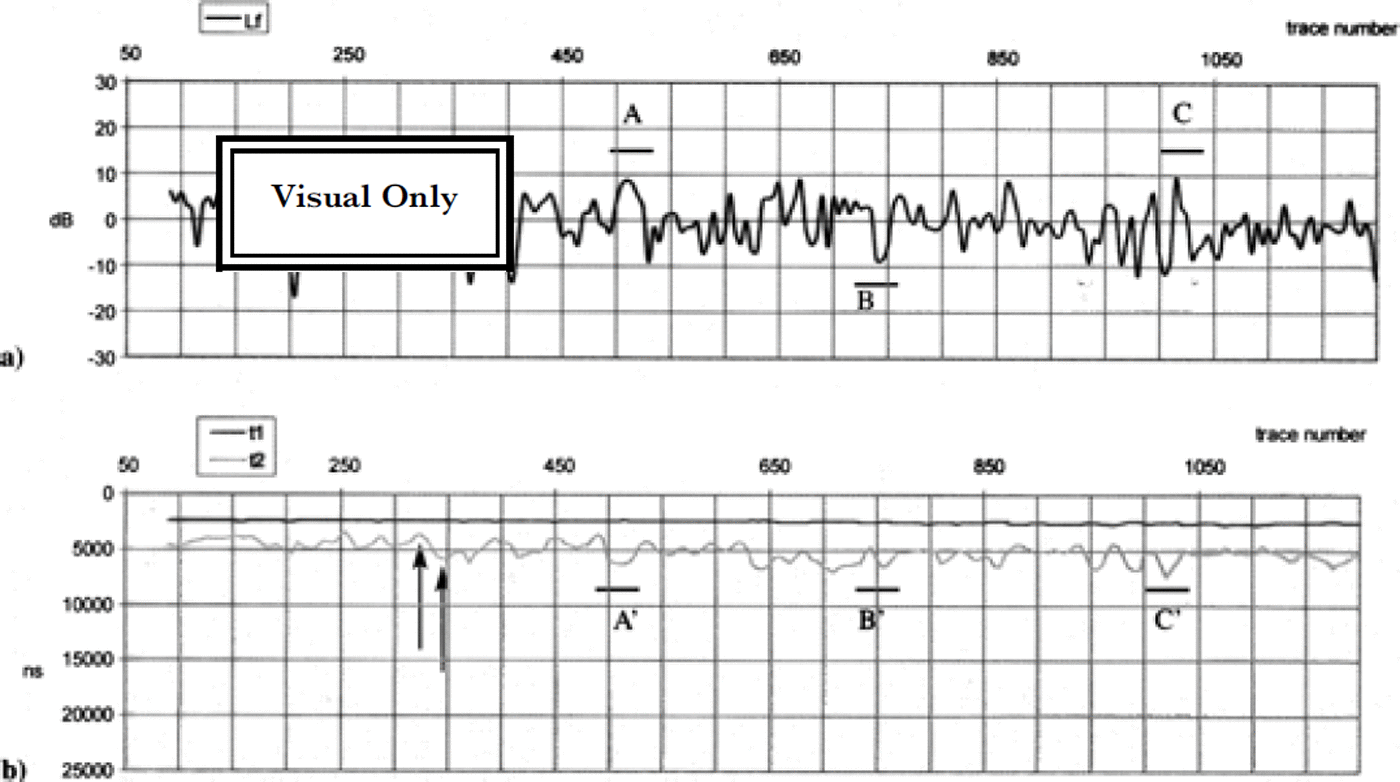
Fig. 5. David-Drygalski glacier profile, first 50 km. (a) Lf function vs trace number; and (b) time delays vs trace number. The very strong positive peaks of Lf correspond to concave reflectors, while the negative peaks coincide with convex surfaces (see letters). Arrows in (b) show peak and trough where radar traces (Fig 3a and b) were taken..

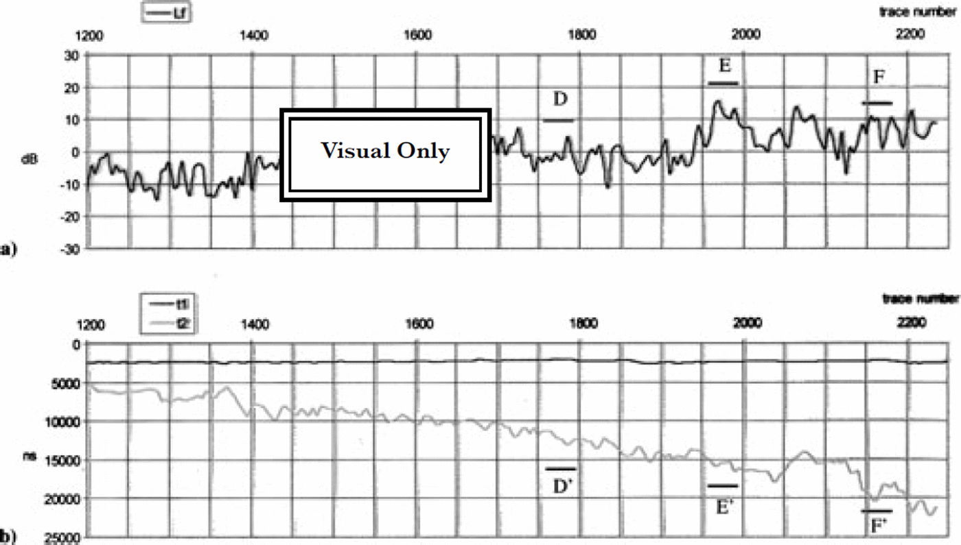
Fig 6. David-Drygalski glacier profile, next 50 km. (a) Lf function vs trace number; and (b) time delays vs trace number.

Near the grounding line, it is not possible to observe the echo signal from the ice-sea-water interface (see Fig. 1), the echo signal from the bottom becomes evanescent and then there is complete loss.

Conclusions

We have presented two different solutions for the apparent contradiction of the amplitudes of the reflections acquired from the peak and trough of the ice bottom.

The first solution, based on the model in Figure 4b, seems to be quite weak because there is no evidence for the presence of sea ice, so the conclusions are only based on a mere hypothesis.

On the contrary, the second solution, taking into account the morphology of the bottom surface of the glacier, seems to be more suitable. It shows that the function Lf has an opposite phase in comparison with the observed bottom rippled surface along the entire ice tongue before the grounding line. Lf depends only on the focusing gain/loss of the reflecting ice-sea-water interface. This confirms that the rippled bottom represents the real morphology of the ice bottom and that the ice thickness and the amplitude of the reflected signals are compatible with the model described in Figure 4a.