


1. Introduction
Owing to the chaotic nonlinear behaviour of its governing equations, which gives rise to data spanning multiple dimensions over a wealth of spatial/temporal scales, turbulence research has pushed the capability of both experiments and numerical simulations to provide large datasets. To reduce the complexity of the information of numerical and experimental datasets, modal analysis based on traditional machine-learning tools such as the proper orthogonal decomposition (known as POD) has been widely exploited in fluid mechanics (Berkooz, Holmes & Lumley Reference Berkooz, Holmes and Lumley1993). Several low-order modelling techniques have flourished, leading to excellent applications to flow understanding and control (Brunton & Noack Reference Brunton and Noack2015; Rowley & Dawson Reference Rowley and Dawson2016).
In recent years, the increasingly powerful tools in machine learning (ML) have led to new approaches for rapidly analysing complex datasets. The main aim is to extract accurate and efficient reduced-order models that capture the essential dynamical features of fluid flows at a reasonable cost (Brunton, Noack & Koumoutsakos Reference Brunton, Noack and Koumoutsakos2020). Machine learning, in general, provides algorithms that process and extract meaningful information from data; they facilitate automation of tasks and augment the underlying knowledge. These techniques are well suited for high-dimensional and nonlinear problems such as those encountered in fluid dynamics. A recent review of model reduction methods for linear systems was done by Benner, Gugercin & Willcox (Reference Benner, Gugercin and Willcox2015), while Brunton & Noack (Reference Brunton and Noack2015) have done a comprehensive overview of ML methods for the control of turbulence.
The increasing availability of high-performance computers is now paving the way to a less explored scenario in fluid mechanics, i.e. using ML to formulate theories. This has the advantage of removing the bias of the researcher, though it requires the right strategy to formulate questions to the computer. An interesting discussion can be found in the work by Jiménez (Reference Jiménez2020), which proposed a ‘Monte Carlo science’ approach grounded on the ever-increasing computational capabilities. The scientific process of formulating the hypothesis is replaced by randomized experiments, evaluated a posteriori. Here we pursue a different approach to mimic our mental process to model the flow behaviour based on looking for patterns in the data. Unsupervised learning is particularly suited for this purpose.
Unsupervised learning is a branch of ML aiming to identify relationships and hidden patterns in the data by specifying certain global criteria and without the need of a supervision or labelling to guide the search (Brunton et al. Reference Brunton, Noack and Koumoutsakos2020). In recent years, we have witnessed the successes of unsupervised ML techniques in different fields of science and engineering containing tasks that need the extraction of features from large-scale experimental or simulation data. For example, in the field of biophysics, which has experienced a substantial expansion in the amount of data generated by atomistic and molecular simulations, in recent years we have witnessed an increased interest in the development and use of algorithms capable of exploiting such data to aid or accelerate scientific discovery. A thorough survey can be found in the work of Glielmo et al. (Reference Glielmo, Husic, Rodriguez, Clementi, Noé and Laio2021), that contains feature representation of molecular systems and presents the state-of-the-art algorithms of dimensionality reduction, density estimation, clustering and kinetic models, implemented in this field. A typical application of unsupervised learning in the field of molecular simulation has been the construction of low-dimensional collective variables to describe a molecular trajectory compactly and effectively.
Among unsupervised-learning techniques, clustering has recently been capturing interest as a tool for the extraction of flow features, which can later form the basis for dynamics modelling and control. For example, the  $K$-means algorithm, the most common clustering approach, has been successfully employed by Kaiser et al. (Reference Kaiser2014a) to develop a data-driven discretization of high-dimensional phase space for the fluid mixing layer. A clustering approach can also be used to partition the reduced-order space of observations into groups to detect similar attributes. Within this clustering arrangement, the flow dynamics can be represented as a linear probabilistic Markov chain (Kaiser et al. Reference Kaiser, Noack, Cordier, Spohn, Segond, Abel, Daviller, Osth, Krajnović and Niven2014b). The Markov-transition dynamics between clusters in the feature space translates to the transition between the flow states associated with the clusters. Such a coarse-graining of the feature space into clusters can be leveraged to systematically incorporate nonlinear control mechanisms (Kaiser et al. Reference Kaiser, Noack, Spohn, Cattafesta and Morzyński2017). In another work, Nair et al. (Reference Nair, Yeh, Kaiser, Noack, Brunton and Taira2019) presented a cluster-based strategy for learning nonlinear feedback control laws directly from coarse-grained fluid flow data. They use cluster analysis in a predefined low-dimensional feature space which is a selection of the aerodynamic forces. The characteristic phase regimes of the flow are then specified by the clusters.
The previously mentioned works have focused on the extraction of reduced-order models of fluid flows profitable for human-supervised physical interpretation, computational optimization and model-based control of flows. Whether artificial intelligence can be used also to identify theories in an unsupervised or weakly supervised manner is an intriguing open question (Jiménez Reference Jiménez2020). The objective of this work is to explore whether ML can help to explain complex fluid-dynamic phenomena with minimal human intervention in the interpretation process. In this study, we address this question through an unsupervised-learning perspective in the context of the boundary layer transition, whose mechanism has been widely investigated and solid theories exist to model it. Here, as will be discussed in the next sections, a local approach is examined to analyse the streamwise evolution of a transitional flow. This local approach is considered to acquire the observations and track them along the flow direction, and is supposed to be more powerful in modelling this type of problem in which there is no periodic behaviour of the flow, while the evolution and the evolving flow is of interest. The present methodology is of course aimed at the analysis of streamwise evolving flows, including transitional flows, shear flows, etc. and does not require an invariance in the spanwise direction.
Transition to turbulence has important practical implications due to the enhanced mixing of momentum, higher skin-friction drag, and heat-transfer rates associated with the onset of turbulence (Kachanov Reference Kachanov1994; Schlichting & Gersten Reference Schlichting and Gersten2017). The interested reader can refer to insightful reviews on the topic of transition to turbulence in boundary layers (Smith Reference Smith1993; Kachanov Reference Kachanov1994; Durbin Reference Durbin2017).
Here, we focus on zero-pressure-gradient boundary layers, where the transition to turbulence is usually classified as orderly or bypass (Zaki Reference Zaki2013). The orderly transition route starts with the amplification of discrete Tollmien–Schlichting instability wave, proceeds through secondary instability and ends with turbulent spots forming locally at the tips of  $\varLambda$ vortices. Bypass transition, on the other hand, is triggered by streaks and follows a different route (e.g. Jacobs & Durbin Reference Jacobs and Durbin2001; Durbin & Wu Reference Durbin and Wu2007; Schlatter et al. Reference Schlatter, Brandt, de Lange and Henningson2008). For additional references see the book by Schmid & Henningson (Reference Schmid and Henningson2001).
The process of orderly transition in the boundary layer on a flat plate, as described by Schlichting & Gersten (Reference Schlichting and Gersten2017), includes the following stages (sketched from figure 1):
Sketch of the stages of laminar-to-turbulent transition of boundary layer over a flat plate (adapted from Schlichting & Gersten Reference Schlichting and Gersten2017).

(i) stable laminar flow;
(ii) unstable, laminar flow with two-dimensional (2-D) Tollmien–Schlichting waves;
(iii) development of unstable, laminar, three-dimensional waves and vortex formation;
(iv) bursts of turbulence in places of very high local vorticity;
(v) formation of turbulent spots in places where the turbulent velocity fluctuations are large;
(vi) coalescence of turbulent spots into a fully developed turbulent boundary layer.
In bypass transitions, on which we focus in this study, the precursors are streaks rather than instability waves (Durbin Reference Durbin2017). Thus, some of the stages are bypassed to have a unified region of streaks as in figure 1. The streaks are known as elongated regions of the perturbation of the streamwise velocity component. Inside this boundary layer, as stated by Zaki (Reference Zaki2013), these elongated distortions reach large amplitudes, which can be larger than 10 % of the mean flow speed when the free stream turbulence intensity is only 3 %. These distortions are also termed Klebanoff modes and have been studied using linear theory (e.g. Zaki & Durbin Reference Zaki and Durbin2005), experiments (Matsubara & Alfredsson Reference Matsubara and Alfredsson2001) and direct numerical simulations (Andersson et al. Reference Andersson, Brandt, Bottaro and Henningson2001).
The empirical evidence is that the streaks break down locally, to form turbulent spots, precursors of localized regions of turbulence. For bypass transition in the narrow sense, Wu et al. (Reference Wu, Moin, Wallace, Skarda, Lozano-Durán and Hickey2017) described how turbulent spots are initiated, and uncovered the ubiquity of concentrations of vortices with characteristics remarkably similar to the transitional–turbulent spots. Once fully formed, these spots continue to grow and spread laterally until they merge with the downstream, fully turbulent region. Detection of these flow regions is challenging because of the large gradients near the interfaces. There have been several attempts to adopt flow quantities as a detector of the interface, at least of the turbulent/non-turbulent interface, such as vorticity or kinetic energy (Chauhan et al. Reference Chauhan, Philip, de Silva, Hutchins and Marusic2014; Borrell & Jiménez Reference Borrell and Jiménez2016). However, these identifiers are suggested at high Reynolds numbers, and not directly applicable to transitional flows.
In this work, a cluster-based analysis is applied to a direct numerical simulation (DNS) dataset of an incompressible boundary layer flow developing over a flat plate. The aim is to obtain an automatic input-free partitioning of different flow states, representative of the development stages of a transitional boundary layer subjected to bypass transition.
The use of unsupervised ML techniques to identify regions has already been explored on this dataset. For example a prediction scheme for laminar–turbulent transition based on artificial neural networks is presented by Hack & Zaki (Reference Hack and Zaki2016), which can identify the streaks that will eventually induce the formation of turbulent spots. Another algorithm was proposed by Lee & Zaki (Reference Lee and Zaki2018) that develops a detection and tracking algorithm using a Gaussian filter for large-scale turbulent structures in transitional and intermittent flows with a turbulent/non-turbulent interface. This algorithm has been successfully implemented in the work of Wu et al. (Reference Wu, Lee, Meneveau and Zaki2019) to demonstrate that an unsupervised self-organizing map can be used as an automatic tool to identify the turbulent boundary layer (TBL) interface in a transitional flow. Using this technique, they separated a boundary layer undergoing bypass transition into two distinct spatial regions, the TBL and non-TBL regions.
In contrast to this method, which separates the points into TBL and non-TBL regions via detecting the interface between the two main regions and avoids including parts of the transition area that include the streaks, our focus here is on detecting different stages of the transition based on feature similarity. The success of these explorations of unsupervised algorithms for the feature identification in boundary layer transition problems, as well as the availability of well-understood theories and of an extensive and accessible computational dataset (Lee & Zaki Reference Lee and Zaki2018), set the boundary layer transition as an excellent toy problem to explore the capabilities of unsupervised learning to model flow features and dynamics.
The paper is organized as follows. The overall approach of this work is presented in § 2. In § 2.1 we describe the dataset used in this paper, obtained from a DNS of bypass transitional boundary layer at momentum-thickness Reynolds numbers up to  $1070$ with free stream turbulence. This section also provides a description of the data organization for the present dataset. The implementation of unsupervised-learning techniques to analyse the data is described in § 2.3, for the clustering procedure, and § 2.2, for the multidimensional scaling dimensionality reduction technique. The results are shown and discussed in two main parts as kinematic and dynamical analysis in §§ 3 and 4, respectively, following the nomenclature of Kaiser et al. (Reference Kaiser2014a). Finally, § 5 concludes the paper with some remarks and a discussion of further extensions.
2. Dataset and methodology
The outline of the cluster-based analysis proposed in this paper consists of the steps illustrated in the schematic flowchart of figure 2. We propose this approach in a framework that can potentially be applied to streamwise evolving flows, including transitional flows, shear flows, etc. Without losing the generality of the description, we are presenting it in figure 2 for a prototypical problem by introducing the corresponding example for each step.
Overview of the unsupervised cluster-based modelling of the transitional boundary layer.

The process is divided into four steps. In step one, we collect the data (from experiments or simulations) in regions that are representative of the phenomenon for which we want to develop a model, and organize them in a suitable form. This part of the process requires most of the physical intuition to be provided as input by a human user; nonetheless, this step is shared with the human-based process of model extraction, where an experiment or a simulation is performed on grounds of certain priors or assumptions, and data are extracted and postprocessed. The aim of this work is to automatize the steps in the data-reduction stage, as well as the model elaboration stage of the process.
In the second step, the aim is to embed the high-dimensional dataset into a dimensionality reduction framework, which turns it into a map of 2-D points with undefined corresponding dimensions. These dimensions can then be interpreted to show some characteristics of the dataset.
In step three, we discretize the low-dimensional space into clusters which are representative of different states of the flow. Selecting the number of clusters is an important issue here, which is tackled with techniques that, as discussed in § 2.3, are already consolidated and robust. Then, each coarse-grained state of the flow (e.g. each cluster) is provided with an associated prototype, that is a representative element of each state. We can visualize the flow states with the illustration of the prototypes. This leads to an automated classification of significant flow states, which is the cornerstone to build a model.
Ishar et al. (Reference Ishar, Kaiser, Morzyński, Fernex, Semaan, Albers, Meysonnat, Schröder and Noack2019) have used similar unsupervised techniques to enable a quantitative automated comparison of different datasets using a metric for attractor overlap (known as MAO). A reduced-order analysis is enabled by coarse-graining the snapshots into representative clusters with corresponding centroids and population probabilities. In the work of Ishar et al., clustering reduces the computational expense of the metric and gives visual access to select coherent structures which the datasets have in common. The closeness of the attractors is visualized in a 2-D proximity map by multidimensional scaling. Although conceptually similar, here the clustering is performed on the low-dimensional dataset, enabling the identification of local flow states rather than comparing different flow fields, to identify different instantaneous states of the flow.
Then, in the final step, we observe the cluster evolution in time. This step considers the temporal evolution of the flow elements through states in terms of a cluster transition probability matrix and the path of the cluster trajectories generated by a pseudo-Lagrangian approach. This step is fully automatized once the cells can be tracked in their evolution along the domain. In this work we use a very simple, yet robust approach, with fixed translation velocity for all points at all time instants (which can be referred as pseudo-Lagrangian approach). This step can also be fully automatized by tracking individual fluid parcels and projecting them through the multidimensional scaling (MDS) technique in the cluster space.
With this four-step process, in addition to automatically detecting the different states of the considered flow and their distribution in the spatial domain, we are able to follow the transition and the flow dynamics. The data analysis is carried out in two different frameworks. The kinematic analysis in § 3 deals with the entire set of observations simultaneously, i.e. the cell states are collected in the snapshot matrix and undergo the same treatment, independently if being captured at different time instants or not. The dynamical analysis in § 4 considers the evolution of each cluster during different time steps. Cluster transition matrix (CTM) and cluster transition trajectories are defined here. In what follows, the four steps are discussed in detail.
2.1. Dataset description
The transitional boundary layer database available in the Johns Hopkins Turbulence Databases (known as JHTDB) (Lee & Zaki Reference Lee and Zaki2018) is the basis of the dataset generated for this paper. It consists of a DNS of the incompressible flow over a flat plate with an elliptical leading edge. The full simulation domain is shown in figure 3(a). From this point on, the streamwise, wall-normal and spanwise coordinates are denoted by  $x$,
$x$,  $y$ and $z$, with the corresponding velocity components being $u$,
$u$,  $v$ and $w$, respectively.
(a) Computational domain for the boundary layer simulation. The vortical structures are visualized with the  $\lambda _2$-criterion ( $\lambda _2=-0.01{U^2_\infty }/L^2$). Black and white colours are for streamwise velocity fluctuations, $u'=-0.1U_\infty$ (black) and $u'=0.1U_\infty$ (white) – reproduced with kind permission of Lee & Zaki (Reference Lee and Zaki2018) and Wu et al. (Reference Wu, Lee, Meneveau and Zaki2019). (b) Origin of the coordinate system for the simulation set-up in the streamwise/wall-normal plane. (c) Contour of the streamwise velocity superposed by the profile of the boundary layer thickness $\delta _{99}$.

The coordinate system is outlined in figure 3(b). The half-thickness of the plate,  $L$, is used as a reference length scale, and the reference velocity is the incoming free stream velocity $U_\infty$. The length of the plate is $L_x=1050L$ measured from the leading edge $(x=0)$, and the width is $L_z=240L$. The stored data of the full numerical simulation correspond to $x\in [30.2185,1000.065]L$, $y\in [0.0036,26.4880]L$ and $z\in [0,240]L$. The Reynolds number based on the plate half-thickness and free stream velocity is $Re_L\equiv U_\infty L/\nu =800$. The free stream turbulence intensity is approximately $3\,\%$ at the leading edge and slightly less than $0.5\,\%$ at the outlet of the simulation domain. Turbulence intensity is defined as the ratio of the standard deviation of flow velocity fluctuations to the mean flow velocity.
The main objective of the present research is to replicate the human process of modelling the transition process described in § 1 using unsupervised tools. Aiming towards this task, the streamwise velocity distribution on a streamwise–spanwise ( $x$–
$x$– $z$) plane has been sampled at several time instants and analysed. This plane has been placed at $y/L=0.25$ (see figure 3c), i.e. sufficiently close to the wall to be representative of the wall-shear distribution. The choice of the extracted domain is thus driven by the principle of similarity with a realistic experimental set-up, where the mapping of the streamwise velocity component on a 2-D domain can be provided with a particle image velocimetry set-up (see e.g. de Silva et al. Reference de Silva, Grayson, Scharnowski, Kähler, Hutchins and Marusic2018).
After the determination of the sample plane, sequential snapshots of this domain must be generated, which include  $u$-components of the velocity vector. It must be remarked here that the same analysis could be performed employing all the three velocity components; however, we have employed only the $u$ component for simplicity, because its variance is much larger than those of the spanwise and wall-normal components, resulting in a dominant pattern when performing MDS analysis. This spatial discretization must be made in order to capture various local flow structures in different stages of the transitional boundary layer flow. In the attempt to mimic the human process of classifying regions by inspecting subregions of the domain, a spatial discretization of the selected domain into small-sized square cells has been performed. The selected cells are of size $X\times Z=20L\times 20L$ (with $0.1L$ point spacing). It is important to remark that this is the main part that requires human input, since the size of the region for the local analysis is problem dependent. Nonetheless, with reasonable physical grounds behind it, this choice can be driven by problem parameters that are known already a priori.
The choice of the size of the cells is of course constrained between a minimum (single point) and a maximum (corresponding to the whole domain). The cell size here has been chosen of the same order of magnitude as the boundary layer thickness in the turbulent region, thus being large enough to capture significant flow structures and cover the spanwise dimensions of the regular turbulent spots, and small enough to guarantee a good mapping of the state of the flow, i.e. a sufficient number of cells. Although this choice is indeed the most suitable, we have investigated the effect of the considered cell size on the results and verified that whenever the choice of the cell size is reasonable, the results are weakly affected.
Therefore, the full domain is resolved into a  $48\times 12$ grid of cells (in $x$–
$x$– $z$), each of which is a vector of $201\times 201=40\,401$ elements (or features). Each of the cells provides an instantaneous realization of the streamwise velocity distribution. The first three rows of cells in the streamwise direction have been removed to avoid the effect of the imposed inlet condition. In figure 4(a) an instantaneous realization of the streamwise velocity component in the domain is shown. Figure 4(b) includes the discretization in cells and the flow field contour in two different sample cells.
Contour of the streamwise velocity component on the extracted ensemble of streamwise/wall-parallel planes at  ${y}/{L}=0.25$: (a) full domain; (b) domain discretization in cells, illustrating two sample cells.

This set of spatial observations creates a database, which can be enriched by observing snapshots over time. If a time-resolved sequence of snapshot is available, information on the dynamics of the identified regions can be inferred. For simplicity, in this work the time spacing is chosen equal to the convective time to cross the cell with a convection velocity equal to the average streamwise velocity of the entire domain, which is calculated repetitively in each step. Since the deviation from this average velocity in each cell throughout the flow domain is less than  $20\,\%$, this choice does not limit the generality of the process. It is a practical simplification since a pseudo-Lagrangian dynamics of observations can be observed by a simple streamwise shift of one cell for each snapshots in time. A more refined approach should account for the exact convection velocity of each fluid parcel and should track it along time. This is outside the scope of this study, which aims at a proof-of-concept of the automatic model extraction principle. Considering all the snapshots taken in $20$ consequent time steps and the full spatial domain which contains $540$ cells, the dataset is rearranged in the form of a matrix with dimensions of ( $540\times 20$) by $40\,401$.
2.2. Dimensionality reduction
An important issue when dealing with data relates to data dimensionality; our observations lie in  $\mathbb {R}^{40401}$. In order to get a more tractable dataset and remove noisy and redundant features, we propose reducing the number of dimensions before clustering. As it will be outlined in this section, this operation requires no human input, thus being unsupervised. Several dimensionality reduction techniques exist in the literature and MDS is the one selected in this work for its easy implementation and interpretation.
Multidimensional scaling (Torgerson Reference Torgerson1958; Kruskal & Wish Reference Kruskal and Wish1978; Schiffman, Reynolds & Young Reference Schiffman, Reynolds and Young1981) is a dimensionality reduction technique that maps a set of  $N$ points in an original $p$-dimensional space to a $q$-dimensional space, where $q\ll p$, given only a proximity matrix. Proximity, in general, quantifies how ‘close’ two objects are in forms of dissimilarities (or similarities), such as correlations (Pearson Reference Pearson1901), or pairwise distances between the points. To perform this proximity mapping, two different approaches are available: one is called metric MDS which aims to reproduce the original metric; the other one is non-metric MDS which only knows the rank of the proximities. When it is possible to deal with a quantitative proximity measure, such as the Euclidean distance, as it is our case, metric MDS is adequate. In this process, a configuration of $N$ points in a low-dimensional space is sought such that the pairwise distances between the points in the high-dimensional space are preserved. In other words, the aim is to create a low-dimensional map reproducing the relative positions of the points in a high-dimensional space.
In what follows, we briefly review MDS. Let  $\boldsymbol {D}^{(X)}=(d_{ij}^{(X)})_{(i,j=1,\ldots,N)}$ be the $N\times N$ pairwise Euclidean distance matrix for a given set of observations $x_1,\ldots,x_N\in \mathbb {R}^p$. Multidimensional scaling seeks a set of points $y_1,\ldots,y_N\in \mathbb {R}^q$ such that their Euclidean pairwise distances matrix $\boldsymbol {D}^{(Y)}=(d_{ij}^{(Y)})_{(i,j=1,\ldots,N)}$ resembles $\boldsymbol {D}^{(X)}$. Metric MDS is generally stated as a continuous optimization problem which consists of minimizing the sum of the square differences between the distances in the high- and the low-dimensional spaces, normalized by the sum of square distances in the original space, as stated in the following:
 \begin{equation} \min_{Y}\frac{ \displaystyle\sum_{i=1}^{N}\sum_{j=1}^{N} (d_{ij}^{(X)}-d_{ij}^{(Y)})^2}{\displaystyle\sum_{i=1}^{N}\sum_{j=1}^{N} (d_{ij}^{(X)})^2}, \end{equation}
where  $d_{ij}^{(X)}=\|x_i-x_j\|$, $d_{ij}^{(Y)}=\|y_i-y_j\|$ and where $\|\cdot \|$ denotes the Euclidean norm. It is worth noting that MDS does not generally require the data itself, but only the distance (or dissimilarity) matrix.
Dimensionality reduction techniques, and particularly MDS, are broadly used to get insights about the high-dimensional data at hand. The user expects to unravel hidden patterns by analysing the (low number of) new features built by these methods. Nevertheless, being able to assign a meaning to the low-dimensional coordinates depends on the data being analysed and the expertise of the analyst. Since we work with high-dimensional datasets, taking advantage of MDS we would be able to reduce the dimensionality of the problem and, therefore, the computational effort, while preserving the data structure in the state space. The results of the dimensionality reduction process for our problem are discussed in § 3.
When performing MDS it is usually suitable to choose a number of dimensions  $q$ which find a trade-off between the dimensionality and the loss of information. Typically this is done through evaluation of stress values generated by MDS, i.e. to plot the stress (the objective function in (2.1)) versus the number of dimensions, and searching for an elbow in this plot. This procedure is called a stress test (Kruskal & Wish Reference Kruskal and Wish1978).
The connection of MDS to other linear dimensionality reduction methods such as principal component analysis (PCA) (Pearson Reference Pearson1901) is studied in the literature of different fields (Kruskal & Wish Reference Kruskal and Wish1978; Schiffman et al. Reference Schiffman, Reynolds and Young1981; Lacher & O'Donnell Reference Lacher and O'Donnell1988). The results for MDS and PCA are, in general, different unless the classic version of MDS is used, and that is not the case in our approach. Our methodology considers the minimization of stress, i.e. the objective function in (2.1), which considers the discrepancies between the pairwise dissimilarities in the high-dimensional space and those in the low-dimensional embedding. However, PCA aims to obtain a set of new dimensions which account for the largest amount of variance in the data. Both approaches and their goals are different by construction. Since our aim in this work is to obtain a low-dimensional map in which the points that are closer (in terms of distance) to each other are more similar in the physical space in terms of their flow structure, then MDS is a suitable tool to attain that goal, contrary to PCA.
2.3. Cluster analysis
Cluster analysis or clustering (Kaufman & Rousseeuw Reference Kaufman and Rousseeuw1990) is an unsupervised-learning technique that aims to identify subgroups (or clusters) of observations in a dataset based on the information enclosed in a set of features. In other words, given a set of  $n$ observations with $p$ features, a partitioning into $K$ distinct groups is sought so that the observations within each group are similar to each other (intrahomogeneity), while observations in distinct groups are different from each other (interheterogeneity).
Measuring how similar or different observations and/or clusters are usually depends on the nature of the data and the purpose of the analysis (James et al. Reference James, Witten, Hastie and Tibshirani2014). In quantitative studies, the Euclidean distance is usually considered to quantify how close (similar) or how far (different) pairs of observations are. Nevertheless, other definitions of distances, such as the Manhattan, or non-metric approaches could be also considered (Kaufman & Rousseeuw Reference Kaufman and Rousseeuw1990). The possible choice of the proximity function is very rich, but in our applet, the Euclidean distance is used because of the numerical nature of the data.
Clustering is prevalent in many fields, and thus a broad portfolio of clustering methods is available in the literature (Gennari Reference Gennari1989; Rokach Reference Rokach2010; Xu & Tian Reference Xu and Tian2015). One of the best-known clustering approaches in almost every field of study is the  $K$-means algorithm (Lloyd Reference Lloyd1982). Although this algorithm has been widely used in cluster-based studies in fluid mechanics applications, such as cluster-based control (Nair et al. Reference Nair, Yeh, Kaiser, Noack, Brunton and Taira2019) or reduced-order models (Kaiser et al. Reference Kaiser2014a,Reference Kaiser, Noack, Cordier, Spohn, Segond, Abel, Daviller, Osth, Krajnović and Nivenb), in this paper a variant of this algorithm is used called $K$-medoids. The main ideas behind $K$-medoids are the same than in $K$-means but with a different prototyping strategy.
The partitioning of a dataset of  $n$ individuals into $K$ clusters is a hard combinatorial optimization problem for which obtaining a global optimal solution becomes, in general, intractable from the practical point of view whenever $n$ and/or $K$ increase. To alleviate this computational complexity, some clustering approaches, such as $K$-means and $K$-medoids, consider a unique prototype in each cluster which acts as its representative. Good prototype choices allow one to obtain a (non-optimal but good enough) partition of the observations in a reasonable amount of time. Whereas $K$-means considers as prototype in each cluster, the mean value of the observations belonging to each of the clusters, $K$-medoids defines prototypes as the observation in each cluster that minimizes the sum of distances to the other individuals in the cluster. In other words, let $\boldsymbol {x}_i \in \mathbb {R}^p, i=1,\ldots,N$ be a set of $p$-dimensional observations and ${\{C_k\}}_{k=1}^K$ be a clustering of those observations, so that each observation belongs to one group (cluster) and the groups do not overlap. Then, the $K$-means prototypes, $\boldsymbol {c}_k$, and $K$-medoids prototypes, $\boldsymbol {m}_k$, $k=1,\ldots,K$ are defined as
 \begin{gather} \boldsymbol{c}_k = \displaystyle\frac{1}{|C_k|}\sum_{\boldsymbol{x}_i\in C_k}\boldsymbol{x}_i, \end{gather}
 \begin{gather} \boldsymbol{m}_k = \displaystyle \textrm{arg\,min}_{\boldsymbol{x}\in C_k} \sum_{\boldsymbol{x}_i\in C_k}\| \boldsymbol{x}_i - \boldsymbol{x}\|, \end{gather}
where  $\|\cdot \|$ denotes the Euclidean norm and $|C_k|$ refers to the number of elements in cluster $C_k$, i.e. its cardinality.
Since the objective of cluster analysis is to collect similar observations in the same cluster, the within-cluster variation in cluster  $C_k$ (intrahomogeneity) can be measured in the following way thanks to the definition of the prototypes:
 \begin{gather} {W(C_k)|}_{K\text{-}means}= \frac{1}{|C_k|}\sum_{\boldsymbol{x}_i\in C_k} \| \boldsymbol{x}_i-\boldsymbol{c}_k\|^2, \end{gather}
 \begin{gather} {W(C_k)|}_{K\text{-}medoids}= \frac{1}{|C_k|}\sum_{\boldsymbol{x}_i\in C_k} \| \boldsymbol{x}_i-\boldsymbol{m}_k\|^2. \end{gather}
The final goal of the clustering analysis aims at improving the total intrahomogeneity. Therefore, the best partition of the observations is sought such that the total within-cluster variation is minimized, yielding the following optimization model:
 \begin{equation} \min_{C_1,\ldots,C_K} \left\{ \sum_{k=1}^{K} W(C_k) \right\}, \end{equation}
where  $W(C_k)$ refers to either ${W(C_k)|}_{K\text {-}means}$ or ${W(C_k)|}_{K\text {-}medoids}.$ To solve the optimization problem in (2.6) an iterative algorithm, which ensures the convergence to a local minimum, is usually used and it is readily available in any data analysis software. See Kaufman & Rousseeuw (Reference Kaufman and Rousseeuw1990) for details about the implementation. Therefore, since the final arrangement obtained using this algorithm depends on the initial configurations, it is necessary to run it several times to avoid getting stuck into a local minimum and obtain better partitions.
The  $K$-means clustering considers the cluster prototypes as the average of the observations assigned to each cluster, as stated in (2.2). The clusters are then represented by their prototypes, and thus configuring the reduced-order basis of the dataset. But in our problem, this kind of prototype is a meaningless object. In such an application, in which we want to make sure that each cluster prototype can be interpreted visually, we must force the algorithm to select the prototypes among the observed data. This approach leads us to employ the $K$-medoids algorithm, in which prototypes are defined as in (2.3), thus yielding as prototypes observed data. In other words, $K$-medoids selects the most centred observation belonging to the cluster as its prototype. In the present work, we have selected the $K$-medoids clustering algorithm since we aim to illustrate the common patterns of each cluster, which is achieved from its representative, and specify its location in the flow field. This feature helps us finding a specific cell as the representative of each cluster. The results of the clustering process for our dataset are discussed in § 3.
2.3.1. Selecting the number of clusters
One of the main challenges the researcher has to face when performing a cluster analysis is the choice of the number of clusters  $K$. To obtain a good choice of $K$, a trade-off between the complexity of the cluster-based representation and data compression is usually sought (Chiang & Mirkin Reference Chiang and Mirkin2010). According to this idea, there are several approaches in the literature to decide on an appropriate choice of the number of clusters $K$, such as the methods used by Dudoit & Fridlyand (Reference Dudoit and Fridlyand2002), Jain & Dubes (Reference Jain and Dubes1988), Mirkin (Reference Mirkin2005), Steinley (Reference Steinley2006), or the gap statistics by Tibshirani, Walther & Hastie (Reference Tibshirani, Walther and Hastie2001). In this work, we use the elbow method (Thorndike Reference Thorndike1953) to carry out this analysis with minimal human intervention. In this method, the goal is to choose $K$ such that a $K+1$ cluster representation is not adding significant information. To do so, the within-cluster sum of squares using clusters ${\{C_k\}}_{k=1}^K$, named $WCSS_K$, is defined as
 \begin{equation} WCSS_K=\sum_{k=1}^{K} W(C_k), \end{equation}
where  $W(C_k)$ is defined in (2.4) and (2.5) for $K$-means and $K$-medoids, respectively.
Having  $WCSS_K$ computed for different values of $K$ allows us to obtain the percentage of explained variance with $K$ clusters defined as
 \begin{equation} \%\ \text{of explained variance with}\ K\ \text{clusters}=\left(1-\frac{\displaystyle WCSS_K}{ WCSS_{1}}\right)\times 100. \end{equation}
 Observe that a unique cluster explains the largest proportion of the variance in the data, and each successive partition into more groups explains less and less of the overall variance in the data. By plotting the percentage of explained variance in (2.8) against different numbers of clusters, the first  $K^*$ clusters should add a significant amount of information, yet an additional cluster will result in an insignificant gain in information, thus yielding in the graph a noticeable angle: the elbow. The value $K^*$ in which this angle is observed is the optimal number of clusters according to the elbow method.
In this work, the square root of the number of observations is chosen for the maximum number of clusters in the elbow method; higher values have been tested and did not significantly change the result of this method.
2.4. Cluster transition
Once the observations have been classified into clusters, the dynamical behaviour between clusters can be investigated through tracking the transition of the observations from one cluster to another when advected downstream in terms of a first-order Markov model. This helps us to identify how the groups of cells in the domain belonging to the same cluster change their grouping in a given time step in the future. This information can be quantitatively expressed in the form of a transition matrix, or  $\boldsymbol {P}=(P_{jk})\in \mathbb {R}^{K\times K}$. The elements of this matrix $P_{jk}$, describing the probability of transition from a cluster $C_k$ to $C_j$ in a given forward step $\Delta t$, are defined, as in Kaiser et al. (Reference Kaiser, Noack, Cordier, Spohn, Segond, Abel, Daviller, Osth, Krajnović and Niven2014b), as
 \begin{equation} P_{jk}=\frac{N_{jk}}{N_k}, \end{equation}
where  $N_{jk}$ is the number of observations that move from $C_k$ to $C_j$ in $\Delta t$. This parameter is calculated considering the cluster index vector, which is an $N\times 1$ vector containing cluster indices of each observation, in two subsequent status; i.e. the first status excluding the elements of the last time step, and the second status excluding the elements of the first time step. Therefore, transferring from the first to the second status, we can count the number of transitions from each cluster to other clusters, and constitute each column of a $K\times K$ matrix and then divided by the number of observations in that cluster. With this definition, the elements of each column of the matrix sum up to unity. The time step $\Delta t$ here is a critical design parameter.
There are also other approaches for modelling the transition properties that have been recently proposed in the literature, such as the cluster-based network model (known as CNM) by Li et al. (Reference Li, Fernex, Semaan, Tan, Morzyński and Noack2020), which ignores intracluster residence probability and focuses on non-trivial transitions.
In the present problem we deal with space-and-time-resolved datasets, thus the temporal and spatial evolution are considered simultaneously. Here, the aim is not to predict the future states, but rather their interpretability, which means that we need a customized definition with links to the physics of the flow and not a hypothetical transition time step. For this purpose, a reliable algorithm should take into account the evolution of the observations in time-varying snapshots, as well as the fluid element convection, i.e. a Lagrangian approach instead of an Eulerian one. Accordingly, we have defined a different physics-oriented transition time, which assumes compatible spatial and temporal steps: the convective time to cross a specified space-resolved cell with a convection velocity equal to the average streamwise velocity of the entire domain which is calculated repetitively in each step.
This definition also helps us to track the most upstream observations while travelling downstream. This is where the definition of the cluster transition trajectory appears. Having the trajectory of the most probable transitions between clusters, it discovers the prevailing sequence of the flow stages. With these definitions, the CTM and the cluster transition trajectory are organized in § 4.
Although the aim is to address the automatic extraction of a qualitative model, the transition matrix allows us to identify a quantitative probabilistic assessment of the transition from one state to another, thus identifying the most likely transitions of state.
3. Kinematic analysis
As described in § 2.1, the entire observation matrix consists of  $10\,800$ observations. Every observation is a matrix of $201\times 201$ data points, which is reshaped into a vector of $\mathbb {R}^{40401}$. Thus, the data matrix – we call it ‘super-domain’ – is recast as a $10\,800\times 40\,401$ matrix. In § 3.1, MDS will be used to obtain interpretable data with minimal user input. The obtained 2-D map is then used in § 3.2 to perform the clustering analysis.
3.1. Multidimensional scaling
Following the stress test (see § 2.2), it is found that a good choice for the number of dimensions in the low-dimensional embedding for the present dataset is equal to two. The stress test has been done through repeating the MDS to several low-order spaces (from two to 10) having 100 replicates for each one to avoid the selection of any local optimum. Such analysis quantifies the amount of information gained by increasing the number of dimensions (Kruskal & Wish Reference Kruskal and Wish1978). According to this test, we have chosen the number of dimensions based on the scree plot representing the dimensions and the stress obtained from this process (see figure 5). Figure 5 presents an elbow at dimension two indicating little stress reduction after it.
The scree plot representing the stress obtained during repeating MDS for different number of dimensions. The elbow shows the optimum choice.

Consequently, as the first step of the kinematic analysis, the super-domain matrix containing all the snapshots is scaled down to a  $10\,800\times 2$ matrix using MDS, as described in § 2.2. Reducing the dimensions of the dataset makes us able to plot all the data points in a 2-D MDS map (see figure 6). The 2-D coordinates of this map in which MDS places the observations are indicated with $\gamma _1$ and $\gamma _2$. In this section we will show that such coordinates relate to interpretable features of the observations. Some of the points along $\gamma _1=0$ and $\gamma _2=0$ have been selected and illustrated as contoured samples in figure 6.
Two-dimensional MDS map of acquired dataset. Here  $\gamma _1$ and $\gamma _2$ are the coordinates of the 2-D space. Seven selected samples are illustrated in the form of the original contours to articulate the major features of the observations: streamwise turbulence intensity ( $\gamma _1$ axis) and the spanwise distribution of the turbulent spots ( $\gamma _2$ axis).

We should mention here that the dimensionality reduction techniques, and particularly MDS, are broadly used to get insights about the high-dimensional data at hand. The user expects to unravel hidden patterns by analysing the (low number of) new features built by these methods. Nevertheless, being able to assign a meaning to the low-dimensional coordinates depends on the data being analysed and the expertise of the analyst.
From a visual inspection, it is clear that along the  $\gamma _1$ axis, the samples show increasing variance in the streamwise direction (see, for example, how turbulent activities increase among observations 1–4 in figure 6). Also, there are two non-symmetric massive aggregations of points located along $\gamma _1$ axis. The observations falling close to the axis $\gamma _2=0$ experience a spanwise-homogeneous turbulent flow activity, while the points far from the axis show a skewed distribution. Moving along the $\gamma _2$ axis, the high-variance regions move in the spanwise direction. With an inspection of the observations 5, 6 and 7 it is possible to identify the presence of turbulent spots, moving along the spanwise direction. Thus, it can be stated that our automated process has found two consistent metrics, the turbulence intensity and the spanwise location of turbulent spots, to classify important features without user input.
The variation of the spanwise-averaged streamwise velocity variance inside the observations  $\bar {\sigma }=({1}/{Z})\int {\sigma (z)\,\textrm {d}z}$, where $\sigma$ is the streamwise velocity variance, is plotted against $\gamma _1$ in figure 7(a) to highlight the relation between these two quantities. Since this variation is almost linear, $\gamma _1$ can be considered as a parameter equivalent to the standard deviation of fluctuating velocity in each cell. With this definition, the two areas of aggregation can be further investigated. The left one represents cells where there are streamwise streaks, and the flow is still laminar. The other massive aggregation includes observations in which the flow is turbulent. The linear behaviour of standard deviation distribution with $\gamma _1$ is the same for two areas of aggregation but with a different slope in the two regions. This is a further argument which suggests that the first coordinate selected by MDS is able to identify a difference between the two areas in terms of laminar and turbulent behaviour.
(a) Average streamwise standard deviation or  $\bar {\sigma }$ inside the cells plotted against the first MDS coordinate $\gamma _1$. The correlation coefficient is equal to 0.95. (b) Spanwise position or $Z^*$ of the centre of area created by $\sigma$ inside the cells plotted against the second MDS coordinate $\gamma _2$. The correlation coefficient is equal to 0.62.

In figure 7(b) the second coordinate  $\gamma _2$ is plotted against the spanwise centre of mass of the streamwise velocity variance $Z^*=({1}/{\bar {\sigma }Z})\int {\sigma (z) z \,\textrm {d}z}$ to highlight its interpretation in terms of spanwise location of turbulent spots. The majority of the points are located in a neighbourhood of $\gamma _2=0$ but it is still possible to identify a clear linear trend between $\gamma _2$ and $Z^*$. Since the spanwise location of the turbulent spots inside the cells is not an important parameter for the understanding of flow transition process, it would be meaningful for the present analysis to consider only the absolute values of $\gamma _2$, mirroring the MDS map with respect to the $\gamma _1$ axis.
3.2. Data clustering
After reducing the dimensionality of the dataset under study (figure 6), clustering is performed on the low-dimensional space. The scattered data in the 2-D space are the results of MDS, which as stated before, aims to preserve the dissimilarities between the original points, in this case the Euclidean distance. Thus, we can expect that on this 2-D map the points which are closer to each other are more similar in the physical space, in terms of their flow structure. The number of clusters is an important parameter which must be set in advance. We aim to do this with minimal human intervention, relying on robust and commonly accepted methods as introduced in § 2.3.1. Figure 8 shows the result of using the elbow method. Here we chose a threshold of 0.9 for the explained variance, as done by Nair et al. (Reference Nair, Yeh, Kaiser, Noack, Brunton and Taira2019), thus obtaining a number of cluster  $K=6$, as can be seen in figure 8. This value seems to address reasonably two opposite concerns: $K$ must be both
(i) small enough to collect a sufficient number of observations in each cluster since the process contains averaged-base analysis for both the cluster content and for the inter-cluster transitions;
(ii) large enough to yield a refined discretization, which will also result in a refined resolution of transition processes from one cluster to another in the dynamical analysis.
Implementation of the elbow method (inner plot) and the explained variance (outer plot) plotted versus the number of clusters having the threshold of 0.9 (red line) to choose the appropriate number of clusters which result in  $K=6$.

Accordingly, the cluster-based discretization of the 2-D space is done considering  $K=6$ clusters, as shown in figure 9(a). To avoid getting stuck into a local minimum the $K$-medoids algorithm was run 50 times, seeding it with random initial conditions. The symmetrical distribution of the clusters and medoids about the $\gamma _1$ axis is a somewhat expected result, owing to the interpretation of the MDS map provided in § 3.1.
(a) Clustered 2-D MDS map for  $K=6$; clusters are specified by colours and the black points are the cluster medoids. (b) Two-dimensional MDS map of observations colour-coded with the streamwise location.

Figure 9(b) shows the same distribution of points in the 2-D map, colour-coded by the value of the physical streamwise location of the cells. It confirms that the streamwise position is not related with  $\gamma _2$, thus further reinforcing the data-driven hypothesis that $\gamma _2$ relates directly to the asymmetry of the cells rather than to the transition process. Although we know a priori that the flow is statistically spanwise homogeneous, here the analysis is focusing on instantaneous local states which contain different structures; e.g. turbulent spots or fully developed flow. However, we might have two regions with similar turbulence intensity as in fully developed flow or turbulence spots, in which the presence of asymmetry becomes a meaningful parameter to differentiate between such states. So the absolute value of $\gamma _2$ is needed to differentiate whether the turbulence activity is localized or not.
The cells that are located towards the most downstream part of the domain (yellow region in figure 9b) are aggregated right in the middle of the 2-D map, where  $\gamma _1$ and $\gamma _2$ are close to zero. Regarding $\gamma _2\approx 0$, in light of the interpretation provided in § 3.1, it indicates that the structure of the cell in this region does not exhibit asymmetries along the spanwise direction. While in terms of $\gamma _1$ when it approaches zero in this region, it indicates that the streamwise turbulence intensity of the cells reaches a maximum and then decreases at the most downstream section of the flow field (from green to yellow in figure 9b). We can conclude that there is an overshoot of turbulent activity in the transition region, following by decreasing turbulence activity while moving towards fully turbulent state. This is in agreement with Wu et al. (Reference Wu, Jacobs, Hunt and Durbin1999), who computationally observed that the turbulence intensities develop overshoot characteristics in the process of transition. They consider the location of transition where the turbulence intensity reaches the level prevailing in turbulent boundary layers. As reported by Jacobs & Durbin (Reference Jacobs and Durbin2001), this region is where the spots join to form a combined turbulent and laminar region, just upstream of the fully turbulent region, which is a crucial feature of the bypass mechanism. Also in terms of energy, the experimental work by Fransson & Shahinfar (Reference Fransson and Shahinfar2020) shows that the general turbulent energy distribution in the streamwise direction contains an energy peak at some downstream location followed by a decay in the level of energy. The importance of the high-amplitude events, which induce breakdown to turbulence, is also demonstrated in Zaki (Reference Zaki2013).
Following the symmetry interpretation with respect to  $\gamma _2=0$, the clustered map has been reworked by folding the data with respect to the symmetry axis. We recognized that clusters $C_2$ and $C_3$ are representing the same flow state, but with a different distribution of the turbulent spots with respect to the spanwise coordinate. This step is not an automated action of the unsupervised discovery of the transition process, since it required human input, though it simplifies the a posteriori human interpretation. It must be remarked that for the dataset under investigation this symmetry could have been foreseen. The input data is statistically homogeneous in the spanwise direction, thus it comes as no surprise that in the MDS map one coordinate $\gamma _1$, along with the absolute value of $\gamma _2$, is sufficient to describe most of the phenomenon. We decided to minimize the human guidance to the process, thus the dataset is directly clustered on the original map, instead of reclustering the dataset on a map folded by symmetry. This preserves the characteristics of the process as input-free. For simplicity of interpretation, we will present in the following the results on the folded map, and discuss the relevant implications on the kinematic/dynamical analysis of the redundant description achieved with the unsupervised application of clustering on the data reduced by MDS. Figure 10(b) presents the clusters on the folded MDS map (i.e. with $K=5$).
Results of the kinematic analysis: (a) clustered super-domain contour; (b) clustered folded 2-D map; (c) streamwise variation of 2-D coordinates shown in accordance with the time-averaged boundary layer flow contour. Colours are consistent to clusters in panel (b) and black dots represent the medoids.
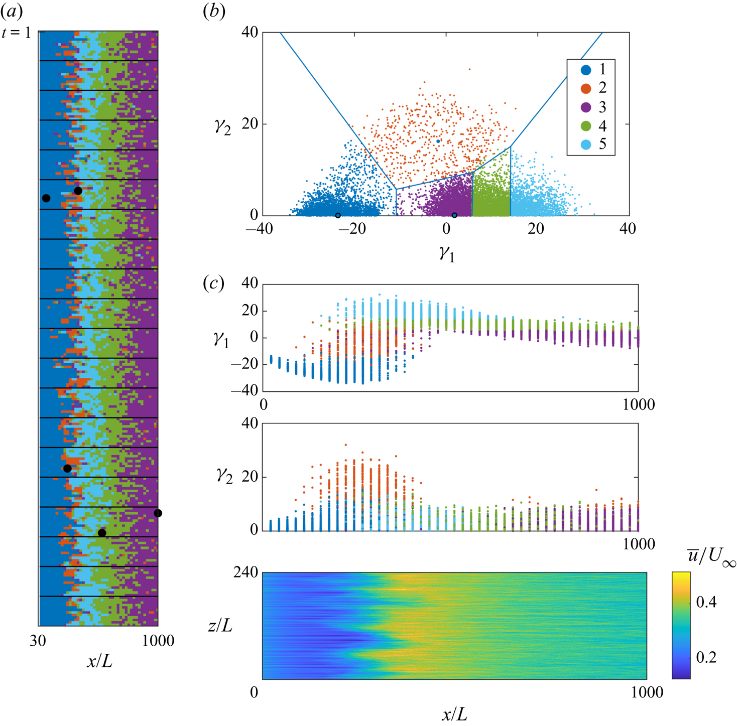
Clusters 2 and 3 in figure 9(a) are now merged into the cluster 2 and subsequent clusters are renamed. Figure 10(a) shows the contour representation of the clustered super-domain reconstruction for five clusters in different colours, containing all the 20 time steps. The super-domain contains the full spatial domain ( $x$–
$x$– $z$ plane) in every time step located below each other. Thus, the horizontal axis is the streamwise location steps of the cells, and the vertical axis consists of spanwise location steps repeated in time steps. Continuous black lines separate different time observations.
The scatter plots of  $\gamma _1$ and $\gamma _2$ in the streamwise direction are shown in figure 10(a). In order to obtain a better analysis of these plots, the time-averaged flow domain is also shown in the lowest section. In this domain, the evolution of the turbulent boundary layer along the streamwise direction can be seen. The region of transition in both plots of $\gamma _1$ and $\gamma _2$ is clearly visible, where these parameters have large variance. The points on these plots are coloured by different clusters, which shows their distribution along the flow direction. This analysis gives us a clear idea about different regions in the flow, especially the transition region, without any further knowledge of the physics of the flow.
The corresponding medoids for the five clusters are visualized in figure 11, in which we can detect different structures inside different medoids. Implementing the  $K$-medoids algorithm, we know that each medoid corresponds to one of the observations. So, these medoids are representative of their corresponding clusters, and thus, the difference between their internal structure reveals the different flow regimes. Cluster 1 represents the laminar region containing the streaks; cluster 2 contains the turbulent spots which are located in the transition stage; cluster 3 is the fully turbulent stage; cluster 4 and 5 show two intermediate regions of turbulence amplifications starting in the transition region.
Original contour illustration of the cluster medoids; showing the streaks in (a) medoid 1, (b) turbulent spots in medoid 2 and (c–e) turbulent stages in medoids 3 to 5 with increasing in intensity.
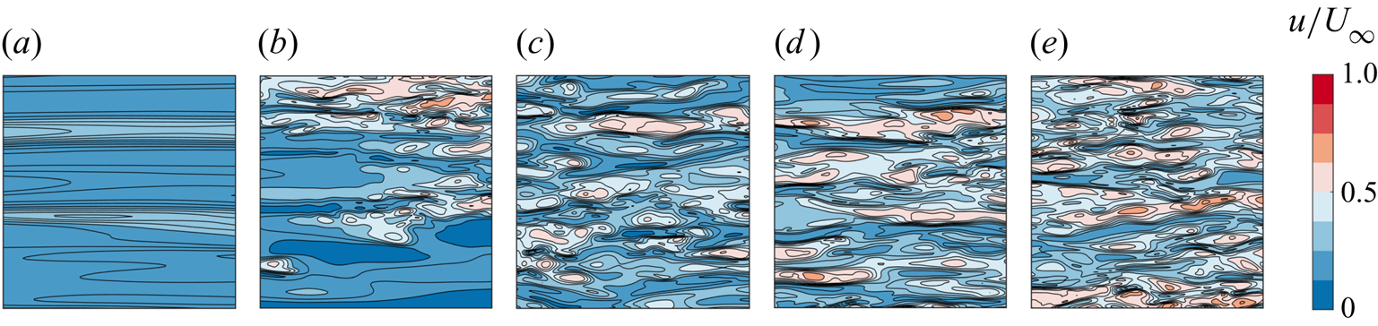
4. Dynamical analysis
In section § 3, the analysis was done to coarse-grain the cells into clusters. In this section, a dynamical model with no user input for the cluster transitions is elaborated in the form of a Markov chain. The temporal dynamics is extracted via a probabilistic network of transitions derived from the data. A simplified approach is implemented, defined here as pseudo-Lagrangian. The approach exploits the construction of the domain, in which the time separation between snapshots is equal to one convection time along the cell. Consequently, moving forward of one cell in the streamwise position and one step forward in time is equivalent to track the cell evolution. This is an approximation, which greatly simplifies the analysis, although is subject to assuming a uniform and constant convection velocity along the domain. A fully Lagrangian approach would require tracking individual fluid parcels over time to track the evolution. While this simplification will have an impact on the quantitative information of the probabilistic model of the dynamics, it is not expected to have a significant impact on the extracted qualitative information.
The analysis starts with the determination of the CTM, following the cluster-based reduced-order modelling (known as CROM) methodology (Kaiser et al. Reference Kaiser2014a). The tool is the transition probability matrix (see § 2.4), which is necessary to make state forecasts. This matrix provides the probability of a cell transitioning from one cluster to another within a given forward time step  $\Delta t$. The time step is constant and small as compared with the characteristic time scale of the flow. This matrix represents a discrete time step mapping. In the following sections, the temporal evolution of a general cluster probability vector is pursued. The distance matrix and the CTM are provided and analysed. Finally, the pseudo-Lagrangian tracking technique provides the dominant trajectories in the cluster space.
The transition probability of every cluster represents the dynamical change of state in the entire flow field. In other words, by analysing the transitions between clusters, the transition dynamics between characteristic phases of the flow can be deduced.
The tool that helps us discover the similarity of the clusters that have the most transition probability in common is the cluster distance matrix, which contains the values of distances between each two medoids in 2-D space. The distance parameter in the low-dimensional space of observations reconstructs the dissimilarity of the primitive cells. This matrix allows us to analyse the geometric relation of the medoids. Having the cluster distribution geometry along with their temporal transition probabilities generates a dynamical model of the cluster evolution and, accordingly, of the regions of the flow field. These two matrices are shown in figure 12. In this figure, the scale for the distance matrix is linear, while it is logarithmic for the transition matrix. In figure 12(a) the colours indicate the transition probability  $P_{jk}$, while in figure 12(b) they indicate the distance between clusters, and that the same information is also reported in the form of circles to enhance the interpretability. High values of the probabilities in the principal diagonal refer to intracluster persisting.
Accordance of kinematic and dynamical analysis: (a) CTM; (b) cluster distance matrix. The values are depicted by filling colours and with the radius of the corresponding circle. For the transition matrix the scale is logarithmic, while it is linear for the distance matrix. Cluster subsets are shown in black squares.
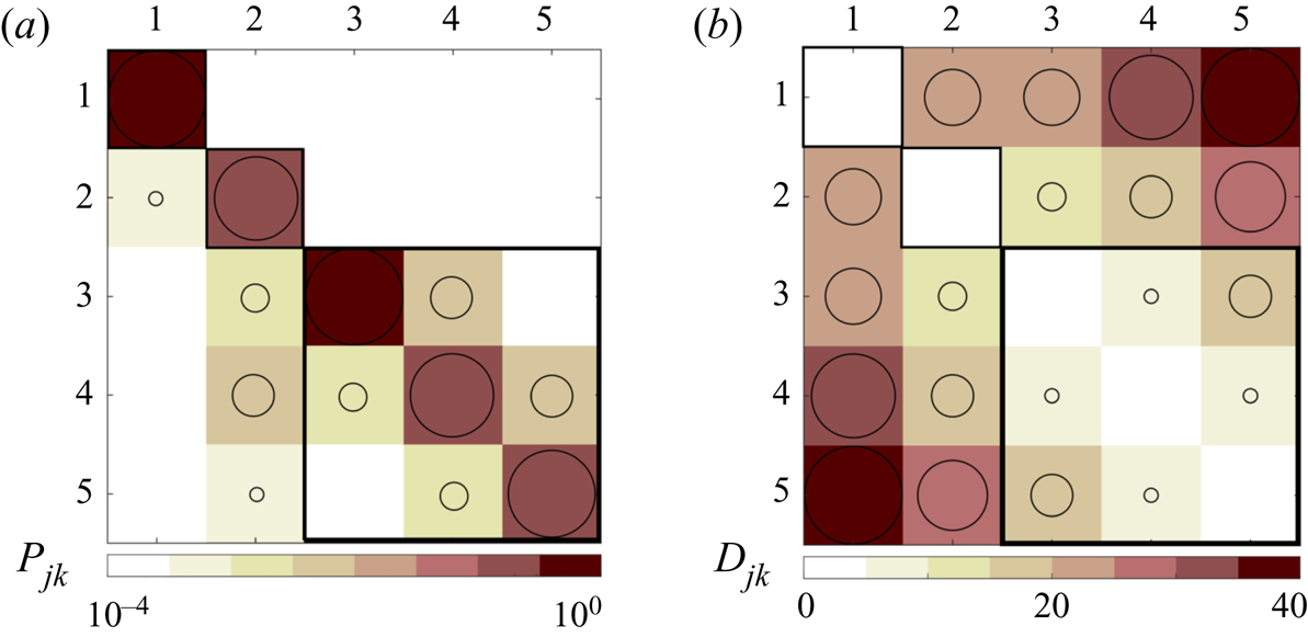
The transition matrix reveals three subsets of clusters that are enclosed in black squares. Clusters 1 and 2 are separated as individuals, while clusters 3, 4 and 5 are gathered within one subset, meaning that the transition between them is more likely. The criterion for the separation of the subsets in the CTM is to maximize the probability inside the subsets and minimize the probability outside subsets, and the opposite for the distance matrix. It can be done by applying any clustering strategy on these values. Those three clusters that form one subset are closer to each other with respect to the other clusters, and the transition probabilities between them are the largest. While the probability of going from this subset to other clusters is almost negligible, they represent a final state, and indeed are representative of the fully turbulent state of the flow.
The cluster groups are visible in the distance matrix as well, and it means that the cluster medoids are closer to each other in the 2-D space, i.e. are representative of similar flow behaviours. It also shows the accordance of the kinematic and dynamical analysis of this work. Here the common denominator for grouped clusters is that a fully turbulent state has been achieved. Following the higher probability paths, the matrix shows that cells in cluster  $C_1$, which is the region containing the streaks, will mostly remain in the same state after one time step as the probability $P_{11}$ is high. With lower probability, they can move to the second cluster, in which the dominant physical behaviour is the turbulent spots. Then from this cluster, cells can stay there or move forward in the direction towards clusters 3, 4 or 5. In cluster $C_3$, the probability of remaining in the same state is large and, thus, it reveals the state of fully turbulent. We should note that for returning to the initial states, there is almost no possibility. Cluster $C_2$ has a special significance as a ‘transient cluster’, acting as a switch between two main regions of streaks and turbulence. As elaborated above, this cluster resembles an intermediate state and links both regimes.
To track the transition of cluster states in continuous time steps, we need to extract the pseudo-Lagrangian trajectory of cells from the leading edge to the end of the plate, as stated in section § 2.4. An accumulation graph of trajectories from the beginning to the end of the domain is shown in figure 13(a). The dynamics can be observed from the trajectories in this clustered 2-D space. Since different points of a cluster have different trajectories, the most probable trajectories are determined. Again, following the trajectory graph reveals the cluster evolution was starting from cluster 1 (streaks), and terminating in cluster 3. It can be seen in figure 13(b) that the typical path is consistent with the CTM, and the cells typically move from streaks to turbulent spots (not necessarily centred in the domain), to regions with high streamwise variance (turbulence amplification) and finally to regions in the centre which is the most spatially homogeneous configuration, thus fully developed turbulence.
Dynamical analysis: (a) cluster transition trajectories are plotted between the cluster medoids on the clustered 2-D map of the data points, coloured by the cluster naming; (b) graph of the most probable cluster transition trajectory. The group of the three final clusters are depicted in one specific colour to show their belonging to the turbulent region.
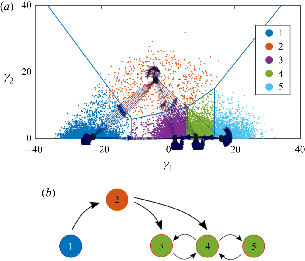
5. Conclusions
In the present work, cluster analysis and a dimensionality reduction approach, as unsupervised ML techniques, are applied to a DNS dataset of an incompressible boundary layer flow developing over a flat plate in an attempt to verify whether unsupervised tools can automatically identify the steps of boundary layer transition. A wall-parallel plane at a relatively small distance from the wall has been selected, as intuitively it is the region where most of the transition-related flow features are expected to be spotted. Wall-parallel planes have been subdivided into small regions corresponding to local observations. The observation matrix forms a high-dimensional dataset that has been reduced to a 2-D dataset using MDS. Taking advantage of MDS, we can significantly reduce the dimensionality of the problem, while preserving the data structure in the state space. Multidimensional scaling is able to provide a significant insight since the two dimensions are representative of the streamwise turbulence intensity and of the skewness of the turbulence intensity distribution in the spanwise direction. While the problem is expected to be one-dimensional, the presence of a second coordinate is a direct consequence of not choosing an aspect ratio for the cells. Here such a choice would be trivial, but in the most general scenario this might not be the case and setting an aspect ratio beforehand would have induced a bias of the observer. The focus of the present work is on how much human intuition can be replicated in an ‘automatic’ manner. For this reason, choosing an aspect ratio of the cells equal to unity leads to two relevant directions in the MDS, the second one being actually a spurious product of the translational invariance.
Following the MDS, the  $K$-medoids clustering algorithm is used to partition the domain, such that the medoids of each cluster represent the local flow states. With this feature-space discretization, we obtained a domain partitioning which consists of five different regions. As a result, the regions of development of a transitional boundary layer are automatically identified as regions containing streaks, turbulent spots, amplification of disturbances and fully developed turbulent flow.
In this work, the pseudo-Lagrangian evolution of the regions and the state transitions are employed in terms of a transition probability matrix and transition trajectory graph to determine flow dynamics and transition mechanisms between the different states. The development of regions in transitional boundary layer flow presents intermediate stages that create two alternative paths for transition development. The present methodology correctly identifies the bypass transition mechanism. This work thus shows that unsupervised algorithms can identify complex flow dynamics and provide simple models of the dynamics of transitional and streamwise-evolving flows. Such an approach, which has shown to be rather free from human input, could be used in the future to shed light on complex streamwise evolving flows, including those non-homogeneous in the spanwise direction, such as the developing boundary layers over a rotating blade, a swept wing or in a bent pipe.
Funding
This work has been supported by: (i) the Madrid Government (Comunidad de Madrid) under the Multiannual Agreement with UC3M in the line of ‘Fostering Young Doctors Research’ (PITUFLOW-CM-UC3M), and in the context of the V PRICIT (Regional Programme of Research and Technological Innovation); (ii) the COTURB project (Coherent Structures in Wall-bounded Turbulence), funded by the European Research Council (ERC), under grant ERC-2014.AdG-669505.
Declaration of interests
The authors report no conflict of interest.


 Open access