


1. Introduction
Electromagnetic surface waves are electromagnetic waves that propagate along an interface (surface) between different media. Their defining feature is that they are localized near the interface because they are evanescent in both directions normal to the interface. They were initially studied in isotropic media, where Epstein (Reference Epstein1954) concluded they can only exist if the electric permittivity changes sign at the material interface. Since this is common wherever an unmagnetized plasma is in contact with a dielectric solid, surface waves have long been known to be relevant to plasma physics (see e.g. Kaw & McBride Reference Kaw and McBride1970; Aliev et al. Reference Aliev, Berndt, Schlüter and Shivarova1995, Reference Aliev, Aliev, Schlüter, Schlüter and Shivarova2000; Lee & Lee Reference Lee and Lee2010; Girka, Girka & Thumm Reference Girka, Girka and Thumm2016; Lee, Shahmansouri & Jung Reference Lee, Shahmansouri and Jung2019; Maquet & Messiaen Reference Maquet and Messiaen2020; Girka, Girka & Thumm Reference Girka, Girka and Thumm2020). If the plasma in question is the electron plasma in a solid conductor, the surface waves are ‘surface plasmons’ (Ritchie & Marusak Reference Ritchie and Marusak1966; Gangaraj & Monticone Reference Gangaraj and Monticone2019).
Physically, in the context of electromagnetic waves in magnetized plasmas in the ion cyclotron range of frequencies (ICRF), surface waves may cause parasitic heating (Messiaen & Maquet Reference Messiaen and Maquet2020), play a role in interactions between electromagnetic waves and filaments in the edge plasma (Lau et al. Reference Lau, Bertelli, Myra, Ram, Shiraiwa, Tierens, Brookman, Dimits, Dudson and Martin2020; Tierens, Zhang & Manz Reference Tierens, Zhang and Manz2020a; Tierens, Zhang & Myra Reference Tierens, Zhang and Myra2020b) or occur as ‘sheath–plasma waves’ (Myra et al. Reference Myra, D'Ippolito, Forslund and Brackbill1991; Myra & D'Ippolito Reference Myra and D'Ippolito2009) on the ‘interface’ formed by the sudden and steep plasma density decrease in the plasma sheath.
In numerical ICRF calculations, non-physical surface waves often arise when an artificial discontinuity is introduced in the plasma density profile. A common reason to introduce this density jump is the desire to avoid numerical issues associated with the numerical resolution of the lower hybrid resonance, such as those described by Nicolopoulos, Campos-Pinto & Després (Reference Nicolopoulos, Campos-Pinto and Després2019). In such calculations, much of edge plasma density gradient is replaced by a single density jump, on which numerical surface waves often occur. This is not without exception: Brambilla & Bilato (Reference Brambilla and Bilato2021) report that in TORIC, an ICRF code which includes the full toroidal tokamak geometry, surface waves and related phenomena such as waveguide modes are rarely observed.
More generally, numerical surface waves may occur whenever a wave problem with material parameters that rapidly change in one spatial direction is approximated by a wave problem in a ‘slab geometry’ where rapidly changing material parameters are replaced by piecewise-constant material parameters (Messiaen & Weynants Reference Messiaen and Weynants2011). We discuss how introducing such density jumps can have numerical side effects caused by the presence of surface waves at the interface. For example, fields at the interface may not converge, and perfectly matched layers (PMLs), a type of absorbing boundary layer, may locally generate rather than absorb power.
In this paper we derive dispersion relations for surface waves in slab geometry in isotropic and anisotropic media, i.e. we derive a functional relation between the wave frequency and the wavevector tangent to the interface, via the dielectric tensors at both sides of the interface. After a brief description of the kind of waves we look for in § 2, we give two equivalent mathematical procedures for deriving the surface wave dispersion relation in §§ 3 and 4. We also derive low-order corrections to these dispersion relations when the material interface is steep but not discontinuous in § 4.2. Examples and convenient approximate expressions for the dispersion relation of surface waves on an interface between vacuum and magnetized plasma are presented in § 5. Sections 6 and 7 contain a discussion of undesirable numerical side effects of surface waves. The conclusion is given in § 8.
2. Surface waves on an interface between two media
In this work, we look for solutions of the one-dimensional electromagnetic wave equation. In Cartesian coordinates, we consider a planar material interface in the $x=0$ plane, so $x$
 is the normal direction and $y$
 and $z$
 the tangential directions. In the case of a magnetized plasma, we take the external magnetic field direction along $z$
 . We consider solutions with given tangential wavenumbers $k_y$
 and $k_z$
 in the $y$
 and $z$
 directions and $\exp (-\textrm {i}\omega t)$
 for the time dependence. The electric field $\boldsymbol {e}(x)\exp (\textrm {i} k_y y + \textrm {i} k_z z)$
 obeys the wave equation

where $\boldsymbol {\epsilon }(x)$ may be either scalar or a $3\times 3$
 matrix. We initially consider the discontinuous case, with a ‘left’ material and a ‘right’ material:
Later, we also consider steep continuous material parameter changes. Note that in the absence of surface currents the boundary conditions of Maxwell's equations demand that $e_y$ , $e_z$
 , $(\boldsymbol {\nabla }\times \boldsymbol {e})_y$
 and $(\boldsymbol {\nabla }\times \boldsymbol {e})_z$
 are continuous at $x=0$
 .
.
In this context, we seek solutions of the wave equation that are ‘surface waves’, localized near the surface $x=0$ , evanescent in both directions:

We use a slightly stronger notion of evanescence: a wave is evanescent in the positive $x$ direction if it is locally integrable on $[0,\infty [$
 and $\int _0^{\infty } \boldsymbol {e}(x)\,{\textrm {d}x}$
 converges. A wave is evanescent in the negative $x$
 direction if it is locally integrable on $]-\infty ,0]$
 and $\int _{-\infty }^{0} \boldsymbol {e}(x)\,{\textrm {d}x}$
 converges. These notions of evanescence are global, not local, properties of $\boldsymbol {e}(x)$
 . According to (2.3), a surface wave exists in the absence of incident waves (otherwise, the boundary condition at $\pm \infty$
 would have a non-zero amplitude of an incident wave). Since they do not receive energy, they cannot radiate energy; in this simplified description the wave cannot become propagative (i.e. radiating) some distance away from the surface, and a global notion of evanescence is required to guarantee this.
3. Spectral surface impedance matrices
Let us consider the four degrees of freedom $e_y, e_z, (\boldsymbol {\nabla }\times \boldsymbol {e})_y, (\boldsymbol {\nabla }\times \boldsymbol {e})_z$ that must be continuous across $x=0$
 . Instead of $\boldsymbol {\nabla }\times \boldsymbol {e}$
 , we may use $\boldsymbol {b}\equiv ({1}/{\text {i}\omega }\boldsymbol {\nabla })\times \boldsymbol {e}$
 , and demand the continuity of $e_y, e_z, b_y, b_z$
 .
.
Brambilla (Reference Brambilla1995) defines a surface impedance matrix ${\boldsymbol{\mathsf{Z}}}$ such that
The matrix ${\boldsymbol{\mathsf{Z}}}$ is a convenient way to impose two conditions between the four possible waves in the left or right material. This could be used to eliminate two of the modes, but other constraints are possible. For the right material ($x>0$
 ), ${\boldsymbol{\mathsf{Z}}}$
 is fully defined once:
(i) The $x$
 -dependent variations of the dielectric tensor are prescribed.
(ii) Boundary conditions are enforced at some place $x>0$
.


Here, as in Brambilla (Reference Brambilla1995), we take (3.1) to encode the condition that the solution is causal, i.e. with incident waves only from $x=-\infty$ , and radiation boundary conditions at $x=+\infty$
 . Equation (3.1) holds for both left and right materials, with surface impedance matrices ${\boldsymbol{\mathsf{Z}}}_L$
 and ${\boldsymbol{\mathsf{Z}}}_R$
 , respectively. The reflection at the interface between the two materials is, according to (14) in Brambilla (Reference Brambilla1995),

Equation (3.2) uses the following result: in the left material, the matrix ${\boldsymbol{\mathsf{Z}}}_L$ with right-going waves only is the opposite of the matrix ${\boldsymbol{\mathsf{Z}}}_L$
 with left-going waves only (radiation boundary conditions at minus infinity). For homogeneous cold magnetized plasmas, this relation only holds if the confining magnetic field is parallel to the interface.
Surface waves exist only if (3.2) has non-trivial solutions in the absence of incident waves, i.e. when $\text {det}({\boldsymbol{\mathsf{Z}}}_L+{\boldsymbol{\mathsf{Z}}}_R)=0$ . Throughout this work, we use vertical lines for the determinant, so $|{\boldsymbol{\mathsf{Z}}}_L+{\boldsymbol{\mathsf{Z}}}_R|=0$
 .
.
The polarization of the surface wave at $x=0$ is the nullspace (kernel) of ${\boldsymbol{\mathsf{Z}}}_L+{\boldsymbol{\mathsf{Z}}}_R$
 :
:

3.1. Example: surface waves on a discontinuous interface between isotropic media
For an isotropic dielectric with relative dielectric constant $\epsilon$ and radiative boundary conditions at $x\rightarrow +\infty$
 , the surface impedance matrix is

where $\boldsymbol {n}=c \boldsymbol {k}/\omega$ . Here $n_x$
 is real for propagating waves and purely imaginary for evanescent waves. The existence condition for surface waves, $|{\boldsymbol{\mathsf{Z}}}_L+{\boldsymbol{\mathsf{Z}}}_R|=0$
 , becomes

with $n_{x,L}=-\textrm {i}\sqrt {n_y^{2}+n_z^{2}-\epsilon _L}$ and $n_{x,R}=\textrm {i}\sqrt {n_y^{2}+n_z^{2}-\epsilon _R}$
 . This yields the surface wave dispersion relation:

Solving for $n_y^{2}+n_z^{2}$ gives
gives

4. Laplace representation
Another way to derive the dispersion relation for surface waves is based on the Laplace transform of the wave equation in the right domain (assuming, for now, that $\boldsymbol {\epsilon }_R$ is spatially constant). Using $\boldsymbol {E}(s)$
 for the Laplace-transformed electric field components and $\boldsymbol {e}(x)$
 for the untransformed electric field components:

where we assume $\boldsymbol {e}(x)$ is locally integrable on $[0,\infty [$
 , and we use the strong notion of evanescence from § 2: $\boldsymbol {e}(x)$
 is evanescent if $\int _0^{\infty } \boldsymbol {e}(x)\,{\textrm {d}x}$
 converges, that is, if (4.1) converges for all $\textrm {Re}(s)\geq 0$
 , that is, if $\boldsymbol {E}(s)$
 has no poles with $\textrm {Re}(s)\geq 0$
 .
.
The Laplace transform of the wave equation (2.1) is

where $\boldsymbol {e}'(x)$ is the first derivative ${\partial \boldsymbol {e}}/{\partial x}$
 . The condition of no contributions from non-evanescent waves is that the Laplace-transformed electric fields must have no poles in the right half-plane (i.e. with positive real part). From (4.2) we easily see that poles can only exist where

with

which is precisely the dispersion relation of the waves in the $\boldsymbol {\epsilon }_R$ material, up to substitution $s\rightarrow i k_x$
 . For brevity, let us also define

The reasoning that follows is generally valid for both isotropic and anisotropic media, but certain details are different, which are discussed in § 4.3. For the moment, in addition to the assumption that $\boldsymbol {\epsilon }_R$ is spatially constant, let us also assume that the material is isotropic, so (4.3) has two distinct double roots (as opposed to four distinct single roots in the anisotropic case), one root with $\textrm {Re}(s)<0$
 and one with $\textrm {Re}(s)>0$
 . Let $s=s_0$
 be the root with $\textrm {Re}(s)>0$
 . At $s=s_0$
 , the matrix ${\boldsymbol{\mathsf{M}}}_{0}(\boldsymbol {\epsilon }_R,s_0)$
 has rank 1, the dimension of the column space is 1, all columns are linearly dependent. Thus, there is a non-zero $2\times 3$
 matrix ${\boldsymbol{\mathsf{N}}}_{s_0}$
 of rank two such that

Equivalently, the rows of ${\boldsymbol{\mathsf{N}}}_{s_0}$ span the nullspace of ${\boldsymbol{\mathsf{M}}}_{0}(\boldsymbol {\epsilon }_R,s_0)^\textrm {T}$
 .
.
Left-multiplying (4.2) at $s=s_0$ by ${\boldsymbol{\mathsf{N}}}_{s_0}$
 then yields

The condition (4.7) is a necessary condition for there to be no contribution from the non-evanescent mode.
Note that $e_x(0)$ is not an independent degree of freedom: the $x$
 component of the one-dimensional wave equation (2.1) is an algebraic equation, not a differential equation, in $e_x$
 , and can be solved directly:

Equation (4.8) is valid in general, for any dielectric tensor including anisotropic ones, whose components we write as $\boldsymbol {\epsilon }_{R,ij}$ . Thus, we can construct a $5\times 4$
 matrix ${\boldsymbol{\mathsf{T}}}(\boldsymbol {\epsilon }_R)$
 such that

Then, (4.7) becomes

This $2\times 4$ matrix enforces that there is no contribution of non-evanescent modes in the right material. We analogously construct such a $2\times 4$
 matrix in the left material, yielding a total of four linear homogeneous constraints in four unknowns. Setting the determinant to zero then gives the surface wave dispersion relation.
4.1. Example: surface waves on a discontinuous interface between isotropic media
In this subsection we re-derive the result of § 3.1, this time using the Laplace formalism, in order to illustrate the equivalence of these approaches. For scalar $\epsilon _R$ , (4.3) gives us possible poles at $s_0=\pm \sqrt {k_y^{2}+k_z^{2}-({\omega ^{2}}/{c^{2}})\epsilon _R}$
 . The one with positive real part is $s_0=\sqrt {k_y^{2}+k_z^{2}-({\omega ^{2}}/{c^{2}})\epsilon _R}$
 . Then

which gives us ${\boldsymbol{\mathsf{N}}}_{s_0}$ according to (4.6). The matrix ${\boldsymbol{\mathsf{T}}}(\epsilon _R)$
 obeying (4.9) is given by (4.36). Finally, the two rows encoding the condition that there are no poles with positive real part/no non-evanescent contributions in the right material are

For the left material we follow the same line of reasoning once again. Instead of using a non-standard ‘Laplace transform’ along the negative real axis, it is more convenient to mirror the left material, so that the mirrored left material exists at $x>0$ just like the right material. Then, we can follow the reasoning of § 4 without modifications. When we get the $2\times 4$
 matrix analogous to (4.12), we merely need to ‘mirror’ it back, an operation under which the tangential magnetic field, being a pseudovector, changes sign, accordingly

Putting the rows from the left and right material together yields the surface wave dispersion relation:

which becomes

To see that (4.15) is equivalent to (3.7), first note $s_{0,R}=-\textrm {i} k_{x,R}$ and $s_{0,L}=\textrm {i} k_{x,L}$
 ($s_{0,L}$
 and $s_{0,R}$
 both have positive real part; $k_{x,L}$
 ($k_{x,R}$
 ) are wavenumbers for waves evanescent towards negative (positive) $x$
 , hence the different sign). With $k_{x,L}=-\textrm {i}\sqrt {k_y^{2}+k_z^{2}-{\epsilon _L\omega ^{2}}/{c^{2}}}$
 and $k_{x,R}=\textrm {i}\sqrt {k_y^{2}+k_z^{2}-{\epsilon _R\omega ^{2}}/{c^{2}}}$
 , then

which is indeed (3.7). Continuing,


Recall that the denominator $k_y^{2}+k_z^{2}-{\epsilon _R \omega ^{2} }/{c^{2}}$ is positive, so (4.18) tells us that ${\epsilon _L}/{\epsilon _R}$
 must be negative, i.e. that $\epsilon _L$
 and $\epsilon _R$
 must have opposite sign. This is a classical result in the study of electromagnetic surface waves in isotropic media, going back to Epstein (Reference Epstein1954).
4.2. Generalization to steep continuous material interfaces
Let us now consider $\boldsymbol {\epsilon }_R=\boldsymbol {\epsilon }_{R,1}+\boldsymbol {\epsilon }_{R,2}\exp (-\alpha x)$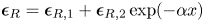 , with $\alpha >0$
 , and ${\boldsymbol {\epsilon }_{2,11}}/{\boldsymbol {\epsilon }_{1,11}}> -1$
 , such that $\boldsymbol {\epsilon }_{11}(x)=\boldsymbol {\epsilon }_{1,11}+\boldsymbol {\epsilon }_{2,11}\exp (-\alpha x)$
 has no roots with $x\geq 0$
 . The steepness parameter $\alpha$
 has units of m$^{-1}$
 . Large $\alpha$
 correspond to a steep gradient, and we expect to retrieve the discontinuous case in the $\alpha \rightarrow \infty$
 limit. In plasma, this will allow us to consider surface waves on smooth density gradients such as (5.18), provided they do not cross the lower hybrid resonance.
The Laplace-transformed wave equation now becomes

Again, we wish to ensure that the Laplace representations of the fields in the right domain have no poles with positive real part, which would correspond to contributions of non-evanescent modes. We can always consider the pole with largest real part first, so we consider the possibility that some component of $\boldsymbol {E}(s)$ diverges at some $s=s_0$
 , but $\boldsymbol {E}(s_0+\alpha )$
 remains finite. Clearly this can only occur where

which is the asymptotic (large $x$ ) dispersion relation, up to substitution $s\rightarrow \textrm {i} k_x$
 . Again assuming an isotropic medium (for the anisotropic case, see § 4.3), (4.20) has two double roots, and we pick the root $s=s_0$
 with positive real part. We can again find a non-zero $2\times 3$
 matrix ${\boldsymbol{\mathsf{N}}}_{s_0}$
 of rank 2 such that

Left-multiplying (4.19) at $s=s_0$ by ${\boldsymbol{\mathsf{N}}}_{s_0}$
 then yields

At this point, we must assume $\alpha$ is large (the interface is steep), so we can insert asymptotic expressions for $\boldsymbol {E}(s_0+\alpha )$
 . In Appendix A we show


where the condition ${\boldsymbol {\epsilon }_{2,11}}/{\boldsymbol {\epsilon }_{1,11}}\geq -1$ is necessary for the convergence of (4.23), and

For brevity, let us write

then

For further brevity, define

then

Finally, inserting (4.30), (4.24) and (4.25) in (4.22) gives

Comparing (4.31) with (4.7), we see that a correction term, accounting for finite interface steepness, has appeared. Recalling (4.9) we finally get

Equation (4.32) is a $2\times 4$ matrix, representing two rows of the $4\times 4$
 matrix whose determinant must be zero for surface waves to exist. The other two rows are obtained by constructing the equivalent of (4.32) in the left domain.
For finite-steepness effects to be negligible, the correction term in (4.31) has to be negligible with respect to the first term. Let $\| \cdot \|$ denote a matrix norm:

Let us briefly discuss the condition ${\boldsymbol {\epsilon }_{2,11}}/{\boldsymbol {\epsilon }_{1,11}}> -1$ , which we imposed in this section. Condition ${\boldsymbol {\epsilon }_{2,11}}/{\boldsymbol {\epsilon }_{1,11}}\geq -1$
 is necessary for (4.23) to exist. Condition $\boldsymbol {\epsilon }_{11}(0)\neq 0$
 , that is, ${\boldsymbol {\epsilon }_{2,11}}/{\boldsymbol {\epsilon }_{1,11}}\neq -1$
 , is necessary for ${\boldsymbol{\mathsf{T}}}$
 to exist. Thus, we can use the reasoning of this section only for material interfaces where $\boldsymbol {\epsilon }_{11}$
 does not change sign, and we cannot use it for density gradients that cross the lower hybrid resonance.
4.3. Anisotropic case
The Laplace-domain constructions of the previous subsections do not crucially depend on having an isotropic medium. In the isotropic case, the dispersion relation (4.3), respectively (4.20), had one double root with positive real part. The Laplace-transformed wave equation at this point could be left-multiplied by a $2\times 3$ matrix ${\boldsymbol{\mathsf{N}}}_{s_0}$
 obeying (4.6), respectively (4.21), reducing it to two scalar equations, two rows of the $4\times 4$
 matrix whose determinant must be zero for surface waves to exist.
In the anisotropic case, there are two distinct single roots of the dispersion relation with positive real part. At each one, the Laplace-transformed wave equation can be left-multiplied by a non-zero $1\times 3$ matrix ${\boldsymbol{\mathsf{N}}}_{s_0}$
 obeying (4.6), respectively (4.21), reducing it to one scalar equation for each root, so two in total, still two rows of the $4\times 4$
 matrix whose determinant must be zero for surface waves to exist.
4.4. Explicit expressions for ${\boldsymbol{\mathsf{N}}}_{s_0}$ and ${\boldsymbol{\mathsf{T}}}$


Define

such that

Then

Vacuum is isotropic, so ${\boldsymbol{\mathsf{N}}}_{s_0}$ is a $2\times 3$
 matrix. The wave modes are evanescent if $k_y^{2}+k_z^{2}-{\omega ^{2}}/{c^{2}}>0$
 . Then


Stix (Reference Stix1992) gives the dielectric tensor in cold magnetized plasma:

With this dielectric tensor, the equation defining $s_0$ , (4.20), is biquadratic. In anisotropic magnetized plasma, we have two $1\times 3$
 matrices ${\boldsymbol{\mathsf{N}}}_{s_0}$
 , one for each of the two $s_0$
 roots with positive real part, provided two evanescent wave modes do indeed exist:


5. Examples
5.1. Surface waves on a vacuum–plasma interface in the ICRF regime
5.1.1. Approximate dispersion relation for fast wave surface waves on a plasma–vacuum interface, in the limit of infinite parallel conductivity
The surface impedance matrix for an infinite vacuum layer at $x<0$ is, according to (13) in Brambilla (Reference Brambilla1995),

Brambilla & Bilato (Reference Brambilla and Bilato2021) also give the surface impedance matrix for a vacuum layer of finite thickness $d$ which ends on a perfectly conducting wall:

The cold plasma dielectric tensor is again (4.40). We consider the infinite parallel conductivity limit $\boldsymbol {\epsilon }_{\parallel } \rightarrow \infty$ . According to Messiaen & Weynants (Reference Messiaen and Weynants2011), the surface impedance matrix for cold plasma is, in that limit,

where


The subscript $F$ is for the fast wave, the only wave mode that exists in this limit. The surface wave dispersion relation becomes


This defines the dispersion relation of surface waves as a functional relation between $n_y$ and $n_z$
 . For an infinite vacuum layer ($d\rightarrow \infty$
 ), explicit approximate formulas for $n_y$
 as a function of $n_z$
 can be obtained in the asymptotic limit of large poloidal wavenumbers (high $n_y$
 ). In this approximation, a Taylor expansion in the small parameter $\sqrt {1-n_z^{2}}$
 , respectively $n_{\perp ,F}$
 , gives


which leads to the approximate surface wave dispersion relation:

Only positive values of $n_y^{2}$ are physically relevant. Infinite $n_y$
 , i.e. vertical asymptotes to the dispersion relation, are obtained for parallel refractive indices such that the denominator of the fractions vanishes. As $\omega |n_y|$
 becomes of the order of the electron plasma frequency $\omega _e=\sqrt {{n q^{2}}/{m_e\epsilon _0}}$
 , where $n$
 is the density, $q$
 the electron charge and $m_e$
 the electron mass, the approximation of infinite $\boldsymbol {\epsilon }_{\parallel }$
 becomes questionable and the fast wave might couple with the slow mode.
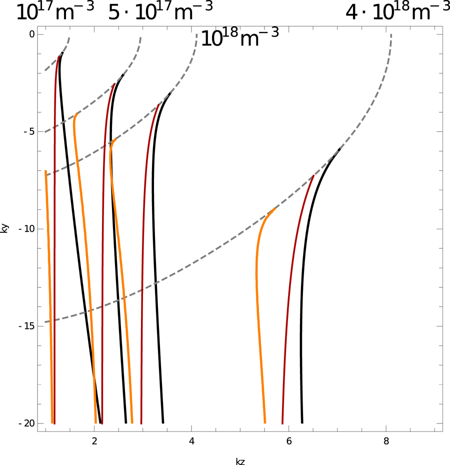
An example of this surface wave dispersion relation is shown in figure 1, under conditions typical in ASDEX Upgrade, with core hydrogen minority heating in deuterium plasma, a confining magnetic field strength of $B_0\approx 2$ T in the edge plasma near the antenna and an ICRF antenna frequency of $f=36.5$
 MHz. The dispersion relation is not symmetric in $k_y$
 : there is a preferred vertical propagation direction for such surface waves, in this case downward (negative $k_y$
 ). This is a common feature of surface waves (Gangaraj & Monticone Reference Gangaraj and Monticone2019), and is consistent with what we sometimes see in finite element simulations, such as in figure 2. We also show the case of finite vacuum layer thickness $d$
 . At short poloidal wavelengths, which is not unrealistic especially when considering spurious/numerical excitation of surface modes, where the poloidal spectrum of the surface waves often differs appreciably from that of the bulk waves, $d$
 can be larger than the decay length of the wave in vacuum, and the description of such waves as surface waves is appropriate. When the decay length of the wave in vacuum is comparable to $d$
 or larger, the wave mode is better described as a waveguide mode, a point also made in Brambilla & Bilato (Reference Brambilla and Bilato2021).
Dispersion relations of a surface wave on a discontinuous interface between vacuum and magnetized plasma, for various plasma densities, assumed spatially constant. Grey dashed: above this curve, the fast wave propagates. Solid red: approximate dispersion relation from § 5.1.1 in the $\boldsymbol {\epsilon }_{\parallel }\rightarrow \infty$ limit, with an infinite vacuum layer. Solid orange: the same, with a finite vacuum layer thickness of $d=5$
 cm. Solid black: full dispersion relation with finite $\boldsymbol {\epsilon }_{\parallel }$
 , with an infinite vacuum layer. Parameters are $B_0=2$
 T in the $z$
 direction, $f=36.5$
 MHz, deuterium plasma.
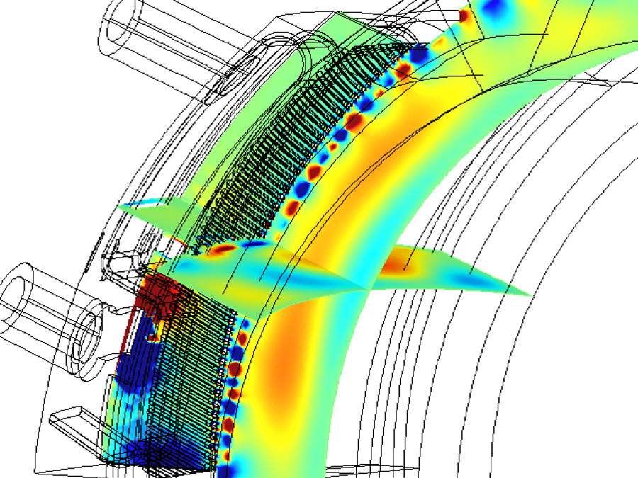
Surface waves are sometimes seen on the plasma–vacuum interface in the finite element RAPLICASOL code, an ICRF modelling code described in, for example, Tierens et al. (Reference Tierens, Milanesio, Urbanczyk, Helou, Bobkov, Noterdaeme, Colas and Maggiora2019) and López et al. (Reference López, Ochoukov, Tierens, Willensdorfer, Zohm, Aguiam, Birkenmeier, Bobkov, Cavedon and Dunne2019). It cannot be seen on this single image, but the surface waves are indeed moving downward, consistent with the negative $k_y$ seen in figure 1. The poloidal component of the Poynting vector is, on average, upward along the plasma–vacuum interface, indicating a mainly backward wave.
The negative $n_y$ branch of the approximate surface wave dispersion relation (5.12) attains a minimum possible $n_y ^{2}+n_z^{2}$
 at the point where $n_{x,F}^{2}=0$
 :
:

Correspondingly, it has a maximum possible vacuum evanescence length

In this approximation, the surface waves exist only for a finite range of parallel wavenumbers $k_z$ , which suggests ways to avoid exciting them. Physically, tailoring the $k_z$
 spectrum such as to avoid low $k_z$
 , consistent with Messiaen & Maquet (Reference Messiaen and Maquet2020) and Maquet & Messiaen (Reference Maquet and Messiaen2020), can prevent surface wave excitation at least in this $\boldsymbol {\epsilon }_{\parallel }\rightarrow \infty$
 approximation. Numerically, there is some design freedom in where to put the plasma–vacuum interface: it must be beyond the lower hybrid resonance, but before the point where the fast wave launched by the antenna becomes propagative (which depends on $k_y$
 ; the fast wave launched by the antenna typically has much larger poloidal wavelength than the surface waves), such that the fast wave evanescence layer, a crucial ingredient in ICRF power coupling calculations, is modelled as correctly as possible. Given a $k_z$
 spectrum that avoids low $k_z$
 , choosing the density jump small enough could reduce surface wave excitation.
5.1.2. The full surface wave dispersion relation on a plasma–vacuum interface
Using § 4, we can construct the full dispersion relation for surface waves on a plasma–vacuum interface. The simplifying assumption $\boldsymbol {\epsilon }_{\parallel }\rightarrow \infty$ is not necessary. Effectively, we use (4.38), (4.39), (4.41) and (4.42) to construct three copies of (4.10), one in vacuum (a $2\times 4$
 matrix) and two in plasma (two $1\times 4$
 matrices). Putting them together gives us a $4\times 4$
 matrix, let us call it ${\boldsymbol{\mathsf{L}}}(k_y,k_z,\omega )$
 , the zeros of the determinant of which give us the surface wave dispersion relation:

The resulting expressions are cumbersome, and we resort to evaluating them numerically. An example of this surface wave dispersion relation is shown in figure 1, compared with the approximate dispersion relations from § 5.1.1.
The surface wave phase velocity is

with $\omega (k_y,k_z)$ defined by the dispersion relation, and the group velocity is

A wave is usually called ‘forward’ if $\boldsymbol {v_{ph}\cdot v_g}>0$ and ‘backward’ if $\boldsymbol {v_{ph}\cdot v_g}<0$
 . Bécache, Joly & Kachanovska (Reference Bécache, Joly and Kachanovska2017) generalize this notion: a wave is forward, respectively backward, in the direction $\boldsymbol {d}$
 based on the sign of $(\boldsymbol {v_{ph}\cdot d})(\boldsymbol {v_{g}\cdot d})$
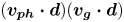 . Equivalently (see Appendix B), a wave is backward in either the $y$
 or $z$
 direction when ${\partial k_y^{2}}/{\partial k_z^{2}}>0$
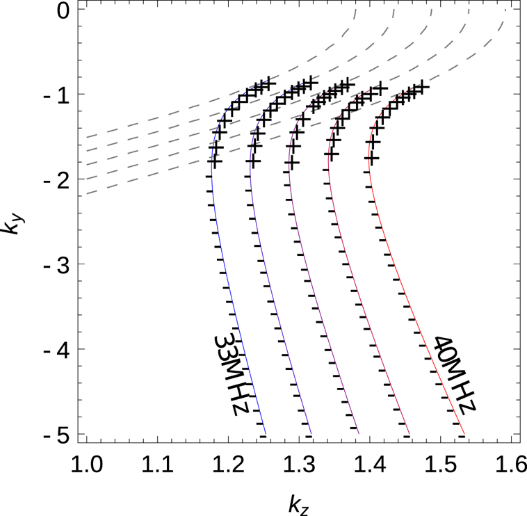
 . In figure 3 we see that the poloidal ($y$
 ) component of the group velocity changes sign depending on $k_y$
 , but the poloidal component of the phase velocity is negative. Thus, these surface waves can be either forward or backward in the poloidal direction, depending on $k_y$
 . Kousaka & Ono (Reference Kousaka and Ono2003) also report the numerical observation of both backward and forward surface waves. The approximate dispersion relation (5.12), valid in the $\boldsymbol {\epsilon }_{\parallel }\rightarrow \infty$
 limit, is always forward in the poloidal direction. With finite vacuum layer thickness (orange curves in figure 1), even the $\boldsymbol {\epsilon }_{\parallel }\rightarrow \infty$
 limit exhibits this behaviour. This has implications regarding the performance of PMLs, artificial absorbing boundary layers often used to terminate the simulation domain in finite element ICRF codes, which is further discussed in § 6.
Full surface wave dispersion relation on a plasma–vacuum interface with $n=10^{17}$ m$^{-3}$
 . Other parameters are as in figure 1. The dispersion relation is shown at frequencies ranging from $f=33$
 MHz (blue) to $f=40$
 MHz (red). The black line is where the surface wave changes from ‘forward’ to ‘backward’ in the $y$
 direction (poloidal). Above it, $\omega =2{\rm \pi} f$
 decreases with increasing $k_y$
 (so $\partial _{k_y}\omega <0$
 ), while $k_y$
 is negative; thus, these surface waves are forward in the $y$
 direction. Below it, $\omega$
 increases with increasing $k_y$
 (so $\partial _{k_y}\omega >0$
 ), while $k_y$
 is negative; thus, these surface waves are backward in the $y$
 direction. As in figure 1, the fast wave propagates above the grey dashed curves.

In the full surface wave dispersion relation, surface waves exist at wider ranges of $k_z$ than in the approximation of § 5.1.1. Surface waves can still be suppressed by introducing losses near the plasma–vacuum interface. A more extreme option is to artificially increase $\boldsymbol {\epsilon }_{\parallel }$
 near the plasma–vacuum interface. This has undetermined effects on the wave fields near the interface, but it reduces the $k_z$
 range in which surface waves can exist, and, by making the surface waves more forward, may even avoid the PML issues.
5.1.3. Surface waves on a plasma–vacuum interface where $\boldsymbol {\epsilon }_{\perp }$ does not change sign

All surface wave dispersion relations shown in figure 1 involve a surface between vacuum ($\boldsymbol {\epsilon }=1$ ) and a plasma that is dense enough that $\boldsymbol {\epsilon }_{\perp }<0$
 , that is, $\boldsymbol {\epsilon }_{\perp }$
 changes sign at the interface. We may consider the case where the plasma is less dense, such that $\boldsymbol {\epsilon }_{\perp }>0$
 . The approximate dispersion relations from § 5.1.1 still predict surface waves in this case, with both positive and negative $k_y$
 . In figure 4, we find corresponding roots in the full dispersion relation of § 5.1.2, only for positive $k_y$
 .
.
Dispersion relations of a surface wave on a discontinuous interface between vacuum and magnetized plasma, analogous with figure 1 but now with plasma density low enough that $\boldsymbol {\epsilon }_{\perp }$ remains positive in the plasma. Parameters are the same as in figure 1 except $n=10^{16}$
 m$^{-3}$
 . Solid red: approximate dispersion relation from § 5.1.1 in the $\boldsymbol {\epsilon }_{\parallel }\rightarrow \infty$
 limit. Solid black: full dispersion relation with finite $\boldsymbol {\epsilon }_{\parallel }$
 . The vacuum wave is evanescent outside of the orange lines, the (approximate) fast wave in the plasma is evanescent outside of the green lines and the slow wave is evanescent outside of the grey lines. For low positive $k_y$
 , the approximate dispersion relation (red) approximates the full dispersion relation (black). For negative $k_y$
 , the approximate dispersion relation (red) has no corresponding root in the full solution. The full solution is not shown, although it likely does exist in the region between the purple lines, where $k_x^{2}$
 is complex for the plasma waves.

5.1.4. Applicability of the slab-geometry model for surface waves on plasma–vacuum interfaces
If any physical phenomenon is approximately described by the results shown in § 5.1, it is that of surface waves on the steep edge density gradient in tokamaks (Messiaen & Maquet Reference Messiaen and Maquet2020). The physics of these surface waves is inextricably linked with that of the lower hybrid resonance, which leaves open questions about the validity of cold plasma descriptions. In any case, the theory of this paper does not include the lower hybrid resonance: discontinuous descriptions skip it entirely (numerically, this is often precisely the point of introducing a discontinuity), and the finite-steepness correction diverges in the presence of this resonance. Additionally, the curvature and density gradients on the plasma side are not taken into account.
Numerically, on the other hand, these results provide a near-perfect description of spurious surface waves excited on non-physical discontinuous density jumps from vacuum to plasma, which is discussed further in §§ 6 and 7.
5.2. Surface waves on plasma–plasma interfaces
Surface waves on plasma–plasma interfaces, with different density on both sides of the interface but without sign changes in $\boldsymbol {\epsilon }_{\perp }$ , are of physical interest since they may occur on the steep density gradients at the edge of the density filaments that naturally occur in tokamak edge plasmas (see e.g. Garcia Reference Garcia2009; Birkenmeier et al. Reference Birkenmeier, Manz, Carralero, Laggner, Fuchert, Krieger, Maier, Reimold, Schmid and Dux2015; Häcker et al. Reference Häcker, Fuchert, Carralero and Manz2018; Killer et al. Reference Killer, Shanahan, Grulke, Endler, Hammond and Rudischhauser2020; Lau et al. Reference Lau, Bertelli, Myra, Ram, Shiraiwa, Tierens, Brookman, Dimits, Dudson and Martin2020; Tierens et al. Reference Tierens, Zhang and Manz2020a,Reference Tierens, Zhang and Myrab). Messiaen & Weynants (Reference Messiaen and Weynants2011) show that they are also of numerical interest, since they may occur in slab-geometry approximations.
The Laplace approach lets us determine the surface wave dispersion relation in this situation, too. In figure 5, a surface wave dispersion relation on a sudden density change from $10^{17}$ to $10^{18}$
 m$^{-3}$
 is shown. It is qualitatively similar to the surface waves on plasma–vacuum interfaces.
(a) Black: surface wave dispersion relation on a sudden density change from $10^{17}$ to $10^{18}$
 m$^{-3}$
 at $x=0$
 . Other parameters are the same as in figure 1. The fast wave is propagative inside the grey dashed curve. Other dashed lines: finite steepness corrections, with $\alpha =50$
 m$^{-1}$
 (blue), $\alpha =75$
 m$^{-1}$
 (purple) and $\alpha =200$
 m$^{-1}$
 (red). (b) Corresponding density profiles.

5.2.1. Surface waves on steep continuous density changes in plasma
Figure 5 furthermore shows dispersion relations for surface waves on steeply changing density profiles of the form

derived as in § 4.2. Naturally, for high steepness $\alpha$ , the dispersion relations reduce to that derived for the discontinuous case.
The dispersion relation with finite steepness has an additional root, already partially visible in the top right of figure 5, where it displays a variety of forward and backward behaviour, and fully shown in figure 6. This new root has rapidly decreasing poloidal wavelength with increasing interface steepness, which may provide a qualitative explanation for a phenomenon that is observed numerically when modelling wave–filament interactions: surface waves on the steep density gradient at the filament have a poloidal wavelength that decreases with increasing steepness. In figure 6, the new root is forward (${\partial k_y^{2}}/{\partial k_z^{2}}<0$ ).
).
Dispersion relation for surface waves on a plasma–plasma interface under NSTX-relevant high-harmonic fast-wave conditions, $n_L=5\times 10^{16}~\textrm {m}^{-3}$ , $n_R=15\times 10^{16}~\textrm {m}^{-3}$
 , local confining magnetic field $B_0=0.55$
 T, frequency $30$
 MHz. Due to the finite steepness correction, there is a new root whose $k_y$
 increases with increasing steepness, which may provide a qualitative explanation for numerical observations under similar conditions such as those reported in Tierens et al. (Reference Tierens, Zhang and Manz2020a), where surface waves on filaments have azimuthal wavelengths that decrease with increasing steepness, as shown in the right-hand panels for a filament with a radius of 1 cm.

5.2.2. Applicability of the slab-geometry model for surface waves on plasma–plasma interfaces
Surface waves of ICRF on plasma–plasma interfaces may occur on the steep density gradients on filaments (Lau et al. Reference Lau, Bertelli, Myra, Ram, Shiraiwa, Tierens, Brookman, Dimits, Dudson and Martin2020; Tierens et al. Reference Tierens, Zhang and Manz2020a,Reference Tierens, Zhang and Myrab). Here, there is no $\epsilon _{\perp }$ sign change, no role of the lower hybrid resonance and no reason to expect warm plasma effects to come into play. Still, our slab-geometry model ignores curvature, which is questionable on these filaments of centimetre-scale radius, much more so than for the tokamak edge plasma itself, the radius of curvature of which is of the order of metres. We take our results as confirming that a strong steepness dependence should exist in the physics of such surface waves, but draw no quantitative conclusions beyond that.
6. Backward surface waves as a limiting factor for the performance of PMLs across plasma–vacuum interfaces
In numerical calculations of the radiofrequency electric field near ICRF antennas, it is common to choose the simulation domain much smaller than the whole tokamak. This is done to reduce computational requirements. Under the not always valid assumption of strong single-pass wave absorption, the core plasma and the poloidal and toroidal sides of the simulation region are replaced by absorbing boundaries, including PMLs (used in RAPLICASOL; see Colas et al. Reference Colas, Jacquot, Hillairet, Helou, Tierens, Heuraux, Faudot, Lu and Urbanczyk2019; Tierens et al. Reference Tierens, Milanesio, Urbanczyk, Helou, Bobkov, Noterdaeme, Colas and Maggiora2019), Mur boundary conditions (used in ERMES; see Otin et al. Reference Otin, Tierens, Parra, Aria, Lerche, Jacquet, Monakhov, Dumortier and Compernolle2020), forward boundary conditions (used in FELICE/TOPICA; see Tierens et al. Reference Tierens, Milanesio, Urbanczyk, Helou, Bobkov, Noterdaeme, Colas and Maggiora2019) or simply plasma with unrealistically high collisionality (used in PETRA-M when coupling to TORIC is not used; see Shiraiwa et al. Reference Shiraiwa, Wright, Lee and Bonoli2017). Here, we discuss the effect that surface waves have on PMLs.
Let us consider the interface at $x=0$ as a two-dimensional space on its own. In this space, we have four scalar fields $e_y, e_z, (\boldsymbol {\nabla }\times \boldsymbol {e})_y, (\boldsymbol {\nabla }\times \boldsymbol {e})_z$
 , which obey a two-dimensional wave equation:

as can be seen from (5.15). Equation (6.1) is amenable to standard Fourier analysis. Its solutions are plane waves, or ‘line waves’ with one-dimensional wavefronts in the two-dimensional space of the interface. Following Bécache, Fauqueux & Joly (Reference Bécache, Fauqueux and Joly2003), we introduce a poloidal PML by coordinate stretching $y\rightarrow y+({1}/{\textrm {i}\omega })\int _0^{y} \zeta \,{\textrm {d}}\xi$ . In three-dimensional space, for a properly tuned PML, the poloidal $y$
 coordinate is stretched the same way on both sides of the interface, so we have a single well-defined stretching on the two-dimensional interface as well. We assume constant stretching $\zeta$
 to facilitate analysis (i.e. $\zeta$
 does not depend on $y$
 ), and the dispersion relation becomes

For a PML to be stable, introducing small non-zero $\zeta$ must move $\omega$
 to the half-plane corresponding to decaying modes, i.e. the imaginary part of $\omega$
 , denoted $\textrm {Im}(\omega )$
 , must be negative. Thus, we are interested in what (6.2) tells us about the sign of $\textrm {Im}({\partial \omega }/{\partial \zeta })$
 at given real $k_y,k_z$
 . A numerical calculation of this quantity is shown in figure 7. We see that, as expected from Bécache et al. (Reference Bécache, Fauqueux and Joly2003, Reference Bécache, Joly and Kachanovska2017), the sign of $\textrm {Im}({\partial \omega }/{\partial \zeta })$
 changes as the wave switches from forward to backward. Thus, there is no choice of coordinate stretching $\zeta$
 which can move all wave modes into the half-plane corresponding to decaying modes: if the forward waves are absorbed, the backward waves are amplified, and vice versa.
Full surface wave dispersion relation on a plasma–vacuum interface, like in figure 3. Plus and minus signs indicate the effect of PML stretching: they are the sign of $\textrm {Im}({\partial \omega }/{\partial \zeta })$ at $\zeta =0$
 . As expected, $\textrm {Im}({\partial \omega }/{\partial \zeta })$
 changes sign where the wave switches from forward to backward.
We cannot exclude the possibility that, by some lucky coincidence, this backward/forward behaviour is purely due to the discontinuous density jump, and physical surface waves on the smooth tokamak edge density gradient might all be forward. Nonetheless, we interpret this result as telling us to be sceptical of the ability of PML-terminated ICRF codes to correctly model such surface waves.
7. Invertibility and convergence in finite element calculations with surface waves
Looking back at (3.2) and the condition $|{\boldsymbol{\mathsf{Z}}}_L+{\boldsymbol{\mathsf{Z}}}_R|=0$ , we see that the incident amplitudes do not determine the surface wave amplitude. The surface wave is in the nullspace of ${\boldsymbol{\mathsf{Z}}}_L+{\boldsymbol{\mathsf{Z}}}_R$
 . This has implications for frequency-domain finite element calculations: in such calculations, we seek to determine the fields in the simulation domain as a function of the incident fields, a problem we should expect to not have a unique solution in the presence of surface waves. In finite elements, the physics is encoded as a linear system of equations:

If the simulation domain contains a plasma–vacuum interface, on which surface waves exist, we should expect that ${\boldsymbol{\mathsf{M}}}$ is (close to) non-invertible, surface wave modes exist in the nullspace of ${\boldsymbol{\mathsf{M}}}$
 and the system (7.1) is under-constrained. Instead of having a single unique solution, it has a space of solutions, parametrized by an unconstrained surface wave amplitude $\beta$
 :
:

The solver used to solve (7.1) may correctly detect that ${\boldsymbol{\mathsf{M}}}$ is singular or near-singular and give an error, or it may be robust and give some solution anyway, with some contribution $\beta$
 of surface waves. Worse, since surface waves of arbitrarily short wavelength exist on plasma–vacuum interfaces, meshing the surface more densely does not help. It just increases the dimension of the nullspace of ${\boldsymbol{\mathsf{M}}}$
 , and gives the solver a larger choice of shorter-wavelength surface waves it could insert in (7.2). With a coarse mesh on the surface, one might not be aware of the surface waves. With a finer mesh, surface waves appear. Refine further, and ever-shorter-wavelength surface waves keep appearing. Thus, the finite element description does not converge. All of this is observed numerically, one example being shown in figure 8. We expect this type of non-convergence to occur in all ICRF codes which make use of discontinuous density jumps; we have observed it in three such codes: RAPLICASOL (figure 8; see also figure 13 in Usoltceva et al. (Reference Usoltceva, Ochoukov, Tierens, Kostic, Crombé, Heuraux and Noterdaeme2019)), FELICE (figure 5 in Brambilla & Bilato (Reference Brambilla and Bilato2021)) and Petra-M.
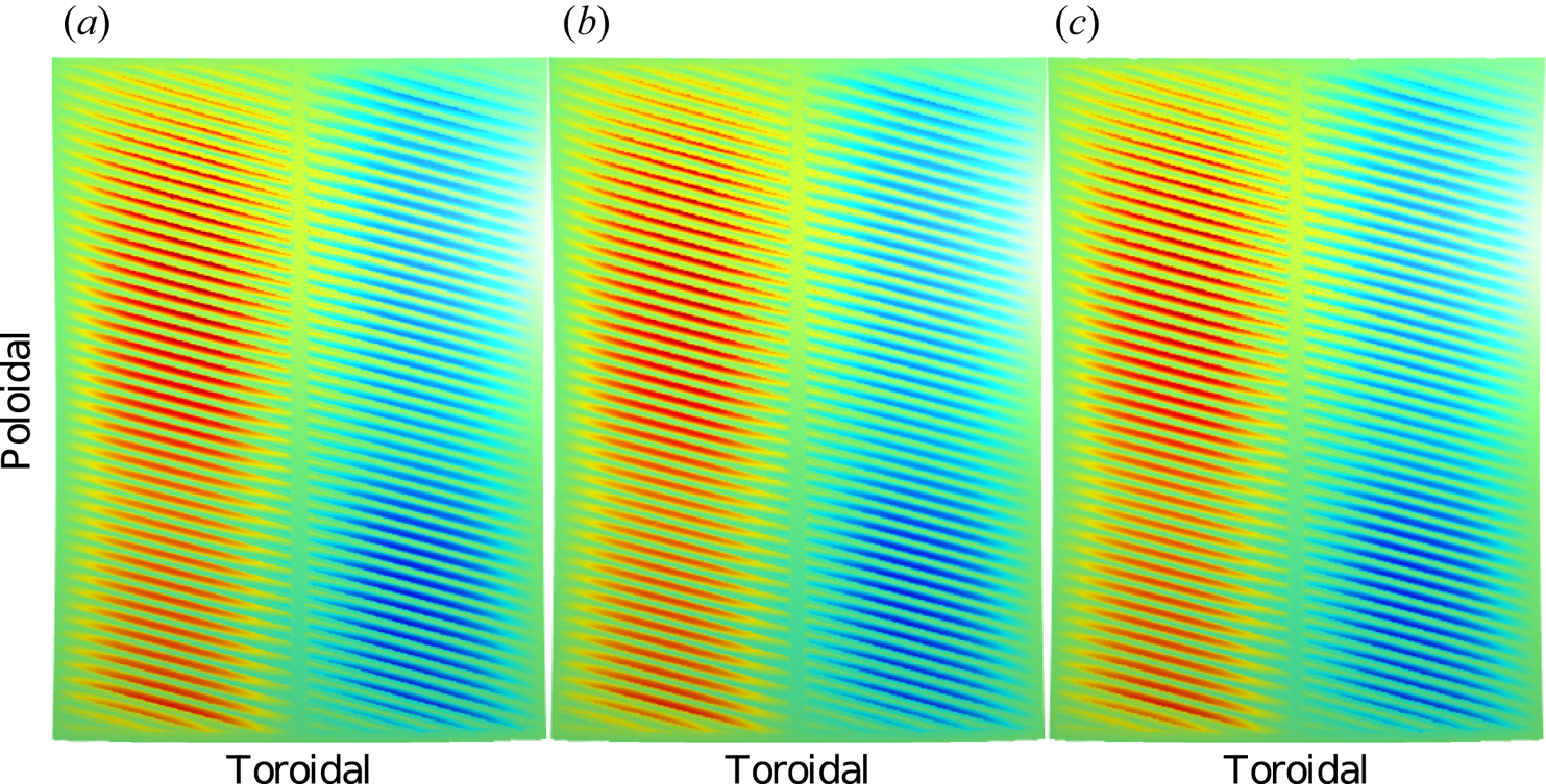
Poloidal tangential electric field component along the plasma–vacuum interface in a RAPLICASOL calculation of the ASDEX Upgrade 2-strap antenna, with the interface meshed with a typical mesh size of 5 cm (a), 3 cm (b) and 1 cm (c). The main toroidal asymmetry is due to the dipole phasing of the antenna. Convergence cannot be reached: the denser we mesh the interface, the shorter-wavelength surface wave modes become available in the near-nullspace of the nearly singular finite element matrix.
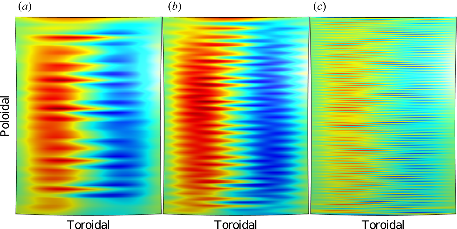
This non-convergence is not seen on one-dimensional interfaces in two-dimensional calculations, such as those shown in figure 6: at fixed $k_z$ , surface waves of arbitrarily short wavelength do not exist.
Although concerning, this lack of convergence is not as great a problem as it might appear at first sight. After all, despite being non-converged, these codes have made quantitatively correct predictions of ICRF physics (Tierens et al. Reference Tierens, Milanesio, Urbanczyk, Helou, Bobkov, Noterdaeme, Colas and Maggiora2019; López et al. Reference López, Cianciosa, Lunt, Tierens, Bilato, Birkenmeier, Bobkov, Dunne, Ochoukov and Strumberger2020). Since the surface waves decay in both directions away from the interface, and the shorter-wavelength ones decay faster, quantities of interest evaluated far enough away from the interface are likely to have negligible contributions from the surface waves. Usually, we are interested mainly in the following.
(i) On the vacuum side, the electric fields in or very near the antenna, for near-field modelling, sheath physics and suppression of impurity production (Tierens et al. Reference Tierens, Jacquot, Bobkov, Noterdaeme and Colas2017). The aperture is typically several centimetres away from the plasma–vacuum interface. Figure 9 shows that the fields at the aperture in ASDEX Upgrade antenna calculations are not appreciably affected by the surface waves.
(ii) On the plasma side, the power the antenna is able to couple to the plasma. From the point of view of a finite element code, this is the power absorbed in the PMLs, but it is typically calculated via the S-matrix, a quantity that depends solely on the fields in the ports, much further away from the plasma–vacuum interface than the aperture, and thus much less affected by the surface waves. Thus, if we believe the fields at the aperture to be converged, we should also expect the S-matrix, and thus the coupled power, to be converged.
Poloidal tangential electric field component along the antenna aperture, for the cases from figure 8. The antenna aperture is on the vacuum side of the plasma–vacuum interface, about 3 cm away from the interface. Despite the non-convergence of the fields on the plasma–vacuum interface in figure 8, the fields on the aperture show no signs of non-convergence. The main toroidal asymmetry is due to the dipole phasing of the antenna. The main poloidal pattern is due to the nearby Faraday screen bars, which are about 5 cm away from the plasma–vacuum interface.
The upper bound for the vacuum decay length of the surface waves (5.14) provides a safe estimate for how far from the plasma–vacuum interface we must evaluate field quantities to be confident that they are not polluted by non-converged surface waves, but it overestimates the radial length scales of the surface waves actually observed in calculations. For example, (5.14) predicts a decay length of at most 0.6 m for a vacuum–plasma density jump of $10^{17}$ m$^{-3}$
 under typical ASDEX Upgrade conditions, even though we see from figure 9 that a few centimetres is in practice sufficient. If surface waves are excited at all, a lower bound for the vacuum decay length occurs at the shortest resolvable poloidal wavelength, $k_y=-{\rm \pi} /\varDelta _y$
 , given by the poloidal mesh size $\varDelta _y$
 . Using the asymptotes of (5.12) at large negative $k_y$
 , the shortest possible vacuum decay length is approximately

which gives respectively 1.6 and 1 cm and 3 mm for the cases of figures 8 and 9. Heuristically, one should evaluate field quantities ideally at least the maximum length scale (5.14) away from the plasma–vacuum interface, which is actually realistic for the fields in the ports and the S-matrix, but failing that, one should ensure to be at least several times the minimum length scale (7.3) away.
Physically, surface wave amplitudes are always limited by loss mechanisms, which include the inherent collisionality of the edge plasma, the eventual coupling of the surface wave's constituent evanescent wave modes to propagating waves (i.e. the wave modes are locally evanescent near the interface, but not globally evanescent as in § 2) or edge loss mechanisms like sheath rectification. Such loss mechanisms limit the surface wave amplitude, but also broaden the ‘resonance’ peaks: where in the lossless case, we have unconstrained amplitudes only on specific one-dimensional curves in ($k_y,k_z$ ) space, in the lossy case, the amplitudes remain finite, but also points near the resonant curve in ($k_y,k_z$
 ) space are affected.
8. Conclusion
In this work we derived both exact and approximate dispersion relations for surface waves on discontinuous interfaces between anisotropic media, in particular between vacuum and magnetized plasma. Due to the anisotropic nature of the magnetized plasma, surface waves exist even where they would not be expected classically; in particular, a sign change of $\boldsymbol {\epsilon }_{11}$ is not necessary.
We focused on the case of steep density gradients, which is the case most relevant for ICRF, but the techniques developed in this work are not limited to that case. Surface waves at any material parameter discontinuity, including sudden changes in the direction of anisotropy, such as those predicted by Dyakonov (Reference Dyakonov1988) in uniaxial crystals, can be described using these techniques.
In numerical ICRF calculations, it is common to use discontinuous plasma–vacuum interfaces as a simple way of avoiding issues associated with the lower hybrid resonance. This common trick is not without its side effects: non-physical surface waves form, which cannot be absorbed by PMLs (§ 6) and prevent convergence (§ 7). It is certainly possible to suppress such surface wave excitation by introducing losses. The effects of such interventions, and whether a PML variant can be formulated that absorbs all the surface waves and all the bulk waves, remain open questions.
We derived first-order corrections to these dispersion relations for physical surface waves on steep but continuous material interfaces, which provides a qualitative explanation of steepness-dependent surface wave behaviour that has been observed in finite element calculations.
Acknowledgements
We acknowledge fruitful discussions with S. Shiraiwa and N. Bertelli (PPPL), and R. Bilato and M. Usoltceva (IPP Garching). This work has been carried out within the framework of the EUROfusion Consortium and has received funding from the Euratom research and training programme 2014–2018 and 2019–2020 under grant agreement no. 633053. The views and opinions expressed herein do not necessarily reflect those of the European Commission.
Editor Per Helander thanks the referees for their advice in evaluating this article.
Declaration of interests
The authors report no conflict of interest.
Appendix A. Asymptotics for the Laplace-transformed electric field in a medium with exponentially varying permittivity
Theorem A.1 Let $\boldsymbol {e}(x)$ be a solution on $x\in [0,\infty [$
 of the wave equation with given $k_y,k_z$
 :
:

where $\boldsymbol {\epsilon }(x)=\boldsymbol {\epsilon }_1+\boldsymbol {\epsilon }_2\exp (-\alpha x)$ , with $\boldsymbol {\epsilon }_1, \boldsymbol {\epsilon }_2$
 either constant scalars or constant $3\times 3$
 matrices, and $\alpha >0$
 . The four boundary conditions for $\boldsymbol {e}(x)$
 are specified values for $e_y(0),e_y'(0), e_z(0),e_z'(0)$
 which do not depend on $\alpha$
 .
.
Then
(i) The $n$
th derivative $e_x^{(n)}(0)$ is an $n$th-degree polynomial in $\alpha$.(ii) The $(n+1)$
th derivatives $e_y^{(n+1)}(0)$ and $e_z^{(n+1)}(0)$ are $n$th-degree polynomials in $\alpha$.


Proof. By induction. At $n=0$ , it is clearly the case that $e_y^{(0+1)}(0)$
 and $e_z^{(0+1)}(0)$
 are zeroth-order polynomials, i.e. constants, since these are two of the boundary conditions which by assumption do not depend on $\alpha$
 . It is also the case that $e_x^{(0)}(0)$
 is constant, its value being given by (4.8).
For the induction step: suppose $e_x^{(k)}(0)$ , $e_y^{(k+1)}(0)$
 and $e_z^{(k+1)}(0)$
 are indeed $k$
 th-order polynomials in $\alpha$
 , for all $k$
 up to $k=n$
 . Take the $(n+1)$
 th derivative of the $x$
 component, and the $n$
 th derivative of the $y$
 and $z$
 components, of the wave equation:

Explicitly,


Note that, by the induction hypothesis, the right-hand side has an $(n+1)$ th-degree polynomial in $\alpha$
 on the first row and an $n$
 th-degree polynomial in $\alpha$
 on the second and third rows. The second term on the left-hand side is a polynomial in $\alpha$
 of at most $n$
 th degree. Thus, $e_x^{(n+1)}(0), e_y^{(n+2)}(0), e_z^{(n+2)}(0)$
 must be polynomials in $\alpha$
 of degree $n+1$
 .
.
Theorem A.2 Let $\boldsymbol {e}(x)$ be defined as in Theorem A.1. Let $C_{\alpha }^{n}(P)$
 be the coefficient of $\alpha ^{n}$
 in the polynomial $P$
 . Then for all $n>0$
 , $C_{\alpha }^{n}(e_x^{(n)}(0))$
 obeys the recurrence relation

with boundary condition

given by (4.8).
Proof. Consider the second and third row of (A3). There are only two terms in $\alpha ^{n+1}$ in each row. In the second row, there is one due to $e_x^{(n+1)}(0)$
 and one due to $e_y^{(n+2)}(0)$
 . In the third row, there is one due to $e_x^{(n+1)}(0)$
 and one due to $e_z^{(n+2)}(0)$
 . The second and third rows on the right-hand side are of degree at most $n$
 in $\alpha$
 . Thus,


Consider now the first row of (A3):


The left-hand side is clearly 0, so

By Theorem A.1, only $C_{\alpha }^{n+1}(e_x^{(n+1)}(0))$ can be non-zero; $C_{\alpha }^{n+1}(e_y^{(n+1)}(0))$
 and $C_{\alpha }^{n+1}(e_z^{(n+1)}(0))$
 must both be zero, so

To simplify, replace $n$ by $n-1$
 , and move the $\boldsymbol {\epsilon }_{2,11} C_{\alpha }^{n}(e_x^{(n)}(0))$
 and $\boldsymbol {\epsilon }_{2,11} e_x(0)$
 terms into the sum:

which is (A5).
Theorem A.3 For isotropic media, the last term in (A5) disappears. The solutions of the resulting homogeneous recursion relation

are

where $A_n$ is the so-called Eulerian polynomial of $n$
 th degree (see Hirzebruch (Reference Hirzebruch2008) for details), which can be defined by


Proof. Let us start from (A17). Multiplying both sides by $(t-1)^{-n}$ :
:

Adding and subtracting the $k=n$ term on the right-hand side:


Multiplying both sides by $(-1)^{n}$ :
:

Let ${1}/{t}=-({\boldsymbol {\epsilon }_{2,11}}/{\boldsymbol {\epsilon }_{1,11}})$ and $C_{\alpha }^{n}(e^{(n)}_x(0))= A_n(t) (1-t)^{-n}$
 , then (A22) is (A14).
Theorem A.4 The solution of the full inhomogeneous recurrence relation (A5) with boundary condition (A6) is explicitly

with

Proof. Using Theorem A.3, (A23) clearly obeys

Thus

which is (A5) if

which is (A24).
Theorem A.5 Let $\boldsymbol {e}(x)$ be defined as in Theorem A.1, and let ${\boldsymbol {\epsilon }_{2,11}}/{\boldsymbol {\epsilon }_{1,11}}>-1$
 , such that $\boldsymbol {\epsilon }_{11}(x)=\boldsymbol {\epsilon }_{1,11}+\boldsymbol {\epsilon }_{2,11}\exp (-\alpha x)$
 has no roots at positive $x$
 . Then the Laplace-transformed electric field,

is asymptotically, at high $\alpha$ ,
,


for any constant $s_0$ , and $\phi$
 defined as in (A24).
Proof. Both $\boldsymbol {e}(x)$ and $\boldsymbol {E}(s)$
 depend, in general, on $\alpha$
 . Let us make this dependence explicit:

Suppose $\boldsymbol {e}(x,\alpha )$ can be expressed in a Taylor series in $x$
 near the origin:


Suppose that in the high-$\alpha$ limit, the integral is some constant $K$
 :
:

Then

For $e_y$ and $e_z$
 , we know from Theorem A.1 that $e_{y\text { or }z}^{(n)}(0,\alpha )$
 grows at most as fast as $\alpha ^{n-1}$
 (with the $n=0$
 and $n=1$
 terms both constant), so only the $n=0$
 term remains in the limit


(it does not depend on $\alpha$ , since $e_y(0)$
 and $e_z(0)$
 are boundary conditions). Thus,


The situation is more complicated for $E_x$ , where the higher terms do not disappear in the high-$\alpha$
 limit. Instead,

We know the terms $C_{\alpha }^{n}(e_x^{(n)}(0,\alpha ))$ from Theorem A.4:

Hirzebruch (Reference Hirzebruch2008) shows the Eulerian polynomials $A_n(t)$ have the exponential generating function

which lets us work out (A42) explicitly:


which gives us (A29).
Note that the integral (A45) diverges when ${\boldsymbol {\epsilon }_{2,11}}/{\boldsymbol {\epsilon }_{1,11}}<-1$ , that is, when $\boldsymbol {\epsilon }_{11}(x)=\boldsymbol {\epsilon }_{1,11}+\boldsymbol {\epsilon }_{2,11}\exp (-\alpha x)=0$
 at some $x>0$
 , when a resonance might occur. The function $(1+{\boldsymbol {\epsilon }_{1,11}}/{\boldsymbol {\epsilon }_{2,11}}) \log (1+{\boldsymbol {\epsilon }_{2,11}}/{\boldsymbol {\epsilon }_{1,11}})$
 is well-behaved in ${\boldsymbol {\epsilon }_{2,11}}/{\boldsymbol {\epsilon }_{1,11}}\in [-1,\infty [$
 , with the $\boldsymbol {\epsilon }_{2,11}\rightarrow 0$
 limit being

The correctness of (A29) is further supported by numerical results in figure 10. To obtain this figure, we solved the wave equation (A1) numerically using Runge–Kutta methods over a finite range $x\in [0,x_{\text {max}}]$ with $x_{\text {max}}\gg 1/\alpha$
 , such that $x>x_{\text {max}} \implies \boldsymbol {\epsilon }(x)\approx \boldsymbol {\epsilon }_1$
 . Knowing that in $]x_{\text {max}},\infty [$
 the dielectric tensor is approximately constant, and the solution of the wave equation thus analytically known, we extend the solution analytically in $]x_{\text {max}},\infty [$
 , starting from the numerically determined values at $x_{\text {max}}$
 . We then calculate the Laplace transform via numerical integration in $[0,x_{\text {max}}]$
 , and analytic integration in $]x_{\text {max}},\infty [$
 .
.
Solid lines: numerical calculation of $\boldsymbol {E}(s_0+\alpha )$ (the Laplace-transformed electric field in a medium with $\boldsymbol {\epsilon }=\boldsymbol {\epsilon }_1+\boldsymbol {\epsilon }_2\exp (-\alpha x)$
 ) compared with the asymptotic expressions from Theorem A.5, which are the dashed lines. The left-hand panel shows an isotropic case and the right-hand panel an anisotropic case. Parameters for the left-hand panel are ${\omega }/{c}=1$
 m$^{-1}$
 , $\boldsymbol {\epsilon }_1=1,\boldsymbol {\epsilon }_2=2$
 , $k_y=1$
 , $k_z=2$
 , $s_0=9$
 m$^{-1}$
 . Parameters for the right-hand panel are ${\omega }/{c}=1$
 m$^{-1}$
 , $\boldsymbol {\epsilon }_1=\left [\begin{smallmatrix} 1 & -\textrm {i}/2 & 0 \\ \textrm {i}/2 & 1 & 0 \\ 0 & 0 & 10 \end{smallmatrix}\right ],\ \boldsymbol {\epsilon }_2=\left [\begin{smallmatrix} 1/4 & -2 \textrm {i} & 0 \\ 2 \textrm {i} & 1/4 & 0 \\ 0 & 0 & 3 \end{smallmatrix}\right ]$
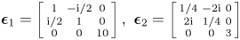 , $k_y=1$
 , $k_z=2$
 , $s_0=9$
 m$^{-1}$
 . For both panels, the boundary conditions are $e_y(0)=1$
 , $e_z(0)=0.5$
 V m$^{-1}$
 , $e_y'(0)=0$
 , $e_z'(0)=0$
 V m$^{-2}$
 .
.

Appendix B. Assessing ‘wave forwardness’ graphically from the shape of the dispersion curves at constant $\omega$ in $\boldsymbol {k}$ space


The dispersion relation is

The group velocity is

From the gradient in the numerator of (B2), we see that the group velocity is everywhere perpendicular to the dispersion relation in $(k_x,k_y)$ space.
The ‘wave forwardness’ in the $y$ and $z$
 directions then depends, respectively, on the sign of

and

The wave is forward in one of the two directions and backward in the other if the signs of (B3) and (B4) are opposite, i.e.

Now

Thus, a problem of wave backwardness arises in either direction when


This property may be easily assessed graphically from the shapes of the dispersion curves. Considering dispersion curves at different frequencies is only necessary to know in which of the two directions, $y$ or $z$
 , the wave is backward.


 Open access