


1. Introduction
Internal solitary waves (ISWs) are widely observed in coastal oceans as well as lakes (Helfrich & Melville Reference Helfrich and Melville2006; Lamb Reference Lamb2014; Boegman & Stastna Reference Boegman and Stastna2019). Notable study sites include the South China Sea (Chang et al. Reference Chang, Lien, Lamb and Diamessis2021), the Strait of Gibraltar (Alpers, Brandt & Rubino Reference Alpers, Brandt, Rubino, Gade and Barale2008) and the New Jersey Shelf (Shroyer, Moum & Nash Reference Shroyer, Moum and Nash2009). These waves can propagate without changing form over hundreds of kilometres, and thus provide a coherent mechanism for both horizontal (Lamb Reference Lamb1997) and vertical transport of scalars (e.g. nutrients, pollutants) (Boegman & Stastna Reference Boegman and Stastna2019). The interaction of ISWs with the bottom boundary layer has been documented in the field (Bogucki, Dickey & Redekopp Reference Bogucki, Dickey and Redekopp1997), in laboratory experiments (Carr, Davies & Shivaram Reference Carr, Davies and Shivaram2008; Grue & Sveen Reference Grue and Sveen2010) and in simulations (Diamessis & Redekopp Reference Diamessis and Redekopp2006; Aghsaee, Boegman & Lamb Reference Aghsaee, Boegman and Lamb2010). When the bottom is flat, ISWs of depression (waves for which isopycnals are depressed from their rest height) have been found to induce a prograde jet in the bottom boundary layer that trails the main wave. It is this jet that can undergo a vortex-forming instability (Sakai, Diamessis & Jacobs Reference Sakai, Diamessis and Jacobs2020). However, the reconciliation between simulations and an experimental instability threshold has been established only recently (Ellevold & Grue Reference Ellevold and Grue2023) and only using two-dimensional simulations.
In the field, most ISWs eventually propagate into shallower waters, transforming during the shoaling process. The slopes reported in the field are quite small, with  $s=\tan \theta \approx 0.01\unicode{x2013}0.03$ being typical (Boegman & Stastna Reference Boegman and Stastna2019). For ISWs of depression, the shoaling process leads to a broadening of the front, and steepening of the rear of the wave. The prograde jet experiences a horizontal ‘pinching’, that yields a localised separation bubble beneath the rear face of the wave. This separation bubble evolves in a dynamic environment, especially when waves reach the so-called turning point, and begin to transform from an ISW of depression into a train of waves of elevation. In terms of the broadly accepted characterisation of shoaling processes, the above described process is referred to as the ‘fissioning regime’, and has been successfully simulated to date only in two dimensions (Xu & Stastna Reference Xu and Stastna2020). Shoaling experiments initialised with an elevated pycnocline have also been observed to result in similarly structured wave trains that result in strong surges of along-shore currents (Grue & Sveen Reference Grue and Sveen2010).
The concept of separation bubbles has its origin in aerodynamics (Lin & Pauley Reference Lin and Pauley1996), e.g. on the rear portion of aerofoils, and instability mechanisms, as well as aspects of fully three-dimensionalised behaviour, are well known to depend on the strength of the counter-flow within the separation bubble and the bubble length (Alam & Sandham Reference Alam and Sandham2000; Rodríguez, Gennaro & Juniper Reference Rodríguez, Gennaro and Juniper2013). Shoaling ISWs in the fissioning regime provide an environment that is partially analogous to the aerofoil case, but only to a certain degree since the basic background state (e.g. the wavetrain) is evolving. To date, it has thus been an open question as to how shoaling ISWs in the fissioning regime induce three-dimensionalisation. We report on three-dimensional simulations of ISWs generated via lock release in a tilted laboratory scale tank, carried out with a well-validated pseudo-spectral code. The ISWs form, transform and pass through the turning point, eventually transforming into a train of up-slope moving boluses. We identify episodes of three-dimensionalisation, finding that while separation bubbles do contribute to three-dimensionalisation, it is the bolus generating stage that is the most consistent source of three-dimensionalisation (consistent with both field Richards et al. (Reference Richards, Bourgault, Galbraith, Hay and Kelley2013) and laboratory Ghassemi, Zahedi & Boegman (Reference Ghassemi, Zahedi and Boegman2022) measurements). We conclude with a discussion of similarities and differences with the three-dimensionalisation of aerodynamic separation bubbles, and with a discussion on how shallow-shoaling waves may inject sediment into the water column without the inviscid breaking mechanisms typical of waves shoaling over steep slopes.
2. Methodology
2.1. The governing equations and system configuration
We investigate shoaling by simulating a lock-release experiment in a rectilinear tank tilted at angle  $\theta$ from horizontal of the lab frame of reference. The tank is tilted as illustrated in figure 1. Thus in the frame of the tilted tank (the solid black box in figure 1), the acceleration due to gravity is given by
 \begin{equation} \boldsymbol{g} ={-}g(\sin\theta,0,\cos\theta), \end{equation}
where  $g=9.81$ m s $^{-2}$.
A schematic of the initial conditions. The region between the red and blue curves represents the pycnocline, and the black curve represents the contour  $\rho /\rho _0 = 1$. Note that the $y$-axis is assumed to point into the page, and that $L_y$ (not in the diagram) will denote the spanwise width of the domain.

We implement the tilted-tank lock-release using the initial conditions
 \begin{gather} \frac{\rho}{\rho_0} = 1 - \frac{\Delta\rho}{2}\tanh \left\{\frac{z\cos\theta+x\sin\theta-H\exp\left(\dfrac{-x^2}{L_w^2}\right)-z_0}{h}\right\}, \end{gather}
 \begin{gather}\boldsymbol{u} = \phi_p \boldsymbol{\varXi}. \end{gather}
Equation (2.2) represents a quasi-two-layer stratification, where the initial perturbation of the pycnocline has a Gaussian profile with amplitude  $H$ and width $L_w$; the thickness of the pycnocline is given by $h$, and the non-dimensional density difference between the upper and lower layers is given by $\Delta \rho$. The height of the undisturbed pycnocline is $z_0$, chosen so that it is above mid-depth near the left boundary, and below mid-depth where it intersects the sloped bottom boundary. (Note that mid-depth is measured from $z=0$ and along $-\boldsymbol {g}/g = (\sin \theta,0,\cos \theta )$.) See figure 1 for an illustration of (2.2), and table 1 for the numerical values of these parameters (all constant with the exception of $H$, which is varied as part of the numerical experiments described in § 2.2). Equation (2.2) is written using coordinates measured in the frame of the tilted tank, $(x,y,z)$; we take the streamwise direction to point along the $x$-axis, spanwise along the $y$-axis, and vertical along the $z$-axis (see figure 1). The coordinates in the lab frame are given by
 \begin{equation} \begin{pmatrix} \hat{x} \\ \hat{y} \\ \hat{z} \end{pmatrix}=\begin{pmatrix} \cos\theta & 0 & -\sin\theta \\ 0 & 1 & 0 \\ \sin\theta & 0 & \cos\theta \end{pmatrix} \begin{pmatrix} x \\ y \\ z \end{pmatrix}. \end{equation}
Note that components of vectors and tensors measured in the lab frame will also be denoted by symbols with a circumflex. In (2.3),  $\phi _p=10^{-3}$ m s $^{-1}$, and $\boldsymbol {\varXi }$ is a vector of dimensionless random variables that follows a normal distribution with mean $0$ and standard deviation $1$. This means that the fluid is initially at rest to leading order, with a small stochastic perturbation that instigates hydrodynamic instabilities.


We evolve the initial conditions described by (2.2) and (2.3) using the incompressible, stratified Navier–Stokes equations under the Boussinesq approximation. Derivations of the equations and Boussinesq approximation can be found in Kundu & Cohen (Reference Kundu and Cohen2004) and Batchelor (Reference Batchelor2000):
 \begin{gather} \boldsymbol{\nabla}\boldsymbol{\cdot}\boldsymbol{u} = 0, \end{gather}
 \begin{gather}\frac{{\rm D}{\boldsymbol{u}}}{{\rm D} t} ={-}\frac{1}{\rho_0}\,\boldsymbol{\nabla} P + \frac{\rho}{\rho_0}\,\boldsymbol{g}+\nu\,\nabla^2\boldsymbol{u}, \end{gather}
 \begin{gather}\frac{{\rm D}{\rho}}{{\rm D} t} = \kappa\,\nabla^2\rho. \end{gather}
In the above set of equations,  $\boldsymbol {u}$ is the fluid velocity, $\rho _0$ is a constant reference density, $\rho$ is the deviation of the density from the constant reference density, $\boldsymbol {g}$ is the acceleration due to gravity (the components of $\boldsymbol {g}$ are given by (2.1) in the tilted frame, and $(0,0,-g)$ in the lab frame), $\nu$ is the kinematic viscosity, and $\kappa$ is the scalar diffusivity.
We assume free-slip boundary conditions along the streamwise-normal and spanwise-normal boundaries, and – due to our interest in boundary layer instabilities – assume no-slip boundary conditions along the upper and lower boundaries. We assume no-flux boundary conditions for  $\rho$. The domain dimensions are $L_x \times L_y \times L_z=8.192\,\text {m} \times 0.256\,\text {m} \times 0.300\,\text {m}$, and the grid size is $N_x \times N_y \times N_z = 8192 \times 256 \times 256$; this gives resolution $1.00\,\text {mm} \times 1.00\,\text {mm} \times 1.18\,\text {mm}$. Numerical solutions are produced using SPINS, an MPI-parallelised pseudo-spectral solver (Subich, Lamb & Stastna Reference Subich, Lamb and Stastna2013).
2.2. The numerical experiments and quantities of interest
Our experiments involve varying the amplitude  $H$ of the initial disturbance given by (2.2). The case with the smallest amplitude is labelled ‘S’, with the medium amplitude labelled ‘M’, and the large amplitude labelled ‘L’. In the following, all reported quantities have been non-dimensionalised.
We use  $\mathcal {L} = z_0$ as the characteristic length. For our characteristic speed, we choose the amplitude-dependent $\mathcal {U}=c_{NL}$, where
 \begin{gather} c_{NL} = c_{\text{lw}}+\alpha H, \end{gather}
 \begin{gather}c_{lw} = \sqrt{g\,\Delta\rho\,\frac{h_1h_2}{h_1+h_2}}, \end{gather}
 \begin{gather}\alpha = \frac{3}{2}\,c_{lw}\,\frac{h_1-h_2}{h_1h_2}, \end{gather}
and  $h_1$ and $h_2$ are the the thicknesses of the upper and lower layers. Given that we use a sloped domain, we make following estimates (Xu & Stastna Reference Xu and Stastna2020):
 \begin{gather} h_1 = \frac{z_0+L_z/2}{2}, \end{gather}
 \begin{gather}h_2 = L_z-h_1. \end{gather}
The expressions in (2.9) and (2.10) are derived from Korteweg–de Vries (KdV) theory by assuming idealised vertical structure functions and applying the Fredholm alternative to the standard KdV equation as outlined in Stastna (Reference Stastna2022). Furthermore, (2.8) follows the form of the nonlinear advection speed in the KdV equation (Stastna Reference Stastna2022).
Using  $\mathcal {L}$ and $\mathcal {U}$, we can then compute our characteristic time as
 \begin{equation} T = \frac{z_0}{c_{NL}}, \end{equation}
which varies across cases. While several choices of non-dimensionalisation exist in the literature (see Aghsaee et al. Reference Aghsaee, Boegman and Lamb2010; Boegman & Stastna Reference Boegman and Stastna2019; Xu & Stastna Reference Xu and Stastna2020), our choices of characteristic scales will allow us to collapse the timing of when the systems are maximally three-dimensional.
Our study concerns the interaction of phenomena on disparate scales; namely, we study the interaction between a large-amplitude shoaling wave and a thin bottom boundary layer. The shoaling wave is characterised by the wave Reynolds number, which uses the (initial) wave amplitude  $H$ as the length scale, instead of $z_0$ (Xu & Stastna Reference Xu and Stastna2020):
 \begin{equation} Re = \frac{c_{NL}H}{\nu}. \end{equation}
We estimate/characterise the height of the boundary layer using the Stokes boundary layer thickness (Arthur & Fringer Reference Arthur and Fringer2014)
 \begin{equation} \delta = 2\sqrt{\frac{\nu L_w}{c_{NL}}}. \end{equation}
The quantities defined above vary in each case, and their values are collected in table 2.
The experimental parameters.

Our systems transition from two-dimensional to three-dimensional flow after the onset of certain instabilities. As such, we need to individually characterise the three-dimensional and two-dimensional motions. An immediate method to do so is to compare the streamwise and spanwise stresses generated on the bottom boundary. As will be discussed in § 3.3, the former indicates when the separation bubble ‘bursts’, while the latter indicates the presence of three-dimensional motion. The bed stresses are given by the non-dimensional form
 \begin{equation} \tau_{x_i} = \left.\frac{\nu}{c_{NL}^2}\,\frac{\partial{u_i}}{\partial{z}}\right|_{z=0}, \end{equation}
where  $i=1,2$, and $x_1=x$ and $x_2=y$. More specifically, we consider the $L_2$-norm of the stresses:
 \begin{equation} L_2(\tau_{x_i}) = \sqrt{\frac{z_0^2}{L_xL_y}\int_{0}^{L_{y}/z_0} \int_{0}^{L_{x}/z_0}\tau_{x_i}^2(x,y,t)\,\text{d}\kern0.06em x\,\text{d}y}. \end{equation}
A second method to characterise the flow is to follow the example of Caulfield & Peltier (Reference Caulfield and Peltier2000) and decompose the velocity field into a two-dimensional (2-D) background and a three-dimensional (3-D) perturbation:
 \begin{gather} \boldsymbol{u}^{{2\text{-}D}} = (\langle u \rangle_{y},0,\langle w \rangle_{y}), \end{gather}
 \begin{gather}\boldsymbol{u}^{{3\text{-}D}} = (u-\langle u \rangle_{y},v,w-\langle w \rangle_{y}), \end{gather}
where  $\langle {\,\cdot\,} \rangle _{y}$ denotes an average in the spanwise direction. Note that this decomposition and the spanwise average are performed in the frame of the tilted tank. We will compare the domain average of the resultant two- and three-dimensional kinetic energies, which are given respectively by
 \begin{gather} \text{KE}^{{2\text{-}D}} = \left\langle \tfrac{1}{2}((u^{{2\text{-}D}})^2+(w^{{2\text{-}D}})^2)\right\rangle_{xyz}, \end{gather}
 \begin{gather}\text{KE}^{{3\text{-}D}} = \left\langle\tfrac{1}{2}((u^{{3\text{-}D}})^2+(v^{{3\text{-}D}})^2+(w^{{3\text{-}D}})^2)\right\rangle_{xyz}, \end{gather}
where  $\langle {\,\cdot\,} \rangle _{xyz}$ denotes the domain average.
We will also analyse the domain-averaged rate of viscous dissipation (Wyngaard Reference Wyngaard2010),
 \begin{equation} \epsilon = \left\langle \frac{2H/z_0}{Re}\,S_{ij}S_{ij}\right\rangle_{xyz}, \end{equation}
where  $S_{ij}$ is the symmetric part of the velocity gradient tensor. Viscous dissipation will be generated by both friction at the boundaries induced by the shoaling wave, and highly unstable flow in the water column induced by boundary layer instabilities. Large concurrent peaks in viscous dissipation and kinetic energy are indicative of a quasi-turbulent flow (Wyngaard Reference Wyngaard2010).
3. Results of the numerical experiments
3.1. Three-dimensionalisation due to the separation bubble and interaction with the pycnocline
Initially, our systems closely resemble the two-dimensional simulations of Xu & Stastna (Reference Xu and Stastna2020) (see their figure 2). A region of retrograde flow grows out of the boundary layer under the large prograde separation bubble beneath the first wave of elevation; we highlight these with grey boxes in figures 2(a,b). The formation of the retrograde region within the prograde separation bubble results in the formation of a vortex that drifts leftwards and eventually exits the separation bubble for systems with a sufficiently high  $Re$. We will refer to this event as the ‘bursting’ of the separation bubble. After the bubble ‘bursts’, new retrograde regions form and in turn shed more vortices. In our M and L cases, we observe bursting, while in our case S (characterised by having the smallest $H$ and $Re$), we do not observe bursting, as any vortex generated by a region of retrograde flow is extinguished before it can exit the prograde separation bubble. The formation of retrograde bubbles and the shedding of vortices is a dynamic process, and the present discussion is augmented by movies 1, 2 and 3 in the supplementary material (available at https://doi.org/10.1017/jfm.2024.703).
A comparison of the lab-frame velocity components of cases M and L at  $t \approx 41$, a time by which cases M and L have undergone at least one bursting event: (a,c,e) case M, and (b,d,f) case L. (a,b) The streamwise velocity field sampled at $\hat {y}=L_y/(2 z_0)$. (c,d) The spanwise velocity field sampled at $\hat {y}=L_y/(2 z_0)$. (e,f) The vertical velocity field sampled at $z=\delta /z_0$ (as the boundary layer thickness is measured normal to the bottom boundary). Note that (a,b) also contain contours of $\rho = 1$ in the plane $y=L_y/(2 z_0)$. The dashed horizontal line $\hat {z}=z_0$ indicates the position of the pycnocline if it were undisturbed. Black rectangles in (a,b) highlight vortices shed by the bursting separation bubble. A double-headed arrow pointing between (b) and (d) highlights the transverse flow generated by the vortex shed by the bubble in case L. Note that the windows in all plots have dimensions $6\times 1$, though the axes do not use the same scales.

The shed vortices correspond to localised regions of shear under the pycnocline in the  $\hat {u}$ field; examples of these are indicated by black boxes in figure 2(a) (case M) and figure 2(b) (case L), where we visualise the velocity components. At this time, case L has undergone two bursting events, while case M is undergoing its first. In figures 2(a,b), we see vortices entrain the pycnocline, which is visualised with a black contour line. The vortex from case L is in the middle of overturning the pycnocline, and the vortex from case M is beginning this process. Finally, comparing figures 2(c,d), we see that the vortices in case L induce spanwise currents, while the case M vortex does not at this time. Indeed, comparing figures 2(e,f), we see that $w$ at the top of the boundary layer shows spanwise variation only in case L. As mentioned, case S never undergoes a bursting event, so is omitted from this figure.
In every case, the systems do eventually become three-dimensional, as can be seen in figure 3. This figure is formatted similarly to figure 2, but data from case S are included, and the fields are instead sampled at the time where KE $^{{3\text {-}D}}$ is at its maximum value; this time is $t=50.4$ for case S, $t = 49.6$ for case M, and $t = 48.0$ for case L. Notice that our choice of characteristic time (see (2.13)) has approximately collapsed the timing of this event across cases. The spatial distribution of three-dimensional structure varies between the cases. Figures 3(f,i) indicate that spanwise structure fills a continuous region between $\hat {x}=9$ and $\hat {x}=14$ (underneath the first and second waves of elevation) in case L. This is not so for case M: a black box in figure 3(h) highlights a region of two-dimensional structure separating two regions with three-dimensional flow. By $t=49.6$, case M has undergone three bursting events, and the spatial separation is a consequence of the vortices from the first, second and third bursting events inducing three-dimensional currents simultaneously, even though they were generated at separate times. In contrast, vortices shed by the separation bubble in case L induce three-dimensional currents immediately, and there is no spacing between the sources of three-dimensional flow, and therefore no possibility for the existence of interstitial regions with purely two-dimensional flow.
Similar to figure 2 but (i) at the time of the maximum KE $^{{3D}}$ for each case, and (ii) also including data from case S. The time of peak KE $^{\text{3-D}}$ is (a,d,g) $t=50.4$ for case S, (b,e,h) $t = 49.6$ for case M, and (c,f,g) $t = 48.0$ for case L. The grey rectangle in (a) shows a retrograde bubble bursting in the second wave of elevation from case S, and a black rectangle in (g) highlights the two-dimensional structure of the flow underneath this same wave. A black rectangle in (g) highlights a region of two-dimensional structure separating two regions with three-dimensional structure. Note that the windows in all plots have dimensions $7\times 1$, though the axes do not use the same scales.

Vortices in case S never induce spanwise structure: a grey box in figure 3(a) indicates a shed vortex and a retrograde bubble under the second wave of elevation, and the region highlighted by a black box in figure 3(g) shows that they are fully two-dimensional. The only three-dimensional structure is under the lead wave of elevation, which has become a bolus. This separate mechanism for the generation of spanwise currents is the topic of the next subsection.
3.2. Three-dimensionalisation of the flow within a bolus
The turning point is where the incident wave of depression fissions into a train of waves of elevation, and the attachment point is where the pycnocline intercepts the bottom boundary (Aghsaee et al. Reference Aghsaee, Boegman and Lamb2010; Arthur & Fringer Reference Arthur and Fringer2014; Nakayama et al. Reference Nakayama, Sato, Shimizu and Boegman2019). As the lead wave of elevation approaches the attachment point, it becomes a bolus. A bolus is distinguished from a wave of elevation, as it almost fully encloses a volume of fluid between the pycnocline and the bottom boundary, and thus more closely resembles a gravity current than a solitary wave; for a prototypical example, see figure 10 in Wallace & Wilkinson (Reference Wallace and Wilkinson1988). We observe that as the lead wave of elevation becomes a bolus, the prograde separation bubble fully occupies the region under the bolus, and it no longer produces internal retrograde separation bubbles.
It is during the transition from a wave of elevation to a bolus that another mechanism for three-dimensionalisation occurs. After passing the attachment point, the bolus develops a series of bulges and folds along its front, and a collection of billows along its top: these structures are due to the lobe-cleft instability and a shear instability, respectively (Simpson Reference Simpson1972). The lobe-cleft instability occurs when laterally intruding fluid rises over (or sinks under) lighter (denser) ambient fluid. Härtel, Carlsson & Thunblom (Reference Härtel, Carlsson and Thunblom2000) argue that it is an independent instability caused by the joint action of shear across, and an unstable density gradient under, the front of the lateral intrusion; recent numerical experiments link the initial spanwise structure of the lobe-cleft instability with the Rayleigh–Taylor instability (Xie, Tao & Zhang Reference Xie, Tao and Zhang2019). Lobes, clefts and billows have all been observed in boluses in numerical and experimental studies of shoaling waves, where they are observed to induce three-dimensional structure and the eventual degeneration of a bolus (Arthur & Fringer Reference Arthur and Fringer2014; Xu, Subich & Stastna Reference Xu, Subich and Stastna2016; Ghassemi et al. Reference Ghassemi, Zahedi and Boegman2022; Hartharn-Evans et al. Reference Hartharn-Evans, Carr, Stastna and Davies2022).
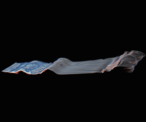
In figure 4, we present the pycnocline from case L at time  $t = 68.6$ and $12< x<19$. At this time, the lead wave of elevation is a bolus with structures formed by the aforementioned instabilities. The second wave of elevation is just beginning to transition into the bolus stage. Behind it, we see remaining disturbances in the pycnocline, which indicate sustained three-dimensional currents induced by the earlier bursting events. The lobe-cleft instability produces three-dimensional structure along the front of the current while inducing three-dimensional flow inside the current head via the action of hairpin vortices that extend from the front of the bolus and penetrate to the attachment point (Dai & Huang Reference Dai and Huang2022; Castro-Folker, Grace & Stastna Reference Castro-Folker, Grace and Stastna2023). In cases M and L, spanwise flow is trapped under waves of elevation as they become boluses. These currents initially decay, but persist long enough to eventually become energised by these hairpin vortices. Recall that none of the bursting events in case S induced spanwise flow, so the three-dimensional currents depicted in figures 3(d,g) are due entirely to the degeneration of the shear billows, and to the hairpin vortices produced by the lobe-cleft instability. Indeed, we can see the impressions left by the lobes at $\hat {x}=19.5$ in figure 3(g).
The pycnocline from case L at time  $t = 68.6$ and $12< x<19$. The opacity map sets regions where $\rho >1.005$ and $\rho <0.995$ to be transparent. Note that the bounds on the colour map do not correspond to the actual data range $0.99\leq \rho \leq 1.01$. At this time, the trailing wave of elevation becomes a bolus, while the lead wave/bolus takes the form of a gravity current with lobe-cleft and shear instabilities. Note that the lead wave has not yet passed the attachment point, but it has passed the point where the pycnocline intercepts the bottom boundary.

3.3. Quantitative measures of the onset and consequences of three-dimensionalisation
In figures 5(a,d), the formation of the retrograde region within the prograde separation bubble corresponds with first local maxima in the  $L_2(\tau _x)$ and $\epsilon$ signals, and we highlight this event in each case with a dashed vertical line in all plots. The formation of the retrograde region coincides with these maxima, as it causes the streamwise velocity component (measured in the tilted tank) to change its orientation (i.e. causes $u=0$) at multiple points within the boundary layer. This serves to decrease $L_2(\tau _x)$ and $\epsilon$ (which is dominated by friction at the no-slip boundaries prior to bursting).
A comparison of the stresses and energetics of the system: (a) the streamwise bed stress (see (2.17)); (b) the spanwise bed stress; (c) the ratio of the (domain-averaged) three-dimensional to two-dimensional kinetic energies (see (2.20) and (2.21)); and (d)) the domain-averaged rate of viscous dissipation (see (2.22)). In all plots, the dashed vertical lines (black corresponding to S, blue to M, and red to S) indicate the creation of an internal separation bubble, which coincides with the first instance of  $({\text {d}}/{\text {d}t})L_2(\tau _{x})= 0$ (i.e. the first local maximum in (a)).

For each case,  $L_2(\tau _x)$ and $\epsilon$ have subsequent local maxima, which are approximately concurrent with the global maximum of $L_2(\tau _y)$ and the first local maxima of $\text {KE}^{{3\text {-}D}}/\text {KE}^{{2\text {-}D}}$ in figures 5(b,c), respectively. Thus they are also approximately concurrent with the complex structures seen in figures 3(d–i), suggesting that vortices shed by bursting and lobe-cleft instabilities could both lead to quasi-turbulent states with the potential for sediment resuspension (Boegman & Stastna Reference Boegman and Stastna2019).
The vertical axis of figure 5(a) has a greater extent than that of figure 5(b), and the maximum value of KE $^{{3\text {-}D}}$/KE $^{{2\text {-}D}}$ across all cases is less than $0.14$. Additionally, the three-dimensional features in figures 3(g,h) are perturbations to vertical bars parallel to the $\hat {y}$-axis. Indeed, this is because the shoaling waves and the shed vortices advect the spanwise currents up or down the sloped domain. These facts indicate that the two-dimensional flow is the dominant feature of all systems. As will be discussed, this has implications for the extension of our results and the results of Xu & Stastna (Reference Xu and Stastna2020) to the field scale.
4. Discussion and conclusion
We have presented results from simulations of an internal solitary wave of depression shoaling over a realistic – and therefore shallow – slope. The shoaling wave fissions into a train of waves of elevation, which in turn become a train of boluses as the momentum of the waves pushes past the attachment point. We found that the shoaling wave induces two distinct instabilities at different phases of the shoaling process, and that both can induce three-dimensional structure in an initially two-dimensional system.
The first instability is a prograde separation bubble formed beneath the waves of elevation. The separation bubbles observed in aeronautics are contained within the boundary layer (Lin & Pauley Reference Lin and Pauley1996). In contrast, those formed beneath the shoaling internal wave extend much higher, even to the pycnocline (effectively a separation region rather than a ‘bubble’). The dynamics of this large region of prograde currents leads to the development of vortices that exit the separation region and travel towards the back of the domain in an event referred to as ‘bursting’ (Xu & Stastna Reference Xu and Stastna2020). The separation region continues to generate vortices after bursting. These vortices can induce three-dimensional instabilities, the growth rate of which depends on the wave amplitude, set by  $H$ in our configuration. We also observed that vortices shed by the M and L cases during bursting overturn the pycnocline. The process is less efficient for smaller waves, and in our case S no spanwise variation or pycnocline overturning was induced by bursting.
The second observed instability is the well-documented lobe-cleft instability (Simpson Reference Simpson1972; Härtel et al. Reference Härtel, Carlsson and Thunblom2000; Xie et al. Reference Xie, Tao and Zhang2019; Dai & Huang Reference Dai and Huang2022; Castro-Folker et al. Reference Castro-Folker, Grace and Stastna2023). Consistent with previous investigations (Arthur & Fringer Reference Arthur and Fringer2014; Xu et al. Reference Xu, Subich and Stastna2016; Ghassemi et al. Reference Ghassemi, Zahedi and Boegman2022; Hartharn-Evans et al. Reference Hartharn-Evans, Carr, Stastna and Davies2022), we observe that after a wave of elevation becomes a bolus, it develops folds and bulges along its front, and spanwise currents inside its head, due to shear and lobe-cleft instabilities. In contrast to the bursting of separation bubbles, the bolus approaching the attachment point led to three-dimensionalisation regardless of the initial wave amplitude. The boluses also developed shear instabilities along their tops, which further induced spanwise flow. Thus the bolus stage of the evolution led to three-dimensionalisation in every case, and can be expected to be the most abundant source of three-dimensionalisation for shallow-shoaling waves in the field (Richards et al. Reference Richards, Bourgault, Galbraith, Hay and Kelley2013).
Xu & Stastna (Reference Xu and Stastna2020) raised the question of whether or not three-dimensional flow would interrupt the bursting of the separation bubble and the overturning of the pycnocline, but here we see the exact opposite: it is only cases that can produce vortices strong enough to induce spanwise currents that are capable of overturning the pycnocline. Furthermore, we observed that vortex shedding persisted after the first bursting event, and that the three-dimensional motion is secondary to two-dimensional motion. This latter observation is evidenced qualitatively by the advection of spanwise currents by two-dimensional flow features, and the disparity in scales between two-dimensional and three-dimensional kinetic energy. To summarise, Xu & Stastna (Reference Xu and Stastna2020) showed that bursting and pycnocline overturning are guaranteed at sufficiently high  $Re$ in two dimensions, and our work now shows that bursting and roll-up dominate three-dimensional flow and would not be interrupted by induced spanwise currents. Thus we expect bursting and roll-up to be relevant at geophysical scales, and to be relevant for the ejection of mass into the water column between the turning point and the attachment point.
Future numerical investigations should use sediment-coupled models, or – at the very least – models with passive tracers, to investigate how efficiently bursting and overturning inject mass from the bottom boundary into the water column. Following the suggestion in Grue & Sveen (Reference Grue and Sveen2010), simulations of the shoaling of initial conditions with a positive polarity should be considered to see if they can lead to more energized instabilities in the boundary layer.
Supplementary movies
Supplementary movies are available at https://doi.org/10.1017/jfm.2024.703.
Acknowledgements
Both authors graciously thank the reviewers for their comments and questions which led to significant improvement of the manuscript. M.S. gratefully acknowledges discussions with M. Carr, P. Diamessis and L. Boegman. Portions of this paper were adapted from the Master's thesis of N.C.-F. This work was made possible in part by the facilities of the Shared Hierarchical Academic Research Computing Network (SHARCNET; sharcnet.ca), Compute Ontario (computeontario.ca), and the Digital Research Alliance of Canada (alliancecan.ca).
Funding
M.S. acknowledges support from the Natural Sciences and Engineering Research Council of Canada (NSERC) via Discovery Grant no. RGPIN-311844-37157. N.C.-F. acknowledges support from the Government of Ontario via a Queen Elizabeth II Graduate Scholarship in Science and Technology.
Declaration of interests
The authors report no conflict of interest.
Data availability statement
Data is available from the authors upon request.
Author contributions
M.S. provided editorial guidance, and the experimental design. N.C.-F. was responsible for the data visualisation, the simulations, and the majority of the writing.


 Open access