2.1. Parameter dependent matrices

Consider the matrix $A \in \mathbb {C}^{n \times n}$, whose elements $a_{ij}$ are analytic functions of the parameters $p = (p_1, \ldots,p_m) \in \mathbb {R}^m$ and $t \in \mathbb {R}$ such that

(2.1)\begin{equation} A(p,t) = A(p,t + T), \quad \forall t \in \mathbb{R}, \end{equation}

where $T$ is the period of the parameter $t$. To simplify notation we will in the following sometimes omit the explicit dependence on $p$ and $t$ where it is evident. We are interested in the parameter dependent eigenstates $(\lambda,\xi )$ of $A$ given by the relation

(2.2)\begin{equation} A \xi_i = \lambda_i \xi_i, \quad i = 1,\ldots,s, \end{equation}

where $\lambda _i \in \mathbb {C}$ is the eigenvalue, $\xi _i \in \mathbb {C}^n$ is the corresponding (right) eigenvector and $1\leq s \leq n$ is the number of distinct eigenvalues.

We denote by $\varLambda (A) = \{ \lambda _i \}_{1,\ldots,s}$ the spectrum of $A$. Due to the periodicity of $a_{ij}$ with respect to $t$ we have

(2.3)\begin{equation} \varLambda(A(p,t)) = \varLambda(A(p,t+T)), \quad \forall t \in \mathbb{R}. \end{equation}

Note that the spectrum depends on all the parameters pointwise and is therefore independent of the smoothness of $a_{ij}$ with respect to $p$ and $t$. In fact, for (2.3) to hold, $a_{ij}$ need not even be a continuous function of the parameters.

2.2. Eigenvalue trajectories and EPs

We now consider the change of the eigenstates as the parameters $p$ and $t$ are varied and in particular the question of whether the eigenvalue trajectories $\lambda _i(p,t)$ form smooth periodic orbits in the complex plane as $t$ traverses a period for a fixed $p$. In mathematical terms, we want to determine whether the analyticity of the coefficients of $A$ with respect to the parameters carries over to the eigenvalue trajectories. Note that this analyticity combined with the pointwise dependence of the spectrum on the parameters lets us already conclude that the eigenvalue trajectories are continuous, i.e. that they will form periodic orbits.

If the matrix $A$ is normal for all $p,t \in \mathbb {R}$, then $A$ is always diagonalisable, the eigenbasis $\varXi = [\xi _1, \ldots, \xi _s]$ is orthogonal and of full rank ($s=n$) and all eigenstates are analytic functions of $p$ and $t$ (Kato Reference Kato1976). It immediately follows that the eigenvalue trajectories are smooth closed curves in the complex plane that inherit the periodicity with respect to $t$.

In the case of a non-normal matrix $A$, the situation is more complicated since the eigenvectors are non-orthogonal. In this context it is possible for two eigenstates to simultaneously coalesce leading to a degeneracy of the corresponding eigenvalues. At these points, called EPs (Kato Reference Kato1976), the matrix is not diagonalisable since the eigenbasis is incomplete. Exceptional points are distinguished from a similar type of eigenvalue degeneracy termed diabolic points (known as DP) in which the eigenvalues coalesce (cross) while the corresponding eigenvectors do not, thus maintaining diagonalisability (Miller Reference Miller2017).

It can be shown that there are only a finite number of EPs in a given subset of the complex plane. If we are not at an EP, the number of eigenvalues $s$ is independent of the parameters $p$ and $t$ and these depend smoothly on them (Kato Reference Kato1976). The EPs are therefore crucial in determining the periodic orbits we are investigating.

The nature of EPs is in fact tightly linked to multivalued complex functions where solutions of the eigenvalue problem (2.2) as the parameters are varied constitute branches of analytic functions that have only algebraic singularities (Kato Reference Kato1976) and the EPs are the branch points if such singularities exist. To illustrate the properties of multivalued functions, figure 1 shows a sketch of the real part of $f(z) = \sqrt {z}$. We see that following the trace of the unit circle (red) anticlockwise along the analytical continuation of $f(z)$ around the branch point at the origin, the argument needs to complete two periods of the unit circle in order to return to the initial point on the Riemann sheet (blue dot). Note that the three-dimensional representation of $f(z)$ is a projection (the imaginary part of the function value is not shown) and that the Riemann sheet is not intersecting itself in $\mathbb {C}^2$.

Figure 1. Sketch of the Riemann surface of the multivalued function $f(z) = \sqrt {z}$ projected onto the three-dimensional space formed by the complex plane and $\mathrm {Re}(f(z))$. The coloured line follows the analytic continuation of $f$ applied to $z_0=\exp (2{\rm \pi} {\rm i}\, t/T)$ for $t \in [0, 2T]$ where ${\rm i}$ is the imaginary unit and $T$ is the period. The path of $z_0$ is shown in red on the complex plane. The black dot marks the branch point $z=0$ and the dashed line indicates a branch cut. Note that the Riemann surface is shifted upwards to show the path on the complex plane.

This means that circling an EP and returning to the same point in the complex plane may involve switching branches of the multivalued analytic function describing the trajectory. In fact, moving around an EP in the complex plane will lead to a cyclic permutation of period $m$ of the analytic functions corresponding to the eigenvalues of $A$ such that the analytic continuations revert to the same point after $m$ revolutions. Note that $m\geq 1$, which means that branch points must be EPs while the converse is not true since EPs can exist with $m=1$, i.e. one can analytically continue the function around an EP returning to the same function value without requiring branch cuts (Kato Reference Kato1976). Moreover, the merging of periodic orbits does not affect the instantaneous spectrum that is periodic for all $t$. The orbit merging therefore only manifests itself by tracking a specific eigenvalue over a period of $t$.

In terms of the eigenvalue trajectories $\lambda _i(p,t)$ for non-normal matrices $A$, we conclude that they also form continuous periodic orbits that are mostly smooth but where the existence of EPs along the orbit may introduce kinks. At an EP, two (or more) eigenvalue orbits touch making the definition of the orbit locally ambiguous due to the collapse of the eigenspace dimensionality. Note that since EPs are rare and isolated, most eigenvalue trajectories will not cross an EP exactly thus circumventing ambiguity and forming smooth orbits.

In spite of its analyticity, the presence of EPs inside a closed orbit can lead to topological changes in the trajectory. If we follow any specific eigenvalue on a trajectory encircling an EP, we will return to the initial point (the same eigenstate) after $m$ periods. With the emergence of eigenvalue permutation cycles due to the presence of the EP enclosed by the eigenvalue trajectory, the periodic orbits no longer necessarily have the same periodicity $T$ as the parameter $t$. Instead, subharmonic orbits of period $mT$ ($m > 1$) can appear formed by the merging of $m$ eigenvalue orbits into a permutation cycle. The parameters $p$ can therefore be seen as control parameters in a bifurcation scenario where the critical value is associated with the crossing of an EP by an eigenvalue orbit. Varying a parameter past this critical value then leads to a topological change in the trajectories, i.e. the merging or breakup of the periodic orbits.

3.1. Base flow

This work focuses on pulsating plane Poiseuille flow which refers to the flow between two infinite parallel plates induced by a time-periodic and spatially uniform axial pressure gradient. The resulting base flow has only a purely axial velocity component that is streamwise and spanwise independent and satisfies the incompressible Navier–Stokes equations in non-dimensional form that read

(3.1)\begin{equation} \left. \begin{gathered} \frac{\partial \boldsymbol{U}_b}{\partial t} ={-} (\boldsymbol{U}_b \boldsymbol{\cdot} \boldsymbol{\nabla} ) \boldsymbol{U}_b - \boldsymbol{\nabla} p_b + \frac{1}{{Re}} \nabla^2 \boldsymbol{U}_b,\\ \boldsymbol{\nabla} \boldsymbol{\cdot} \boldsymbol{U}_b = 0 , \end{gathered} \right\} \end{equation}

where $\boldsymbol {U}_b = (U_x(y,t),0,0)^T$ is the base flow velocity vector, $p_b$ is the pressure and ${Re} = U_c h/\nu$ is the Reynolds number based on the centreline velocity $U_c$, the channel half-height $h$ and the kinematic viscosity $\nu$, supplemented by no slip boundary conditions at the channel walls.

We assume only pulsations at a single base frequency $\varOmega$ such that the time-periodic axial pressure gradient can be expanded in a Fourier series

(3.2)\begin{equation} -\frac{\partial p_b}{\partial x} = \sum_n G_x^{(n)} \exp({\rm i}\,n\varOmega t), \end{equation}

where $G_x^{(n)} = 0$ for $|n|>1$. Any other periodic signal can be analysed by retaining more terms in the Fourier series. In order to ensure that all physical quantities are real, we set $G_x^{(-1)} = [ G_x^{(1)} ]^H$ where $[\,\cdot\,]^H$ denotes complex conjugation.

The resulting axial velocity component has a similar structure and is given by

(3.3)\begin{equation} U_x(y,t) = \sum_n U_x^{(n)}(y) \exp({\rm i}\,n\varOmega t), \end{equation}

where $U_x^{(n)} = 0$ for $|n|>1$ and the remaining terms are given by

(3.4)\begin{equation} U_x^{(n)}(\xi) = \begin{cases} \dfrac{G_x^{(n)}h^2}{\nu} \dfrac{{\rm i}}{n \,{Wo}^2} \left(\dfrac{\cosh(\sqrt{{\rm i}\,n}\,{Wo} \xi)}{\cosh( \sqrt{{\rm i}\,n}\,{Wo})} -1 \right), & |n|=1,\\ \dfrac{G_x^{(0)} h^2}{2\nu}(1-\xi^2), & n = 0, \end{cases} \end{equation}

where $\xi = y/h$, $\textrm {i}$ is the imaginary unit, $Wo$ is the Womersley number relating the channel half-height $h$ to the thickness of the oscillating boundary layer $\delta = \sqrt {\nu /\varOmega }$ defined as

(3.5)\begin{equation} {Wo} = \frac{h}{\delta} = h \sqrt{\varOmega/\nu} \end{equation}

and the steady component of the pressure gradient can be related to the corresponding centreline velocity of plane Poiseuille flow as

(3.6)\begin{equation} U_c = \frac{G_x^{(0)} h^2}{2\nu}. \end{equation}

Some further details can be found in Von Kerczek (Reference Von Kerczek1982) or Pier & Schmid (Reference Pier and Schmid2017). Based on the Womersley and Reynolds numbers, the pulsation frequency can be computed as $\varOmega = {Wo}^2/{Re}$ which leads to a pulsation period of $T = 2{\rm \pi} {Re}/{Wo}^2$. An example of the variation of the base flow profile for pulsating Poiseuille flow over one pulsation cycle is shown in figure 2.

Figure 2. Schematic representation of the components of pulsating Poiseuille flow for $\tilde {Q}=0.6$ and $Wo=25$ over one period ($T = 75.4$). The complete profile (c) is plane Poiseuille flow (a) superimposed with an oscillating flat Stokes layer (b).

A common measure for the oscillation amplitude is the fluctuating mass flow rate $Q(t)$ which is given by the integral of the velocity over the channel width as

(3.7)\begin{equation} Q(t) = \sum_n Q^{(n)} \exp({\rm i}\,n \varOmega t) = \int_{{-}h}^{{+}h} U_x(y,t) \, {{\rm d} y}. \end{equation}

After some manipulation we obtain the expressions for the components of $Q(t)$ as

(3.8)\begin{equation} Q^{(n)} = \begin{cases} \dfrac{2G_x^{(n)}h^3}{\nu} \dfrac{{\rm i}\,\gamma}{ n \,{Wo}^2}, & |n| = 1, \\ \dfrac{2G_x^{(0)} h^3}{3\nu}, & n = 0, \end{cases} \end{equation}

with

(3.9)\begin{equation} \gamma = \dfrac{\tanh(\sqrt{{\rm i}\,n}\,{Wo})}{\sqrt{{\rm i}\,n}\,{Wo}} - 1 . \end{equation}

Following the notation in Pier & Schmid (Reference Pier and Schmid2017, Reference Pier and Schmid2021) and Kern et al. (Reference Kern, Beneitez, Hanifi and Henningson2021) to facilitate comparison, we express $Q(t)$ as

(3.10)\begin{equation} Q(t) = Q^{(0)} \left( 1 + \tilde{Q} \cos (\varOmega t) \right) \end{equation}

with the oscillation amplitude $\tilde {Q}$ defined as

(3.11)\begin{equation} \tilde{Q} = \frac{Q^{(1)}}{2Q^{(0)}} \end{equation}

where we choose $Q^{(n)}, \tilde {Q} \in \mathbb {R}$ for $|n|\leq 1$ without loss of generality.

3.2. Orr–Sommerfeld operator

The classical approach for the stability analysis of the incompressible Navier–Stokes equations is to consider the linearised operator or Jacobian about a base flow. The linearised Navier–Stokes equations governing the evolution of an infinitesimal velocity perturbation $\boldsymbol {u} = (u,v,w)$ with the associated pressure field $p$ and external forcing $f$ on top of a base flow $\boldsymbol {U}_b$ are given by

(3.12)\begin{equation} \left. \begin{gathered} \frac{\partial \boldsymbol{u}}{\partial t} ={-} (\boldsymbol{U}_b \boldsymbol{\cdot} \boldsymbol{\nabla} ) \boldsymbol{u} - (\boldsymbol{u} \boldsymbol{\cdot} \boldsymbol{\nabla}) \boldsymbol{U}_b - \boldsymbol{\nabla} p + \frac{1}{{Re}} \nabla^2 \boldsymbol{u} ,\\ \boldsymbol{\nabla} \boldsymbol{\cdot} \boldsymbol{u} = 0 , \end{gathered} \right\} \end{equation}

where the same non-dimensionalisation and boundary conditions as for the nonlinear equations are applied.

For parallel shear flows with a single inhomogeneous spatial direction such as pulsating Poiseuille flow, we can carry out a local stability analysis by Fourier transforming the problem in the streamwise direction yielding the wavenumber $\alpha$. The linearised equations (3.12) for a two-dimensional perturbation can then be written solely in terms of the wall-normal velocity $\hat {v}(y,t)$ as

(3.13)\begin{equation} \mathcal{M} \frac{\partial \hat{v} }{\partial t} = \left( - {\rm i}\,\alpha U_x \mathcal{M} - {\rm i}\,\alpha U_x'' - \frac{1}{{Re}} \mathcal{M}^2 \right) \hat{v}, \end{equation}

where $(\,\cdot\,)'$ denotes analytical differentiation in the inhomogeneous direction and the operator $\mathcal {M} = k^2 - \mathcal {D}^2$ is given in terms of $\mathcal {D}$, the differential operator in the inhomogeneous direction.

This is the OS equation that can be conveniently recast in matrix form as

(3.14)\begin{equation} \frac{\partial \hat{v} }{\partial t} = \mathcal{L} \hat{v} \quad \text{with } \mathcal{L}:=\mathcal{M}^{{-}1} \mathcal{L}_{OS} , \end{equation}

where $\mathcal {L}_{OS}$ is the well known OS operator acting on the inhomogeneous direction $(y)$. Note that up to this point no assumption about the temporal behaviour of the perturbations is made.

The channel walls are no slip which leads to the Dirichlet boundary conditions at the wall given by

(3.15)\begin{equation} \hat{v} = \mathcal{D}\hat{v} = 0, \quad {\rm at} \ y={\pm} 1. \end{equation}

Note that three-dimensional perturbations can be studied in an analogous fashion via a Fourier transform in the spanwise direction and the inclusion of the evolution equation for the wall-normal vorticity with the appropriate boundary conditions. The resulting coupled OS–SQ equations have the same mathematical properties relevant to the analysis or EPs as the OS equation alone while being more expensive to solve. For this reason, as well as in an effort to reduce the parameter space of this study, we restrict our attention to the two-dimensional case. The differences to expect in the three-dimensional case, in particular with respect to the solution of the linear IVP, are discussed in the results section.

Assuming constant reference values for the steady centreline velocity $U_c$ and the channel half-height $h$ as well as the streamwise wavenumber $\alpha$, the operator $\mathcal {L}$ can be expressed as an analytical function of the real parameters ${Re}$ (or $\nu$) encoding the relative importance of inertial and viscous effects, ${Wo}$ (or $\delta$) governing the relative importance of unsteady and viscous effects, $\tilde {Q}$ describing the pulsation amplitude and time $t$. We can write

(3.16)\begin{equation} \mathcal{L} = f({Re},{Wo},\tilde{Q},t) \quad \text{with} \ {Re},{Wo},\tilde{Q}, t \in \mathbb{R}^+ \end{equation}

and we have

(3.17)\begin{equation} \mathcal{L}(t+T) = \mathcal{L}(t), \quad \forall t \in \mathbb{R}^+. \end{equation}

When the OS equation (3.14) is integrated in time starting from an initial condition $\hat {v}_0$ at $t = t_0$ we obtain a linear IVP

(3.18)\begin{equation} \frac{\partial \hat{v}}{\partial t} = \mathcal{L} \hat{v}, \quad \hat{v}(t_0) = \hat{v}_0, \quad t \in [t_0, \infty), \end{equation}

which leads to a solution which will experience transient, aperiodic behaviour before settling into a periodic motion as $t \to \infty$.

The remainder of this paper concerns the numerical analysis of the operator $\mathcal {L}$ as well as the solution of the IVP (3.18). Details on the choice of spatial and temporal discretisations can be found in Appendix A. This process leads to a discretised linear operator $L$ that retains the parameter dependence of its continuous counterpart, in particular the analytic and periodic dependence on time.

4.1. Identification of EPs and merging of eigenvalue orbits in the periodic OS spectrum

Before considering the evolution equation for the linearised problem, we first focus on the OS operator $L$ itself to investigate whether EPs and subharmonic eigenvalue orbits occur in its spectrum.

For almost all parameter combinations $p=({Re}, {Wo},\tilde {Q})$, the eigenvalues do not exactly cross an EP during the pulsation ($t \in [0,T]$) and their orbits therefore form continuous closed loops. The eigenvalue tracking is achieved using an a posteriori correlation analysis of subsequent eigenpairs using the function eigenshuffle (D'Errico Reference D'Errico2021) while traversing the pulsation period in small steps. Unless stated otherwise, a time step of $\Delta t = T/500$ was used which was found to be sufficient for the accurate tracking of the leading eigenvalues (in this work, the 50 leading eigenvalues were tracked containing a considerable part of the eigenvalues of the S-branch that do not join subharmonic orbits in the considered parameter range) and was reduced only in the close vicinity of EPs. In order to have consistent indexing of the spectra (and thus orbits) at different values of $\tilde {Q}$, the orbits are identified by tracking the eigenvalues in the same way while varying $\tilde {Q}$ from 0 to the target amplitude and keeping the time constant at $t=0$. Other indexing choices are possible but do not affect the results.

In order to find an EP, we begin with the steady OS spectrum, which corresponds to the periodic spectrum for $\tilde {Q}=0$, and slowly increase the pulsation amplitude while monitoring the changes in the eigenvalue orbits. The EP can then be found as the point in the complex plane where two separate eigenvalue orbits touch during the period.

Figure 3 shows this process for two specific eigenvalues of the OS spectrum, marked A and B, together with the steady spectrum for reference. In order not to clutter the figure, only the orbits pertaining to these two eigenvalues are shown as the control parameter $\tilde {Q}$ is increased. In figure 3(a) we see the evolution of the orbits starting with orbits at the base flow frequency around the steady value for $\tilde {Q}=0.05$. These orbits progressively come closer to each other, coalesce at the EP (red cross) for $\tilde {Q}_{crit} \approx 0.1341$ and subsequently form a subharmonic permutation cycle of period 2 that persists up until $\tilde {Q} = 0.15$. The merging of the loops is more clear in the close-up figure 3(b) where we see that while for $\tilde {Q} < \tilde {Q}_{crit}$ all orbits form simple loops, once the amplitude passes $\tilde {Q}_{crit}$, the beginning of the orbit of eigenvalue A (full line, circle) connects to the orbit of eigenvalue B (dashed line, square) and vice versa. Note that to resolve the details of the orbit in the vicinity of the EP close to the critical amplitude, the local time step has to be decreased 200-fold to $\Delta t= T/10^5$.

Figure 3. Variation of the periodic orbits of two eigenvalues and the angle between the corresponding eigenvectors as the pulsation amplitude $\tilde {Q}$ is increased for the OS spectrum at ${Re}=7500$, ${Wo}=25$. (a) Orbits corresponding to the eigenvalue A (full line) and B (dotted line) together with the steady OS spectrum (black dots). The EP where the orbits first touch and subsequently merge is marked by a red cross. (b) Close-up of (a) around the EP highlighting the merging of the orbits. The coloured circles and squares indicate the beginning of the corresponding cycle ($t/T = 0$) relative to A and B, respectively. (c) Angle $\theta$ (in radians) between the eigenvectors along the orbit showing the coalescence at the EP. The coloured dots indicate the time step used for regular runs that do not aim to locate the EPs precisely.

To ascertain that we are dealing with an EP and not a diabolical point, we compute the angle $\theta$ (in radians) between the eigenvectors $\xi _A$ and $\xi _B$ along each orbit, respectively, which is given by

(4.1)\begin{equation} \cos \theta = \frac{\langle \xi_A,\xi_B \rangle_E}{\| \xi_A \| \| \xi_B \|}, \quad \text{with} \ \| \xi_i \| = \sqrt{\langle \xi_i,\xi_i \rangle_E}, \end{equation}

where the inner product $\langle \,\cdot\,,\,\cdot\, \rangle _E$ is the energy norm that arises naturally from the OS–SQ equations (Schmid Reference Schmid2007) and reads

(4.2)\begin{equation} \langle \xi_A,\xi_B \rangle_E = \frac{1}{2k^2} \int_{{-}1}^1 \xi_A^H M \xi_B \, {{\rm d} y}, \end{equation}

where $(\,\cdot\,)^H$ denotes complex conjugation and $M$ is the discretised version of the mass matrix $\mathcal {M}$.

Following the angle $\theta$ along the orbit as shown in figure 3(c), we observe that as we come closer to $\tilde {Q}_{crit}$, the angle $\theta$ progressively decreases close to the EP to then abruptly vanish exactly at the EP indicating the coalescence of both eigenvalue and eigenvector typical for EPs. Once passed $\tilde {Q}_{crit}$, the angle increases again to values similar to before the coalescence. The abruptness of the coalescence is an indication of the well known sensitivity of the eigenstates close to an EP (Or Reference Or1991; Heiss Reference Heiss2012). This has the practical advantage that the orbits can be traced with comparatively large steps in $t$ since the variation of the eigenstates is slow unless an orbit passes very close to an EP where a refinement is advisable in order to resolve the details of the orbit. Furthermore, the amplitude range for which the orbit variation is extreme is a narrow band around $\tilde {Q}_{crit}$. The coloured dots in figure 3(c) indicate the time step $\Delta t=T/500$ used in this work with which the location of the EP cannot be determined accurately but at the same time unambiguous eigenvalue tracking is ensured since the eigenvalues are extremely unlikely come too close to the point of coalescence.

4.2. Variation of the subharmonic orbits with the pulsation frequency and amplitude

The next step in understanding the subharmonic eigenvalue orbits is to analyse their prevalence in the parameter space. We consider the parameter ranges ${Wo} \in [0.1, 150]$ and $\tilde {Q} \in [0,0.6]$, track the eigenvalue loops over a period and count the number of eigenvalues that form permutation cycles. Due to the symmetry in the base flow, the OS operator has both symmetric (varicose) and antisymmetric (sinuous) eigenpairs. Since EPs require coalescence of eigenstates, they can only occur within their respective symmetry groups. For the remainder of the analysis, we will present symmetric and antisymmetric modes separately. For completeness, the link between the subharmonic eigenvalue orbits in the spectrum of the OS operator and their appearance in the spectrum of the reduced operator obtained using the OTD modes is described in Appendix A.

The appearance of subharmonic orbits as a function of $Wo$ and $\tilde {Q}$ is presented in figure 4. Figure 4(a) gives an overview over the total number of subharmonic orbits in the considered parameter range and figure 4(b,c) highlight the length of subharmonic orbits that involve the dominant symmetric and antisymmetric eigenvalues, which are the only eigenvalues that exhibit positive growth rates across a pulsation cycle. Their location in the steady spectrum is shown in the inset in figure 4(a) for reference. We denote by $m$ the length of a given subharmonic orbit (i.e. the number of eigenvalues it contains) and by $k_{sub}$ the number of subharmonic permutation cycles $(m>1)$ that exists for a specific parameter setting.

Figure 4. Plots of the appearance of subharmonic eigenvalue orbits as functions of ${Wo}$ and $\tilde {Q}$ (in steps of 0.01) at ${Re}=7500$. The red line in all plots indicates the limit $k_{sub}\geq 1$ (if any) for each considered Womersley number (red dots). The dashed line indicates the neutral curve based on Floquet stability analysis. (a) Total number of distinct subharmonic orbits. The inset shows a sketch of the steady full OS spectrum. The eigenvalues marked in blue never form subharmonic orbits in the considered parameter range. Note that the eigenvalues along the P-branch come in pairs in close proximity that cannot be distinguished in this plot. For the numbered parameter combinations marked with yellow squares in (a) the full eigenvalue orbits are shown in the corresponding row in figure 5. (b) Subharmonic orbits including the dominant symmetric eigenvalue (marked red in the inset spectrum) coloured by the period $m$ (in multiples of the base period $T$). (c) Same as (b) but for the dominant antisymmetric eigenvalue (marked red in the inset spectrum).

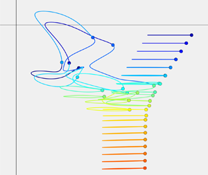
Figure 5. Eigenvalue orbits ((a,c,e,g) symmetric; (b,d,f,h) antisymmetric) at ${Re}=7500$ for four representative combinations of $Wo$ and $\tilde {Q}$ marked by yellow squares in figure 4(a) showing the variations possible in the parameter space. If present, the subharmonic orbits $\phi ^s_i$ and $\phi ^a_i$ are highlighted in colour. The black dots indicate the OS spectrum and the coloured dots the eigenvalue loci at the beginning of each period of $t$. Here (a,b) ${Wo}=15, \tilde {Q} = 0.1$; (c,d) 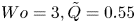${Wo}=3, \tilde {Q} = 0.55$; (e,f) 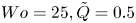${Wo}=25, \tilde {Q} = 0.5$; (g,h) 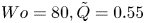${Wo}=80, \tilde {Q} = 0.55$.

We see that for a broad range of pulsation frequencies ($5 \leq {Wo} \leq 90$), subharmonic eigenvalue orbits are very common as the pulsation amplitude increases, starting as early as $\tilde {Q} = 0.07$ at ${Wo}=18$. Beyond this range, the subharmonic cycles appear at progressively higher amplitudes until, both for very low ($Wo=0.1$) and very high ($Wo=150$) pulsation frequencies, no subharmonic eigenvalue orbits are detected at all in the considered amplitude range. Based on the distributions in figure 4, it is to be expected that the range of pulsation frequencies that support subharmonic eigenvalue orbits will continue to widen as the pulsation amplitude is increased beyond $\tilde {Q} = 0.6$. Following the classification of the eigenvalues into the three branches A, P and S according to their location in the spectrum proposed by Mack (Reference Mack1976), we observe that the permutation cycles mostly start with eigenvalues located at the intersection of the three branches of the spectrum but quickly spread to include most eigenvalues of the A-branch. Only the outermost modes of the P-branch and very damped eigenvalues of the S-branch (marked in blue in the inset in figure 4a) maintain isolated orbits with the base flow frequency in the entire considered parameter range.

In figure 4(a), within the region where subharmonic eigenvalue orbits occur, we can further distinguish two parameter ranges with very different behaviour.

For intermediate pulsation frequencies (roughly $10 \leq {Wo} \leq 60$), only one or two permutation cycles form. The lengths of these cycles grow quickly as the pulsation amplitude increases and they eventually contain up to $m=15$ eigenvalues (${Wo}=8$ at $\tilde {Q}=0.6$). This is also the only region in which $\lambda _1$ and $\lambda _4$ eventually join the cycles and thus the dominant eigenvalues with temporarily positive growth rates are part of subharmonic orbits.

For pulsation frequencies below approximately $Wo=9$ or beyond $Wo=60$, instead of two large subharmonic orbits, we observe the emergence of up to seven distinct permutation cycles and the orbits of $\lambda _1$ and $\lambda _4$ merge, if at all, only for high pulsation amplitudes. Finally, for 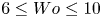$6 \leq {Wo} \leq 10$, there is also a sharp increase in the number of distinct subharmonic orbits as the pulsation amplitude increases beyond $\tilde {Q} = 0.55$, which coincides with a drastic reduction of the number of eigenvalues in $\varphi _1$ (figure 4b) indicating that the large orbit has disintegrated into a number of separate, shorter orbits.

In order to understand the effect of the pulsation frequency and amplitude on the formation of permutation cycles, it is instructive to consider the location of the orbits in the complex plane. In figure 5 each row shows all the eigenvalue orbits for one of the four numbered cases marked with yellow squares in figure 4(a) that highlight prominent features. In the following discussion we will denote by $\varphi ^s$ and $\varphi ^a$ the permutation cycles formed by symmetric and antisymmetric eigenvalues, respectively. The orbits in each figure are indexed by increasing stability.

Figure 5(a,b) shows a typical case at moderate pulsation frequency ($Wo=15$) where the amplitude $\tilde {Q}$ has crossed the critical threshold and the first subharmonic eigenvalue orbit (involving two antisymmetric modes) has appeared close to the intersection of the eigenvalue branches. We also observe the characteristic feature that the orbits corresponding to eigenvalues of the A-branch experience more pronounced excursions over a cycle, especially in terms of growth rate, than those of the P- and S-branches. The latter, instead, vary mainly along the imaginary axis, following the variation of the mass flow rate which can be seen from the fact that the eigenvalues have the largest (smallest) imaginary part at $t/T = 0$ ($t/T = 0.5$) where $Q(t)$ is maximal (minimal), the former marked by a filled dot along each orbit.

As the pulsation amplitude is increased, the subharmonic orbits expand and eventually encompass all eigenvalues of the A-branch, separated into two distinct permutation cycles based on their symmetry. Figure 5(e,f) show an example of this situation at $Wo=25$ and $\tilde {Q}=0.5$. Although the details of the orbits, especially for eigenvalues on the A-branch, vary considerably, all cases at intermediate pulsation frequencies are structurally similar to the case presented here featuring only two permutation cycles. Note that for this parameter combination, both $\varphi ^s_1$ and $\varphi ^a_1$ exhibit positive growth rates over part of the cycle.

For higher pulsation frequencies, the variation in the growth rate of the eigenvalues across the cycle reduces. Eventually, the orbits of $\lambda _1$ and $\lambda _4$, being relatively isolated in the spectrum, no longer merge into subharmonic orbits even at high pulsation amplitudes as shown in figure 5(g,h) for $Wo=80$ and $\tilde {Q}=0.55$. Nevertheless, the eigenvalues close to the intersection of the branches continue to form permutation cycles and exhibit complex orbits.

If we instead reduce the pulsation frequency, we see a smaller growth rate variation only for $\lambda _1$ and $\lambda _4$ while other eigenvalues from the A-branch and the intersection area exhibit strong variations in both real and imaginary parts across the cycle. Moreover, in this part of the parameter space, the leading eigenvalues do not form subharmonic orbits. It can also be noted that, unlike all cases at intermediate and high pulsation frequencies, the roughly oval orbits on the A- and P-branches at low Womersley numbers are tilted with the major axes pointing towards the origin of the complex plane.

The smooth orbits formed by the eigenvalue traces over a period are accompanied by the corresponding eigenvectors through the permutation cycle. The variation of the eigenvector of $\varphi ^s_1$ over a complete subharmonic cycle is shown in movie 1 of the supplementary material available at https://doi.org/10.1017/jfm.2022.515 for $Wo=25$, $\tilde {Q} = 0.2$ where $\varphi ^s_1$ has a period of $m=3$.

Within the parameter range considered in this work, the cases in which $\lambda _1$ eventually joins a subharmonic eigenvalue orbit are particularly interesting because the variation of the instantaneous operator spectrum has a large impact on the evolution of a linear perturbation. We will analyse the periodic orbits for three Womersley numbers in detail, namely $Wo=10$, 18 and 25, that span the range of pulsation frequencies of interest and exhibit very different behaviour as the pulsation amplitude is varied.

4.3. Time scale analysis

The qualitative differences in the spectra and hence the periodic eigenvalue orbits for different pulsation frequencies can be understood by comparing the time scale of the intrinsic instabilities of Poiseuille flow and the pulsation frequency.

Following the classical time scale analysis for parallel shear flow with considerable mean flow described in Davis (Reference Davis1976), the relevant time scale ratio between the principal viscous flow time scale and the pulsation time scale becomes

(4.3)\begin{equation} \mathcal{T} = \frac{2\beta^2}{{Re}} = \frac{{Wo}^2}{{Re}}, \end{equation}

where we note that, due to differing normalisations, the Womersley number $Wo$ and the frequency parameter $\beta$ (not to be confused with the spanwise wavenumber traditionally using the same symbol) are related as

(4.4)\begin{equation} \frac{\beta}{{Wo}} = \sqrt{2}. \end{equation}

An overview of the values of $\mathcal {T}$ for different values of the Womersley number including the range considered in this work, assuming a constant Reynolds number of $Re=7500$, are given in table 1.

Table 1. Overview of the range of time scale ratios of the viscous time scale and the pulsation time scale as a function of the Womersley number for $Re=7500$.

It is clear that for two different pulsation frequencies at the same Reynolds number, the time scale ratios $\mathcal {T}$ cannot be directly compared since the Womersley number affects both the pulsation time scale and the velocity profile. A more rigorous assessment of the separation of scales and the role of the Reynolds number can be made via a Wentzel–Kramers–Brillouin–Jeffreys (WKBJ) analysis in time (see Benney & Rosenblat Reference Benney and Rosenblat1964) but this analysis is outside of the scope of this work that focuses on the variation of the pulsation parameters ${Wo}$ and $\tilde {Q}$. For our purposes focusing on the emergence of subharmonic eigenvalue orbits it is sufficient to analyse the behaviour for extreme values of the pulsation frequency. We consider two cases in particular, namely $Wo\ll 1$ ($\mathcal {T}\ll 1$) and $Wo\gg 1$ such that $\mathcal {T} \gg 1$ for which the variation of the base flow profiles and corresponding eigenorbits over the pulsation cycle at $\tilde {Q} = 0.5$ are shown in figure 6.

Figure 6. Base flow profiles and corresponding eigenorbits for extreme values of the Womersley number at $\tilde {Q} = 0.5$. In this parameter range there are no subharmonic eigenvalue orbits. Here (a,b) ${Wo} = 0.1$; (c,d) ${Wo} = 300$.

We see from the definition that the time scale separation between viscous effects and the base flow pulsation scales with the square of the Womersley number and approaches zero for the lowest pulsation frequencies considered in this work, indicating that the flow in that parameter region is quasi-steady (QS), i.e. the pulsation period is so long that the flow can essentially adapt instantaneously to the changes in pressure gradient. The flow therefore behaves instantaneously like plane Poiseuille flow with a parabolic velocity profile, the pulsations only varying the effective Reynolds number. The corresponding periodic orbits have the base flow frequency and do not show any hysteresis over the cycle, i.e. there is no difference between the base flow acceleration and deceleration phases.

At the other extreme of the $Wo$-spectrum, for $\mathcal {T}\gg 1$, the pulsation cycles are so short compared with the viscous time scale that the flow does not have time to adapt at all and the velocity fluctuation induced by the varying pressure gradient and superimposed on the steady parabolic component increasingly resembles a top hat profile. The resulting base flow profile exhibits extremely thin oscillating boundary layers close to the walls but has an otherwise constant wall-normal variation that is translated along the streamwise direction during a pulsation cycle. In this regime, the orbits have the base flow frequency, exhibit no hysteresis and only oscillate along the imaginary axis synchronised with the pulsations. In fact, the second derivative of the base flow profile in the wall-normal direction, pivotal for its stability characteristics, is constant and equal to that of the steady Poiseuille flow everywhere with the exception of the oscillating boundary layer that is too thin to noticeably affect the instability waves since the inflection points are located too close to the wall (Kern et al. Reference Kern, Beneitez, Hanifi and Henningson2021).

The result that pulsations do not lead to an increased instability of the base flow profile for high pulsation frequencies is in line with the conclusions drawn in Davis (Reference Davis1976) with regard to the stability of highly inflectional Stokes layers that are dynamically similar for $\delta \ll h$ and are found to be unstable only for small pulsation frequencies. For pulsating Poiseuille flow, however, the results do not extend to very low frequencies ($Wo\ll 1$) since the comparison breaks down when the two Stokes layers merge at the centreline when $\delta \approx h$ and the base flow profile ceases to be inflectional.

From the time scale analysis we conclude that, while for intermediate values of $Wo$ the time scales associated with the base flow pulsation and viscous effects are similar and we thus see considerable variation of the stability characteristics with the Womersley number, the flow at very high (very low) pulsation frequencies only depends on the (effective) Reynolds number and we do not find any subharmonic eigenvalue orbits.

4.4. Pulsations and non-normal growth potential

In view of the considerable non-normality of the OS operator, the spectrum itself only paints only part of the picture. In order to fully examine the stability characteristics of the operator, it is crucial to consider the energy growth potential brought about by the superposition of non-orthogonal eigendirections with very different growth rates that can lead to large transient amplification of disturbances even in linearly stable flows (Reddy & Henningson Reference Reddy and Henningson1993; Trefethen et al. Reference Trefethen, Trefethen, Reddy and Driscoll1993). Of particular interest in the context of pulsating Poiseuille flow is the question how the non-normal growth potential, intrinsic to plane Poiseuille flow, is altered by the addition of a pulsatile component to the base flow. A common measure of this potential is the numerical abscissa of the operator, often denoted $\sigma _{max}$, which encodes the maximum instantaneous growth rate possible taking into account both modal and non-modal mechanisms (Trefethen & Embree Reference Trefethen and Embree2005; Schmid Reference Schmid2007). The numerical abscissa of a matrix $L$ is given by the largest eigenvalue of its Hermitian part, i.e. we have

(4.5)\begin{equation} \sigma_{max} = \lambda_{max}\left( \frac{1}{2} \left(L + L^H \right) \right), \end{equation}

where $(\,\cdot\,)^H$ denotes complex conjugation, and can also be computed as the maximum protrusion of the numerical range into the unstable half-plane (Trefethen Reference Trefethen1997).

In a recent study of the stability of pulsating Poiseuille flow, Kern et al. (Reference Kern, Beneitez, Hanifi and Henningson2021) have conjectured that, in spite of the considerable variation of the instantaneous eigenvalues over a cycle, the pulsations only have a negligible impact on the full non-normal growth potential. Due to the high computational cost of the method used in the study when aiming to capture the full non-normality of the operator, the impact of the pulsations on the non-modal growth potential was analysed only for the case ${Wo}=25$ and $\tilde {Q}=0.2$ where the numerical abscissa was found to fluctuate within 1 % of the corresponding steady value (${Re}=7500$, $\tilde {Q} = 0$) during the pulsation cycle.

Using the full operator from the local analysis, we can efficiently map the effect of pulsations on the numerical abscissa and test the conjecture over the full parameter range. In addition to the absolute value of $\sigma _{max}$ we will also consider $\Delta \sigma =\sigma _{max} - \sigma _{r}$, the fluctuation of the numerical abscissa with respect to the steady reference value $\sigma _{r}$, which is particularly useful for harmonic variations around the reference value. Based on the time scale analysis above, we can begin by defining the extremal values for the numerical range. For very large values of $Wo$, the numerical abscissa is equal to the steady value, i.e. $\Delta \sigma = 0$, since the spectrum is only translated along the imaginary axis. For very low pulsation frequencies, on the other hand, we are in the QS regime and the base flow profile $U_{QS}(t)$ is parabolic and synchronised with the fluctuating mass flow rate, such that

(4.6)\begin{equation} U_{QS}(t) = \frac{3}{2} \frac{Q(t)}{2h}(1-\xi^2), \end{equation}

where we have used the steady state relationship $Q = U_b 2h = \tfrac {2}{3} U_c 2h$ with $U_b$ the bulk velocity.

It is clear that the flow rate variations in the QS regime are equivalent to a variation of the Reynolds number in plane Poiseuille flow such that the numerical abscissa can be computed from the corresponding steady problem at each instant in the pulsation cycle. Therefore, the variation of the non-normal growth potential in the two extreme cases relies solely on the intrinsic non-normal growth mechanisms of steady Poiseuille flow. In the following, we will compare the corresponding profiles for the numerical abscissa with the data for intermediate pulsation frequencies.

The variation of the numerical abscissa for pulsating Poiseuille flow over the full range of pulsation frequencies and amplitudes considered in this work is shown in figure 7 compared with the QS limit (black dashed line). The first observation is that the relatively simple dependence of the numerical abscissa on the pulsation frequency and amplitude that is similar over the entire considered parameter range. This is in stark contrast with the complex behaviour of other spectral quantities such as the instantaneous eigenvalues (compare with the large variability of the eigenvalue orbits within the parameter range in figure 5) or the Floquet exponents (especially at low pulsation frequencies where the variation of the intercyclic stability is high non-monotonic, see Pier & Schmid (Reference Pier and Schmid2017) and Kern et al. (Reference Kern, Beneitez, Hanifi and Henningson2021)). Not only are the slopes of $\max _p |\Delta \sigma |$ similar, also the intracyclic variations of the numerical abscissa are highly regular for all but the highest pulsation frequencies which have negligible amplitude. The similarity of the intracyclic variation across the parameter range to the QS limit further supports the conclusion that the main mechanism generating it is the same. The comparison with the data from Kern et al. (Reference Kern, Beneitez, Hanifi and Henningson2021) shows very good agreement, in particular in terms of the intracyclic variation. The amplitude mismatch is minute considering that the corresponding amplitude $\max _p |\Delta \sigma |$ is around $1\,\%\:\sigma _r$ and shows that the computation indeed captured nearly the fully non-normal growth potential.

Figure 7. Variation of the numerical abscissa $\sigma _{max}$ of the OS operator for pulsating Poiseuille flow at ${Re}=7500$ and $(\alpha,\beta )=(1,0)$ as a function of time and the pulsation frequency and amplitude. (a) Variation of the numerical abscissa over the pulsation cycle for different pulsation frequencies for $\tilde {Q}=0.2$ compared with the variation in the QS limit (dashed line). (b) Same data as in (a) but presenting $\Delta \sigma$ normalised by the maximum deviation from the steady value over the period to highlight the intracyclic variation at different frequencies. The dots correspond to the data from Kern et al. (Reference Kern, Beneitez, Hanifi and Henningson2021) using $r= 100$ modes (cf. figure 10 in Kern et al. (Reference Kern, Beneitez, Hanifi and Henningson2021)) for the same case.

The orderly variation of the numerical abscissa across the considered parameter range is all the more surprising given the fact that is uncorrelated with the leading eigenvalues of the Jacobian, both in terms of intracyclic variation and in amplitude. It is especially striking that we do not see any trace of the EPs that are so abundant in the spectrum and are characterised by eigenvector coalescence and thus lead to highly non-orthogonal eigenvectors in their vicinity. There are two explanations for this fact. Firstly, for non-normal growth to occur involving two non-orthogonal eigendirections, it is not sufficient for them to be nearly colinear but they also require very different growth rates. Since the coalescing eigenvectors, instead, have more similar growth rates the closer they come to the EP, they cannot, by themselves, generate considerable non-normal growth. Secondly, the non-modal growth mechanisms intrinsic to plane Poiseuille flow that lead to the maximum transient growth rely on very damped modes. In particular, $r=100$ real modes (which corresponds to 50 complex modes) are necessary to map the full potential which includes modes from the S-branch that are considerably less affected by the pulsation than the modes from the A-branch that predominantly form the permutations cycles. These modes in fact exhibit a harmonic variation over the pulsation cycle and exhibit considerable growth rate variations only for low values of the Womersley numbers where the flow is close to the QS regime (compare the most damped modes in figure 5) which is in line with the behaviour of the numerical abscissa.

Based on these analyses, the conjecture that the addition of a pulsatile component does not considerably alter the perturbations having the maximum non-normal growth potential in two-dimensional Poiseuille flow can be confirmed. The intracyclic variations of the numerical abscissa over the full range of Womersley numbers, not only in the limiting cases, are caused by the mechanisms intrinsic to plane Poiseuille flow that dependent on the effective Reynolds number instead of the details of the oscillating base flow profile. The mechanisms that are dependent on the modes that experience modulation due to the pulsations lead to smaller non-normal growth and therefore have no repercussion on the numerical abscissa.

This conclusion is in line with results from the recent work by Pier & Schmid (Reference Pier and Schmid2021) where the authors computed the optimal transient growth curves for two- and three-dimensional disturbances in pulsating Poiseuille flow that showed the universality of the Orr mechanism and the lift-up effect in optimal non-modal growth known from steady Poiseuille flow also in the pulsating case. The study found that for pulsating Poiseuille flow the largest transient growth is achieved either via the lift-up effect like in the steady case for low pulsation amplitudes (largely independent of the frequency) or, as the pulsation amplitude increases, via the Orr mechanism. The two-dimensional mechanism takes over as the driver for maximum energy growth since the perturbation first grows via the Orr mechanism just before the phase of linear instability where it switches gears and takes advantage of the modal growth of the unstable eigenvalue that increases exponentially with the pulsation amplitude. The analysis of the numerical abscissa shows that non-normal growth in pulsating Poiseuille flow is fundamentally similar to the steady counterpart not only for the optimal initial condition but also for the instantaneously most amplified structure.

5.1. Effect of EPs on the linear IVP

The first question of interest regarding the solution of the IVP in the context of EPs is which effect the eigenvalue degeneracies have directly on the linear solution and, in particular, what happens to the solution close to a degeneracy. In our study, we have not been able to detect any abrupt or notable changes in the instantaneous linear solutions as the pulsation amplitude is increased past a bifurcation point where an EP occurs during the period. As a typical example, we consider the same case as for the identification of the EPs (figure 3, i.e. ${Wo}=25$) and compare the linear solutions computed for three different pulsation amplitudes around the critical value at which the EP forms. It turns out that the linear growth rates, shown in figure 8, behave nearly identically both before, after and very close to the bifurcation point. This is not particularly surprising considering the ubiquity of EPs we have documented together with the facts that in steady flows energy growth varies smoothly (channel flow (Reddy & Henningson Reference Reddy and Henningson1993)) and spectral degeneracies have been studied previously without uncovering traces of dramatic growth variations for nearly degenerate operators (Gustavsson & Hultgren Reference Gustavsson and Hultgren1980; Koch Reference Koch1986; Shanthini Reference Shanthini1989). Note that the operator is never exactly degenerate numerically.

Figure 8. Instantaneous perturbation growth rates for three configurations from figure 3 close to $\tilde {Q}_{crit}$ over one period after the transients have passed. The grey lines indicate the instantaneous symmetric spectrum at $\tilde {Q}_{crit}$ and the eigenvalue orbits merging at the EP (marked with a red cross) are highlighted in black (solid and dashed). The colour coding for the IVP solutions is the same as for the corresponding spectra in figure 3.

5.2. Branch transition on subharmonic eigenvalue orbits

Although the EPs themselves do not seem to leave any traces in the evolution of a linear perturbation, they have a pronounced effect via the formation of subharmonic eigenvalue orbits.

The evolution of the linear perturbation, at each instant in time, is dictated by the instantaneous spectrum of the OS operator. Since the operator changes continuously, the perturbation never fully aligns with the dominant eigendirection for long times as we would expect in the steady case. Nevertheless, the perturbation, so long as it has a projection on an instantaneous eigendirection, will grow in that direction and preferentially towards the dominant eigenstate. Two major factors governing this alignment are therefore the rate at which the eigenstates change compared with their instantaneous growth rates and the difference between the growth rates of the dominant and subdominant eigenstates with a considerable projection on the instantaneous perturbation.

This imperfect alignment with the dominant eigendirection can be seen in figure 9 comparing the instantaneous growth rates of the linear solution with the corresponding symmetric spectrum (only the symmetric spectrum is shown since the linear perturbation is always symmetric in the periodic regime and therefore the asymmetric modes are irrelevant) for a wide range of pulsation frequencies and amplitudes. The alignment is best when the eigenstates only change slowly (typically, a slow variation of the growth rate is linked to a slow variation of the eigenvector for shown here) and the dominant eigenvalue grows much faster than the subdominant, such as during the amplification phase at low pulsation frequencies (column 3). On the other hand, the alignment is less pronounced at higher pulsation frequencies where the operator changes quickly (column 1) as well as during the damping phases where dominant and subdominant eigenvalues exhibit similar growth rates. In these regions we also see considerable growth rate overshoots/undershoots and wiggles. These wiggles, although they already appear earlier, become particularly pronounced once the dominant eigenvalue forms a subharmonic orbit (see figure 9d,e,i) and are linked to the transition of the linear perturbation from the decaying branch to the amplified branch of the eigenvalue orbit. The branch transition is necessary because, as we know from Floquet theory, the linear perturbation eventually settles into a periodic motion at the same frequency as the base flow once the initial transients have passed. As the branch transition happens during a part of the cycle where the spectrum is heavily damped and the perturbation is influenced by several non-orthogonal decaying eigendirections at the same time, it is likely that the wiggles are due to non-normal growth bursts. For very large pulsation amplitudes, the wiggles are suppressed and the branch transition is increasingly abrupt (see figure 9j–k).

Figure 9. Evolution of the perturbation growth rate (thick coloured line) after the transients have passed compared with the real part of the instantaneous symmetric spectrum (grey lines) over three consecutive periods for different pulsation frequencies and amplitudes at $Re=7500$. The dominant eigenvalue orbit is highlighted and, if it is subharmonic, the same orbit in adjacent periods are marked in black as dotted and dashed lines. In these cases, a movie comparing flow fields of the linear perturbation with the instantaneous eigenvectors of adjacent branches of the dominant orbit are available in the supplementary material (linked in the description). Here (a–c) $\tilde {Q}=0.08$; (d–f) $\tilde {Q}=0.18$; (g–i) $\tilde {Q}=0.28$ (j–l) $\tilde {Q}=0.50$. Here (a,d,g,j) ${Wo}=25$ (blue); (b,e,h,k) ${Wo}=18$ (red); (c,f,i,l) ${Wo}=10$ (yellow).

We know that the non-normal growth mechanisms from plane Poiseuille flow and hence their time scales are essentially unchanged when pulsations are added both instantaneously (see § 4.4) and when considering optimal disturbances (Pier & Schmid Reference Pier and Schmid2021). It is therefore useful to compare the time scale of the growth bursts we observe in the periodic regime with that of the Orr mechanism, central to optimal transient growth of two-dimensional disturbances. Considering the IVP for plane Poiseuille flow, the optimal initial condition for maximum transient growth at $Re=7500$ with $\alpha =1$ (close to the transiently most amplified streamwise wavenumber) reaches the maximum energy at $t_{Orr}=27 t_U$ with the mean flow advection time scale $t_U = h^2/Q^{(0)}$. Figure 10(a) shows the energy growth envelope for plane Poiseuille flow for this case with $t_{Orr}$ marked by the red line. In figure 10(b), we compare the growth rate wiggles for different pulsation frequencies to this transient growth time scale. We see that the growth bursts all happen on the same time scale that compares very well with the time scale of the Orr mechanism.

Figure 10. Definition of the non-normal growth time scale $t_{Orr}$. (a) Growth envelope for maximum transient growth for plane Poiseuille flow at at $Re=7500$ and $\alpha = 1$. The energy maximum at $t_{Orr}$ is indicated with a red dot. (b) Superposition of the wiggles in the growth rates of for three configurations with time scaled by $t_{Orr}$. Since the wiggles occur at very different times in each case, the curves are shifted by $t_0$ (different in each case) to facilitate direct comparison.

In a second step, we take a closer look at one particular case, ${Wo}=18$, $\tilde {Q} = 0.16$ (figure 9e), where the wiggles are particularly pronounced. In figure 11, the variation of the dominant subharmonic eigenvalue orbit during the damping phase is shown together with snapshots of the streamwise velocity component of the associated eigenvectors as well as the linear perturbation for the full the branch transition. This parameter combination highlights the typical features of the branch transition while the dominant permutation cycle only contains two eigenvalues which makes the presentation more clear. The essential features of the transition process are the same in all cases considered in this work.

Figure 11. Variation of the streamwise velocity field and the growth rate of the linear perturbation centred on the branch transition compared with the dominant eigenstate orbit at $Re=7500$, $Wo=18$, $\tilde {Q} = 0.16$ (same case as in figure 9e). (a–c) Variation of the real and imaginary parts ((a) and (b), respectively) of the instantaneous eigenvalues along the subharmonic orbit $\varphi ^s_1$ (black lines) compared with the growth rate of the linear perturbation (thick blue line). The two branches of $\varphi ^s_1$ are distinguished by the dashed and full linestyles and the angle $\theta$ (in radians) between the corresponding eigenvectors is shown in panel (c). (d–f) Instantaneous streamwise velocity fields of the linear perturbation and eigenvectors of $\varphi ^s_1$, each column corresponding to a time instant marked by a vertical line in (a–c). Panel (d) corresponds to the linear perturbation ($u_{lin}$) whereas the panel (e,f) shows the instantaneous eigenvectors of the branches $u_0$ (full black line) and $u_{1}$ (dashed line) of $\varphi ^s_1$. The $y$-direction is the wall-normal direction and the $x$-direction is the streamwise direction. A movie of the variation in time is available in the supplementary material (movie 2).

Let us first analyse the variation of the instantaneous eigenstates along the two branches $u_0$ and $u_1$ of the dominant subharmonic orbit before comparing it with the linear perturbation.

At the beginning of the considered section, which corresponds to the end of the amplification phase ($t_1$), we observe that the two branches of the orbit are very different, both in terms of growth rate and in spatial structure. With the beginning of the damping phase ($t/T=0.80$), the eigenstates (eigenvalues and eigenvectors) quickly converge and are very similar at $t_2$. This point is very close to the EP at which the subharmonic orbit formed and of which the minimum of the angle $\theta$ is the vestige. Their paths subsequently diverge again. During the damping phase, the growth rate of $u_0$ drops as the vortices of the eigenvector are sheared by the base flow an move away from the wall ($t_2$ and $t_3$). The imaginary part of the eigenvalue reflects the increased base flow velocity at the location of the dominant vortex row by steadily increasing up until $t_4/t_5$ where the heavily sheared vortices of the eigenvector $u_0$ stop moving towards the centreline. Simultaneously, the growth rate of $u_1$, which was very damped at $t=t_1$, increases continuously, passing $u_0$ at $t_3$ and changing sign at $t_7$ thus initiating the amplification phase. In contrast to $u_0$, for which the vortices move to the centreline while experiencing intense shear, the eigenvector of $u_1$ is pushed towards the wall which is echoed by a decrease of the imaginary part (phase speed) of the corresponding eigenvalue. These two opposite effects lead to the large difference in phase speeds between $u_0$ and $u_1$ that we observe throughout the damping phase.

Consider now the evolution of the linear perturbation $u_{lin}$ in the limit cycle over the same period and how it relates to the instantaneous eigenvectors described above.

Initially, the perturbation is aligned with the direction $u_0$ exhibiting the structure of modulated Tollmien–Schlichting waves typical of the amplification phase of pulsating Poiseuille flow ($t_1$). The subsequent variation of the eigenvectors heralding the damping phase is too rapid to be followed instantaneously by the linear perturbation and we observe that the growth rate only slowly decreases and changes sign at $t_2$ with considerable delay compared with $u_0$. The vortices in the linear perturbation are soon also sheared with the mean flow which is accompanied by strong damping ($t_3$). In the subsequent phase, all eigenvalues are damped and the linear perturbation has a non-zero projection on both $u_0$ and $u_1$ that are far from orthogonal during the branch transition process and can thus lead to non-normal growth. In fact, we see the footprint of both eigenvectors in the perturbation field which exhibits a row of vortices close to the wall ($u_1$) as well as sheared vortices closer to the centreline ($u_0$). The wiggles in the growth rate occur due to the rapid changes in the structure of $u_{lin}$. The difference in phase speed of the eigenvectors related to the difference in magnitude of the imaginary parts of $u_0$ and $u_1$ leads to a large relative velocity difference in the streamwise translation of the vortex rows in the linear perturbation. It is the interaction of these vortices that creates the strong variations in the growth rate we see in the perturbation in figure 11(a–c). During each growth burst, the vortex rows begin paired with alternating orientations. As the faster moving inner vortex row moves ahead of the outer row, the vortices of the same orientation merge to form large structures leaning against the mean shear extracting energy from the base flow in a manner analogous to the Orr mechanism generating large growth ($t_5$ and $t_7$). Subsequently, the vortices experience a strong decay when they are sheared with the mean shear ($t_4$ and $t_5$). During the branch transition process, the focus of the perturbation steadily moves from the vortices close to the centreline to the vortex row close to the wall together with the increasing growth rate gap in the corresponding instantaneous eigenvalues. As soon as $u_1$ starts to be amplified $t_7$, the wiggles quickly disappear as $u_{lin}$ aligns with the newly amplified eigenvector ($t_8$ and $t_9$).

In order to allow the reader to fully appreciate the similarities and differences across the considered parameter range, we have created a movie that is available in the supplementary material comparing the evolution of the linear perturbation with the instantaneous eigenstates in terms of both the growth rate and the spatial structure for the case shown in figure 11 where the leading eigenvalue has joined a permutation cycle and thus branch transition occurs.

Based on this analysis, the wiggles in the instantaneous growth rate observed during the branch transition process are indeed caused by repeated non-normal instantaneous transient growth bursts that are very similar to the Orr mechanism. All the cases considered in this work exhibiting a branch transition follow the same path.

5.3. Instantaneous non-normal growth and Floquet eigenfunctions in periodic flows

Time-periodic flows such as pulsating Poiseuille flow are special cases of time-dependent flows for which the time-asymptotic behaviour of a linear perturbation can be represented by the Floquet eigenfunctions (Davis Reference Davis1976). The variations of the growth rate during the pulsation cycle that we have identified as non-normal growth bursts are included and contribute to the Floquet multipliers that quantify the cycle-to-cycle growth of the eigenfunctions. This fact does not preclude an analysis of the growth bursts as instantaneous phenomena linked to the local eigenvalue spectra in time. The leading Floquet eigenfunction is, in fact, identical to the solution of the linear IVP after the initial transients have passed, as computed in this study using a time stepper approach; whether the instantaneous transient growth bursts are understood as manifestations of the global dynamics (Floquet) or an instantaneous effect of the local (in time) dynamics differs only in the interpretation.

The local interpretation of transient growth that we propose here is useful for two reasons. On the one hand the direct comparison with the local spectra elucidates the instantaneous growth mechanism allowing for the distinction of phases dominated by modal or non-modal growth within the pulsation cycle. This analysis is not directly possible within the Floquet framework since it involves a Fourier transform and is therefore delocalised in time. On the other hand, the interpretation of instantaneous growth in terms of local spectra can be extended to non-periodic time-dependent cases where Floquet theory cannot be applied, given a sufficient time scale separation between viscous/inertial time scales of the flow and the imposed time-dependence. In the case of arbitrary time-dependence of the flow without scale separation the local approach is questionable. A possible way forward in this scenario is the analysis of the left and right singular vectors of the fundamental solution matrix (see, e.g. Schmid Reference Schmid2007).

Due to the special care that needs to be taken when applying the nomenclature related to transient and non-normal growth, typically discussed in steady scenarios, in a time-dependent setting, we propose a disambiguation in the Appendix B.

5.4. Variation of the spanwise wavenumber and the Reynolds number

In this study, we have restricted the detailed analysis to the two-dimensional configuration with a streamwise wavenumber $\alpha =1$ and a Reynolds number of 7500, which is slightly supercritical in the corresponding steady case. In order to assess the general validity of our approach and analysis also beyond the scope of the chosen parameter range, it is important to consider the effect of a variation of the Reynolds number and the streamwise wavenumber $\alpha$.

The Reynolds number governs the viscous time scale (i.e. the time scale on which viscosity is dominant) of the system and measures the ratio of inertial to viscous forces in the flow. In general, an increase (decrease) of the Reynolds number leads to a decrease (increase) of the base flow stability and sparsity of the spectrum (i.e. the distance between neighbouring eigenvalues) but the non-normality remains. We know that for intermediate values of the Womersley number, the pulsations lead to increasingly large excursions of the eigenvalues, both in term of growth rate and phase speed, and the formation of EPs as the pulsation amplitude grows. In terms of the spectrum and the emergence of subharmonic orbits, an increase of the Reynolds number leads to larger excursions of the eigenvalues over a pulsation cycle and, in general, earlier formation of subharmonic orbits, and vice versa. Since the non-normal growth potential decreases with the Reynolds number, the transient growth bursts during branch transitions follow suit. Figure 12(a) shows how the Reynolds number affects the appearance of subharmonic eigenvalue orbits (only the symmetric case is shown).

Figure 12. (a) Same as figure 4(b) but showing the appearance of the first subharmonic orbit involving the dominant symmetric eigenvalue for different Reynolds numbers. The red line is the same as the limit of the coloured area in figure 4(b). (b) Growth rate of the most amplified wavenumber for different pulsation amplitudes at ${Re}=7500$ and for ${Wo} = 10, 18, 25$, (dashed, dotted and full lines, respectively).

The streamwise wavenumber $\alpha = 1$ for this study was chosen close to the most unstable spanwise invariant configuration for steady Poiseuille flow. When pulsations are added, we observe not only a large variation of the instantaneous spectrum but also a shift in the most amplified streamwise wavenumber over the course of the pulsation cycle. Figure 12(b) shows, for each wavenumber, the maximum growth rate of the dominant eigenvalue of the local spectra at any time during the pulsation cycle. As expected, the maximum growth rates increase for all wavenumbers with the pulsation amplitude, irrespective of the pulsation frequency. At the same time the overall most amplified wavenumber shifts to slightly higher values.

In spite of these differences, the solutions to the IVP in the periodic regime do not change qualitatively. Since the time scale ratio $\mathcal {T}$ is inversely proportional to the Reynolds number, a decrease of the Reynolds number leads to an increase of the time scale ratio (and vice versa) meaning that the viscous time scale becomes slower relative to the pulsation time scale and the linear solution lags behind the instantaneous spectra even for low values of the Womersley number.

5.5. Outlook on three-dimensional perturbations

Given the well known fact that three-dimensional perturbations often generate far greater transient growth than their two-dimensional counterparts and, moreover, that the recent study of Pier & Schmid (Reference Pier and Schmid2021) has shown that the mechanism for optimal initial transient growth can be either two-dimensional or three-dimensional depending on the parameter configuration, it is a natural next step to ask whether the bursts during the transition process will exhibit a similar behaviour.

The mathematical properties that give rise to EPs and thereby lead to the formation of subharmonic eigenvalue orbits, i.e. the non-normality of the linear operator, do not depend on the spatial structure of the perturbations considered. If anything, the additional parameter makes the appearance of EPs more likely. Therefore, the results regarding the appearance and distribution of the eigenvalue permutation cycles in the considered parameter space vary only quantitatively as the spanwise wavenumber is varied and are not shown here.

In this work, only two-dimensional perturbations were considered in detail to keep the parameter space manageable. Since the qualitative behaviour of EPs and subharmonic eigenvalue orbits is the same as for the two-dimensional case and we have data regarding optimal energy growth (Pier & Schmid Reference Pier and Schmid2021) for the three-dimensional case, we can speculate about the effect of allowing three-dimensional perturbations on the solution of the linear IVP.

The existence of subharmonic eigenvalues orbits involving the leading eigenvalue also when $\beta \neq 0$ implies the necessity of branch transitions in the periodic regime in these cases likely driven by non-normal growth bursts. Considering that, as Pier & Schmid (Reference Pier and Schmid2021) note, ‘streamwise-invariant ($\alpha =0$) perturbations appear to be almost unaffected by the time-dependent component of the base flow and to display a dynamics predominantly dictated by the time-averaged base flow’, it is unlikely that a considerable streamwise-invariant component of the perturbation is part of the intrinsic linear dynamics of pulsating Poiseuille flow which fully determine the solution in the time-asymptotic periodic regime. Hence the authors expect the behaviour of the linear IVP allowing for three-dimensional perturbations to be qualitatively similar in the periodic regime to the results shown here, in particular regarding the nature of the non-normal growth bursts via a predominantly two-dimensional mechanism.