


1. Introduction
Crossflow instability (CFI) is one of the dominant instability mechanisms in a subsonic three-dimensional boundary layer over swept wings. Such CFI arises due to the inflection point in the velocity profile of the crossflow (CF) component and can have a stationary or travelling nature, depending on the receptivity process, the level of free-stream turbulence and surface roughness. In low-free-stream-turbulence environments, such as free flight conditions of commercial airliners, the stationary CFI becomes dominant, while the travelling CFI becomes dominant when the level of free-stream turbulence is high (Deyhle & Bippes Reference Deyhle and Bippes1996). The stationary CFI manifests itself as co-rotating vortices that develop in a direction closely aligned with the inviscid external streamline (Saric, Reed & White Reference Saric, Reed and White2003).
The CFI-dominated laminar–turbulent transition on a smooth swept wing (i.e. without surface irregularities or enhanced roughness) commonly occurs due to the development of type I, type II or type III secondary instabilities. Type I secondary instability, also known as the
 $z$
mode, originates in the outer part of the CF vortex (CFV) upwelling region, where the spanwise shear reaches its local minimum (Malik et al. Reference Malik, Li and Chang1996, Reference Malik, Li, Choudhari and Chang1999; Wassermann & Kloker Reference Wassermann and Kloker2002). Type II secondary instability (
$z$
mode, originates in the outer part of the CF vortex (CFV) upwelling region, where the spanwise shear reaches its local minimum (Malik et al. Reference Malik, Li and Chang1996, Reference Malik, Li, Choudhari and Chang1999; Wassermann & Kloker Reference Wassermann and Kloker2002). Type II secondary instability (
 $y$
mode) originates at the top of the CFV and away from the wall, where wall-normal shear has its local maximum (Malik et al. Reference Malik, Li and Chang1996, Reference Malik, Li, Choudhari and Chang1999; Wassermann & Kloker Reference Wassermann and Kloker2002). Lastly, the so-called type III mode describes the interaction between stationary and travelling primary CFI modes. It is located in the inner part of the upwelling region of the CFV, and coincides with the local maximum of spanwise shear (Bonfigli & Kloker Reference Bonfigli and Kloker2007).
$y$
mode) originates at the top of the CFV and away from the wall, where wall-normal shear has its local maximum (Malik et al. Reference Malik, Li and Chang1996, Reference Malik, Li, Choudhari and Chang1999; Wassermann & Kloker Reference Wassermann and Kloker2002). Lastly, the so-called type III mode describes the interaction between stationary and travelling primary CFI modes. It is located in the inner part of the upwelling region of the CFV, and coincides with the local maximum of spanwise shear (Bonfigli & Kloker Reference Bonfigli and Kloker2007).
Reducing the growth of stationary CFVs, and consequently reducing the growth of secondary instabilities to extend the laminar region through laminar flow control (LFC) techniques, has been the topic of research for several decades. Two broad and important categories of LFC strategies are upstream flow deformation (UFD) (Wassermann & Kloker Reference Wassermann and Kloker2002) and base flow modification. While UFD techniques directly target the critical instability mode, base flow modification alters the velocity profile where instabilities develop, aiming to reduce the strength of the inflectional CF velocity component in the base flow.
One of the successful UFD strategies is the use of micron-sized discrete roughness elements (DREs) positioned at a spacing smaller than the wavelength of the naturally most amplified CF mode (Reibert et al. Reference Reibert, Saric, Carrillo and Chapman1996; Saric et al. Reference Saric, Carrillo and Reibert1998b ). The effectiveness of this approach has been demonstrated in both wind-tunnel experiments (Saric et al. Reference Saric, Carrillo and Reibert1998a ; Kachanov, Borodulin & Ivanov Reference Kachanov, Borodulin and Ivanov2015) and numerical simulations (Wassermann & Kloker Reference Wassermann and Kloker2002; Rhodes et al. Reference Rhodes, Reed, Saric, Carpenter and Neale2010; Rizzetta et al. Reference Rizzetta, Visbal, Reed and Saric2010; Hosseini et al. Reference Hosseini, Tempelmann, Hanifi and Henningson2013). However, this method is highly sensitive to background roughness and to the baseline transition location (Lovig, Downs & White Reference Lovig, Downs and White2014; Saric et al. Reference Saric, West, Tufts and Reed2019). Another UFD-based approach employs spanwise-modulated plasma actuators to influence the most amplified CF mode (Dörr & Kloker Reference Dörr and Kloker2017; Serpieri, Venkata & Kotsonis Reference Serpieri, Venkata and Kotsonis2017; Shahriari, Kollert & Hanifi Reference Shahriari, Kollert and Hanifi2018). Examples of base flow modification techniques include wall suction/blowing (Messing & Kloker Reference Messing and Kloker2010) and the use of plasma actuators to induce a two-dimensional volume forcing against the local CF velocity component (Dörr & Kloker Reference Dörr and Kloker2015; Yadala et al. Reference Yadala, Hehner, Serpieri, Benard, Dörr, Kloker and Kotsonis2018), both of which have been shown to delay transition. A review of LFC techniques for CFI-dominated boundary layers can be found in Messing & Kloker (Reference Messing and Kloker2010) and Saric, Carpenter & Reed (Reference Saric, Carpenter and Reed2011).
While LFC techniques aim to delay transition, real-world surface irregularities can either hinder or enhance these efforts, depending on their interaction with CFVs. Understanding the interactions between CFVs and unavoidable surface features on real wings, such as gaps, steps, waviness and smooth humps, is therefore crucial for practical LFC applications. Such understanding helps to identify the surface features that degrade the effectiveness of LFC by advancing the onset of transition (compared with an ideal smooth design), and those that potentially delay the transition by suppressing instability growth, thereby suggesting novel LFC techniques. The following provides a brief overview of previous studies examining the interaction between CFVs and surface irregularities, and how this interaction influences instability growth and the transition to turbulence.
The interactions between CFVs and forward-facing (FFS) and backward-facing (BFS) steps have been studied extensively. Many studies have shown that both FFS and BFS enhance the growth of CFVs downstream of the step location and shift the transition location upstream compared with a scenario in which no geometrical feature is present on the surface (e.g. Tufts et al. Reference Tufts, Reed, Crawford, Duncan and Saric2017; Eppink Reference Eppink2020, Reference Eppink2022; Rius-Vidales & Kotsonis Reference Rius-Vidales and Kotsonis2020, Reference Rius-Vidales and Kotsonis2021, Reference Rius-Vidales and Kotsonis2022). Moreover, Eppink (Reference Eppink2020) and Rius-Vidales & Kotsonis (Reference Rius-Vidales and Kotsonis2022) showed that, if the height of the FFS is larger than a given threshold, the step can even trip the boundary layer, and transition occurs at the step location. This critical threshold, however, depends on the amplitude of the incoming CFVs (Eppink Reference Eppink2020; Rius-Vidales & Kotsonis Reference Rius-Vidales and Kotsonis2020). For such conditions, Rius-Vidales & Kotsonis (Reference Rius-Vidales and Kotsonis2022) showed that the laminar–turbulent transition does not occur due to the onset of classic type I/II/III secondary CFI modes. Instead, it is driven by a distinct unsteady mechanism caused by locally enhanced spanwise-modulated shears and the recirculation region in the immediate downstream vicinity of the FFS. This finding emphasises the need for a more detailed analysis of CFV breakdown in the presence of surface irregularities. Despite the general consensus that FFS have a detrimental effect on the breakdown of CFVs, Rius-Vidales & Kotsonis (Reference Rius-Vidales and Kotsonis2021) showed that swept-wing transition delay can be achieved using a FFS of sufficiently small height. Furthermore, steady-state direct numerical simulations (DNS) by Casacuberta et al. (Reference Casacuberta, Hickel, Westerbeek and Kotsonis2022) attributed the stabilising effect of FFS on the CFI to the way energy is transferred between the base flow and the primary CF perturbations. Recently, Casacuberta, Hickel & Kotsonis (Reference Casacuberta, Hickel and Kotsonis2024) showed that a reverse lift-up effect might be one of the dominant mechanisms behind the observed primary CFI stabilisation effect.
Beyond nominal geometries such as FFS and BFS, the interactions between CFVs and more general smooth surface protrusions have not been studied extensively. Cooke et al. (Reference Cooke, Mughal, Sherwin, Ashworth and Rolston2019) studied the effect of localised bumps (i.e. combination of an FFS with BFS) on both stationary and travelling CFIs. They used the linearised harmonic Navier–Stokes method for their study and showed that the localised bumps, in general, enhance the growth of CFIs. However, they showed that for small height of the bumps, travelling CFI can become more stable. Thomas et al. (Reference Thomas, Mughal, Gipon, Ashworth and Martinez-Cava2016) studied the interaction between surface waviness and CFIs, using linear parabolised stability equations and linearised Navier–Stokes equations. They showed that whether surface waviness stabilises or destabilises the CFI depends on the spatial phase of the waviness. Westerbeek & Kotsonis (Reference Westerbeek and Kotsonis2022) studied the effect of surface waviness on the growth of primary CFI using nonlinear parabolised stability equations (NPSEs). For the particular shape of waviness they considered, the results showed destabilisation of primary CFI.
Westerbeek et al. (Reference Westerbeek, Sumariva, Alberto, Michelis, Hein and Kotsonis2023) studied the interaction between a smooth surface hump (with a concave–convex–concave shape) and stationary CFI by solving linear and nonlinear harmonic Navier–Stokes equations. For specific conditions, their results showed a stabilisation of the primary CFI mode downstream of the surface hump with respect to the clean flat plate case. A local destabilisation of higher harmonics of the primary CFI mode was also observed downstream of the hump, relative to the clean configuration.
More recently, Rius-Vidales et al. (Reference Rius-Vidales, Morais, Westerbeek, Casacuberta, Soyler and Kotsonis2025) have experimentally investigated the interactions between a smooth surface hump and stationary CFVs at low and high initial amplitudes, preconditioned by discrete roughness elements close to the leading edge. In the high-amplitude case, the amplitude of the stationary CF perturbation measured at 13 % of the chord was approximately 2.6 times larger than in the low-amplitude case. In the high-amplitude case of their experiments, abrupt transition to turbulence slightly downstream of the hump was observed. However, in the low-amplitude case of the experiments, stabilisation of stationary CF perturbations occurred downstream of the hump. This stabilisation resulted in a significant transition delay of about
 $ 14 \,\%$
of the chord compared with the reference (i.e. without hump) case. Detailed boundary-layer flow measurements showed a change in the orientation of CFVs downstream of the hump, which they related to a possible weakening or reversal of CF velocity component due to local pressure gradient changes by the hump geometry. Moreover, they observed that a notable change in the orientation of CF perturbations contributed to the stabilisation of the primary stationary CFI mode. This led to the eventual delay of transition to turbulence through the weakening of spanwise shears which affect the development of type I secondary CFI modes.
$ 14 \,\%$
of the chord compared with the reference (i.e. without hump) case. Detailed boundary-layer flow measurements showed a change in the orientation of CFVs downstream of the hump, which they related to a possible weakening or reversal of CF velocity component due to local pressure gradient changes by the hump geometry. Moreover, they observed that a notable change in the orientation of CF perturbations contributed to the stabilisation of the primary stationary CFI mode. This led to the eventual delay of transition to turbulence through the weakening of spanwise shears which affect the development of type I secondary CFI modes.
Westerbeek, Casacuberta & Kotsonis (Reference Westerbeek, Casacuberta and Kotsonis2026) studied the linear and nonlinear interactions between stationary CFVs and a smooth hump for various amplitudes of CF perturbations, using the steady harmonic Navier–Stokes method. They observed stabilisation of CFI when the amplitude of incoming CF perturbation is low. In agreement with Rius-Vidales et al. (Reference Rius-Vidales, Morais, Westerbeek, Casacuberta, Soyler and Kotsonis2025), they showed that the tilting of CF perturbations downstream of the hump is followed by their stabilisation.
The experiments of Rius-Vidales et al. (Reference Rius-Vidales, Morais, Westerbeek, Casacuberta, Soyler and Kotsonis2025) highlight the potential of using smooth surface humps as a practical passive control device to delay laminar–turbulent transition, which merits detailed analysis and understanding of both steady and unsteady mechanisms leading to transition delay or advancement. Currently available numerical works exploring these interactions have been limited to analysis of the flow from a steady-state point of view, which shed light on some of the steady mechanisms underlying the stabilising effect of the hump. However, development of unsteady secondary CFI modes determines the eventual delay/advancement of the transition location. Consequently, through DNS, this work aims to present an in-depth analysis of both the steady and unsteady mechanisms responsible for delaying or advancing the laminar–turbulent transition when the surface of a swept wing features a smooth hump at flow conditions comparable to those of the experiments of Rius-Vidales et al. (Reference Rius-Vidales, Morais, Westerbeek, Casacuberta, Soyler and Kotsonis2025). Regarding the low-amplitude perturbation case, the key question is why and how the interaction between the hump and the CFVs leads to the stabilisation of the stationary primary CFI. The impact of this stabilisation on the evolution of secondary CFI modes and the link to transition delay is also examined. In the high-amplitude perturbation case, the main objective is to understand the mechanisms responsible for the abrupt transition downstream of the hump observed in the experiment.
The structure of this paper is as follows. Section 2 presents the flow case and computational approach. Section 3 presents the base flow modifications induced by the hump. Section 4 presents the analysis of the mechanisms of the transition delay by the hump, while § 5 presents the mechanisms of transition advancement by the hump. Finally, § 6 presents the conclusions of this work.
2. Methodology
2.1. Coordinate systems and velocity components
Figure 1(a) shows the two main coordinate systems used in this study and their corresponding velocity components. The grey and orange areas represent the swept-wing model and the surface hump which will be introduced in the next section. Specifically, a wind-tunnel-attached coordinate system is defined in the
 $(X,Y,Z)$
directions with
$(X,Y,Z)$
directions with
 $(U,V,W)$
as velocity components, respectively. A normal to the leading-edge coordinate system is defined in
$(U,V,W)$
as velocity components, respectively. A normal to the leading-edge coordinate system is defined in
 $(x,y,z)$
with
$(x,y,z)$
with
 $(u,v,w)$
as velocity components, respectively. Chordwise (
$(u,v,w)$
as velocity components, respectively. Chordwise (
 $u_\xi$
) and wall-normal (
$u_\xi$
) and wall-normal (
 $v_{\eta '}$
) velocity components in a body-fitted coordinate system
$v_{\eta '}$
) velocity components in a body-fitted coordinate system
 $(\xi ,\eta ',z)$
, as shown in figure 1(b), can be calculated using
$(\xi ,\eta ',z)$
, as shown in figure 1(b), can be calculated using
 $u$
and
$u$
and
 $v$
as
$v$
as
 \begin{equation} \begin{bmatrix} u_\xi \\ v_{\eta '} \end{bmatrix} = \begin{bmatrix} \cos (\theta ) & -\sin (\theta )\\ \sin (\theta ) & \cos (\theta ) \end{bmatrix} \begin{bmatrix} u\\ v \end{bmatrix}\!, \end{equation}
where
 $\theta$
is the angle between local wall-normal (
$\theta$
is the angle between local wall-normal (
 $\eta '$
direction) and
$\eta '$
direction) and
 $y$
directions, as shown in figure 1(b).
$y$
directions, as shown in figure 1(b).
(a) Schematic depicting the swept-wing model, showing the wind-tunnel-attached
 $(X,Y,Z)$
and normal-to-the-leading-edge
$(X,Y,Z)$
and normal-to-the-leading-edge
 $(x,y,z)$
coordinate systems. The orange shaded region indicates the hump location, and the hump’s apex at
$(x,y,z)$
coordinate systems. The orange shaded region indicates the hump location, and the hump’s apex at
 $x/c_x=0.15$
is marked with the solid orange line. Note that the inviscid streamline shown in the figure is representative of the reference case. (b) The modified NACA 66018 aerofoil shape with (solid black line) and without (dashed grey line) the hump. Note that (b) is drawn to scale; however, the inset is not drawn to scale for visibility. (c) Nominal (blue) and projected (orange) shape of the hump on the aerofoil surface (not to scale).
$x/c_x=0.15$
is marked with the solid orange line. Note that the inviscid streamline shown in the figure is representative of the reference case. (b) The modified NACA 66018 aerofoil shape with (solid black line) and without (dashed grey line) the hump. Note that (b) is drawn to scale; however, the inset is not drawn to scale for visibility. (c) Nominal (blue) and projected (orange) shape of the hump on the aerofoil surface (not to scale).

The total velocity magnitude field, denoted as
 $Q$
, is computed as
$Q$
, is computed as
 \begin{equation} Q = \sqrt {u_{\xi }^2+v_{\eta '}^2+w^2}. \end{equation}
An auxiliary coordinate system that is used in this work is a rotated coordinate system aligned with the local direction of the external inviscid streamline. The local deflection of the inviscid streamline can be computed as
 \begin{equation} \psi _s=\arctan \left (\frac {w_e}{u_{\xi ,e}}\right )\!, \end{equation}
where subscript ‘
 $e$
’ indicates the local values at the boundary layer edge, i.e.
$e$
’ indicates the local values at the boundary layer edge, i.e.
 $\delta _{99}$
. The velocity component tangent to the local inviscid streamline is denoted by
$\delta _{99}$
. The velocity component tangent to the local inviscid streamline is denoted by
 $U_{t}$
, and the velocity component normal to this streamline (i.e. the CF velocity component) is denoted by
$U_{t}$
, and the velocity component normal to this streamline (i.e. the CF velocity component) is denoted by
 $W_{\textit{cf}}$
. These velocity components are shown schematically in figure 1(a), and can be computed as
$W_{\textit{cf}}$
. These velocity components are shown schematically in figure 1(a), and can be computed as
 \begin{equation} \begin{bmatrix} U_t\\ W_{\textit{cf}} \end{bmatrix} = \begin{bmatrix} \cos (\psi _s) & \sin (\psi _s)\\ -\sin (\psi _s) & \cos (\psi _s) \end{bmatrix} \begin{bmatrix} u_\xi \\ w \end{bmatrix}\!. \end{equation}
2.2. Reference flow conditions, swept wing and hump geometry
The flow reference conditions for the simulations are selected to replicate as closely as possible the experiments carried out by Rius-Vidales et al. (Reference Rius-Vidales, Morais, Westerbeek, Casacuberta, Soyler and Kotsonis2025) on the M3J swept-wing model at the Low Turbulence Tunnel (LTT) of the Delft University of Technology. A schematic of the problem set-up is shown in figure 1(a). The set-up consists of a
 $\varLambda = 45^\circ$
swept-wing model and features a
$\varLambda = 45^\circ$
swept-wing model and features a
 $3^\circ$
angle of attack (in the
$3^\circ$
angle of attack (in the
 $XY$
plane) with respect to the incoming flow
$XY$
plane) with respect to the incoming flow
 $U_\infty$
. Note that the axis of rotation is aligned with the vertical
$U_\infty$
. Note that the axis of rotation is aligned with the vertical
 $Z$
axis and passes through the model midspan at
$Z$
axis and passes through the model midspan at
 $x/c_x=0.5$
. Measurements were performed on the pressure side of the wing, which is mounted vertically in the wind tunnel. The symmetric aerofoil used in the swept-wing model is a modified version of the NACA 66018 geometry. For details, see Serpieri (Reference Serpieri2018, pp. 28−29). The swept wing has a streamwise chord length of
$x/c_x=0.5$
. Measurements were performed on the pressure side of the wing, which is mounted vertically in the wind tunnel. The symmetric aerofoil used in the swept-wing model is a modified version of the NACA 66018 geometry. For details, see Serpieri (Reference Serpieri2018, pp. 28−29). The swept wing has a streamwise chord length of
 $c_X=1.27$
m, and a normal-to-the-leading-edge chord length of
$c_X=1.27$
m, and a normal-to-the-leading-edge chord length of
 $c_x=0.9$
m (see figure 1). Note that to closely replicate the experimental conditions, the simulation parameters were adjusted to match the experimental Reynolds number,
$c_x=0.9$
m (see figure 1). Note that to closely replicate the experimental conditions, the simulation parameters were adjusted to match the experimental Reynolds number,
 ${\textit{Re}}_{c_X,U_p} = 2.38 \times 10^6$
, based on the streamwise chord length
${\textit{Re}}_{c_X,U_p} = 2.38 \times 10^6$
, based on the streamwise chord length
 $c_X$
and the velocity
$c_X$
and the velocity
 $U_p\approx 26.1\,{\rm m\,s^{-1}}$
. The latter was measured in the experiments using a Pitot-static tube positioned just upstream of the model, and influenced by wind tunnel blockage effects. For further details, see Rius-Vidales et al. (Reference Rius-Vidales, Morais, Westerbeek, Casacuberta, Soyler and Kotsonis2025). The simulation reference values for velocity, pressure, density and viscosity are summarised in table 1, and are used to calculate the pressure
$U_p\approx 26.1\,{\rm m\,s^{-1}}$
. The latter was measured in the experiments using a Pitot-static tube positioned just upstream of the model, and influenced by wind tunnel blockage effects. For further details, see Rius-Vidales et al. (Reference Rius-Vidales, Morais, Westerbeek, Casacuberta, Soyler and Kotsonis2025). The simulation reference values for velocity, pressure, density and viscosity are summarised in table 1, and are used to calculate the pressure
 $(C_p)$
and skin-friction (
$(C_p)$
and skin-friction (
 $C_{\kern-1.5pt f}$
) coefficients.
$C_{\kern-1.5pt f}$
) coefficients.
Flow and geometric parameters used in simulations.

The smooth surface hump is located on the wing such that its apex is at
 $x/c_x=0.15$
, as shown schematically in orange in figure 1(a). The shape of the aerofoil with the hump (scale 1:1) is shown in figure 1(b). The inset in figure 1(b) shows the proximity of the hump, where the solid black and dashed grey lines show the aerofoil surface with and without the hump, respectively. Note that the inset is not drawn to scale for visibility. The nominal shape of the hump before projecting it on the aerofoil is shown in figure 1(c) in blue. In the simulations, the hump is spanwise homogeneous (i.e. invariant in the
$x/c_x=0.15$
, as shown schematically in orange in figure 1(a). The shape of the aerofoil with the hump (scale 1:1) is shown in figure 1(b). The inset in figure 1(b) shows the proximity of the hump, where the solid black and dashed grey lines show the aerofoil surface with and without the hump, respectively. Note that the inset is not drawn to scale for visibility. The nominal shape of the hump before projecting it on the aerofoil is shown in figure 1(c) in blue. In the simulations, the hump is spanwise homogeneous (i.e. invariant in the
 $z$
direction) and has a symmetric concave–convex–concave shape, with a dimensional maximum height of
$z$
direction) and has a symmetric concave–convex–concave shape, with a dimensional maximum height of
 $h = 1$
mm, equivalent to a non-dimensional height of
$h = 1$
mm, equivalent to a non-dimensional height of
 $h/\delta ^*_{w,h} \approx 2.1$
, and a height-to-width aspect ratio of 1:50. The displacement thickness
$h/\delta ^*_{w,h} \approx 2.1$
, and a height-to-width aspect ratio of 1:50. The displacement thickness
 $\delta ^*_{w,h}$
is calculated from the spanwise velocity profile at the location of apex of the hump from the base flow (
$\delta ^*_{w,h}$
is calculated from the spanwise velocity profile at the location of apex of the hump from the base flow (
 $\boldsymbol{u}_0$
) solution obtained for the reference clean case, i.e. without hump (see § 2.5 for the definition of
$\boldsymbol{u}_0$
) solution obtained for the reference clean case, i.e. without hump (see § 2.5 for the definition of
 $\boldsymbol{u}_0$
). Constructing the aerofoil shape with hump for simulations is performed in two steps, shown in figure 1(c). First, the aerofoil is rotated to make the tangent line to the aerofoil at
$\boldsymbol{u}_0$
). Constructing the aerofoil shape with hump for simulations is performed in two steps, shown in figure 1(c). First, the aerofoil is rotated to make the tangent line to the aerofoil at
 $x/c_x=0.15$
horizontal. Then, each point of the hump is shifted vertically downward equal to the vertical distance between the clean aerofoil and the tangent line, i.e.
$x/c_x=0.15$
horizontal. Then, each point of the hump is shifted vertically downward equal to the vertical distance between the clean aerofoil and the tangent line, i.e.
 $\Delta y_p (x)=-\Delta y(x)$
. The hump denoted in orange in figure 1(c) shows the final projected shape of the hump on the aerofoil. Note that the nominal hump shape used for the simulations is an idealised shape of the one presented in Rius-Vidales et al. (Reference Rius-Vidales, Morais, Westerbeek, Casacuberta, Soyler and Kotsonis2025), leading to slightly different relative heights and geometry at the leading and trailing edge parts of the hump (see figure 1b of Rius-Vidales et al. (Reference Rius-Vidales, Morais, Westerbeek, Casacuberta, Soyler and Kotsonis2025)). These differences were found to have a negligible influence on the results of this work.
$\Delta y_p (x)=-\Delta y(x)$
. The hump denoted in orange in figure 1(c) shows the final projected shape of the hump on the aerofoil. Note that the nominal hump shape used for the simulations is an idealised shape of the one presented in Rius-Vidales et al. (Reference Rius-Vidales, Morais, Westerbeek, Casacuberta, Soyler and Kotsonis2025), leading to slightly different relative heights and geometry at the leading and trailing edge parts of the hump (see figure 1b of Rius-Vidales et al. (Reference Rius-Vidales, Morais, Westerbeek, Casacuberta, Soyler and Kotsonis2025)). These differences were found to have a negligible influence on the results of this work.
2.3. Computational approach
The DNS are performed in the normal-to-the-leading-edge coordinate system, using Nek5000 code (Fischer et al. Reference Fischer2008), solving the conservation equations for an incompressible fluid.
Performing DNS on a domain that contains the entire wing and wind tunnel walls is impractical. Thus, the final three-dimensional DNS is performed on a smaller section of the wing, with appropriate boundary conditions applied. To obtain the boundary conditions, two precursor simulations are performed on larger domains. In total, the three different domains used for these three simulations are shown in figure 2(a).
(a) Computational domains used in this work shown in the
 $XY$
coordinate system. In (a), the RANS domain is coloured in grey, while the domains for 2.5-dimensional and three-dimensional DNS are enclosed by solid red and blue lines, respectively. (b) The 2.5-dimensional (grey) and three-dimensional (coloured by
$XY$
coordinate system. In (a), the RANS domain is coloured in grey, while the domains for 2.5-dimensional and three-dimensional DNS are enclosed by solid red and blue lines, respectively. (b) The 2.5-dimensional (grey) and three-dimensional (coloured by
 $u$
velocity) domains in the
$u$
velocity) domains in the
 $xy$
coordinate system. The inset in (b) shows the generated high-order mesh close to the wall in case A1-C. The black and grey lines in the inset mark the element boundaries and internal grids, respectively.
$xy$
coordinate system. The inset in (b) shows the generated high-order mesh close to the wall in case A1-C. The black and grey lines in the inset mark the element boundaries and internal grids, respectively.

First, a spanwise-invariant 2.5-dimensional Reynolds-averaged Navier–Stokes (RANS) simulation of the aerofoil section placed inside the wind tunnel is performed. This simulation is performed with the M-Edge code (Eliasson Reference Eliasson2001) using the Spalart–Allmaras one-equation model (Spalart & Allmaras Reference Spalart and Allmaras1992). Laminar–turbulent transition is artificially triggered at
 $x/c_x=0.17$
on the suction side of the aerofoil, which corresponds to the location of a zigzag tape used in the wind tunnel model of Rius-Vidales et al. (Reference Rius-Vidales, Morais, Westerbeek, Casacuberta, Soyler and Kotsonis2025). On the pressure side, transition is triggered at
$x/c_x=0.17$
on the suction side of the aerofoil, which corresponds to the location of a zigzag tape used in the wind tunnel model of Rius-Vidales et al. (Reference Rius-Vidales, Morais, Westerbeek, Casacuberta, Soyler and Kotsonis2025). On the pressure side, transition is triggered at
 $x/c_x=0.6$
, which is close to the location of the minimum pressure. This is done to avoid unsteady RANS solutions due to laminar separation. Then, the resulting meanflow velocity field is used to obtain boundary conditions for a 2.5-dimensional DNS on a smaller domain (enclosed by the red lines in figure 2
a), as is discussed in § 2.4. The 2.5-dimensional simulations are performed under the infinite swept-wing assumption. In this set-up, the spanwise velocity component
$x/c_x=0.6$
, which is close to the location of the minimum pressure. This is done to avoid unsteady RANS solutions due to laminar separation. Then, the resulting meanflow velocity field is used to obtain boundary conditions for a 2.5-dimensional DNS on a smaller domain (enclosed by the red lines in figure 2
a), as is discussed in § 2.4. The 2.5-dimensional simulations are performed under the infinite swept-wing assumption. In this set-up, the spanwise velocity component
 $w$
is considered as a passive scalar, and can be decoupled from
$w$
is considered as a passive scalar, and can be decoupled from
 $u$
and
$u$
and
 $v$
velocity components. The resulting flow field is used to obtain the boundary conditions for the final three-dimensional DNS performed on the pressure side of the wing (in agreement with the experiments), and over
$v$
velocity components. The resulting flow field is used to obtain the boundary conditions for the final three-dimensional DNS performed on the pressure side of the wing (in agreement with the experiments), and over
 $0.055\lt x/c_x\lt 0.69$
(enclosed by blue lines in figure 2
a). The 2.5-dimensional (grey area) and three-dimensional (coloured by
$0.055\lt x/c_x\lt 0.69$
(enclosed by blue lines in figure 2
a). The 2.5-dimensional (grey area) and three-dimensional (coloured by
 $u$
velocity) domains in the normal-to-leading-edge coordinate system are shown in figure 2(b). The distance between the horizontal top boundary and wall in the three-dimensional DNS is
$u$
velocity) domains in the normal-to-leading-edge coordinate system are shown in figure 2(b). The distance between the horizontal top boundary and wall in the three-dimensional DNS is
 ${\approx} 20 \,\%$
of the chord at the inlet, and
${\approx} 20 \,\%$
of the chord at the inlet, and
 ${\approx} 12 \,\%$
of the chord at the outlet.
${\approx} 12 \,\%$
of the chord at the outlet.
2.3.1. Generation of stationary CF modes
In the experiments of Rius-Vidales et al. (Reference Rius-Vidales, Morais, Westerbeek, Casacuberta, Soyler and Kotsonis2025), the wavelength and amplitude of stationary CF perturbations are conditioned through DREs with a nominal height of 25 μm and a spanwise spacing of
 $\lambda _z=7.5$
mm, identified as a part of the critical and dangerous CFI modes reaching high levels of amplification prior to natural transition. To adjust the amplitude of CFVs, the DREs are placed at two different chordwise locations, i.e.
$\lambda _z=7.5$
mm, identified as a part of the critical and dangerous CFI modes reaching high levels of amplification prior to natural transition. To adjust the amplitude of CFVs, the DREs are placed at two different chordwise locations, i.e.
 $x/c_x=0.05$
and
$x/c_x=0.05$
and
 $x/c_x=0.02$
, resulting in excitation of stationary CF perturbations with relatively low and high amplitudes, respectively.
$x/c_x=0.02$
, resulting in excitation of stationary CF perturbations with relatively low and high amplitudes, respectively.
Both low and high perturbation amplitudes for reference clean (i.e. aerofoil without hump) and hump cases are considered in this work. Four cases are coded as follows: A1 denotes low amplitude and A2 denotes high amplitude; the suffix -C refers to the reference clean configuration and -H refers to the hump case. Cases A1-C and A1-H are introduced in § 4.1 and cases A2-C and A2-H are introduced in § 5.1.
Nonlinear parabolised stability equations implemented in the nonlinear version of the NoLoT framework (Hanifi et al. Reference Hanifi, Henningson, Hein, Bertolotti and Simen1995; Hein et al. Reference Hein, Bertolotti, Simen, Hanifi and Henningson1995) are used to find the shape of the stationary CF perturbations at the inlet of the DNS domain. The base flow for NPSEs is calculated using an in-house solver for the boundary-layer equations. The fundamental and first harmonic modes obtained by NPSEs at the location of the inlet of the three-dimensional DNS domain are superimposed on the inlet velocity profiles as a boundary condition. The initial amplitude of perturbations in NPSEs is iteratively varied until a good match between the downstream perturbations in three-dimensional DNS (both shape and amplitude) and the corresponding measurements from the experiments of Rius-Vidales et al. (Reference Rius-Vidales, Morais, Westerbeek, Casacuberta, Soyler and Kotsonis2025) is found for both cases A1-C and A2-C, as shown in §§ 4.1 and 5.1, respectively. The same perturbation profiles obtained for the reference cases are used for the corresponding hump cases A1-H and A2-H. Note that, based on the NPSE calculations, the initial amplitude of the spanwise velocity component of stationary CF perturbation in case A2 is approximately 3.52 times larger than in case A1.
Number of elements and simulation domains (chordwise extent) used in the simulations.

2.3.2. Generation of unsteady noise
Due to the low level of numerical noise in the DNS, transition to turbulence typically does not occur in the absence of externally introduced unsteady disturbances. Thus, to effectively model natural transition, the method used by Tocci et al. (Reference Tocci, Chauvat, Rius-Vidales, Kotsonis, Hanifi and Hein2024) is used. Specifically, artificially generated random noise with flat temporal amplitude is introduced through a volume forcing of the
 $x$
- and
$x$
- and
 $y$
-momentum equations just downstream of the three-dimensional DNS inlet and inside the boundary layer. The spectrum of the noise is comprised of 400 equidistant frequencies within
$y$
-momentum equations just downstream of the three-dimensional DNS inlet and inside the boundary layer. The spectrum of the noise is comprised of 400 equidistant frequencies within
 $f_{noise}\in [1100,10\,000]$
Hz, and acts on 16 Fourier modes in the spanwise (
$f_{noise}\in [1100,10\,000]$
Hz, and acts on 16 Fourier modes in the spanwise (
 $z$
) direction. The amplitude of the total forcing is adjusted to closely recover the experimentally observed transition location for case A1-C, and the same noise is used for all other simulations (i.e. cases A1-H, A2-C and A2-H). The lower bound of the temporal spectrum of the noise (1100
$z$
) direction. The amplitude of the total forcing is adjusted to closely recover the experimentally observed transition location for case A1-C, and the same noise is used for all other simulations (i.e. cases A1-H, A2-C and A2-H). The lower bound of the temporal spectrum of the noise (1100
 $\rm Hz$
) is chosen to avoid transition due to travelling CFIs, in agreement with experiments using the M3J swept-wing model at the TU Delft LTT wind tunnel (e.g. Serpieri & Kotsonis Reference Serpieri and Kotsonis2016; Rius-Vidales et al. Reference Rius-Vidales, Morais, Westerbeek, Casacuberta, Soyler and Kotsonis2025).
$\rm Hz$
) is chosen to avoid transition due to travelling CFIs, in agreement with experiments using the M3J swept-wing model at the TU Delft LTT wind tunnel (e.g. Serpieri & Kotsonis Reference Serpieri and Kotsonis2016; Rius-Vidales et al. Reference Rius-Vidales, Morais, Westerbeek, Casacuberta, Soyler and Kotsonis2025).
2.3.3. Numerical set-up and grid
To solve the governing equations, the
 $\mathbb{P}_N-\mathbb{P}_{N-2}$
formulation (Maday & Patera Reference Maday and Patera1989) in Nek5000 is used with a polynomial order of seven for velocity (
$\mathbb{P}_N-\mathbb{P}_{N-2}$
formulation (Maday & Patera Reference Maday and Patera1989) in Nek5000 is used with a polynomial order of seven for velocity (
 $N=7$
) and five for pressure. The number of elements and the chordwise extent of the simulation domain for different cases are summarised in table 2. In the simulations of cases A1-C and A2-C, 143 096 spectral elements are used leading to a total of
$N=7$
) and five for pressure. The number of elements and the chordwise extent of the simulation domain for different cases are summarised in table 2. In the simulations of cases A1-C and A2-C, 143 096 spectral elements are used leading to a total of
 $577 \times 31 \times 8 \times 8^3\approx 73.2$
million grid points, where 577, 31 and 8 are the number of elements in
$577 \times 31 \times 8 \times 8^3\approx 73.2$
million grid points, where 577, 31 and 8 are the number of elements in
 $x$
,
$x$
,
 $y$
and
$y$
and
 $z$
directions, respectively, with
$z$
directions, respectively, with
 $8^3$
Gauss–Lobatto–Legendre points within each element. For the convergence test, simulations were also performed using a polynomial order of nine (
$8^3$
Gauss–Lobatto–Legendre points within each element. For the convergence test, simulations were also performed using a polynomial order of nine (
 $N=9$
). However, no significant differences were observed in base flows (in the presence of stationary CFVs) compared with the reference grid. The inset in figure 2(b) shows a close-up view of the mesh near the wall for case A1-C, where the black lines mark the boundary of elements and thin grey lines mark the internal grids within each element. For simulations of case A1-H, the same grid resolution as for case A1-C (grid 1 in table 2) and a higher grid resolution (grid 2 in table 2) were used. No significant differences were observed between the base flow solutions obtained with both grids; however, the finer grid was used for simulations with unsteady noise inside the boundary layer. For case A2-H, as is explained in § 5, the outlet of the domain is set at
$N=9$
). However, no significant differences were observed in base flows (in the presence of stationary CFVs) compared with the reference grid. The inset in figure 2(b) shows a close-up view of the mesh near the wall for case A1-C, where the black lines mark the boundary of elements and thin grey lines mark the internal grids within each element. For simulations of case A1-H, the same grid resolution as for case A1-C (grid 1 in table 2) and a higher grid resolution (grid 2 in table 2) were used. No significant differences were observed between the base flow solutions obtained with both grids; however, the finer grid was used for simulations with unsteady noise inside the boundary layer. For case A2-H, as is explained in § 5, the outlet of the domain is set at
 $x/c_x \approx 0.4$
. The same grid resolution as the finer grid for case A1-H is used for case A2-H, which results in
$x/c_x \approx 0.4$
. The same grid resolution as the finer grid for case A1-H is used for case A2-H, which results in
 $440 \times 35 \times 8$
elements. Note that in all cases, the grid in the
$440 \times 35 \times 8$
elements. Note that in all cases, the grid in the
 $x$
and
$x$
and
 $z$
directions is uniform; however, in the
$z$
directions is uniform; however, in the
 $y$
direction the grid is clustered near the wall, as depicted in the inset of figure 2(b).
$y$
direction the grid is clustered near the wall, as depicted in the inset of figure 2(b).
2.4. Boundary conditions
For all simulations, the no-slip wall boundary condition on the wing model is imposed. Additionally, for the RANS simulations the no-slip wall boundary condition is used at the top and bottom boundaries (corresponding to the wind tunnel sidewalls; see figure 2), and uniform velocity and standard pressure outlet boundary conditions are imposed at the inlet and outlet of the domain, respectively. At the inlet of the DNS domains, Dirichlet boundary condition is imposed. The inlet velocity profiles for the 2.5-dimensional DNS are interpolated from the solution of the 2.5-dimensional RANS, and those for three-dimensional DNS are interpolated from the flow field obtained by 2.5-dimensional DNS. In addition, for the final three-dimensional DNS, the stationary CF perturbations (estimated through a NPSE stability analysis) are superimposed on the inlet velocity profiles. For the outlet boundary conditions in the DNS domains, a modified version of the natural outflow boundary condition is used, similar to the formulation used by Shahriari (Reference Shahriari2016). This boundary condition is expressed as
 \begin{equation} \frac {1}{\textit{Re}}\frac {\partial u}{\partial x}-p=-p_a, \quad \frac {\partial v}{\partial x}=0, \quad \frac {\partial w}{\partial x}=0, \end{equation}
where
 $p_a$
is the ambient pressure obtained from the precursor simulations as described above. Moreover, to prevent reflections at the outlet boundary condition in the three-dimensional DNS, a sponge region with a width of
$p_a$
is the ambient pressure obtained from the precursor simulations as described above. Moreover, to prevent reflections at the outlet boundary condition in the three-dimensional DNS, a sponge region with a width of
 $\Delta x / c_x=0.03$
, which forces the solution to the one obtained from 2.5-dimensional DNS, is used.
$\Delta x / c_x=0.03$
, which forces the solution to the one obtained from 2.5-dimensional DNS, is used.
For the horizontal top boundary in DNS, the same free-stream boundary condition as used by Chauvat (Reference Chauvat2020) and Tocci et al. (Reference Tocci, Chauvat, Rius-Vidales, Kotsonis, Hanifi and Hein2024) is utilised. This reads
 \begin{equation} u=u_0, \quad \mu \frac {\partial v}{\partial y}-\rho v_0 (v-v_0)-p=\mu \frac {\partial v_0}{\partial y} - p_a, \quad w=w_0. \end{equation}
Here,
 $u_0$
,
$u_0$
,
 $v_0$
and
$v_0$
and
 $w_0$
are the 2.5-dimensional base flow velocity components, interpolated from the precursor RANS for the 2.5-dimensional DNS, and from the 2.5-dimensional DNS for the three-dimensional DNS. Finally, for the final three-dimensional DNS, periodic boundary conditions are set in the spanwise (
$w_0$
are the 2.5-dimensional base flow velocity components, interpolated from the precursor RANS for the 2.5-dimensional DNS, and from the 2.5-dimensional DNS for the three-dimensional DNS. Finally, for the final three-dimensional DNS, periodic boundary conditions are set in the spanwise (
 $z$
) direction, with the spanwise size of the domain chosen to be equal to the nominal spacing of
$z$
) direction, with the spanwise size of the domain chosen to be equal to the nominal spacing of
 $\lambda _z = 7.5$
mm between the DREs in the experiment of Rius-Vidales et al. (Reference Rius-Vidales, Morais, Westerbeek, Casacuberta, Soyler and Kotsonis2025).
$\lambda _z = 7.5$
mm between the DREs in the experiment of Rius-Vidales et al. (Reference Rius-Vidales, Morais, Westerbeek, Casacuberta, Soyler and Kotsonis2025).
2.5. Estimation of stationary perturbation fields and stability metrics
In this work, the spanwise-invariant steady flow obtained in the absence of stationary CF perturbations is referred to as the base flow
 $\boldsymbol{u}_{0}=[u_{\xi ,0},v_{\eta ',0},w_{0}]^T$
. The stationary primary CF perturbations, i.e.
$\boldsymbol{u}_{0}=[u_{\xi ,0},v_{\eta ',0},w_{0}]^T$
. The stationary primary CF perturbations, i.e.
 $ \boldsymbol{u}^{\prime}_s=[u^{\prime}_{\xi ,s},v^{\prime}_{\eta ',s},w^{\prime}_s]^T$
, are calculated based on time-averaged flow, i.e.
$ \boldsymbol{u}^{\prime}_s=[u^{\prime}_{\xi ,s},v^{\prime}_{\eta ',s},w^{\prime}_s]^T$
, are calculated based on time-averaged flow, i.e.
 $\bar {\boldsymbol{u}}=[\bar {u}_{\xi },\bar {v}_{\eta '},\bar {w} ]^T$
, and base flow
$\bar {\boldsymbol{u}}=[\bar {u}_{\xi },\bar {v}_{\eta '},\bar {w} ]^T$
, and base flow
 $\boldsymbol{u_0}$
as
$\boldsymbol{u_0}$
as
 \begin{equation} \boldsymbol{u}^{\prime}_s=[u^{\prime}_{\xi ,s},v^{\prime}_{\eta ',s},w^{\prime}_s]^T=[\bar {u}_{\xi },\bar {v}_{\eta '},\bar {w} ]^T-[u_{\xi ,0},v_{\eta ',0},w_0]^T, \end{equation}
where subscript ‘
 $s$
‘ denotes stationary perturbations.
$s$
‘ denotes stationary perturbations.
Stationary CF perturbation spanwise harmonic modes,
 $\boldsymbol{\hat {u}}_{n\beta _0}=[\hat {u}_{\xi ,n\beta _0},\hat {v}_{\eta ',n\beta _0},\hat {w}_{n\beta _0}]^T$
, are calculated using a spanwise Fourier transform of
$\boldsymbol{\hat {u}}_{n\beta _0}=[\hat {u}_{\xi ,n\beta _0},\hat {v}_{\eta ',n\beta _0},\hat {w}_{n\beta _0}]^T$
, are calculated using a spanwise Fourier transform of
 $\boldsymbol{u}_s'$
. Here,
$\boldsymbol{u}_s'$
. Here,
 $n$
indicates the harmonic mode with corresponding spanwise wavenumber
$n$
indicates the harmonic mode with corresponding spanwise wavenumber
 $n\beta _0$
, with
$n\beta _0$
, with
 $\beta _0=2\pi / \lambda _z$
defined as the fundamental spanwise wavenumber (
$\beta _0=2\pi / \lambda _z$
defined as the fundamental spanwise wavenumber (
 $\lambda _z=7.5$
mm). This reads
$\lambda _z=7.5$
mm). This reads
 \begin{equation} \boldsymbol{u}^{\prime}_s(\xi ,\eta ',z)\approx \sum _{n=-N_z}^{N_z} \boldsymbol{\hat {u}}_{n \beta _0}(\xi , \eta ', z) =\sum _{n=-N_z}^{N_z} \tilde {\boldsymbol{u}}_{n\beta _0}(\xi ,\eta ')\exp {({\rm i}n\beta _0 z)}, \end{equation}
where
 ${\rm i}=\sqrt {-1}$
and
${\rm i}=\sqrt {-1}$
and
 $\tilde {\boldsymbol{u}}=[\tilde {u}_{\xi },\tilde {v}_{\eta '},\tilde {w}]^T$
denotes the complex-valued Fourier coefficients. The amplitude of the
$\tilde {\boldsymbol{u}}=[\tilde {u}_{\xi },\tilde {v}_{\eta '},\tilde {w}]^T$
denotes the complex-valued Fourier coefficients. The amplitude of the
 $n{\rm th}$
-harmonic spanwise Fourier mode, i.e.
$n{\rm th}$
-harmonic spanwise Fourier mode, i.e.
 $A_{\tilde {\boldsymbol{u}}_{n\beta _0}}=[A_{\tilde {u}_{\xi }}, A_{\tilde {v}_{\eta '}}, A_{\tilde {w}} ]_{n\beta _0}^T$
, is defined as
$A_{\tilde {\boldsymbol{u}}_{n\beta _0}}=[A_{\tilde {u}_{\xi }}, A_{\tilde {v}_{\eta '}}, A_{\tilde {w}} ]_{n\beta _0}^T$
, is defined as
 \begin{equation} A_{\tilde {\boldsymbol{u}}_{n\beta _0}}(x)=\max \limits _{\eta '} \frac {2|\tilde {\boldsymbol{u}}_{n\beta _0}(\xi ,\eta ')|}{Q_{{\textit{ref}}}}, \end{equation}
where
 $Q_{{\textit{ref}}}$
is the reference velocity (see § 2.7) and
$Q_{{\textit{ref}}}$
is the reference velocity (see § 2.7) and
 $n=1$
specifies the fundamental mode. Note that the coefficient 2 accounts for the contribution of both the positive and negative wavenumber components in the real-valued physical field. Furthermore, the spatial (i.e. along
$n=1$
specifies the fundamental mode. Note that the coefficient 2 accounts for the contribution of both the positive and negative wavenumber components in the real-valued physical field. Furthermore, the spatial (i.e. along
 $\xi$
) growth rate of each spanwise mode, i.e.
$\xi$
) growth rate of each spanwise mode, i.e.
 $\boldsymbol{\sigma }_{n\beta _0}=[\sigma _{\tilde {u}_\xi },\sigma _{\tilde {v}_{\eta '}},\sigma _{\tilde {w}}]_{n\beta _0}^T$
, can be calculated based on the amplitude of that mode, i.e.
$\boldsymbol{\sigma }_{n\beta _0}=[\sigma _{\tilde {u}_\xi },\sigma _{\tilde {v}_{\eta '}},\sigma _{\tilde {w}}]_{n\beta _0}^T$
, can be calculated based on the amplitude of that mode, i.e.
 $A_{\tilde {\boldsymbol{u}}_{n\beta _0}}$
, as
$A_{\tilde {\boldsymbol{u}}_{n\beta _0}}$
, as
 \begin{equation} \boldsymbol{\sigma }_{_{n\beta _0}}=\frac {1}{A_{\tilde {\boldsymbol{u}}_{n\beta _0}}}\frac {\partial A_{\tilde {\boldsymbol{u}}{_{n\beta _0}}}}{\partial \xi }, \end{equation}
where a central finite difference scheme is used to calculate the derivative.
Following Downs & White (Reference Downs and White2013), the steady CF disturbance profile
 $\langle \boldsymbol{\bar {u}}\rangle _z(\eta ')=[{\langle \bar {u}_{\xi } \rangle }_z , {\langle \bar {v}_{\eta '} \rangle }_z , {\langle \bar {w} \rangle }_z]^T$
at each
$\langle \boldsymbol{\bar {u}}\rangle _z(\eta ')=[{\langle \bar {u}_{\xi } \rangle }_z , {\langle \bar {v}_{\eta '} \rangle }_z , {\langle \bar {w} \rangle }_z]^T$
at each
 $z{-}\eta '$
plane is calculated as the spanwise standard deviation of time-averaged velocity profiles
$z{-}\eta '$
plane is calculated as the spanwise standard deviation of time-averaged velocity profiles
 $\bar {\boldsymbol{u}}$
. This reads as
$\bar {\boldsymbol{u}}$
. This reads as
 \begin{equation} \langle {\boldsymbol{\bar {u}}} \rangle _z=\sqrt {\frac {1}{n_z}\sum _{k=1}^{n_z}{[\bar {\boldsymbol{u}}(\eta ',z_k)-{\bar {{\bar {\boldsymbol{u}}}}} (\eta ')]^2 }}, \end{equation}
where
 $\bar {{\bar {\boldsymbol{u}}}}$
are the time- and spanwise-averaged velocity profiles and
$\bar {{\bar {\boldsymbol{u}}}}$
are the time- and spanwise-averaged velocity profiles and
 $n_z$
is the number of sampling points in the spanwise (
$n_z$
is the number of sampling points in the spanwise (
 $z$
) direction. Note that steady disturbance profiles can also be calculated as the spanwise root mean square of the stationary perturbations (i.e.
$z$
) direction. Note that steady disturbance profiles can also be calculated as the spanwise root mean square of the stationary perturbations (i.e.
 $\boldsymbol{u}^{\prime}_s$
, defined by (2.7)). In this case, they are denoted as
$\boldsymbol{u}^{\prime}_s$
, defined by (2.7)). In this case, they are denoted as
 $\langle \boldsymbol{{u}}^{\prime}_s\rangle _z(\eta ')=[{\langle {u}^{\prime}_{\xi ,s} \rangle }_z , {\langle {v}^{\prime}_{\eta ',s} \rangle }_z , {\langle {w}^{\prime}_s \rangle }_z]^T$
. This metric is used in §§ 4.1 and 5.1 when the analysis is based on the DNS data. However, to enable comparison with the experimental data, they are calculated based on (2.11), since it is not possible to obtain the base flow in the experiments. Note that the other stability metrics defined above are still calculated based on the stationary perturbations
$\langle \boldsymbol{{u}}^{\prime}_s\rangle _z(\eta ')=[{\langle {u}^{\prime}_{\xi ,s} \rangle }_z , {\langle {v}^{\prime}_{\eta ',s} \rangle }_z , {\langle {w}^{\prime}_s \rangle }_z]^T$
. This metric is used in §§ 4.1 and 5.1 when the analysis is based on the DNS data. However, to enable comparison with the experimental data, they are calculated based on (2.11), since it is not possible to obtain the base flow in the experiments. Note that the other stability metrics defined above are still calculated based on the stationary perturbations
 $\boldsymbol{u}^{\prime}_s$
.
$\boldsymbol{u}^{\prime}_s$
.
2.6. Energy budget analysis
In § 4.2.2, the transfer of energy between base flow
 $\boldsymbol{u}_0$
and CF perturbations is studied using the Reynolds–Orr equation, which governs the transfer of perturbation kinetic energy (Schmid & Henningson Reference Schmid and Henningson2001). The analysis here is restricted to the fundamental primary CFI stationary mode (i.e.
$\boldsymbol{u}_0$
and CF perturbations is studied using the Reynolds–Orr equation, which governs the transfer of perturbation kinetic energy (Schmid & Henningson Reference Schmid and Henningson2001). The analysis here is restricted to the fundamental primary CFI stationary mode (i.e.
 $1\beta _0$
) and production term
$1\beta _0$
) and production term
 $\mathcal{P}$
, which explains the kinetic energy exchange between the base flow
$\mathcal{P}$
, which explains the kinetic energy exchange between the base flow
 $\boldsymbol{u}_0$
and the fundamental primary CFI stationary mode
$\boldsymbol{u}_0$
and the fundamental primary CFI stationary mode
 $\boldsymbol{\tilde {u}}_{1\beta _0}$
. Following Casacuberta et al. (Reference Casacuberta, Hickel, Westerbeek and Kotsonis2022), the total production term using complex-valued Fourier coefficients
$\boldsymbol{\tilde {u}}_{1\beta _0}$
. Following Casacuberta et al. (Reference Casacuberta, Hickel, Westerbeek and Kotsonis2022), the total production term using complex-valued Fourier coefficients
 $(\tilde {u}_{\xi },\tilde {v}_{\eta '},\tilde {w})$
can be written as
$(\tilde {u}_{\xi },\tilde {v}_{\eta '},\tilde {w})$
can be written as
 \begin{equation} \mathcal{P}_{1\beta _0}=- \frac {2\pi }{\beta _0}\iint \varLambda _{1\beta _0} {\rm d}\xi \,{\rm d}\eta '=\iint \mathcal{I}_{\mathcal{P}_{1\beta _0}} {\rm d}\xi \,{\rm d}\eta ', \end{equation}
with
 \begin{align} \varLambda _{1\beta _0}(\xi ,\eta ') &= ( \tilde {u}_{\xi ,1\beta _0} {\tilde {u}^\dagger }_{\xi ,1\beta _0} + {\rm c.c.} ) \frac {\partial u_{\xi ,0}}{\partial \xi } + ( \tilde {u}_{\xi ,1\beta _0} {\tilde {v}^\dagger }_{\eta ',1\beta _0} + {\rm c.c.} ) \frac {\partial u_{\xi ,0}}{\partial \eta '} \notag \\[3pt] &\quad + ( \tilde {v}_{\eta ',1\beta _0} {\tilde {u}^\dagger }_{\xi ,1\beta _0} + {\rm c.c.} ) \frac {\partial v_{\eta ',0}}{\partial \xi } + ( \tilde {v}_{\eta ',1\beta _0} {\tilde {v}^\dagger }_{\eta ',1\beta _0} + {\rm c.c.} ) \frac {\partial v_{\eta ',0}}{\partial \eta '} \notag \\[3pt] &\quad + ( \tilde {w}_{1\beta _0} {\tilde {u}^\dagger }_{\xi ,1\beta _0} + {\rm c.c.} ) \frac {\partial w_0}{\partial \xi } + ( \tilde {w}_{1\beta _0} {\tilde {v}^\dagger }_{\eta ',1\beta _0} + {\rm c.c.} ) \frac {\partial w_0}{\partial \eta '}. \end{align}
Here, superscript
 $\dagger$
and
$\dagger$
and
 ${\rm c.c.}$
stand for complex conjugate, and
${\rm c.c.}$
stand for complex conjugate, and
 $\mathcal{I}_{\mathcal{P}_{1\beta _0}}=(-2\pi / \beta _0)\varLambda _{1\beta _0}$
. If
$\mathcal{I}_{\mathcal{P}_{1\beta _0}}=(-2\pi / \beta _0)\varLambda _{1\beta _0}$
. If
 $\mathcal{P}_{1\beta _0}\gt 0$
, the transfer of kinetic energy is from the base flow to the perturbation field, which has a destabilising effect on perturbations. However, if
$\mathcal{P}_{1\beta _0}\gt 0$
, the transfer of kinetic energy is from the base flow to the perturbation field, which has a destabilising effect on perturbations. However, if
 $\mathcal{P}_{1\beta _0}\lt 0$
, kinetic energy is transferred from the perturbation field to the base flow, which has a stabilising effect. The production term itself can be further decomposed into four components (Albensoeder, Kuhlmann & Rath Reference Albensoeder, Kuhlmann and Rath2001):
$\mathcal{P}_{1\beta _0}\lt 0$
, kinetic energy is transferred from the perturbation field to the base flow, which has a stabilising effect. The production term itself can be further decomposed into four components (Albensoeder, Kuhlmann & Rath Reference Albensoeder, Kuhlmann and Rath2001):
 \begin{equation} \mathcal{P}_{1\beta _0}=I_1 + I_2+I_3+I_4, \end{equation}
each of which expresses a particular energy transfer mechanism between the base flow and the perturbation field. Of particular interest here is the term
 $I_2$
, which characterises the lift-up effect (Ellingsen & Palm Reference Ellingsen and Palm1975; Landahl Reference Landahl1975, Reference Landahl1980), i.e. the kinetic energy transfer from the base flow to the streamwise velocity perturbations, through the action of the cross-stream velocity perturbations on the base flow shear. The terms
$I_2$
, which characterises the lift-up effect (Ellingsen & Palm Reference Ellingsen and Palm1975; Landahl Reference Landahl1975, Reference Landahl1980), i.e. the kinetic energy transfer from the base flow to the streamwise velocity perturbations, through the action of the cross-stream velocity perturbations on the base flow shear. The terms
 $I_1$
and
$I_1$
and
 $I_4$
respectively characterise the self-induction mechanisms of the cross-stream and streamwise perturbations, while the term
$I_4$
respectively characterise the self-induction mechanisms of the cross-stream and streamwise perturbations, while the term
 $I_3$
represents an effect opposite to the lift-up mechanism (Antkowiak & Brancher Reference Antkowiak and Brancher2007). The reader is referred to Casacuberta et al. (Reference Casacuberta, Hickel and Kotsonis2024) for the explicit definition of each term.
$I_3$
represents an effect opposite to the lift-up mechanism (Antkowiak & Brancher Reference Antkowiak and Brancher2007). The reader is referred to Casacuberta et al. (Reference Casacuberta, Hickel and Kotsonis2024) for the explicit definition of each term.
2.7. Reference values
The boundary-layer edge velocity magnitude (
 $Q_{{\textit{ref}}}=23.496$
m s−1) and displacement thickness (
$Q_{{\textit{ref}}}=23.496$
m s−1) and displacement thickness (
 $\delta ^*_{{\textit{ref}}}=2.687 \times 10^{-4}$
m) at the inlet location of the three-dimensional DNS domain (i.e.
$\delta ^*_{{\textit{ref}}}=2.687 \times 10^{-4}$
m) at the inlet location of the three-dimensional DNS domain (i.e.
 $x/c_x=0.055$
) are obtained from the base flow
$x/c_x=0.055$
) are obtained from the base flow
 $\boldsymbol{u}_0$
for the reference case (see figure 2
b), and are used as reference velocity and wall-normal length scales. Throughout the work, velocity fields along the span are displayed in a wall-normal
$\boldsymbol{u}_0$
for the reference case (see figure 2
b), and are used as reference velocity and wall-normal length scales. Throughout the work, velocity fields along the span are displayed in a wall-normal
 $z/\lambda {-}\eta$
plane, where
$z/\lambda {-}\eta$
plane, where
 $\lambda =7.5\,\textrm {mm}$
is the spanwise wavelength of the primary CFI and
$\lambda =7.5\,\textrm {mm}$
is the spanwise wavelength of the primary CFI and
 $\eta$
is the wall-normal distance from the wall, non-dimensionalised by
$\eta$
is the wall-normal distance from the wall, non-dimensionalised by
 $\delta ^*_{{\textit{ref}}}$
, i.e.
$\delta ^*_{{\textit{ref}}}$
, i.e.
 $\eta =\eta '/\delta ^*_{{\textit{ref}}}$
. Instead, velocity fields along the chord are visualised in
$\eta =\eta '/\delta ^*_{{\textit{ref}}}$
. Instead, velocity fields along the chord are visualised in
 $x/c_x{-}y^*$
planes, where
$x/c_x{-}y^*$
planes, where
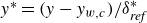 $y^*=(y-y_{w,c})/\delta ^*_{{\textit{ref}}}$
, and
$y^*=(y-y_{w,c})/\delta ^*_{{\textit{ref}}}$
, and
 $y_{w,c}$
is the
$y_{w,c}$
is the
 $y$
coordinate of the wing wall in the reference clean case.
$y$
coordinate of the wing wall in the reference clean case.
3. Base flow modifications induced by the hump
In this section, the effects of the hump on the base flow are investigated. The pressure coefficient (
 $-C_p$
) and the pressure gradient
$-C_p$
) and the pressure gradient
 $ (c_x(\partial C_p/\partial x) )$
from DNS (for both reference and hump cases) and the experiment of Rius-Vidales et al. (Reference Rius-Vidales, Morais, Westerbeek, Casacuberta, Soyler and Kotsonis2025) (for the reference case) are compared in figure 3(a,b). In the experiment, two streamwise rows of pressure taps located at
$ (c_x(\partial C_p/\partial x) )$
from DNS (for both reference and hump cases) and the experiment of Rius-Vidales et al. (Reference Rius-Vidales, Morais, Westerbeek, Casacuberta, Soyler and Kotsonis2025) (for the reference case) are compared in figure 3(a,b). In the experiment, two streamwise rows of pressure taps located at
 $24\,\%$
and
$24\,\%$
and
 $76 \,\%$
of the wing model span were used to measure the pressure. These are denoted by the lower (blue cross) and upper (red circle) rows, referring to their spanwise positions, i.e. closer to the wind tunnel bottom wall and wind tunnel top wall, respectively, not to the lower and upper wing surfaces. Note that, all panels in figure 3 are plotted based on the base flow solution
$76 \,\%$
of the wing model span were used to measure the pressure. These are denoted by the lower (blue cross) and upper (red circle) rows, referring to their spanwise positions, i.e. closer to the wind tunnel bottom wall and wind tunnel top wall, respectively, not to the lower and upper wing surfaces. Note that, all panels in figure 3 are plotted based on the base flow solution
 $\boldsymbol{u}_0$
for both reference and hump cases. The agreement of
$\boldsymbol{u}_0$
for both reference and hump cases. The agreement of
 $C_p$
and
$C_p$
and
 $\partial C_p/\partial x$
between DNS and experiment for the reference case is good. Figure 3(a,b) shows that, in the presence of the hump, the pressure is locally modified by the hump, and recovers to the reference case values rapidly downstream of the hump. Therefore, the boundary-layer flow experiences successive pressure-gradient changeovers from favourable pressure gradient (FPG;
$\partial C_p/\partial x$
between DNS and experiment for the reference case is good. Figure 3(a,b) shows that, in the presence of the hump, the pressure is locally modified by the hump, and recovers to the reference case values rapidly downstream of the hump. Therefore, the boundary-layer flow experiences successive pressure-gradient changeovers from favourable pressure gradient (FPG;
 $\partial C_p/\partial x\lt 0$
) to adverse pressure gradient (APG;
$\partial C_p/\partial x\lt 0$
) to adverse pressure gradient (APG;
 $\partial C_p/\partial x\gt 0$
) and from APG to FPG, until it recovers to the reference case pressure distribution at
$\partial C_p/\partial x\gt 0$
) and from APG to FPG, until it recovers to the reference case pressure distribution at
 $x/c_x \approx 0.2$
.
$x/c_x \approx 0.2$
.
Comparison of (a) pressure coefficient
 $(-C_p)$
and (b) pressure gradient
$(-C_p)$
and (b) pressure gradient
 $(c_x(\partial C_p/\partial x))$
between DNS (reference clean and hump cases) and the experiment of Rius-Vidales et al. (Reference Rius-Vidales, Morais, Westerbeek, Casacuberta, Soyler and Kotsonis2025). (c) Displacement thickness (
$(c_x(\partial C_p/\partial x))$
between DNS (reference clean and hump cases) and the experiment of Rius-Vidales et al. (Reference Rius-Vidales, Morais, Westerbeek, Casacuberta, Soyler and Kotsonis2025). (c) Displacement thickness (
 $\delta ^*$
) and momentum thickness (
$\delta ^*$
) and momentum thickness (
 $\theta \times 5$
). (d) Skin-friction coefficient in direction of
$\theta \times 5$
). (d) Skin-friction coefficient in direction of
 $U_t$
and
$U_t$
and
 $W_{\textit{cf}}$
. The extent of the hump is highlighted in orange and the location of its apex is marked by the vertical solid orange line at
$W_{\textit{cf}}$
. The extent of the hump is highlighted in orange and the location of its apex is marked by the vertical solid orange line at
 $x/c_x=0.15$
. The vertical black dashed lines indicate the beginning and end of the CF reversal region.
$x/c_x=0.15$
. The vertical black dashed lines indicate the beginning and end of the CF reversal region.

The effect of the hump on the boundary-layer displacement thickness
 $\delta ^*$
and momentum thickness
$\delta ^*$
and momentum thickness
 $\theta$
is shown in figure 3(c). Both
$\theta$
is shown in figure 3(c). Both
 $\delta ^*$
and
$\delta ^*$
and
 $\theta$
are mostly affected in the region where the pressure gradient is altered by the hump. Overall,
$\theta$
are mostly affected in the region where the pressure gradient is altered by the hump. Overall,
 $\delta ^*$
and
$\delta ^*$
and
 $\theta$
decrease (compared to reference case values) as the boundary layer flow accelerates over the initial part of the hump, and increase as it decelerates downstream of the hump’s apex. The boundary-layer integral quantities in the presence of the hump recover their values as for the reference case for
$\theta$
decrease (compared to reference case values) as the boundary layer flow accelerates over the initial part of the hump, and increase as it decelerates downstream of the hump’s apex. The boundary-layer integral quantities in the presence of the hump recover their values as for the reference case for
 $x/c_x \gtrsim 0.2$
.
$x/c_x \gtrsim 0.2$
.
Figure 3(d) depicts the wall skin-friction coefficient (
 $C_{\kern-1.5pt f}$
) calculated from the wall-normal shear of different velocity components. The skin friction in the direction of the outer inviscid streamline (
$C_{\kern-1.5pt f}$
) calculated from the wall-normal shear of different velocity components. The skin friction in the direction of the outer inviscid streamline (
 $C_{f,U_{t}}=( {\mu _{\infty }}/({0.5 \rho _{\infty }U_{\infty }^2}))\partial U_{t} / \partial \eta '$
, solid line) remains positive downstream of the hump. This confirms that the flow remains fully attached, and flow separation does not occur downstream of the hump. However, the skin friction in the direction of the CF velocity component (
$C_{f,U_{t}}=( {\mu _{\infty }}/({0.5 \rho _{\infty }U_{\infty }^2}))\partial U_{t} / \partial \eta '$
, solid line) remains positive downstream of the hump. This confirms that the flow remains fully attached, and flow separation does not occur downstream of the hump. However, the skin friction in the direction of the CF velocity component (
 $C_{f,W_{\textit{cf}}}=( {\mu _{\infty }}/({0.5 \rho _{\infty }U_{\infty }^2}))\partial W_{\textit{cf}} / \partial \eta '$
, dashed line) becomes negative for
$C_{f,W_{\textit{cf}}}=( {\mu _{\infty }}/({0.5 \rho _{\infty }U_{\infty }^2}))\partial W_{\textit{cf}} / \partial \eta '$
, dashed line) becomes negative for
 $0.155\lt x/c_x\lt 0.178$
, suggesting that the CF velocity component reverses its direction (i.e. CF reversal). The inception of the CF reversal region at
$0.155\lt x/c_x\lt 0.178$
, suggesting that the CF velocity component reverses its direction (i.e. CF reversal). The inception of the CF reversal region at
 $x/c_x=0.155$
(marked by the vertical black dashed line in figure 3
a–c) corresponds to where the boundary-layer flow begins to accelerate again after encountering the peak APG over the hump. This reversal extends almost to the aft end of the hump, as can be seen in figure 3(d).
$x/c_x=0.155$
(marked by the vertical black dashed line in figure 3
a–c) corresponds to where the boundary-layer flow begins to accelerate again after encountering the peak APG over the hump. This reversal extends almost to the aft end of the hump, as can be seen in figure 3(d).
The inviscid streamline angle
 $(\psi _s)$
for the reference and hump cases along the chord (see (2.3) for its definition) is shown in figure 4(a). Modifications of
$(\psi _s)$
for the reference and hump cases along the chord (see (2.3) for its definition) is shown in figure 4(a). Modifications of
 $\psi _s$
are mostly evident in the vicinity of the hump, specifically downstream of the apex of the hump and within the CF reversal region. The velocity magnitude at the boundary-layer edge (dashed lines, figure 4
a) shows the acceleration of the boundary-layer flow as it advects over the hump. The evolution of the wall-normal peak of the CF velocity component (in its nominal direction for the reference case, i.e. from
$\psi _s$
are mostly evident in the vicinity of the hump, specifically downstream of the apex of the hump and within the CF reversal region. The velocity magnitude at the boundary-layer edge (dashed lines, figure 4
a) shows the acceleration of the boundary-layer flow as it advects over the hump. The evolution of the wall-normal peak of the CF velocity component (in its nominal direction for the reference case, i.e. from
 $+z$
to
$+z$
to
 $-z$
) is shown by the solid lines in figure 4(b). The CF component experiences a significant increase in the hump case (compared with the reference case) close to the apex of the hump, which is followed by a weakening of
$-z$
) is shown by the solid lines in figure 4(b). The CF component experiences a significant increase in the hump case (compared with the reference case) close to the apex of the hump, which is followed by a weakening of
 $W_{\textit{cf}}$
in the aft part of the hump. The wall-normal peak of the CF reversal is also shown by dashed lines in the same figure. Finally, the spatial development of
$W_{\textit{cf}}$
in the aft part of the hump. The wall-normal peak of the CF reversal is also shown by dashed lines in the same figure. Finally, the spatial development of
 $U_t$
and
$U_t$
and
 $W_{\textit{cf}}$
is depicted in figure 4(c–f) for reference and hump cases. The region of reversal of CF velocity component is enclosed within the loci of
$W_{\textit{cf}}$
is depicted in figure 4(c–f) for reference and hump cases. The region of reversal of CF velocity component is enclosed within the loci of
 $W_{\textit{cf}}=0$
(white-dashed contour line). Evidently, the reversal of
$W_{\textit{cf}}=0$
(white-dashed contour line). Evidently, the reversal of
 $W_{\textit{cf}}$
occurs only in a region close to the wall.
$W_{\textit{cf}}$
occurs only in a region close to the wall.
(a) The inviscid streamline angle
 $\psi _s$
(solid lines) and velocity magnitude at the inviscid boundary-layer edge
$\psi _s$
(solid lines) and velocity magnitude at the inviscid boundary-layer edge
 $Q_e$
(dashed lines). (b) Wall-normal peak of the CF velocity component (solid lines) and reversed CF velocity component (dashed lines). Contour of
$Q_e$
(dashed lines). (b) Wall-normal peak of the CF velocity component (solid lines) and reversed CF velocity component (dashed lines). Contour of
 $U_t$
and
$U_t$
and
 $W_{\textit{cf}}$
for reference (c,e) and hump (d,f) cases. The white dashed line in (f) indicates
$W_{\textit{cf}}$
for reference (c,e) and hump (d,f) cases. The white dashed line in (f) indicates
 $W_{\textit{cf}}=0$
. In (a,b), the extent of the hump is highlighted in orange and the location of its apex is marked by the vertical orange solid line. The vertical black dashed lines in (a,b) indicate the beginning and end of the CF reversal region.
$W_{\textit{cf}}=0$
. In (a,b), the extent of the hump is highlighted in orange and the location of its apex is marked by the vertical orange solid line. The vertical black dashed lines in (a,b) indicate the beginning and end of the CF reversal region.

In figure 5, the
 $U_{t}$
and
$U_{t}$
and
 $W_{\textit{cf}}$
profiles from the reference clean and hump cases are compared at five locations along the chord. At the apex of the hump and slightly upstream, the magnitude of the CF velocity component is increased due to the presence of the hump, and the wall-normal location of its peak value is moved closer to the wall. However, just downstream of the apex of the hump, the CF velocity component profile is distorted and its direction reverses close to the wall, which causes an additional inflection point in the profile of
$W_{\textit{cf}}$
profiles from the reference clean and hump cases are compared at five locations along the chord. At the apex of the hump and slightly upstream, the magnitude of the CF velocity component is increased due to the presence of the hump, and the wall-normal location of its peak value is moved closer to the wall. However, just downstream of the apex of the hump, the CF velocity component profile is distorted and its direction reverses close to the wall, which causes an additional inflection point in the profile of
 $W_{\textit{cf}}$
in that region. Farther downstream (i.e. at
$W_{\textit{cf}}$
in that region. Farther downstream (i.e. at
 $x/c_x=0.19$
), although the CF velocity component recovers its nominal direction, its shape differs significantly compared with the reference case. However,
$x/c_x=0.19$
), although the CF velocity component recovers its nominal direction, its shape differs significantly compared with the reference case. However,
 $U_{t}$
shows a similar profile to that of the reference case at this location. Finally, for
$U_{t}$
shows a similar profile to that of the reference case at this location. Finally, for
 $x/c_x \gtrsim 0.25$
, the CF velocity component almost recovers fully to the shape corresponding to the reference case.
$x/c_x \gtrsim 0.25$
, the CF velocity component almost recovers fully to the shape corresponding to the reference case.
Profiles of
 $U_{t}$
and
$U_{t}$
and
 $W_{\textit{cf}}$
for the reference clean (black) and hump (red) cases. The profiles are obtained from the base flow
$W_{\textit{cf}}$
for the reference clean (black) and hump (red) cases. The profiles are obtained from the base flow
 $\boldsymbol{u}_0$
. Note that CF velocity component profiles are multiplied by a factor of 5 for visibility.
$\boldsymbol{u}_0$
. Note that CF velocity component profiles are multiplied by a factor of 5 for visibility.

4. Transition delay by the hump
In this section, simulation results for the low-amplitude incoming CF perturbation, cases A1-C and A1-H, are presented. First, in §§ 4.1 and 4.2, the evolution of primary stationary CF perturbation and its interaction with the hump are analysed. In § 4.3, the effects of the hump on secondary instabilities and laminar breakdown are investigated.
4.1. Effect of the hump on primary stationary CFI
Comparisons between time- and spanwise-averaged spanwise meanflow profiles (
 $\bar {w}$
) and steady disturbance profiles (
$\bar {w}$
) and steady disturbance profiles (
 $\langle \bar {w} \rangle _z$
, see (2.11)) between DNS and experiments by Rius-Vidales et al. (Reference Rius-Vidales, Morais, Westerbeek, Casacuberta, Soyler and Kotsonis2025) are shown in figure 6. Note that the total perturbation profiles from the experimental measurements are used here for comparison with the DNS data. For more details on the experimental data, the reader is referred to Rius-Vidales et al. (Reference Rius-Vidales, Morais, Westerbeek, Casacuberta, Soyler and Kotsonis2025, figure 5e). Figure 6(e) shows the chordwise evolution of wall-normal maximum of
$\langle \bar {w} \rangle _z$
, see (2.11)) between DNS and experiments by Rius-Vidales et al. (Reference Rius-Vidales, Morais, Westerbeek, Casacuberta, Soyler and Kotsonis2025) are shown in figure 6. Note that the total perturbation profiles from the experimental measurements are used here for comparison with the DNS data. For more details on the experimental data, the reader is referred to Rius-Vidales et al. (Reference Rius-Vidales, Morais, Westerbeek, Casacuberta, Soyler and Kotsonis2025, figure 5e). Figure 6(e) shows the chordwise evolution of wall-normal maximum of
 $\langle \bar {w} \rangle _z$
along the chord. Note that the experimental data along the chord are measured in
$\langle \bar {w} \rangle _z$
along the chord. Note that the experimental data along the chord are measured in
 $z$
–
$z$
–
 $y_E$
planes, where
$y_E$
planes, where
 $z$
is parallel to the leading edge and
$z$
is parallel to the leading edge and
 $y_E$
is normal to the wing surface (at
$y_E$
is normal to the wing surface (at
 $x/c_x \approx 0.15$
) in the reference configuration. This direction is held constant along the chord, making the measurement planes quasi-normal to the wing surface downstream, with the
$x/c_x \approx 0.15$
) in the reference configuration. This direction is held constant along the chord, making the measurement planes quasi-normal to the wing surface downstream, with the
 $y_E$
origin located on the wing surface.
$y_E$
origin located on the wing surface.
(a–d) Profiles of
 $\langle \bar {w} \rangle _z/w_e$
and time- and spanwise-averaged spanwise velocity component (
$\langle \bar {w} \rangle _z/w_e$
and time- and spanwise-averaged spanwise velocity component (
 $\bar {w}/w_e$
). (e) Chordwise evolution of wall-normal peak
$\bar {w}/w_e$
). (e) Chordwise evolution of wall-normal peak
 $\langle \bar {w} \rangle _z/w_e$
, for cases A1-C and A1-H. Note that experimental data are plotted along the
$\langle \bar {w} \rangle _z/w_e$
, for cases A1-C and A1-H. Note that experimental data are plotted along the
 $\eta _E$
direction, where
$\eta _E$
direction, where
 $\eta _E=y_E/\delta ^*_{{\textit{ref}}}$
. Black and red dashed lines in (e) show the peak value of
$\eta _E=y_E/\delta ^*_{{\textit{ref}}}$
. Black and red dashed lines in (e) show the peak value of
 $\langle \bar {w} \rangle _z/w_e$
obtained from the simulations without unsteady disturbances in the domain for cases A1-C and A1-H, respectively. The grey shaded area shows the region where skin friction starts to increase in DNS for case A1-C (cf. figure 11). Note that DNS and experimental profiles are normalised by local spanwise velocity component in the free stream obtained in DNS and experiments, respectively.
$\langle \bar {w} \rangle _z/w_e$
obtained from the simulations without unsteady disturbances in the domain for cases A1-C and A1-H, respectively. The grey shaded area shows the region where skin friction starts to increase in DNS for case A1-C (cf. figure 11). Note that DNS and experimental profiles are normalised by local spanwise velocity component in the free stream obtained in DNS and experiments, respectively.

From figure 6, it is clear that both the spanwise-averaged meanflow and primary CF disturbance profiles (figure 6 a–d) and the growth (figure 6 e) in DNS match very well with the experiment. It should be noted that small differences between the profiles obtained by DNS and experiment exist, and are likely caused by a combination of the measurement planes in DNS being normal to local curvature of the wall and the measurement planes in the experiments being quasi-normal to the wall, and also the use of an idealised hump shape for DNS as explained in § 2.2. However, as is shown in later sections, these minor differences do not affect the general conclusions of this work.
Steady disturbance profiles of chordwise
 $(u_{\xi })$
, wall-normal
$(u_{\xi })$
, wall-normal
 $(v_{\eta '})$
and spanwise
$(v_{\eta '})$
and spanwise
 $(w)$
components for cases A1-C (black) and A1-H (red) in DNS. Note that the disturbance profiles are calculated based on stationary perturbation field, i.e.
$(w)$
components for cases A1-C (black) and A1-H (red) in DNS. Note that the disturbance profiles are calculated based on stationary perturbation field, i.e.
 $\boldsymbol{u}^{\prime}_s$
.
$\boldsymbol{u}^{\prime}_s$
.

Figure 6(e) clearly shows the stabilisation of the stationary CF disturbances downstream of the hump in both the experiments and the DNS. To better investigate the influence of the hump on the development of CFVs, figure 7 compares the steady disturbance profiles (calculated using stationary perturbation fields
 $\boldsymbol{u}^{\prime}_s$
from DNS) for all three velocity components (
$\boldsymbol{u}^{\prime}_s$
from DNS) for all three velocity components (
 $\langle {u}^{\prime}_{\xi ,s} \rangle _z$
,
$\langle {u}^{\prime}_{\xi ,s} \rangle _z$
,
 $\langle {v}^{\prime}_{\eta ',s} \rangle _z$
and
$\langle {v}^{\prime}_{\eta ',s} \rangle _z$
and
 $\langle {w^{\prime}_s} \rangle _z$
) between cases A1-C and A1-H. A notable effect of the hump is on the shape of the spanwise and chordwise components of the disturbance in the vicinity of the hump. As the flow passes over the hump, it experiences an APG, which results in thickening of the boundary layer and increase of integral length quantities, as shown in figure 3. The effect is evident on the disturbance profiles slightly downstream of the apex of the hump (figure 7Ia,Ib), where the wall-normal location of peak
$\langle {w^{\prime}_s} \rangle _z$
) between cases A1-C and A1-H. A notable effect of the hump is on the shape of the spanwise and chordwise components of the disturbance in the vicinity of the hump. As the flow passes over the hump, it experiences an APG, which results in thickening of the boundary layer and increase of integral length quantities, as shown in figure 3. The effect is evident on the disturbance profiles slightly downstream of the apex of the hump (figure 7Ia,Ib), where the wall-normal location of peak
 $\langle {w^{\prime}_s} \rangle _z$
and
$\langle {w^{\prime}_s} \rangle _z$
and
 $\langle {u}^{\prime}_{\xi ,s} \rangle _z$
moves away from the wall compared with the reference case. As shown earlier, CF reversal occurs for
$\langle {u}^{\prime}_{\xi ,s} \rangle _z$
moves away from the wall compared with the reference case. As shown earlier, CF reversal occurs for
 $0.155\lt x/c_x\lt 0.178$
in the hump case due to the consequent acceleration–deceleration events. In this region, the disturbance profiles (
$0.155\lt x/c_x\lt 0.178$
in the hump case due to the consequent acceleration–deceleration events. In this region, the disturbance profiles (
 $\langle {w^{\prime}_s} \rangle _z$
and
$\langle {w^{\prime}_s} \rangle _z$
and
 $\langle {u}^{\prime}_{\xi ,s} \rangle _z$
) in the hump case become highly distorted compared with the reference case. The disturbance profiles within this region show a double-peak profile, as shown in figure 7(Ib) for
$\langle {u}^{\prime}_{\xi ,s} \rangle _z$
) in the hump case become highly distorted compared with the reference case. The disturbance profiles within this region show a double-peak profile, as shown in figure 7(Ib) for
 $x/c_x=0.172$
. At this station, the stronger peak is located farther away from the wall. Slightly downstream of the CF reversal region (figure 7Ic), the disturbance profiles remain highly distorted compared with the reference case, until
$x/c_x=0.172$
. At this station, the stronger peak is located farther away from the wall. Slightly downstream of the CF reversal region (figure 7Ic), the disturbance profiles remain highly distorted compared with the reference case, until
 $x/c_x\approx 0.19$
where they are approximately recovered to the shape of the reference case. At
$x/c_x\approx 0.19$
where they are approximately recovered to the shape of the reference case. At
 $x/c_x=0.2$
(figure 7IIa), the wall-normal peak value of
$x/c_x=0.2$
(figure 7IIa), the wall-normal peak value of
 $\langle \bar {u}_{\xi } \rangle _z$
is slightly higher in the hump case compared with the reference case. Interestingly, for
$\langle \bar {u}_{\xi } \rangle _z$
is slightly higher in the hump case compared with the reference case. Interestingly, for
 $x/c_x \gtrsim 0.20$
, a strong stabilisation in the primary CF perturbations occurs in the hump case, as clearly seen in figures 6 and 7(IIb–d). This long-lasting and far-downstream effect of the hump on growth of stationary CF perturbations provides important insights to the core contribution of the hump to the observed transition delay in experiments and DNS (as shown in § 4.3). In the following sections, the physical mechanisms responsible for this stabilisation are further explored.
$x/c_x \gtrsim 0.20$
, a strong stabilisation in the primary CF perturbations occurs in the hump case, as clearly seen in figures 6 and 7(IIb–d). This long-lasting and far-downstream effect of the hump on growth of stationary CF perturbations provides important insights to the core contribution of the hump to the observed transition delay in experiments and DNS (as shown in § 4.3). In the following sections, the physical mechanisms responsible for this stabilisation are further explored.
4.2. Effect of the hump on harmonics of the primary stationary CF perturbation
Spanwise harmonic modes of primary stationary CF perturbation are calculated using spanwise Fourier transform of chordwise perturbation profiles
 $u^{\prime}_{\xi ,s}$
using (2.8).
$u^{\prime}_{\xi ,s}$
using (2.8).
The amplitudes of the first four modes, i.e.
 $A_{\tilde {u}_\xi ,n\beta _0} \,(n \in [1,4])$
, for
$A_{\tilde {u}_\xi ,n\beta _0} \,(n \in [1,4])$
, for
 $0.06\lt x/c_x\lt 0.50$
are plotted in figure 8(a), where the black and red lines correspond to cases A1-C and A1-H, respectively. This figure reveals that the trend in chordwise evolution of the amplitude of the fundamental spanwise mode (
$0.06\lt x/c_x\lt 0.50$
are plotted in figure 8(a), where the black and red lines correspond to cases A1-C and A1-H, respectively. This figure reveals that the trend in chordwise evolution of the amplitude of the fundamental spanwise mode (
 $1\beta _0$
) is strongly affected in the vicinity of the hump. However, the amplitude itself does not exceed that of the reference case, except slightly upstream of the hump’s apex and for
$1\beta _0$
) is strongly affected in the vicinity of the hump. However, the amplitude itself does not exceed that of the reference case, except slightly upstream of the hump’s apex and for
 $0.19\lt x/c_x\lt 0.21$
. For
$0.19\lt x/c_x\lt 0.21$
. For
 $x/c_x\gt 0.21$
, the fundamental mode appears stabilised compared with the reference case. In contrast, higher harmonics behave notably differently in the vicinity of the hump, with a strong increase in their amplitude just downstream of the hump’s apex. Interestingly, after the localised amplification of higher harmonics, their amplitude subsequently decays to well below the corresponding reference case for more downstream locations. It is worth mentioning that the amplification of higher harmonics starts almost at the same location as the CF reversal occurs, and continues until
$x/c_x\gt 0.21$
, the fundamental mode appears stabilised compared with the reference case. In contrast, higher harmonics behave notably differently in the vicinity of the hump, with a strong increase in their amplitude just downstream of the hump’s apex. Interestingly, after the localised amplification of higher harmonics, their amplitude subsequently decays to well below the corresponding reference case for more downstream locations. It is worth mentioning that the amplification of higher harmonics starts almost at the same location as the CF reversal occurs, and continues until
 $x/c_x \approx 0.185$
, which is just downstream of the end of the CF reversal region at
$x/c_x \approx 0.185$
, which is just downstream of the end of the CF reversal region at
 $x/c_x \approx 0.178$
. Unlike the higher harmonic modes, the fundamental mode
$x/c_x \approx 0.178$
. Unlike the higher harmonic modes, the fundamental mode
 $1\beta _0$
behaves differently in the CF reversal region, and its amplitude slightly decreases in that region, as can be seen in the inset of figure 8(a).
$1\beta _0$
behaves differently in the CF reversal region, and its amplitude slightly decreases in that region, as can be seen in the inset of figure 8(a).
(a) Chordwise evolution of amplitude of the fundamental mode
 $1\beta _0$
and first three higher harmonics (
$1\beta _0$
and first three higher harmonics (
 $2\beta _0$
–
$2\beta _0$
–
 $4\beta _0$
) of
$4\beta _0$
) of
 $u^{\prime}_{\xi ,s}$
for cases A1-C (black) and A1-H (red). (b) Ratio of spatial growth rate (cf. (2.10)) of fundamental mode
$u^{\prime}_{\xi ,s}$
for cases A1-C (black) and A1-H (red). (b) Ratio of spatial growth rate (cf. (2.10)) of fundamental mode
 $1\beta _0$
of hump to reference case calculated by chordwise (
$1\beta _0$
of hump to reference case calculated by chordwise (
 $\tilde {u}_\xi$
) and spanwise (
$\tilde {u}_\xi$
) and spanwise (
 $\tilde {w}$
) Fourier coefficients. Subscripts
$\tilde {w}$
) Fourier coefficients. Subscripts
 $c$
and
$c$
and
 $h$
stand for clean (reference) and hump cases, respectively.
$h$
stand for clean (reference) and hump cases, respectively.

The ratio between the spatial chordwise growth rate (calculated using (2.10)) between cases A1-H and A1-C for the fundamental stationary mode
 $(\sigma _h/\sigma _c)_{1\beta _0}$
is shown in figure 8(b). It is evident that the growth rate of the fundamental mode downstream of the hump’s apex decreases compared with that of the reference case. In this region (
$(\sigma _h/\sigma _c)_{1\beta _0}$
is shown in figure 8(b). It is evident that the growth rate of the fundamental mode downstream of the hump’s apex decreases compared with that of the reference case. In this region (
 $0.151\lt x/c_x\lt 0.174$
), the flow experiences a strong APG (see figure 3
b), which could explain the local stabilisation of the fundamental CF mode. Thus, the fundamental mode in this region is mostly affected by the effects of the pressure gradient, towards stabilising it. However, as soon as the flow experiences the enhanced FPG at
$0.151\lt x/c_x\lt 0.174$
), the flow experiences a strong APG (see figure 3
b), which could explain the local stabilisation of the fundamental CF mode. Thus, the fundamental mode in this region is mostly affected by the effects of the pressure gradient, towards stabilising it. However, as soon as the flow experiences the enhanced FPG at
 $x/c_x=0.174$
, the growth rate of the fundamental mode increases in the hump case. The growth rate then starts to recover to the reference case value, until
$x/c_x=0.174$
, the growth rate of the fundamental mode increases in the hump case. The growth rate then starts to recover to the reference case value, until
 $x/c_x \approx 0.2$
where
$x/c_x \approx 0.2$
where
 $(\sigma _h/\sigma _c)_{1\beta _0} \approx 1$
. More downstream for
$(\sigma _h/\sigma _c)_{1\beta _0} \approx 1$
. More downstream for
 $0.2\lt x/c_x\lt 0.26$
, the chordwise growth rate of the fundamental mode in the hump case becomes less than the growth rate in the reference case, i.e.
$0.2\lt x/c_x\lt 0.26$
, the chordwise growth rate of the fundamental mode in the hump case becomes less than the growth rate in the reference case, i.e.
 $(\sigma _h/\sigma _c)_{1\beta _0} \lt 1$
, which is also observable in figure 6(e). For
$(\sigma _h/\sigma _c)_{1\beta _0} \lt 1$
, which is also observable in figure 6(e). For
 $x/c_x\gt 0.2$
, the pressure gradient is almost recovered to its values as for the reference case (figure 3
b). Thus, the lower growth rate in the hump case compared with the reference case for
$x/c_x\gt 0.2$
, the pressure gradient is almost recovered to its values as for the reference case (figure 3
b). Thus, the lower growth rate in the hump case compared with the reference case for
 $x/c_x\gt 0.2$
, which results in the far-downstream stabilising effect of the hump, can no longer be directly attributed to the local pressure gradient effects. These observations suggest that stationary CF perturbations passing over the hump may undergo topological changes due to the upstream pressure-gradient changeover from FPG to APG. These changes persist far downstream of the hump and lead to a reduced growth rate of CF perturbations compared with that in the reference case, as suggested by Rius-Vidales et al. (Reference Rius-Vidales, Morais, Westerbeek, Casacuberta, Soyler and Kotsonis2025). This positive interaction mechanism is investigated in the following section.
$x/c_x\gt 0.2$
, which results in the far-downstream stabilising effect of the hump, can no longer be directly attributed to the local pressure gradient effects. These observations suggest that stationary CF perturbations passing over the hump may undergo topological changes due to the upstream pressure-gradient changeover from FPG to APG. These changes persist far downstream of the hump and lead to a reduced growth rate of CF perturbations compared with that in the reference case, as suggested by Rius-Vidales et al. (Reference Rius-Vidales, Morais, Westerbeek, Casacuberta, Soyler and Kotsonis2025). This positive interaction mechanism is investigated in the following section.
4.2.1. Effect of the hump on the topology of primary stationary CF perturbations
Figure 9 depicts the topology of the stationary CF perturbations (
 $u_\xi$
component) at selected chordwise stations, for cases A1-C and A1-H. Note that the
$u_\xi$
component) at selected chordwise stations, for cases A1-C and A1-H. Note that the
 $z^*$
coordinate is shifted relative to the
$z^*$
coordinate is shifted relative to the
 $z$
direction to align the CFVs across different chordwise stations. As expected for the reference case, the shape and topology of perturbations are almost similar and only their amplitude increases in more downstream locations. However, the perturbations in the hump case undergo severe topological changes. At
$z$
direction to align the CFVs across different chordwise stations. As expected for the reference case, the shape and topology of perturbations are almost similar and only their amplitude increases in more downstream locations. However, the perturbations in the hump case undergo severe topological changes. At
 $x/c_x=0.17$
(figure 9IIa,IVa,VIa) where the CF reversal occurs,
$x/c_x=0.17$
(figure 9IIa,IVa,VIa) where the CF reversal occurs,
 $W_{\textit{cf}}=0$
is indicated by the green dashed line. Note that within the CF reversal region, a new inflection point appears in the CF velocity component profile, which might give rise to new inflectional primary instabilities, as shown by Westerbeek et al. (Reference Westerbeek, Casacuberta and Kotsonis2026). Interestingly, at this station for the hump case, CF perturbations near the wall experience a shear in the direction of the reversed CF velocity component (which is from −
$W_{\textit{cf}}=0$
is indicated by the green dashed line. Note that within the CF reversal region, a new inflection point appears in the CF velocity component profile, which might give rise to new inflectional primary instabilities, as shown by Westerbeek et al. (Reference Westerbeek, Casacuberta and Kotsonis2026). Interestingly, at this station for the hump case, CF perturbations near the wall experience a shear in the direction of the reversed CF velocity component (which is from −
 $z^*$
to +
$z^*$
to +
 $z^*$
direction), and the perturbations are tilted against their original tilting. This is clearly visible by the zero-phase isolines (i.e.
$z^*$
direction), and the perturbations are tilted against their original tilting. This is clearly visible by the zero-phase isolines (i.e.
 $\phi =\arctan (\operatorname {Im}{(\hat {u}_{\xi })}/\operatorname {\textit{Re}}{(\hat {u}_{\xi })} )=0)$
in figure 9 for the fundamental (row IV) and the first harmonic modes (row VI). The same topology change in the stationary CF perturbations has been observed in the experiments of Rius-Vidales et al. (Reference Rius-Vidales, Morais, Westerbeek, Casacuberta, Soyler and Kotsonis2025), and in numerical simulations of Wassermann & Kloker (Reference Wassermann and Kloker2005) investigating the effect of pressure-gradient changeover from FPG to APG. The aforementioned works point towards the formation of a new structure near the wall due to CF reversal (due to pressure-gradient changeover from FPG to APG), and possibly a new stationary inflectional instability which becomes unstable within that region (Westerbeek et al. Reference Westerbeek, Casacuberta and Kotsonis2026). Slightly downstream of the CF reversal region in case A1-H, as shown in figure 9(b) at
$\phi =\arctan (\operatorname {Im}{(\hat {u}_{\xi })}/\operatorname {\textit{Re}}{(\hat {u}_{\xi })} )=0)$
in figure 9 for the fundamental (row IV) and the first harmonic modes (row VI). The same topology change in the stationary CF perturbations has been observed in the experiments of Rius-Vidales et al. (Reference Rius-Vidales, Morais, Westerbeek, Casacuberta, Soyler and Kotsonis2025), and in numerical simulations of Wassermann & Kloker (Reference Wassermann and Kloker2005) investigating the effect of pressure-gradient changeover from FPG to APG. The aforementioned works point towards the formation of a new structure near the wall due to CF reversal (due to pressure-gradient changeover from FPG to APG), and possibly a new stationary inflectional instability which becomes unstable within that region (Westerbeek et al. Reference Westerbeek, Casacuberta and Kotsonis2026). Slightly downstream of the CF reversal region in case A1-H, as shown in figure 9(b) at
 $x/c_x=0.18$
, the fundamental mode near the wall is still oriented in the direction against the original orientation of CF perturbation due to inertia and upstream history of the flow, but the tilting is less than previous stations.
$x/c_x=0.18$
, the fundamental mode near the wall is still oriented in the direction against the original orientation of CF perturbation due to inertia and upstream history of the flow, but the tilting is less than previous stations.
(a–d) Chordwise velocity component of total CF perturbation (
 $u^{\prime}_{\xi ,s}=\bar {u}_{\xi }-u_{\xi ,0}$
) (rows I, II), fundamental mode (rows III, IV) and first higher harmonic mode (rows V, VI). Rows (I, III, V) correspond to case A1-C and rows (II, IV, VI) to case A1-H. The black lines show nine equally spaced isolines of the time-averaged chordwise velocity component in the interval of
$u^{\prime}_{\xi ,s}=\bar {u}_{\xi }-u_{\xi ,0}$
) (rows I, II), fundamental mode (rows III, IV) and first higher harmonic mode (rows V, VI). Rows (I, III, V) correspond to case A1-C and rows (II, IV, VI) to case A1-H. The black lines show nine equally spaced isolines of the time-averaged chordwise velocity component in the interval of
 $[0,0.95u_\xi ^{\textit{max}}]$
. Green dashed line at
$[0,0.95u_\xi ^{\textit{max}}]$
. Green dashed line at
 $x/c_x=0.17$
(rows II, IV, VI) denotes
$x/c_x=0.17$
(rows II, IV, VI) denotes
 $W_{\textit{cf}}=0$
for the hump case. The black dashed lines show constant zero-phase (
$W_{\textit{cf}}=0$
for the hump case. The black dashed lines show constant zero-phase (
 $\phi =0$
) isolines of perturbations. Panels are not drawn to scale.
$\phi =0$
) isolines of perturbations. Panels are not drawn to scale.

(a) Constant-phase (
 $\phi =0$
) isolines of fundamental mode
$\phi =0$
) isolines of fundamental mode
 $\hat {u}_{\xi ,1\beta _0}$
for cases A1-C (black) and A1-H (red) at several chordwise locations. (b) Difference between
$\hat {u}_{\xi ,1\beta _0}$
for cases A1-C (black) and A1-H (red) at several chordwise locations. (b) Difference between
 $z$
coordinate of zero-phase isolines of hump and reference cases close to the wall (
$z$
coordinate of zero-phase isolines of hump and reference cases close to the wall (
 $\Delta z^*$
). Contour of the integrand of the total production term calculated for fundamental mode for case (c) A1-C and (d) A1-H. (e) Chordwise evolution of the wall-normal integral of the integrand of the production term (
$\Delta z^*$
). Contour of the integrand of the total production term calculated for fundamental mode for case (c) A1-C and (d) A1-H. (e) Chordwise evolution of the wall-normal integral of the integrand of the production term (
 $\mathcal{I}_{\mathcal{P}_{1\beta _0}}$
) for case A1-C and A1-H. Here
$\mathcal{I}_{\mathcal{P}_{1\beta _0}}$
) for case A1-C and A1-H. Here
 $\mathcal{I}_{\mathcal{P}_{1\beta _0}}=0$
and
$\mathcal{I}_{\mathcal{P}_{1\beta _0}}=0$
and
 $W_{\textit{cf}}=0$
are indicated by green and black dashed contour lines in (d), respectively. The vertical black dashed lines in (b,e) show the boundaries of the CF reversal region, while the hump region is shaded in orange, and the orange vertical solid line marks its apex location. Panels (c,d) are not drawn to scale.
$W_{\textit{cf}}=0$
are indicated by green and black dashed contour lines in (d), respectively. The vertical black dashed lines in (b,e) show the boundaries of the CF reversal region, while the hump region is shaded in orange, and the orange vertical solid line marks its apex location. Panels (c,d) are not drawn to scale.

To qualitatively characterise how the tilting of stationary CF perturbations changes as the boundary-layer flow advects over the hump, constant-phase isolines
 $(\phi =0)$
of
$(\phi =0)$
of
 $\hat {u}_{\xi ,1\beta _0}$
at several locations are compared between the reference and hump cases. For this comparison, the primary mode isolines for the hump case are shifted in the
$\hat {u}_{\xi ,1\beta _0}$
at several locations are compared between the reference and hump cases. For this comparison, the primary mode isolines for the hump case are shifted in the
 $z$
direction such that the
$z$
direction such that the
 $z$
coordinate of the zero-phase isoline in the free stream matches that of the reference case. The shifted
$z$
coordinate of the zero-phase isoline in the free stream matches that of the reference case. The shifted
 $z$
coordinates for reference and hump cases are denoted by
$z$
coordinates for reference and hump cases are denoted by
 $z_c^*$
and
$z_c^*$
and
 $z_h^*$
, respectively. The results are shown in figure 10(a). The difference between the
$z_h^*$
, respectively. The results are shown in figure 10(a). The difference between the
 $z$
coordinates of the phase profiles at the first grid point off the wall, i.e.
$z$
coordinates of the phase profiles at the first grid point off the wall, i.e.
 $\Delta z^*=(z^*_h-z^*_c)_{(\phi =0,\eta '=0^+)}/\lambda _z$
, is depicted in figure 10(b). As evident in figure 10(a,b), the tilting of the classical shape of the CF perturbation occurs in the hump case over and downstream of the hump. From the initiation of the CF reversal region,
$\Delta z^*=(z^*_h-z^*_c)_{(\phi =0,\eta '=0^+)}/\lambda _z$
, is depicted in figure 10(b). As evident in figure 10(a,b), the tilting of the classical shape of the CF perturbation occurs in the hump case over and downstream of the hump. From the initiation of the CF reversal region,
 $\Delta z^*$
increases until it reaches its peak value at approximately the chordwise location of maximum CF reversal. Downstream of that point,
$\Delta z^*$
increases until it reaches its peak value at approximately the chordwise location of maximum CF reversal. Downstream of that point,
 $\Delta z^*$
decreases as the peak value of the CF reversal reduces, and, consequently, the CF perturbation begins to recover its original shape. Notably, downstream of
$\Delta z^*$
decreases as the peak value of the CF reversal reduces, and, consequently, the CF perturbation begins to recover its original shape. Notably, downstream of
 $x/c_x=0.2$
where the pressure gradient is almost recovered to the value of the reference case and
$x/c_x=0.2$
where the pressure gradient is almost recovered to the value of the reference case and
 $\Delta z^*\approx 0$
, the structure (and orientation) of the stationary CF perturbation continues to change, and only recovers to reference case conditions at
$\Delta z^*\approx 0$
, the structure (and orientation) of the stationary CF perturbation continues to change, and only recovers to reference case conditions at
 $x/c_x \approx 0.25$
. By comparing figures 10(b) and 8, it is clear that downstream of the hump, where
$x/c_x \approx 0.25$
. By comparing figures 10(b) and 8, it is clear that downstream of the hump, where
 $\Delta z^*$
is decreasing, the chordwise growth rate in the hump case decreases until it becomes lower than that in the reference case, i.e.
$\Delta z^*$
is decreasing, the chordwise growth rate in the hump case decreases until it becomes lower than that in the reference case, i.e.
 $ (\sigma _h/\sigma _c)_{1\beta _0}\lt 1$
.
$ (\sigma _h/\sigma _c)_{1\beta _0}\lt 1$
.
4.2.2. Energy budget analysis
In this section, transfer of energy between the base flow
 $\boldsymbol{u}_0$
and stationary CF perturbations is studied using the Reynolds–Orr equation, as explained in § 2.6.
$\boldsymbol{u}_0$
and stationary CF perturbations is studied using the Reynolds–Orr equation, as explained in § 2.6.
Figures 10(c) and 10(d) depict the integrand of the production term (
 $\mathcal{I}_{\mathcal{P}_{1\beta _0}}$
; see (2.12)) for cases A1-C and A1-H, respectively. The green dashed contour lines in figure 10(d) depict
$\mathcal{I}_{\mathcal{P}_{1\beta _0}}$
; see (2.12)) for cases A1-C and A1-H, respectively. The green dashed contour lines in figure 10(d) depict
 $\mathcal{I}_{\mathcal{P}_{1\beta _0}}=0$
. It is clear that in the hump case and close to the wall, there are local regions of negative production for
$\mathcal{I}_{\mathcal{P}_{1\beta _0}}=0$
. It is clear that in the hump case and close to the wall, there are local regions of negative production for
 $0.2\lt x/c_x\lt 0.24$
. This entails that within that area, the kinetic energy production term has a local stabilising effect, and the flow of kinetic energy is from the perturbation field to the base flow.
$0.2\lt x/c_x\lt 0.24$
. This entails that within that area, the kinetic energy production term has a local stabilising effect, and the flow of kinetic energy is from the perturbation field to the base flow.
The wall-normal integral of the integrand in (2.12) is depicted in figure 10(e). As expected for a locally unstable CFI, the production term in case A1-C (black line) increases monotonically. However, in case A1-H (red line) and over the hump, the term is strongly affected by the hump. Reversal of sign in the local production term (
 $\mathcal{I}_{\mathcal{P}_{1\beta _0}}\lt 0$
) in the hump case occurs where
$\mathcal{I}_{\mathcal{P}_{1\beta _0}}\lt 0$
) in the hump case occurs where
 $\Delta z^*\lt 0$
(figure 10
b). Furthermore, as shown in figure 10(e), a plateau is observed for
$\Delta z^*\lt 0$
(figure 10
b). Furthermore, as shown in figure 10(e), a plateau is observed for
 $0.19 \lt x/c_x \lt 0.22$
in the chordwise evolution of the wall-normal integral of
$0.19 \lt x/c_x \lt 0.22$
in the chordwise evolution of the wall-normal integral of
 $\mathcal{I}_{\mathcal{P}_{1\beta _0}}$
in the hump case. This plateau region corresponds to the spatial region where
$\mathcal{I}_{\mathcal{P}_{1\beta _0}}$
in the hump case. This plateau region corresponds to the spatial region where
 $\Delta z^*$
approaches zero and becomes negative until it reaches its peak negative value at
$\Delta z^*$
approaches zero and becomes negative until it reaches its peak negative value at
 $x/c_x \approx 0.22$
(figure 10
b). This corresponds to the region where the stationary CF perturbation is deviating from its classical modal structure (cf. figure 10
a,b). Analysis of the four terms (
$x/c_x \approx 0.22$
(figure 10
b). This corresponds to the region where the stationary CF perturbation is deviating from its classical modal structure (cf. figure 10
a,b). Analysis of the four terms (
 $I_1{-}I_4$
; see (2.14)) which contribute to the total production term reveals that all terms except the lift-up term (
$I_1{-}I_4$
; see (2.14)) which contribute to the total production term reveals that all terms except the lift-up term (
 $I_2$
) are negligible (details not shown here), leading to
$I_2$
) are negligible (details not shown here), leading to
 $\mathcal{P}_{1\beta _0} \approx I_2$
. These findings suggest that, for
$\mathcal{P}_{1\beta _0} \approx I_2$
. These findings suggest that, for
 $0.2\lt x/c_x\lt 0.24$
and in the absence of direct pressure-gradient effects (i.e. pressure gradient recovered reference case values), energy extraction of the perturbation field from the base flow becomes less efficient. This inefficiency arises due to a weaker lift-up effect as the perturbations tilt in the downstream region of the hump (cf. figures 9 and 10
b). The results indicate that, when the topology of the stationary CF perturbation deviates from its classical modal structure, the perturbations tend to reorganise rather than grow. In the present case, this leads to a reduced growth rate of perturbations compared with that in the reference case for
$0.2\lt x/c_x\lt 0.24$
and in the absence of direct pressure-gradient effects (i.e. pressure gradient recovered reference case values), energy extraction of the perturbation field from the base flow becomes less efficient. This inefficiency arises due to a weaker lift-up effect as the perturbations tilt in the downstream region of the hump (cf. figures 9 and 10
b). The results indicate that, when the topology of the stationary CF perturbation deviates from its classical modal structure, the perturbations tend to reorganise rather than grow. In the present case, this leads to a reduced growth rate of perturbations compared with that in the reference case for
 $x/c_x \gt 0.2$
. The present results confirm the hump stabilisation mechanism of the primary CFI proposed by Rius-Vidales et al. (Reference Rius-Vidales, Morais, Westerbeek, Casacuberta, Soyler and Kotsonis2025) and further analysed in Westerbeek et al. (Reference Westerbeek, Casacuberta and Kotsonis2026).
$x/c_x \gt 0.2$
. The present results confirm the hump stabilisation mechanism of the primary CFI proposed by Rius-Vidales et al. (Reference Rius-Vidales, Morais, Westerbeek, Casacuberta, Soyler and Kotsonis2025) and further analysed in Westerbeek et al. (Reference Westerbeek, Casacuberta and Kotsonis2026).
4.3. Effect of the hump on secondary CFI modes and laminar breakdown
(a) Time- and span-averaged wall skin-friction coefficient for cases A1-C and A1-H. The blue and grey shaded areas indicate the approximate transition region in the experiment of Rius-Vidales et al. (Reference Rius-Vidales, Morais, Westerbeek, Casacuberta, Soyler and Kotsonis2025, figure 2) and in DNS for the reference case, respectively. Time-averaged skin-friction coefficient for cases (b) A1-C and (c) A1-H in the range of
 $[0{-}3]\times 10^{-3}$
. The orange shaded area in (a) shows the extent of the hump, while the orange solid line marks the location of the hump’s apex. Note that, in (b,c) two duplicate spanwise periods of the simulation domain are used for ease of visualisation. Panels (b,c) are not drawn to scale.
$[0{-}3]\times 10^{-3}$
. The orange shaded area in (a) shows the extent of the hump, while the orange solid line marks the location of the hump’s apex. Note that, in (b,c) two duplicate spanwise periods of the simulation domain are used for ease of visualisation. Panels (b,c) are not drawn to scale.

Figure 11(a) depicts the time- and spanwise-averaged wall skin-friction coefficient
 $C_{\kern-1.5pt f}$
along the chord for cases A1-C and A1-H, whereas figure 11(b,c) depicts the time-averaged skin-friction coefficient. The blue shaded area indicates the approximate transition region measured in the experiments of Rius-Vidales et al. (Reference Rius-Vidales, Morais, Westerbeek, Casacuberta, Soyler and Kotsonis2025) for the reference case, which shows a close agreement with the transition region in the DNS for case A1-C (grey shaded region in figure 11
a). Note that the transition region in the DNS is identified from figure 11(a), where
$C_{\kern-1.5pt f}$
along the chord for cases A1-C and A1-H, whereas figure 11(b,c) depicts the time-averaged skin-friction coefficient. The blue shaded area indicates the approximate transition region measured in the experiments of Rius-Vidales et al. (Reference Rius-Vidales, Morais, Westerbeek, Casacuberta, Soyler and Kotsonis2025) for the reference case, which shows a close agreement with the transition region in the DNS for case A1-C (grey shaded region in figure 11
a). Note that the transition region in the DNS is identified from figure 11(a), where
 $ C_{\kern-1.5pt f}$
begins to increase (see the grey shaded region in figure 11
a). In case A1-H, in agreement with the experiments, no transition to turbulence is observed in the simulation domain for
$ C_{\kern-1.5pt f}$
begins to increase (see the grey shaded region in figure 11
a). In case A1-H, in agreement with the experiments, no transition to turbulence is observed in the simulation domain for
 $x/c_x\lt 0.69$
, which shows the success of the hump in delaying the transition for the present conditions.
$x/c_x\lt 0.69$
, which shows the success of the hump in delaying the transition for the present conditions.
Figure 12 shows the intensity of temporal fluctuations (i.e. standard deviation) of
 $u_\xi$
for case A1-C (row I) and A1-H (row II) at several selected
$u_\xi$
for case A1-C (row I) and A1-H (row II) at several selected
 $z{-}\eta$
planes along the chord. Time signals are collected at a fixed sampling frequency of 50 kHz from the simulations, and total numbers of 4352 and 3584 samples are collected for reference and hump cases, respectively. Initially, the stationary CF perturbations are relatively weak, causing only slight distortion of the boundary layer, and fluctuations can only be seen close to the wall. At
$z{-}\eta$
planes along the chord. Time signals are collected at a fixed sampling frequency of 50 kHz from the simulations, and total numbers of 4352 and 3584 samples are collected for reference and hump cases, respectively. Initially, the stationary CF perturbations are relatively weak, causing only slight distortion of the boundary layer, and fluctuations can only be seen close to the wall. At
 $x/c_x=0.2$
in the hump case (figure 12IIa), the amplitude of fluctuations close to the wall is noticeably higher compared with the reference case (figure 12Ia); however, still very weak (
$x/c_x=0.2$
in the hump case (figure 12IIa), the amplitude of fluctuations close to the wall is noticeably higher compared with the reference case (figure 12Ia); however, still very weak (
 ${\approx} 0.4 \,\%$
of
${\approx} 0.4 \,\%$
of
 $Q_{{\textit{ref}}}$
). Further downstream, the boundary layer becomes highly distorted as stationary CF perturbations become stronger. At these stations, in case A1-C, at the inner side of upwelling region of the CFV (IU in figure 12Ib,c), strong fluctuations can be observed; however, for case A1-H (figure 12IIb,c) these are much weaker. At
$Q_{{\textit{ref}}}$
). Further downstream, the boundary layer becomes highly distorted as stationary CF perturbations become stronger. At these stations, in case A1-C, at the inner side of upwelling region of the CFV (IU in figure 12Ib,c), strong fluctuations can be observed; however, for case A1-H (figure 12IIb,c) these are much weaker. At
 $x/c_x=0.4$
, velocity fluctuations in case A1-C are getting stronger at the outer side of the upwelling region of the CFV (OU in figure 12Ic). Also, weaker fluctuations can be observed at the upper part of the CFV and away from the wall. However, in case A1-H (figure 12IIc), no notable fluctuations are observed either at the outer side of the upwelling region of the vortex, or at its upper part away from the wall. Finally, the boundary-layer flow becomes transitional in case A1-C (figure 12Id), as indicated by the increase in wall friction coefficient shown in figure 11(a). However, for case A1-H, flow remains laminar with no significant sign of velocity fluctuations in regions rather than close to the wall (figure 12IId).
$x/c_x=0.4$
, velocity fluctuations in case A1-C are getting stronger at the outer side of the upwelling region of the CFV (OU in figure 12Ic). Also, weaker fluctuations can be observed at the upper part of the CFV and away from the wall. However, in case A1-H (figure 12IIc), no notable fluctuations are observed either at the outer side of the upwelling region of the vortex, or at its upper part away from the wall. Finally, the boundary-layer flow becomes transitional in case A1-C (figure 12Id), as indicated by the increase in wall friction coefficient shown in figure 11(a). However, for case A1-H, flow remains laminar with no significant sign of velocity fluctuations in regions rather than close to the wall (figure 12IId).
(a–d) Temporal fluctuations of chordwise velocity component (
 $u_{\xi ,{\textit{STD}}}/Q_{{\textit{ref}}}$
) for case A1-C (row I) and case A1-H (row II). The white lines show nine equally spaced isolines of the time-averaged chordwise velocity component in the interval of
$u_{\xi ,{\textit{STD}}}/Q_{{\textit{ref}}}$
) for case A1-C (row I) and case A1-H (row II). The white lines show nine equally spaced isolines of the time-averaged chordwise velocity component in the interval of
 $[0,0.95u_\xi ^{\textit{max}}]$
. Panels are not drawn to scale.
$[0,0.95u_\xi ^{\textit{max}}]$
. Panels are not drawn to scale.

The presence of high velocity fluctuations at the outer side of the upwelling region of the CFV and away from the wall are indicators of type I (
 $z$
-type) and type II (
$z$
-type) and type II (
 $y$
-type) (Malik et al. Reference Malik, Li and Chang1996, Reference Malik, Li, Choudhari and Chang1999; Wassermann & Kloker Reference Wassermann and Kloker2003) secondary CFI modes, respectively. Thus, the observed differences between velocity fluctuations in the two cases, especially on the outer side of the upwelling region of the CFV, suggest that in case A1-H, the interaction between the hump and the stationary CFVs leads to a substantial modification in the development of high-frequency secondary CFI modes. In the following section, the development of secondary CFI modes in both cases is analysed in detail.
$y$
-type) (Malik et al. Reference Malik, Li and Chang1996, Reference Malik, Li, Choudhari and Chang1999; Wassermann & Kloker Reference Wassermann and Kloker2003) secondary CFI modes, respectively. Thus, the observed differences between velocity fluctuations in the two cases, especially on the outer side of the upwelling region of the CFV, suggest that in case A1-H, the interaction between the hump and the stationary CFVs leads to a substantial modification in the development of high-frequency secondary CFI modes. In the following section, the development of secondary CFI modes in both cases is analysed in detail.
4.3.1. Spatial organisation of secondary instabilities
To segregate the different types of secondary CFI modes which develop in the present flow, spectral proper orthogonal decomposition (SPOD) (Towne, Schmidt & Colonius Reference Towne, Schmidt and Colonius2018) is used. This method aids in isolating the temporally and spatially correlated coherent structures from the unsteady simulation data. For case A1-C, 4352 three-dimensional snapshots of all three velocity components, i.e.
 $u_\xi ,\ v_{\eta '}$
and
$u_\xi ,\ v_{\eta '}$
and
 $w$
(collected at a sampling frequency of 50 kHz), for
$w$
(collected at a sampling frequency of 50 kHz), for
 $0.355\lt x/c_x\lt 0.468$
(slightly upstream of transition location) are divided into 16 blocks (with 50 % overlap), resulting in a frequency bin (
$0.355\lt x/c_x\lt 0.468$
(slightly upstream of transition location) are divided into 16 blocks (with 50 % overlap), resulting in a frequency bin (
 $\Delta f$
) equal to 97.7 Hz. For case A1-H, 3584 snapshots within the range
$\Delta f$
) equal to 97.7 Hz. For case A1-H, 3584 snapshots within the range
 $0.43\lt x/c_x\lt 0.6$
are divided into 13 blocks, with the same overlap and frequency bin as for the reference case. Figure 13 shows the leading SPOD mode energy spectrum. The chosen number of snapshots, blocks and overlaps of the blocks leads to converged SPOD spectra for both cases. The low-frequency parts of the spectrum in both cases are very similar and show high energy in the frequency band of
$0.43\lt x/c_x\lt 0.6$
are divided into 13 blocks, with the same overlap and frequency bin as for the reference case. Figure 13 shows the leading SPOD mode energy spectrum. The chosen number of snapshots, blocks and overlaps of the blocks leads to converged SPOD spectra for both cases. The low-frequency parts of the spectrum in both cases are very similar and show high energy in the frequency band of
 ${\textit{BP}}_{\textit{III}} \in [350{-}750]$
Hz. However, for the energy associated with high-frequency parts of the spectrum, significant differences can be observed. In the reference case, two clear regions of high energy can be observed in frequency bands of
${\textit{BP}}_{\textit{III}} \in [350{-}750]$
Hz. However, for the energy associated with high-frequency parts of the spectrum, significant differences can be observed. In the reference case, two clear regions of high energy can be observed in frequency bands of
 ${\textit{BP}}_{I} \in [4000{-}5500]$
Hz and
${\textit{BP}}_{I} \in [4000{-}5500]$
Hz and
 ${\textit{BP}}_{\textit{II}} \in [7000{-}8500]$
Hz. The increase in energy can be observed in the hump case for
${\textit{BP}}_{\textit{II}} \in [7000{-}8500]$
Hz. The increase in energy can be observed in the hump case for
 ${\textit{BP}}_{\textit{II}} \in [7000{-}8500]$
, although it is much less pronounced.
${\textit{BP}}_{\textit{II}} \in [7000{-}8500]$
, although it is much less pronounced.
Leading SPOD mode spectra (solid lines) for cases A1-C and A1-H. The dashed lines represent the sum of the energy of all SPOD modes for each frequency. The purple shaded areas indicate frequency bands of
 ${\textit{BP}}_{\textit{III}}\in [350{-}750]$
,
${\textit{BP}}_{\textit{III}}\in [350{-}750]$
,
 ${\textit{BP}}_{I}\in [4000{-}5500]$
and
${\textit{BP}}_{I}\in [4000{-}5500]$
and
 ${\textit{BP}}_{\textit{II}}\in [7000{-}8500]$
Hz.
${\textit{BP}}_{\textit{II}}\in [7000{-}8500]$
Hz.

The dominant frequency bands obtained by SPOD are used to filter the velocity fluctuations to identify the secondary instability mode corresponding to each frequency band. To do this, following Serpieri & Kotsonis (Reference Serpieri and Kotsonis2016), chordwise velocity fields (
 $u_\xi$
) are band-pass-filtered for both the reference and hump cases using a zero-phase eighth-order Butterworth filter, where the three frequency bands found using SPOD are used.
$u_\xi$
) are band-pass-filtered for both the reference and hump cases using a zero-phase eighth-order Butterworth filter, where the three frequency bands found using SPOD are used.
Contours of normalised root mean square of band-pass-filtered chordwise velocity fluctuation fields for (a) case A1-C:
 ${\textit{BP}}_{\textit{III}}$
(I),
${\textit{BP}}_{\textit{III}}$
(I),
 ${\textit{BP}}_{I}$
(II),
${\textit{BP}}_{I}$
(II),
 ${\textit{BP}}_{\textit{II}}$
(III) at
${\textit{BP}}_{\textit{II}}$
(III) at
 $x/c_x=0.4$
, and
$x/c_x=0.4$
, and
 $f\gt 12\,000$
Hz at
$f\gt 12\,000$
Hz at
 $x/c_x=0.458$
(IV) corresponds to high-frequency fluctuations. For (b) case A1-H:
$x/c_x=0.458$
(IV) corresponds to high-frequency fluctuations. For (b) case A1-H:
 ${\textit{BP}}_{\textit{III}}$
(I),
${\textit{BP}}_{\textit{III}}$
(I),
 ${\textit{BP}}_{I}$
(II),
${\textit{BP}}_{I}$
(II),
 ${\textit{BP}}_{\textit{II}}$
(III) at
${\textit{BP}}_{\textit{II}}$
(III) at
 $x/c_x=0.55$
. The green lines show isolines of
$x/c_x=0.55$
. The green lines show isolines of
 $0.6(\partial u_{\xi } / \partial z)^{\textit{max}}$
in (Ia,Ib),
$0.6(\partial u_{\xi } / \partial z)^{\textit{max}}$
in (Ia,Ib),
 $0.4(\partial u_{\xi } / \partial z)^{min}$
in (IIa,IVa) and
$0.4(\partial u_{\xi } / \partial z)^{min}$
in (IIa,IVa) and
 $0.05(\partial u_{\xi } / \partial \eta ')^{\textit{max}}$
in (IIIa,IIb,IIIb). The superscripts ‘max’ and ‘min’ denote the extrema at each respective location. The white lines show nine equally spaced isolines of the time-averaged chordwise velocity component in the interval of
$0.05(\partial u_{\xi } / \partial \eta ')^{\textit{max}}$
in (IIIa,IIb,IIIb). The superscripts ‘max’ and ‘min’ denote the extrema at each respective location. The white lines show nine equally spaced isolines of the time-averaged chordwise velocity component in the interval of
 $[0,0.95u_\xi ^{\textit{max}}]$
. Two repeat spanwise periods of the simulation domain are used for visualisation. Panels are not drawn to scale.
$[0,0.95u_\xi ^{\textit{max}}]$
. Two repeat spanwise periods of the simulation domain are used for visualisation. Panels are not drawn to scale.

Figure 14 shows the root mean square of band-pass-filtered
 $u_\xi$
fluctuation field (i.e.
$u_\xi$
fluctuation field (i.e.
 $u^{\prime}_{\xi ,BP}$
), for case A1-C at
$u^{\prime}_{\xi ,BP}$
), for case A1-C at
 $x/c_x=0.4$
(figure 14Ia,IIa,IIIa) and case A1-H at
$x/c_x=0.4$
(figure 14Ia,IIa,IIIa) and case A1-H at
 $x/c_x=0.55$
(figure 14Ib,IIb,IIIb). To better visualise the spatial structure of the fluctuations, each panel is normalised by its respective maximum value of the velocity fluctuation. From figure 14(Ia) it is clear that for the reference case, the velocity fluctuations corresponding to the low-frequency mode (
$x/c_x=0.55$
(figure 14Ib,IIb,IIIb). To better visualise the spatial structure of the fluctuations, each panel is normalised by its respective maximum value of the velocity fluctuation. From figure 14(Ia) it is clear that for the reference case, the velocity fluctuations corresponding to the low-frequency mode (
 ${\textit{BP}}_{\textit{III}}$
) are located at the inner side of upwelling region (IU in figure 14Ia) of the CFV, and corresponds to type III secondary CFI mode (Serpieri & Kotsonis Reference Serpieri and Kotsonis2016). This region coincides with the region of local maximum spanwise shear of the flow, as shown in figure 14(Ia) by the green solid line (i.e.
${\textit{BP}}_{\textit{III}}$
) are located at the inner side of upwelling region (IU in figure 14Ia) of the CFV, and corresponds to type III secondary CFI mode (Serpieri & Kotsonis Reference Serpieri and Kotsonis2016). This region coincides with the region of local maximum spanwise shear of the flow, as shown in figure 14(Ia) by the green solid line (i.e.
 $0.6(\partial u_{\xi } / \partial z)^{\textit{max}}$
). The velocity fluctuations corresponding to
$0.6(\partial u_{\xi } / \partial z)^{\textit{max}}$
). The velocity fluctuations corresponding to
 ${\textit{BP}}_{I}$
are located at the outer side of the upwelling (OU in figure 14IIa) region of the CFV, and corresponds to type I secondary CFI mode. This region coincides with the region of local minimum of spanwise shear, as shown in figure 14(IIa) by the green solid line (i.e.
${\textit{BP}}_{I}$
are located at the outer side of the upwelling (OU in figure 14IIa) region of the CFV, and corresponds to type I secondary CFI mode. This region coincides with the region of local minimum of spanwise shear, as shown in figure 14(IIa) by the green solid line (i.e.
 $0.4(\partial u_{\xi } / \partial z)^{min}$
). Finally, the velocity fluctuations corresponding to
$0.4(\partial u_{\xi } / \partial z)^{min}$
). Finally, the velocity fluctuations corresponding to
 ${\textit{BP}}_{\textit{II}}$
are located at the top of the CFV, and are associated with type II secondary CFI. It appears in the region of local maximum of wall-normal shear, as shown in figure 14(IIIa) by the green solid line. Under similar (though not identical) free-stream conditions and for the same wing model, Serpieri & Kotsonis (Reference Serpieri and Kotsonis2016) identified frequency bands of (5000–6000), (7000–8000) and (350–550) Hz for type I, type II and type III secondary CFI modes, respectively. The frequency bands determined using SPOD in the present study align closely with the identified frequency bands obtained in the experiments of Serpieri & Kotsonis (Reference Serpieri and Kotsonis2016). To identify the mode responsible for the onset of the laminar–turbulent transition in the reference case, following Rius-Vidales & Kotsonis (Reference Rius-Vidales and Kotsonis2022), velocity fields are high-pass-filtered, with a cutoff frequency of
${\textit{BP}}_{\textit{II}}$
are located at the top of the CFV, and are associated with type II secondary CFI. It appears in the region of local maximum of wall-normal shear, as shown in figure 14(IIIa) by the green solid line. Under similar (though not identical) free-stream conditions and for the same wing model, Serpieri & Kotsonis (Reference Serpieri and Kotsonis2016) identified frequency bands of (5000–6000), (7000–8000) and (350–550) Hz for type I, type II and type III secondary CFI modes, respectively. The frequency bands determined using SPOD in the present study align closely with the identified frequency bands obtained in the experiments of Serpieri & Kotsonis (Reference Serpieri and Kotsonis2016). To identify the mode responsible for the onset of the laminar–turbulent transition in the reference case, following Rius-Vidales & Kotsonis (Reference Rius-Vidales and Kotsonis2022), velocity fields are high-pass-filtered, with a cutoff frequency of
 $f_c=12$
kHz. The root mean square of high-pass-filtered
$f_c=12$
kHz. The root mean square of high-pass-filtered
 $u_\xi$
fluctuation field is depicted in figure 14(IVa) at
$u_\xi$
fluctuation field is depicted in figure 14(IVa) at
 $x/c_x=0.458$
, for case A1-C. The presence of very high-frequency fluctuations (indicative of turbulent fluctuations) in the outer part of the upwelling region of the CFV, coinciding with a local region of minimum spanwise gradients, suggests that the breakdown of type I secondary CFI mode triggers the transition to turbulence in case A1-C. This is in line with the previous measurements on the same swept-wing model, under similar (though not identical) flow conditions (Serpieri & Kotsonis Reference Serpieri and Kotsonis2016).
$x/c_x=0.458$
, for case A1-C. The presence of very high-frequency fluctuations (indicative of turbulent fluctuations) in the outer part of the upwelling region of the CFV, coinciding with a local region of minimum spanwise gradients, suggests that the breakdown of type I secondary CFI mode triggers the transition to turbulence in case A1-C. This is in line with the previous measurements on the same swept-wing model, under similar (though not identical) flow conditions (Serpieri & Kotsonis Reference Serpieri and Kotsonis2016).
Due to the strong stabilising effect of the hump and the resulting delay in the transition process, in case A1-H, the topology of secondary CFI modes is qualitatively inspected at a more downstream location of
 $x/c_x=0.55$
. In the hump case, the fluctuations corresponding to
$x/c_x=0.55$
. In the hump case, the fluctuations corresponding to
 ${\textit{BP}}_{\textit{III}}$
are located at the inner region of the upwelling part of the CFV, indicative of type III secondary CFI mode. However, the fluctuations corresponding to both
${\textit{BP}}_{\textit{III}}$
are located at the inner region of the upwelling part of the CFV, indicative of type III secondary CFI mode. However, the fluctuations corresponding to both
 ${\textit{BP}}_{I}$
and
${\textit{BP}}_{I}$
and
 ${\textit{BP}}_{\textit{II}}$
in the hump case are located at the top of the vortex and away from the wall. This suggests that only type II and type III secondary CFI modes are present in the hump case, and type I secondary instability appears to be stabilised as a result of the interaction of the CFVs with the hump.
${\textit{BP}}_{\textit{II}}$
in the hump case are located at the top of the vortex and away from the wall. This suggests that only type II and type III secondary CFI modes are present in the hump case, and type I secondary instability appears to be stabilised as a result of the interaction of the CFVs with the hump.
4.3.2. Chordwise evolution of secondary instabilities
To obtain the local amplitude for each secondary CFI mode and trace the evolution of the amplitudes along the chord, the method outlined in White & Saric (Reference White and Saric2005), Downs & White (Reference Downs and White2013) and Serpieri & Kotsonis (Reference Serpieri and Kotsonis2016) is used. The amplitude corresponding to each secondary CFI mode (
 $A_{\textit{II}}^{\textit{BP}}$
) is calculated as
$A_{\textit{II}}^{\textit{BP}}$
) is calculated as
 \begin{equation} A_{\textit{II}}^{\textit{BP}}=\frac {1}{\bar {\delta }}\frac {1}{\lambda _z} \int _{0}^{\bar {\delta }} \int _{0}^{\lambda _z} t_{\textit{rms}}\left\{\frac {u^{\prime}_{\xi ,BP}}{Q_{{\textit{ref}}}}\right\}\,{\rm d}z\,{\rm d}y. \end{equation}
Here,
 $\bar {\delta }$
and
$\bar {\delta }$
and
 $\lambda _z$
are the local boundary-layer thickness (obtained from time- and spanwise-averaged meanflows) and the spanwise size of the domain (
$\lambda _z$
are the local boundary-layer thickness (obtained from time- and spanwise-averaged meanflows) and the spanwise size of the domain (
 $7.5$
mm), respectively, and
$7.5$
mm), respectively, and
 $t_{\textit{rms}}\{\dots\}$
is the temporal root-mean-square operator. Figure 15(a–c) shows the amplitudes of individual secondary CFI modes, while figure 15(d) presents the amplitude of the high-frequency fluctuations, computed using (4.1) for cases A1-C (black) and A1-H (red).
$t_{\textit{rms}}\{\dots\}$
is the temporal root-mean-square operator. Figure 15(a–c) shows the amplitudes of individual secondary CFI modes, while figure 15(d) presents the amplitude of the high-frequency fluctuations, computed using (4.1) for cases A1-C (black) and A1-H (red).
(a–c) Chordwise evolution of amplitudes of band-pass-filtered and (d) high-pass-filtered temporal chordwise velocity
 $(u_{\xi })$
fluctuations for case A1-C and case A1-H, computed using (4.1). The grey shaded area corresponds to the grey area shown in figure 11(a) and indicates the transitional and breakdown regions for case A1-C in DNS. The extent of the hump is shaded in orange, the vertical orange solid line marks the location of the hump’s apex and the vertical black dashed lines mark the boundaries of the CF reversal region. In (b–d), the solid black and red lines start from the neutral point of the secondary CFI modes obtained by DNS.
$(u_{\xi })$
fluctuations for case A1-C and case A1-H, computed using (4.1). The grey shaded area corresponds to the grey area shown in figure 11(a) and indicates the transitional and breakdown regions for case A1-C in DNS. The extent of the hump is shaded in orange, the vertical orange solid line marks the location of the hump’s apex and the vertical black dashed lines mark the boundaries of the CF reversal region. In (b–d), the solid black and red lines start from the neutral point of the secondary CFI modes obtained by DNS.

Starting with the low-frequency type III mode (
 ${\textit{BP}}_{\textit{III}}$
; figure 15
a), it is clear that the amplitude of this mode increases until saturation in the reference case. For the hump case, the growth rate of fluctuations corresponding to
${\textit{BP}}_{\textit{III}}$
; figure 15
a), it is clear that the amplitude of this mode increases until saturation in the reference case. For the hump case, the growth rate of fluctuations corresponding to
 ${\textit{BP}}_{\textit{III}}$
increases significantly from the beginning of the CF reversal region (marked by the black vertical dashed line in the figure). Consequently,
${\textit{BP}}_{\textit{III}}$
increases significantly from the beginning of the CF reversal region (marked by the black vertical dashed line in the figure). Consequently,
 $A_{\textit{II}}^{BP_{\textit{III}}}$
exceeds that of the reference case up to
$A_{\textit{II}}^{BP_{\textit{III}}}$
exceeds that of the reference case up to
 $x/c_x \approx 0.25$
. In § 4.1, it was shown that within the CF reversal region in the hump case, the amplitude of fundamental stationary CF perturbation decreases slightly due to the strong APG. However, a strong overshoot in the amplitude of higher harmonics was observed. The same behaviour as the growth of higher harmonics of the fundamental mode is seen in the evolution of the fluctuations corresponding to
$x/c_x \approx 0.25$
. In § 4.1, it was shown that within the CF reversal region in the hump case, the amplitude of fundamental stationary CF perturbation decreases slightly due to the strong APG. However, a strong overshoot in the amplitude of higher harmonics was observed. The same behaviour as the growth of higher harmonics of the fundamental mode is seen in the evolution of the fluctuations corresponding to
 ${\textit{BP}}_{\textit{III}}$
in the hump case. Furthermore, the tilting of stationary primary CF modes and the appearance of an additional inflection point in local
${\textit{BP}}_{\textit{III}}$
in the hump case. Furthermore, the tilting of stationary primary CF modes and the appearance of an additional inflection point in local
 $W_{\textit{cf}}$
profiles within the CF reversal region are shown to lead to the existence of a new stationary primary instability (Westerbeek et al. Reference Westerbeek, Casacuberta and Kotsonis2026). Analogously, new low-frequency secondary instability modes (structurally similar to the typical type III mode) can similarly be expected to become destabilised within the CF reversal region. While the destabilised type III, and, possibly, the new low-frequency secondary instability modes in the present case do not appear to directly influence the eventual laminar breakdown, a more detailed analysis of this hypothesis (using, for example, local stability analysis) is needed, which is beyond the scope of the present study.
$W_{\textit{cf}}$
profiles within the CF reversal region are shown to lead to the existence of a new stationary primary instability (Westerbeek et al. Reference Westerbeek, Casacuberta and Kotsonis2026). Analogously, new low-frequency secondary instability modes (structurally similar to the typical type III mode) can similarly be expected to become destabilised within the CF reversal region. While the destabilised type III, and, possibly, the new low-frequency secondary instability modes in the present case do not appear to directly influence the eventual laminar breakdown, a more detailed analysis of this hypothesis (using, for example, local stability analysis) is needed, which is beyond the scope of the present study.
In contrast to the type III mode, chordwise evolution of type I (
 ${\textit{BP}}_{I}$
; figure 15
b) and type II (
${\textit{BP}}_{I}$
; figure 15
b) and type II (
 ${\textit{BP}}_{\textit{II}}$
; figure 15
c) secondary CFI modes follows a different scenario. In the reference case A1-C, each mode is amplified from its corresponding neutral point, i.e. type I at
${\textit{BP}}_{\textit{II}}$
; figure 15
c) secondary CFI modes follows a different scenario. In the reference case A1-C, each mode is amplified from its corresponding neutral point, i.e. type I at
 $x/c_x \approx 0.32$
and type II at
$x/c_x \approx 0.32$
and type II at
 $x/c_x \approx 0.31$
. Note that the neutral point for secondary CFI modes is approximated as the chordwise location where the mode amplitude begins to increase (i.e. the starting point of the solid lines in figure 15
b,c). After that, the amplitudes of both modes start to increase, until transition to turbulence occurs due to the breakdown of type I secondary instability as shown in figure 14(IVa). In the hump case, the amplitudes of fluctuations corresponding to
$x/c_x \approx 0.31$
. Note that the neutral point for secondary CFI modes is approximated as the chordwise location where the mode amplitude begins to increase (i.e. the starting point of the solid lines in figure 15
b,c). After that, the amplitudes of both modes start to increase, until transition to turbulence occurs due to the breakdown of type I secondary instability as shown in figure 14(IVa). In the hump case, the amplitudes of fluctuations corresponding to
 ${\textit{BP}}_{I}$
and
${\textit{BP}}_{I}$
and
 ${\textit{BP}}_{\textit{II}}$
start to increase from much more downstream, i.e.
${\textit{BP}}_{\textit{II}}$
start to increase from much more downstream, i.e.
 $x/c_x\approx 0.38$
, and remain very small throughout the simulation domain. Consequently, transition to turbulence does not occur for case A1-H. Note that in the hump case, as shown in figure 14, the classical type I secondary instability mode appears to be stabilised, and the amplitude for both
$x/c_x\approx 0.38$
, and remain very small throughout the simulation domain. Consequently, transition to turbulence does not occur for case A1-H. Note that in the hump case, as shown in figure 14, the classical type I secondary instability mode appears to be stabilised, and the amplitude for both
 ${\textit{BP}}_{I}$
and
${\textit{BP}}_{I}$
and
 ${\textit{BP}}_{\textit{II}}$
corresponds to the type II secondary CFI mode.
${\textit{BP}}_{\textit{II}}$
corresponds to the type II secondary CFI mode.
The weakening of the type I secondary CFI mode can be explained by investigating the peak negative spanwise gradients along the chord, as this secondary CFI mode is driven by the spanwise shear (Malik, Li & Chang Reference Malik, Li and Chang1996). Figure 16 shows the maximum and minimum values of spanwise gradients of
 $u_\xi$
for cases A1-C (black) and A1-H (red). The spanwise gradients in the hump case are in general weaker than in the reference case, except downstream of the hump for
$u_\xi$
for cases A1-C (black) and A1-H (red). The spanwise gradients in the hump case are in general weaker than in the reference case, except downstream of the hump for
 $0.18 \lesssim x/c_x \lesssim 0.21$
. The weaker gradients in the hump case are clearly visible by comparing the peak derivative depicted by the dashed lines, which show the gradients in the absence of the unsteady noise in the simulation, and are not affected by the growth of secondary CFI modes in the flow. For
$0.18 \lesssim x/c_x \lesssim 0.21$
. The weaker gradients in the hump case are clearly visible by comparing the peak derivative depicted by the dashed lines, which show the gradients in the absence of the unsteady noise in the simulation, and are not affected by the growth of secondary CFI modes in the flow. For
 $0.2\lesssim x/c_x \lesssim 0.22$
, the peak gradients do not increase in case A1-H. The relatively large plateau region in the spanwise gradients (
$0.2\lesssim x/c_x \lesssim 0.22$
, the peak gradients do not increase in case A1-H. The relatively large plateau region in the spanwise gradients (
 $\Delta x/c_x \approx 0.05$
) results in significantly lower spanwise shear over the wing in the hump case compared with the reference case. This plateau region in case A1-H coincides with the region where stationary primary CFI experiences a reduced growth rate compared with the reference case (cf. figure 8
b).
$\Delta x/c_x \approx 0.05$
) results in significantly lower spanwise shear over the wing in the hump case compared with the reference case. This plateau region in case A1-H coincides with the region where stationary primary CFI experiences a reduced growth rate compared with the reference case (cf. figure 8
b).
(a) Peak positive and (b) peak negative spanwise shear of time-averaged
 $u_{\xi }$
component of velocity for cases A1-C (black) and A1-H (red). The grey shaded area corresponds to the grey area shown in figure 11(a) and indicates the transitional and breakdown regions for case A1-C in DNS. The black and red dashed lines show the same gradients (as for the solid lines in each panel) from the simulations without unsteady noise in the simulations. The orange shaded area denotes the extent of the hump, the vertical orange solid line marks the location of the hump’s apex and vertical black dashed lines indicate the boundaries of the CF reversal region.
$u_{\xi }$
component of velocity for cases A1-C (black) and A1-H (red). The grey shaded area corresponds to the grey area shown in figure 11(a) and indicates the transitional and breakdown regions for case A1-C in DNS. The black and red dashed lines show the same gradients (as for the solid lines in each panel) from the simulations without unsteady noise in the simulations. The orange shaded area denotes the extent of the hump, the vertical orange solid line marks the location of the hump’s apex and vertical black dashed lines indicate the boundaries of the CF reversal region.

Overall, the underlying hump-driven mechanisms leading to transition delay can be summarised as follows. Within the CF reversal region downstream of the hump apex, the CF perturbation begins to tilt near the wall. This tilting of the CF perturbation persists even downstream of the hump, where the pressure gradient has recovered to the reference case value. In the region where the CF perturbation is regaining its reference organisation, the lift-up mechanism is weakened. Consequently, the energy transfer from the base flow to the perturbation field becomes less effective compared with the reference case (cf. figure 10). As a result, the primary CFI exhibits a reduced chordwise growth rate. In the same region, the spanwise gradients within the boundary layer do not increase. Consequently, the neutral point of the high-frequency secondary CFI modes shifts further downstream relative to the reference case. This shift prevents these fluctuations from reaching sufficiently high amplitudes to trigger the laminar–turbulent transition for the present conditions.
5. Transition advancement by the hump
In previous sections, the success of the smooth hump in delaying laminar–turbulent transition was shown in a condition where the amplitude of incoming CF perturbations was relatively low, and both the steady and unsteady mechanisms responsible for the observed transition delay in the experiments of Rius-Vidales et al. (Reference Rius-Vidales, Morais, Westerbeek, Casacuberta, Soyler and Kotsonis2025) were scrutinised. Based on the same experimental set-up, the amplitude of incoming CF perturbations was increased by changing the location of the DRE arrays closer to the primary CFI neutral point, i.e. from
 $x/c_x=0.05$
to
$x/c_x=0.05$
to
 $x/c_x=0.02$
. In the latter case, the amplitude of incoming CF perturbations is relatively high compared with the former case. In this case, transition to turbulence in the experiments is found to occur at
$x/c_x=0.02$
. In the latter case, the amplitude of incoming CF perturbations is relatively high compared with the former case. In this case, transition to turbulence in the experiments is found to occur at
 $x/c_x\approx 0.24$
in the hump case compared to
$x/c_x\approx 0.24$
in the hump case compared to
 $x/c_x \approx 0.44$
in the clean (i.e. without hump) case (see Rius-Vidales et al. Reference Rius-Vidales, Morais, Westerbeek, Casacuberta, Soyler and Kotsonis2025, figure 2). Note that with the objective of including a detailed boundary-layer flow characterisation of the high-amplitude case with and without the hump using particle image velocimetry, complementary experiments to those presented in Rius-Vidales et al. (Reference Rius-Vidales, Morais, Westerbeek, Casacuberta, Soyler and Kotsonis2025) have been conducted for the present work. For a detailed description of the experiments and methodology, the reader is referred to Rius-Vidales et al. (Reference Rius-Vidales, Morais, Westerbeek, Casacuberta, Soyler and Kotsonis2025).
$x/c_x \approx 0.44$
in the clean (i.e. without hump) case (see Rius-Vidales et al. Reference Rius-Vidales, Morais, Westerbeek, Casacuberta, Soyler and Kotsonis2025, figure 2). Note that with the objective of including a detailed boundary-layer flow characterisation of the high-amplitude case with and without the hump using particle image velocimetry, complementary experiments to those presented in Rius-Vidales et al. (Reference Rius-Vidales, Morais, Westerbeek, Casacuberta, Soyler and Kotsonis2025) have been conducted for the present work. For a detailed description of the experiments and methodology, the reader is referred to Rius-Vidales et al. (Reference Rius-Vidales, Morais, Westerbeek, Casacuberta, Soyler and Kotsonis2025).
To simulate the high-amplitude case, the initial amplitude in the NPSE was increased to provide boundary conditions for the DNS that resemble the experimental conditions in which the DREs were positioned more upstream, closer to the neutral point of the primary CFI mode. In this case, the amplitude of the incoming CF perturbations at the DNS inlet is approximately 3.52 times larger than that in the low-amplitude (A1) case, i.e.
 $\langle {w}_{A_2} \rangle ^{\textit{max}}_{z} / \langle {w}_{A_1} \rangle ^{\textit{max}}_{z} \approx 3.52$
. Note that for the simulation of cases A2-C and A2-H, the same unsteady noise as used for the low-amplitude cases (A1-C and A1-H) is employed. Also, as transition in the experiment occurs at
$\langle {w}_{A_2} \rangle ^{\textit{max}}_{z} / \langle {w}_{A_1} \rangle ^{\textit{max}}_{z} \approx 3.52$
. Note that for the simulation of cases A2-C and A2-H, the same unsteady noise as used for the low-amplitude cases (A1-C and A1-H) is employed. Also, as transition in the experiment occurs at
 $x/c_x \approx 0.24$
for case A2-H, the outlet of the DNS domain is set at
$x/c_x \approx 0.24$
for case A2-H, the outlet of the DNS domain is set at
 $x/c_x \approx 0.4$
to reduce the computational costs; however, the same domain as for case A1-C is used for case A2-C.
$x/c_x \approx 0.4$
to reduce the computational costs; however, the same domain as for case A1-C is used for case A2-C.
A comparison of the time- and spanwise-averaged skin-friction coefficient extracted from the DNS for cases A2-C and A2-H is shown in figure 17(a). Figures 17(b) and 17(c) depict the time-averaged skin friction for cases A2-C and A2-H, respectively. The blue shaded areas depict the approximate transition regions observed in the experiments of Rius-Vidales et al. (Reference Rius-Vidales, Morais, Westerbeek, Casacuberta, Soyler and Kotsonis2025, figure 2). Note that, as explained earlier, the outlet of the simulation domain for case A2-H is set at
 $x/c_x=0.4$
, and figure 17(c) is coloured in black for
$x/c_x=0.4$
, and figure 17(c) is coloured in black for
 $x/c_x\gt 0.4$
for visualisation. From the figure, it is clear that under the conditions of high amplitude of incoming CF perturbation, the onset of transition to turbulence, defined as the location where
$x/c_x\gt 0.4$
for visualisation. From the figure, it is clear that under the conditions of high amplitude of incoming CF perturbation, the onset of transition to turbulence, defined as the location where
 $C_{\kern-1.5pt f}$
starts to increase, initiates just downstream of the hump at
$C_{\kern-1.5pt f}$
starts to increase, initiates just downstream of the hump at
 $x/c_x \approx 0.23$
, while it occurs at
$x/c_x \approx 0.23$
, while it occurs at
 $x/c_x \approx 0.4$
for case A2-C. The goal of the remainder of this article is to shed light on the mechanisms behind this significant upstream shift of transition location in the hump case. This is done by analysing the primary (§ 5.1) and secondary (§ 5.2) CFI.
$x/c_x \approx 0.4$
for case A2-C. The goal of the remainder of this article is to shed light on the mechanisms behind this significant upstream shift of transition location in the hump case. This is done by analysing the primary (§ 5.1) and secondary (§ 5.2) CFI.
(a) Time- and span-averaged wall skin-friction coefficient for cases A2-C and A2-H. The blue and grey shaded areas indicate the approximate transition region in the experiment of Rius-Vidales et al. (Reference Rius-Vidales, Morais, Westerbeek, Casacuberta, Soyler and Kotsonis2025, figure 2) and in DNS, respectively. Time-averaged skin-friction coefficient for cases (b) A2-C and (c) A2-H in the range of
 $[0{-}3]\times 10^{-3}$
. The orange shaded area in (a) shows the extent of the hump, while the orange solid line marks the location of the hump’s apex. Note that in (b,c) two duplicate spanwise periods of the simulation domain are used for ease of visualisation. Panels (b,c) are not drawn to scale.
$[0{-}3]\times 10^{-3}$
. The orange shaded area in (a) shows the extent of the hump, while the orange solid line marks the location of the hump’s apex. Note that in (b,c) two duplicate spanwise periods of the simulation domain are used for ease of visualisation. Panels (b,c) are not drawn to scale.

5.1. Effect of the hump on primary stationary CF perturbations
Steady disturbance profiles
 $\langle \bar {w} \rangle _z/w_e$
, obtained by DNS and total perturbation fields from the experiments are compared in figure 18, confirming also their close agreement as in the low-amplitude case. For case A2-H, the amplitude of stationary primary perturbations increases significantly compared with case A2-C downstream of the hump for
$\langle \bar {w} \rangle _z/w_e$
, obtained by DNS and total perturbation fields from the experiments are compared in figure 18, confirming also their close agreement as in the low-amplitude case. For case A2-H, the amplitude of stationary primary perturbations increases significantly compared with case A2-C downstream of the hump for
 $x/c_x \gtrsim 0.178$
, until it reaches its maximum at
$x/c_x \gtrsim 0.178$
, until it reaches its maximum at
 $x/c_x \approx 0.2$
. In an artificial scenario when the unsteady noise is not present in the boundary layer, the amplitude of stationary CF perturbation in case A2-H starts to decrease from almost the same location that stabilisation in case A1-H was observed, i.e.
$x/c_x \approx 0.2$
. In an artificial scenario when the unsteady noise is not present in the boundary layer, the amplitude of stationary CF perturbation in case A2-H starts to decrease from almost the same location that stabilisation in case A1-H was observed, i.e.
 $x/c_x\approx 0.2$
, as shown by the red dashed line in figure 18(e). Thus, even in case A2-H and in the absence of unsteady noise, the stationary CF perturbation is stabilised by the hump, relative to case A2-C. This confirms the observations of Westerbeek et al. (Reference Westerbeek, Casacuberta and Kotsonis2026), stemming from purely stationary harmonic Navier–Stokes simulations on a similar flow. However, in the presence of the unsteady noise, which is the experimental condition, transition to turbulence in the hump case appears to occur prior to any significant stabilisation of stationary CF perturbations being registered. It must be further noted here that in both cases A2-C and A2-H with the presence of unsteady noise in figure 18(e), a strong reduction of the amplitude of the stationary CF perturbation is evident downstream of the transition location. This is not to be taken as actual stabilisation of the primary CFI, but rather a reduction of the stationary spanwise modulation of the flow due to the ensuing turbulent mixing.
$x/c_x\approx 0.2$
, as shown by the red dashed line in figure 18(e). Thus, even in case A2-H and in the absence of unsteady noise, the stationary CF perturbation is stabilised by the hump, relative to case A2-C. This confirms the observations of Westerbeek et al. (Reference Westerbeek, Casacuberta and Kotsonis2026), stemming from purely stationary harmonic Navier–Stokes simulations on a similar flow. However, in the presence of the unsteady noise, which is the experimental condition, transition to turbulence in the hump case appears to occur prior to any significant stabilisation of stationary CF perturbations being registered. It must be further noted here that in both cases A2-C and A2-H with the presence of unsteady noise in figure 18(e), a strong reduction of the amplitude of the stationary CF perturbation is evident downstream of the transition location. This is not to be taken as actual stabilisation of the primary CFI, but rather a reduction of the stationary spanwise modulation of the flow due to the ensuing turbulent mixing.
(a–d) Profiles of
 $\langle \bar {w} \rangle _z/w_e$
and time- and spanwise-averaged spanwise velocity component (
$\langle \bar {w} \rangle _z/w_e$
and time- and spanwise-averaged spanwise velocity component (
 $\bar {w}/w_e$
). (e) Chordwise evolution of wall-normal peak
$\bar {w}/w_e$
). (e) Chordwise evolution of wall-normal peak
 $\langle \bar {w} \rangle _z/w_e$
for cases A2-C and A2-H. Note that experimental data are plotted along the
$\langle \bar {w} \rangle _z/w_e$
for cases A2-C and A2-H. Note that experimental data are plotted along the
 $\eta _E$
direction, where
$\eta _E$
direction, where
 $\eta _E=y_E/\delta ^*_{{\textit{ref}}}$
. Black and red dashed lines in (e) show the peak value of
$\eta _E=y_E/\delta ^*_{{\textit{ref}}}$
. Black and red dashed lines in (e) show the peak value of
 $\langle \bar {w} \rangle _z/w_e$
obtained from the simulations without unsteady disturbances in the domain for cases A2-C and A2-H, respectively. The grey shaded areas show the region where skin friction starts to increase in DNS for cases A2-C and A2-H (cf. figure 17). Note that DNS and experimental profiles are normalised by the local spanwise velocity component in the free stream obtained in DNS and experiments, respectively.
$\langle \bar {w} \rangle _z/w_e$
obtained from the simulations without unsteady disturbances in the domain for cases A2-C and A2-H, respectively. The grey shaded areas show the region where skin friction starts to increase in DNS for cases A2-C and A2-H (cf. figure 17). Note that DNS and experimental profiles are normalised by the local spanwise velocity component in the free stream obtained in DNS and experiments, respectively.

Figure 19 compares all three components of steady disturbance profiles (
 $\langle {u}^{\prime}_{\xi ,s} \rangle _z$
,
$\langle {u}^{\prime}_{\xi ,s} \rangle _z$
,
 $\langle {v}^{\prime}_{\eta ',s} \rangle _z$
and
$\langle {v}^{\prime}_{\eta ',s} \rangle _z$
and
 $\langle {w^{\prime}_s} \rangle _z$
) obtained with DNS for cases A2-C and A2-H at several stations. For case A2-C, the profiles are qualitatively similar to those for case A1-C (see figure 7). Nevertheless, the secondary lobe in the profiles signifying the rise of nonlinear interactions appears notably earlier than in case A1-C. For case A2-H, perturbation profiles lack a distinct double-peak structure within the CF reversal region (unlike case A1-H; cf. figure 7). For
$\langle {w^{\prime}_s} \rangle _z$
) obtained with DNS for cases A2-C and A2-H at several stations. For case A2-C, the profiles are qualitatively similar to those for case A1-C (see figure 7). Nevertheless, the secondary lobe in the profiles signifying the rise of nonlinear interactions appears notably earlier than in case A1-C. For case A2-H, perturbation profiles lack a distinct double-peak structure within the CF reversal region (unlike case A1-H; cf. figure 7). For
 $x/c_x\gt 0.18$
, the maximum amplitude of the chordwise and spanwise disturbance profiles in case A2-H significantly exceeds that of case A2-C, contrasting with the trends observed for cases A1-C and A1-H in figure 7.
$x/c_x\gt 0.18$
, the maximum amplitude of the chordwise and spanwise disturbance profiles in case A2-H significantly exceeds that of case A2-C, contrasting with the trends observed for cases A1-C and A1-H in figure 7.
(a–d) Steady disturbance profiles for chordwise (
 $u_{\xi }$
), wall-normal (
$u_{\xi }$
), wall-normal (
 $v_{\eta '}$
) and spanwise (
$v_{\eta '}$
) and spanwise (
 $w$
) velocity components for case A2-C (black) and case A2-H (red) in DNS. Note that the disturbance profiles are calculated based on stationary perturbation field, i.e.
$w$
) velocity components for case A2-C (black) and case A2-H (red) in DNS. Note that the disturbance profiles are calculated based on stationary perturbation field, i.e.
 $\boldsymbol{u}^{\prime}_s$
.
$\boldsymbol{u}^{\prime}_s$
.

Figure 20(a–d) compares the chordwise fundamental disturbance profiles, i.e.
 $\langle \tilde {u}_{\xi ,1\beta _0}\rangle _z$
, for cases A1-H and A2-H with the disturbance profile obtained by a linear simulation for the hump case. Note that, to enable comparison of disturbance shapes, each profile is normalised by its respective wall-normal peak value. The relative growth of the amplitude of fundamental mode (
$\langle \tilde {u}_{\xi ,1\beta _0}\rangle _z$
, for cases A1-H and A2-H with the disturbance profile obtained by a linear simulation for the hump case. Note that, to enable comparison of disturbance shapes, each profile is normalised by its respective wall-normal peak value. The relative growth of the amplitude of fundamental mode (
 $A_{\tilde {u}_{\xi ,1\beta _0}}$
) compared with the amplitude at
$A_{\tilde {u}_{\xi ,1\beta _0}}$
) compared with the amplitude at
 $x/c_x=0.1$
is shown in figure 20(e). The linear evolution of the stationary CF perturbation is obtained by solving the linearised Navier–Stokes equations, where
$x/c_x=0.1$
is shown in figure 20(e). The linear evolution of the stationary CF perturbation is obtained by solving the linearised Navier–Stokes equations, where
 $\boldsymbol{u}_0$
is used as the base flow. At the inlet of the domain for the linear simulation, the same fundamental CFI mode
$\boldsymbol{u}_0$
is used as the base flow. At the inlet of the domain for the linear simulation, the same fundamental CFI mode
 $(1\beta _0)$
as used for the nonlinear DNS of case A1-H is imposed. Although the amplitude of the perturbation in case A2-H is larger than that in case A1-H, the amplitude of the first higher harmonic
$(1\beta _0)$
as used for the nonlinear DNS of case A1-H is imposed. Although the amplitude of the perturbation in case A2-H is larger than that in case A1-H, the amplitude of the first higher harmonic
 $(2\beta _0)$
at the inlet location (
$(2\beta _0)$
at the inlet location (
 $x/c_x=0.055$
) remains negligible (
$x/c_x=0.055$
) remains negligible (
 $A_{\tilde {u}_{\xi ,2\beta _0}}/Q_{{\textit{ref}}} \approx 10^{-5}$
). As a result, the shape of the inlet profile for the fundamental mode
$A_{\tilde {u}_{\xi ,2\beta _0}}/Q_{{\textit{ref}}} \approx 10^{-5}$
). As a result, the shape of the inlet profile for the fundamental mode
 $(1\beta _0)$
is effectively identical between cases A1-H and A2-H, and the linear simulation is therefore conducted only using the inlet profile of case A1-H. Upstream of the hump, the normalised DNS profiles and the growth of perturbations match the linear solution in both cases A1-H and A2-H, suggesting the dominance of linear mechanisms. At the apex of the hump, slight deviations of the profiles and growth rate from the linear solution can be observed for case A2-H. On the other hand, downstream of the hump and within the CF reversal region, only the profiles and growth of perturbations for case A1-H match with the linear solution. The deviations from the linear solution for case A2-H indicate the importance of nonlinear effects downstream of the hump when the amplitude of incoming CF perturbation is high.
$(1\beta _0)$
is effectively identical between cases A1-H and A2-H, and the linear simulation is therefore conducted only using the inlet profile of case A1-H. Upstream of the hump, the normalised DNS profiles and the growth of perturbations match the linear solution in both cases A1-H and A2-H, suggesting the dominance of linear mechanisms. At the apex of the hump, slight deviations of the profiles and growth rate from the linear solution can be observed for case A2-H. On the other hand, downstream of the hump and within the CF reversal region, only the profiles and growth of perturbations for case A1-H match with the linear solution. The deviations from the linear solution for case A2-H indicate the importance of nonlinear effects downstream of the hump when the amplitude of incoming CF perturbation is high.
(a–d) Comparison of
 $u_{\xi }$
component of the fundamental disturbance profile, i.e. mode
$u_{\xi }$
component of the fundamental disturbance profile, i.e. mode
 $1\beta _0$
, for cases A1-H and A2-H with the disturbance profile obtained by a linear simulation for the hump case. (e) Comparison of relative growth of amplitude of perturbations with respect to their amplitudes at
$1\beta _0$
, for cases A1-H and A2-H with the disturbance profile obtained by a linear simulation for the hump case. (e) Comparison of relative growth of amplitude of perturbations with respect to their amplitudes at
 $x/c_x=0.1$
in cases A1-H and A2-H with the linear growth. The shaded grey area in (e) marks the transition region for case A2-H (see figure 17).
$x/c_x=0.1$
in cases A1-H and A2-H with the linear growth. The shaded grey area in (e) marks the transition region for case A2-H (see figure 17).

Figure 21(a) shows the chordwise evolution of the amplitude of spanwise Fourier modes for cases A2-C and A2-H calculated using (2.8) and (2.9). The overall trend in the evolution of Fourier mode amplitudes along the chord for case A2-H is similar to that observed for case A1-H (see figure 8), except for the fundamental mode
 $1\beta _0$
. In case A2-H, the amplitude of the fundamental stationary mode
$1\beta _0$
. In case A2-H, the amplitude of the fundamental stationary mode
 $(1\beta _0)$
exceeds case A2-C values within the range
$(1\beta _0)$
exceeds case A2-C values within the range
 $0.18 \lt x/c_x \lt 0.24$
, which was not observed for cases A1-C and A1-H. This effect is also evident in figure 18, where the CF perturbation amplitude increases significantly in case A2-H compared with its reference counterpart.
$0.18 \lt x/c_x \lt 0.24$
, which was not observed for cases A1-C and A1-H. This effect is also evident in figure 18, where the CF perturbation amplitude increases significantly in case A2-H compared with its reference counterpart.
(a) Chordwise evolution of amplitude of the fundamental mode
 $1\beta _0$
and the first three higher harmonics (
$1\beta _0$
and the first three higher harmonics (
 $2\beta _0$
–
$2\beta _0$
–
 $4\beta _0$
) of chordwise stationary perturbation (
$4\beta _0$
) of chordwise stationary perturbation (
 $u^{\prime}_{\xi ,s}$
) for cases A2-C (black lines) and A2-H (red lines). (b) Ratio of the amplitude of the first (
$u^{\prime}_{\xi ,s}$
) for cases A2-C (black lines) and A2-H (red lines). (b) Ratio of the amplitude of the first (
 $n=2$
) and second (
$n=2$
) and second (
 $n=3$
) harmonics to the fundamental mode for cases A1-C, A1-H, A2-C and A2-H. The shaded grey areas in (a) mark the transition region for cases A2-C and A2-H, and that in (b) marks the transition region for case A2-H (see figure 17).
$n=3$
) harmonics to the fundamental mode for cases A1-C, A1-H, A2-C and A2-H. The shaded grey areas in (a) mark the transition region for cases A2-C and A2-H, and that in (b) marks the transition region for case A2-H (see figure 17).

Downstream of the hump, within the CF reversal region, the amplitude of higher harmonics in case A2-H exhibits a notable increase similar to that seen in case A1-H. However, the amplitudes in case A2-H are substantially higher. For example, the amplitude of the first harmonic (mode
 $2\beta _0$
) at
$2\beta _0$
) at
 $x/c_x = 0.185$
reaches
$x/c_x = 0.185$
reaches
 $A_{\tilde {u}_\xi } \approx 7\,\%$
(of
$A_{\tilde {u}_\xi } \approx 7\,\%$
(of
 $Q_{{\textit{ref}}}$
) in case A2-H, compared with only
$Q_{{\textit{ref}}}$
) in case A2-H, compared with only
 $A_{\tilde {u}_\xi } \approx 1\,\%$
(of
$A_{\tilde {u}_\xi } \approx 1\,\%$
(of
 $Q_{{\textit{ref}}}$
) in case A1-H. The high amplitude of higher harmonics in the CF reversal region in the hump case suggests the importance of nonlinear interactions when the amplitude of incoming CF perturbation is high, as shown in figure 20.
$Q_{{\textit{ref}}}$
) in case A1-H. The high amplitude of higher harmonics in the CF reversal region in the hump case suggests the importance of nonlinear interactions when the amplitude of incoming CF perturbation is high, as shown in figure 20.
Figure 21(b) shows the ratio of the first (
 $n=2$
) and second (
$n=2$
) and second (
 $n=3$
) harmonic mode amplitudes to the fundamental mode amplitude, i.e.
$n=3$
) harmonic mode amplitudes to the fundamental mode amplitude, i.e.
 $A_{\tilde {u}_\xi ,n\beta _0}/A_{\tilde {u}_\xi ,1\beta _0}$
, for all four cases within the range
$A_{\tilde {u}_\xi ,n\beta _0}/A_{\tilde {u}_\xi ,1\beta _0}$
, for all four cases within the range
 $0.1\lt x/c_x\lt 0.25$
. In cases A1-H and A2-H,
$0.1\lt x/c_x\lt 0.25$
. In cases A1-H and A2-H,
 $A_{\tilde {u}_\xi ,2\beta _0}/A_{\tilde {u}_\xi ,1\beta _0}$
increases significantly within the CF reversal region (region between the vertical dashed black lines in figure 21
b). In case A2-H this ratio reaches values of
$A_{\tilde {u}_\xi ,2\beta _0}/A_{\tilde {u}_\xi ,1\beta _0}$
increases significantly within the CF reversal region (region between the vertical dashed black lines in figure 21
b). In case A2-H this ratio reaches values of
 ${\approx} 47 \,\%$
, compared with
${\approx} 47 \,\%$
, compared with
 ${\approx} 25 \,\%$
for case A1-H. In case A2-H,
${\approx} 25 \,\%$
for case A1-H. In case A2-H,
 $A_{\tilde {u}_\xi ,3\beta _0}/A_{\tilde {u}_\xi ,1\beta _0}$
also reaches relatively large values of
$A_{\tilde {u}_\xi ,3\beta _0}/A_{\tilde {u}_\xi ,1\beta _0}$
also reaches relatively large values of
 ${\approx} 22 \,\%$
, while it remains very small in case A1-H. The disproportional destabilisation of higher harmonics in case A2-H due to the interactions between the fundamental and first harmonic modes is notable. An increase in higher Fourier harmonics of the fundamental primary CFI mode can manifest in the physical domain as a localisation of regions of streaky structures, high shears and complex flow patterns. Due to their stationary nature, such regions can potentially sustain new secondary instabilities in the presence of unsteady noise inside the boundary layer. In the following, the mentioned hypothesis is investigated.
${\approx} 22 \,\%$
, while it remains very small in case A1-H. The disproportional destabilisation of higher harmonics in case A2-H due to the interactions between the fundamental and first harmonic modes is notable. An increase in higher Fourier harmonics of the fundamental primary CFI mode can manifest in the physical domain as a localisation of regions of streaky structures, high shears and complex flow patterns. Due to their stationary nature, such regions can potentially sustain new secondary instabilities in the presence of unsteady noise inside the boundary layer. In the following, the mentioned hypothesis is investigated.
Stationary chordwise CF perturbations at
 $x/c_x=0.185$
are shown for cases A2-H and A1-H in figure 22. Significant differences are observed between the shape of stationary CF perturbations. At the examined chordwise location (
$x/c_x=0.185$
are shown for cases A2-H and A1-H in figure 22. Significant differences are observed between the shape of stationary CF perturbations. At the examined chordwise location (
 $x/c_x=0.185$
), which lies downstream of the CF reversal region, a new near-wall structure is formed in case A2-H. This manifests itself as a localised positive perturbation in the total perturbation field as marked by the green rectangle in figure 22(Ia). An examination of the fundamental mode (
$x/c_x=0.185$
), which lies downstream of the CF reversal region, a new near-wall structure is formed in case A2-H. This manifests itself as a localised positive perturbation in the total perturbation field as marked by the green rectangle in figure 22(Ia). An examination of the fundamental mode (
 $\hat {u}_{\xi ,1\beta _0}$
; figure 22IIa) and its first harmonic (
$\hat {u}_{\xi ,1\beta _0}$
; figure 22IIa) and its first harmonic (
 $\hat {u}_{\xi ,2\beta _0}$
; figure 22IIIa) reveals that this new structure is formed dominantly within the first harmonic (see the green dashed rectangular region in figure 22
a) and is located close to the wall. Note that this structure is not observed in case A1-H. The new structure in case A2-H is formed in chordwise stations where the amplitudes of higher harmonics of the primary mode are strongly increased, reaching amplitudes comparable to that of the fundamental mode (
$\hat {u}_{\xi ,2\beta _0}$
; figure 22IIIa) reveals that this new structure is formed dominantly within the first harmonic (see the green dashed rectangular region in figure 22
a) and is located close to the wall. Note that this structure is not observed in case A1-H. The new structure in case A2-H is formed in chordwise stations where the amplitudes of higher harmonics of the primary mode are strongly increased, reaching amplitudes comparable to that of the fundamental mode (
 $A_{\tilde {u}_\xi ,1\beta _0}$
; see figure 21).
$A_{\tilde {u}_\xi ,1\beta _0}$
; see figure 21).
Total stationary CF perturbation of chordwise velocity component (
 $u^{\prime}_{\xi ,s}=\bar {u}_{\xi }-u_{\xi ,0}$
) at
$u^{\prime}_{\xi ,s}=\bar {u}_{\xi }-u_{\xi ,0}$
) at
 $x/c_x=0.185$
for cases A2-H (Ia) and A1-H (Ib), fundamental mode (
$x/c_x=0.185$
for cases A2-H (Ia) and A1-H (Ib), fundamental mode (
 $1\beta _0$
) for cases A2-H (IIa) and A1-H (IIb) and first harmonic mode (
$1\beta _0$
) for cases A2-H (IIa) and A1-H (IIb) and first harmonic mode (
 $2\beta _0$
) for cases A2-H (IIIa) and A1-H (IIIb). Panels are not drawn to scale.
$2\beta _0$
) for cases A2-H (IIIa) and A1-H (IIIb). Panels are not drawn to scale.

(a–d) Stationary chordwise perturbation field for case A2-H. In-plane (normal to CFV) flow streamlines are plotted as black lines with arrows, while the green dashed lines depict negative values of the
 $\lambda _2$
criterion in (a,b). The counterclockwise (CCW)- and clockwise (CW)-rotating vortices are marked in (a,b). (e) The
$\lambda _2$
criterion in (a,b). The counterclockwise (CCW)- and clockwise (CW)-rotating vortices are marked in (a,b). (e) The
 $\lambda _2$
visualisation of the time-averaged meanflow. Isosurfaces of
$\lambda _2$
visualisation of the time-averaged meanflow. Isosurfaces of
 $\lambda _2=- {0.001Q^2_{{\textit{ref}}}}/{\lambda ^2_z}$
are coloured by spanwise velocity. A
$\lambda _2=- {0.001Q^2_{{\textit{ref}}}}/{\lambda ^2_z}$
are coloured by spanwise velocity. A
 $z{-}\eta$
plane at
$z{-}\eta$
plane at
 $x/c_x = 0.174$
and a
$x/c_x = 0.174$
and a
 $\xi {-}\eta$
plane depict the total chordwise perturbation field, with red indicating positive and blue indicating negative perturbations. Panels (a–d) are not drawn to scale.
$\xi {-}\eta$
plane depict the total chordwise perturbation field, with red indicating positive and blue indicating negative perturbations. Panels (a–d) are not drawn to scale.

Figure 23 presents in detail the topology of the CFVs in the vicinity of the CF reversal region in case A2-H. Stationary chordwise CF perturbations at four different
 $z{-}\eta$
planes are depicted in figure 23(a–d). A three-dimensional visualisation of vortical structures in the time-averaged flow field (for several repeated spanwise periods of the simulation domain) is shown in figure 23(e) by means of the
$z{-}\eta$
planes are depicted in figure 23(a–d). A three-dimensional visualisation of vortical structures in the time-averaged flow field (for several repeated spanwise periods of the simulation domain) is shown in figure 23(e) by means of the
 $\lambda _2$
criterion (Jeong & Hussain Reference Jeong and Hussain1995). From figure 23(a,b) it is clear that a counterclockwise (CCW)-rotating vortex, referred to as the hump-induced vortex, is formed within the CF reversal region where the localised near-wall structure is formed. Upon formation within the CF reversal region at
$\lambda _2$
criterion (Jeong & Hussain Reference Jeong and Hussain1995). From figure 23(a,b) it is clear that a counterclockwise (CCW)-rotating vortex, referred to as the hump-induced vortex, is formed within the CF reversal region where the localised near-wall structure is formed. Upon formation within the CF reversal region at
 $x/c_x \approx 0.166$
, the hump-induced vortex coexists with the classical clockwise-rotating CFV, and remains in the flow until slightly downstream of the CF reversal region, i.e. until
$x/c_x \approx 0.166$
, the hump-induced vortex coexists with the classical clockwise-rotating CFV, and remains in the flow until slightly downstream of the CF reversal region, i.e. until
 $x/c_x \approx 0.196$
. This pair of counter-rotating vortices is marked in figure 23(a,b,e). In the following sections, the possible role of this pair of counter-rotating vortices in triggering the early transition observed in the experiments of Rius-Vidales et al. (Reference Rius-Vidales, Morais, Westerbeek, Casacuberta, Soyler and Kotsonis2025) and DNS (figure 17) for case A2-H is examined.
$x/c_x \approx 0.196$
. This pair of counter-rotating vortices is marked in figure 23(a,b,e). In the following sections, the possible role of this pair of counter-rotating vortices in triggering the early transition observed in the experiments of Rius-Vidales et al. (Reference Rius-Vidales, Morais, Westerbeek, Casacuberta, Soyler and Kotsonis2025) and DNS (figure 17) for case A2-H is examined.
It should be noted that a CCW-rotating vortex has been observed even in the absence of the surface hump; see e.g. Wassermann & Kloker (Reference Wassermann and Kloker2002, figure 7). However, such vortices are in general very weak and have been identified to be unimportant for transition to turbulence (Wassermann & Kloker Reference Wassermann and Kloker2002). In the present case, downstream of the hump, the sign of the CF velocity component reverses close to the wall. Consequently, a new inflection point appears in the CF velocity profiles of the base flow (see figure 5). In this case, the vorticity of the CCW vortex is congruent with the vorticity component of the base flow (in the direction of the inviscid streamline) at the location of the newly formed inflection point closer to the wall. Thus, the growth of the CCW vortex is now supported by the base flow. Consequently, when the amplitude of the incoming CF disturbance is large enough, as in case A2-H, a strong CCW vortex forms within and slightly downstream of the CF reversal region.
5.2. Effect of the hump on secondary CFI modes and laminar breakdown
To analyse secondary CFI modes and the laminar–turbulent transition, similar to the analysis for cases A1-C and A1-H, SPOD is used. For SPOD analysis, 3072 three-dimensional snapshots of velocity for case A2-C (
 $0.278\lt x/c_x\lt 0.378$
) and 3840 snapshots for case A2-H (
$0.278\lt x/c_x\lt 0.378$
) and 3840 snapshots for case A2-H (
 $0.16\lt x/c_x\lt 0.186$
) are collected at a sampling frequency of 50 kHz, and are divided into 11 and 14 blocks (with 50
$0.16\lt x/c_x\lt 0.186$
) are collected at a sampling frequency of 50 kHz, and are divided into 11 and 14 blocks (with 50
 $\,\%$
overlap), respectively. This results in a frequency bin of
$\,\%$
overlap), respectively. This results in a frequency bin of
 $\Delta f = 97.7$
Hz. The downstream end of the domain used for SPOD calculations for case A2-C is selected upstream of the transition region to avoid turbulent fluctuations biasing the SPOD mode ordering. For case A2-H, part of the region where the pair of counter-rotating vortices exists is used for SPOD. Figure 24 presents the resulting leading SPOD mode spectrum. From the SPOD spectrum it is clear that for case A2-C similar frequency bands to those for case A1-C become amplified (purple shaded regions). However, for case A2-H, there is a distinct increase in the energy of the leading mode within the frequency band of
$\Delta f = 97.7$
Hz. The downstream end of the domain used for SPOD calculations for case A2-C is selected upstream of the transition region to avoid turbulent fluctuations biasing the SPOD mode ordering. For case A2-H, part of the region where the pair of counter-rotating vortices exists is used for SPOD. Figure 24 presents the resulting leading SPOD mode spectrum. From the SPOD spectrum it is clear that for case A2-C similar frequency bands to those for case A1-C become amplified (purple shaded regions). However, for case A2-H, there is a distinct increase in the energy of the leading mode within the frequency band of
 $900\lt f\lt 1500$
Hz (green shaded area in the figure), with maximum energy at
$900\lt f\lt 1500$
Hz (green shaded area in the figure), with maximum energy at
 $f=1171.88$
Hz. This frequency band is distinctly segregated from the expected frequency of secondary CFI modes pertinent to the present flow as mentioned in the previous sections.
$f=1171.88$
Hz. This frequency band is distinctly segregated from the expected frequency of secondary CFI modes pertinent to the present flow as mentioned in the previous sections.
Leading SPOD mode spectra (solid lines) for cases A2-C and A2-H. The dashed lines represent the sum of the energy of all SPOD modes for each frequency. The purple shaded areas mark the same three frequency bands as for case A1-C (see figure 13). The green shaded area marks
 $f \in [900{-}1500]\,\rm Hz$
.
$f \in [900{-}1500]\,\rm Hz$
.

To isolate individual secondary CFI modes, similar to the analysis performed in § 4.3.1, unsteady velocity fields are band-pass-filtered using the frequency bands obtained with SPOD. The chordwise evolution of the amplitude of secondary CFI modes corresponding to each frequency band is shown in figure 25 for case A2-C (solid lines) and A2-H (dashed lines). For case A2-C, the spatial growth of secondary CFI modes is similar to that of case A1-C, except that the neutral points for type I (
 $f_{BP_{I}} \in [4000{-}5500] \,\rm Hz$
) and type II (
$f_{BP_{I}} \in [4000{-}5500] \,\rm Hz$
) and type II (
 $f_{BP_{\textit{II}}} \in [7000{-}8500] \,\rm Hz$
) are shifted notably more upstream compared with case A1-C values (i.e.
$f_{BP_{\textit{II}}} \in [7000{-}8500] \,\rm Hz$
) are shifted notably more upstream compared with case A1-C values (i.e.
 $x/c_x \approx 0.25$
for A2-C versus
$x/c_x \approx 0.25$
for A2-C versus
 $x/c_x \approx 0.31$
for A1-C). This is largely expected due to the higher amplitude of stationary CFVs and the subsequent formation of strong spanwise shears. Furthermore, the high-frequency fluctuation fields for case A2-C (
$x/c_x \approx 0.31$
for A1-C). This is largely expected due to the higher amplitude of stationary CFVs and the subsequent formation of strong spanwise shears. Furthermore, the high-frequency fluctuation fields for case A2-C (
 $f_c\gt 12000$
Hz, not shown here) confirm that similar to case A1-C, breakdown of type I secondary CFI mode causes the transition to turbulence. For case A2-H, initially only the amplitude of the modes corresponding to
$f_c\gt 12000$
Hz, not shown here) confirm that similar to case A1-C, breakdown of type I secondary CFI mode causes the transition to turbulence. For case A2-H, initially only the amplitude of the modes corresponding to
 ${\textit{BP}}_{\textit{III}}\in [350{-}750]$
Hz is increasing. However, as soon as the CCW-rotating vortex appears downstream of the apex of the hump (i.e.
${\textit{BP}}_{\textit{III}}\in [350{-}750]$
Hz is increasing. However, as soon as the CCW-rotating vortex appears downstream of the apex of the hump (i.e.
 $x/c_x\approx 0.166$
), the mode corresponding to
$x/c_x\approx 0.166$
), the mode corresponding to
 $f \in [900{-}1500]$
Hz becomes unstable, and its amplitude increases by almost two orders of magnitude over a very short distance (
$f \in [900{-}1500]$
Hz becomes unstable, and its amplitude increases by almost two orders of magnitude over a very short distance (
 $\Delta x/c_x \approx 5 \,\%$
), after which breakdown to turbulence occurs. Figure 26 presents the band-pass-filtered velocity fluctuation fields for
$\Delta x/c_x \approx 5 \,\%$
), after which breakdown to turbulence occurs. Figure 26 presents the band-pass-filtered velocity fluctuation fields for
 ${\textit{BP}}_{\textit{III}} \in [350{-}750]$
Hz (figure 26I–IIIa) and
${\textit{BP}}_{\textit{III}} \in [350{-}750]$
Hz (figure 26I–IIIa) and
 ${\textit{BP}}\in [900{-}1500]$
Hz (figure 26I–IIIb), alongside the total fluctuation field (
${\textit{BP}}\in [900{-}1500]$
Hz (figure 26I–IIIb), alongside the total fluctuation field (
 $u_{\xi ,{\textit{STD}}}$
; figure 26I–IIIc), across three different chordwise locations. Hereafter, the band pass
$u_{\xi ,{\textit{STD}}}$
; figure 26I–IIIc), across three different chordwise locations. Hereafter, the band pass
 ${\textit{BP}}\in [900{-}1500]$
Hz is referred to as
${\textit{BP}}\in [900{-}1500]$
Hz is referred to as
 ${\textit{BP}}_{{\textit{CCW}}_V}$
. All panels within each row are normalised by the maximum total fluctuation, i.e.
${\textit{BP}}_{{\textit{CCW}}_V}$
. All panels within each row are normalised by the maximum total fluctuation, i.e.
 $u^{\textit{max}}_{\xi ,{\textit{STD}}}$
, at that corresponding chordwise location.
$u^{\textit{max}}_{\xi ,{\textit{STD}}}$
, at that corresponding chordwise location.
Chordwise evolution of amplitude of band-pass-filtered chordwise velocity fluctuations (
 $A_{\textit{II}}^{\textit{BP}}$
) for case A2-C (solid lines) and A2-H (dashed lines). The grey shaded areas correspond to the grey areas shown in figure 17(a) and indicate the transition regions in DNS for cases A2-C and A2-H. The orange shaded area shows the extent of the hump, the vertical orange solid line marks the location of the hump’s apex and vertical black dashed lines indicate the boundaries of the CF reversal region.
$A_{\textit{II}}^{\textit{BP}}$
) for case A2-C (solid lines) and A2-H (dashed lines). The grey shaded areas correspond to the grey areas shown in figure 17(a) and indicate the transition regions in DNS for cases A2-C and A2-H. The orange shaded area shows the extent of the hump, the vertical orange solid line marks the location of the hump’s apex and vertical black dashed lines indicate the boundaries of the CF reversal region.

(a,b) Band-pass-filtered velocity fluctuation fields and (c) total fluctuations of
 $u_\xi$
at three chordwise locations (I–III) for case A2-H. Green and blue solid isolines represent
$u_\xi$
at three chordwise locations (I–III) for case A2-H. Green and blue solid isolines represent
 $40\,\%$
of
$40\,\%$
of
 $(\partial u_\xi / \partial z)^{{min}}$
and
$(\partial u_\xi / \partial z)^{{min}}$
and
 $60\,\%$
of
$60\,\%$
of
 $(\partial u_\xi / \partial z)^{{\textit{max}}}$
, respectively. Dashed black lines indicate negative
$(\partial u_\xi / \partial z)^{{\textit{max}}}$
, respectively. Dashed black lines indicate negative
 $\lambda _2$
-criterion regions. (IV) Peak value of spanwise gradients for time-averaged meanflow for case A2-C and case A2-H. The red dashed lines show the peak spanwise gradients in case A2-H, in the absence of unsteady noise in the simulations. (V) Maximum band-pass-filtered (
$\lambda _2$
-criterion regions. (IV) Peak value of spanwise gradients for time-averaged meanflow for case A2-C and case A2-H. The red dashed lines show the peak spanwise gradients in case A2-H, in the absence of unsteady noise in the simulations. (V) Maximum band-pass-filtered (
 ${\textit{BP}}_{{\textit{CCW}}_V}$
) fluctuation amplitudes for regions B (green) and C (blue), and high-pass-filtered fluctuation amplitude (purple dashed). Inset in (V) shows high-pass-filtered fluctuations. The vertical green dashed lines show the region where the counter-rotating vortex pair exists. Panels in (I–III) and the inset in (V) are not drawn to scale.
${\textit{BP}}_{{\textit{CCW}}_V}$
) fluctuation amplitudes for regions B (green) and C (blue), and high-pass-filtered fluctuation amplitude (purple dashed). Inset in (V) shows high-pass-filtered fluctuations. The vertical green dashed lines show the region where the counter-rotating vortex pair exists. Panels in (I–III) and the inset in (V) are not drawn to scale.

At
 $x/c_x=0.174$
(figure 26I), the total fluctuation field shows contribution of the modes corresponding to both
$x/c_x=0.174$
(figure 26I), the total fluctuation field shows contribution of the modes corresponding to both
 ${\textit{BP}}_{\textit{III}}$
and
${\textit{BP}}_{\textit{III}}$
and
 ${\textit{BP}}_{{\textit{CCW}}_V}$
. At this location both modes have comparable amplitudes (see figure 25). Fluctuations corresponding to
${\textit{BP}}_{{\textit{CCW}}_V}$
. At this location both modes have comparable amplitudes (see figure 25). Fluctuations corresponding to
 ${\textit{BP}}_{{\textit{CCW}}_V}$
are evident at two distinct locations. Firstly, region B (figure 26Ib), which coincides with the region of minimum spanwise gradient in the flow (the green solid isolines depict
${\textit{BP}}_{{\textit{CCW}}_V}$
are evident at two distinct locations. Firstly, region B (figure 26Ib), which coincides with the region of minimum spanwise gradient in the flow (the green solid isolines depict
 $40\,\%$
of
$40\,\%$
of
 $(\partial u_\xi / \partial z)^{{min}}$
). This region is where the CCW vortex exists (see the region of negative values of
$(\partial u_\xi / \partial z)^{{min}}$
). This region is where the CCW vortex exists (see the region of negative values of
 $\lambda _2$
criterion, shown by dashed black lines in figure 26Ia,b, and also the inset in figure 23
e). Secondly, region C which coincides with the region of maximum spanwise gradient in the flow (the blue solid isolines depict
$\lambda _2$
criterion, shown by dashed black lines in figure 26Ia,b, and also the inset in figure 23
e). Secondly, region C which coincides with the region of maximum spanwise gradient in the flow (the blue solid isolines depict
 $60\,\%$
of
$60\,\%$
of
 $(\partial u_\xi / \partial z)^{{\textit{max}}}$
). The hump-induced CCW vortex strongly deforms the boundary layer. Consequently, the peak negative spanwise gradient of
$(\partial u_\xi / \partial z)^{{\textit{max}}}$
). The hump-induced CCW vortex strongly deforms the boundary layer. Consequently, the peak negative spanwise gradient of
 $u_\xi$
(and
$u_\xi$
(and
 $w$
; not shown here) is split into two regions, A and B, with the maximum negative spanwise gradient localised near the CCW vortex location (region B). This region is notably different compared with the typical spatial location of peak negative spanwise gradient in a classical CFV, which is at the outer side of the upwelling part (shoulder) of the vortex (region A in figure 26Ib) (Bonfigli & Kloker Reference Bonfigli and Kloker2007). Figure 26(IV) illustrates an evident increase in both positive and negative spanwise gradients in case A2-H (compared with case A2-C) in the region where the hump-induced CCW vortex exists (the region between the vertical green dashed lines in figure 26IV), and further downstream. The spanwise gradients in the absence of unsteady noise in the simulation (i.e. three-dimensional base flow) for case A2-H are shown by the dashed red lines in figure 26(IV). For
$w$
; not shown here) is split into two regions, A and B, with the maximum negative spanwise gradient localised near the CCW vortex location (region B). This region is notably different compared with the typical spatial location of peak negative spanwise gradient in a classical CFV, which is at the outer side of the upwelling part (shoulder) of the vortex (region A in figure 26Ib) (Bonfigli & Kloker Reference Bonfigli and Kloker2007). Figure 26(IV) illustrates an evident increase in both positive and negative spanwise gradients in case A2-H (compared with case A2-C) in the region where the hump-induced CCW vortex exists (the region between the vertical green dashed lines in figure 26IV), and further downstream. The spanwise gradients in the absence of unsteady noise in the simulation (i.e. three-dimensional base flow) for case A2-H are shown by the dashed red lines in figure 26(IV). For
 $x/c_x \lesssim 0.2$
, the peak negative gradients of the meanflow and three-dimensional base flow for case A2-H are almost identical. This similarity further confirms that the increase in the peak gradients in case A2-H is a feature of the stationary flow itself, rather than a result of flow modifications caused by the growth of secondary CFI modes. Further downstream at
$x/c_x \lesssim 0.2$
, the peak negative gradients of the meanflow and three-dimensional base flow for case A2-H are almost identical. This similarity further confirms that the increase in the peak gradients in case A2-H is a feature of the stationary flow itself, rather than a result of flow modifications caused by the growth of secondary CFI modes. Further downstream at
 $x/c_x=0.195$
(figure 26II) and
$x/c_x=0.195$
(figure 26II) and
 $x/c_x=0.21$
(figure 26III), the CCW vortex no longer exists. However, the localised high-shear (both positive and negative) regions feed the fluctuations within regions B and C. At these chordwise locations, the amplitude of the fluctuations corresponding to
$x/c_x=0.21$
(figure 26III), the CCW vortex no longer exists. However, the localised high-shear (both positive and negative) regions feed the fluctuations within regions B and C. At these chordwise locations, the amplitude of the fluctuations corresponding to
 ${\textit{BP}}_{{\textit{CCW}}_V}$
is one order of magnitude larger than the amplitude of the fluctuations corresponding to
${\textit{BP}}_{{\textit{CCW}}_V}$
is one order of magnitude larger than the amplitude of the fluctuations corresponding to
 ${\textit{BP}}_{\textit{III}}$
(see figure 25). This can also be seen from figure 26(II), where no significant fluctuations (relative to the intensity of total fluctuations) can be seen within
${\textit{BP}}_{\textit{III}}$
(see figure 25). This can also be seen from figure 26(II), where no significant fluctuations (relative to the intensity of total fluctuations) can be seen within
 ${\textit{BP}}\in [350{-}750]$
Hz.
${\textit{BP}}\in [350{-}750]$
Hz.
It is worth mentioning that the fluctuations within regions B and C are similar to the classical type I and type III secondary CFI modes, in the sense that they appear at regions of high negative (type I) and high positive (type III) spanwise shear. However, the frequency of these fluctuations in case A2-H is distinctly different compared with the typical frequency of type I and type III secondary CFI modes, as shown earlier in this work. To further elucidate the nature of fluctuations in regions B and C, the maximum value (at
 $z{-}\eta$
planes) of band-pass-filtered (
$z{-}\eta$
planes) of band-pass-filtered (
 ${\textit{BP}}_{{\textit{CCW}}_V}$
) fluctuations in these regions are traced along the chord. This is depicted in figure 26(V), where the green line shows the maximum of fluctuations in region B and the blue line shows the maximum fluctuations in region C. The purple dashed line shows the maximum value of fluctuations for high-pass-filtered (
${\textit{BP}}_{{\textit{CCW}}_V}$
) fluctuations in these regions are traced along the chord. This is depicted in figure 26(V), where the green line shows the maximum of fluctuations in region B and the blue line shows the maximum fluctuations in region C. The purple dashed line shows the maximum value of fluctuations for high-pass-filtered (
 $f_c=12$
kHz) velocity fields. Within the region where the counter-rotating vortex pair exists (i.e. the region between the two vertical green dashed lines for
$f_c=12$
kHz) velocity fields. Within the region where the counter-rotating vortex pair exists (i.e. the region between the two vertical green dashed lines for
 $0.166 \lesssim x/c_x \lesssim 0.196$
), the peak amplitude of fluctuations in both regions (B and C) is comparable and grows with almost identical growth rates. However, for
$0.166 \lesssim x/c_x \lesssim 0.196$
), the peak amplitude of fluctuations in both regions (B and C) is comparable and grows with almost identical growth rates. However, for
 $x/c_x \gtrsim 0.196$
, the amplitude of the fluctuations in region C saturates prior to the onset of the transition. In contrast, the amplitude corresponding to the fluctuations in region B (i.e. the region of local minimum of spanwise gradient) increases until breakdown to turbulence occurs. This can also be seen from figure 26(IIIb), where the intensity of fluctuations at region B is considerably higher than that at region C. Thus, even though the secondary CFI mode corresponding to
$x/c_x \gtrsim 0.196$
, the amplitude of the fluctuations in region C saturates prior to the onset of the transition. In contrast, the amplitude corresponding to the fluctuations in region B (i.e. the region of local minimum of spanwise gradient) increases until breakdown to turbulence occurs. This can also be seen from figure 26(IIIb), where the intensity of fluctuations at region B is considerably higher than that at region C. Thus, even though the secondary CFI mode corresponding to
 ${\textit{BP}}_{{\textit{CCW}}_V}$
can be seen as one single secondary CFI mode with mixed properties of the classical type I and type III secondary CFI modes, its spatial evolution shows a complicated behaviour.
${\textit{BP}}_{{\textit{CCW}}_V}$
can be seen as one single secondary CFI mode with mixed properties of the classical type I and type III secondary CFI modes, its spatial evolution shows a complicated behaviour.
Finally, to identify the spatial location for the onset of CFV breakdown in case A2-H, the inset in figure 26(V) shows the fluctuations corresponding to the high-pass-filtered velocity fields. Specifically, the inset corresponds to the chordwise location
 $ x/c_x = 0.217$
, marked by a red circle on the purple dashed line in figure 26(V). This location lies slightly upstream of the location where the skin-friction coefficient
$ x/c_x = 0.217$
, marked by a red circle on the purple dashed line in figure 26(V). This location lies slightly upstream of the location where the skin-friction coefficient
 $ C_{\kern-1.5pt f}$
begins to increase (i.e. within the shaded grey region; see also figure 17
a). The fluctuations in the inset are normalised by their local maximum value.
$ C_{\kern-1.5pt f}$
begins to increase (i.e. within the shaded grey region; see also figure 17
a). The fluctuations in the inset are normalised by their local maximum value.
At this station, the influence of the CCW vortex on the local spanwise shear distribution within the boundary layer has nearly vanished. Consequently, the negative shear region is no longer split into subregions A and B. It is evident from the inset in figure 26(V) that CFV breakdown initiates from the shoulder of the vortex.
6. Conclusions
The present study examines the effects of a smooth surface hump on laminar–turbulent transition on a swept wing in incompressible subsonic flow by means of DNS.
Overall, the effect of the hump on laminar breakdown and transition is shown to be strongly dependent on the amplitude of incoming CF perturbations, as also confirmed by the preceding experiments of Rius-Vidales et al. (Reference Rius-Vidales, Morais, Westerbeek, Casacuberta, Soyler and Kotsonis2025). However, regardless of the amplitude of the incoming perturbation, it is shown that higher harmonics of the fundamental primary CFI (i.e. smaller spanwise wavelengths) are strongly destabilised downstream of the hump’s apex. The destabilisation of higher harmonics occurs within a region of CF reversal which develops due to local pressure-gradient changes induced by the hump geometry. Two different scenarios are identified pertaining to (i) cases where the amplitude of incoming CF perturbation is relatively low, such that linear mechanisms are dominant within and slightly downstream of the CF reversal region, and (ii) cases where the amplitude of incoming perturbation is relatively high, rendering nonlinear effects significant in the CF reversal region. The key conclusions for each scenario are discussed in the following.
In the low-amplitude case, the dominance of linear mechanisms in the presence of the hump is found to lead to significant transition delay compared to the reference case. The main effect of the hump on stabilisation of stationary CF perturbations starts downstream of the hump from
 $x/c_x \approx 0.2$
, even though the pressure gradient is almost recovered to the reference state at that point. For
$x/c_x \approx 0.2$
, even though the pressure gradient is almost recovered to the reference state at that point. For
 $0.2\lesssim x/c_x \lesssim 0.26$
, the spatial growth rate of stationary CF perturbations in the hump case becomes less than the growth rate of the perturbations in the reference case. This downstream effect of the hump is shown to largely originate from the pressure-gradient changeover across the hump, and the resulting weakening and reversal of the CF velocity component. In the present case, within the CF reversal region, the shape and orientation (tilting) of stationary CF perturbations are notably modified in relation to the reference case. The reorganisation of CF perturbations occurs over a finite range downstream of the hump. In this region, linear production, i.e. transfer of energy between the base flow and perturbation field, weakens due to the weakened lift-up effect, confirming the observations of Westerbeek et al. (Reference Westerbeek, Casacuberta and Kotsonis2026) for similar flows and the observations of Casacuberta et al. (Reference Casacuberta, Hickel and Kotsonis2024) for swept-wing flows over FFS. As a result, the stabilisation of stationary primary CF perturbations is enabled through their deformation into structures that exhibit a reduced growth rate compared with the perturbations in the clean configuration. It should be noted that the lift-up effect here simply refers to the energy transfer mechanism by the base flow shear.
$0.2\lesssim x/c_x \lesssim 0.26$
, the spatial growth rate of stationary CF perturbations in the hump case becomes less than the growth rate of the perturbations in the reference case. This downstream effect of the hump is shown to largely originate from the pressure-gradient changeover across the hump, and the resulting weakening and reversal of the CF velocity component. In the present case, within the CF reversal region, the shape and orientation (tilting) of stationary CF perturbations are notably modified in relation to the reference case. The reorganisation of CF perturbations occurs over a finite range downstream of the hump. In this region, linear production, i.e. transfer of energy between the base flow and perturbation field, weakens due to the weakened lift-up effect, confirming the observations of Westerbeek et al. (Reference Westerbeek, Casacuberta and Kotsonis2026) for similar flows and the observations of Casacuberta et al. (Reference Casacuberta, Hickel and Kotsonis2024) for swept-wing flows over FFS. As a result, the stabilisation of stationary primary CF perturbations is enabled through their deformation into structures that exhibit a reduced growth rate compared with the perturbations in the clean configuration. It should be noted that the lift-up effect here simply refers to the energy transfer mechanism by the base flow shear.
A detailed analysis of secondary CFI modes revealed that type I and type II modes are strongly attenuated in the hump case, and their neutral point is significantly moved downstream compared with the reference case. This is a direct effect of more stable stationary primary CF perturbations and weaker spanwise gradients compared with the reference case, confirming the observations by Rius-Vidales et al. (Reference Rius-Vidales, Morais, Westerbeek, Casacuberta, Soyler and Kotsonis2025). For the reference case, breakdown of type I secondary instability is shown to trigger laminar–turbulent transition.
In agreement with Rius-Vidales et al. (Reference Rius-Vidales, Morais, Westerbeek, Casacuberta, Soyler and Kotsonis2025), the findings of this work point towards the importance of the role of the CF reversal region in the stabilisation of primary CFI modes, as the tilting of the stationary CF perturbation initiates from that region. Thus, the relation between the intensity of CF reversal (i.e. peak CF reversal magnitude and its spatial extent) and the stabilisation of primary CFI modes should be better understood in future studies. Towards this goal, modifications in the shape of the hump, such as its height, width, aspect ratio and streamwise symmetry, are expected to change the pressure-gradient distribution, and affect the peak reversed CF velocity component and the extent of the CF reversal region.
The second scenario entails high-amplitude conditions for the incoming CF perturbation, where nonlinear effects become important within the CF reversal region. In this case, transition to turbulence occurs slightly downstream of the hump, in agreement with the experiments of Rius-Vidales et al. (Reference Rius-Vidales, Morais, Westerbeek, Casacuberta, Soyler and Kotsonis2025). A significant increase in the amplitude of the stationary CF perturbation is observed downstream of the hump. Within and slightly downstream of the CF reversal region, the amplitude of higher harmonics of the fundamental primary CFI mode increases significantly, reaching values comparable to that of the fundamental mode. Within this region, a CCW-rotating vortex is identified, coexisting with the classical clockwise-rotating CFV. The CCW-rotating vortex locally deforms the flow within the boundary layer, resulting in local regions of high spanwise shear. A detailed analysis of the temporal velocity fluctuations reveals two regions of fluctuations, coinciding with the local regions of elevated shear, which are topologically and spectrally different from those pertaining to the classical secondary CFI modes (i.e. type I, II or III). The amplitude of these fluctuations rapidly increases and triggers the transition to turbulence.
Acknowledgements
M.M. gratefully acknowledges F. Tocci (DLR) for providing the code to generate unsteady noise in the DNS and for assistance with the DNS set-up, and J. Casacuberta (TU Delft) for fruitful discussions on the energy budget analysis. The authors also acknowledge insightful discussions with Dr-Ing. M. J. Kloker (University of Stuttgart) and thank the anonymous referees for their constructive suggestions.
Funding
M.M. received funding from the European Union’s Horizon 2020 research and innovation programme under the Marie Skłodowska-Curie grant agreement no. 955923.
M.K. received funding from the Dutch Research Council (NWO) under TTW Vici grant agreement no. 20647. Computational resources were provided by the National Academic Infrastructure for Supercomputing in Sweden (NAISS), partially funded by the Swedish Research Council through grant agreement no. 2022-06725.
Declaration of interests
A.F.R.-V. and M.K. declare coinventorship in an International Patent Application derived from this work (WO 2024/151166 A1) and owned by Delft University of Technology. M.M. and A.H. report no conflict of interest.


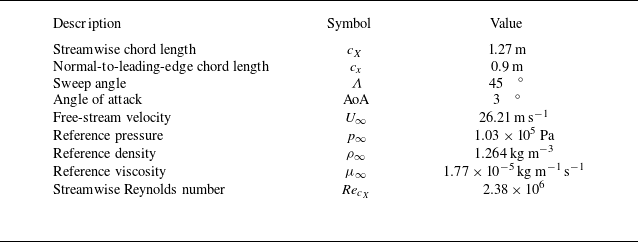


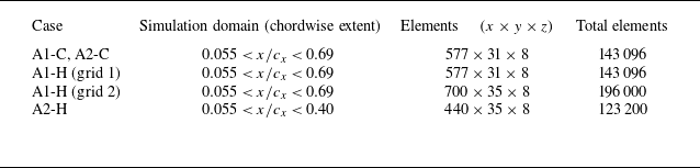


 Open access