


1. Introduction
The structure of the transition layer between unmagnetised plasma and a vacuum magnetic field has been actively discussed for approximately a century. Apparently, the interest in this problem first arose with regard to the phenomenon of plasma flow around the Earth’s magnetosphere and the formation of a relatively narrow transition layer (magnetopause), in which the decrease in plasma density and pressure was balanced by the increase in magnetic field pressure (Chapman & Ferraro Reference Chapman and Ferraro1931; Ferraro Reference Ferraro1952). Then the problem of plasma confinement with the maximum possible pressure in a magnetic field became relevant for $\theta$
-pinches (Rosenbluth Reference Rosenbluth1957). The first kinetic solutions describing the equilibrium of a plasma with the relative pressure
$\theta$
-pinches (Rosenbluth Reference Rosenbluth1957). The first kinetic solutions describing the equilibrium of a plasma with the relative pressure $\beta = 1$
were constructed by Grad (Reference Grad1961). His theory assumed a flat boundary and completely neglected the electric field of charge separation, which is valid either for equal particle masses
$\beta = 1$
were constructed by Grad (Reference Grad1961). His theory assumed a flat boundary and completely neglected the electric field of charge separation, which is valid either for equal particle masses $m_i = m_e$
(electron–positron plasma) or for a special relationship between the temperatures of the electron and ion components (
$m_i = m_e$
(electron–positron plasma) or for a special relationship between the temperatures of the electron and ion components ( $T_i / T_e = m_e / m_i$
). A more general theory, which took into account the possibility of a finite jump in the electric potential in a flat transition layer, was formulated by Schmidt & Finkelstein (Reference Schmidt and Finkelstein1962). But even the first numerical solutions of the complete system of equations (Paskievici Reference Paskievici1962) revealed a challenge: if there are no trapped electrons in the transition layer, the quasi-neutrality condition cannot be satisfied and the electric field grows without limit with radius, leading to unlimited acceleration of the ions. The first examples of an axially symmetric equilibrium with extremely high beta were proposed in the models (Harris Reference Harris1962; Komarov & Fadeev Reference Komarov and Fadeev1962; Nicholson Reference Nicholson1963), where the particle distribution functions
$T_i / T_e = m_e / m_i$
). A more general theory, which took into account the possibility of a finite jump in the electric potential in a flat transition layer, was formulated by Schmidt & Finkelstein (Reference Schmidt and Finkelstein1962). But even the first numerical solutions of the complete system of equations (Paskievici Reference Paskievici1962) revealed a challenge: if there are no trapped electrons in the transition layer, the quasi-neutrality condition cannot be satisfied and the electric field grows without limit with radius, leading to unlimited acceleration of the ions. The first examples of an axially symmetric equilibrium with extremely high beta were proposed in the models (Harris Reference Harris1962; Komarov & Fadeev Reference Komarov and Fadeev1962; Nicholson Reference Nicholson1963), where the particle distribution functions $f \propto \exp (\mathcal{E} - F(\mathcal{P}_\theta ))$
, depending only on the integrals of motion (energy
$f \propto \exp (\mathcal{E} - F(\mathcal{P}_\theta ))$
, depending only on the integrals of motion (energy $\mathcal{E}$
and azimuthal generalized momentum
$\mathcal{E}$
and azimuthal generalized momentum $\mathcal{P}_{\theta}$
), corresponded either to the rotation of a various plasma components
$\mathcal{P}_{\theta}$
), corresponded either to the rotation of a various plasma components $F \propto \mathcal{P}_\theta$
, or to the non-gyrotropy of their pressures
$F \propto \mathcal{P}_\theta$
, or to the non-gyrotropy of their pressures $F \propto \mathcal{P}_\theta ^2$
. However, in construction of specific solutions these models were also limited to the case of zero electric field.
$F \propto \mathcal{P}_\theta ^2$
. However, in construction of specific solutions these models were also limited to the case of zero electric field.
Currently, the structure of the transition layer in equilibria with $\beta \sim 1$
has again become the subject of active research for two reasons. Firstly, sub-ion magnetic holes were discovered in cosmic plasma having a characteristic size of the magnetic field change smaller than the ion gyroradius
$\beta \sim 1$
has again become the subject of active research for two reasons. Firstly, sub-ion magnetic holes were discovered in cosmic plasma having a characteristic size of the magnetic field change smaller than the ion gyroradius $\rho _i$
(Goodrich et al. Reference Goodrich2016; Huang et al. Reference Huang2019). It turned out that the stationary solutions of the Vlasov kinetic equation utilised in previous works (Harris Reference Harris1962; Komarov & Fadeev Reference Komarov and Fadeev1962; Nicholson Reference Nicholson1963) can be useful in explaining the structure of these magnetic holes, if the problem with quasi-neutrality violation in the cylindrical transition layer is solved by adding a background plasma (Shustov et al. Reference Shustov, Artemyev, Vasko and Yushkov2016). It was shown that the theory accounting for the electron kinetics allows a situation where the magnetic field gradient in these holes is characterised by two different scales – the electron and ion gyroradii (
$\rho _i$
(Goodrich et al. Reference Goodrich2016; Huang et al. Reference Huang2019). It turned out that the stationary solutions of the Vlasov kinetic equation utilised in previous works (Harris Reference Harris1962; Komarov & Fadeev Reference Komarov and Fadeev1962; Nicholson Reference Nicholson1963) can be useful in explaining the structure of these magnetic holes, if the problem with quasi-neutrality violation in the cylindrical transition layer is solved by adding a background plasma (Shustov et al. Reference Shustov, Artemyev, Vasko and Yushkov2016). It was shown that the theory accounting for the electron kinetics allows a situation where the magnetic field gradient in these holes is characterised by two different scales – the electron and ion gyroradii ( $\rho _e$
and
$\rho _e$
and $\rho _i$
). Later, such a two-scale structure of magnetic holes was confirmed by the observations of Li et al. Reference Li(2020). Secondly, today, high-beta equilibria seem promising for an implementation of improved diamagnetic plasma confinement in mirror traps (Beklemishev Reference Beklemishev2016) and for the creation of a fusion reactor prototype on their basis (GDMT project (Skovorodin et al. Reference Skovorodin2023)). As has been shown, the creation of a diamagnetic bubble with the large radius
$\rho _i$
). Later, such a two-scale structure of magnetic holes was confirmed by the observations of Li et al. Reference Li(2020). Secondly, today, high-beta equilibria seem promising for an implementation of improved diamagnetic plasma confinement in mirror traps (Beklemishev Reference Beklemishev2016) and for the creation of a fusion reactor prototype on their basis (GDMT project (Skovorodin et al. Reference Skovorodin2023)). As has been shown, the creation of a diamagnetic bubble with the large radius $a$
and thin transition layer with the width
$a$
and thin transition layer with the width $\lambda$
(
$\lambda$
( $\lambda \ll a$
), where the magnetic field increases from zero to the vacuum value, should reduce the longitudinal plasma losses in a mirror trap by a factor of
$\lambda \ll a$
), where the magnetic field increases from zero to the vacuum value, should reduce the longitudinal plasma losses in a mirror trap by a factor of $a / \lambda$
(Chernoshtanov Reference Chernoshtanov2022). To determine the width of the transition layer in a diamagnetic bubble, a theory was proposed by Kotelnikov (Reference Kotelnikov2020) in which the following distribution function was used as a stationary solution of the Vlasov kinetic equation for ions:
$a / \lambda$
(Chernoshtanov Reference Chernoshtanov2022). To determine the width of the transition layer in a diamagnetic bubble, a theory was proposed by Kotelnikov (Reference Kotelnikov2020) in which the following distribution function was used as a stationary solution of the Vlasov kinetic equation for ions:
 \begin{equation} f_i(\boldsymbol{r}, \boldsymbol{v})\propto e^{-\mathcal{E} / T} \mathcal{H}\left (\mathcal{P}_\theta ^{\mathrm{max}} - \mathcal{P}_\theta \right )\!, \end{equation}
where $\mathcal{E} = mv^2/2$
is the ion energy,
$\mathcal{E} = mv^2/2$
is the ion energy, $\mathcal{P}_\theta (\boldsymbol{r}, {\boldsymbol{v}})$
is ions generalised azimuthal momentum,
$\mathcal{P}_\theta (\boldsymbol{r}, {\boldsymbol{v}})$
is ions generalised azimuthal momentum, $\boldsymbol{v}$
is the velocity and
$\boldsymbol{v}$
is the velocity and $\mathcal{H}$
is the Heaviside function (equal 1 for positive arguments and 0 for negative arguments). In contrast to the axially symmetric distributions used in Komarov & Fadeev (Reference Komarov and Fadeev1962) and Nicholson (Reference Nicholson1963), this distribution allows the existence of a finite-radius core in the plasma column, wherein the particle density and pressure do not depend on coordinates, and the current is completely absent. Neglecting the finite temperature of the electrons and the electric field related to it, this theory predicted that the diamagnetic ion current should be localised to a size of approximately
$\mathcal{H}$
is the Heaviside function (equal 1 for positive arguments and 0 for negative arguments). In contrast to the axially symmetric distributions used in Komarov & Fadeev (Reference Komarov and Fadeev1962) and Nicholson (Reference Nicholson1963), this distribution allows the existence of a finite-radius core in the plasma column, wherein the particle density and pressure do not depend on coordinates, and the current is completely absent. Neglecting the finite temperature of the electrons and the electric field related to it, this theory predicted that the diamagnetic ion current should be localised to a size of approximately $10 \, \rho _i$
, where the ion Larmor radius is measured by the vacuum magnetic field. Subsequent Particle-In-Cell (PIC) studies (Kurshakov & Timofeev Reference Kurshakov and Timofeev2023; Timofeev, Kurshakov & Berendeev Reference Timofeev, Kurshakov and Berendeev2024) showed that the obtained equilibrium is unstable with respect to ion-cyclotron drift perturbations that initiate transition to another equilibrium, in which an electric field arises, leading to the dominance of the electron current in the internal part of the transition layer. In this case, the current was found to localise at an electron scale
$10 \, \rho _i$
, where the ion Larmor radius is measured by the vacuum magnetic field. Subsequent Particle-In-Cell (PIC) studies (Kurshakov & Timofeev Reference Kurshakov and Timofeev2023; Timofeev, Kurshakov & Berendeev Reference Timofeev, Kurshakov and Berendeev2024) showed that the obtained equilibrium is unstable with respect to ion-cyclotron drift perturbations that initiate transition to another equilibrium, in which an electric field arises, leading to the dominance of the electron current in the internal part of the transition layer. In this case, the current was found to localise at an electron scale $30 \, \rho _e$
(Timofeev et al. Reference Timofeev, Kurshakov and Berendeev2024). A similar conclusion about the formation of an even smaller-scale current sheet (
$30 \, \rho _e$
(Timofeev et al. Reference Timofeev, Kurshakov and Berendeev2024). A similar conclusion about the formation of an even smaller-scale current sheet ( ${\sim} 4 \, \rho _e$
) was made by Park et al. (Reference Park, Lapenta, Gonzalez-Herrero and Krall2019), where the plasma confinement in a multicusp trap was simulated.
${\sim} 4 \, \rho _e$
) was made by Park et al. (Reference Park, Lapenta, Gonzalez-Herrero and Krall2019), where the plasma confinement in a multicusp trap was simulated.
The reason for such a strong difference in the estimates of the layer width between theory ( $10 \, \rho _i$
) and simulations (
$10 \, \rho _i$
) and simulations ( $(4 {-} 30) \, \rho _e$
) is that the theory does not account for electron currents at all, while the numerical models apparently increase the role of a radial electric field capable of creating an uncompensated
$(4 {-} 30) \, \rho _e$
) is that the theory does not account for electron currents at all, while the numerical models apparently increase the role of a radial electric field capable of creating an uncompensated $\boldsymbol{E}\times \boldsymbol{B}$
-drift (electric and magnetic fields) of electrons at sub-ion scales. Indeed, all the mentioned PIC simulations were performed using periodic boundary conditions along the vacuum magnetic field, which requires conservation of the total charge of the system. In the absence of secondary electron emission from plasma receivers, simulations cannot produce the additional electrons naturally arising in real experiments. These electrons could travel from the walls along the magnetic field lines and compensate for the charge separation arising from the large difference in the Larmor radii of particles. Thus, the purpose of this work is to generalise the Kotelnikov theory to the case of finite electron temperature. We also aim at answering the question about the influence of electron currents on the size and structure of the transition layer, assuming that cold electrons can freely compensate for the lack of hot electrons at the plasma edge.
$\boldsymbol{E}\times \boldsymbol{B}$
-drift (electric and magnetic fields) of electrons at sub-ion scales. Indeed, all the mentioned PIC simulations were performed using periodic boundary conditions along the vacuum magnetic field, which requires conservation of the total charge of the system. In the absence of secondary electron emission from plasma receivers, simulations cannot produce the additional electrons naturally arising in real experiments. These electrons could travel from the walls along the magnetic field lines and compensate for the charge separation arising from the large difference in the Larmor radii of particles. Thus, the purpose of this work is to generalise the Kotelnikov theory to the case of finite electron temperature. We also aim at answering the question about the influence of electron currents on the size and structure of the transition layer, assuming that cold electrons can freely compensate for the lack of hot electrons at the plasma edge.
2. Revision of Kotelnikov's theory for cold electrons
Before examining the effects of finite electron temperature, we reformulate Kotelnikov’s theory for cold electrons so that it solves the problem of Grad (Reference Grad1961) for the minimal-size transition layer in which trapped ions are absent. The subsequent analysis shows that the distribution (2.3) corresponds to a specific loading of the transition layer by trapped particles. In the cold electron approximation, we can completely neglect the electric field and consider the motion of ions only under the action of the Lorentz force. As in the original paper (Kotelnikov Reference Kotelnikov2020), we will assume that an isotropic Maxwellian plasma with a uniform density $n_0$
and temperature
$n_0$
and temperature $T$
is created inside a certain radius
$T$
is created inside a certain radius $a$
. The magnetic field is directed along the plasma column axis and it is uniform for
$a$
. The magnetic field is directed along the plasma column axis and it is uniform for $r \lt a$
:
$r \lt a$
: $B_z(r) = B_{\mathrm{in}}$
. The transition layer lies in the region
$B_z(r) = B_{\mathrm{in}}$
. The transition layer lies in the region $r \gt a$
, where the plasma density and pressure gradually decrease, and the magnetic field increases to the value of the vacuum field
$r \gt a$
, where the plasma density and pressure gradually decrease, and the magnetic field increases to the value of the vacuum field $B_z(\infty ) = B_v$
. The problem of Grad suggests that all particles in the layer are passing ones, that is, they all come from the region
$B_z(\infty ) = B_v$
. The problem of Grad suggests that all particles in the layer are passing ones, that is, they all come from the region $r \lt a$
. Moving in a transversely inhomogeneous and axially symmetric magnetic field
$r \lt a$
. Moving in a transversely inhomogeneous and axially symmetric magnetic field $B_z = \chi ^{\prime }(r) / r$
, particles must conserve energy
$B_z = \chi ^{\prime }(r) / r$
, particles must conserve energy $\mathcal{E} = mv_{\bot }^2 / 2$
and the azimuthal generalised momentum
$\mathcal{E} = mv_{\bot }^2 / 2$
and the azimuthal generalised momentum $\mathcal{P}_\theta = mv_{\bot }r \sin (\theta - \varphi ) + e\chi (r) / c$
, where
$\mathcal{P}_\theta = mv_{\bot }r \sin (\theta - \varphi ) + e\chi (r) / c$
, where
 \begin{align*} \boldsymbol{v}_{\bot } = (v_{\bot }\cos \theta , v_{\bot }\sin \theta ), \qquad \boldsymbol{r} = (r\cos \varphi , r\sin \varphi ), \end{align*}
and $\chi (r)$
is a quantity proportional to the magnetic flux
$\chi (r)$
is a quantity proportional to the magnetic flux
 \begin{equation} \chi (r)=\int \limits _0^r B_z(r^{\prime }) r^{\prime }\,\text{d}r^{\prime }. \end{equation}
We can use any function of the integrals of motion $\mathcal{E}$
and
$\mathcal{E}$
and $\mathcal{P}_\theta$
to describe the stationary particle distribution in a transition layer. The only restriction is that it should be matched with the isotropic Maxwellian function at
$\mathcal{P}_\theta$
to describe the stationary particle distribution in a transition layer. The only restriction is that it should be matched with the isotropic Maxwellian function at $r = a$
. In Kotelnikov (Reference Kotelnikov2020), it was proposed to use the function
$r = a$
. In Kotelnikov (Reference Kotelnikov2020), it was proposed to use the function
 \begin{equation} f_i(\boldsymbol{r},\boldsymbol{v}_{\bot })=\frac {n_0}{2\pi v_T^2}e^{-\mathcal{E}/T} \mathcal{H}\left (\mathcal{P}_\theta ^{\mathrm{max}}-\mathcal{P}_\theta \right )\!, \end{equation}
which limits the range of possible values of the azimuthal momentum for each selected $v_{\bot }$
by
$v_{\bot }$
by $\mathcal{P}_\theta ^{\mathrm{max}} = mv_{\bot }a + e\chi (a) / c$
(
$\mathcal{P}_\theta ^{\mathrm{max}} = mv_{\bot }a + e\chi (a) / c$
( $\mathcal{H}$
is the Heaviside function,
$\mathcal{H}$
is the Heaviside function, $v_T = \sqrt {T / m}$
is the thermal velocity). However, in a cylindrical plasma with radius
$v_T = \sqrt {T / m}$
is the thermal velocity). However, in a cylindrical plasma with radius $a$
, the azimuthal momentum is limited not only from above but also from below. Indeed, when the magnetic field is completely expelled from the plasma (
$a$
, the azimuthal momentum is limited not only from above but also from below. Indeed, when the magnetic field is completely expelled from the plasma ( $B_{\mathrm{in}} = 0$
,
$B_{\mathrm{in}} = 0$
, $\chi (r \lt a) = 0$
), the azimuthal momentum cannot be less than a value
$\chi (r \lt a) = 0$
), the azimuthal momentum cannot be less than a value $\mathcal{P}_\theta ^{\mathrm{min}} = -mv_{\bot }a$
. For finite
$\mathcal{P}_\theta ^{\mathrm{min}} = -mv_{\bot }a$
. For finite $B_{\mathrm{in}}$
, the function
$B_{\mathrm{in}}$
, the function $\chi (r)$
inside a homogeneous plasma grows according to the parabolic law
$\chi (r)$
inside a homogeneous plasma grows according to the parabolic law $\chi = B_{\mathrm{in}}r^2 / 2$
, therefore the minimum value of the azimuthal momentum corresponding to the minimum possible azimuthal velocity
$\chi = B_{\mathrm{in}}r^2 / 2$
, therefore the minimum value of the azimuthal momentum corresponding to the minimum possible azimuthal velocity $-v_{\bot }$
depends non-monotonically on the radius:
$-v_{\bot }$
depends non-monotonically on the radius: $\mathcal{P}_\theta ^{\mathrm{min}} = -mv_{\bot }r + e\chi (r) / c$
. For
$\mathcal{P}_\theta ^{\mathrm{min}} = -mv_{\bot }r + e\chi (r) / c$
. For $r \lt b = v_{\bot } / (eB_{\mathrm{in}} / mc)$
the lower threshold of the azimuthal momentum
$r \lt b = v_{\bot } / (eB_{\mathrm{in}} / mc)$
the lower threshold of the azimuthal momentum $\mathcal{P}_\theta ^{\mathrm{min}}(r)$
decreases with the increase in radius, therefore in case
$\mathcal{P}_\theta ^{\mathrm{min}}(r)$
decreases with the increase in radius, therefore in case $a \lt b$
, as before, the global minimum is reached at the largest radius
$a \lt b$
, as before, the global minimum is reached at the largest radius $a$
of the isotropic section of plasma. If
$a$
of the isotropic section of plasma. If $a \gt b$
, then
$a \gt b$
, then $\mathcal{P}_\theta ^{\mathrm{ min}}(r)$
increases with
$\mathcal{P}_\theta ^{\mathrm{ min}}(r)$
increases with $r$
, and the global minimum of this function is achieved inside the isotropic plasma, at the radius
$r$
, and the global minimum of this function is achieved inside the isotropic plasma, at the radius $b$
. Thus, the lower limit on the magnitude of the azimuthal generalised momentum depends on the ratio between the plasma radius
$b$
. Thus, the lower limit on the magnitude of the azimuthal generalised momentum depends on the ratio between the plasma radius $a$
and the Larmor radius of ion
$a$
and the Larmor radius of ion $b$
, calculated from the internal magnetic field
$b$
, calculated from the internal magnetic field $B_{\mathrm{ in}}$
 \begin{equation} \mathcal{P}_\theta ^{\mathrm{min}} = \begin{cases} -mv_{\bot }a + e\chi (a) / c, & a \lt b, \\ -mv_{\bot }b + e\chi (b) / c, & a \gt b. \end{cases} \end{equation}
(a) Blue stripes are the ranges of possible values of the azimuthal generalised momentum $\mathcal{P}_{\theta }=mv_{\bot }r\sin \theta +e\chi (r)/c$
at different radii for ions with two chosen values of
$\mathcal{P}_{\theta }=mv_{\bot }r\sin \theta +e\chi (r)/c$
at different radii for ions with two chosen values of $v_{\bot }$
, if the particles had an isotropic angular distribution everywhere (for
$v_{\bot }$
, if the particles had an isotropic angular distribution everywhere (for $\chi (r)$
, the self-consistent solution at
$\chi (r)$
, the self-consistent solution at $a=10$
and
$a=10$
and $B_{\mathrm{in}}=0.01$
is used). Green and orange lines are the constraints
$B_{\mathrm{in}}=0.01$
is used). Green and orange lines are the constraints $\mathcal{P}_\theta ^{\mathrm{max}}(a)$
and
$\mathcal{P}_\theta ^{\mathrm{max}}(a)$
and $\mathcal{P}_\theta ^{\mathrm{min}}(a)$
, which allow ions to have an isotropic distribution only in the region
$\mathcal{P}_\theta ^{\mathrm{min}}(a)$
, which allow ions to have an isotropic distribution only in the region $r\lt a$
and separate passing particles from trapped ones in the transition layer. The regions of trapped particles that are not cut off in the Kotelnikov distribution are shaded in red (2.3). (b) Particle trajectories corresponding to the square and round dots in (a); the blue solid trajectory touches the core of the diamagnetic bubble and corresponds to particles at the boundary between the passing and trapped zones, while the orange dotted trajectory belongs to a particle trapped in the transition layer and lies entirely outside the isotropic core.
$r\lt a$
and separate passing particles from trapped ones in the transition layer. The regions of trapped particles that are not cut off in the Kotelnikov distribution are shaded in red (2.3). (b) Particle trajectories corresponding to the square and round dots in (a); the blue solid trajectory touches the core of the diamagnetic bubble and corresponds to particles at the boundary between the passing and trapped zones, while the orange dotted trajectory belongs to a particle trapped in the transition layer and lies entirely outside the isotropic core.

Given this additional constraint, the ion distribution function describing only passing particles in the transition layer must differ from the distribution function (2.3) as follows:
 \begin{equation} f_i(\boldsymbol{r}, \boldsymbol{v}_{\bot }) = \frac {n_0}{2\pi v_T^2} \exp \left ( \frac {v_{\bot }^2}{2v_T^2} \right ) \left [ \mathcal{H} \left (\mathcal{P}_\theta ^{\mathrm{max}} - \mathcal{P}_\theta \right ) - \mathcal{H} \left (\mathcal{P}_\theta ^{\mathrm{min}} - \mathcal{P}_\theta \right ) \right ]\!. \end{equation}
To illustrate the differences between the two distribution functions, we show figure 1. If the particles at all radii had an isotropic angular distribution, then the possible values of the azimuthal generalised momentum for two chosen $v_{\bot }$
would lie inside the ranges shown in figure 1(a) by the light blue and dark blue stripes. The constraints
$v_{\bot }$
would lie inside the ranges shown in figure 1(a) by the light blue and dark blue stripes. The constraints $\mathcal{P}_\theta ^{\mathrm{max}}$
and
$\mathcal{P}_\theta ^{\mathrm{max}}$
and $\mathcal{P}_\theta ^{\mathrm{min}}$
(green and orange straight lines) leave the ion angular distribution isotropic only inside the region
$\mathcal{P}_\theta ^{\mathrm{min}}$
(green and orange straight lines) leave the ion angular distribution isotropic only inside the region $r\lt a$
and separate the passing particles from those trapped in the transition layer
$r\lt a$
and separate the passing particles from those trapped in the transition layer $r\gt a$
. Kotelnikov’s distribution (2.3) cuts off trapped particles only with large positive values of
$r\gt a$
. Kotelnikov’s distribution (2.3) cuts off trapped particles only with large positive values of $\mathcal{P}_\theta$
and leaves trapped particles in the transition layer, which fill the red regions in figure 1(a). Figure 1(b) shows that the particles with
$\mathcal{P}_\theta$
and leaves trapped particles in the transition layer, which fill the red regions in figure 1(a). Figure 1(b) shows that the particles with $\mathcal{P}_\theta \lt \mathcal{P}^{\mathrm{min}}_\theta$
present in the model of Kotelnikov indeed never enter the isotropic core of the diamagnetic bubble, and their trajectories lie entirely in the region
$\mathcal{P}_\theta \lt \mathcal{P}^{\mathrm{min}}_\theta$
present in the model of Kotelnikov indeed never enter the isotropic core of the diamagnetic bubble, and their trajectories lie entirely in the region $r\gt a$
. It is obvious that the population of particles trapped in the transition layer disappears if the plasma size
$r\gt a$
. It is obvious that the population of particles trapped in the transition layer disappears if the plasma size $a$
exceeds the ion gyroradius
$a$
exceeds the ion gyroradius $b$
in the field
$b$
in the field $B_{\mathrm{in}}$
.
$B_{\mathrm{in}}$
.
Constraints on azimuthal momentum for each value of $v_{\bot }$
can be formulated as a restrictions on possible velocity vector directions (angle
$v_{\bot }$
can be formulated as a restrictions on possible velocity vector directions (angle $\theta$
)
$\theta$
)
 \begin{equation} \xi _{\mathrm{min}}\lt \sin (\theta -\varphi )\lt \xi _{\mathrm{max}}, \end{equation}
where
 \begin{equation} \xi _{\mathrm{max}} = \frac {a - \bar {\chi } / v_{\bot }}{r},\qquad\qquad\qquad\quad \end{equation}
 \begin{align}\qquad\quad\qquad \xi_{\mathrm{min}} & = \left\{\begin{array}{l@{\quad}l} -\left [a + \bar {\chi } / v_{\bot }\right ] / r, & v_{\bot } \gt aB_{\mathrm{in}},\\[5pt] -\left [b + (\bar {\chi } + \varDelta \chi ) / v_{\bot }\right ] / r, & v_{\bot } \lt aB_{\mathrm{in}}, \end{array}\right.\end{align}
 \begin{equation} \bar {\chi } = \chi (r) - \chi (a), \qquad \varDelta \chi = \chi (a) - \chi (b). \end{equation}
The quantities above are in the dimensionless form, velocities are measured in units of the light speed $c$
, spatial scales are in units of
$c$
, spatial scales are in units of $c / \omega _{pi}$
,
$c / \omega _{pi}$
, $\omega_{pi}=\sqrt(4\pi e^2 n_0/m_i)$
is the ion plasma frequency and magnetic field is in units of
$\omega_{pi}=\sqrt(4\pi e^2 n_0/m_i)$
is the ion plasma frequency and magnetic field is in units of $mc\omega _{pi} / e$
. Clearly, in the region accessible to particle motion, the interval
$mc\omega _{pi} / e$
. Clearly, in the region accessible to particle motion, the interval $[\xi _{\mathrm{min}}, \xi _{\mathrm{max}}]$
should overlap with
$[\xi _{\mathrm{min}}, \xi _{\mathrm{max}}]$
should overlap with $[-1, 1]$
.
$[-1, 1]$
.
The density distribution in the transition layer can be found by calculating the integral
 \begin{equation} n(r) = \int \limits _0^{\infty } {\rm d}v_{\bot } v_{\bot } \int \limits _{-\pi }^{\pi } {\rm d}\theta f_i. \end{equation}
Substitution of distribution function (2.5) into this integral gives
 \begin{align} n(r) &= \frac {1}{\pi v_T^2} \int \limits _0^{\infty } {\rm d}v_{\bot } v_{\bot } \exp \left (-\frac {v_{\bot }^2}{2v_T^2}\right ) \nonumber \\ &\quad \times \begin{cases} \arcsin \xi _{\mathrm{max}} - \arcsin \xi _{\mathrm{min}}, & v_{\bot } \gt V, \\ \pi /2 + \arcsin \xi _{\mathrm{max}}, & \bar {\chi } / (r + a) \lt v_{\bot } \lt V, \\ 0, & v_{\bot } \lt \bar {\chi } / (r + a). \end{cases} \end{align}
Here, the speed $V$
depends on the magnitude of the magnetic field in the centre of the plasma
$V$
depends on the magnitude of the magnetic field in the centre of the plasma
 \begin{equation} V = \begin{cases} \bar {\chi } / (r - a), & \bar {\chi } / (r - a) \gt aB_{\mathrm{in}}, \\ B_{\mathrm{in}} \left (r - \sqrt {r^2 - 2\chi (r) / B_{\mathrm{in}}}\right )\!, & \bar {\chi } / (r - a) \lt aB_{\mathrm{in}}. \end{cases} \end{equation}
The azimuthal current density distribution can be calculated likewise
 \begin{equation} J_\varphi (r) = e\int \limits _0^{\infty } {\rm d}v_{\bot } v_{\bot } \int \limits _{-\pi }^{\pi } {\rm d}\theta v_{\bot }\sin (\theta - \varphi ) f_i. \end{equation}
In units of $en_0c$
it can be represented as
$en_0c$
it can be represented as
 \begin{align} J_\varphi &= \frac {1}{\pi v_T^2} \int \limits _0^{\infty } {\rm d}v_{\bot } v_{\bot }^2 \exp \left (-\frac {v_{\bot }^2}{2v_T^2}\right ) \nonumber \\&\quad \times \begin{cases} \sqrt {1 - \xi _{\mathrm{min}}^2}-\sqrt {1 - \xi _{\mathrm{max}}^2}, & v_{\bot } \gt V, \\[5pt] -\sqrt {1 - \xi _{\mathrm{max}}^2}, & \bar {\chi } / (r + a) \lt v_{\bot } \lt V, \\[5pt] 0, & v_{\bot } \lt \bar {\chi } / (r + a). \end{cases} \end{align}
Radial equilibrium of axisymmetric plasma depends on two components of the momentum flux tensor
 \begin{equation}\varPi _{rr} = \int \limits _0^{\infty } \text{d}v_{\bot } v_{\bot } \int \limits _{-\pi }^{\pi } \text{d}\theta mv_{\bot }^2 \cos ^2(\theta - \varphi ) f_i, \end{equation}
 \begin{equation} \varPi _{\varphi \varphi } = \int \limits _0^{\infty } \text{d}v_{\bot } v_{\bot } \int \limits _{-\pi }^{\pi } \text{d}\theta mv_{\bot }^2 \sin ^2(\theta - \varphi ) f_i. \end{equation}
Represented in units of $n_0mc^2$
it can be written as
$n_0mc^2$
it can be written as
 \begin{equation} \varPi _{rr,\varphi \varphi } = \frac {1}{2\pi v_T^2} \int \limits _0^{\infty } \text{d}v_{\bot } v_{\bot }^3 \exp \left (-\frac {v_{\bot }^2}{2v_T^2}\right ) \begin{cases} \varPi _1, & v_{\bot } \gt V, \\ \varPi _2, & \bar {\chi } / (r + a) \lt v_{\bot } \lt V, \\ 0, & v_{\bot } \lt \bar {\chi } / (r + a), \end{cases} \end{equation}
where
 \begin{align} \varPi _1 = \arcsin \xi _{\mathrm{max}} - \arcsin \xi _{\mathrm{min}} \pm \left (\xi _{\mathrm{max}}\sqrt {1 - \xi _{\mathrm{max}}^2} - \xi _{\mathrm{min}}\sqrt {1 - \xi _{\mathrm{min}}^2}\right )\!, \end{align}
 \begin{align} \varPi _2 = \arcsin \xi _{\mathrm{max}} + \frac {\pi }{2} \pm \xi _{\mathrm{max}}\sqrt {1 - \xi _{\mathrm{max}}^2} \end{align}
(top sign for $\varPi _{rr}$
, bottom sign for
$\varPi _{rr}$
, bottom sign for $\varPi _{\varphi \varphi }$
). It can be seen that quantities of
$\varPi _{\varphi \varphi }$
). It can be seen that quantities of $\varPi _{rr}$
,
$\varPi _{rr}$
, $\varPi _{\varphi \varphi }$
and
$\varPi _{\varphi \varphi }$
and $J_\varphi$
calculated this way do satisfy the radial equilibrium equation
$J_\varphi$
calculated this way do satisfy the radial equilibrium equation
 \begin{equation} -\frac {\partial \varPi _{rr}}{\partial r} - \frac {\varPi _{rr} - \varPi _{\varphi \varphi }}{r} + J_\varphi B_z = 0. \end{equation}
Comparison of the Kotelnikov (Reference Kotelnikov2020) theory (a, c, e, g) and its modified version (b, d, f, h) at $B_{\mathrm{ in}}=0.1$
(
$B_{\mathrm{ in}}=0.1$
( $T_i = 10$
keV,
$T_i = 10$
keV, $T_e = 0$
): equilibrium profiles of the plasma density, azimuthal current density and magnetic field at
$T_e = 0$
): equilibrium profiles of the plasma density, azimuthal current density and magnetic field at $a = 10$
(a, b) and at
$a = 10$
(a, b) and at $a = 1.5$
(e, f); profiles of
$a = 1.5$
(e, f); profiles of $\varPi _{rr}$
,
$\varPi _{rr}$
, $\varPi _{\varphi \varphi }$
,
$\varPi _{\varphi \varphi }$
, $\varDelta \varPi$
and
$\varDelta \varPi$
and $B^2 / 2$
at
$B^2 / 2$
at $a = 10$
(c, d) and at
$a = 10$
(c, d) and at $a = 1.5$
(g, h).
$a = 1.5$
(g, h).

Substituting the current created by the ions into the Maxwell’s equation $-B_z^{\prime } = J_\varphi$
, we obtain an ordinary differential equation for determining the magnetic flux profile
$-B_z^{\prime } = J_\varphi$
, we obtain an ordinary differential equation for determining the magnetic flux profile $\bar {\chi }(r)$
in the transition layer
$\bar {\chi }(r)$
in the transition layer
 \begin{equation} \frac {\text{d}}{\text{d}r}\left (\frac {1}{r}\frac {\text{d} \bar {\chi }}{\text{d}r}\right ) = -J_\varphi , \end{equation}
that should be solved with the boundary conditions: $\bar {\chi }(a) = 0$
,
$\bar {\chi }(a) = 0$
, $\bar {\chi }^{\prime }(a) = aB_{\mathrm{in}}$
.
$\bar {\chi }^{\prime }(a) = aB_{\mathrm{in}}$
.
Comparison of the Kotelnikov (Reference Kotelnikov2020) theory (a, c) and its modified version (b, d) with almost complete displacement of the magnetic field $B_{\mathrm{in}} = 0.01$
(
$B_{\mathrm{in}} = 0.01$
( $T_i = 10$
keV,
$T_i = 10$
keV, $T_e = 0$
): equilibrium profiles of plasma density, azimuthal current density and magnetic field (a, b) and the corresponding pressure balance (c, d).
$T_e = 0$
): equilibrium profiles of plasma density, azimuthal current density and magnetic field (a, b) and the corresponding pressure balance (c, d).

Figure 2 shows how strongly the additional constraint on the azimuthal momentum we have introduced affects the equilibrium profiles of the plasma and magnetic field. The graphs in figures 2(a), 2(c), 2(e) and 2(g) were calculated using the Kotelnikov theory, in which the azimuthal generalised momentum is limited only from above, and figures 2(b), 2(d), 2(f) and 2(h) correspond to solutions of (2.21) with two constraints $\mathcal{P}^{\mathrm{min}}_\theta \lt \mathcal{P}_\theta \lt \mathcal{P}^{\mathrm{max}}_\theta$
. Let us first find the equilibrium in the case when a proton plasma with a temperature of
$\mathcal{P}^{\mathrm{min}}_\theta \lt \mathcal{P}_\theta \lt \mathcal{P}^{\mathrm{max}}_\theta$
. Let us first find the equilibrium in the case when a proton plasma with a temperature of $T=10$
keV and a sufficiently large radius of
$T=10$
keV and a sufficiently large radius of $a = 10$
reduces the magnetic field in its volume to a value of
$a = 10$
reduces the magnetic field in its volume to a value of $B_{\mathrm{in}} = 0.1$
(figures 2
a–d). It is evident from figures 2(a) and 2(b) that the differences between the two solutions in this regime are insignificant. The barely noticeable decrease in the vacuum magnetic field compared with Kotelnikov’s prediction is due to a slightly larger difference between the radial and azimuthal components of the momentum flux
$B_{\mathrm{in}} = 0.1$
(figures 2
a–d). It is evident from figures 2(a) and 2(b) that the differences between the two solutions in this regime are insignificant. The barely noticeable decrease in the vacuum magnetic field compared with Kotelnikov’s prediction is due to a slightly larger difference between the radial and azimuthal components of the momentum flux $\varPi _{rr}$
and
$\varPi _{rr}$
and $\varPi _{\varphi \varphi }$
, i.e. the stronger non-gyrotropy of the plasma. As discussed earlier (Kotelnikov Reference Kotelnikov2020; Timofeev et al. Reference Timofeev, Kurshakov and Berendeev2024), the non-gyrotropic effect results in the vacuum magnetic field pressure being less than the sum of the pressures inside the plasma
$\varPi _{\varphi \varphi }$
, i.e. the stronger non-gyrotropy of the plasma. As discussed earlier (Kotelnikov Reference Kotelnikov2020; Timofeev et al. Reference Timofeev, Kurshakov and Berendeev2024), the non-gyrotropic effect results in the vacuum magnetic field pressure being less than the sum of the pressures inside the plasma $\varPi _{rr}(0) + B_{\mathrm{in}}^2 / 2$
by
$\varPi _{rr}(0) + B_{\mathrm{in}}^2 / 2$
by
 \begin{equation} \varDelta \varPi = \int \limits _0^r \frac {\varPi _{rr} - \varPi _{\varphi \varphi }}{r^{\prime }} \text{d}r^{\prime }, \end{equation}
which follows directly from the integration of (2.20). To evaluate the role of the various components in this pressure balance, we show in figure 2(c, d, g, h) the profiles of $\varPi _{rr}$
and
$\varPi _{rr}$
and $B^2 / 2 + \varDelta \varPi$
. Their sum indeed remains constant at all radii
$B^2 / 2 + \varDelta \varPi$
. Their sum indeed remains constant at all radii
 \begin{equation} \varPi _{rr} + \frac {B^2}{2} + \varDelta \varPi = \varPi _{rr}(0) + \frac {B_{\mathrm{in}}^2}{2}. \end{equation}
A stronger difference between the two theories arises when a small plasma radius $a = 1.5$
, comparable to the Larmor radius of an ion in a vacuum field, is considered (figure 2
e–f). In this case, the modified theory predicts a wider transition layer and a several times lower vacuum magnetic field, which is associated with a much stronger plasma non-gyrotropy than it is in (Kotelnikov Reference Kotelnikov2020) (
$a = 1.5$
, comparable to the Larmor radius of an ion in a vacuum field, is considered (figure 2
e–f). In this case, the modified theory predicts a wider transition layer and a several times lower vacuum magnetic field, which is associated with a much stronger plasma non-gyrotropy than it is in (Kotelnikov Reference Kotelnikov2020) ( $\varDelta \varPi$
in figure 2(h) not only ceases to be a small addition, but becomes noticeably larger than
$\varDelta \varPi$
in figure 2(h) not only ceases to be a small addition, but becomes noticeably larger than $B^2 / 2$
). In other words, to be able to displace the magnetic field from a plasma of a sufficiently small radius, the plasma pressure must significantly exceed the pressure of the vacuum magnetic field. This conclusion may be important for the interpretation of experiments at the CAT facility (Bagryansky Reference Bagryansky2016), in which the plasma size is comparable to the gyroradius of fast ions arising due to neutral injection.
$B^2 / 2$
). In other words, to be able to displace the magnetic field from a plasma of a sufficiently small radius, the plasma pressure must significantly exceed the pressure of the vacuum magnetic field. This conclusion may be important for the interpretation of experiments at the CAT facility (Bagryansky Reference Bagryansky2016), in which the plasma size is comparable to the gyroradius of fast ions arising due to neutral injection.
A similar effect of increasing the non-gyrotropic addition and decreasing the vacuum magnetic field is also observed when the magnetic field $B_{\mathrm{in}}$
inside the isotropic plasma is decreased. Figure 3 shows that the almost complete displacement of the field (
$B_{\mathrm{in}}$
inside the isotropic plasma is decreased. Figure 3 shows that the almost complete displacement of the field ( $B_{\mathrm{in}} = 0.01$
) even at the large radius
$B_{\mathrm{in}} = 0.01$
) even at the large radius $a = 10$
leads to an increase in the contribution of
$a = 10$
leads to an increase in the contribution of $\varDelta \varPi$
and a decrease in the contribution of
$\varDelta \varPi$
and a decrease in the contribution of $B^2/2$
to the overall pressure balance.
$B^2/2$
to the overall pressure balance.
3. Accounting for the finite electron temperature
Let us now consider the case of a finite temperature of electrons. Let both ions and electrons have isotropic Maxwellian distributions inside the radius $a$
with the same densities and different temperatures
$a$
with the same densities and different temperatures $T_i$
and
$T_i$
and $T_e$
. Unlike the case of cold electrons, now the propagation of particles into the transition layer is affected not only by an increasing magnetic field
$T_e$
. Unlike the case of cold electrons, now the propagation of particles into the transition layer is affected not only by an increasing magnetic field $B_z(r)$
, but also a radial electric field
$B_z(r)$
, but also a radial electric field $E_r = -\partial \phi / \partial r$
. The latter occurs due to separation of charges produced by a large difference in the Larmor radii of electrons and ions. The ion distribution function in the transition layer (
$E_r = -\partial \phi / \partial r$
. The latter occurs due to separation of charges produced by a large difference in the Larmor radii of electrons and ions. The ion distribution function in the transition layer ( $r \gt a$
) has the same form as in (2.5) with the only difference that, instead of a velocity module, the value
$r \gt a$
) has the same form as in (2.5) with the only difference that, instead of a velocity module, the value $\mathcal{E} = mv_{\bot }^2(r) / 2 + e\phi (r)$
is now conserved. Taking into account the change in the particle velocity module at radius
$\mathcal{E} = mv_{\bot }^2(r) / 2 + e\phi (r)$
is now conserved. Taking into account the change in the particle velocity module at radius $r$
, compared with its value
$r$
, compared with its value $v_{\bot }$
in the isotropic section, the azimuthal generalised momentum is given by
$v_{\bot }$
in the isotropic section, the azimuthal generalised momentum is given by
 \begin{equation} \mathcal{P}_{\theta i} = m_i r \sqrt {v_{\bot }^2 - \frac {2e\phi (r)}{m_i}}\sin (\theta - \varphi ) + e\chi (r) / c. \end{equation}
Since $\phi = 0$
for
$\phi = 0$
for $r \lt a$
, the maximum and minimum values of this momentum (
$r \lt a$
, the maximum and minimum values of this momentum ( $\mathcal{P}_\theta ^{\mathrm{max}}$
and
$\mathcal{P}_\theta ^{\mathrm{max}}$
and $\mathcal{P}_\theta ^{\mathrm{min}}$
) remain unchanged. Then the restrictions on the possible values of
$\mathcal{P}_\theta ^{\mathrm{min}}$
) remain unchanged. Then the restrictions on the possible values of $\sin (\theta - \varphi )$
in the presence of an electric field in the layer are modified as follows:
$\sin (\theta - \varphi )$
in the presence of an electric field in the layer are modified as follows:
 \begin{equation} \xi _{\mathrm{i,max}} = \frac {a - \bar {\chi }/v_{\bot }}{r\sqrt {1 - \varPhi /v_{\bot }^2}},\qquad\qquad\quad \end{equation}
 \begin{equation} \;\qquad\qquad\xi _{\mathrm{i,min}} = \begin{cases} -\dfrac {a + \bar {\chi }/v_{\bot }}{r\sqrt {1 - \varPhi / v_{\bot }^2}}, & v_{\bot } \gt aB_{\mathrm{ in}}, \\[12pt] -\dfrac {b_i + (\bar {\chi } + \varDelta \chi ) / v_{\bot }}{r\sqrt {1 - \varPhi / v_{\bot }^2}}, & v_{\bot } \lt aB_{\mathrm{ in}}, \end{cases} \end{equation}
where $\varPhi = 2e\phi / (m_ic^2)$
is a dimensionless electric potential. Thus, the ion density and current density can be written as
$\varPhi = 2e\phi / (m_ic^2)$
is a dimensionless electric potential. Thus, the ion density and current density can be written as
 \begin{align} n_i(r) &= \frac {1}{\pi v_{Ti}^2} \int \limits _{\sqrt {\varPhi }}^{\infty } \text{d}v_{\bot } v_{\bot } \exp \left (-\frac {v_{\bot }^2}{2v_{Ti}^2}\right )\nonumber \\ &\quad \times \begin{cases} \arcsin \xi _{\mathrm{i,max}} - \arcsin \xi _{\mathrm{i,min}}, &|\xi _{\mathrm{i,max}}|, |\xi _{\mathrm{i,min}}| \lt 1 \\[6pt] \pi /2 + \arcsin \xi _{\mathrm{i,max}}, &|\xi _{\mathrm{i,max}}| \lt 1, \xi _{\mathrm{i,min}} \lt -1 \\[6pt] \pi /2 - \arcsin \xi _{\mathrm{i,min}}, &\xi _{\mathrm{i,max}} \gt 1, |\xi _{\mathrm{i,min}}| \lt 1 \\[6pt] 0, &|\xi _{\mathrm{i,max}}|, |\xi _{\mathrm{i,min}}| \gt 1, \end{cases} \end{align}
 \begin{align} J_{\varphi }^i &= \frac {1}{\pi v_{Ti}^2} \int \limits _{\sqrt {\varPhi }}^{\infty } \text{d}v_{\bot } v_{\bot }\sqrt {v_{\bot }^2 - \varPhi } \exp \left (-\frac {v_{\bot }^2}{2v_{Ti}^2}\right ) \nonumber \\[10pt] & \quad \times \left [\sqrt {1 - \xi _{\mathrm{i,min}}^2}\mathcal{H}(1 - \xi _{\mathrm{i,min}}^2) - \sqrt {1 - \xi _{\mathrm{ i,max}}^2}\mathcal{H}\big(1 - \xi _{\mathrm{i,max}}^2\big)\right ]\!. \end{align}
For electrons, the generalised azimuthal momentum can be obtained from the ion form by replacing the mass and sign of the electric charge
 \begin{equation} \mathcal{P}_{\theta e} = m_e r \sqrt {v_{\bot }^2 + \frac {2e\phi (r)}{m_e}}\sin (\theta -\varphi )-e\chi (r)/c. \end{equation}
Using the analogous definitions of the maximum and minimum values of this momentum inside an isotropic region of plasma, we obtain the following constraints on the electron velocity angles for $r \gt a$
:
$r \gt a$
:
 \begin{equation} \xi _{\mathrm{e,min}} \lt \sin (\theta -\varphi ) \lt \xi _{\mathrm{e,max}}, \end{equation}
where
 \begin{align} \xi _{\mathrm{e,min}} = -\frac {a - \mu \bar {\chi } / v_{\bot }}{r\sqrt {1 + \mu \varPhi / v_{\bot }^2}},\qquad\qquad \end{align}
 \begin{align}\qquad\qquad\; \xi _{\mathrm{e,max}} = \begin{cases} \dfrac {a + \mu \bar {\chi } / v_{\bot }}{r\sqrt {1 + \mu \varPhi / v_{\bot }^2}}, & v_{\bot } \gt a\mu B_{\mathrm{in}},\\[20pt] \dfrac {b_e + \mu (\bar {\chi } + \varDelta \chi ) / v_{\bot }}{r\sqrt {1 + \mu \varPhi / v_{\bot }^2}}, & v_{\bot } \lt a\mu B_{\mathrm{in}}, \end{cases} \end{align}
 \begin{eqnarray} b_e = v_{\bot } / (\mu B_{\mathrm{in}}), \qquad \mu = m_i / m_e. \end{eqnarray}
The density and current density of electrons is written by analogy with (3.4) and (3.5)
 \begin{align} n_e(r) &= \frac {1}{\pi v_{Te}^2} \int \limits _{0}^{\infty } {\rm d}v_{\bot } v_{\bot } \exp \left (-\frac {v_{\bot }^2}{2v_{Te}^2}\right ) \nonumber \\ &\quad \times\begin{cases} \arcsin \xi _{\mathrm{e,max}} - \arcsin \xi _{\mathrm{e,min}}, &|\xi _{\mathrm{e,max}}|, |\xi _{\mathrm{e,min}}| \lt 1 \\ \pi /2 + \arcsin \xi _{\mathrm{e,max}}, &|\xi _{\mathrm{e,max}}| \lt 1, \xi _{\mathrm{e,min}} \lt -1 \\ \pi /2 - \arcsin \xi _{\mathrm{e,min}}, &\xi _{\mathrm{e,max}} \gt 1, |\xi _{\mathrm{e,min}}| \lt 1 \\ 0, &|\xi _{\mathrm{e,max}}|, |\xi _{\mathrm{e,min}}| \gt 1, \end{cases} \end{align}
 \begin{align} J_{\varphi }^e &= -\frac {1}{\pi v_{Te}^2} \int \limits _{0}^{\infty } {\rm d}v_{\bot } v_{\bot }\sqrt {v_{\bot }^2 + \mu \varPhi } \exp \left (-\frac {v_{\bot }^2}{2v_{Te}^2}\right ) \nonumber \\& \quad \times \left [\sqrt {1 - \xi _{\mathrm{e,min}}^2}\mathcal{H}\big(1 - \xi _{\mathrm{e,min}}^2\big) - \sqrt {1 - \xi _{\mathrm{ e,max}}^2}\mathcal{H}\big(1 - \xi _{\mathrm{e,max}}^2\big)\right ]\!. \end{align}
Given the densities and currents, the magnetic field potential $\bar {\chi }(r)$
is found from the equation
$\bar {\chi }(r)$
is found from the equation
 \begin{equation} \frac {\rm d}{{\rm d}r}\left (\frac {1}{r}\frac {{\rm d} \bar {\chi }}{{\rm d}r}\right ) = -J_{\varphi }^e-J_{\varphi }^i. \end{equation}
To find the electric field potential $\varPhi (r)$
, the Poisson equation has to be solved
$\varPhi (r)$
, the Poisson equation has to be solved
 \begin{equation} \frac {1}{r}\frac {\rm d}{{\rm d}r}\left (r\frac {{\rm d}\varPhi }{{\rm d}r}\right ) = 2\left (n_e-n_i\right )\!, \end{equation}
with the boundary conditions: $\varPhi (a) = 0$
,
$\varPhi (a) = 0$
, $\varPhi ^{\prime }(a) = 0$
.
$\varPhi ^{\prime }(a) = 0$
.
4. Solution with no trapped electrons
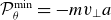
Solution without trapped electrons in the layer, demonstrating unlimited electric field growth at a finite electron temperature in the central plasma ( $T_e \approx 45$
eV,
$T_e \approx 45$
eV, $T_i \approx 8.44$
keV,
$T_i \approx 8.44$
keV, $a = 1.5$
,
$a = 1.5$
, $B_{\textrm{in}} = 0.01$
,
$B_{\textrm{in}} = 0.01$
, $\mu = 1836$
): (top) radial profiles of the electron and ion density and the electric field profile, (bottom) ion and electron azimuthal currents.
$\mu = 1836$
): (top) radial profiles of the electron and ion density and the electric field profile, (bottom) ion and electron azimuthal currents.

The numerical solution obtained in the limit of the complete absence of trapped electrons in the transition layer is shown in figure 4 ( $v_{Ti} = 0.003$
,
$v_{Ti} = 0.003$
, $\nu = v_{Ti} / v_{T_e} = 0.32$
,
$\nu = v_{Ti} / v_{T_e} = 0.32$
, $B_{\mathrm{in}} = 0.01$
,
$B_{\mathrm{in}} = 0.01$
, $a = 1.5$
). It is seen that, if the plasma is quasi-neutral at
$a = 1.5$
). It is seen that, if the plasma is quasi-neutral at $r \lt a$
, then in the transition layer, outside the region accessible to electron motion, this quasi-neutrality breaks at some radius. This leads to the electric field growth and to unlimited acceleration of ions, providing a very slow decrease in the radial profiles of their density and current. This problem was first recognised in the work of Paskievici (Reference Paskievici1962), where a similar non-physical solution was obtained for a flat transition layer. For a cylindrical plasma, a similar solution in the form of an infinitely extended charged column is realised for a stationary distribution function of the form
$r \lt a$
, then in the transition layer, outside the region accessible to electron motion, this quasi-neutrality breaks at some radius. This leads to the electric field growth and to unlimited acceleration of ions, providing a very slow decrease in the radial profiles of their density and current. This problem was first recognised in the work of Paskievici (Reference Paskievici1962), where a similar non-physical solution was obtained for a flat transition layer. For a cylindrical plasma, a similar solution in the form of an infinitely extended charged column is realised for a stationary distribution function of the form $f \propto \exp (\mathcal{E} - F(\mathcal{P}_\theta ))$
(Shustov et al. Reference Shustov, Artemyev, Vasko and Yushkov2016).
$f \propto \exp (\mathcal{E} - F(\mathcal{P}_\theta ))$
(Shustov et al. Reference Shustov, Artemyev, Vasko and Yushkov2016).
To make the solution physically meaningful, the above-mentioned works assumed the presence of a background cold plasma, the influx of electrons from which compensates the excess of the ion positive charge. A similar situation should be realised in mirror traps. The plasma in such open systems leans on the end conducting walls of the plasma receivers. If a deficit of electrons occurs on the magnetic field line running along the periphery of the plasma at the central part of the trap, the missing charge will be compensated for by electrons from the wall, which are cold in the transverse direction. Thus, in one part of the transition layer, the quasi-neutrality should be maintained by hot electrons coming from the central part of the plasma column, and in another part – by cold electrons from the wall.
5. Analysis of solutions with trapped cold electrons at different hot population temperatures
Solutions with finite electron temperature $T_e / T_i = 5.3 \times10^{-3}$
(
$T_e / T_i = 5.3 \times10^{-3}$
( $\nu = 0.32$
) (right column),
$\nu = 0.32$
) (right column), $T_e / T_i = 0.53$
(
$T_e / T_i = 0.53$
( $\nu = 0.032$
) (centre column) and
$\nu = 0.032$
) (centre column) and $T_e / T_i = 1.36$
(
$T_e / T_i = 1.36$
( $\nu = 0.02$
) (right column) in the presence of trapped cold electrons (
$\nu = 0.02$
) (right column) in the presence of trapped cold electrons ( $T_i = 8.44$
keV (
$T_i = 8.44$
keV ( $v_{Ti} = 0.003$
),
$v_{Ti} = 0.003$
), $a = 1.5$
,
$a = 1.5$
, $B_{\mathrm{in}} = 0.01$
and
$B_{\mathrm{in}} = 0.01$
and $\mu = 1836$
). Radial profiles of potentials and fields
$\mu = 1836$
). Radial profiles of potentials and fields $\varPhi$
,
$\varPhi$
, $\bar {\chi }$
,
$\bar {\chi }$
, $E_r$
and
$E_r$
and $B_z$
(upper row), of various plasma components‘ azimuthal currents (third row), their profiles of the density (second row) and pressure profiles (lower row).
$B_z$
(upper row), of various plasma components‘ azimuthal currents (third row), their profiles of the density (second row) and pressure profiles (lower row).

Now, let us consider the modification of the system of equations to be solved as follows. In those sections of the transition layer where the density of hot electrons exceeds the density of ions, the old (3.13) and (3.14) are solved. In the places where $n_i \gt n_e$
, we will add cold electrons with a density of
$n_i \gt n_e$
, we will add cold electrons with a density of $n_{ce}(r) = n_i - n_e$
to completely neutralise the space charge. Note that the excess of electron density in the initial part of the transition layer is very small, so the electric potential there can be found from the quasi-neutrality condition. In this case, the equation for the magnetic flux function should be completed with the azimuthal current created by cold electrons due to their drift in the crossed fields
$n_{ce}(r) = n_i - n_e$
to completely neutralise the space charge. Note that the excess of electron density in the initial part of the transition layer is very small, so the electric potential there can be found from the quasi-neutrality condition. In this case, the equation for the magnetic flux function should be completed with the azimuthal current created by cold electrons due to their drift in the crossed fields $J_{\varphi }^{ce} = n_{ce}E_r/B_z$
.
$J_{\varphi }^{ce} = n_{ce}E_r/B_z$
.
Solving the system of equations modified this way, we obtain the following result for the plasma density, current and pressure profiles (figure 5). Let us find out how these profiles change with the increase in electron temperature at a small bubble radius $a = 1.5$
and almost complete displacement of the magnetic field
$a = 1.5$
and almost complete displacement of the magnetic field $B_{\mathrm{in}} = 0.01$
. While the electron temperature is negligibly small compared with the ion temperature (
$B_{\mathrm{in}} = 0.01$
. While the electron temperature is negligibly small compared with the ion temperature ( $T_e \ll T_i$
,
$T_e \ll T_i$
, $\nu = v_{Ti} / v_{Te} = 0.32$
) (left column of plots in figure 5), we reproduce the same profiles that were obtained in § 2. The only difference is the appearance of an electron current, the density of which is strongly localised at the inner boundary of the transition layer and significantly exceeds the ion current density. Despite such local dominance, the total magnetic pressure jump caused by the electron current is proportional to the small electron pressure and is almost unnoticeable against the background of the field change that occurs at the ion scale due to the ion current. It is seen that this regime is still characterised by strong non-gyrotropy of the ion component, therefore due to large
$\nu = v_{Ti} / v_{Te} = 0.32$
) (left column of plots in figure 5), we reproduce the same profiles that were obtained in § 2. The only difference is the appearance of an electron current, the density of which is strongly localised at the inner boundary of the transition layer and significantly exceeds the ion current density. Despite such local dominance, the total magnetic pressure jump caused by the electron current is proportional to the small electron pressure and is almost unnoticeable against the background of the field change that occurs at the ion scale due to the ion current. It is seen that this regime is still characterised by strong non-gyrotropy of the ion component, therefore due to large $\varDelta \varPi _i$
the vacuum magnetic field pressure remains several times lower than the plasma pressure at the centre of the column, which corresponds to a very significant excess of the MagnetoHydroDynamic (MHD) limit for beta (
$\varDelta \varPi _i$
the vacuum magnetic field pressure remains several times lower than the plasma pressure at the centre of the column, which corresponds to a very significant excess of the MagnetoHydroDynamic (MHD) limit for beta ( $\beta = 2\varPi _{rr}(0) / B_v^2 \gt 1$
). If the electron temperature is increased to values comparable with ion temperature (
$\beta = 2\varPi _{rr}(0) / B_v^2 \gt 1$
). If the electron temperature is increased to values comparable with ion temperature ( $T_e \approx 0.53 T_i$
or
$T_e \approx 0.53 T_i$
or $\nu = 0.032$
in the central column of the figure 5), the two-scale structure of the transition layer becomes clearly visible. Now, the electron pressure becomes large enough, enabling the diamagnetic current at the inner boundary of the sheet to produce a noticeable jump in the magnetic field on the scale of several electron gyroradii (the width of the current sheet in the figure is shown in electron gyroradii
$\nu = 0.032$
in the central column of the figure 5), the two-scale structure of the transition layer becomes clearly visible. Now, the electron pressure becomes large enough, enabling the diamagnetic current at the inner boundary of the sheet to produce a noticeable jump in the magnetic field on the scale of several electron gyroradii (the width of the current sheet in the figure is shown in electron gyroradii $\rho _{\ast }$
and
$\rho _{\ast }$
and $\rho _v$
, calculated from the magnetic field values
$\rho _v$
, calculated from the magnetic field values $B_{\ast }$
and
$B_{\ast }$
and $B_v$
). The rest of this jump is produced by the ion current flowing through a more extended region having a width of the order of ion gyroradius. It is also seen that the non-gyrotropic addition to the ion momentum flux
$B_v$
). The rest of this jump is produced by the ion current flowing through a more extended region having a width of the order of ion gyroradius. It is also seen that the non-gyrotropic addition to the ion momentum flux $\varDelta \varPi _i$
is significantly reduced in this case. Increasing the electron temperature further (right column of images in figure 5), the jump in the magnetic field produced by electrons is increased and the role of the non-gyrotropic effect is reduced, bringing the beta of the confined plasma closer to the MHD limit
$\varDelta \varPi _i$
is significantly reduced in this case. Increasing the electron temperature further (right column of images in figure 5), the jump in the magnetic field produced by electrons is increased and the role of the non-gyrotropic effect is reduced, bringing the beta of the confined plasma closer to the MHD limit $\beta \approx 1$
. We also note that, in the limit of unimpeded inflow of cold electrons, the resulting electric field is so small that the electron drift current
$\beta \approx 1$
. We also note that, in the limit of unimpeded inflow of cold electrons, the resulting electric field is so small that the electron drift current $\boldsymbol{ E} \times \boldsymbol{B}$
is negligible compared with the diamagnetic one.
$\boldsymbol{ E} \times \boldsymbol{B}$
is negligible compared with the diamagnetic one.
6. Discussion and conclusion
In this paper, the collisionless kinetic theory of Kotelnikov (Reference Kotelnikov2020) describing the structure of the transition layer in equilibria with $\beta \sim 1$
is generalised to the case of finite electron temperature. In agreement with earlier studies that considered either a flat plasma boundary or an axially symmetric plasma without a uniform central core, obtained solutions, in the absence of trapped particles, require a violation of quasi-neutrality in the transition layer and showed an unlimited growth of the electric field with radius. Populating the transition layer with cold electrons in order to restore quasi-neutrality allows one to avoid this unphysical solution and obtain a number of conclusions that may be important for the implementation of the diamagnetic confinement regime in mirror traps.
$\beta \sim 1$
is generalised to the case of finite electron temperature. In agreement with earlier studies that considered either a flat plasma boundary or an axially symmetric plasma without a uniform central core, obtained solutions, in the absence of trapped particles, require a violation of quasi-neutrality in the transition layer and showed an unlimited growth of the electric field with radius. Populating the transition layer with cold electrons in order to restore quasi-neutrality allows one to avoid this unphysical solution and obtain a number of conclusions that may be important for the implementation of the diamagnetic confinement regime in mirror traps.
The most important effect of taking into account the electron kinetics in this problem is a decrease in the width of the transition layer, on which the rate of longitudinal particle losses depends. It turned out that, if the electron temperature in the centre of the plasma column is comparable to the ion temperature, a significant part of the total jump of the magnetic field in the transition layer occurs at its inner boundary with a width of the order of several electron gyroradii due to the diamagnetic electron current. The remaining part of the jump is produced on a scale of the order of $\rho _i$
by the diamagnetic ion current. The strong local difference between the electron and ion currents predicted by our solution can be the cause of the development of drift ion-cyclotron instabilities, which can smear the electron current sheet over a region with an ion scale. In support of the possibility of the existence of a transition layer with a sub-ion size, we can cite the PIC simulation results, obtained in a recent work (Timofeev et al. Reference Timofeev, Kurshakov and Berendeev2024). Simulations of the formation of a cylindrical equilibrium with
$\rho _i$
by the diamagnetic ion current. The strong local difference between the electron and ion currents predicted by our solution can be the cause of the development of drift ion-cyclotron instabilities, which can smear the electron current sheet over a region with an ion scale. In support of the possibility of the existence of a transition layer with a sub-ion size, we can cite the PIC simulation results, obtained in a recent work (Timofeev et al. Reference Timofeev, Kurshakov and Berendeev2024). Simulations of the formation of a cylindrical equilibrium with $\beta \sim 1$
showed that a current sheet with a size of approximately
$\beta \sim 1$
showed that a current sheet with a size of approximately $30 \rho _e$
does not change its width at half-maximum due to the development of drift instability at the ion-cyclotron frequency harmonics, and only the outer part of the transition layer, in which the ion diamagnetic current dominates, undergoes some broadening due to this effect. Thus, the obtained solutions of the collisionless kinetic equation show that the two-scale structure of the current sheet with the sub-ion size can be realised not only in equilibria of the magnetic hole type observed previously theoretically in Shustov et al. (Reference Shustov, Artemyev, Vasko and Yushkov2016), and experimentally in Li et al. (Reference Li2020), but also at the boundary of a finite-radius column with a homogeneous Maxwellian plasma, capable of completely displacing the magnetic field from itself. Taking into account the inverse dependence of the particle confinement time on the transition layer width, we can conclude that the preferable diamagnetic confinement scenarios in open traps are those in which the electron temperature is maintained at the ion temperature level.
$30 \rho _e$
does not change its width at half-maximum due to the development of drift instability at the ion-cyclotron frequency harmonics, and only the outer part of the transition layer, in which the ion diamagnetic current dominates, undergoes some broadening due to this effect. Thus, the obtained solutions of the collisionless kinetic equation show that the two-scale structure of the current sheet with the sub-ion size can be realised not only in equilibria of the magnetic hole type observed previously theoretically in Shustov et al. (Reference Shustov, Artemyev, Vasko and Yushkov2016), and experimentally in Li et al. (Reference Li2020), but also at the boundary of a finite-radius column with a homogeneous Maxwellian plasma, capable of completely displacing the magnetic field from itself. Taking into account the inverse dependence of the particle confinement time on the transition layer width, we can conclude that the preferable diamagnetic confinement scenarios in open traps are those in which the electron temperature is maintained at the ion temperature level.
If the influx of cold electrons from the walls is hampered (due to a large wall-to-mirror ratio and/or their scattering in the expander), the quasi-neutral solution with only hot electrons can be pulled much further into the transition layer. In this case, quasi-neutrality will be ensured by the appearance of a strong radial electric field, which will balance the ion pressure force and generate an electron $\boldsymbol{E}\times \boldsymbol{B}$
-drift current. It is this type of equilibrium that is realised in PIC simulations with periodic boundary conditions along the magnetic field (Park et al. Reference Park, Lapenta, Gonzalez-Herrero and Krall2019; Timofeev et al. Reference Timofeev, Kurshakov and Berendeev2024) that does not allow for the possibility of an electron influx from outside.
$\boldsymbol{E}\times \boldsymbol{B}$
-drift current. It is this type of equilibrium that is realised in PIC simulations with periodic boundary conditions along the magnetic field (Park et al. Reference Park, Lapenta, Gonzalez-Herrero and Krall2019; Timofeev et al. Reference Timofeev, Kurshakov and Berendeev2024) that does not allow for the possibility of an electron influx from outside.
Acknowledgements
The authors acknowledge useful conversations with I. Kotelnikov.
Editor Cary Forest thanks the referees for their advice in evaluating this article.
Funding
This work was supported by the Russian Science Foundation (Grant No. 24-12-00309).
Declaration of interest
The authors report no conflict of interest.


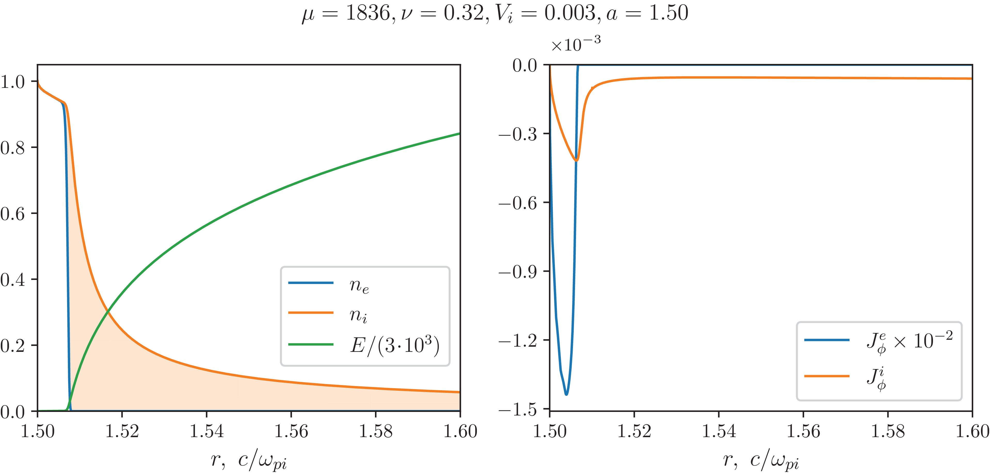


 Open access