


Introduction
The recent explosion of the number of planets detected around other stars (exoplanets, currently over 4000) by space- and ground-based missions created a great leap in the progress of the fields of exoplanetary science and astrobiology. These observations provide a boost to scientifically addressing one of the major questions of modern science ‘Are we alone in the Universe?’. Although the answer to this question is unknown, the Kepler Space Telescope's discoveries of terrestrial-type (rocky) exoplanets within circumstellar habitable zones (CHZs, the regions where standing bodies of liquid water can be present on the exoplanetary surface) around main-sequence stars have provided an important step in addressing this difficult question. An ongoing issue relates to how well the classical CHZ as calculated by Kasting et al. (Reference Kasting, Whitmire and Reynolds1993) and revisited by Kopparapu et al. (Reference Kopparapu, Ramirez, Kasting, Eymet, Robinson, Mahadevan, Terrien, Domagal-Goldman, Meadows and Deshpande2013) relates to the actual physico-chemical conditions required for the origin, development and support of life as we know it within so-called ‘Biogenic Zones’ (Airapetian et al., Reference Airapetian, Glocer, Gronoff, Hébrard and Danchi2016) or ‘Abiogenesis Zones’ (Rimmer et al., Reference Rimmer, Xu, Thompson, Gillen, Sutherland and Queloz2018).
With growing numbers of NASA (National Aeronautics and Space Administration) and ESA (European Space Agency) exoplanetary missions such as the Transiting Exoplanet Survey Satellite (TESS), the upcoming James Webb Space Telescope (JWST), Characterizing ExOPlanet Satellite (CHEOPS), the PLAnetary Transits and Oscillations of stars (PLATO), the Atmospheric Remote-sensing Infrared Exoplanet Large-Survey (ARIEL) missions, in the relatively near term we will be better equipped with high-quality observations to move from the phase of exoplanetary discovery to that of physical and chemical characterization of exoplanets suitable for life.
It is currently unknown if or when life may have begun on Earth, and possibly Mars, Venus and exoplanets, or how long those planetary bodies could remain viable for life. The principal cause of this is a lack of understanding of the detailed interaction between stars and exoplanets over geological timescales, the dynamical evolution of planetary systems and atmospheric and internal dynamics. In the last few years, there has been a growing appreciation that the atmospheric chemistry, and even retention of an atmosphere in many cases, depends critically on the high-energy radiation and particle environments around these stars (Segura et al., Reference Segura, Kasting, Meadows, Cohen, Scalo, Crisp, Butler and Tinetti2005; Domagal-Goldman et al., Reference Domagal-Goldman, Segura, Claire, Robinson and Meadows2014; Rugheimer et al., Reference Rugheimer, Kaltenegger, Segura, Linsky and Mohanty2015; Airapetian et al., Reference Airapetian, Glocer, Khazanov, Loyd, ROP, France, K, Sojka, J, Danchi, WC and Liemohn, MW2017a).
Recent studies have suggested that stellar magnetic activity and its product, astrospheric space weather (SW), the perturbations travelling from stars to planets, in the form of flares, winds, coronal mass ejections (CMEs) and energetic particles from planet hosting stars, may profoundly affect the dynamics, chemistry and exoplanetary climate (Cohen et al., Reference Cohen, Drake, Glocer, Garraffo, Poppenhaeger, Bell, Ridley and Gombosi2014; Airapetian et al., Reference Airapetian, Glocer, Gronoff, Hébrard and Danchi2016, Reference Airapetian, Jackman, Mlynczak, Danchi and Hunt2017b; Garcia-Sage et al., Reference Garcia-Sage, Glocer, Drake, Gronoff and Cohen2017; Dong et al., Reference Dong, Jin, Lingam, Airapetian, Ma and van der Holst2018).
The question of impact of stars on exoplanets is complex, and to answer it we must start with the host star itself to determine its effect on the exoplanet environment, all the way from its magnetosphere to its surface. To understand whether an exoplanet is habitable at its surface, not only do we need to understand the changes in the chemistry of its atmosphere due to the penetration of energetic particles and their interaction with constituent molecules, but also the loss of neutral and ionic species, and the addition of molecules due to outgassing from volcanic and tectonic activity. These effects will produce a net gain or loss to the surface pressure and this will affect the surface temperature, as well as a net change in molecular chemistry. Therefore, due to the complexity of the problem, we should work with a set of interlinked research questions, all of which contribute pieces to the answer, with contributions from various disciplines involved in each topic.
To quantify the effects of stellar ionizing radiation including soft X-ray and extreme ultraviolet, EUV (100–920 Å), later referred to as XUV fluxes from superflares detected by the Kepler mission on exoplanetary systems, specifically, on close-in exoplanets around low luminosity M dwarf stars, we need to examine what do we know about the impact of SW from our own star on Venus, Mars and Earth, the only inhabited planet known to us. How can we apply lessons learned from the extreme SW events to understand how exoplanets are affected by their host stars? Can heliophysics science with its methodologies and models developed to describe the effects of solar flares, CMEs as the factors of SW, on Venus, Earth and Mars be expanded to address the extreme conditions on exoplanets around young solar-like stars and close-in exoplanets around active F, G, K and M dwarfs? These questions are of critical importance as the major factors of habitability of exoplanets.
In this paper, we present the roadmap to study various aspects of star–planet interactions in a global exoplanetary system environment with a systematic, integrated approach using theoretical, observational and laboratory methods combining tools and methodologies of four science disciplines: astrophysics, heliophysics, planetary and Earth science as presented in Fig. 1. The components of the presented roadmap had been discussed during the NASA Nexus for Exoplanetary System Science (NExSS) sponsored Workshop Without Wall ‘Impact of Exoplanetary Space Weather on Climate and Habitability’ and recent white papers submitted to the US National Academy of Sciences for Exoplanet Science Strategy, Astrobiology Science Strategy and Astronomy and Astrophysics (Astro2020) calls (see Airapetian et al., Reference Airapetian, Danchi, Dong, Rugheimer, Mlynczak, Stevenson, Henning, Grenfell, Jin, Glocer, Gronoff, Lynch, Johnstone, Lueftinger, Guedel, Kobayashi, Fahrenbach, Hallinan, Stamenkovic, Cohen, Kuang, van der Holst, Manchester, Zank, Verkhoglyadova, Sojka, Maehara, Notsu, Yamashiki, France, Lopez Puertas, Funke, Jackman, Kay, Leisawitz and Alexander2018a, Reference Airapetian, Adibekyan, Ansdell, Cohen, Cuntz, Danchi, Dong, Drake, Fahrenbach, France, Garcia-Sage, Glocer, Grenfell, Gronoff, Hartnett, Henning, Hinkel, Jensen, Jin, Kalas, Kane, Kobayashi, Kopparapu, Leake, López-Puertas, Lueftinger, Lynch, Lyra, Mandell, Mandt, Moore, Nna-Mvondo, Notsu, Maehara, Yamashiki, Shibata, Oman, Osten, Pavlov, Ramirez, Rugheimer, Schlieder, Schnittman, Shock, Sousa-Silva, Way, Yang, Young and Zank2018b, Reference Airapetian, Adibekyan, Ansdell, Alexander, Barklay, Bastian, Boro Saikia, Cohen, Cuntz, Danchi, Davenport, DeNolfo, DeVore, Dong, Drake, France, Fraschetti, Herbst, Garcia-Sage, Gillon, Glocer, Grenfell, Gronoff, Gopalswamy, Guedel, Hartnett, Harutyunyan, Hinkel, Jensen, Jin, Johnstone, Kahler, Kalas, Kane, Kay, Kitiashvili, Kochukhov, Kondrashov, Lazio, Leake, Li, Linsky, Lueftinger, Lynch, Lyra, Mandell, Mandt, Maehara, Miesch, Mickaelian, Mouschou, Notsu, Ofman, Oman, Osten, Oran, Petre, Ramirez, Rau, Redfield, Réville, Rugheimer, Scheucher, Schlieder, Shibata, Schnittman, Soderblom, Strugarek, Turner, Usmanov, Van Der Holst, Vidotto, Vourlidas, Way, Wolk, Zank, Zarka, Kopparapu, Babakhanova, Pevtsov, Lee, Henning, Colón and Wolf2019a and the link at https://nexss.info/community/woskshops/workshop-without-walls-exoplanetary-scape-weather-climate-and-habitability).
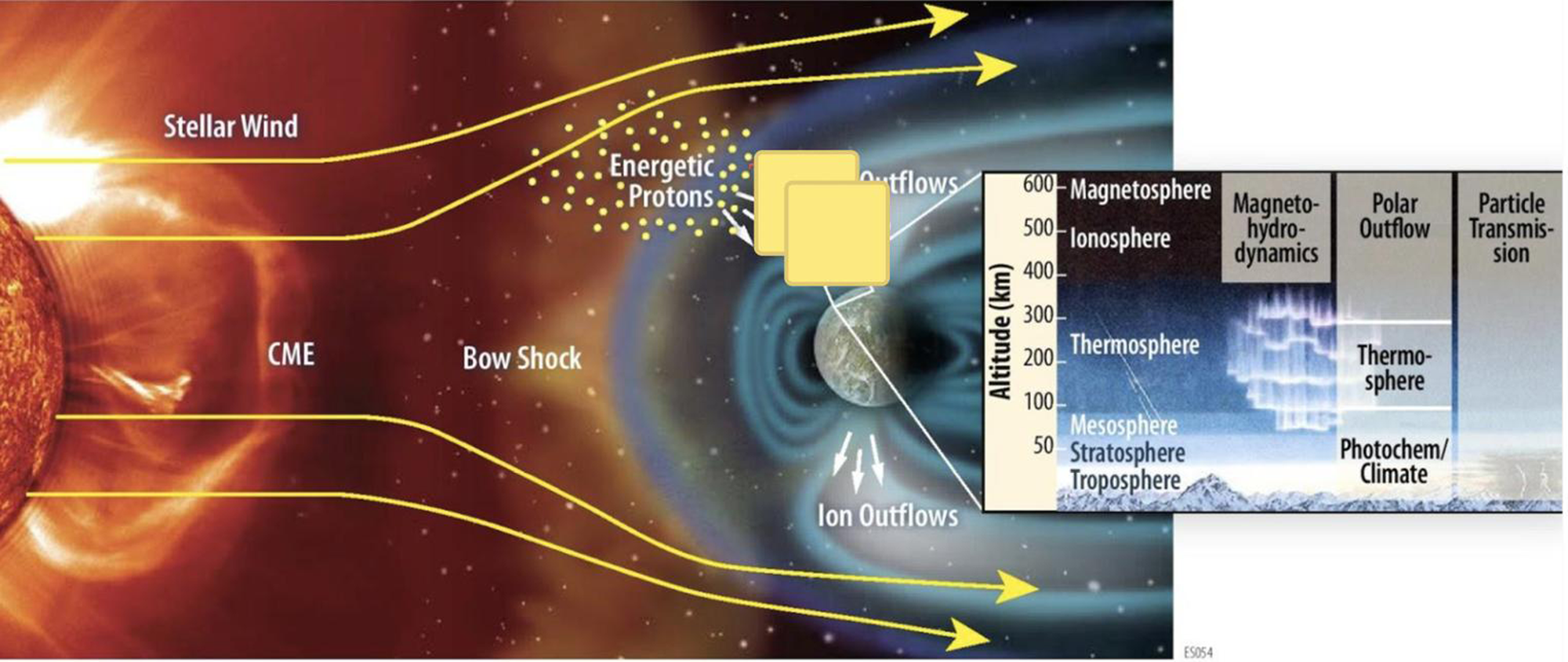
Fig. 1. Schematic view of the complex exoplanetary SW system that incorporates the physical processes driving stellar activity and associated SW including stellar flares, CMEs and their interactions with an exoplanetary atmosphere driven by its internal dynamics. While stellar winds and CMEs affect the shape of an exoplanetary magnetosphere, XUV and energetic particles accelerated on CME-driven shocks enter the atmosphere. The combined effects of XUV, stellar winds and CMEs drive outflows from the exoplanetary atmosphere. These processes are controlling factors of exoplanetary climate and habitability.
We describe recent progress and challenges in understanding the nature of solar and stellar magnetic activity and associated SW processes from the modern Sun, the young Sun (at the time when life started on Earth) and from other cool (K through M spectral type) stars. We discuss the physical processes that drive the interaction of SW with the Earth, Mars and Venus and the implications for exoplanets around active stars including internal dynamics that drive outgassing. This review paper consists of Introduction and nine sections.
Section ‘Drivers and signatures of space weather from the Sun’ discusses the structures of global solar corona and the solar wind, properties of solar flares, CMEs and solar-energetic particle (SEPs) and their observational signatures.
In section ‘Space Weather from active stars’, we review recent observations and modelling efforts of coronae, winds and superflares from young solar-type planet hosting stars.
In section ‘Impact of space weather effects on modern Earth, Venus and Mars’, we present a review of current observations and theoretical models of atmospheric erosion and chemical changes in the atmospheres of modern Earth, Mars and Venus caused by XUV emission from solar flares, CMEs and SEP events.
Section ‘Space weather impact on (exo)planetary systems: atmospheric loss’ highlights the current understanding of the effects of solar and stellar XUV-driven emission and the dynamic pressure exerted by solar and stellar winds, CMEs on atmospheric escape processes from early Earth, Mars, Venus and terrestrial-type exoplanets including exoplanets around Proxima Centauri and TRAPPIST 1.
Section ‘Impact of space weather on (exo)planetary atmospheric chemistry’ discusses the impact of SEP events on atmospheric chemistry of early Earth- and SEP-driven surface dosages of ionizing radiation of terrestrial-type exoplanets.
Section ‘Space weather, habitability and biosignatures’ reviews the impact of SW in the form of XUV fluxes and SEP events on climate-related processes, exoplanetary habitability and the properties of atmospheric biosignatures from terrestrial-type exoplanets orbiting K-G-M stars.
Section ‘Internal dynamics of rocky exoplanets and the influence on habitability’ discusses interior dynamics of terrestrial-type planets as a function of their chemical composition, mass, size and explores the potential of volcanic and tectonic activity which plays a key role for atmospheric evolution. It also discusses current efforts in magnetohydrodynamic (MHD) modelling of exoplanetary dynamos and their effects on habitability.
In section ‘Observational methods and strategies for the detection of habitable planets’, we present observational strategies for detection of habitable environments on terrestrial-type exoplanets around different main-sequence stars and review progress in recent observations of exoplanets by the Kepler Space Telescope, HST and ground-based telescopes which employ transit spectroscopy, direct imaging, radial velocity and gravitational lensing. We also discuss a roadmap to detect biosignatures using stellar interferometers and the next generation ground based and space telescopes: TESS, CHEOPS, JWST, PLATO 2.0, ARIEL, the E-ELT, LUVOIR, ORIGINS, LYNX and HabEx.
Section ‘Conclusions: future prospects and recommendations’ discusses future prospects and provides recommendations for the next steps in understanding of various aspects of star–planet interactions, the ways they affect planetary habitability and observational strategies to detect habitable worlds in the coming decade.
Drivers and signatures of space weather from the Sun
Our Sun is a major source of energy for much of life on Earth. Our central star was formed from a collapsing protostellar cloud 4.65 billion years ago. The Solar system formed from the protoplanetary disc left after the Sun's birth was bombarded by a vast amount of energy in the form of electromagnetic radiation, solar wind, magnetic clouds (MC), shock waves and energetic electrons and protons. Recent heliospheric missions including the Solar and Heliospheric Observatory (SOHO), the Solar Dynamic Observatory (SDO) and the Solar Terrestrial Relations Observatory (STEREO) have provided a wealth of information about our magnetic star. This has helped to recover statistical information about the spatial and temporal relationship between eruptive events occurring in the solar corona and provided clues to the physical mechanisms driving their underlying processes.
The primary output from the Sun is in the energy flux in the form of electromagnetic and mass emissions, ultimately powered by the thermonuclear reactions in the solar interior that convert hydrogen to helium and amplified by the magnetic dynamo that generates and transports magnetic fields to surface and the atmosphere. The steady or quiescent electromagnetic emission in the visible and infrared bands supports life on Earth, while solar XUV flux creates the ionosphere around Earth and affects its upper atmospheric chemistry.
Electromagnetic emission can also be transient, in the form of solar flares at almost all wavelengths. Solar flares cause transient disturbances in Earth's ionosphere. The mass emission occurs in the form of steady two-component solar wind with speeds in the range of 300–900 km s−1 and as CMEs that have speeds ranging from <100 to >3000 km s−1 (e.g. Gopalswamy, Reference Gopalswamy2016). Fast CMEs (faster than the magnetosonic speed in the corona and interplanetary (IP) medium) drive MHD shocks that are responsible for the copious acceleration of electrons, protons and heavy ions commonly referred to as SEPs. Energetic protons are known to significantly impact Earth's atmosphere. CMEs are magnetized plasmas with a flux rope structure, which when impacting a magnetized plasma can lead to geomagnetic storms (GM) that have serious consequences in the planetary magnetosphere/ionosphere/atmosphere. Solar wind magnetic structures can also result in moderate magnetic storms. Thus, SEPs and magnetic storms associated with CMEs are considered to be severe SW consequences of solar eruptions on the technological infrastructure of the modern world (Schrijver et al., Reference Schrijver, Kauristie, Aylward, Denardini, Gibson, Glover, Gopalswamy, Grande, Hapgood, Heynderickx, Jakowski, Kalegaev, Lapenta, Linker, Liu, Mandrini, Mann, Nagatsuma, Nandy, Obara, Paul O'Brien, Onsager, Opgenoorth, Terkildsen, Valladares and Vilmer2015). Flares and CMEs are formed within closed solar-magnetic regions (active regions), while the solar wind originates from open field regions. Magnetic regions on the Sun also modulate the amount of visible radiation emitted by the solar plasma, because of a combination of sunspots and the surrounding plages (e.g. Solanki et al., Reference Solanki, Krivova and Haigh2013).
Origin and patterns of solar-magnetic activity: global solar corona
The outermost layer of the Sun, the solar corona, is the hottest atmospheric region of the Sun heated to ~1–2 MK, which is by a factor of 200 hotter than the solar photosphere. This suggests that the solar corona is heated from the lower atmosphere of the Sun driven by the surface (photospheric) magnetic-field supplying and dissipating its energy in the upper atmospheric heating. Two possible mechanisms of heating include upward propagating magnetic waves (in the form of Alfvén waves) generated by photospheric convection and nanoflares, magnetic reconnection driven explosions releasing energy of ~1020 erg (De Pontieu et al., Reference De Pontieu, Rouppe van der Voort, McIntosh, Pereira, Carlsson, Hansteen, Skogsrud, Lemen, Title, Boerner, Hurlburt, Tarbell, Wuelser, De Luca, Golub, McKillop, Reeves, Saar, Testa, Tian, Kankelborg, Jaeggli, Kleint and Martinez-Sykora2014). The coronal heating varies across the solar surface forming a diffuse corona (see left panel of Fig. 2) and active regions (white concentrated regions above sunspots).

Fig. 2. Left panel: NASA/SDO image of the magnetic Sun in the 211 Å band with superimposed magnetic-field lines interconnecting active regions (NASA/SDO). Right panel: Global solar corona highlighted during ‘Great American’ solar eclipse of 17 August 2017 (Copyright: Nicolas Lafaudeux (https://apod.nasa.gov/apod/ap180430.html)).
The left panel of Fig. 2 shows the SDO image in the 211 Å band (representative T ~ 2.5 MK) (https://sdo.gsfc.nasa.gov/gallery/main/item/37). The superimposed coronal magnetic-field lines show that the magnetic field in the solar corona is organized into small (up to a few tens of kilometres as resolved by ground-based solar telescopes) and large scale (comparable to the solar radius) structures connecting active regions, with their complexity varying with the solar cycle. The solar corona represents a magnetically controlled environment, and thus plasma structures observed on the solar active regions trace magnetic-field lines (bright regions on the left panel of Fig. 2). The right panel of Fig. 2 shows the solar corona during the solar eclipse of 17 August 2017. Its polar regions show open rays that are solar coronal holes, the regions of the open magnetic flux with lower density and temperature plasma that appear as dark regions in X-ray and EUV images (see the lower hole in the left panel of Fig. 2). The open magnetic flux and coronal structures evolve with the phase of the solar cycle (from solar minimum of magnetic activity to solar maximum) running through the polarity flip every 11 years. While global magnetic field during minimum of activity can be relatively well represented by dipole field (close to the global field represented in the left panel of Fig. 2), it becomes less organized with the presence of quadrupole and other multipole components (Kramar et al., Reference Kramar, Airapetian and Lin2016).
During solar maximum coronal holes migrate from low latitudes towards the equator with the progression of the solar cycle, while during solar minimum they can be mostly found in the polar regions (McIntosh et al., Reference McIntosh, Wang, Leamon, Davey, Howe, Krista, Malanushenko, Markel, Cirtain, Gurman, Pesnell and Thompson2014). Solar coronal streamers near solar maximum are mostly located near the polar regions (see the right panel of Fig. 2) of the Sun and can be described with higher magnetic multipole moments associated with coronal active regions in addition to the dipole component of the global magnetic field. During solar minimum, solar streamers are formed near the equator and are not associated with coronal active regions. They can be described by mostly dipolar field component inclined 10° to the solar rotation axis with the heliospheric current concentrated in the heliospheric current sheet above the dipolar magnetic field at ~2.5 R⊙ (Zhao and Hoeksema, Reference Zhao and Hoeksema1996).
Static solar corona extends into IP space as the supersonic outflow known as the solar wind first predicted by Parker (Reference Parker1958). The solar wind forms a background for propagation of coronal disturbances including CMEs and associated SEP events, and thus constitutes the major component of SW. Remote sensing and in-situ measurements demonstrate that near solar minimum the solar wind has a bi-modal structure. The fast wind represents a high-speed (up to 800 km s−1 at 1 AU) low density (1–5 cm−3) outflow emanating from the lower solar corona around polar regions and is associated with unipolar coronal holes. The slow wind (~350–400 km s−1) is a factor of 3–10 denser and forms above the low latitude regions associated with large-scale equatorial structures known as coronal streamer belt with the mass loss rate of 2 × 10⁻¹⁴ M⊙ per year (McComas et al., Reference McComas, Velli, Lewis, Acton, Balat-Pichelin, Bothmer, Dirling, Feldman, Gloeckler, Habbal, Hassler, Mann, Matthaeus, McNutt, Mewaldt, Murphy, Ofman, Sittler, Smith and Zurbuchen2007). Driven by the solar rotation, the high- and low-wind components form alternating streams moving outwards into IP space in an Archimedean spiral. At distance around 1 AU or farther away from the Sun, the high-speed streams eventually overtake the slow-speed flows and form regions of enhanced density and magnetic field known as co-rotating interaction regions (CIRs). These compressed interstream regions play an important role in SW as a trigger of GM.
Thus, it is important to understand the physics of the dynamic solar wind as a major factor of the impact of the associated variable SW on the Earth's magnetosphere. Historically, the first thermally driven coronal solar-wind model was developed by Parker (Reference Parker1958). It could satisfactory describe the slow solar-wind component but failed to explain the fast wind component. In order to explain the fast wind component, an additional momentum term is required (Usmanov et al., Reference Usmanov, Goldstein, Besser and Fritzer2000; Airapetian et al., Reference Airapetian, Carpenter and Ofman2010; Ofman, Reference Ofman2010; Airapetian and Cuntz, Reference Airapetian, Cuntz, Ake and Griffin2015). Recently developed data-driven global MHD models can successfully reproduce the overall global structure of the solar corona, the solar wind and incorporate the physical processes of heating and acceleration of the solar wind with the initial state and boundary conditions directly derived from observations (van der Holst et al., Reference van der Holst, Sokolov, Meng, Jin, Manchester, Tóth and Gombosi2014; Oran et al., Reference Oran, Landi, van der Holst, Sokolov and Gombosi2017; Reiss et al., Reference Reiss, MacNeice, Mays, Arge, Möstl, Nikolic and Amerstorfer2019).
Origin and patterns of solar-magnetic activity: transient events
Observations and characterization of solar activity in the form of varying numbers of sunspots on its disc have been performed since 1600s. Herschel (Reference Herschel1801) recognized periods of low and high sunspot activity and correlated the low sunspot activity with high wheat prices in England. Decades later, Schwabe (1843) in his pursuit of a hypothetical planet closer to the Sun than Mercury, discovered a 10-year periodicity in the sunspot number; in 1850, the periodicity was confirmed by Rudolf Wolf and refined to be about 11 years. This discovery has long-lasting implications because the impact on planets accordingly waxes and wanes. The discovery of magnetic fields in sunspots by Hale (Reference Hale1908) led to the identification of 22-year magnetic cycle of the Sun (Hale cycle). Sunspots typically appear in pairs with leading and following spots having opposite magnetic polarity in a given hemisphere; the polarity is switched in the other hemisphere. This pattern is maintained over the 11-year sunspot cycle (also known as the Schwabe cycle). In the new cycle, the polarities of the leading and following polarities are switched in both hemispheres. The polarity switching is referred to as the Hale–Nicholson law. Other periodicities are also known, especially the Gleissberg cycle with a periodicity in the range of 80–100 years (see e.g. Pertrovay, Reference Pertrovay2010). Finally, solar activity has grand minima and maxima over millennial timescales that do not seem to be periodic. The well-known example is the Maunder Minimum discovered by Eddy (Reference Eddy1976), when the sunspot activity almost vanished during 1640–1715 AD. Sunspots were observed for only about 2% of the days in this interval. Estimates show that the Sun has spent <20% of the time in grand minima and <15% of the time in grand maxima in the Holocene (see Usoskin, Reference Usoskin2017 for a review).
The magnetic field associated with sunspots is known as the toroidal component of the solar-magnetic field. The other component is the poloidal magnetic field, which peaks during the minimum phase of a solar cycle. The polarity of the poloidal field reverses during the maximum phase of the solar cycle (Babcock and Babcock, Reference Babcock and Babcock1955; Babcock, Reference Babcock1959). Figure 3 shows the toroidal (low latitude) and poloidal (high latitude) components using longitudinally averaged photospheric magnetic field and the microwave brightness temperature, which is a proxy to the magnetic-field strength. The data correspond to part of solar cycle 22 (before the year 1996), whole of cycle 23 (1996–2008) and most of cycle 24 (after the year 2008). Note that the toroidal field starts building up when the poloidal field starts declining and vice versa. The poloidal field development is clearly connected to the evolution of the sunspot fields (local peaks at low latitudes) via plumes, which consist of the eastern parts of sunspot regions moving towards the poles as a consequence of the Joy's law.
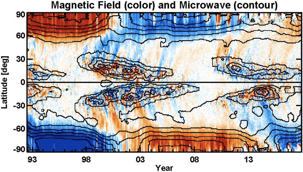
Fig. 3. The toroidal and poloidal components of the solar-magnetic field (blue – negative; red – positive). The contours represent microwave brightness temperature at 17 GHz obtained from the Nobeyama Radioheliograph (contour levels: 9400, 9700, 10 000, 10 300, 10 600, 10 900, 11 200, 11 500, 11 800, 12 100 K). The field distribution between ±30° latitude represents the toroidal field, while that poleward of ~60° latitudes represents the poloidal field. Data updated from Gopalswamy et al. (Reference Gopalswamy, Yashiro and Akiyama2016).
The sunspot cycle can thus be explained by a magnetic dynamo model in which the poloidal and toroidal fields mutually generate each other (see e.g. Charbonneau, Reference Charbonneau2010, for a review) in the presence of differential rotation, convective motion beneath the surface and meridional circulation. Filaments (also known as prominences when appearing at the solar limb) are another important phenomena occurring generally in the mid-latitudes but move towards the poles during the maximum phase. Filaments usually mark the polarity inversion lines in magnetic regions either in sunspot regions or in bipolar magnetic regions without sunspots. The disappearance of the polar crown filaments roughly marks the time of polarity reversal at the poles.
The extension of sunspot regions into the outermost region of the Sun, solar corona is known as an active region. Some active regions can be without sunspots (the quiescent filament regions). In X-rays and EUV, active regions appear as a collection of loops, which are thought to be magnetic in nature. Solar eruptions, a collective term representing energy release in the form of flares and CMEs, occur in active regions. The energy release happens in the form of heating, particle acceleration and mass motion. Accelerated particles from the corona travel along magnetic-field line towards the Sun produce various signatures of flares from radio to gamma-ray wavelengths. Non-thermal particles precipitating into the photosphere cause enhanced optical emission, which was originally recognized as solar flares by Carrington (Reference Carrington1859) and Hodgson (Reference Hodgson1859). Chromospheric signatures of solar flares are readily observed in H-α in the form of flare ribbons and post-eruption arcades. Soft X-rays are sensitive indicators of flare heating and the intensity of flare X-rays can vary over six orders of magnitude. Non-thermal electrons propagating away from the Sun produce various types of radio bursts from decimetric to kilometric wavelengths. Type-III bursts generally indicate electrons propagating from the flare site into open magnetic-field lines. Another source of particle acceleration is the shocks formed ahead of CMEs that can form very close to the Sun (0.2 Rs above the solar surface (Gopalswamy et al., Reference Gopalswamy, Xie, Mäkelä, Yashiro, Akiyama, Uddin, Srivastava, Joshi, Chandra, Manoharan, Mahalakshmi, Dwivedi, Jain, Awasthi, Nitta, Aschwanden and Choudhary2013)) and survive to 1 AU and beyond. Electrons accelerated at the shock front produce type-II radio bursts (Gopalswamy, Reference Gopalswamy, Rucker, Kurth, Louarn and Fischer2010). Type-II radio bursts are the second most intense class in the 30 MHz to 30 m kHz band (metric band). Their frequency varies in time with the frequency drift from 200 MHz to 30 MHz in about 5 min in the solar corona, and in IP space from 30 MHz to 30 kHz in 1–3 days. There is strong evidence that such emission during type-II events is generated near the first and second harmonics of the local plasma frequency upstream of the shock via the plasma mechanism: non-thermal electrons accelerated at the shock generate Langmuir waves at the local plasma frequency that get converted into electromagnetic radiation at the fundamental and second harmonic of the local plasma frequency (Cairns, Reference Cairns2011). The same shock accelerates protons to very high energies and hence is thought to be the primary source of SEP events observed in the IP space.
CMEs and flares can be ultimately traced to magnetic regions on the Sun. The CME kinetic energy is typically the largest among various components of the energy release (e.g. Emslie et al., Reference Emslie, Dennis, Shih, Chamberlin, Mewaldt, Moore, Share, Vourlidas and Welsch2012). CME kinetic energies have been observed to have values exceeding ~1033 erg. The only plausible source of energy for eruption is likely to be magnetic in nature (e.g. Forbes, Reference Forbes2000). It is thought that the closed magnetic-field lines in the active region store free energy when stressed by photospheric motions and the energy can be released by a trigger mechanism involving magnetic reconnection.
Flares and CMEs generally are closely related: flares represent plasma heating while CMEs represent mass motion resulting from a common energy release. This is especially true for large flares and energetic CMEs. Small flares may not be associated with CMEs and occasionally large CMEs can occur with extremely weak flares, especially when eruptions occur outside sunspot regions (Gopalswamy et al., Reference Gopalswamy, Akiyama, Mäkelä, Yashiro, Xie, Thakur and Kahler2015). Even X-class flares can occur without CMEs, but in these cases, no metric radio bursts or non-thermal particles observed in the IP medium, suggesting that the only thing that escapes is the electromagnetic radiation (Gopalswamy et al., Reference Gopalswamy, Akiyama and Yashiro2009). Flares without CMEs are known as confined flares as opposed to eruptive flares that involve mass motion.
Space weather: solar flares, CMEs and SEPs
Solar eruptions are one of the major sources of SW at Earth and other planets. Solar flares suddenly increase the X-ray and EUV input to the planetary atmosphere by many orders of magnitude. They are also sources of energetic electrons and protons accelerated at the flare reconnection sites in the solar corona forming short-lived SEP events known as impulsive events with maximum particle energy of ~10 MeV (Kallenrode, Reference Kallenrode2003). Another type of energetic particle observed in IP space, gradual SEP events, last over 1 day, which are accelerated to energies over a few GeV per nucleon. These events are associated with CME-driven shocks forming in the outer corona at ≥2R Sun. Particles are accelerated via diffusive shock acceleration mechanism based on Fermi I acceleration via multiple scattering of particles on plasma turbulent homogeneities as they cross the shock front (Zank et al., Reference Zank, Rice and Wu2000; Li et al., Reference Li, Shalchi, Ao, Zank and Verkhoglyadova2012).
On the other hand, CME and associated SEP events have a much longer-term impact from the time the shock forms near the Sun to times well beyond shock arrival at the planet. In the case of Earth this duration can be several days. SEPs precipitate in the polar region and participate in atmospheric chemical processes. When the shock arrives at Earth, a population of locally accelerated energetic particles known as energetic storm particles is encountered. If a GM ensues after the shock (due to sheath and/or CME) then additional particles are accelerated within the magnetosphere. Thus, the ability of a CME to accelerate SEPs and to cause magnetic storms are the most important consequences of SW. Fast CME-driven IP shocks are associated with narrow band metric radio burst emissions (1–14 MHz) and broad band radio emissions (<4 MHz) called IP type-II events.
The continuous CME observations over the past two decades with the simultaneous availability of SEP observations, IP shock observations and IP type-II event data over the past two decades have helped us characterize CMEs that cause SEP events and GM. Figure 4 shows a cumulative distribution of CME speeds observed by SOHO coronagraphs. The average speed of all CMEs is ~400 km s−1. All populations of CMEs marked on the plot are fast events (over 600 km s−1): metric type-II radio bursts (m2) due to CME-driven shocks in the corona at heliocentric distances <2.5 R⊙; MC that are IP CMEs with a flux rope structure; IP CMEs lacking flux rope structure (ejecta, EJ); shocks (S) ahead of IP CMEs detected in the solar wind; GM caused by CME magnetic field or shock sheath; halo CMEs (Halo) that appear to surround the occulting disc of the coronagraph and propagating Earthward or anti-Earthward; decametre-hectometric (DH) type-II radio bursts indicating electron acceleration by CME-driven shocks in the IP medium; SEP events caused by CME-driven shocks; ground-level enhancement (GLE) in SEP events indicating the presence of GeV particles. It must be noted that MC, EJ, GM and Halo are related to the internal structure of CMEs in the solar wind, while the remaining are all related to the shock-driving capability of CMEs and hence particle acceleration. Note that SEP-causing CMEs have an average speed that is four times larger than the average speed of all CMEs. CMEs causing magnetic storms have an average speed of ~1000 km s−1, which is more than two times the average speed of all CMEs. It must be noted that these CMEs originate close to the disc centre of the Sun and hence are subject to severe projection effects. The projected speeds are likely to be similar to those of SEP-causing CMEs. SEP-causing CMEs form a subset of CMEs that produce DH type-II bursts because the same shock accelerates electrons (for type-II bursts) and SEPs. SEPs in the energy range 10–100 MeV interact with various layers of Earth's atmosphere, while the GeV particles reach the ground. Note that only about 3000 CMEs belong to the energetic populations ranging from metric type-II bursts to GLE events, suggesting that only ~15% of CMEs are very important for adverse SW, while the remaining 85% form significant inhomogeneities in the background solar wind.
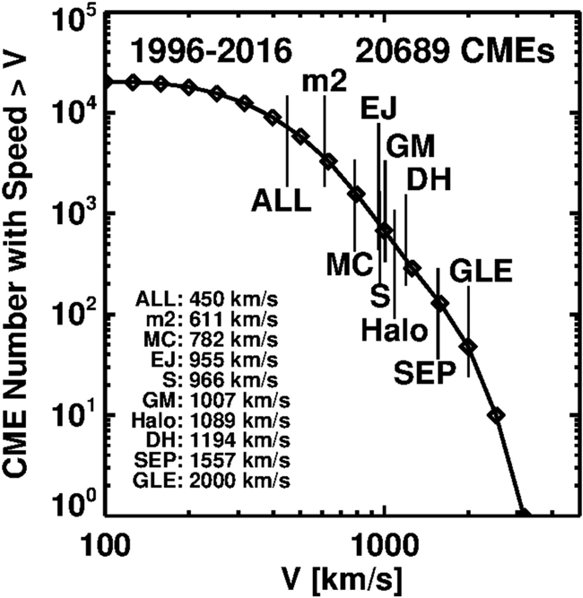
Fig. 4. Cumulative distribution of CME sky-plane speeds (V) from the SOHO coronagraphs during 1996–2016. More than 20 000 CMEs catalogued at the CDAW Data Center (https://cdaw.gsfc.nasa.gov) have been used to make this plot. The average speeds of CME populations associated with various coronal and IP phenomena are marked on the plot. Updated from Gopalswamy (Reference Gopalswamy and Buzulukova2017).
Another point to be noted is that CMEs from the Sun do not have speeds exceeding ~4000 km s−1. This limitation is most likely imposed by the size of solar active regions, their magnetic content, and the efficiency with which the free energy can be converted into CME kinetic energy. Gopalswamy (Reference Gopalswamy and Buzulukova2017) estimated magnetic energy up to ~1036 erg can be stored in solar active regions and a resulting CME can have a kinetic energy of up to 1035 erg. Such events may occur once in several thousand years. Note that the highest kinetic energy observed over the past two decades is ~4 × 1033 erg.
Figure 5(a) shows the relation between sunspot number, numbers of large SEP events, major GM, major X-ray flares and fast CMEs. There is a general pattern in which fast CMEs and major flares occur more frequently during the maximum phase of solar activity. Accordingly, the SW events also occur in correlation with the sunspot number. There are clearly periods when there is discordant behaviour between CMEs and flares, but there is generally a better correlation between CMEs, SEPs and magnetic storms.
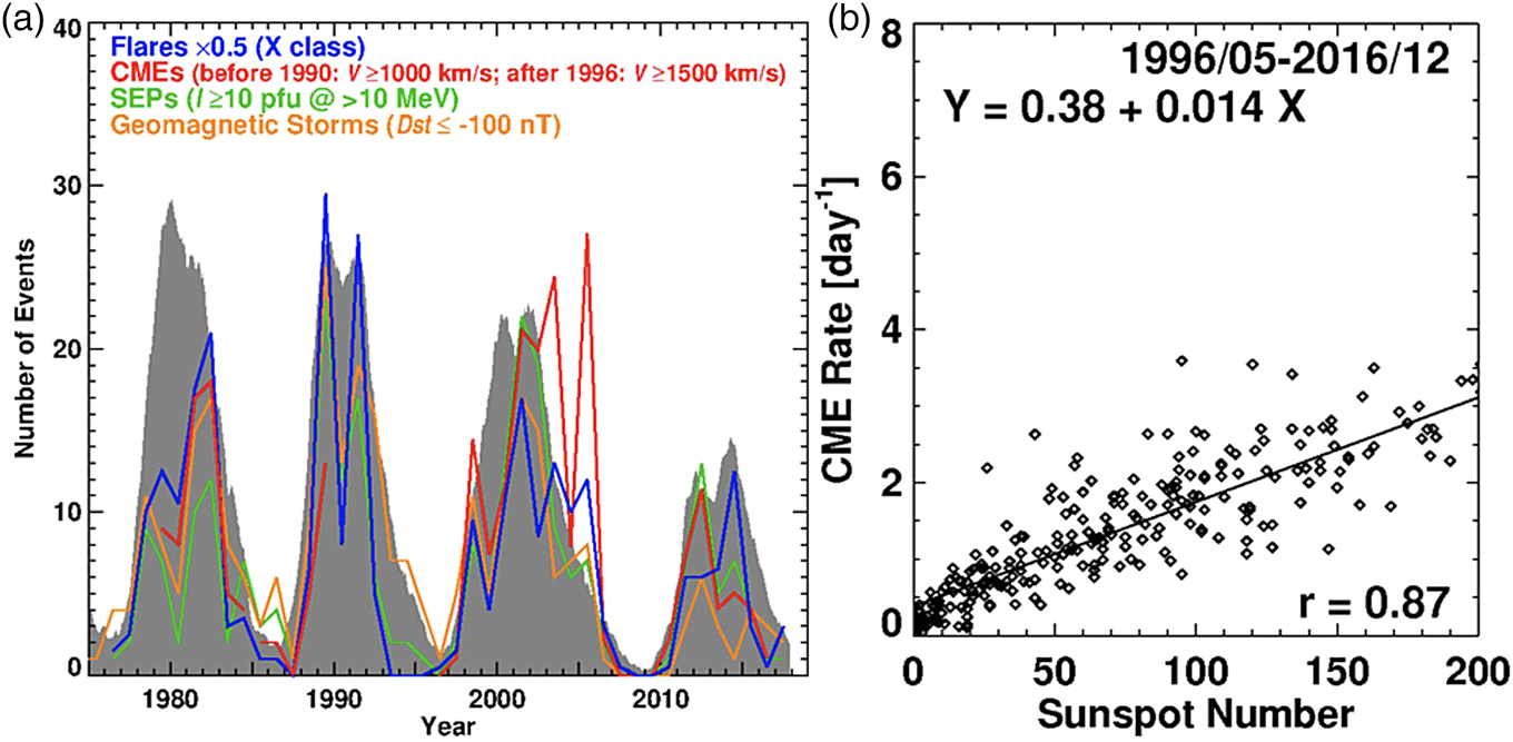
Fig. 5. (a) Solar-cycle variation of X-class soft X-ray flares, fast CMEs, large SEP events and major GM. All the vent types generally follow the solar cycle represented by the sunspot number (grey). (b) Scatter plot between the daily CME rate and sunspot number during 1996–2016.
The close connection between sunspot number and SW events can be understood from the fact that large magnetic energy required to power the CMEs can be stored only in sunspot regions. Figure 5(b) shows that the CME rate is higher during high sunspot number, with a correlation coefficient of 0.87. The correlation is high, but not perfect. In fact, Gopalswamy et al. (Reference Gopalswamy, Akiyama, Yashiro, Mäkelä, Hasan and Rutten2010) showed that during the rising and declining phases of the solar cycle, the CME rate – sunspot number correlations are very high (r ~ 0.90), but it is slightly lower (~0.70) during the maximum phase. This is because CMEs also originate from non-spot magnetic regions (quiescent filament regions), which are very frequent in the maximum phase.
Space weather from active stars
Recent X-ray and UV missions including CHANDRA, XMM-NEWTON, the Hubble Space Telescope and the Kepler Space Telescope have opened new windows onto the lives of stars resembling our Sun at various phases of evolution. This has provided a unique opportunity to infer the magnetic properties of planet hosting stars.
The evolutionary history of the Sun and active stars can be reconstructed by studying atmospheric signatures of solar-like stars at various phases of evolution. Physical properties such as rotation velocity and magnetic activity of young solar-like stars strongly depend on age (see, e.g. Shaviv, Reference Shaviv2003; Cohen et al., Reference Cohen, Drake and Kóta2012; Wood et al., Reference Wood, Muller, Redfield and Edelman2014; Johnstone et al., Reference Johnstone, Güdel, Stökl, Lammer, Tu, Kislyakova, Lüftinger, Odert, Erkaev and Dorfi2015a, Reference Johnstone, Güdel, Brott and Lüftinger2015b, Reference Johnstone, Güdel, Lüftinger, Toth and Brott2015c; Airapetian and Usmanov, Reference Airapetian and Usmanov2016). This section describes recent observational and modelling efforts in reconstructing XUV emission and stellar wind properties of active planet hosting stars as their output plays a crucial role in dynamics of exoplanetary atmospheres.
Coronal properties of active stars
In general, young Sun-like stars have higher rotation velocities, a higher magnetic activity as well as significantly higher mass loss rates (see, e.g. Güdel et al., Reference Güdel, Guinan and Skinner1997; Wood et al., Reference Wood, Müller, Zank and Linsky2002; Güdel and Nazé, Reference Güdel and Nazé2009; Cleeves et al., Reference Cleeves, Adams and Bergin2013). Furthermore, observations of young Sun-like stars have shown the signatures of large magnetic spots that are concentrated at higher latitudes (Strassmeier, Reference Strassmeier2001) than the sunspots observed on the current Sun. It is also known that the rotation velocity of a star is correlated with its magnetic activity specified by X-ray flux (Güdel, Reference Güdel2007). Rapidly rotating young solar-type stars show stronger surface magnetic field (a few hundreds of G) and two-to-three orders of magnitude greater XUV flux than the modern Sun according to solar analogue data (Ribas et al., Reference Ribas, Guinan, Gudel and Audard2005).
While the long-term evolution of the Sun's bolometric radiation is quite well understood from calculations of the Sun's internal structure and nuclear reactions (e.g. Sackmann and Boothroyd, Reference Sackmann and Boothroyd2003), the evolution of the high-energy radiation is less clear. This emission short-ward of approximately 150–200 nm originates in magnetically active regions at the stellar chromospheric, transition region and corona (in the order of increasing height and temperature). The heating of the plasma in these regions may be caused by the dissipation of magnetic energy as it is observed on the Sun (see section ‘Origin and patterns of solar-magnetic activity: global solar corona’).
The long-term evolution of the magnetically induced high-energy radiation is related to solar/stellar rotation rate with chromospheric emission also increasing with the rotation rate. As stars age, they spin down due to a magnetized wind and CMEs (Kraft, Reference Kraft1967; Weber and Davis, Reference Weber and Davis1967). In stellar astronomy, the activity–rotation–age relations became established with ultraviolet (see, e.g. Zahnle and Walker, Reference Zahnle and Walker1982) and X-ray observations (Pallavicini et al., Reference Pallavicini, Golub, Rosner, Vaiana, Ayres and Linsky1981; Walter, Reference Walter1981) from space. It consists of three important relations.
First, stellar activity, for example as expressed by the total coronal X-ray luminosity, follows a decay law with increasing rotation period P rot of the form L X ∝ P rot−2.7 for a given stellar mass on the main sequence. Because X-ray flux is driven by the magnetic field generated by the stellar differential rotation and convection, this correlation suggests that the internal magnetic dynamo strongly relates to the surface rotation period (e.g. Pallavicini et al., Reference Pallavicini, Golub, Rosner, Vaiana, Ayres and Linsky1981; Walter, Reference Walter1981; Maggio et al., Reference Maggio, Sciortino, Vaiana, Majer, Bookbinder, Golub, Harnden and Rosner1987; Ayres, Reference Ayres1997; Güdel et al., Reference Güdel, Guinan and Skinner1997; Wright et al., Reference Wright, Drake, Mamajek and Henry2011). However, for rotation periods as short as a couple of days (depending on stellar mass), the X-ray luminosity saturates at L X, sat ~ 10−3L bol (see, e.g. Wright et al., Reference Wright, Drake, Mamajek and Henry2011). The cause for this saturation is not well understood, but could be related to saturation of surface magnetic flux, or some internal threshold of the magnetic dynamo. A unified relation for the activity–rotation relation was presented by Pizzolato et al. (Reference Pizzolato, Maggio, Micela, Sciortino and Ventura2003) for all spectral types on the cool main sequence.
Second, activity decays with stellar age, t. The decay laws can be reconstructed from open cluster observations in X-rays. On average, one finds L X ∝ t −1.5 for solar analogues (Maggio et al., Reference Maggio, Sciortino, Vaiana, Majer, Bookbinder, Golub, Harnden and Rosner1987; Güdel et al., Reference Güdel, Guinan and Skinner1997). Obviously, this is related to stellar spin-down.
The third ingredient, the relation between stellar spin-down and age (Skumanich, Reference Skumanich1972) is also well studied based on co-eval cluster samples. On average, a relation between the stellar rotation period and the stellar age, t, follows as P rot ∝ t 0.6 (e.g. Ayres, Reference Ayres1997 for solar analogues), and is compatible with the above two relations.
The activity decay law has often been used for exoplanetary loss calculations based on simple fits to observed trends using limited samples. For X-rays, the ‘Sun in Time’ sample was used with ages between ~100 Myr and ~5 Gyr (Güdel et al., Reference Güdel, Guinan and Skinner1997), and this was complemented with the corresponding decay laws for the extreme-ultraviolet and far-ultraviolet (FUV) radiation (Ribas et al., Reference Ribas, Guinan, Gudel and Audard2005) and also near-UV (Claire et al., Reference Claire, Sheets, Cohen, Ribas, Meadows and Catling2012). Generally, the decay in time is steeper for higher-energetic radiation, which therefore also decays by a larger factor over a given time. Using the average regression laws referred to above, X-rays decrease by a factor of ~1000–2000 over the main-sequence life of a Sun-like star, EUV by a few hundred and UV by factors of a few tens (e.g. Ribas et al., Reference Ribas, Guinan, Gudel and Audard2005). However, such a statistical approach could be flawed because in reality the rotation behaviour of young stars (ages less than a few hundred Myr for solar analogues) is highly non-unique. Cluster samples show a wide dispersion in rotation periods for ages up to a few hundred Myr, after which they gradually converge to a unique, stellar-mass dependent value (Soderblom et al., Reference Soderblom, Stauffer, MacGregor and Jones1993). This convergence is attributed to the feedback between the magnetic dynamo and angular momentum loss in a magnetized wind. The wide dispersion of P rot for young stars instead reflects the initial conditions for rotation starting after the protostellar disc phase (e.g. Gallet and Bouvier, Reference Gallet and Bouvier2013).
An evolutionary decay law for high-energy radiation therefore needs to be accounted for the dispersion of rotation periods. Observationally, a wide distribution of L X in young clusters was in fact known from early cluster surveys (e.g. Stauffer et al., Reference Stauffer, Caillault, Gagné, Prosser and Hartmann1994). A proper analysis of the problem was laid out in studies by Johnstone et al. (Reference Johnstone, Güdel, Stökl, Lammer, Tu, Kislyakova, Lüftinger, Odert, Erkaev and Dorfi2015a, Reference Johnstone, Güdel, Brott and Lüftinger2015b) and Tu et al. (Reference Tu, Johnstone, Güdel and Lammer2015), in which a solar-wind model was adapted to stars at different activity levels and different magnetic fluxes, fitting distributions of P rot in time from various clusters. Translating rotation to high-energy radiation, Tu et al. (Reference Tu, Johnstone, Güdel and Lammer2015) reported the finding illustrated in Fig. 6. This figure shows that, depending on whether a solar analogue starts out as a slow or fast rotator after the disc phase, the X-ray evolutionary tracks first diverge (i.e. L X of a slow rotator rapidly decays with time while that of a fast rotator does not) and then converge again after several hundred Myr when the rotation periods converge. The nearly constant X-ray luminosity for fast (but spinning-down) rotators is due to the saturation effect.

Fig. 6. Tracks of L X for a 1 M⊙ star calculated from rotation tracks using an observed rotation period distribution after the protostellar disc phase. The red, green and blue tracks refer to the 10th, 50th and 90th percentiles of the rotation period distribution. The + signs and the ▽ symbols are observed values of L X or, respectively, their upper limits, from several open clusters at the respective ages. The solid horizontal lines show the 10th, 50th and 90th percentiles of the observed distributions of L X at each age calculated by counting upper limits as detections. The two solar symbols at 4.5 Gyr show the range of L X for the Sun over the course of the solar cycle. The scale on the right y-axis shows the associated L EUV (from Tu et al., Reference Tu, Johnstone, Güdel and Lammer2015).
The distribution of high-energy radiation is broadest in the range of a few tens to a few hundreds of Myr, precisely the range of interest for proto-atmospheric loss, the formation of a secondary atmosphere, a crust and a liquid water ocean on Earth, and the earliest steps towards the formation of life. A consistent study of atmospheric evolution therefore needs to account for the uncertainty of early stellar high-energy evolution. To the present day, we do not know the evolutionary track in L X which the Sun has taken. The first clues on the Sun as a slow rotator come from the modelling of loss of moderate volatiles such as sodium and potassium from the surface of the Moon (Saxena et al., Reference Saxena, Killen, Airapetian, Petro and Mandell2019).
We should also add that the hardness of high-energy radiation, specifically, the X-ray hardness (the relative amount of ‘harder’‘ to ‘softer’ radiation) decreases with decreasing X-ray surface flux, because more active stars are dominated by hotter coronal plasma (Johnstone and Güdel, Reference Johnstone and Güdel2015). This has consequences for the irradiating spectra because the penetration depth of radiation in an atmosphere depends on photon energy.
While stellar X-ray emission can be well characterized by space missions including CHANDRA, XMM-Newton, Swift, NICER and MAXI, most of stellar XUV emission remains hidden from us because most of the EUV flux longer that 40 nm is absorbed by interstellar medium even from the closest stars. The XUV stellar spectrum is crucial for understanding the exoplanetary atmospheric evolution and its impact on habitable worlds as it drives and regulates atmospheric heating, mass loss and chemistry on Earth-like planets, and thus is critical to the long-term stability of terrestrial atmospheres. The stellar XUV emission can be reconstructed using empirical and theoretical approaches. Empirical reconstructions have already provided valuable insights on the level of ionizing radiation from F, K, G and M dwarfs (Cuntz and Guinan, Reference Cuntz and Guinan2016; France et al., Reference France, Loyd, Youngblood, Brown, Schneider, Christian, Suzanne, Froning, Cynthia, Jeffrey, Aki, Andrea, Davenport, James, Fontenla, Juan, Kaltenegger, Kowalski, Adam, Mauas, Pablo, Miguel, Redfield, Rugheimer, Tian, Vieytes, Mariela, Walkowicz, Lucianne, Weisenburger and Kolby2016, Reference France, Arulanantham, Fossati, Lanza, Loyd, Redfield and Schneider2018; Loyd et al., Reference Loyd, France, Youngblood, Schneider, Brown, Hu, Linsky, Froning, Redfield, Rugheimer and Tian2016; Youngblood et al., Reference Youngblood, France, Loyd, Linsky, Redfield, Schneider, Wood, Brown, Froning, Miguel, Rugheimer and Walkowicz2016, Reference Youngblood, France, Loyd, Brown, Mason, Schneider, Tilley, Berta-Thompson, Buccino, Froning, Hawley, Linsky, Mauas, Redfield, Kowalski, Miguel, Newton, Rugheimer, Segura, Roberge and Vieytes2017). The latter approach is based on analysis of HST-STIS and COS based stellar FUV observations as proxies for reconstructing the EUV flux from cool stars, either through the use of solar scaling relations (Linsky et al., Reference Linsky, Fontenla and France2014; Youngblood et al., Reference Youngblood, France, Loyd, Linsky, Redfield, Schneider, Wood, Brown, Froning, Miguel, Rugheimer and Walkowicz2016) or more detailed differential emission measure techniques. Using these datasets the authors found that the exoplanet host stars, on average, display factors of 5–10 lower UV activity levels compared with the non-planet-hosting sample. The data also suggest that UV activity–rotation relation in the full F–M star sample is characterized by a power-law decline (with index α ≈ −1.1), starting at rotation periods 3.5 days. France et al. (Reference France, Arulanantham, Fossati, Lanza, Loyd, Redfield and Schneider2018) used N V or Si IV spectra and knowledge of the star's bolometric flux to estimate the intrinsic stellar EUV irradiance in the 90–360 Å band with an accuracy of roughly a factor of ≈2. The data suggest that many active K, G and most of ‘quiet’ M dwarfs generate high-XUV fluxes from their magnetically driven chromospheres, transition regions and coronae. Another approach is based on semi-empirical non-LTE modelling of stellar spectra using radiative transfer codes (Peacock et al., Reference Peacock, Barman, Shkolnik, Hauschildt and Baron2019). This model has recently been applied to reconstruct the XUV flux from TRAPPIST-1 constrained by HST Ly-alpha and GALEX FUV and NUV observations.
Airapetian et al. (Reference Airapetian, Glocer, Khazanov, Loyd, ROP, France, K, Sojka, J, Danchi, WC and Liemohn, MW2017a) used the reconstructed XUV flux from one of the quiet M dwarf, M1.5 red dwarf, GJ 832 to compare with the XUV fluxes from the young (0.7 Gyr) and current Sun. Figure 7 shows the reconstructed spectral energy distribution (SED) of the current Sun at the average level of activity (between solar minimum and maximum with the total flux, F 0 (5–1216 Å) = 5.6 erg cm−2 s−1; yellow dotted line), the X5.5 solar flare occurred on 7 March 2012 (blue line), the young Sun at 0.7 Gyr (yellow solid line) and an inactive M1.5 red dwarf, GJ 832 (red line) (Airapetian et al., Reference Airapetian, Glocer, Khazanov, Loyd, ROP, France, K, Sojka, J, Danchi, WC and Liemohn, MW2017a). The XUV flux from the young Sun, and GJ 832 are comparable in magnitude and shape at wavelengths shorter (and including) the Ly-α emission line. This suggests that the contribution of X-type flare activity flux is dominant in the ‘quiescent’ fluxes from the young Sun including other young suns and inactive M dwarfs, which should play a critical role in habitability conditions on terrestrial-type exoplanets around these stars.
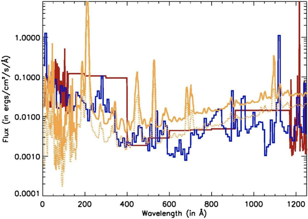
Fig. 7. SED in the young (yellow dotted), current Sun (yellow solid) as compared to the X5.5 solar flare (blue) and M dwarf (red) (Airapetian et al., Reference Airapetian, Glocer, Khazanov, Loyd, ROP, France, K, Sojka, J, Danchi, WC and Liemohn, MW2017a).
Theoretical models of XUV emission from planet hosting stars are based by multi-dimensional MHD simulations of stellar coronae and winds driven by the energy flux generated in the chromosphere constrained by FUV emission line fluxes and ground-based spectropolarimetric observation enabled reconstruction of stellar surface magnetic fields are in early phase of development. The first data-driven three-dimensional (3D) MHD model of global corona of a young solar twin star, k 1Ceti, has recently been developed by Airapetian et al. (Reference Airapetian, Jin, Lugtinger, Danchi, van der Holst and Manchester2019b). Two different techniques are mostly used to reconstruct stellar magnetism, namely the Zeeman broadening technique (ZB, Johns-Krull, Reference Johns-Krull2007) and the Zeeman Doppler imaging technique (ZDI, Donati and Brown, Reference Donati and Brown1997). The ZB technique measures Zeeman-induced line broadening of unpolarized light (Stokes I). This technique is sensitive to the total (to large- and small-scale), unsigned surface field. The ZDI technique recovers information about the large-scale magnetic field (its intensity and orientation) from a series of circularly polarized spectra (Stokes V signatures). These techniques have their limitations. While ZB provides a measurement of the total field, it does not provide a measurement of the field polarity. On the other hand, while ZDI provides measurement of the field polarity, it does not have access to small-scale fields. For this reason, these techniques are complementary to each other (see, e.g. Vidotto et al., Reference Vidotto, Gregory, Jardine, Donati, Petit, Morin, Folsom, Bouvier, Cameron, Hussain, Marsden, Waite, Fares, Jeffers and do Nascimento2014).
Using ZDI magnetic maps, Vidotto et al. (Reference Vidotto, Gregory, Jardine, Donati, Petit, Morin, Folsom, Bouvier, Cameron, Hussain, Marsden, Waite, Fares, Jeffers and do Nascimento2014) demonstrated that the average, unsigned large-scale magnetic field of solar like stars decay with age and with rotation (see also Petit et al., Reference Petit, Dintrans, Solanki, Donati, Aurière, Lignières, Morin, Paletou, Ramirez Velez, Catala and Fares2008; Folsom et al., Reference Folsom, Bouvier, Petit, Lèbre, Amard, Palacios, Morin, Donati and Vidotto2018) as, respectively,


These empirical trends provide important constraints on the evolution of the large-scale magnetism of cool stars. In particular, the magnetism–age relation (see Fig. 8) presents a similar power dependence empirically identified in the seminal work of Skumanich (Reference Skumanich1972) and the magnetism–rotation relation suggests that a linear dynamo of the type B ~ 1/P rot is in operation in solar-like stars. These empirical relations contain significant spread partially caused due to magnetic-field evolution on years, and sometimes only months (see Fig. 8).
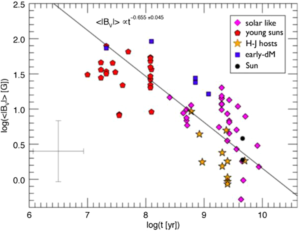
Fig. 8. Empirical relation between the unsigned average stellar magnetic field (derived using the ZDI technique) and age. Figure from Vidotto et al. (Reference Vidotto, Gregory, Jardine, Donati, Petit, Morin, Folsom, Bouvier, Cameron, Hussain, Marsden, Waite, Fares, Jeffers and do Nascimento2014).
Given that ZDI allows one to obtain the topology of the surface magnetic field, See et al. (Reference See, Jardine, Vidotto, Donati, Folsom, Boro Saikia, Bouvier, Fares, Gregory, Hussain, Jeffers, Marsden, Morin, Moutou, do Nascimento, Petit, Rosén and Waite2015) investigated the energy contained in the poloidal and toroidal components of the stellar surface field. They found that the energy in these components are correlated with solar-type stars more massive than 0.5 M⊙ having 〈B tor2〉 ~ 〈B pol2〉1.25±0.06.
Winds from active stars
Stellar winds represent an extension of global stellar corona into the IP space and are fundamental property of F–M dwarf stars. Stellar coronal winds are weak and no reliable detection of a wind from another star other than the Sun was reported. The empirical method of detection of stellar wind relies on the observations of HI Ly-α absorption from the stellar astrosphere forming due to the wind interaction with the surrounding interstellar medium (Wood, Reference Wood2018). The mass loss rates from young GK dwarfs are well correlated with X-ray coronal flux as $\dot M \propto F_{\rm X}^{1.29}$ reaching the maximum rates of 100 times of the current Sun's rate. However, this relation fails for stars with the greater X-ray flux suggesting the saturation of surface magnetic flux (see section ‘Origin and patterns of solar-magnetic activity: global solar corona’).
Recent measurements of surface magnetic fields and X-ray properties of the coronae from solar-type stars paved a way for inputs to heliophysics based multi-dimensional models of the stellar coronae and winds using ‘Star-As-The-Sun’ approach. This approach suggests the availability of stellar inputs and boundary conditions to be used for heliophysics MHD code. The first MHD wind models from young solar-type stars resembling our Sun in its infancy were developed by Sterenborg et al. (Reference Sterenborg, Cohen, Drake and Gombosi2011); Airapetian and Usmanov (Reference Airapetian and Usmanov2016); do Nascimento et al. (Reference do Nascimento, Vidotto, Petit, Folsom, Castro, Marsden, Morin, de Mello GF, Meibom, Jeffers, Guinan and Ribas2016) and Ó Fionnagáin et al. (Reference Ó Fionnagáin, Vidotto, Petit, Folsom, Jeffers, Marsden, Morin and do Nascimento2018). Specifically, the young Sun's wind speed at 1 AU was twice as fast, five times hotter with the mass loss rate of >50 times greater as compared to the current solar-wind properties (see Fig. 9).

Fig. 9. The model and empirical mass loss rates shown as the shadow region (Wood et al., Reference Wood, Müller, Zank, Linsky and Redfield2005) from the evolving Sun. Red, blue and green stars show the model mass loss rates for the 0.7, 2.2 and 4.65 Gyr old Sun (Airapetian and Usmanov, Reference Airapetian and Usmanov2016).
The young Sun's wind model was recently extended to describe the formation of global solar corona by incorporating the observationally derived stellar magnetograms and the chromospheric parameters of the best-known young Sun's proxy, k 1Cet, into the data-driven 3D MHD thermodynamic model (Airapetian et al., Reference Airapetian, Jin, Lugtinger, Danchi, van der Holst and Manchester2019b). Figure 10 shows the drastic change in the topology of global magnetic field of the star in 11 months (2012.9 (left) and 2013.8 (right)). If the shape of global stellar corona in the left panel resemble a dipole-like magnetic field, global coronal field tilts at 45° and becomes complex. The model predicts that the variation of X-ray flux by a factor of 2 over 11 months. The coordinated spectropolarimetric observations that provide stellar magnetic field with TESS, HST and X-ray observations (XMM-Newton and NICER mission) are currently in place to provide epoch specific model inputs and outputs that are required to check the model predictions. Recent spectropolarimetric observations of another active star, K dwarf, 61 Cyg A, show that the star's magnetic field has undergone full dipole flip during the magnetic cycle (Boro Saikia et al., Reference Saikia S, Lueftinger, Jeffers, Folsom, See, Petit, Marsden, Vidotto, Morin, Reiners and Guedel2018). Such data-driven models are required in order to characterize the range of variations of ionizing radiation fluxes and their timescale in order to assess the impact of the stellar high-energy radiation onto habitability of exoplanets.
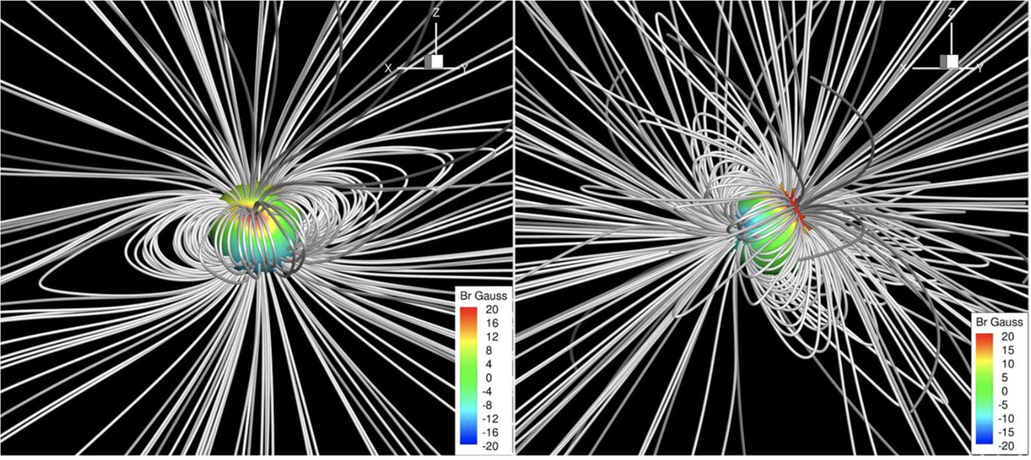
Fig. 10. The evolution of the 0.7 Gyr Sun proxy's global magnetic field over the course of 11 months, at 2012.9 (left) and 2013.8 (right) (from Airapetian et al., Reference Airapetian, Jin, Lugtinger, Danchi, van der Holst and Manchester2019b).
Superflares from active stars
Recent observations of stars of F, G, K and M spectral types in X-ray, UV and optical bands provide evidence of stellar flares with energy release 10–10 000 times larger than that of the largest solar flare ever observed on the Sun and referred to as superflares (Schaefer et al., Reference Schaefer, King and Deliyannis2000; Walkowicz et al., Reference Walkowicz, Basri, Batalha, Gilliland, Jenkins, Borucki, Koch, Caldwell, Dupree, Latham, Meibom, Howell, Brown and Bryson2011; Zhou et al., Reference Zhou, Li and Wang2010; Maehara et al., Reference Maehara, Shibayama, Notsu, Notsu, Nagao, Kusaba, Honda, Nogami and Shibata2012, Reference Maehara, Shibayama, Notsu, Notsu, Honda, Nogami and Shibata2015, Reference Maehara, Notsu, Notsu, Namekata, Honda, Ishii, Nogami and Shibata2017). The energy of the smallest detected solar flare (a nanoflare which was recently detected by Focusing Optics X-ray Solar Imager (FOXSI) mission) is 13 orders of magnitude smaller than the largest stellar superflare from active stars. Many lines of evidence suggest that solar flares are powered by magnetic reconnection of coronal magnetic fields emerging from the solar convective zone into the solar corona (Shibata and Magara, Reference Shibata and Magara2011).
This raises a fundamental question i.e. whether powerful stellar flares on magnetically active stars are also driven by magnetic energy release? If they are, then can we extrapolate statistics of white-light solar flares and its energy partition into different modes of energy release (direct heating, non-thermal energy of electrons and ions and kinetic energy of flows) to 5 orders of magnitude? Because our understanding of the nature of solar flares is far from complete, we need to rely on statistical patterns observed for solar and stellar flares. Characterization of the frequency of occurrence of flares with energy may serve as one of such important discriminators. The measurements of solar hard X-ray (HXR) bursts obtained by the Solar Maximum Mission (SMM), radio and optical bands suggest that the frequency of occurrence of flares, dN, within the energy interval E, E + δE follows a power law with flare energy as

with power law index, α, varying between −1.13 and −2 (Crosby et al., Reference Crosby, Aschwanden and Dennis1993). The data suggest that flare energy distribution in the optical band corresponds to α = −1.8. This can be directly compared to recent optical observations by the Kepler mission of thousands of white-light flares on hundreds of G, K and M dwarfs (Maehara et al., Reference Maehara, Shibayama, Notsu, Notsu, Nagao, Kusaba, Honda, Nogami and Shibata2012). The power-law index for superflares from both short- and long-cadence data, band corresponds to α = −1.5 ± 0.1 for flare energies from 4 × 1033 to 1036 erg (Maehara et al., Reference Maehara, Shibayama, Notsu, Notsu, Honda, Nogami and Shibata2015).
Figure 11 shows the frequency distribution for a range of flare processes: from the smallest solar flares to the most powerful stellar superflares. Filled circles indicate the frequency distribution of superflares on Sun-like stars (G-type main sequence stars with P rot > 10 days and 5800 < T eff < 6300 K) derived from short-cadence data. Horizontal error bars represent the range of each energy bin. Bold solid line represents the power-law frequency distribution of superflares on Sun-like stars taken from (Shibayama et al., Reference Shibayama, Maehara, Notsu, Notsu, Nagao, Honda, Ishii, Nogami and Shibata2013). Dashed lines indicate the power-law frequency distribution of solar flares observed in HXR (Crosby et al., Reference Crosby, Aschwanden and Dennis1993), soft X-ray (Shimizu, Reference Shimizu1995) and EUV bands. Frequency distributions of superflares on Sun-like stars and solar flares are roughly on the same power-law line with an index of α = −1.8 (thin solid line) for the wide energy range between 1024 and 1035 erg. Shibayama et al. (Reference Shibayama, Maehara, Notsu, Notsu, Nagao, Honda, Ishii, Nogami and Shibata2013) found that superflares from young (0.7 Gyr) solar-like stars with the energy of 1034 erg occur at the rate of 0.1 event per day, which suggests that the frequency of superflares with energies ~1033 erg (see Fig. 11) is ~10 events per day. The event of the comparable energy was observed on 1–2 September 1859 by British astronomers Richard Carrington (Carrington, Reference Carrington1859) and Richard Hodgson (Hodgson, Reference Hodgson1859) and was coined as the Carrington event. Recent studies suggest that our Sun had produced powerful flares associated with CMEs with the energy at least 3–10 times stronger than the Carrington event. Possible solar superflare events could be associated with extreme solar proton events (SPEs) that produce cosmogenic radionuclides including the enhanced content of carbon-14, 14C, detected in tree rings, beryllium-10, 10Be and chlorine-36, 36Cl, measured in both Arctic and Antarctic ice cores (Mekhaldi et al., Reference Mekhaldi, Muscheler, Adolphi, Aldahan, Beer, McConnell, Possnert, Sigl, Svensson, Synal, Welten and Woodruff2015). These data suggest that solar superflares events were accompanied with hard energy SEP protons occurred in AD 774 to 775, AD 993 to 994 and 660 BC (Miyake et al., Reference Miyake, Nagaya, Masuda and Nakamura2012, Reference Miyake, Masuda and Nakamura2013; O'Hare et al., Reference O'Hare, Mekhaldi, Adolphi, Raisbeck, Aldahan, Anderberg, Beer, Christl, Fahrni, Synal, Park, Possnert, Southon, Bard, Aster and Muscheler2019). The proton fluence associated with such powerful events would be equivalent to solar flares with the energy of ~1034 erg. The occurrence frequency of these events (two events in 220 years) is roughly comparable to the average occurrence frequency of superflares on Sun-like stars with the energy of 1033–1034 erg.
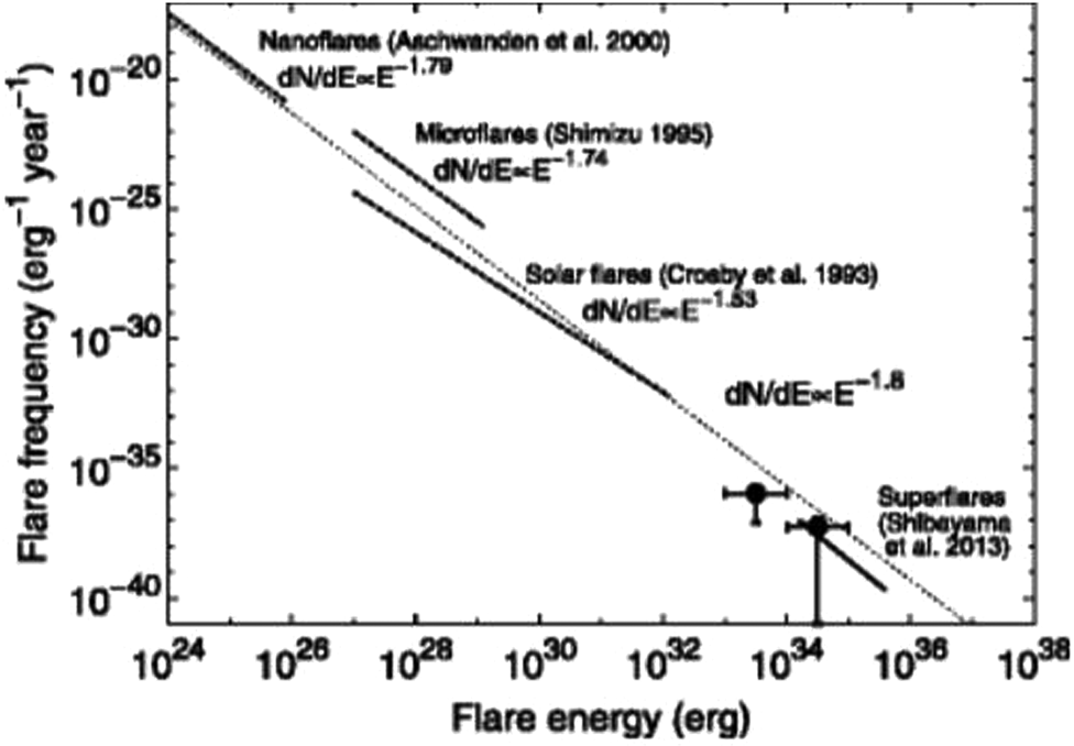
Fig. 11. The power-law distribution of frequency of occurrence of solar and stellar flares.
As the Sun evolved to the current age, its flare frequency was reduced dramatically to one event per 70, 500 and 4000 years for the flare bolometric energies of 1033, 1034 and 1035 erg, respectively. Also, data suggest that the frequency of superflares strongly depends on the rotation period, P rot (Notsu et al., Reference Notsu, Shibayama, Maehara, Notsu, Nagao, Honda, Ishii, Nogami and Shibata2013; Maehara et al., Reference Maehara, Shibayama, Notsu, Notsu, Honda, Nogami and Shibata2015; Davenport, Reference Davenport2016). These frequencies are lower than the upper limits derived from radionuclides in lunar samples (Schrijver et al., Reference Schrijver, Kauristie, Aylward, Denardini, Gibson, Glover, Gopalswamy, Grande, Hapgood, Heynderickx, Jakowski, Kalegaev, Lapenta, Linker, Liu, Mandrini, Mann, Nagatsuma, Nandy, Obara, Paul O'Brien, Onsager, Opgenoorth, Terkildsen, Valladares and Vilmer2015).
The frequency of stellar superflares also correlates with the effective temperatures of the star. Kepler data indicate that main sequence stars with lower temperature exhibit more frequent superflares. The frequency of superflares on K- and early M-type stars (T eff = 4000–5000 K) is roughly 1 order of magnitude higher than that on G-type stars (e.g. Candelaresi et al., Reference Candelaresi, Hillier, Maehara, Brandenburg and Shibata2014).
As described above, the flare frequency depends on the rotation period. On the other hand, Kepler data suggest that the bolometric energy of the largest superflare on solar-type stars does not depend on the rotation period (e.g. Maehara et al., Reference Maehara, Shibayama, Notsu, Notsu, Nagao, Kusaba, Honda, Nogami and Shibata2012; Notsu et al., Reference Notsu, Shibayama, Maehara, Notsu, Nagao, Honda, Ishii, Nogami and Shibata2013). This implies that the slowly-rotating solar-type stars could exhibit superflares with the energy of 1034–1035 erg. Most of superflare stars show periodic brightness variations with the amplitude of ~1% due to the rotation of the star which suggest that the stars showing superflares may have large starspots on their surface. According to Shibata et al. (Reference Shibata, Isobe, Hillier, Choudhuri, Maehara, Ishii, Shibayama, Notsu, Notsu, Nagao, Honda and Nogami2013), the energy of the largest superflares is roughly proportional to A spot3/2 (A spot is the starspot area), and large starspots with the area of >1% of the solar hemisphere (>3 × 1020 cm2) would be necessary to produce superflares with the energy of ≥1034 erg.
Existence of starspots on Kepler superflare stars are also supported from the follow-up spectroscopic observations (Notsu et al., Reference Notsu, Shibayama, Maehara, Notsu, Nagao, Honda, Ishii, Nogami and Shibata2013; Karoff et al., Reference Karoff, Knuden, De Cat, Bonanno, Fogtmann-Schulz, Fu, Frasca, Inceoglu, Olsen, Zhang, Hou, Wang, Shi and Zhang2016). A recent statistical analysis of starspots based on Kepler data performed suggests that the magnetic activity pattern in terms of the frequency-energy distribution of solar flares is consistent with superflares detected on more active solar-like stars, which implies that the same magnetically driven physical processes of the energy release within coronal active regions are responsible for the origin of solar and stellar flares (Maehara et al., Reference Maehara, Notsu, Notsu, Namekata, Honda, Ishii, Nogami and Shibata2017). Recent estimates of lifetimes and emergence/decay rates of large starspots on young solar-type stars suggest that sunspots and large starspots share the same underlying processes (Namekata et al., Reference Namekata, Maehara, Notsu, Toriumi, Hayakawa, Ikuta, Notsu, Honda, Nogami and Shibata2018).
Coronal mass ejections from active stars
As discussed in the section ‘Origin and patterns of solar-magnetic activity: transient events’, large solar flares are associated with powerful CMEs. Because eruptive events on solar-types stars are also driven by magnetic-field energy, this begs the important question as to whether we can use correlations between X-ray flare fluxes and CME parameters to derive the properties of stellar CMEs, estimate their rates of occurrence and derive their observational signatures. The sub-section ‘MHD models of stellar CMEs’ discusses recent efforts in modelling CMEs on other stars from first principles and the model predictions of their properties. The sub-section ‘Search for stellar CMEs’ presents the summary of recent searches of CMEs and its methodology.
MHD models of stellar CMEs
Sudden eruptions on the Sun and solar-type stars occur due to the rapid release of free magnetic energy stored in the sheared and/or twisted strong fields typically associated with sunspots and active regions (e.g. Fletcher et al., Reference Fletcher, Dennis, Hudson, Krucker, Phillips, Veronig, Battaglia, Bone, Caspi, Chen, Gallagher, Grigis, Ji, Liu, Milligan and Temmer2011; Shibata and Magara, Reference Shibata and Magara2011; Kazachenko et al., Reference Kazachenko, Canfield, Longcope and Qiu2012; Janvier et al., Reference Janvier, Aulanier and Démoulin2015). Large flares are often accompanied by CMEs (Gopalswamy et al., Reference Gopalswamy, Yashiro, Liu, Michalek, Vourlidas, Kaiser and Howard2005). Regardless of the specific details of the ideal or resistive instabilities that initiate the catastrophic, run-away eruption of CMEs, the relationship between the eruptive flare and its resulting CME is well understood (Forbes, Reference Forbes2000; Zhang and Dere, Reference Zhang and Dere2006; Lynch et al., Reference Lynch, Masson, Li, DeVore, Luhmann, Antiochos and Fisher2016; Welsch, Reference Welsch2018; Green et al., Reference Green, Török, Vršnak, Manchester and Veronig2018).
One such model for the initiation and launching of solar CMEs into the corona in global and local active region environments is the magnetic breakout model (Antiochos et al., Reference Antiochos, DeVore and Klimchuk1999; DeVore and Antiochos, Reference DeVore and Antiochos2008; Lynch et al., Reference Lynch, Antiochos, DeVore, Luhmann and Zurbuchen2008, Reference Lynch, Antiochos, Li, Luhmann and DeVore2009; Karpen et al., Reference Karpen, Antiochos and DeVore2012; Masson et al., Reference Masson, Antiochos and DeVore2013). Lynch et al. (Reference Lynch, Masson, Li, DeVore, Luhmann, Antiochos and Fisher2016) have demonstrated that even in bipolar streamer distributions, the overlying, restraining closed flux is removed in a breakout-like way through an opening into the solar wind, thus enabling the eruption of low-lying energized flux. Therefore, the evolution and interaction between the low-lying energized and overlying restraining fields are extremely important aspects of modelling eruption processes in solar and stellar coronae to correctly estimate the CME EJ properties and energetics. Figure 12 illustrates recent ARMS 3D simulation results by Lynch et al. of a massive halo-type (width of 360°, see Fig. 12) energetic CME eruption based on the observationally derived k 1Cet magnetogram. The entire stellar streamer-belt visible on this figure is energized via radial field-preserving shearing flows and the eruption releases ~7 × 1033 erg of magnetic free energy in ~10 h (Lynch et al., Reference Lynch, Airapetian, Kazachenko, Lüftinger, DeVore and Abbett2019). Magnetic reconnection during the stellar flare creates the twisted flux rope structure of the EJ and the ~2000 km s−1 eruption creates a CME-driven strongly magnetized shock.
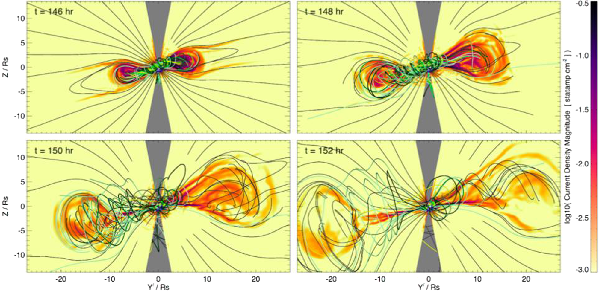
Fig. 12. ARMS 3D simulation of a massive (Carrington scale) stellar coronal eruption initiated from the k 1Cet magnetogram. The contour planes show current density magnitude in the erupting flux rope.
The maximum increase in total kinetic energy during the eruption was ~2.8 × 1033 erg – on the order of the 1859 Carrington flare event. The meridional planes plot the logarithmic current density magnitude showing the circular cross-section the CME (Vourlidas et al., Reference Vourlidas, Lynch, Howard and Li2013) and representative magnetic-field lines illustrate 3D flux rope structure.
A CME-initiation process from an active region (compact CMEs) suggests that a solar-like star with the large-scale dipolar magnetic field of 75 G would confine impulsive coronal eruptions with energies less than 3 × 1032 erg. Thus, only Carrington-type flare eruptions can eject compact CMEs from these stars. These results also imply that strong (~600–1000 G) dipole fields on young active M dwarfs would confine CMEs with E < 3 × 1034 erg, and thus, should occur at much lower (at least 10 000 times) frequency that the flare frequencies that are typically ~1 event per hour.
Search for stellar CMEs
If we apply the empirical relationships solar-energetic flares and associated CMEs (see section ‘Origin and patterns of solar-magnetic activity: transient events’), then stellar superflares should be associated with fast and massive CMEs from magnetically active stars. Can we observationally detect these large stellar CMEs? The three major observational techniques for detecting the signatures of stellar CMEs include (a) type-II radio bursts; (b) Doppler shifts in UV/optical lines and (c) continuous absorption in the X-ray spectrum. Type-II radio bursts occur at the low frequency of <30 MHz. Within few minutes the burst frequency shifts to <1 MHz. The emission below 8–15 MHz cannot be detected from the Earth due to the reflection from the terrestrial ionosphere (Davies, Reference Davies1969). Also, high-velocity outflows generated during powerful stellar eruptions could also be signatures of CMEs. A detection of blue-shifted hydrogen and Ca II chromospheric lines from the spectrum of the young M dwarf star, AD Leo, during a powerful superflare event (with the energy of >1034 erg) could be possibly associated with the massive CMW with the speed up to 5800 km s−1 (Houdebine et al., Reference Houdebine, Foing and Rodono1990). Another signature of stellar CMEs could be associated with the excess amount of absorption of X-ray emission as for example for observed early in the flare from UX Ari (Franciosini et al., Reference Franciosini, Pallavicini and Tagliaferri2001). This absorption requires five times greater column density in neutral hydrogen that attributable to the interstellar medium on the line of sight. Favata and Schmitt (Reference Favata and Schmitt1999) discussed X-ray absorption observed during a superflare from Algol star as a signature of a giant CME. Recently, Moschou et al. (Reference Moschou, Drake, Cohen, Alvarado-Gomez and Garraffo2018) have extended their suggestion to a stellar CME model that can fit the statistical correlations of CME mass with X-ray flare flux. The aforementioned and other possible observational signatures of stellar flares and CMEs are summarized in Table 1.
Table 1. Comparison of observational signatures used to study flares and CMEs on the Sun and in aggregates across other stars
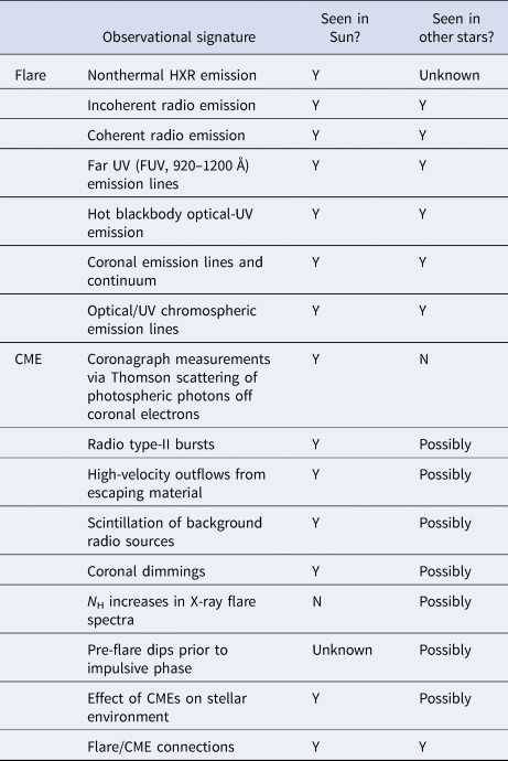
It is evident that there is significant overlap between observational signatures of flares on the Sun and other stars, even if on closer examination the specific bandpasses and observing methods differ (e.g. spatially and temporally resolved solar observations versus spatially integrated temporal stellar observations). Osten (Reference Osten, Schrijver, Bagenal and Sojka2016) discusses the observational perspective on stellar flares and what is known about stellar flaring events throughout the age of the Solar system. The comparison for CMEs shows significantly less overlap; this is due primarily to the much lower contrast of the ejected material compared to the stellar disc, and the need to disentangle any CME-related emission from flare-related emission in order to attribute a signature entirely to a CME. To date, while there have been suggestions of ejections of CMEs in solar-type stars, these have generally been attributed to specific circumstances, such that the wider applicability is unknown. Osten and Wolk (Reference Osten, Wolk, Nandi, Valio and Petit2017) described the framework for finding and interpreting stellar CMEs, including a discussion of the observational signatures listed in Table 1.
As discussed in the previous section, given that only energetic CMEs can be ejected into the astrosphere, the frequency of CMEs on magnetically active stars should be reduced the by at least 1–2 orders of magnitude. Also, the expected radio frequency from shocks associated with energetic CMEs and superflares from magnetically active stars should be in the order of 10 MHz or lower. This suggests that extended low-frequency observations are required to hunt for elusive stellar CMEs.
Impact of space weather effects on modern Earth, Venus and Mars
Distinguishing the different evolutionary pathways of Earth and its rocky neighbours, as well as for Earth-like planets are central tasks in (exo)planetary science. Much is to be learned by comparing the response of a rocky planet which features a magnetosphere (the Earth) to changes in stellar output compared with the responses of our weakly magnetized neighbouring planets Venus and Mars (Brain et al., Reference Brain, Bagenal, Ma, Nilsson and Stenberg Wieser2017). Did Venus’ climate evolve via a runaway greenhouse from earlier, potentially habitable conditions (Way et al., Reference Way, Del Genio, Kiang, Sohl, Grinspoon, Aleinov and Clune2016) into its current extreme state (Bullock and Grinspoon, Reference Bullock and Grinspoon2001)? What role the Sun played in its climate evolution (e.g. Lammer et al., Reference Lammer, Güdel, Kulikov, Ribas, Zaqarashvili, Khodachenko, Kislyakova, Gröller, Odert, Leitzinger, Fichtinger, Krauss, Hausleitner, Holmström, Sanz-Forcada, Lichtenegger, Hanslmeier, Shematovich, Bisikalo, Rauer and Fridlund2012)? Is Venus a magma ocean planet preserved from its early phase (Hamano et al., Reference Hamano, Abe and Genda2013)? How and to what extent escape processes driven by stellar output drove atmospheric loss of the Martian atmosphere into its current cold, dry, dusty state is a key theme in Martian science (Jakosky and Phillips, Reference Jakosky and Phillips2001)?
Chemical responses of planetary atmospheres to SW can be broadly split into two mechanisms – firstly due to enhanced radiation (e.g. EUV) which enhances e.g. photolytic destruction and secondly due to interaction of gas-phase species with high-energy particles. Space plasma interaction responses can similarly be classified as either atmospheric ion erosion or sputtering of neutral atmosphere by the energized ions that are not on escape trajectories but instead deposit their gained energies into the upper atmosphere. But first it is useful to briefly consider the situation at the Earth for comparisons.
Modern Earth
Our planet, like all the other terrestrial planets in our Solar system, is exposed to the XUV and particle emissions from the quiescent and active Sun. The latter includes the solar-wind plasma with its embedded magnetic fields. The extremes of these external influences occur in the forms of solar flares, CME-driven plasma and magnetic-field enhancements proceeded by shocks, and the related SEPs. In addition, galactic cosmic rays (GCRs) diffuse into the inner heliosphere and into the planetary atmospheres. Each of these has specific atmospheric (and related surface) influences, with those affecting Earth the most potentially consequential for both our technological society and the biosphere. Such effects, which can also have evolutionary timescale influences of importance, can generally be classified into two main categories: atmospheric erosion or loss to space that can become significant on long timescales, and atmospheric chemistry alterations, which can have both long- and short-term impacts.
Space weather drivers of ionospheric outflows
The contemporary flux of outflowing ions at high latitudes at the Earth is a combination of a light ion (hydrogen and helium ion) dominated ‘polar wind’ and heavier ion outflows composed mainly of oxygen ions associated with auroral activity (Yau and André, Reference Yau and André1997) that is of most interest here. The estimated integrated oxygen ion outflows are of the order of 1024 s−1 for low geomagnetic activity and 1026 s−1 for high activity. For the Earth, the solar wind does not interact directly with the ionosphere because of the presence of a planetary scale magnetic field. Nevertheless, the solar wind does interact with the Earth's magnetosphere, primarily through magnetic-field reconnection. This allows solar-wind momentum and energy to be coupled into the magnetosphere, and affect the high latitude ionosphere, mainly in the auroral zone and cusp region (e.g. see Moore et al., Reference Moore, Fok, Delcourt, Slinker and Fedder2010 and references therein). The latter is the more direct point of entry for solar-wind-related energy fluxes, be they particle or electromagnetic energy fluxes. This was explored by Strangeway et al. (Reference Strangeway, Ergun, Su, Carlson and Elphic2005) using data from the Fast Auroral Snapshot (FAST) Small Explorer. FAST acquired data from a high inclination elliptical orbit with apogee around 4000 km altitude. Strangeway et al. (Reference Strangeway, Ergun, Su, Carlson and Elphic2005) derived scaling laws that related Poynting flux (electromagnetic energy flux) and precipitating auroral electron fluxes (particle energy) to ion outflows. This analysis was extended by Brambles et al. (Reference Brambles, Lotko, Zhang, Wiltberger, Lyon and Strangeway2011) to include the effects of Alfvén waves, which are an additional source of electromagnetic energy flux. The connections explored by Strangeway et al. (Reference Strangeway, Ergun, Su, Carlson and Elphic2005) and Brambles et al. (Reference Brambles, Lotko, Zhang, Wiltberger, Lyon and Strangeway2011) are illustrated in Fig. 13. Moore and Horwitz (Reference Moore and Horwitz2007) also explored these connections with numerical simulations as a means of understanding and interpreting the global picture of the various processes at work that lead to the heavy ion energization and escape.

Fig. 13. Connections between input energy fluxes and outflowing ions as explored by in situ measurements above the ionosphere (after Strangeway et al., Reference Strangeway, Ergun, Su, Carlson and Elphic2005, with the addition of Alfvén waves as an energy source).
The upper part of Fig. 13 shows parameters measured above the ionosphere (in green), as well as the type of connection: correlated (magenta arrows) or possibly causal (open blue arrows). As an example of a possible causal relation, Alfvén waves could contribute to the Poynting flux into the ionosphere (left-hand path) or to enhanced precipitating electron fluxes (right-hand path). It is known that some form of heating is required for upwelling ions to escape (the escape energy for oxygen ions at the Earth is ~10 eV, at least an order of magnitude larger than the temperature of upwelling ions). Since the Poynting flux is carried by field-aligned currents (FACs), it is also possible that the FACs could contribute to heating via a current-driven instability, while the precipitating electrons may also be a source of free energy for wave instabilities.
The lower half of Fig. 13 shows how the incoming energy fluxes can result in outflows. For the left-hand path the electromagnetic energy results in Joule dissipation that heats the ions in the ionosphere, increasing the scale-height, so that more ions up-well to altitudes were waves can heat the ions, allowing them to escape. The right-hand path corresponds to electron precipitation that increases the ionospheric electron temperature. The resultant ambipolar electric field also increases the ionospheric scale height. Moore and Horwitz (Reference Moore and Horwitz2007) explored these connections, using numerical simulations to understand and interpret the global picture of the various processes at work that lead to the heavy ion energization and escape.
Much like the solar-wind interaction with the unmagnetized planets, the ultimate energy source to drive the ionospheric outflows at the Earth is the solar wind. But what is less clear is how efficiently that energy is coupled to the ionosphere. The planetary magnetic field inhibits any direct interaction with the ionosphere, but also makes the planetary obstacle much larger, with an effective radius of the order 10 Earth radii. At the same time, the amount of energy available to drive outflows depends on the highly variable reconnection efficiency. The Earth's magnetic field also results in any energy from the solar wind being mainly directed to the polar ionosphere. Whether or not the outflowing ions ultimately escape the magnetosphere depends on their transport through the magnetotail lobes. The ions could escape downtail, or be convected into the plasmasheet where they are then transported sunwards. Kistler et al. (Reference Kistler, Galvin, Popecki, Simunac, Farrugia, Moebius, Lee, Blush, Bochsler, Wurz, Klecker, Wimmer-Schweingruber, Opitz, Sauvaud, Thompson and Russell2010) have reported escaping fluxes of the order 1024 s−1 for downtail, and they argue that most of the outflowing ions are transported to the plasmasheet. But even then some of the ions could escape through transport to the dayside magnetopause. Fuselier et al. (Reference Fuselier, Burch, Mukherjee, Genestreti, Vines, Gomez, Goldstein, Trattner, Petrinec, Lavraud and Strangeway2017) have shown that ions of ionospheric origin are transported to the dayside magnetopause, although the mass density of these ions is a small fraction of the magnetosheath plasma mass density.
The question for planetary atmospheric erosion through ionospheric escape is how do the ionospheric rates for the magnetized and unmagnetized planets vary as a function of the drivers, such as the solar-wind dynamic pressure and solar EUV, and what role does a planetary scale magnetic field have in enhancing or inhibiting ionospheric outflow and loss? It may be purely coincidence that planetary outflow rates for Venus, the Earth and Mars are of the same order of magnitude. The answer to this question requires developing a detailed understanding of the various processes involved, and including such processes in models that allow us to explore parameter regimes including those corresponding to the early Solar system (see sections ‘Atmospheric escape: effect of stellar XUV flux’ and ‘Impact of space weather on atmospheric chemistry of early Earth and Mars’).
Space weather effects on the chemistry of ionosphere–thermosphere system
SEP events represent protons and heavy ions with energies from MeV to tens of MeV for gradual events lasting for days and from tens of MeV to several hundred MeV for impulsive events lasting for hours. These types of events are often associated with large solar flares and CMEs. At Earth, similarly energetic particles occupy the radiation belts, which are perturbed (both enhanced and depleted) as a part of the related geomagnetic activity. The Energetic Electron Precipitation (EEP) events are divided into three categories based on their origin of precipitation and energy: (a) low-energy electrons (LEE, <30 KeV), (b) medium-energy electrons (MEE, 30–300 KeV) and (c) high-energy electrons (HEE, 300 KeV to several MeV). The LEEs reside in the magnetosphere, whereas MEE and HEE are trapped in the outer Van Allen radiation belt, from where they precipitate into the atmosphere during GM and sub-storms (Sinnhuber et al., Reference Sinnhuber, Nieder and Wieters2012; Andersson et al., Reference Andersson, Verronen, Rodger, Clilverd and Seppälä2014). The LEEs affect the atmospheric ion chemistry >90 km, the MEEs affect the atmospheric ion chemistry between 70 and 90 km (Egorova et al., Reference Egorova, Rozanov, Ozolin, Shapiro, Calisto, Peter and Schmutz2011), and the HEEs affect atmospheric chemistry <70 km at middle and high latitudes (Mironova et al., Reference Mironova, Aplin, Arnold, Bazilevskaya, Harrison, Krivolutsky, Nicoll, Rozanov, Turunen and Usoskin2015). Finally, the GCRs originate from outside of our Solar system and consist of high-energy protons with energies ranging from ~1 MeV up to ~1015 MeV (Mironova et al., Reference Mironova, Aplin, Arnold, Bazilevskaya, Harrison, Krivolutsky, Nicoll, Rozanov, Turunen and Usoskin2015). They are the main source of ionization between 3 and 40 km. Due to geomagnetic-field cutoffs that reduce the access of the lower energy GCRs to low-to-mid latitudes, the maximum ionization occurs at around 10 km at the poles and gradually decreases towards the equator (Usoskin et al., Reference Usoskin, Mironova, Korte and Kovaltsov2010). These cutoffs also affect the access of SEPs to the atmosphere. The ionization rate by GCRs is about three orders of magnitude compared to the rest of the EPP events.
EPP events affect the middle-to-upper atmosphere at middle-to-high latitudes by modulating the local atmospheric ion chemistry by increasing the local ionization rate (Wissing and Kallenrode, Reference Wissing and Kallenrode2009). EPPs produce odd hydrogen (HOx = H, OH, HO2), odd nitrogen (NOx = N, NO, NO2) as well as chlorine compounds, which destroy the upper stratospheric and mesospheric ozone (O3) through a series of catalytic chemical reactions. These processes have been extensively studied using observations, theoretical approaches and modelling (e.g. Rusch et al., Reference Rusch, Gérard, Solomon, Crutzen and Reid1981; Solomon et al., Reference Solomon, Rusch, Gérard, Reid and Crutzen1981; Jackman et al., Reference Jackman, DeLand, Labow, Fleming, Weisenstein, Ko, Sinnhuber and Russell2005, Reference Jackman, Deland, Labow, Fleming and López-Puertas2006, Reference Jackman, Marsh, Vitt, Roble, Randall, Bernath, Funke, López-Puertas, Versick, Stiller, Tylka and Fleming2011; Seppälä et al., Reference Seppälä, Verronen, Sofieva, Tamminen, Kyrölä, Rodger and Clilverd2006; Verronen et al., Reference Verronen, Seppala, Kyrola, Tamminen, Pickett and Turunen2006, Reference Verronen, Rodger, Clilverd, Pickett and Turunen2007, Reference Verronen, Rodger, Clilverd and Wang2011; Damiani et al., Reference Damiani, Storini, Laurenza and Rafanelli2008, Reference Damiani, Storini, Rafanelli and Diego2010; Verkhoglyadova et al., Reference Verkhoglyadova, Wang, Mlynczak, Hunt and Zank2015, Reference Verkhoglyadova, Wissing, Wang, Kallenrode and Zank2016). The lifecycle of HOx is very short (minutes to hours) in the middle atmosphere compared to the NOx lifecycle (months to years). This has further repercussions on the Earth's thermal properties that in turn influence global circulation properties, as we detail below.
In the mesosphere, below 80 km, HOx species can be formed through positively charged O2+ ions that are produced during EPP. These ions interact with water molecules via O4+ to create heavier hydrated O (H2O) ions, which eventually recombine with an electron to convert one water molecule into two odd hydrogen species (OH and H) (Rusch et al., Reference Rusch, Gérard, Solomon, Crutzen and Reid1981) that destroy O3 via: OH + O3 → HO2 + O2. Aside from ion reactions, HOx compounds are also produced via water vapour photolysis (H2O + hv → H + HO) and oxidation (H2O + O(1D) → 2OH). Dissociation and dissociative ionization of N2 during EPP events, also produce NOx species via a series of ion chemistry reactions. Firstly: N2+ + O → NO+ + N(2D). The positive NO+ then reacts with an electron to produce ground state nitrogen and atomic oxygen via: NO+ + e− → N(4S) + O, as well as an excited nitrogen atom and molecular oxygen via: NO+ + e− → N(2D) + O, which further produce NOx species via: N(2D) + O2 → NO + O. Mesospheric O3 is primarily destroyed via: NO + O3 → NO2 + O2, although O3 depletion via NOx at mesospheric altitudes is not as effective as via HOx. Contrary to HOx, the longer-lived, mesospherically-produced NOx species can descend into the upper stratosphere (Solomon et al., Reference Solomon, Crutzen and Roble1982; Russell et al., Reference Russell, Solomon, Gordley, Remsberg and Callis1984; Randall et al., Reference Randall, Harvey, Singleton, Bailey, Bernath, Codrescu, Nakajima and Russell2007) through the polar vortex during high latitude winter (in the absence of sunlight, when the NOx lifetime is particularly long), destroying upper stratospheric O3 during spring via: NO + O3 → NO2 + O2. Meteorologically, the depletion of mesospheric O3 and H2O vapour during EPP events reduces the local heating rate that alters the thermal wind balance, which changes the filtering of mesospheric gravity waves. This causes weaker air ascent and a reduced adiabatic cooling. Evidently, EPP events influence the background atmospheric conditions, which are directly related to numerous atmospheric phenomena such as, mesospheric cloud formation (during summer solstice), circulation and dynamics.
In the upper stratosphere, only very high-energy EPP events directly produce HOx and NOx species to catalytically destroy O3. In the middle and lower stratosphere, where direct SEP production of HOx and NOx species is rare, the primary source of O3 depletion proceeds mainly via NOx species that are dynamically transported downwards from the mesosphere lower thermosphere region. The barrier to mixing at the edge of the polar vortex acts as a containment vessel for NOx species. During the season of the polar vortex, cold temperatures favour heterogeneous chemical reactions on the surface of polar stratospheric clouds, which are extremely important in ozone depletion during winter. One of the most important chemical pathways through which ozone is destroyed inside the polar vortex is the liberation of highly reactive chlorine and bromine forms from their reservoir species via: ClONO2 + HCl → Cl2 + HNO3. While chlorine is being released into the atmosphere, the reactive odd nitrogen species (NOx) are locked up as non-reactive HNO3 and cannot deactivate chlorine. Thus, the chlorine is free to destroy ozone at an extremely efficient rate via the Clx catalytic cycles. After the polar vortex starts dissipating at the beginning of spring, in the presence of sunlight, the unreactive nitrogen reservoir species (e.g. HNO3, N2O5) are transformed into NOx which is released into mid and lower latitudes in the stratosphere destroying the middle and lower stratospheric O3 via the catalytic NOx cycles. The World Meterological Organization (WMO) (2014) assessment provides an in-depth overview of processes affecting ozone in Earth's atmosphere. Since O3 regulates the vertical thermal structure of the stratosphere globally, fluctuations in its concentration induce temperature gradients, which alter the zonal, meridional and vertical winds that drive global circulation and dynamics. Now that we have established the link between EPP events and the physical–chemical pathways through which they could affect atmospheric composition and thermodynamics, we provide a quantitative description of their impact in the terrestrial atmosphere over short and long timescales.
In the mesosphere, satellite observations (Jackman et al., Reference Jackman, DeLand, Labow, Fleming, Weisenstein, Ko, Sinnhuber and Russell2005) and model simulations (Jackman et al., Reference Jackman, Marsh, Vitt, Garcia, Fleming, Labow and Stiller2008) showed >30% decrease in O3 in the polar cap regions (>60° geomagnetic latitude) during the October–November 2003, during strong SPEs. Andersson et al. (Reference Andersson, Verronen, Rodger, Clilverd and Seppälä2014), using satellite observations, showed as high as 90% mesospheric O3 depletion between 60 and 80 km at geomagnetic latitudes 55–65°N/S, during EEP events. In the stratosphere, at high latitudes, modelling studies showed 10–30% O3 reduction due to SPEs (Semeniuk et al., Reference Semeniuk, Fomichev, McConnell, Fu, Melo and Usoskin2011) and EEP events (Rozanov et al., Reference Rozanov, Callis, Schlesinger, Yang, Andronova and Zubov2005). It was found in the late 20th century that O3 was the primary driver of the observed poleward shift of the summer tropospheric jet, which has been linked to changes in tropospheric and surface temperatures, clouds and cloud radiative effects and precipitation at both middle and low latitudes (Previdi and Polvani, Reference Previdi and Polvani2014). Rozanov et al. (Reference Rozanov, Callis, Schlesinger, Yang, Andronova and Zubov2005) found a 2.0 K cooling in the polar middle stratosphere in response to EEP. Calisto et al. (Reference Calisto, Verronen, Rozanov and Peter2012) simulated 3.0 K cooling at 60 km in a possible SPE Carrington-like scenario. EPP events introduce temperature gradients at stratospheric altitudes between the equator and the poles in both hemispheres, which cause acceleration of the meridional winds. To achieve thermal wind balance, the zonal winds accelerate (Limpasuvan et al., Reference Limpasuvan, Hartmann, Thompson, Jeev and Yung2005) by up to 5.0 m s−1 (~20% of the background wind) (Calisto et al., Reference Calisto, Verronen, Rozanov and Peter2012). Stronger zonal winds lead to a more stable polar vortex (Seppälä et al., Reference Seppälä, Lu, Clilverd and Rodger2013) (defined as a large-scale low-pressure area that rotates counter-clockwise in the NH and clockwise in the Southern hemisphere with its base in the upper troposphere extending up to the upper stratosphere). The polar vortex vertically transports HOx and NOx and other chemical species (including greenhouse gases such as, water vapour) and affects the mesospheric (Baumgaertner et al., Reference Baumgaertner, Seppälä, Jöckel and Clilverd2011) and tropospheric (Limpasuvan et al., Reference Limpasuvan, Hartmann, Thompson, Jeev and Yung2005) wind speed patterns.
Although all the studies mentioned above provide an example of how EPP events could influence the terrestrial atmosphere over short-term timescales (days to months), recent studies have started investigating long-term effects of the EPP events. Andersson et al. (Reference Andersson, Verronen, Rodger, Clilverd and Seppälä2014) showed that the integrated effect of short-term events occurring in high frequency leads to long-term effects after observing 34% mesospheric O3 variations over a solar cycle between 2002 and 2012. They identified the continuous LEE precipitation as the missing link in the Sun–Climate system. Whether the longer-term trend of frequency, strength and scale of temporary changes have any impact on atmospheric composition and thermodynamics still remains a question under investigation. Future detailed analyses are required in order to define the coupling processes through which EPP events may influence the terrestrial atmosphere over short and long timescales. Efforts towards this investigation are currently being made by the Intergovernmental Panel on Climate Change (IPCC), which has recognized the possible role of EPPs in global atmospheric variability, and efforts are already underway to include detailed EPP–ozone ion chemistry in the next Coupled Model Intercomparison Project Assessment Report Phase 6 (CMIP6) (Matthes et al., Reference Matthes, Funke, Andersson, Barnard, Beer, Charbonneau, Clilverd, Dudok de Wit, Haberreiter, Hendry, Jackman, Kretzschmar, Kruschke, Kunze, Langematz, Marsh, Maycock, Misios, Rodger, Scaife, Seppälä, Shangguan, Sinnhuber, Tourpali, Usoskin, van de Kamp, Verronen and Versick2017). EPP is a very important factor in the dynamics of Earth's middle atmosphere and is known to induce thermodynamic effects there. We suggest that the particle radiation environment can also influence the dynamics of exoplanetary atmospheres, and ultimately can affect atmospheric escape, hence the evolution of an exoplanetary atmosphere and its long-term variability. There is a strong need to develop pathways to estimate EPP input based on specific stellar environment and extend our knowledge of stellar flares and CME-like eruptions. To estimate EPP effects we need to adapt an atmospheric ionization model to exoplanetary middle atmospheres by incorporating flexible atmospheric chemistry modules suitable for target exoplanets. Establishing such dynamical exoplanetary atmosphere models will aid our understanding of potential biogenic zones and habitability of exoplanets.
For the past 16 years (and counting), NASA's TIMED satellite has been observing Earth's thermosphere and mesosphere, offering unique, unprecedented views of the response of the atmosphere to SW events. Particular interest has been the observations of infrared radiative cooling of the atmosphere by the nitric oxide (NO) and carbon dioxide (CO2) molecules by SABER instrument (Mlynczak, Reference Mlynczak1996, Reference Mlynczak1997; Russell et al., Reference Russell, Mlynczak, Gordley, Tansock and Esplin1999). Shortly after the launch of the TIMED mission in December 2001, SABER observed the first of many GM events in April 2002. Mlynczak et al. (Reference Mlynczak, Martin-Torres, Russell, Beaumont, Jacobson, Kozyra, Lopez-Puertas, Funke, Mertens, Gordley, Picard, Winick, Wintersteiner and Paxton2003, Reference Mlynczak, Martin-Torres, Crowley, Kratz, Funke, Lu, Lopez-Puertas, Russell, Kozyra, Mertens, Sharma, Gordley, Picard, Winick and Paxton2005, Reference Mlynczak, Martin-Torres, Marshall, Thompson, Williams, Turpin, Kratz, Russell, Woods and Gordley2007, Reference Mlynczak, Hunt, Thomas Marshall, Martin-Torres, Mertens, Russell, Remsberg, López-Puertas, Picard, Winick, Wintersteiner, Thompson and Gordley2010, Reference Mlynczak, Hunt, Marshall, Russell, Mertens, Thompson and Gordley2015, Reference Mlynczak, Hunt, Russell, Marshall, Mertens and Thompson2016) demonstrated the role of infrared radiation from NO as a ‘natural thermostat’, effectively serving as the conduit by which GM energy is lost from the atmosphere, allowing it to return to its pre-storm state in a matter of a few days. Mlynczak et al. (Reference Mlynczak, Hunt, Marshall and Russell2018) have shown that for a number of strong storms observed by SABER, approximately 2/3 of the storm energy is radiated in the mid-infrared band by NO molecules, with the other 1/3 radiated by CO2 molecules. The strongest of these infrared, storm-generated signals approach 3 terawatts (globally integrated total). Around younger, more active stars, the total infrared signal may be significantly higher. The infrared signatures of NO, CO2 (and also hydroxyl, OH and O2(1D), electronically excited state of the O2 molecule) are essentially ‘beacons of life’ from exoplanets around young stars that may be readily observed on future space-based and ground-based telescopes (Airapetian et al., Reference Airapetian, Jackman, Mlynczak, Danchi and Hunt2017b). Observations of these infrared emissions confirm the existence of nitrogen, carbon, oxygen (both atomic and molecular) and hydrogen within an exoplanet's atmosphere. The relative abundances of these in an exoplanet could be compared to those on Earth, providing powerful evidence for habitability and the probability of life.
Modern Venus and Mars
One of the striking phenomena observed by spacecraft orbiting Venus and Mars is the apparently continuous escape of atmospheric ions. In particular, oxygen ions, which are often taken to be a proxy for water, are observed with planetary escape rates of the order 1024–1025 s−1 (Brain et al., Reference Brain, Bagenal, Ma, Nilsson and Stenberg Wieser2017), similar to the oxygen ion escape rates for Earth. This is of particular interest because both of these planets lack a global-scale magnetic field, and so the solar wind can interact directly with the planetary upper atmosphere and ionosphere. It has been argued that one of the primary controlling factors for the ion-loss rates in the direct solar-wind–ionosphere interaction is the solar-wind dynamic pressure (Strangeway et al., Reference Strangeway, Russell, Luhmann, Moore, Foster, Barabash and Nilsson2010), and this has been recently verified through MAVEN observations at Mars (Dubinin et al., Reference Dubinin, Fraenz, Pätzold, McFadden, Halekas, DiBraccio, Connerney, Eparvier, Brain, Jakosky, Vaisberg and Zelenyi2017). Another controlling factor appears to be solar EUV flux (e.g. Dubinin et al., Reference Dubinin, Fraenz, Pätzold, McFadden, Halekas, DiBraccio, Connerney, Eparvier, Brain, Jakosky, Vaisberg and Zelenyi2017; Lundin et al., Reference Lundin, Lammer and Ribas2007).
Space weather at modern Venus
Of all other planets, Venus is in many ways the most Earth-like, with comparable surface gravity, a substantial atmosphere, and once orbited within the habitable zone (HZ) of its star (Way et al., Reference Way, Del Genio, Kiang, Sohl, Grinspoon, Aleinov and Clune2016). The inner edge of the HZ moved 4% farther out than Venus's orbital distance at 0.72 AU about 1 Gyr ago. This ignited conditions for a runaway greenhouse on Venus, when the planet lost its oceans within a few tens of millions of years via photodissociation and subsequent escape of hydrogen from the planet at the time when the Sun was 8% less bright than today (Kasting et al., Reference Kasting, Toon and Pollack1988, Reference Kasting, Whitmire and Reynolds1993, Reference Kasting, Kopparapu, Ramirez and Harman2014). This specifies the conditions for the inner edges of HZs for Earth-like planets (Kopparapu et al., Reference Kopparapu, Ramirez, Kasting, Eymet, Robinson, Mahadevan, Terrien, Domagal-Goldman, Meadows and Deshpande2013). However, Venus differs from Earth in another important respect: it has essentially no intrinsic magnetic-dipole field (Smith et al., Reference Smith, Davis, Coleman and Sonett1965; Phillips and McComas, Reference Phillips and McComas1991), and thus the fundamental way it interacts with the Sun is very different from Earth's interaction. Without a magnetic field, the primary obstacle to the solar wind at Venus is the thick, conductive ionosphere. Interplanetary magnetic field (IMF) advecting with the solar wind penetrates the ionosphere and induces a current within, resulting in the generation of an induced magnetosphere (see, e.g. Zhang et al., Reference Zhang, Delva, Baumjohann, Volwerk, Russell, Wei, Wang, Balikhin, Barabash, Auster and Kudela2008 and references therein). This induced magnetic field is an obstacle to the fast solar wind, and thus a bow shock and magnetosheath are generated upstream of the ionosphere (Russell et al., Reference Russell, Elphic and Slavin1979). The induced Venusian magnetosphere is an order of magnitude smaller than the terrestrial intrinsic magnetosphere, with a sub-solar stand-off distance of the bow shock of ~1.5 Venus radii (R V = 6052 km) (Slavin et al., Reference Slavin, Elphic, Russell, Scarf, Wolfe, Mihalov, Intriligator, Brace, Taylor and Daniell1980), as opposed to the ~15 Earth radii (R E = 6371 km) (Fairfield, Reference Fairfield1971). Inside the bow shock is a turbulent region of shocked solar wind, which for consistency with other planets we shall refer to as the magnetosheath (but is sometimes referred to as an ‘ionosheath’ in the literature). The boundary between the magnetosheath and ionosphere is specified by the pressure balance between the incident solar-wind pressure and the ionospheric (thermal plasma plus magnetic) pressure and is typically referred to as the ‘ionopause’. At solar maximum, the ionospheric pressure typically dominates and fully stands off the solar wind, in which case the ionosphere is largely ‘unmagnetized’ (unlike Mars). However, when solar EUV flux is low or the solar-wind dynamic pressure high, the IMF is able to penetrate and enter the ionosphere which becomes ‘magnetized’ (e.g. Angsmann et al., Reference Angsmann, Dubinin, Woch, Barabash, Zhang and Motschmann2011).
Observations (e.g. Strangeway and Crawford, Reference Strangeway and Crawford1995; Crawford et al., Reference Crawford, Grebowsky, Sibeck, Jian, Boardsen, Espley, Hartle, Zhang, Barabash, Futaana and Kollmann1998) and simulations (Omidi et al., Reference Omidi, Collinson and Sibeck2017) of the Venusian interaction with the solar wind have revealed that, as at Earth, upstream from the Venusian bow shock lies a turbulent region magnetically connected to the bow shock known as the foreshock. Observations revealed the Venusian foreshock to be a miniaturized version of Earth's, full of the same wave-generating and particle-energizing plasma phenomena (e.g. Collinson et al., Reference Collinson, Sibeck, Masters, Shane, Zhang, Fedorov, Barabash, Coates, Moore, Slavin, Uritsky, Boardsen and Sarantos2014). Without a magnetic field for protection, it has been hypothesized that such foreshock phenomena can directly impact the upper ionosphere.
The effects of transient SW events such as interplanetary coronal mass ejections (ICMEs), flares and CIRs are much different at Venus than at Earth. Our understanding of the impact of SW at Venus can be broken down into a few categories related to the effects of enhanced solar-wind pressure, increased planetary ion energization and outflow and effects of related particle precipitation into the atmosphere.
The responses of the Venusian ionosphere to perturbations by the solar wind have been an active topic of research since the Mariner Probes. Between the Mariner 5 and Mariner 10 flybys of Venus the magnetopause was observed to be significantly compressed to 250 km from the planetary surface versus 500 km as usually observed during quite conditions, which was thought to be a result of changes under solar-wind conditions (Bauer and Hartle, Reference Bauer and Hartle1974). The ionospheric magnetization events observed on the Pioneer Venus Orbiter (PVO) (e.g. Luhmann and Cravens, Reference Luhmann and Cravens1991) occurred during periods following ICME impact when post-shock enhancements of solar-wind dynamic pressure pass by. Theoretical analysis of the magnetization showed that when the ionopause altitude is lowered to the vicinity of the exobase, collisional diffusion of the sheath field into the ionosphere occurs. More recently Vech et al. (Reference Vech, Szego, Opitz, Kajdic, Fraenz, Kallio and Alho2015) used Venus Express observations to investigate the impact of 42 strong ICMEs on Venus. Most of these CMEs drove IP shocks, which were found to significantly enhance the strength of the magnetic field in the magnetosheath. The bow shock position was found to be significantly expanded during passages of MC. Both Collinson et al. (Reference Collinson, Grebowsky, Sibeck, Jian, Boardsen, Espley, Hartle, Zhang, Barabash, Futaana and Kollmann2015) and Vech et al. (Reference Vech, Szego, Opitz, Kajdic, Fraenz, Kallio and Alho2015) found that the dayside ionopause was not significantly depressed by ICME impact, although Vech et al. (Reference Vech, Szego, Opitz, Kajdic, Fraenz, Kallio and Alho2015) found that the nightside ionosphere was significantly disturbed. This observation was likely related to the known lower limit on ionopause compression of ~250 km (subsolar) observed on PVO. Regardless of the solar-wind pressure the ionosphere production continues unabated, thus maintaining a basic profile by virtue of photoionization and recombination in the atmosphere.
Based on PVO data neutral mass spectrometer (ONMS), Luhman et al. (Reference Luhmann, Kasprzak and Russell2007) suggested that the passage of an ICME also enhanced the outflow of O+ suprathermal ions by as much as 2 orders of magnitude. On the other hand, case studies by Luhmann et al. (Reference Luhmann, Rogers, Shkolnik, Stanley, Strugarek, Turner, Wolszczan, Zarka, Knapp, Lynch and Turner2008) and McEnulty et al. (Reference McEnulty, Luhmann, de Pater, Brain, Fedorov, Zhang and Dubinin2010) based on Venus Express observations suggested escaping energetic pickup ions were accelerated to higher energies at lower altitudes during ICMEs, but with no apparent increases in fluxes than at the energies and in the cases they studied. Edberg et al. (Reference Edberg, Nilsson, Futaana, Stenberg, Lester, Cowley, Luhmann, McEnulty, Opgenoorth, Fedorov, Barabash and Zhang2011) made a statistical study of the impact of 147 CIRs and ICMEs, including the lower energy planetary ions, and found escape rates were enhanced by a factor of 1.9 during their passage. More recently, Collinson et al. (Reference Collinson, Grebowsky, Sibeck, Jian, Boardsen, Espley, Hartle, Zhang, Barabash, Futaana and Kollmann2015) studied the impact of a slow IMCE on Venus (convecting with the solar wind with no IP shock), concluding that even weak ICMEs with no driving shocks can increase atmospheric loss rates at Venus and suggesting that the orientation of the IMF may be a factor in atmospheric escape rates. One important point to note about Venus is that, similar to Earth's case, energization via solar-wind interaction-related processes is required to bring heavy ions like oxygen up to at least the escape velocity of ~10 km s−1. While polarization electric fields and other mechanisms such as charge exchange with solar-wind protons may affect its hydrogen budget, the solar-wind interaction may be a key factor in determining Venus's oxygen (and therefore possibly water) loss to space.
Other studies of SW effects at Venus have focused on atmospheric ionization and chemistry effects from the impact of high-energy particles, including those that come from interstellar space, and those accelerated in association with ICMEs. Nordheim et al. (Reference Nordheim, Dartnell, Desorgher, Coates and Jones2015) simulated the interaction of both GCRs and SEPs with the Venusian atmosphere. Such particles are the main ionization source in Venus’ atmosphere below ~100 km (Borucki et al., Reference Borucki1982a, Reference Borucki1982b; Nordheim et al., Reference Nordheim, Dartnell, Desorgher, Coates and Jones2015) with a peak in the ion concentration occurring at 60–65 km and ion production rates ranging from 1 to 105 cm−3 s−1 depending on the solar cycle phase. The latter study (Nordheim et al., Reference Nordheim, Dartnell, Desorgher, Coates and Jones2015) discussed the chemical formation and propagation mechanisms for atmospheric ions induced by high-energy particles. They suggested that the primary ions formed in Venus’ thick, CO2-dominated atmosphere are: CO2+, CO+ and O+, which are quickly converted into secondary ions and ion clusters. Diffuse auroral UV emission was detected on the nightside of Venus by PVO's ultraviolet spectrometer in association with the apparent passage of an ICME solar-wind pressure enhancement (Phillips et al., Reference Phillips, Stewart and Luhmann1986). More recently, ground-based observations of Venus’ oxygen green line nightglow emissions by Gray et al. (Reference Gray, Chanover, Slanger and Molaverdikhani2014) found that they were associated with the passage of ICMEs or the related SEP influxes, and are probably a result of enhanced solar-wind electron precipitation.
Many details of the consequences of SW at Venus still remain to be explored. For example, effects of particle precipitation on cloud nucleation have been considered for Earth but not for Venus, where the external energetic particle fluxes have relatively global access to the atmosphere. Similarly, the effects on atmospheric chemistry of the deep ionization related to both solar flare XUV enhancements and the energetic particles are not understood beyond the model calculations described above. In addition, it has been suggested that sputtering of the atmosphere by precipitating energetic ions at Venus can enhance the escape of heavy neutral species (Curry et al., Reference Curry, Luhmann, Ma, Liemohn, Dong and Hara2015b). Yet sputtering under normal circumstances today is expected to be fairly weak in terms of its contribution to the exosphere. Whether this situation changes during major SW events is unknown, in part because of the difficulty in detecting sputtering effects in the presence of all of the other processes (e.g. hot oxygen corona formation by dissociative recombination). It may be timely to revisit the archives of Venus mission data and other observations towards putting together a more comprehensive picture of SW storms at Venus. One other consideration is that SW impacts cannot be considered in isolation of other events that may occur at modern Venus, such as volcanic eruptions, comet impacts (Gillmann et al., Reference Gillmann, Golabek and Tackley2016), or even normal weather including storms and lightning (Hart et al., Reference Hart, Russell and Zhang2018). As at Earth, there are many couplings between the lower and upper atmospheres that can affect our interpretations and the outcome(s) of SW events.
Space weather effects at modern Mars
With the availability of results from the MGS, Mars Express and MAVEN missions, Mars is now known to have a particularly complicated ‘hybrid’ solar-wind interaction that exhibits both some characteristics of an induced magnetosphere like that of Venus, and magnetospheric phenomena as well. Its distributed, generally small scale crustal magnetic fields are strongest on one face of the southern hemisphere, making it an asymmetric magnetosphere as well. The outer part of the interaction consists of the bow shock and magnetosheath and appears almost Venus-like in scale and morphology. The magnetospheric ‘obstacle’ of Mars, including its magnetotail, is a combination of induced magnetosphere-like draped fields, and ‘closed’ and ‘open’ local crustal field topologies (Acuña et al., Reference Acuña, Connerney, Ness, Lin, Mitchell, Carlson, McFadden, Anderson, Reme, Mazelle, Vignes, Wasilewski and Cloutier1999). They are in a constant state of reconfiguration driven by external variable solar-wind conditions and the surface nonuniform crustal fields (Dubinin et al., Reference Dubinin, Fraenz, Pätzold, McFadden, Halekas, Connerney, Jakosky, Vaisberg and Zelenyi2018). Different types of planetary ion energization and outflows are associated with all these structures and their temporal variations that produce atmosphere losses with both Venus-like and Earth-like characteristics. It is in this complex setting that researchers have endeavoured to understand Mars’ SW responses in some detail.
As at the Earth and Venus, photoionization dominates the dayside ionosphere production. SW introduces SEP ionization mainly above ~70 km, while GCRs produce enhancements below this altitude. Energetic particle-induced air shower events on modern Mars were simulated by Gurtner et al. (Reference Gurtner, Desorgher, Flückiger and Moser2005) using the GEometry ANd Tracking Version 4 (GEANT4) model, by Norman et al. (Reference Norman, Gronoff and Mertens2014) using NAIRAS and by Gronoff et al. (Reference Gronoff, Norman and Mertens2015) using the Planetocosmics model. The main responses of positive and negative ions on modern Mars have been reviewed (e.g. Haider et al., Reference Haider, Singh, Choksi, Maguire and Verigin2007). The entry of cosmic rays leads to strong production of CO2+ ions and dissociated products. Charge transfer reactions subsequently lead to formation of O2+ at high altitudes and more complex chemistry at lower altitudes due to electron capture and multi-species chemical reactions. The subsequent ion-neutral chemistry has been compared with the Earth's D-region (see e.g. Molina-Cuberos et al., Reference Molina-Cuberos, López-Moreno, Rodrigo, Lichtenegger and Schwingenschuh2001). Electron capture can lead to O− and O2− which go on to form COn− and NOn−. The study by Molina-Cuberos et al. (Reference Molina-Cuberos, López-Moreno, Rodrigo, Lichtenegger and Schwingenschuh2001) applied a column model with ion chemistry which suggested that hydrated ion clusters would dominate both the positive- and negative-ion budgets. More recently, 3D global models of the Martian atmosphere including neutral and ion chemical networks with coupled global dynamics and radiative transfer have been developed (e.g. Gonzalez-Galindo et al., Reference González-Galindo, Chaufray, López-Valverde, Gilli, Forget, Leblanc, Modolo, Hess and Yagi2013), although these models currently lack SW impacts.
Again, as at Earth and Venus, ion outflows related to SW events are of interest. Estimates of average heavy ion (e.g. O2+, O+) atmospheric loss rates planet-wide at Mars range from about 1024 s−1 at solar minimum up to about (1–3) × 1025 s−1 at solar maximum as estimated from Mars Express data and MAVEN, Mars Atmosphere and Volatile EvolutioN, data (e.g. Nilsson et al., Reference Nilsson, Edberg, Stenberg, Barabash, Holmström, Futaana, Lundin and Fedorov2011; Lundin et al., Reference Lundin, Barabash, Holmström, Nilsson, Futaana, Ramstad, Yamauchi, Dubinin and Fraenz2013; Groeller et al., Reference Groeller, Lichtenegger, Lammer and Shematovich2014; Dong et al., Reference Dong, Ma, Bougher, Toth, Nagy, Halekas, Dong, Curry, Luhmann, Brain, Connerney, Espley, Mahaffy, Benna, McFadden, Mitchell, DiBraccio, Lillis, Jakosky and Grebowsky2015a). These rates are similar to those quoted above for Earth and Venus. But at Mars under normal solar and solar-wind conditions, the escape of species like oxygen is instead dominated by photochemical loss of neutral atoms, not ion loss. SW may change this situation. Futaana et al. (Reference Futaana, Barabash, Yamauchi, McKenna-Lawlor, Lundin, Luhmann, Brain, Carlsson, Sauvaud, Winningham, Frahm, Wurz, Holmström, Gunell, Kallio, Baumjohann, Lammer, Sharber, Hsieh, Andersson, Grigoriev, Brinkfeldt, Nilsson, Asamura, Zhang, Coates, Linder, Kataria, Curtis, Sandel, Fedorov, Mazelle, Thocaven, Grande, Koskinen, Hannu, Sales, Schmidt, Riihela, Kozyra, Krupp, Woch, Fränz, Dubinin, Orsini, Cerulli-Irelli, Mura, Milillo, Maggi, Roelof, Brandt, Szego, Scherrer and Bochsler2008) suggested that heavy ion outflow on Mars measured by Mars Express increased by about one order of magnitude during the intense flare event in December 2006. Recent results (Rahmati et al., Reference Rahmati, Larson, Cravens, Lillis, Dunn, Halekas, McFadden, Mitchell, Thiemann, Connerney, DiBraccio, Espley and Eparvier2017) from the MAVEN orbiter suggested an order of magnitude change in hydrogen escape rates with changing Martian season but with less varied response over season for oxygen (Heavens et al., Reference Heavens, Kleinböhl, Chaffin, Halekas, Kass, Hayne, McCleese, Piqueux, Shirley and Schofield2018). Jakosky et al. (Reference Jakosky, Grebowsky, Luhmann, Connerney, Eparvier, Ergun, Halekas, Larson, Mahaffy, McFadden, Mitchell, Schneider, Zurek, Bougher, Brain, Ma, Mazelle, Andersson, Andrews, Baird, Baker, Bell, Benna, Chaffin, Chamberlin, Chaufray, Clarke, Collinson, Combi, Crary, Cravens, Crismani, Curry, Curtis, Deighan, Delory, Dewey, DiBraccio, Dong, Dong, Dunn, Elrod, England, Eriksson, Espley, Evans, Fang, Fillingim, Fortier, Fowler, Fox, Gröller, Guzewich, Hara, Harada, Holsclaw, Jain, Jolitz, Leblanc, Lee, Lee, Lefevre, Lillis, Livi, Lo, Mayyasi, McClintock, McEnulty, Modolo, Montmessin, Morooka, Nagy, Olsen, Peterson, Rahmati, Ruhunusiri, Russell, Sakai, Sauvaud, Seki, Steckiewicz, Stevens, Stewart, Stiepen, Stone, Tenishev, Thiemann, Tolson, Toublanc, Vogt, Weber, Withers, Woods and Yelle2015) analysed MAVEN data for an ICME event in March 2015 and used global modelling of the solar-wind interaction during the event to infer that ion escape rates where globally enhanced by an order of magnitude during passage of the high dynamic pressure phase of the ICME (also see Curry et al., Reference Curry, Luhmann, Ma, Dong, Brain, Leblanc, Modolo, Dong, McFadden, Halekas, Connerney, Espley, Hara, Harada, Lee, Fang and Jakosky2015a, Reference Curry, Luhmann, Ma, Liemohn, Dong and Hara2015b; Dong et al., Reference Dong, Bougher, Ma, Toth, Lee, Nagy, Tenishev, Pawlowski, Combi and Najib2015b; Ma et al., Reference Ma, Russell, Fang, Dong, Nagy, Toth, Halekas, Connerney, Espley, Mahaffy, Benna, McFadden, Mitchell, Andersson and Jakosky2017; Luhmann et al., Reference Luhmann, Dong, Ma, Curry, Xu, Lee, Hara, Halekas, Li, Gruesbeck, Espley, Brain, Russell and Jakosky2017). Another, even stronger event affected Mars in September 2017 (Guo et al., Reference Guo, Dumbović, Wimmer-Schweingruber, Robert, Temmer, Lohf, Wang, Veronig, Astrid, Donald, Mays, Zeitlin, Ehresmann, Witasse, Freiherr von Forstner, Heber, Holmström and Posner2018). As for the March 2015 event, enhanced escape of planetary ions is indicated, but other atmospheric responses were also observed on this occasion, including heating and expansion of the upper atmosphere by the related preceding solar flare, and a global UV aurora indicating an almost planet-wide influx of energetic particles. Earlier diffuse auroras had also been observed by using the MAVEN ultraviolet spectrometer in association with the arrival of solar-energetic electrons, suggesting this again occurred but with greater fluxes and hence intensities (Duru et al., Reference Duru, Gurnett, Morgan, Halekas, Frahm, Lundin, Dejong, Ertl, Venable, Wilkinson, Fraenz, Nemec, Connerney, Espley, Larson, Winningham, laut and Mahaffy2015). In addition, the magnetospheric topology was inferred to become more ‘open’ to IP space as the ICME passed, the result of the combination of more deeply penetrating draped magnetic fields into the dayside ionosphere and enhancements in reconnection between the crustal fields and the IP field. Note that the former effect is Venus-like while the latter is Earth-like in some respects. The SEPs were so intense at the higher energies (>100 MeV) that they were even detected on the ground by RAD instrument on MSL, which also observed a Forbush Decrease in the GCRs from apparent deflection of them away from Mars by the ICME fields. The September 2017 event provided a wealth of Mars SW response studies that are documented in the literature in part but still ongoing.
It is considered that modern Mars and Venus present laboratories to better understand the interactions of SW events including ICMEs and high-energy particles with CO2-dominated planetary atmospheres for conditions ranging from the cold, thin, dusty atmosphere of Mars to the hot, thick atmosphere of Venus. In particular, the comparisons of their SW responses to those at Earth are critical for understanding exoplanetary CO2 atmospheres with implications for e.g. abiotic O2 sources and sinks in a biosignature context. Further comparative terrestrial planet studies uniquely provide the ‘ground truth’ needed to interpret the growing observational information becoming available for exoplanetary systems. Future investigations would be wise to take the activity of the host star into account in developing the overall descriptions of the local planetary atmospheres.
Space weather impact on (exo)planetary systems: atmospheric loss
Extreme SW conditions in the form of frequent energetic flares, CMEs and SEPs can significantly impact the upper atmospheres of exoplanets around active G–K–M dwarf stars. In this section, we will describe the current understanding of the effects of stellar XUV-driven emission and the impacts of dynamic pressure exerted by solar, stellar winds and associated CMEs on physical processes of atmospheric escape from early Earth, Mars, Venus and terrestrial-type exoplanets including exoplanets around Proxima Centauri and TRAPPIST 1.
Atmospheric escape: effect of stellar XUV flux
The enhanced XUV fluxes encountered by the early Earth as well as close-in exoplanets around active young G–K–M stars have significant consequences on atmospheric mass loss. The energy deposited by this flux through the absorption of XUV radiation can drive a number of thermal, nonthermal and chemical escape processes forming the ionosphere and thermosphere. The thermal escape process is driven by the temperature at the exobase, the atmospheric layer, where the particle mean free path is comparable to the pressure scale height. In this layer, high fast particles from the tail of Maxwellian distribution moving with outgoing velocity exceeding the plant's escape velocity will escape into space (Jean's escape, Jeans, Reference Jeans1925). Its escape rate is controlled by the Jean's escape parameter, λc, represented by the ratio of gravitational energy to the mean particle's thermal energy. When λc < 1.5, the uncontrolled escape of all gas species known as the atmospheric ‘blowoff’ does not depend on the exospheric temperature (Öpik, Reference Öpik1963). However, in reality the pressure gradient due to excessive heating should contribute to the escape rate. Tian et al. (Reference Tian, Solomon, Qian, Lei and Roble2008) have applied a one-dimensional (1D) hydrodynamic thermosphere model to study the effects on high-XUV fluxes (up to 20 times the current Sun's flux, F 0) from the young Sun on the early Earth. They found that at the XUV fluxes below 5.3F 0, photoionization-driven heating increases the exobase temperature to ~8000 K moving it to 7700 km with the bulk velocity of >10 m s−1. However, above this critical XUV flux, very high Jeans escape at the exobase drives the upward flow producing adiabatic cooling, and thus reducing the exobase temperature. Lichtenegger et al. (Reference Lichtenegger, Lammer and Grießmeier2010) expanded Tian's model to calculate the atmospheric escape due to ionization and solar wind pick up of the exospheric gas to be on the order of 107 g s−1, thus removing the Earth's atmosphere in 10 Myr. First fully hydrodynamic upper atmospheric models were developed for hydrogen-dominated atmospheres (Murray-Clay et al., Reference Murray-Clay, Chiang and Murray2009; Owen and Mohanty, Reference Owen and Mohanty2016; Odert et al., Reference Odert, Erkaev, Kislyakova, Lammer, Mezentsev, Ivanov, Fossati, Leitzinger, Kubyshkina and Holmstroem2019). A recent hydrodynamic outflow model developed for an Earth-like planet (N2–O2 dominated atmosphere) suggests that at XUV fluxes 60 times the current Sun's flux, the neutral atmosphere undergoes extreme hydrodynamic escape at the mass loss rate of 1.8 × 10⁹ g s−1 (Johnstone et al., Reference Johnstone, Khodachenko, Lüftinger, Kislyakova, Lammer and Güdel2019). This suggests that atmospheres of Earth-like planets around active stars should be depleted at the timescale of Myr. More studies with multi-dimensional fully thermodynamic atmospheric models are required to study the initiation of hydrodynamic escape in atmospheres with various levels of CO2 and NO that serve as the major atmospheric coolants (Mlynczak et al., Reference Mlynczak, Martin-Torres, Crowley, Kratz, Funke, Lu, Lopez-Puertas, Russell, Kozyra, Mertens, Sharma, Gordley, Picard, Winick and Paxton2005; Glocer et al., Reference Glocer, Cohen, Airapetian, Garcia-Sage, Gronoff, Kang and Danchi2018).
In non-thermal escape processes, escaping particles acquire energy through energy from nonthermal sources. For example, this may occur when energetic ion A+ collides with a cold neutral particle, M, through the charge exchange process A+(energetic) + M(cold) → A(energetic) + M+(cold), for example H/H+ or O+/O charge exchange processes.
Lighter species, such as hydrogen, tend to escape more easily through thermal escape, but strong XUV fluxes can also stimulate the loss of light and heavy ions through ionospheric outflow and exospheric pick-up by stellar winds (Lammer et al., Reference Lammer, Bredehöft, Coustenis, Khodachenko, Kaltenegger, Grasset, Prieur, Raulin, Ehrenfreund, Yamauchi, Wahlund, Grießmeier, Stangl, Cockell, Kulikov, Grenfell and Rauer2009, Reference Lammer, Zerkle, Gebauer, Tosi, Noack, Scherf, Pilat-Lohinger, Güdel, Grenfell, Godolt and Nikolaou2018; Glocer et al., Reference Glocer, Kitamura, Toth and Gombosi2012; Kislyakova et al., Reference Kislyakova, Johnstone, Odert, Erkaev, Lammer, Lüftinger, Holmström, Khodachenko and Güdel2014; Airapetian et al., Reference Airapetian, Glocer, Khazanov, Loyd, ROP, France, K, Sojka, J, Danchi, WC and Liemohn, MW2017a; Dong et al., Reference Dong, Lingam, Ma and Cohen2017). In this process, the incident XUV photons ionize the atmospheric neutral particles yielding ions and electrons. The electrons generated by photoionization, known as photoelectrons, are much less gravitationally constrained than the much heavier ions, and in the absence of collisions would be largely free to escape to space. This is prevented, however, by a polarization electric field which serves to restrain the free escape of electrons while simultaneously enhancing the escape of ions. The role of photoelectrons, and the associated polarization electric, in enhancing ionospheric outflow has been extensively studied in the literature (see e.g. Tam et al., Reference Tam, Yasseen, Chang and Ganguli1995; Khazanov et al., Reference Khazanov, Liemohn and Moore1997; Su et al., Reference Su, Horwitz, Wilson, Richards, Brown and Ho1998), but the impact has only recently been evaluated for systems with high-XUV fluxes relative to the current solar case.
The role of large XUV fluxes for generating enhanced ion escape for close-in planets has recently been evaluated by Airapetian et al. (Reference Airapetian, Glocer, Khazanov, Loyd, ROP, France, K, Sojka, J, Danchi, WC and Liemohn, MW2017a). This study used a hydrodynamic model of the O+ ion escape coupled to a kinetic model of electron transport, the Polar Wind Outflow Model (PWOM)-Superthermal Electron Transport (STET) code (see Glocer et al., Reference Glocer, Khazanov and Liemohn2017 for model details). Starting with the XUV flux of the Sun for average levels of activity, F 0, they evaluated the impact of enhancing the XUV by factors of 2, 5, 10 and 20 on the outflowing O+ ion flux from an Earth-like planet with enhanced thermospheric temperature. The resulting escape particle mass fluxes are shown in Fig. 14. While N+ ions were not included in the model, its escape rate is expected to be similar to the O+ escape rate, because its mass differs from oxygen ions only by ~12%. Indeed, satellite measurements of ion escape from Earth's ionosphere during GM driven by XUV fluxes and wind induced particle precipitation suggest that the contribution of escape rate due to N+ ions is comparable to O+ ions although caution should be exercised when using these observational results for our analysis because the mass peaks of O+ and N+ are not well resolved (Yau et al., Reference Yau, Abe and Peterson2007). Future missions, including the recently proposed ESCAPE mission, should resolve the question of N+ loss rate as a function of various SW factors. Assuming N+/O+ ~ 1 during large GM driven by flare and CME events, the total ion mass loss rate scales as

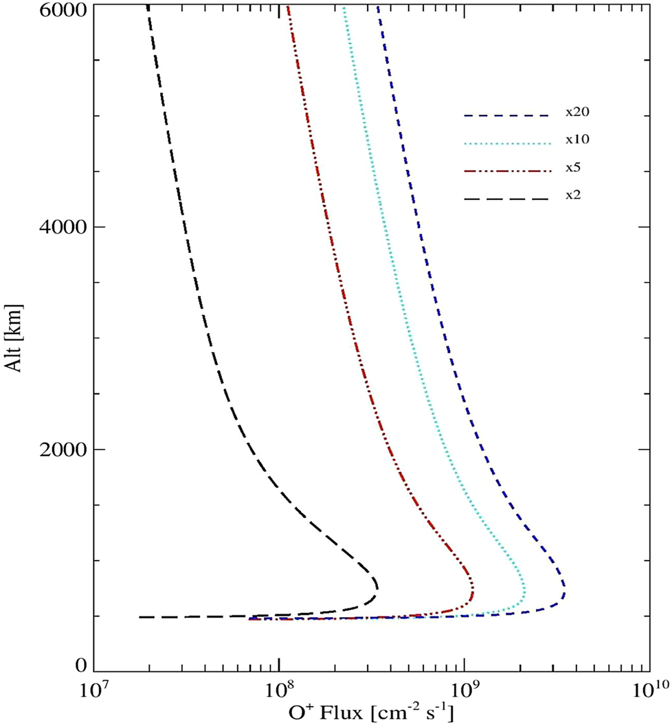
Fig. 14. The mass loss rate of oxygen ions from the Earth atmosphere due to XUV flux from the young Sun at F XUV = 2F 0 (long dash), 5F 0 (dash-dot), 10F 0 (dot) and 20F 0 (short dash) (from Airapetian et al., Reference Airapetian, Glocer, Khazanov, Loyd, ROP, France, K, Sojka, J, Danchi, WC and Liemohn, MW2017a).
This relation represents the low bound for the ion escape rate, because it does not consider the ionospheric heating due to precipitating electrons during storms. Such additional heating swells the ionosphere, and thus enhances the escape rate. XUV and electron precipitation driven ion escape fluxes should be quite large for many close-in exoplanets around M dwarfs or young K stars as their XUV fluxes are 100–400F 0 and can retain such high-XUV emission fluxes over 1 Gyr. This will make it difficult for such planets to retain their atmospheres over the geological timescales unless considerable atmospheres are outgassed from the interior via volcanic outgassing during later phases of planetary evolution. In order to develop the complete picture of atmospheric escape from close-in exoplanets, these effects should be studied with future multi-dimensional hydrodynamic and kinetic models with inclusion of XUV and electron precipitation induced heating.
Impact of space weather on atmospheric chemistry of early Earth and Mars
Dynamics of early atmospheres of Earth, Venus and Mars
The very first atmospheres (‘proto-atmospheres’) of Earth, Venus and Mars (excluding the initial silicate-containing envelope formed during accretion) consisted of a thick envelope of molecular hydrogen (H2) with up to several hundreds of bars of surface pressure accreted directly from the protoplanetary disc. These proto-atmospheres were likely lost within a few million years after planetary formation due to rapid escape driven by strong EUV emissions by the active early Sun (e.g. Lammer et al., Reference Lammer, Zerkle, Gebauer, Tosi, Noack, Scherf, Pilat-Lohinger, Güdel, Grenfell, Godolt and Nikolaou2018). They were followed by a thick (with up to hundreds of bar surface pressure) steam atmosphere phase which arose due to volatile degassing and which lasted approximately from the magma ocean phase up to tens to hundreds of Myr after formation of the crust (see e.g. Zahnle et al., 1988; Elkins-Tanton, Reference Elkins-Tanton2012; Lammer et al., Reference Lammer, Zerkle, Gebauer, Tosi, Noack, Scherf, Pilat-Lohinger, Güdel, Grenfell, Godolt and Nikolaou2018; Nikolaou et al., Reference Nikolaou, Katyal, Tosi, Godolt, Grenfell and Rauer2019). This process is followed by formation of a secondary atmosphere of heavier gases, such as N2–CO2 rich environment as the planet cools and its surface solidifies (Elkins-Tanton, Reference Elkins-Tanton2008; Noack et al., Reference Noack, Godolt, von Paris, Plesa, Stracke, Breuer and Rauer2014).
Comparative studies of the effect of the active young Sun on the atmospheric evolution of Earth, Venus and Mars were performed by Kulikov et al. (Reference Kulikov, Lammer, Lichtenegger, Terada, Ribas, Kolb, Langmayr, Lundin, Guinan, Barabash and Biernat2006), Johnstone et al. (Reference Johnstone, Güdel, Lammer and Kislyakova2018, Reference Johnstone, Khodachenko, Lüftinger, Kislyakova, Lammer and Güdel2019), Baines et al. (Reference Baines, Atreya, Bullock, Grinspoon, Mahaffy, Russell, Schubert, Zahnle and Mackwell2013), Lammer et al. (Reference Lammer, Zerkle, Gebauer, Tosi, Noack, Scherf, Pilat-Lohinger, Güdel, Grenfell, Godolt and Nikolaou2018), Tian et al. (Reference Tian, Güdel, Johnstone, Lammer, Luger and Odert2018) and Airapetian et al. (Reference Airapetian, Glocer, Gronoff, Hébrard and Danchi2016, Reference Airapetian, Danchi, Dong, Rugheimer, Mlynczak, Stevenson, Henning, Grenfell, Jin, Glocer, Gronoff, Lynch, Johnstone, Lueftinger, Guedel, Kobayashi, Fahrenbach, Hallinan, Stamenkovic, Cohen, Kuang, van der Holst, Manchester, Zank, Verkhoglyadova, Sojka, Maehara, Notsu, Yamashiki, France, Lopez Puertas, Funke, Jackman, Kay, Leisawitz and Alexander2018a, Reference Airapetian, Adibekyan, Ansdell, Cohen, Cuntz, Danchi, Dong, Drake, Fahrenbach, France, Garcia-Sage, Glocer, Grenfell, Gronoff, Hartnett, Henning, Hinkel, Jensen, Jin, Kalas, Kane, Kobayashi, Kopparapu, Leake, López-Puertas, Lueftinger, Lynch, Lyra, Mandell, Mandt, Moore, Nna-Mvondo, Notsu, Maehara, Yamashiki, Shibata, Oman, Osten, Pavlov, Ramirez, Rugheimer, Schlieder, Schnittman, Shock, Sousa-Silva, Way, Yang, Young and Zank2018b), who emphasized that comparative atmospheric evolution could only be understood in the context of an evolving Sun. Specifically, flare-driven XUV emission and the dense fast wind and associated frequent and associated CMEs from the young Sun could have been an important factor in setting habitability conditions on early terrestrial planets (Airapetian, Reference Airapetian2018b). Its consequences on the magnetosphere and thermosphere of early Earth and Mars are the area of emerging research (Airapetian et al., Reference Airapetian, Glocer, Gronoff, Hébrard and Danchi2016, Reference Airapetian, Danchi, Dong, Rugheimer, Mlynczak, Stevenson, Henning, Grenfell, Jin, Glocer, Gronoff, Lynch, Johnstone, Lueftinger, Guedel, Kobayashi, Fahrenbach, Hallinan, Stamenkovic, Cohen, Kuang, van der Holst, Manchester, Zank, Verkhoglyadova, Sojka, Maehara, Notsu, Yamashiki, France, Lopez Puertas, Funke, Jackman, Kay, Leisawitz and Alexander2018a, Reference Airapetian, Adibekyan, Ansdell, Cohen, Cuntz, Danchi, Dong, Drake, Fahrenbach, France, Garcia-Sage, Glocer, Grenfell, Gronoff, Hartnett, Henning, Hinkel, Jensen, Jin, Kalas, Kane, Kobayashi, Kopparapu, Leake, López-Puertas, Lueftinger, Lynch, Lyra, Mandell, Mandt, Moore, Nna-Mvondo, Notsu, Maehara, Yamashiki, Shibata, Oman, Osten, Pavlov, Ramirez, Rugheimer, Schlieder, Schnittman, Shock, Sousa-Silva, Way, Yang, Young and Zank2018b; Dong et al., Reference Dong, Lingam, Ma and Cohen2017). As discussed in the section ‘Winds from active stars’, the frequency of a Carrington-scale flare event from the young Sun at 0.7 Gyr was about one event per day that suggests that such events could have been accompanied by a super-CME of a comparable energy (Airapetian et al., Reference Airapetian, Glocer, Gronoff, Hébrard and Danchi2016; Alvarado-Gómez et al., Reference Alvarado-Gómez, Drake, Cohen, Moschou and Garraffo2018). Recent study suggests that the reflection of CMEs from coronal holes of the young Sun deviated from radial path towards the equator, and thus increased the resulting frequency of ‘geoeffective’ CMEs (with the southward directed z-component of the magnetic field, which is opposite to the Earth's magnetospheric field) that may hit the Earth and cause strong GM (Kay et al., Reference Kay, Gopalswamy, Reinard and Opher2017).
As an energetic geoeffective Carrington-type CME propagating in the background of the solar wind from the young Sun (or an active star) moves towards the early Earth (or a young Earth-like planet), its dynamic pressure compresses and convects the planetary magnetospheric field inducing the convective electric field and associated ionospheric current. Thus, the shape of the Earth's magnetosphere is the result of the interaction with the dense and fast wind from the young Sun (Airapetian and Usmanov, Reference Airapetian and Usmanov2016). The distance of subsolar magnetosphere from the Earth's surface varies in times in response to the changing dynamic pressure from the solar wind and a CME. Its boundary known as the standoff distance is determined from the balance between the magnetic pressure of the Earth magnetosphere and the wind dynamic pressure. The larger the dynamic pressure, $\rho V_{\rm w}^2$ , the smaller is the standoff distance. The solar wind and a CME also compress the night-side magnetosphere and ignite magnetic reconnection at the night-side of the Earth's magnetosphere causing the magnetospheric storm as particles penetrate the polar regions of Earth. Also, the orientation of the magnetic field of the wind and CME as compared to that of the Earth's magnetospheric field controls the energy transfer from the wind to the planet, as it drives magnetic reconnection which in turn ignites particle acceleration and particle precipitation in the planetary ionosphere and thermosphere (e.g. Kivelson and Russell, Reference Kivelson, Russell, Kivelson and Russell1995; Tsurutani et al., Reference Tsurutani, Mannucci, Iijima, Guarnieri, Gonzalez, Judge, Gangopadhyay and Pap2006). This process is driven by electric fields that accelerate the ions against the neutrals resulting in current dissipation (Ohmic or Joule heating). In addition, the particle precipitation in the upper atmosphere impacts the local ionization and modifies Joule heating processes (see e.g. Deng et al., Reference Deng, Fuller-Rowell, Akmaev and Ridley2011 and references therein) and atmospheric line excitation (i.e. auroral excitation, Schunk and Nagy, Reference Schunk and Nagy1980).
The simulations of the interaction of a Carrington-type CME with the early Earth's magnetosphere are shown in Fig. 15. The left panel of Fig. 15 shows that the magnetospheric standoff distance moves from ~10R E (right panel) to ~1.5R E as the Carrington scale CME from the young Sun with the southwards Bz component of the magnetic field as a result of the combined effect of magnetic reconnection between two fields and the CME dynamic pressure (Airapetian et al., Reference Airapetian, Glocer, Danchi and Gronoff2015, Reference Airapetian, Glocer, Gronoff, Hébrard and Danchi2016; right panel of Fig. 15). The boundary of the magnetospheric open-closed field shifts to 36° in latitude opening 70% of the Earth's magnetic field. The CME dynamic pressure drives large field aligned electric currents that dissipates in the ionosphere–thermosphere region (at ~110 km) of the Earth via ion-neutral frictional resistivity producing Joule heating rate reaching ~4 W m−2. This is over 20 times larger than that observed during largest GM, and will thus increase the upper atmospheric temperature and ignite enhanced ionospheric outflow (Airapetian et al., Reference Airapetian, Glocer, Khazanov, Loyd, ROP, France, K, Sojka, J, Danchi, WC and Liemohn, MW2017a). The models of associated atmospheric escape are in their infancy and require the extension of sophisticated tools to consider multi-fluid effects for consistent treatment of neutral species in the ionosphere–thermosphere dynamics developed for the current and early Earth, Mars and Titan (Smithtro and Sojka, Reference Smithtro and Sojka2005; Ridley et al., Reference Ridley, Deng and Tóth2006; Bell, Reference Bell2008; Tian et al., Reference Tian, Solomon, Qian, Lei and Roble2008; Glocer et al., Reference Glocer, Kitamura, Toth and Gombosi2012; Johnstone et al., Reference Johnstone, Güdel, Lammer and Kislyakova2018).
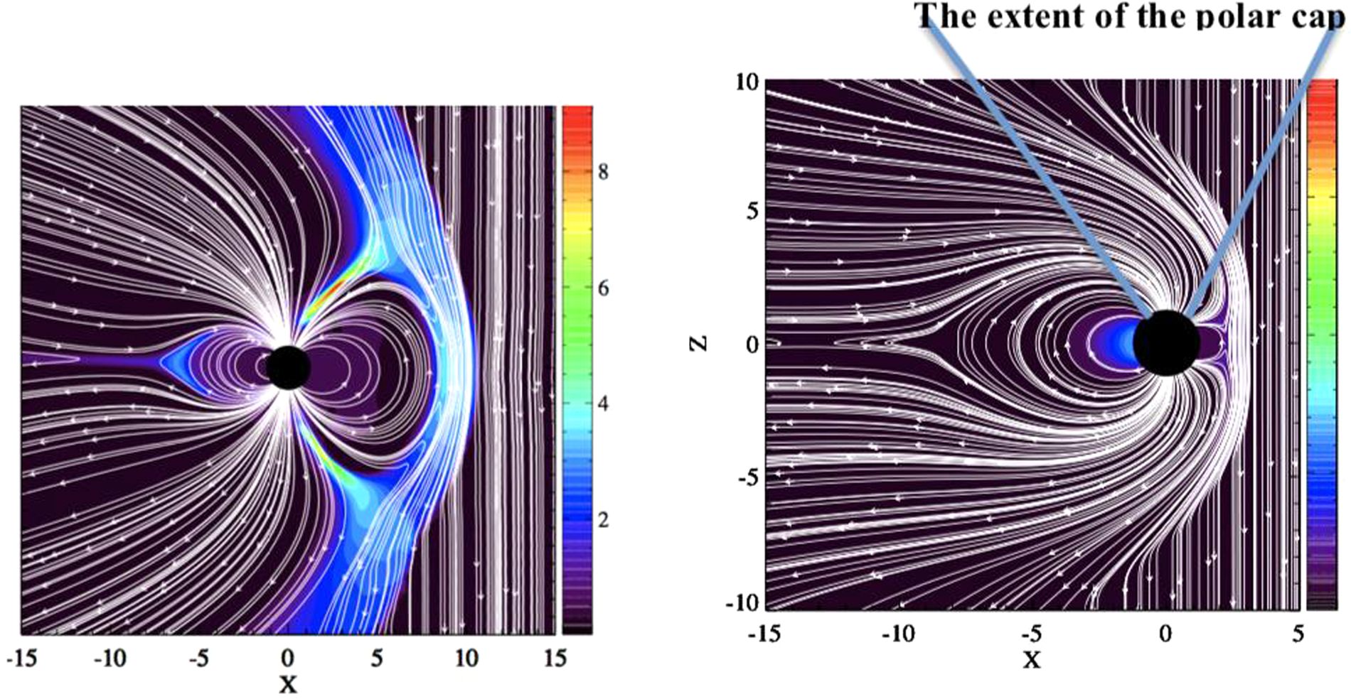
Fig. 15. The magnetic-field lines and plasma pressure in the Earth's magnetosphere due to a CME event: (a) initial state and (b) final state. Magnetic-field lines (white) and plasma pressure in nPa (colour map). Axes represent distance from the Earth's centre in units of Earth radius (Airapetian et al., Reference Airapetian, Glocer, Gronoff, Hébrard and Danchi2016).
Early Earth. Lammer et al. (Reference Lammer, Zerkle, Gebauer, Tosi, Noack, Scherf, Pilat-Lohinger, Güdel, Grenfell, Godolt and Nikolaou2018) suggested that proto-Earth was formed via planetesimal accretion growing to 0.5–0.75M Earth in about 10 Myr. The accretion phase is characterized by the formation of magma oceans surrounded with a nebular-captured H2-rich envelope (primary atmosphere) and delivery of volatiles via impactors formed in the outer Solar System. High XUV driven by the young Sun heating via photoionization ignited hydrodynamic escape of the atmosphere (Erkaev et al., Reference Erkaev, Lammer, Elkins-Tanton, Stökl, Odert, Marcq, Dorfi, Kislyakova, Kulikov, Leitzinger and Güdel2014; Owen and Mohanty, Reference Owen and Mohanty2016). As the steam atmosphere later collapses or erodes via escape processes, magma ocean will finally solidify, and thus promote the formation of Earth's oceans. Continued outgassing produced the secondary atmosphere could have been dominated by H2O and CO2 with a minor amount of N2 and traces of inert gases, hydrocarbons (e.g. CH4), and sulphur-containing compounds or by more reduced atmosphere depending on the redox state of mantle (see e.g. Schaefer and Fegley, Reference Schaefer and Fegley2017; Lammer et al., Reference Lammer, Zerkle, Gebauer, Tosi, Noack, Scherf, Pilat-Lohinger, Güdel, Grenfell, Godolt and Nikolaou2018). Numerous geochemical proxies exist which constrain the Archaean atmosphere. For example, Rosing et al. (Reference Rosing, Bird, Sleep and Bjerrum2010) suggested that magnetite siderite equilibria in banded iron minerals implied that atmospheric CO2 concentrations did not exceed (~×3) the present atmospheric level on the early Earth, although this view is contested (Kasting, Reference Kasting2010). The evolution of N2 is even more uncertain (Wordsworth, Reference Wordsworth2016; Lammer et al., Reference Lammer, Zerkle, Gebauer, Tosi, Noack, Scherf, Pilat-Lohinger, Güdel, Grenfell, Godolt and Nikolaou2018). Recent study of evolution of molecular nitrogen by Gebauer et al. suggests atmospheric pressure of early Archaean Earth was less than 0.5 bar slowly rising in time due to diminishing effects of N2 reduction via atmospheric escape and nitrogen fixation. Som et al. (Reference Som, Catling, Harnmeijer, Polivka and Buick2012) suggested that atmospheric pressure was less than ~2 bar during the late Archaean based upon an analysis of the size distribution of fossilized raindrop imprints. They revised this estimate to less than half of present levels in recent work (Som et al., Reference Som, Buick, Hagadorn, Blake, Perreault, Harnmeijer and Catling2016). Marty et al. (Reference Marty, Zimmermann, Pujol, Burgess and Philippot2013) argue that Archaean N2 levels were 0.5–1.1 bar, with 0.7 bar or less of CO2. This is consistent with the evolutionary scenarios of N2 atmospheric pressure at 2.7 Gyr. Such low atmospheric pressure makes it difficult to explain the warming of the Archaean Earth via recently proposed scenarios (Goldblatt et al., Reference Goldblatt, Claire, Lenton, Matthews, Watson and Zahnle2009). To warm the atmosphere, a strong greenhouse gas is required. Airapetian et al. (Reference Airapetian, Glocer, Gronoff, Hébrard and Danchi2016) have recently suggested that a potent greenhouse gas, nitrous oxide (N2O) can be efficiently formed via frequent energetic particle precipitation into the lower Archaean atmosphere driven by SEP events from the young Sun.
Oxygen isotope data in cherts could constrain paleo ocean temperatures (see e.g. discussion in Shields and Kasting (Reference Shields and Kasting2007)). Molybdenum (Anbar et al., Reference Anbar, Duan, Lyons, Arnold, Kendall, Creaser, Kaufman, Gordon, Scott, Garvin and Buick2007) data suggest early ‘whiffs’ of atmospheric oxygen as a prelude to the Great Oxidation Rise which marked the end of the Archaean (Lyons et al., Reference Lyons, Reinhard and Planavsky2014; Smit and Mezger, Reference Smit and Mezger2017). Loss of mass independent fractionation of sulphur isotopes observed near the end of the Archaean could imply either a rise in atmospheric oxygen and/or a decrease in atmospheric methane (Zahnle et al., Reference Zanhle, Claire and Catling2006). Finally, flow features preserved in ancient soil (paleosols) suggest the presence of liquid water despite the fainter early Sun – this issue is described in more detail in the habitability discussion in section 6.3.
In summary, the Earth's atmosphere has undergone extremely strong and (in geological terms) rapid change both in composition and mass during its evolutionary history. More work is however required to constrain the detailed effects of SW, especially the interaction of energetic XUV emission and high-energy particles during the various phases of atmospheric evolution of our planet.
Early Venus. Measurements of the deuterium to hydrogen (D/H) ratio taken from the clouds of Venus by the Pioneer Venus Mission (Donahue et al., Reference Donahue, Hoffman, Hodges and Watson1982) suggest at least 150-fold enhancement compared with terrestrial water. This high fractionation of deuterium suggests that the planet underwent considerable water loss during its evolution and that conditions on early Venus could have been habitable. Way et al. (Reference Way, Del Genio, Kiang, Sohl, Grinspoon, Aleinov and Clune2016) summarize possible scenarios of the water evolution on early Venus. They note that the early water inventory was likely lost within ~100 Myr after formation due to atmospheric escape driven by XUV flux from the active young Sun (see also Chassefiere, Reference Chassefiere1997; Ramirez and Kaltenegger, Reference Ramirez and Kaltenegger2014). Since paleo estimates suggest the equivalent of 19 to 500 m water covering the surface, this requires considerable water delivery during the late veneer (Donahue and Russell, Reference Donahue, Russell, Baugher, Hunten and Phillips1997). Wordsworth (Reference Wordsworth2016) discusses possible mechanisms for the presently observed elevated amount of N2 in Venus’ atmosphere relative to that of Earth.
Early Mars. A wealth of geological proxies (e.g. geophysical flow features, clay deposition, etc.) suggests that early Mars could have experienced habitable periods during its evolutionary history (Ramirez and Craddock, Reference Ramirez and Craddock2018). Tian et al. (Reference Tian, Kasting and Solomon2009) had applied an upper atmospheric model to study the evolution of the Martian atmosphere and found that a dense primordial CO2 atmosphere could not have been maintained. Later work by Erkaev et al. (Reference Erkaev, Lammer, Elkins-Tanton, Stökl, Odert, Marcq, Dorfi, Kislyakova, Kulikov, Leitzinger and Güdel2014) confirmed that of Tian et al. (Reference Tian, Kasting and Solomon2009) suggesting that several tens of bar of CO2 (via catastrophic outgassing after the magma ocean solidified) could be quickly lost (within about 12 million years) due to extreme stellar-XUV-driven escape arising from the active young sun. Outgassing and (possibly) delivery led to the subsequent build-up of up to ~1 bar atmospheric pressure (Kite et al., Reference Kite, Williams, Lucas and Aharonson2014) on early Mars which could have favoured habitable conditions. Analogous to the early Earth, earlier numerical models mostly predicted surface temperatures below freezing on early Mars despite geoproxy data to the contrary (e.g. Craddock and Howard, Reference Craddock and Howard2002). To address this issue, the model study by Ramirez et al. (Reference Ramirez, Kopparapu, Zugger, Robinson, Freedman and Kasting2014) suggested that the presence of 1.3–4 bar of CO2, 5–20% H2 could enhance the efficiency of the early Martian greenhouse in order to attain habitable surface conditions. Von Paris et al. (Reference von Paris, Grenfell, Rauer and Stock2013) suggested up to 13 K surface warming on adding 0.5 bar N2(g). Wordsworth et al. (Reference Wordsworth, Kalugina, Lokshtanov, Vigasin, Ehlmann, Head and Wang2017) suggested that updating previously underestimated collision-induced absorption could lead to significant warming. Ramirez (Reference Ramirez2017) subsequently found that H2 concentrations as low as 1% can sustain mean surface temperatures above freezing. Related model studies of early Mars-type environments investigated factors impacting habitability, e.g. clouds (Urata and Toon, Reference Urata and Toon2013; Kitzmann, Reference Kitzmann2017; Ramirez and Kasting, Reference Ramirez and Kasting2017), the effects of surface ice (Ramirez, Reference Ramirez2017) and precipitation (von Paris et al., Reference von Paris, Petau, Grenfell, Hauber, Breuer, Jaumann, Rauer and Tirsch2015). Detailed 3D model studies of the early Martian climate have been performed (Forget et al., Reference Forget, Wordsworth, Millour, Madeleine, Kerber, Leconte, Marcq and Haberle2013; Wordsworth et al., Reference Wordsworth, Kerber, Pierrehumbert, Forget and Head2015) which investigate the response of surface habitability to varying e.g. atmospheric composition, mass and planetary orbital parameters.
Detailed studies of the effects of SW upon the evolution of early Mars – in terms of e.g. enhanced EUV absorption and particle induced ionization during air-shower events – are to our knowledge rather lacking in the literature. In particular, studies which focus on the Noachian and Hesperian periods including SW effects and assuming representative atmospheres i.e. CO2 (~1–5 bar); N2 (<0.5 bar); H2 (<a few tenths of a bar) and CH4 (<a few hundredths of a bar) (as quoted in the literature and discussed above) would be desirable.
Impacts of space weather on close-in exoplanets
Effect on habitability of Proxima b
Proxima Centauri constitutes the third and smallest member of the triple star system Alpha Centauri which, with only 1.3 pc (4.4 light-years) distance from Earth, are the closest stars to our Solar System. The only known planet in this star system is Proxima Centauri b (Anglada-Escudé et al., Reference Anglada-Escudé, Amado, Barnes, Berdiñas, Butler, Coleman, de La Cueva, Dreizler, Endl, Giesers, Jeffers, Jenkins, Jones, Kiraga, Kürster, López-González, Marvin, Morales, Morin, Nelson, Ortiz, Ofir, Paardekooper, Reiners, Rodríguez, Rodríguez-López, Sarmiento, Strachan, Tsapras, Tuomi and Zechmeister2016), hereafter Proxima b, with a minimum mass of 1.27M and an orbital period of 11.2 days i.e. clearly located in the CHZ (following Kopparapu et al., Reference Kopparapu, Ramirez, Kasting, Eymet, Robinson, Mahadevan, Terrien, Domagal-Goldman, Meadows and Deshpande2013). The planet is only inferred from radial velocity measurements and the probability of Proxima b of transiting is very small (Kipping et al., Reference Kipping, Cameron, Hartman, Davenport, Matthews, Sasselov, Rowe, Siverd, Chen and Sandford2017). Little is known about Proxima b's upper mass limit, although it could be rocky based on planetary population statistics from the Kepler mission (Weiss and Marcy, Reference Weiss and Marcy2014). It is also still unclear from the data whether there could be more planets around this M5.5V red dwarf star with its effective temperature T eff of 3050 K (Anglada-Escudé et al., Reference Anglada-Escudé, Amado, Barnes, Berdiñas, Butler, Coleman, de La Cueva, Dreizler, Endl, Giesers, Jeffers, Jenkins, Jones, Kiraga, Kürster, López-González, Marvin, Morales, Morin, Nelson, Ortiz, Ofir, Paardekooper, Reiners, Rodríguez, Rodríguez-López, Sarmiento, Strachan, Tsapras, Tuomi and Zechmeister2016; Barnes et al., Reference Barnes, Deitrick, Luger, Driscoll, Quinn, Fleming, Guyer, McDonald, Meadows and Arney2016). Proxima Cen is a highly active star with flaring events of ~1030 erg once a day and low energy events (~1028 erg) every hour (Walker, Reference Walker1981; Davenport, Reference Davenport2016). This compares to the largest recorded solar SEP events e.g. SEP 1989 and the Carrington event (Atri, Reference Atri2017). Proxima Cen's surface magnetic field (B ~ 600 G) is orders of magnitudes larger than on our Sun (Reiners and Basri, Reference Reiners and Basri2008). Additionally, the total stellar irradiation (TSI) was found to vary significantly by about 17% over Proxima Cen's rotation period of 83 days, which might have a crucial impact on the atmospheric evolution of Proxima b which receives an average TSI of 65% of the Earth (Anglada-Escudé et al., Reference Anglada-Escudé, Amado, Barnes, Berdiñas, Butler, Coleman, de La Cueva, Dreizler, Endl, Giesers, Jeffers, Jenkins, Jones, Kiraga, Kürster, López-González, Marvin, Morales, Morin, Nelson, Ortiz, Ofir, Paardekooper, Reiners, Rodríguez, Rodríguez-López, Sarmiento, Strachan, Tsapras, Tuomi and Zechmeister2016).
There are numerous factors e.g. planetary mass, orbital evolution and atmospheric properties, which influence habitability (Kasting et al., Reference Kasting, Whitmire and Reynolds1993; Wordsworth et al., Reference Wordsworth, Forget and Eymet2010; Pierrehumbert, Reference Pierrehumbert2011; Kopparapu et al., Reference Kopparapu, Ramirez, Kasting, Eymet, Robinson, Mahadevan, Terrien, Domagal-Goldman, Meadows and Deshpande2013). Since Proxima b is non-transiting, the key parameter ranges determining the state of Proxima b's atmosphere are large. Proxima b could have formed either at its current semi-major axis or maybe beyond the snow line, and for both cases there are parameter ranges for which it could still possess a significant amount of water (Carter-Bond et al., Reference Carter-Bond, O'Brien and Raymond2012; Ciesla et al., Reference Ciesla, Mulders, Pascucci and Apai2015; Mulders et al., Reference Mulders, Ciesla, Min and Pascucci2015). Given that the presence of water is, by definition, essential for the study of habitability, numerous model studies have shown scenarios for which Proxima b could support periods of liquid water, depending on e.g. the H2, O2 and CO2 evolution of its atmosphere (Luger et al., Reference Luger, Barnes, Lopez, Fortney, Jackson and Meadows2015; Barnes et al., Reference Barnes, Deitrick, Luger, Driscoll, Quinn, Fleming, Guyer, McDonald, Meadows and Arney2016; Meadows et al., Reference Meadows, Arney, Schwieterman, Lustig-Yaeger, Lincowski, Robinson, Domagal-Goldman, Deitrick, Barnes, Fleming, Luger, Driscoll, Quinn and Crisp2018a; Ribas et al., Reference Ribas, Bolmont, Selsis, Reiners, Leconte, Raymond, Engle, Guinan, Morin, Turbet, Forget and Anglada-Escudé2016). While assuming the best-case scenario of a rocky, low-mass planet, Turbet et al. (Reference Turbet, Leconte, Selsis, Bolmont, Forget, Ribas, Raymond and Anglada-Escudé2016) and Boutle et al. (Reference Boutle, Mayne, Drummond, Manners, Goyal, Lambert, Acreman and Earnshaw2017) have shown in 3D Global Climate Model (GCM) studies that water is more likely to be present if Proxima b is tidally-locked, at least at the sub-stellar point. Del Genio et al. (Reference Del Genio, Way and Amundsen2017) found the possibility of an even broader region of liquid water with their 3D-GCM studies including a dynamic ocean.
Can the environments of such close-in terrestrial-type planets within CHZ from their parent stars be hospitable to life? This answer requires the conditions of SW around red dwarf stars including quiescent and flare-driven XUV fluxes and their properties of stellar winds.
The XUV emission from Proxima Centauri was recently presented by Garcia-Sage et al. (Reference Garcia-Sage, Glocer, Drake, Gronoff and Cohen2017). They used the reconstructed XUV fluxes that appear to be over 2 orders of magnitude greater at the planet location than that received by the Earth to evaluate the associated ion escape. The calculated escaping O+ mass flux from Proxima Cen b appears to be high as presented in Fig. 19, consistent with the results of Airapetian et al. (Reference Airapetian, Glocer, Khazanov, Loyd, ROP, France, K, Sojka, J, Danchi, WC and Liemohn, MW2017a). They also discussed the impact of thermospheric temperature and polar cap area on the escape fluxes. A hotter thermosphere is obviously expected to result in stronger outflows, but a larger polar cap area (the area of open magnetic flux connected to the stellar wind) also results in more net mass flux of ionized particles lost to space. Figure 16 shows the connection between these quantities and the mass loss rate. As expected, the thermospheric temperature and the polar cap size have strong implications for the mass loss rate at Proxima Cen b and the ability for this exoplanet to retain its atmosphere on geological timescale.
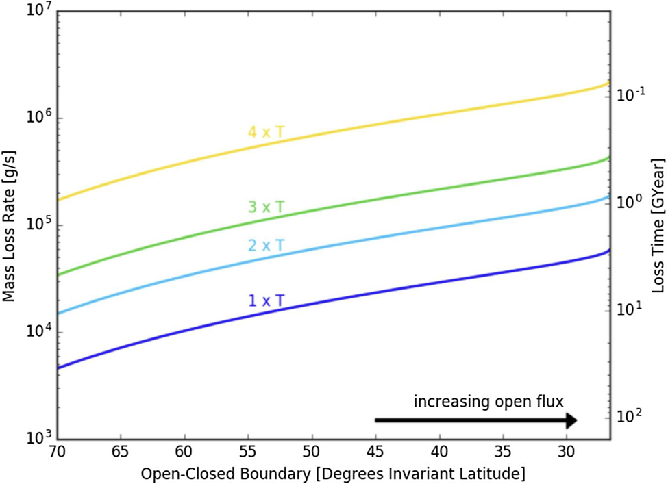
Fig. 16. The ion escape rate calculated for four different neutral thermospheric temperatures of Proxima b driven by XUV fluxes from Proxima Cen (Garcia-Sage et al., Reference Garcia-Sage, Glocer, Drake, Gronoff and Cohen2017).
In summary, due to its proximity to the star, Proxima Cen b resides in an extremely hostile and extreme space environment that is likely to cause high atmospheric loss rates. If it is not clear whether the planet can sustain an atmosphere at all, it is less likely that the planet is habitable, even though it resides in the CHZ around the star.
The effects of stellar wind from Proxima Centauri on its exoplanet have recently been characterized by Garraffo et al. (Reference Garraffo, Drake and Cohen2016). They have theoretically reconstructed the stellar wind from Proxima Centauri and modelled the space environment conditions around Proxima Cen b. The model of the stellar coronal wind was driven by magnetic-field observations (ZDI map) of the star GJ 51, which was used as a proxy for Proxima Cen for which ZDI observations are not available. Following the limited information about the magnetic field of Proxima Cen (Reiners and Basri, Reference Reiners and Basri2008), they used two cases of average stellar magnetic field of 300 and 600 G. They found that the stellar wind's dynamic and magnetic pressure along the orbit of Proxima Cen b are extremely large, up to 20 000 times that of the solar wind at 1 AU. In addition, the planet experiences fast and very large variations in the ambient pressure along its orbit. As a result, the magnetosphere surrounding the planet undergoes huge variations within the relatively short period of the orbit, which potentially drive strong currents in the upper atmosphere and result in extreme atmospheric heating (see Fig. 17). The combination of extreme XUV fluxes and the ambient wind pressure, along with the fast and strong variations, potentially make the atmosphere of Proxima Cen b highly vulnerable to strong atmospheric stripping by the stellar wind, and atmospheric escape as a result of the additional strong heating. The simulations suggest that Proxima Cen b may reside in the sub-Alfvenic stellar wind at least part of the orbit, which removes the magnetopause completely, and exposes the planetary atmosphere to direct impact by stellar wind particles.
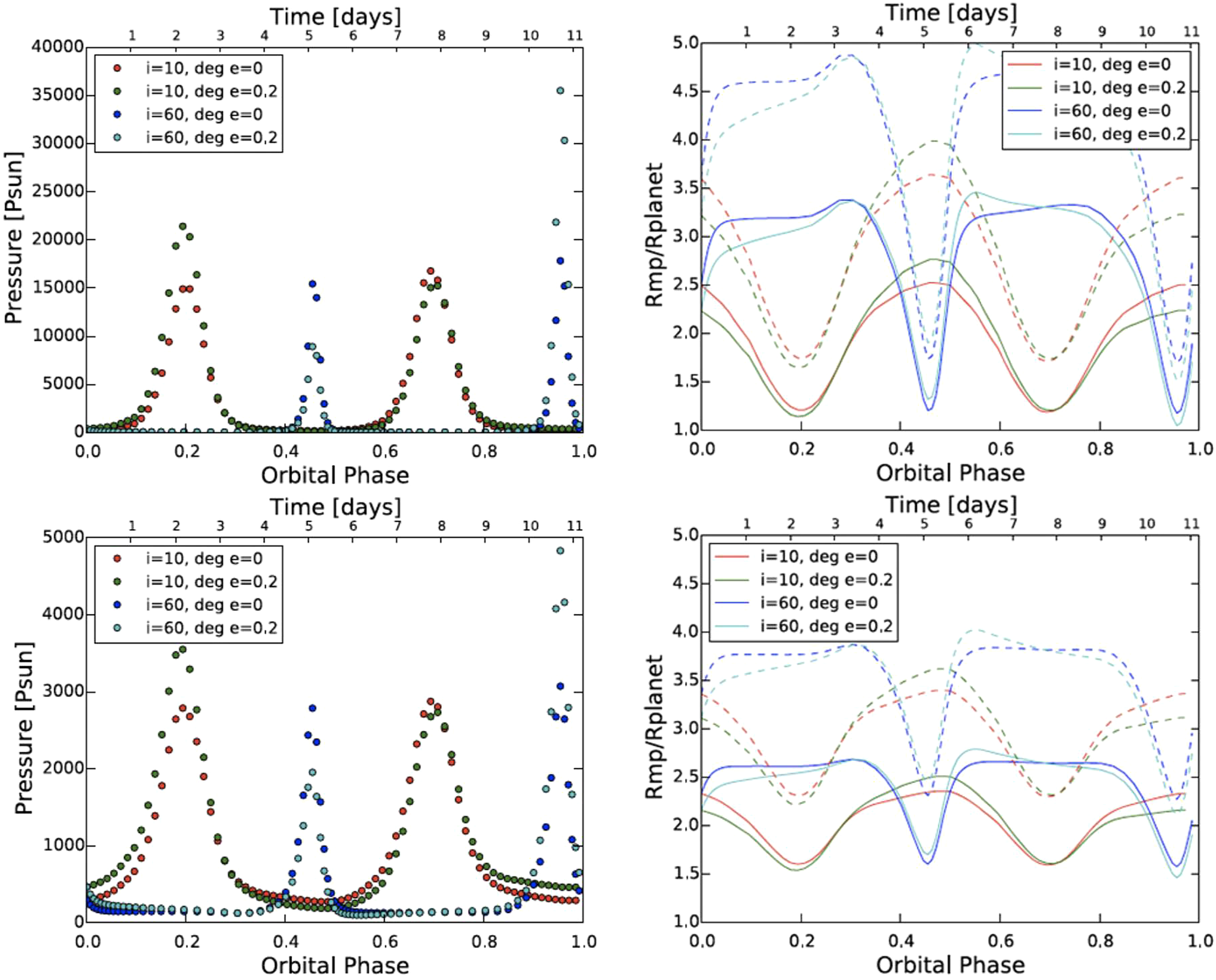
Fig. 17. Left: Dynamic pressure along the possible orbits of Proxima Cen b normalized to typical dynamic pressure of the solar wind at 1 AU for stellar field maximum of 600 G (top) and mean of 600 G (bottom). Right: Same but plots show the magnetosphere standoff distance (from Garraffo et al., Reference Garraffo, Drake and Cohen2016).
Effect on habitability of the TRAPPIST-1 system
The recently discovered TRAPPIST-1 planetary system (Gillon et al., Reference Gillon, Jehin, Lederer, Delrez, de Wit, Burdanov, Van Grootel, Burgasser, Triaud, Opitom, Demory, Sahu, Gagliuffi, Magain and Queloz2016) is 39 light-years away and contains a so-called ultra-cool magnetically active M8.2V dwarf star, surrounded by seven terrestrial-type exoplanets three of which, d, e and f, could be located within the CHZ and have orbital periods of 4, 6 and 9 days, respectively (Kopparapu et al., Reference Kopparapu, Wolf, Arney, Batalha, Haqq-Misra, Grimm and Heng2017). TRAPPIST-1 has a low T eff of around 2560 K and (similar to Proxima Cen) exhibits strong surface (~600 G) magnetic fields driving intensive chromospheric activity (Reiners and Basri, Reference Reiners and Basri2008) accompanied by frequent (0.38 per day) stellar flares with energies between 1030 and 1033 erg (Vida et al., Reference Vida, Kővári, Pál, Oláh and Kriskovics2017). Unlike Proxima Cen, TRAPPIST-1 is a known transiting planetary system, which constrains the possible planetary parameters significantly. TRAPPIST-1b and c receive a greater stellar flux than Venus and are therefore suggested to have undergone a runaway greenhouse, or might still be in the runaway phase (Bourrier et al., Reference Bourrier, de Wit, Bolmont, Stamenković, Wheatley, Burgasser, Delrez, Demory, Ehrenreich, Gillon, Jehin, Leconte, Lederer, Lewis, Triaud and Van Grootel2017). Recent numerical studies by Wordsworth et al. (Reference Wordsworth, Kalugina, Lokshtanov, Vigasin, Ehlmann, Head and Wang2017) have shown that abiotic O2 build-up is possible for lose-in planets within the CHZ, which makes them interesting targets for biosignature studies. On the other hand, the lower stellar flux on TRAPPIST-1f and g makes abiotic O2 build-up unlikely, hence they are excellent targets for atmospheric characterization follow-ups.
Model studies by Barstow and Irwin (Reference Barstow and Irwin2016) estimated that Earth's present-day ozone levels should be detectable with JWST on planets b, c, and d with observations of 30–60 transits. Recent hydrodynamic escape studies suggest that planets accreted wet (many Earth oceans of water), although this is generally debated at this point (Tian and Ida, Reference Tian and Ida2015). Bolmont et al. (Reference Bolmont, Selsis, Owen, Ribas, Raymond, Leconte and Gillon2017) and Bourrier et al. (Reference Bourrier, de Wit, Bolmont, Stamenković, Wheatley, Burgasser, Delrez, Demory, Ehrenreich, Gillon, Jehin, Leconte, Lederer, Lewis, Triaud and Van Grootel2017) estimate that the inner planets likely lost most of their water, whereas planets d, e, f, g and h could have retained all but a few Earth oceans, depending on the age of the system. Furthermore, 3D global climate models of the TRAPPIST-1 system, which are able to consider tidal-locking, have controversially shown that the accumulation of greenhouse gases could be difficult for all planets in the system (Yang et al., Reference Yang, Cowan and Abbot2013). This is because CO2 likely freezes out on the night side, and the high EUV flux rapidly photodissociates NH3 and CH4. In the case that CO2 can eventually build up, planets e, f and g could sustain liquid water (Turbet et al., Reference Turbet, Bolmont, Leconte, Forget, Selsis, Tobie, Caldas, Naar and Gillon2017, Reference Turbet, Bolmont, Leconte, Forget, Selsis, Tobie, Caldas, Naar and Gillon2018). However, we should be cautious with aforementioned results that do not account for the O+ escape rates due to XUV fluxes and orbital environments as discussed in the previous subsection (Garraffo et al., Reference Garraffo, Drake and Cohen2016; Airapetian et al., Reference Airapetian, Glocer, Khazanov, Loyd, ROP, France, K, Sojka, J, Danchi, WC and Liemohn, MW2017a; Garcia-Sage et al., Reference Garcia-Sage, Glocer, Drake, Gronoff and Cohen2017). These factors may prevent the build-up of O2 and subsequent formation of ozone in atmospheres of these planets and need to be modelled with the impacts of SW effects from their host star. Another important impact on atmospheric escape may come from interaction of stellar winds with exoplanets. Specifically, strongly magnetized wind from TRAPPIST-1 introduces a strong dynamic pressure up to a factor of 1000 solar-wind pressure on Earth on hypothetical exoplanetary magnetospheres. As exoplanets orbit the star, the wind pressure changes by an order of magnitude and most planets spend a large fraction of their orbital period in the sub-Alfvenic regime (Garraffo et al., Reference Garraffo, Drake and Cohen2016). Recently, Dong et al. (Reference Dong, Jin, Lingam, Airapetian, Ma and van der Holst2018) studied the atmospheric escape from the TRAPPIST-1 planets and discussed its implications for habitability. They modelled the stellar wind of TRAPPIST-1 by adopting the Alfvén Wave Solar Model (AWSoM; van der Holst et al., Reference van der Holst, Sokolov, Meng, Jin, Manchester, Tóth and Gombosi2014) and simulated the star–planet interaction and the concomitant atmospheric ion loss by employing the BATS-R-US multi-species MHD model (Dong et al., Reference Dong, Lingam, Ma and Cohen2017). Figure 18 (left panel) shows the total ion escape rate as a function of the semi-major axis for cases with both maximum (solid curve) and minimal (dashed curve) total pressure over each planet's orbit. An inspection of Fig. 18 (left panel) reveals that 18e overall escape rate declines monotonically as one moves outwards, from TRAPPIST-1b to TRAPPIST-1h. Hence, taken collectively, this may suggest that TRAPPIST-1h ought to be most ‘habitable’ planet amongst them, when viewed purely from the perspective of the specified mechanism of atmospheric loss, while XUV-driven ion escape has not been consistently modelled in this study. Also, it must be recalled that the presence of liquid water on the surface is a prerequisite for habitability, and TRAPPIST-1h is not expected to be conventionally habitable (Gillon et al., Reference Gillon, Triaud, Demory, Jehin, Agol, Deck and Bolmont2017). It seems likely that TRAPPIST-1g will, instead, represent the best chance for habitable planet in this planetary system to support a stable atmosphere over long periods.

Fig. 18. (Left) Total atmospheric ion escape rate as a function of the semi-major axis for cases with both maximum (solid curve) and minimal (dashed curve) total pressure over each planet's orbit. (Right) The ionospheric profiles along the substellar line for TRAPPIST-1g for the cases of (i) maximum and (ii) minimum total pressure over its orbit (Dong et al., Reference Dong, Jin, Lingam, Airapetian, Ma and van der Holst2018). The seven distinct points on each curve represent the seven planets of the TRAPPIST-1 system.
The ionospheric profiles for the TRAPPIST-1 planets in the HZ are not sensitive to the stellar wind conditions at altitudes ≤200 km (Dong et al., Reference Dong, Jin, Lingam, Airapetian, Ma and van der Holst2018 and see Fig. 18, right panel). This is an important result in light of the considerable variability and intensity of the stellar wind, since it suggests that the lower regions (such as the planetary surface) may remain mostly unaffected from under normal SW conditions.
We should note that if the aforementioned exoplanets within the CHZ would acquire a large amount of water forming water-planets, their atmospheres should be composed of mostly H2O with small amounts of other volatiles delivered by comets and asteroids (Kaltenegger et al., Reference Kaltenegger, Sasselov and Rugheimer2013). How efficiently atmospheric escape mechanisms can remove the oceans from these planets? To make firm predictions, both the wind and XUV-associated losses need to be modelled in further studies using multi-fluid hydrodynamic and kinetic models (Glocer et al., Reference Glocer, Cohen, Airapetian, Garcia-Sage, Gronoff, Kang and Danchi2018).
Trends in the transiting exoplanet population likely driven by space weather
The recent completion of the NASA Kepler mission has left a legacy dataset that will provide results for many years. In its prime mission, Kepler detected thousands of exoplanets, with sizes smaller than Earth to larger than Jupiter, transiting a wide variety of stars. A key result enabled by Kepler was the first statistical sample of small (R≤4 R⊕), short period (P < 100 days), exoplanets with measured radii which allows for population studies. Spectroscopic measurements of the stars hosting these planets, along with precision distances from the ESA Gaia mission, allowed the radii of ~1000 of these planets to be constrained to a precision of 5% (Fulton et al., Reference Fulton, Petigura, Howard, Isaacson, Marcy, Cargile, Hebb, Weiss, Johnson, Morton, Sinukoff, Crossfield and Hirsch2017; Fulton and Petigura, Reference Fulton and Petigura2018). Statistical analysis of the resulting high precision exoplanet sample revealed a bimodal radius distribution, with a population of rocky super-Earths and a population of gaseous sub-Neptunes separated by a gap in radius spanning approximately 1.5–2 R⊕ (see Fig. 19). The observed radius gap is striking and indicative of the formation and evolution history of the planets. The shape of the distribution can be attributed to exoplanet atmosphere evolution under the influence of host star irradiation. Two important parameters that sculpt the distribution are host star mass and orbital separation. Both of these parameters are related to the X-ray and EUV irradiation history of the planet and are supported by the observed trend of a shift in the bimodal distribution towards smaller planets as host star mass decreases (and stellar activity increases, see Fig. 19). This trend, the slope and the width of the observed gap are consistent with photoevaporation of atmospheres driven by host star irradiation as the dominant factor determining the radius distribution of small exoplanets. The observed radius trends are also in line with theoretical predictions of photoevaporative atmosphere loss (Lopez and Fortney, Reference Lopez and Fortney2013; Owen and Wu, Reference Owen and Wu2013; Fulton et al., Reference Fulton, Petigura, Howard, Isaacson, Marcy, Cargile, Hebb, Weiss, Johnson, Morton, Sinukoff, Crossfield and Hirsch2017).
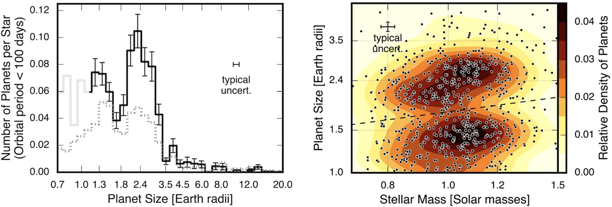
Fig. 19. Left: Radius distribution of short-period transiting exoplanets from the Kepler prime mission. The solid histogram shows the radii of planets in a completeness corrected sample and reveals two populations and a significant gap. The grey curve is planets in regions of poor completeness and the dotted line shows an arbitrarily scaled planet radius distribution prior to completeness corrections. Right: 2D representation of the planet radius distribution revealing that the observed bimodal population and radius gap tend towards smaller planets as host star mass decreases. These observed trends are consistent with irradiation-driven photoevaporative mass-loss being the dominant factor in determining the radius distribution of small, close-in planets. Figure adapted from Fulton and Petigura (Reference Fulton and Petigura2018).
During its K2 mission, Kepler observed multiple fields around the Ecliptic plane that included populations of young stars. These included the Sco-Cen OB association (5–15 Myr), classic young open clusters like the Pleiades (125 Myr), the Hyades (600–800 Myr) and Praesepe (600–800 Myr) and isolated young stars in the Galactic field population (David et al., Reference David, Mamajek, Vanderburg, Schlieder, Bristow, Petigura, Ciardi, Crossfield, Isaacson, Cody, Stauffer, Hillenbrand, Bieryla, Latham, Fulton, Rebull, Beichman, Gonzales, Hirsch, Howard, Vasisht and Ygouf2018 and references therein). These observations yielded the first young transiting exoplanets and this small population revealed an interesting emerging trend: young planets appear anomalously large compared to other planets on short-period orbits transiting older stars of similar mass (David et al., Reference David, Mamajek, Vanderburg, Schlieder, Bristow, Petigura, Ciardi, Crossfield, Isaacson, Cody, Stauffer, Hillenbrand, Bieryla, Latham, Fulton, Rebull, Beichman, Gonzales, Hirsch, Howard, Vasisht and Ygouf2018, see Fig. 20). This trend is most pronounced for young planets transiting low-mass stars which are more active for longer periods of time than their higher mass counterparts. This may be indicative of ongoing, SW-driven radius evolution. In this scenario, photoevaporative mass-loss from host star irradiation is still sculpting the planet's atmosphere and it has not yet reached its final size. At the same time, these young planets may also still be undergoing radius evolution due to core cooling and contraction (Vazan et al., Reference Vazan, Ormel and Dominik2017). Further observations of young stars spread across the sky by the NASA TESS mission will provide more examples of young transiting planets and add to the currently small sample. Detailed study of individual systems and statistical analysis of a larger sample will shed light on this interesting emerging feature in the exoplanet population.
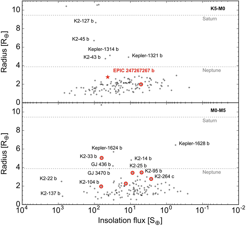
Fig. 20. Insolation flux versus planet radius for known exoplanets transiting sample K5–M5 type host stars (M = 0.7–0.1 M⊙). The flux received by the Earth from the Sun is 1. Young (<1 Gyr) transiting planets discovered by the K2 mission are circled in red. These planets tend to have radii that are larger than planets transiting old stars of similar mass and receiving similar insolation flux. This emerging trend may indicate these young planets are currently undergoing photoevaporative radius evolution. Figure adapted from David et al. (Reference David, Mamajek, Vanderburg, Schlieder, Bristow, Petigura, Ciardi, Crossfield, Isaacson, Cody, Stauffer, Hillenbrand, Bieryla, Latham, Fulton, Rebull, Beichman, Gonzales, Hirsch, Howard, Vasisht and Ygouf2018).
Impact of space weather on (exo)planetary atmospheric chemistry
Effects of SEPs on prebiotic chemistry
As discussed in the section ‘Superflares from active stars’, during the first 500 Myr since its birth, our Sun was a magnetically active star generating a rich variety of high-energy eruptive events that generate ionizing radiation. This radiation in the form of XUV fluxes, CME-driven energetic electrons and protons penetrate various layers of Earth's and Martian atmosphere: from magnetosphere to troposphere (see Fig. 1). Ionizing radiation sources provide three major impacts on atmospheric molecules: photo and particle impact dissociation, excitation and ionization. These processes cause major changes in atmospheric chemistry that in turn control the dosage of ionizing radiation reaching the planetary surfaces, and thus directly affect habitability conditions on rocky planets.
While XUV radiation mostly ionizes the upper atmosphere and contributes to the formation of the Earth's ionosphere and thermosphere (at up to 90 km from the ground), auroral electrons can reach the altitudes of ~80 km, while relativistic electrons penetrate to the mesosphere at 40 km. Solar energetic particles (SEPs) with energies up to a few GeV can precipitate through the troposphere and reach the ground causing GLE events as measured by ground monitors of neutrons, the byproducts of interactions of high-energy protons with atmospheric species (GLEs; see Fig. 21). Impact electrons formed as a result of photo and collisional ionization can then interact with molecular nitrogen, carbon dioxide, methane and water vapour igniting a reactive chemistry in the Earth's lower atmosphere.
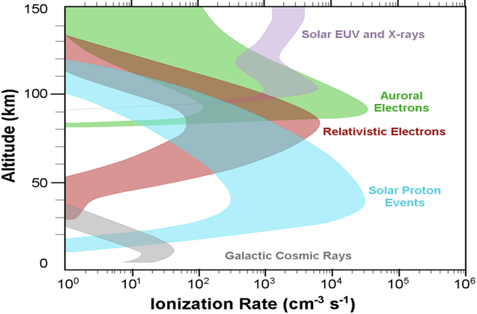
Fig. 21. Ionization of the Earth's atmosphere due to various factors of SW including XUV emission, auroral electrons, SEPs and GCRs.
What would be the effects of such ionizing sources on the atmospheres of early Earth and Mars? Could these sources had been beneficial in starting life on Earth and possibly on Mars? The first clues on the relation between the sources of ionizing radiation and the production of biological molecules were obtained in revolutionary experiments by Miller (Reference Miller1953). In this experiment, a highly reducing gas mixture containing a water vapour, ammonia, NO3, and methane, CH4 and H2 was exposed to a spark discharge. The chemical reactions initiated by the discharge promoted the formation of simple organic molecules including hydrogen cyanide, HCN, formaldehyde and CH2O. These molecules and methane react via Strecker synthesis forming amino acids, the building blocks of proteins (amino acids) and other macromolecules.
However, later studies suggested that the early Earth's atmosphere was weakly reducing consisting of N2, CO2, CO and H2O with only minor abundance of H2, CH4 and H2S (Kasting et al., Reference Kasting, Whitmire and Reynolds1993; Lammer et al., Reference Lammer, Zerkle, Gebauer, Tosi, Noack, Scherf, Pilat-Lohinger, Güdel, Grenfell, Godolt and Nikolaou2018) or neutral (Schaefer and Fegley, Reference Schaefer and Fegley2017). Follow-up experiments showed that non-thermal energy input in the form of lightning (spark discharge between centres of positive and negative charge) in a weakly reducing atmosphere does not efficiently produce abundant amino acids as reported in experiments in highly reducing environments (Cleaves et al., Reference Cleaves, Chalmers, Lazcano, Miller and Bada2008 and references therein). Later, Patel et al. (Reference Patel, Percivalle, Ritson, Duffy and Sutherland2015) presented photochemically driven chemical networks that produce abundant amino acids, nucleosides, the building blocks of RNA and DNA molecules and lipids. Lipids are complex biomolecules that are used to store energy and serve as structural units of cell membranes. Recent experiments suggest that near-UV (NUV at λ = 2000–2800 Å) irradiation of the gas mixture is beneficial factor for formation of building blocks of life (Ranjan and Sasselov, Reference Ranjan and Sasselov2016; Rimmer et al., Reference Rimmer, Xu, Thompson, Gillen, Sutherland and Queloz2018). However, while UV emission promotes biochemical reactions with participation of HCN, it cannot break triple bonds of molecular nitrogen, N2, that require 10 eV to create odd nitrogen (N), which is required to produce abundant HCN, the requirement for the chemical network by Patel et al. (Reference Patel, Percivalle, Ritson, Duffy and Sutherland2015).
HCN is the most important feedstock molecule for prebiotic chemistry that is the crucial for formation of amino acids, nucleobases and complex sugars. In order to produce HCN and other biologically important molecules, molecular nitrogen needs to be converted into odd nitrogen and follow-up NOx (NO, NO2) molecules, the process known as the nitrogen fixation. In order to efficiently precipitate these molecules down to the ground for further polymerization, the nitrogen fixation and subsequent production of HCN should occur in the lower atmosphere (stratosphere–troposphere layers) of Earth (Airapetian et al., Reference Airapetian, Glocer, Gronoff, Hébrard and Danchi2016). This is an important requirement for the efficient delivery of HCN to the ground for subsequent synthesis into complex molecules (Airapetian et al., Reference Airapetian, Glocer, Gronoff, Hébrard and Danchi2016).
The nitrogen fixation process can be achieved in the lower atmosphere either by high-energy processes including extremely high temperatures (a few tens of thousands of Kelvins) that can be reached by atmospheric shock heating from impact processes, due to lightning processes that produce HEEs or solar EUV radiation with wavelengths shorter than 100 nm (Kasting, Reference Kasting1990; Summers et al., Reference Summers, Basa, Khare and Rodoni2012). Asteroid and comet impacts with Earth involve collisions with impact velocities from 20 to 70 km s−1. Such impact events heat the atmosphere and the ground to a few times of 104 Kelvin. An impactor can create the favourable conditions for synthesis of reducing gas mixtures and form biologically relevant molecules (Chyba and Sagan, Reference Chyba and Sagan1992). Also, large molecules contained in the impactors can survive high-velocity impacts and be delivered to the planetary surface (Pierazzo and Chyba, Reference Pierazzo and Chyba1999). These macromolecules can be dissolved into the ‘primordial’ soup to provide further polymerization. However, the resulted concentration required to produce peptides, ribose, fatty acids, nucleobases, ribose and oligonucleotides through polymerization has not been discussed in detail. EUV emission is another factor for nitrogen fixation, but it is absorbed at altitudes above 90 km above the ground (see Fig. 21), and thus can provide significant amount of atomic hydrogen and other dissociated molecules required for the production of HCN in the upper atmosphere (Tian et al., Reference Tian, Kasting and Zahnle2011). However, the problem of efficient delivery of HCN to the lower atmosphere is problematic because of a slow vertical diffusion throughout the atmosphere. The alternative energy source, energetic particles from GCRs or SEP events can provide a mechanism to deliver the particles directly to the lower atmosphere. The penetration depth depends on the frequency of collisions of protons with ambient molecules and for the Earth's atmosphere is scaled with the proton's energy as E −1.72 (Jackman et al., Reference Jackman, Frederick and Stolarski1980). This suggests that the protons with energy of 300 MeV can penetrate to the heights of 4.5 km above the ground. The collisions with molecules produce enhanced ionization of the atmosphere and form a broad energy distribution of secondary electrons at >35 eV. These electrons then thermalize to lower energies in the atmosphere and as soon their energy reaches 10 eV, they become very efficient in breaking N2 into odd nitrogen with subsequent formation of NOx. To study the pathways to complex organic molecules driven by energetic protons, Kobayashi et al. (Reference Kobayashi, Tsuchiya, Oshima and Yanagawa1990, Reference Kobayashi, Kaneko, Saito and Oshima1998, Reference Kobayashi, Shibata, Fukuda, Oguri, Kebukawa, Aoki, Kinoshita, Kunwar, Kawamura and Airapetian2018) and Miyakawa et al. (Reference Miyakawa, James and Miller2002) have performed laboratory experiments exposing gas mixtures of CO/CO2, CO, N2 and H2O to 2.5 MeV protons. They reported production of amino acids precursors and nucleic acid bases as the results of secondary electron-driven reactive chemistry. These experiments may have a direct relevance to the early Earth's atmospheric chemistry as high-energy protons from SEP events precipitated through the Archaean Earth's atmosphere causing showers as a result of impact ionization. As discussed in the section ‘Winds from active stars’, the young Sun was a source of frequent and energetic flares and associated CMEs. The CME-driven shocks are the sites of efficient accelerations of SEPs that can accelerate particles to high energies (Fu et al., Reference Fu, Jiang, Vladimir Airapetian, Hu, Li and Zank2019). To study the role of SEPs from the young Sun as the source of high-energy protons in gas phase prebiotic chemistry in the atmosphere of early Earth, Airapetian et al. (Reference Airapetian, Glocer, Gronoff, Hébrard and Danchi2016) have applied a photo-collisional atmospheric chemistry model driven by the XUV flux and frequent SEP events. SEP-driven protons with energies >0.3 GeV (at 0.5 bar atmosphere) precipitate into the middle and lower atmosphere (stratosphere and troposphere) and produce enhanced ionization, dissociation, dissociative ionization and excitation of atmospheric species. The destruction of N2 into ground state atomic nitrogen, N(4S) and the excited state of atomic nitrogen, N(2D), as the first key step towards production of bio-relevant molecules. Reactions of these species with the products of subsequent dissociation of CO2, CH4 and H2O produces nitrogen oxides, NOx, CO and NH in the polar regions of the atmosphere. NOx then converts in the stratosphere into HNO2, HNO3 and its products including nitrates and ammonia.
The atmospheric model also predicts an efficient production of nitrous oxide, N2O, driven primarily through N(4S) + NO2 → N2O + O; NO + NH → N2O + H. The recent model updated with the hard energy spectrum of protons, vertical diffusion and Rayleigh scattering outputs the N2O production in the lower atmosphere by a factor >300 greater than the earlier model output of Airapetian et al. (Reference Airapetian, Glocer, Gronoff, Hébrard and Danchi2016). This is due to the fact that the CME-driven shocks in the young Sun's corona, the source of CMEs, was at least a factor of 10 denser compared to the current Sun. Denser corona provided correspondingly larger concentrations of seed particles, while stronger shocks (larger compression ratio) produce SEPs with higher maximum energy and harder proton energy slopes. The particle acceleration via diffusive shock acceleration mechanisms on quasi-parallel strong shocks produces mostly SEPs with harder spectra (Fu et al., Reference Fu, O'Connell and Sasselov2010). This is consistent with the recent statistical study of CME-driven SEPs with hard energy spectra by Gopalswamy et al. (Reference Gopalswamy, Yashiro and Akiyama2016) and suggests the particle flux at 0.5–1 GeV is over 2 orders of magnitude greater than that assumed in the atmospheric chemistry model by Airapetian (Reference Airapetian2018a) (see Fig. 18).
Laboratory experiments suggest that SEP-driven chemistry predicts much more efficient production of HCN than that produced by lightning events for a weakly reducing (N2–CO/CO2–CH4–H2O) atmosphere on early Earth (Kobayashi et al., Reference Kobayashi, Kaneko, Saito and Oshima1998, Reference Kobayashi, Shibata, Fukuda, Oguri, Kebukawa, Aoki, Kinoshita, Kunwar, Kawamura and Airapetian2018; Takano et al., Reference Takano, Kaneko, Kobayashi, Hiroishi, Ikeda and Marumo2004). HCN is formed primarily due to neutral reactions including NO + CH → HCN + O, CH2 + N(4S) → HCN + H, CH3 + N(4S) → HCN + H + H and CH + CN → HCN + H. As it forms in the stratosphere–troposphere region, HCN may subsequently rain out into surface reservoirs and initiate higher order chemistry producing more complex organics. For example, the hydrolysis of HCN through reactions with water cloud droplets produces formamide, HCONH2, that can rain out to the surface. Formamide serves as an important precursor of complex biomolecules that are capable of producing amino acids, the building blocks of proteins and nucleobases, sugars and nucleotides, the constituents of RNA and DNA molecules (Saladino et al., Reference Saladino, Carota, Botta, Kapralov, Timoshenko, Rozanov, Krasavin and Di Mauro2015; Hud, Reference Hud2018).
This scenario has recently been studied under lab conditions by Kobayashi et al. (Reference Kobayashi, Aoki, Kebukawa, Shibata, Fukuda, Oguri and Airapetian2017, Reference Kobayashi, Shibata, Fukuda, Oguri, Kebukawa, Aoki, Kinoshita, Kunwar, Kawamura and Airapetian2018), who performed a series of prebiotic chemistry experiments to study the formation of amino acids by irradiating weakly reducing gas mixtures (N2–CO2–CH4–H2O) that resemble a weakly reducing early Archaean Earth's atmosphere with ionizing sources to simulate the energy flux from galactic and SEPs, UV emission and spark discharge (lightning) radiation. In these experiments, alanine and glycine were detected when gas mixtures with CH4 molar ratio (r CH4) as low as 0.5% was irradiated by energetic protons with an energy range of 2.5–4 MeV generated from a van de Graaff accelerator (Tokyo Institute of Technology). The maximum G-value (the production rate in units of number of amino acid molecules per eV) for glycine is reached at r CH4 = 5%. However, when the same mixture was exposed to irradiation by the spark discharge (accelerated electrons) or UV irradiation, amino acids were not detected for r CH4 lower than 15%. Considering fluxes of various energies on the primitive Earth (Kobayashi et al., Reference Kobayashi, Kaneko, Saito and Oshima1998), energetic protons appear to be more efficient factor to produce N-containing organics than any other conventional energy sources like lightning or solar UV emission which irradiated the early Earth atmosphere.
Nitrous oxide, N2O, is another abundant molecule produced by the chemical reaction network driven by SEP in the early Earth's atmosphere (see Fig. 22). This molecule is a potent greenhouse gas, 300 times stronger in greenhouse power than CO2 and is currently present in Earth's atmosphere produced at ~400 ppbv via biological processes. While its atmospheric concentration 1000 times less than CO2, it contributes ~6% to the global warming of our planet. Airapetian et al. (Reference Airapetian, Danchi, Dong, Rugheimer, Mlynczak, Stevenson, Henning, Grenfell, Jin, Glocer, Gronoff, Lynch, Johnstone, Lueftinger, Guedel, Kobayashi, Fahrenbach, Hallinan, Stamenkovic, Cohen, Kuang, van der Holst, Manchester, Zank, Verkhoglyadova, Sojka, Maehara, Notsu, Yamashiki, France, Lopez Puertas, Funke, Jackman, Kay, Leisawitz and Alexander2018a) have recently applied the results of Fig. 22 as input for climate model to show that the annually mean temperature of late Hadean Earth can be ~5.2°C. This is important to resolve a longstanding problem known as the Faint Young Sun (FYS) paradox (see a review by Feulner, Reference Feulner2012). The young Sun was under late Hadean Earth was ~25% fainter that it is today, which will be insufficient to support liquid water on the early Earth contrary to geological evidence of its presence that time (Sagan and Mullen, Reference Sagan and Mullen1972; Feulner, Reference Feulner2012). Further theoretical and experimental efforts are needed to study the pathways and the products of the SEP and XUV modified gas phase chemistry to form ‘exotic’ greenhouse molecules. Nitrous oxide may provide strong spectral signatures in the upcoming observational efforts to study signatures of life and also be instrumental in resolving the FYS for early Earth and Mars.
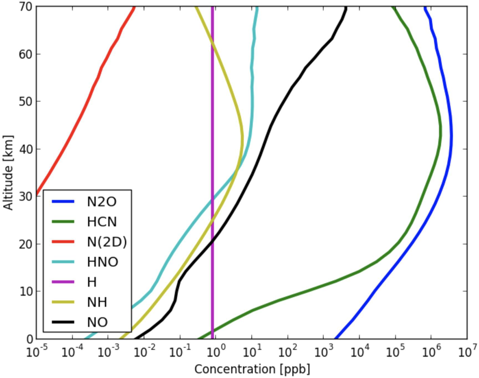
Fig. 22. Steady-state concentrations of molecules produced via photo-collisional chemistry from precipitating high-energy protons in the atmosphere of early Earth (Airapetian, Reference Airapetian2018a).
Impact of SEPs on surface dosages of ionizing radiation
SEPs induced by strong stellar CMEs may have a significant impact not only on the atmospheric chemistry, but also on the surface dosage of ionizing radiation that may affect surface habitability of terrestrial-type exoplanets. Recent modelling of SEP-driven ionizing radiation in the atmospheres of exoplanets around M dwarfs of different chemical compositions and atmospheric pressures including Proxima-b and TRAPPIST-1 suggest that impact on life forms at 1 bar atmospheric pressure is relatively small compared to the critical dose at 10 Sv (Atri, Reference Atri2017; Yamashiki et al., Reference Yamashiki, Maehara, Airapetian, Notsu, Sato, Notsu, Kuroki, Murashima, Sato, Namekata, Sasaki, Scott, Bando, Nashimoto, Takagi, Ling, Nogami and Shibata2019 and also shown in Fig. 23). Considering that exoplanetary atmospheres may suffer severe atmospheric escape in proportion to the XUV flux from their host stars (Airapetian et al., Reference Airapetian, Jackman, Mlynczak, Danchi and Hunt2017b, see Fig. 17), the surface environment for the majority of exoplanets in the CHZs around M dwarfs may become inhospitable at least for complex terrestrial-type life forms (see Fig. 23).

Fig. 23. (a) Vertical profile of radiation dose (in Gy) and (b) (in Sv), caused by hard proton spectrum imitating GLE 43 penetrating N2 + H2 rich terrestrial-type atmosphere of TRAPPIST-1b (blue square), c (red cross), d (green square), e (blue circle), f (black square), g (blue cross) and h (red square) in the logarithmic scale under Annual Maximum flare energy, calculating using PHITS (Sato et al., Reference Sato2015) and ExoKyoto. Vertical red dotted line represents Martian equivalent atmospheric depth, pink dotted line represents the depth 0.1 bar atmosphere, blue dotted line represents lowest terrestrial atmospheric depth observed at the summit of Himalaya and blue dotted line as terrestrial atmospheric depth. Horizontal blue dotted line represents 10 Sv, which may be considered as critical dose for complex terrestrial-type lifeform. Figure adapted from Yamashiki et al. (Reference Yamashiki, Maehara, Airapetian, Notsu, Sato, Notsu, Kuroki, Murashima, Sato, Namekata, Sasaki, Scott, Bando, Nashimoto, Takagi, Ling, Nogami and Shibata2019).
Space weather, habitability and biosignatures
‘Habitability’ broadly refers to conditions which can sustain life. An unequivocable definition of life itself remains elusive although often-quoted is the ‘self-sustaining chemical system capable of Darwinian evolution’ (Joyce et al., Reference Joyce1994). Life as we know it has three essential requirements, namely (i) an energy source, (ii) liquid water and (iii) the chemical elements CHNOPS (see e.g. Cockell et al., Reference Cockell, Bush, Bryce, Direito, Fox-Powell, Harrison, Lammer, Landenmark, Martin-Torres, Nicholson, Noack, O'Malley-James, Payler, Rushby, Samuels, Schwendner, Wadsworth and Zorzano2016). The classical CHZ refers to the circular region around a star where a terrestrial planet can support liquid water (Huang, Reference Huang1960; Kasting et al., Reference Kasting, Whitmire and Reynolds1993). An empirically-defined ‘conservative habitable zone’ has also been introduced, with limits based on evidence that recent Venus and early Mars may have had conditions permitting liquid water on their surfaces (Kasting et al., Reference Kasting, Kopparapu, Ramirez and Harman2014). The continuous HZ (e.g. Hart, Reference Hart1979) refers to the circular region around a star, which remains potentially habitable changes in stellar luminosity over geological time. Its inner and outer boundaries depend on stellar mass and metallicity, because they strongly affect the stellar luminosity and effective temperature (Gallet and Bouvier, Reference Gallet and Bouvier2013).
The non-classical HZ extends beyond the snowline and includes objects proposed to have subsurface oceans (Lammer et al., Reference Lammer, Bredehöft, Coustenis, Khodachenko, Kaltenegger, Grasset, Prieur, Raulin, Ehrenfreund, Yamauchi, Wahlund, Grießmeier, Stangl, Cockell, Kulikov, Grenfell and Rauer2009). Other phenomena proposed to affect habitability include e.g. the output of the central star (Beech, Reference Beech2011); the planetary atmospheric mass and composition (e.g. Grenfell et al., Reference Grenfell, Rauer, Selsis, Rauer, Selsis, Kaltenegger, Beichman, Danchi, Eiroa, Fridlund, Henning, Herbst, Lammer, Léger, Liseau, Lunine, Paresce, Penny, Quirrenbach, Röttgering, Schneider, Stam, Tinetti and White2010); the presence of stabilizing climate feedbacks driven by e.g. plate tectonics (Korenaga, Reference Korenaga2013); the presence of a large moon (Laskar et al., Reference Laskar, Joutel and Robutel1993); planetary orbital parameters such as the rotational rate (e.g. Del Genio and Zhou, Reference Del Genio and Zhou1996; Edson et al., Reference Edson, Lee, Bannon, Kasting and Pollard2011; Yang et al., Reference Yang, Liu, Hu and Abbot2014) and the role of the planetary magnetosphere (e.g. Shizgal and Arkos, Reference Shizgal and Arkos1996).
There are numerous ways in which SW from planet hosts could influence habitability conditions within CHZs – for example lower mass main sequence stars have stronger magnetic fields and lager XUV fluxes which may impact exoplanetary magnetospheric and atmospheric erosion, two critical factors affecting surface climate and radiation as well as surface radiation doses as discussed in the section ‘Impact of space weather on (exo)planetary atmospheric chemistry’.
Atmospheric models of habitable environments
A major goal of this section is to discuss the factors necessary for habitability and the extent of habitable environments in the Universe. These clearly have repercussions for the distribution of potential life and biosignatures which drives the design of next generation exoplanetary missions. A central task is to constrain the HZ for a given planetary system by applying numerical models. Earlier 1D model studies (e.g. Hart, Reference Hart1979) suggested a thin HZ for Sun-like stars extending from 0.95 to 1.01 Astronomical Units (AU). Subsequent studies (e.g. Kasting et al., Reference Kasting, Toon and Pollack1988) however, noted that including atmospheric climate feedbacks such as the carbonate–silicate cycle (Walker et al., Reference Walker, Hays and Kasting1981) could considerably widen the HZ.
Regarding the habitability of the early Earth, there exists a discrepancy between ancient soil (paleosol) data and the output of certain atmospheric climate-column models which suggests a frozen surface. Briefly, proposed solutions for the FYS paradox include e.g. (i) an increased abundance of greenhouse gases such as methane (CH4(g)) (Pavlov et al., Reference Pavlov, Hurtgen, Kasting and Arthur2003) and/or nitrous oxide (N2O(g)) (Grenfell et al., Reference Grenfell, Gebauer, von Paris, Godolt and Hedelt2011; Roberson et al., Reference Roberson, Roadt, Halevy and Kasting2011), (ii) enhanced line-broadening by molecular nitrogen (N2) (Goldblatt et al., Reference Goldblatt, Claire, Lenton, Matthews, Watson and Zahnle2009), (iii) increased planetary albedo (Rosing et al., Reference Rosing, Bird, Sleep and Bjerrum2010) due to a lowering in biogenic cloud precursors or (iv) updated carbon dioxide (CO2) thermal absorption coefficients (von Paris et al., Reference von Paris, Rauer, Lee Grenfell, Patzer, Hedelt, Stracke, Trautmann and Schreier2008). 3D model studies addressing the FYS problem (Charnay et al., Reference Charnay, Forget, Wordsworth, Leconte, Millour, Codron and Spiga2013; Wolf and Toon, Reference Wolf and Toon2013; Kunze et al., Reference Kunze, Godolt, Langematz, Grenfell, Hamann-Reinus and Rauer2014) noted that tropical latitudes could remain habitable even if the global mean surface temperature lies below the freezing point. Organic photochemical hazes that can form in reducing atmospheres with sufficiently high CH4 concentrations had been thought to be an obstacle to keeping Archaean Earth warm enough to sustain liquid water (Sagan and Chyba, Reference Sagan and Chyba1997). More recent work suggests however that the fractal nature of such hazes (Wolf and Toon, Reference Wolf and Toon2010) and self-shielding effects (Arney et al., Reference Arney, Domagal-Goldman, Meadows, Wolf, Schwieterman, Charnay, Claire, Hébrard and Trainer2016) limit the surface cooling that can occur in the visible portion of the FYS spectrum while blocking harmful radiation in the UV.
For the inner HZ there are two boundaries. Firstly, the ‘water-loss’ (or ‘moist greenhouse’ limit’) (Kasting, Reference Jeans1988) occurs where the planet's entire ocean reservoir is lost via diffusion-limited escape within the lifetime of the planet (originally estimated to occur at = 0.95 AU for Earth (Kasting et al., Reference Kasting, Whitmire and Reynolds1993) and more recently at 0.99 AU (Kopparapu et al., Reference Kopparapu, Ramirez, Kasting, Eymet, Robinson, Mahadevan, Terrien, Domagal-Goldman, Meadows and Deshpande2013) for 1D cloud-free models and main-sequence stars). Secondly, the ‘runaway greenhouse limit’ occurs where the surface temperature reaches the critical point of water (T c = 647 K) (=0.84 AU for Earth (Kasting et al., Reference Kasting, Toon and Pollack1988); see also Wolf and Toon, Reference Wolf and Toon2015). Recent 1D model studies (e.g. Kasting et al., Reference Kasting, Kopparapu, Ramirez and Harman2014) noted the challenge of performing accurate climate transfer calculations in thick steam atmospheres near the inner HZ boundary. The 1D study of Zsom et al. (Reference Zsom, Seager, de Wit and Stamenković2013) suggested a very close ( = 0.38 AU) inner HZ boundary for a desert world with high-surface albedo (A = 0.8) and low relative humidity (RH = 1%) orbiting a solar-mass main sequence star. 3D model studies near the HZ boundary suggest e.g. climate-cloud feedbacks (Yang et al., Reference Yang, Cowan and Abbot2013) and massive atmospheric circulation (e.g. Hadley cell) responses (Leconte et al., Reference Leconte, Forget, Charnay, Wordsworth and Pottier2013a, Reference Leconte, Forget, Charnay, Wordsworth, Selsis, Millour and Spiga2013b) which suggest an expansion of the inner HZ boundary towards the star. Yang et al. (Reference Yang, Liu, Hu and Abbot2014) suggest a strong dependence of the inner HZ position upon planetary rotation rate associated with an atmospheric dynamical response driven by changes in the Coriolis force. A recent 3D model study (Kopparapu et al., Reference Kopparapu, Wolf, Haqq-Misra, Yang, Kasting, Meadows, Terrien and Mahadevan2016) suggested a modest revision of the inner HZ boundary inwards on including consistent planetary rotation due to tidal-locking and associated cloud effects.
For the outer HZ, the ‘maximum greenhouse limit’ ( = 1.67 AU for Earth (Kasting et al., Reference Kasting, Whitmire and Reynolds1993) occurs where greenhouse warming of the planetary surface from carbon dioxide (CO2(g)) is strongest. Increasing the abundance of atmospheric CO2(g) above this limit leads to a net cooling of the surface due to enhanced Rayleigh scattering. The CO2(g) abundance and its ability to stabilize climate depends upon outgassing rates from the interior and whether the planet features plate tectonics (see also section ‘Impact of space weather effects on modern Earth, Venus and Mars’). Pierrehumbert and Gaidos (Reference Pierrehumbert and Gaidos2011a, Reference Pierrehumbert and Gaidos2011b) suggested that collision-induced absorption from hydrogen (H2) atmospheres could extend the outer HZ to as far as 10 AU for planets orbiting a sun-like star, even though planets would lose their H2 inventories within a few million years. Ramirez and Kaltenegger (Reference Ramirez and Kaltenegger2017) have recently proposed that the CO2–H2O CHZ (e.g. Kasting et al., Reference Kasting, Whitmire and Reynolds1993) could be significantly widened on planets with volcanoes that outgassed significant amounts of H2, which moves the outer edge limit outwards (from 1.67 to ~2.4 AU in our Solar System). A recent 3D model study (Wolf, Reference Wolf2017) suggests that the 1D outer edge maximum greenhouse limit (1.67 AU) may not actually be realizable because of the high cloud and surface albedos of cold planets and subsaturation of water vapour. The extra warming from H2 could partially offset this problem though (Ramirez and Kaltenegger, Reference Ramirez and Kaltenegger2017). On the other hand, even for an Earth-like atmospheric composition, habitability may be possible for colder surface temperatures if the ocean is more saline than Earth's (Cullum et al., Reference Cullum, Stevens and Josh2016; Del Genio et al., Reference Del Genio, Way and Amundsen2017).
Habitability of Earth-like planets orbiting M-dwarf stars
Rocky planets orbiting in the HZ of M-dwarf stars are on the one hand favoured objects for next-generation mission surveys since such stars are numerous in the solar neighbourhood, their planets have high (planet/star) contrast ratios and the close proximity of HZ planets to the central star means more frequent transit events and hence faster data collection over a given observing interval. On the other hand, such planets have potential drawbacks with regards to their potential habitability as reviewed in Scalo et al. (Reference Scalo, Kaltenegger, Segura, Fridlund, Ribas, Kulikov, Grenfell, Rauer, Odert, Leitzinger, Selsis, Khodachenko, Eiroa, Kasting and Lammer2007) and Shields et al. (Reference Shields, Ballard and Johnson2016). Firstly, the close proximity of the HZ to the central star could most likely lead to HZ planets becoming tidally-locked i.e. where strong gravitational interaction leads to the possibility of synchronous rotation (the planet having a constant day and night side). Whether the planet's surface remains habitable then depends on the ability of its atmosphere to transport heat from the dayside to the nightside. In practice, numerous 3D model studies have indicated that this is not an obstacle to habitability of the dayside region as long as (1) there is sufficient water to create an optically thick dayside convective cloud deck that shields the surface from direct starlight (e.g. Yang et al., Reference Yang, Cowan and Abbot2013; Kopparapu et al., Reference Kopparapu, Wolf, Haqq-Misra, Yang, Kasting, Meadows, Terrien and Mahadevan2016; Turbet et al., Reference Turbet, Leconte, Selsis, Bolmont, Forget, Ribas, Raymond and Anglada-Escudé2016; Boutle et al., Reference Boutle, Mayne, Drummond, Manners, Goyal, Lambert, Acreman and Earnshaw2017; Wolf, Reference Wolf2017) and (2) the land–ocean configuration prevents water from being completely trapped as ice on the nightside (Yang et al., Reference Yang, Liu, Hu and Abbot2014). Nonetheless, the ‘moist greenhouse’ habitability limit of diffusion-limited escape occurs at lower instellation values for cooler stars because of their reducing Rayleigh scattering and predominantly near-infrared incident stellar flux, the latter which is strongly absorbed by water vapour, driving a stratospheric circulation that transports significant H2O to high altitudes where it is readily dissociated (e.g. Kasting et al., Reference Kasting, Whitmire and Reynolds1993; Fujii et al., Reference Fujii, Angerhausen, Deitrick, Domagal-Goldman, Grenfell, Hori, Kane, Palle, Rauer, Siegler, Stapelfeldt and Stevenson2017; Kopparapu et al., Reference Kopparapu, Wolf, Arney, Batalha, Haqq-Misra, Grimm and Heng2017).
Other factors that influence the habitability of M-star planets involve the evolutionary phase of bolometric luminosity and magnetic activity of host stars, their impact on a planet and internal planetary dynamics. For some planets, the luminous pre-main sequence phase of the host star may have driven the planet into a runaway greenhouse state before it had a chance to become habitable (Ramirez and Kaltenegger, Reference Ramirez and Kaltenegger2014; Luger and Barnes, Reference Luger and Barnes2015; Bolmont et al., Reference Bolmont, Selsis, Owen, Ribas, Raymond, Leconte and Gillon2017) although worlds located in the pre-main-sequence HZ may be habitable (Ramirez and Kaltenegger, Reference Ramirez and Kaltenegger2014). For others, conditions in the protoplanetary disc may have worked in favour of or against habitability, e.g. variations in water delivery to planets (Tian and Ida, Reference Tian and Ida2015; Ribas et al., Reference Ribas, Bolmont, Selsis, Reiners, Leconte, Raymond, Engle, Guinan, Morin, Turbet, Forget and Anglada-Escudé2016) and an H2-poor versus H2-rich nebula that may have provided initial shielding planetary envelopes of different thicknesses to protect Earth-size planetary cores and their atmospheres from complete photoevaporation (Luger et al., Reference Luger, Barnes, Lopez, Fortney, Jackson and Meadows2015). The California-Kepler survey suggests at least a small number of planets of a size that would be consistent with a remnant thin H2 envelope (Fulton et al., Reference Fulton, Petigura, Howard, Isaacson, Marcy, Cargile, Hebb, Weiss, Johnson, Morton, Sinukoff, Crossfield and Hirsch2017). The composition of the planet, to the extent that it is related to elemental abundances for its host star, may determine its interior structure (Dorn et al., Reference Dorn, Rozel and Noack2017) and influence the tectonic history of the planet and thus the coupling of its climate to the interior (Lenardic et al., Reference Lenardic, Jellinek, Foley, O'Neill and Moore2016). Finally, due (a) to the close proximity of the planet to the star and (b) (possible) weakening of the magnetospheric field (if present) due to tidal-locking – the stellar environment could lead to strong bombardment of the atmosphere with high-energy particles and UV that either strip the planet of its atmosphere or leave its surface inhospitable to life (see also section ‘Space weather impact on (exo)planetary systems: atmospheric loss’).
Atmospheric biosignatures
The term biosignature refers here to evidence which suggests the presence of biological forms of life. The subject is broad, spanning a range of disciplines (e.g. biology, geology, atmospheric science) and physical criteria (e.g. fossil morphology, isotope signatures, chiral signals, departures from thermodynamic and redox equilibria, presence of gas-phase species, etc.). Broadly speaking, an ‘ideal’ biosignature should be (i) easily detectable with a large signal-to-noise ratio, (ii) unequivocally biological i.e. without abiotic sources and (iii) easily retrievable from the data without e.g. data degeneracies, numerical issues, etc.
The topic may be broadly split into two parts, namely in-situ and remote biosignatures. In this paper, we focus on remote biosignatures via spectroscopic detection of atmospheric species in an exoplanet context. We discuss thereby possible abiotic production mechanisms (in order to rule out false signals from non-life), biosignature detectability and the role of SW. A series of five comprehensive review papers in biosignature science (Fujii et al., Reference Fujii, Angerhausen, Deitrick, Domagal-Goldman, Grenfell, Hori, Kane, Palle, Rauer, Siegler, Stapelfeldt and Stevenson2017; Walker et al., Reference Walker, Bains, Cronin, DasSarma, Danielache, Domagal-Goldman, Kacar, Kiang, Lenardic, Reinhard, Moore, Schwieterman, Shkolnik and Smith2018; Catling et al., Reference Catling, Krissansen-Totton, Kiang, Crisp, Robinson, DasSarma, Rushby, Del Genio, Bains and Domagal-Goldman2018; Meadows et al., Reference Meadows, Reinhard, Arney, Parenteau, Schwieterman, Domagal-Goldman, Lincowski, Stapelfeldt, Rauer, DasSarma, Hegde, Narita, Deitrick, Lustig-Yaeger, Lyons, Siegler and Grenfell2018b; Schwieterman et al., Reference Schwieterman, Kiang, Parenteau, Harman, DasSarma, Fisher, Arney, Hartnett, Reinhard, Olson, Meadows, Cockell, Walker, Grenfell, Hegde, Rugheimer, Hu and Lyons2018) organized by the NASA research network NExSS (Nexus for Exoplanet System Science) emphasized the following key points: (1) remote biosignatures need to be interpreted in their full environmental context i.e. combined with information on stellar input, planetary evolution, etc. (Airapetian et al., Reference Airapetian, Danchi, Dong, Rugheimer, Mlynczak, Stevenson, Henning, Grenfell, Jin, Glocer, Gronoff, Lynch, Johnstone, Lueftinger, Guedel, Kobayashi, Fahrenbach, Hallinan, Stamenkovic, Cohen, Kuang, van der Holst, Manchester, Zank, Verkhoglyadova, Sojka, Maehara, Notsu, Yamashiki, France, Lopez Puertas, Funke, Jackman, Kay, Leisawitz and Alexander2018a, Reference Airapetian, Adibekyan, Ansdell, Cohen, Cuntz, Danchi, Dong, Drake, Fahrenbach, France, Garcia-Sage, Glocer, Grenfell, Gronoff, Hartnett, Henning, Hinkel, Jensen, Jin, Kalas, Kane, Kobayashi, Kopparapu, Leake, López-Puertas, Lueftinger, Lynch, Lyra, Mandell, Mandt, Moore, Nna-Mvondo, Notsu, Maehara, Yamashiki, Shibata, Oman, Osten, Pavlov, Ramirez, Rugheimer, Schlieder, Schnittman, Shock, Sousa-Silva, Way, Yang, Young and Zank2018b; Meadows et al., Reference Meadows, Reinhard, Arney, Parenteau, Schwieterman, Domagal-Goldman, Lincowski, Stapelfeldt, Rauer, DasSarma, Hegde, Narita, Deitrick, Lustig-Yaeger, Lyons, Siegler and Grenfell2018b); (2) exo-atmospheric biosignature science has recently developed a much more mature understanding of potential abiotic sources, especially for O2(g) (see Grenfell (Reference Grenfell2017) for a review of the response of atmospheric biosignatures in an exoplanet context) and (3) given the observational challenges for biosignature detection and the open-ended nature of potential theories for false positives, a probabilistic approach to claims of biosignature detection will be necessary.
Impact of stellar UV emission on biosignatures
The seminal study by Des Marais et al. (Reference Des Marais, Harwit, Jucks, Kasting, Lin, Lunine, Schneider, Seager, Traub and Woolf2002) investigated spectral detection of atmospheric biosignatures such as O2 and O3 on Earth-like worlds. Several studies (e.g. Segura et al., Reference Segura, Krelove, Kasting, Sommerlatt, Meadows, Crisp, Cohen and Mlawer2003; Grenfell et al., Reference Grenfell, Stracke, von Paris, Patzer, Titz, Segura and Rauer2007, Reference Grenfell, Gebauer, v. Paris, Godolt and Rauer2014; Kaltenegger et al., Reference Kaltenegger, Traub and Jucks2007; Rugheimer et al., Reference Rugheimer, Kaltenegger, Zsom, Segura and Sasselov2013, Reference Rugheimer, Kaltenegger, Segura, Linsky and Mohanty2015) subsequently modelled the effect of the incoming stellar radiation (in particular UV) upon Earth-like planets orbiting in the HZ of different spectral classes. They found that electromagnetic radiation from the central star could play an important role in atmospheric climate, photochemistry and planetary spectral signals.
Regarding planets in the HZ of M-dwarfs, Segura et al. (Reference Segura, Kasting, Meadows, Cohen, Scalo, Crisp, Butler and Tinetti2005) modelled the effect of UV suggesting that biosignatures such as N2O(g) and CH3Cl(g) could build-up by 2–3 orders of magnitude compared with the modern Earth. Segura et al. (Reference Segura, Walkowicz, Meadows, Kasting and Hawley2010) modelled the UV (and the high-energy particle) effect of a stellar flare upon the atmospheric habitability for a hypothetical Earth-like planet orbiting in the HZ of the M-dwarf star AD Leo. Results suggested that flares may not present a direct hazard to potential life. Rauer et al. (Reference Rauer, Gebauer, Paris, Cabrera, Godolt, Grenfell, Belu, Selsis, Hedelt and Schreier2011), Grenfell et al. (Reference Grenfell, Gebauer, Godolt, Palczynski, Rauer, Stock, von Paris, Lehmann and Selsis2013) and Rugheimer et al. (Reference Rugheimer, Kaltenegger, Segura, Linsky and Mohanty2015) noted that changing the spectral class and activity (hence UV output) of the central M-dwarf star could have a potentially large effect upon atmospheric biosignature abundance and spectral signal. Because XUV flux may cause atmospheric erosion especially on exoplanets in HZs around M dwarfs, atmospheric pressure should be significantly lower than that assumed in these models unless a planet hosting star is magnetically quiet and planet is volcanically active to replenish high rates of escape (Airapetian et al., Reference Airapetian, Glocer, Khazanov, Loyd, ROP, France, K, Sojka, J, Danchi, WC and Liemohn, MW2017a; Garcia-Sage et al., Reference Garcia-Sage, Glocer, Drake, Gronoff and Cohen2017).
While oxygen (O2), its photochemical product, ozone (O3); methane (CH4), nitrous oxide (N2O) have been proposed as gas-phase biosignatures, they cannot be considered robust in isolation due to the known abiotic production mechanisms for O2, O3, CH4 and N2O. A combination of biosignatures and an understanding of the planetary context will be required to claim a planet has a high potential of having life. Chloromethane (CH3Cl) is another proposed biosignature that has no known false positive mechanisms and it is a highly specific molecule unlikely to be produced in large quantities on an exoplanet if at all (see Seager et al., Reference Seager, Bains and Hu2013a for a discussion on types of biosignatures). Seager et al. (Reference Seager, Bains and Hu2013b) also suggested NH3 as a potential biosignature in a temperate, H2 dominated world. NH3 has a short atmospheric lifetime on Earth as it is easily photolysed by UV radiation. Ozone plays an additional role because its fate could be intermingled with those of the other species. This is because loss of the protective ozone layer on an Earth-like planet would likely result in a flooding of UV photons into the lower atmosphere which would strongly increase the photochemical removal of the other biosignatures, CH4, N2O and CH3Cl.
Regarding the effect of UV, ozone is on the one hand produced via molecular oxygen photolysis in the Herzberg region (λ < 242 nm) – producing oxygen atoms (O) which quickly react with O2 to form O3. On the other hand, ozone is photolytically destroyed at wavelengths ranging from ~242 to 320 nm. This implies a dependence of ozone abundance to UV with a ‘switchover’ regime from ozone loss to ozone production with decreasing (UV) wavelength. The response of ozone to UV is further complicated by so-called catalytic cycles involving HOx, NOx and ClOx (as discussed in the section ‘Drivers and signatures of space weather from the Sun’) which remove ozone from the middle atmosphere. The effect of increasing UV generally favours stronger catalytic loss, because it favours the release of HOx, NOx and ClOx from their so-called reservoir (inert) species. For example, nitric acid (HNO3) is a reservoir of both HOx and NOx because it can photolyse in the UV to release HOx and NOx species via the reaction: HNO3 + hv → OH + NO2. Regarding the effect of high-energy particles, the resulting air shower events generate secondary particles which destroy N2(g) and O2(g), leading to enhancements of NOx and HOx which can destroy ozone (as already discussed in the section ‘Drivers and signatures of space weather from the Sun’; see also references below).
If atmospheric ozone is removed, UV increases in the lower atmosphere, which can strongly affect other atmospheric biosignatures. N2O, for example is mainly removed either directly via (i) UV photolysis and/or (ii) reaction with O(1D) (the O atom in an excited singlet state), which is mainly generated in the presence of UV via ozone photolysis. CH3Cl and CH4 are also mainly removed via (i) UV photolysis and/or (ii) reaction with the hydroxyl (OH) radical. OH is favoured by the presence of UV due to its central source reaction: H2O + O(1D) → 2OH (since O* is mainly generated in the presence of UV, as mentioned). Additionally, all of the known false positive mechanisms rely in some way on the UV environment through the photolysis of H2O or CO2 (see section 5.3). Reviews of the photochemical responses of atmospheric biosignatures can be found in Brasseur and Solomon (Reference Brasseur and Solomon2005), Holloway and Wayne (Reference Holloway and Wayne2010) and Grenfell (Reference Grenfell2017).
Impact of SEPs and GCR on biosignatures
The chemistry of exoplanets around active stars including active G, K and M dwarfs can be modified by SW impacts that include SEP events formed during large flares and CMEs. These effects may represent a vastly underestimated factor regarding the chemical impacts of energetic particles including SEPs and the relative contribution from GCR. The Earth's middle atmospheric chemistry during large flares and associated SEP events is represented in production of nitrogen oxides, NOx, HOx constituents and destruction of ozone (Jackman et al., Reference Jackman, DeLand, Labow, Fleming, Weisenstein, Ko, Sinnhuber and Russell2005, Reference Jackman, Marsh, Vitt, Garcia, Fleming, Labow and Stiller2008).
The effects of SEPs on Earth-like atmospheric composition exoplanets
To study the effects of SEPs on atmospheres of Earth-like exoplanets (with the current Earth's chemistry) around M dwarfs, Grenfell et al. (Reference Grenfell, Grießmeier, von Paris, Patzer, Beate C, Lammer, Stracke, Gebauer, Schreier and Rauer2012) applied an air shower approach in a coupled climate-photochemical column model considering formation of nitrogen oxides (NOx). Results suggested strong removal of the atmospheric biosignature ozone due to catalytic removal involving NOx cycles. Tabataba-Vakili et al. (Reference Tabataba-Vakili, Grenfell, Grießmeier and Rauer2016) applied an updated version of the same model including hydrogen oxides (HOx) generated from stellar particle events. Results suggested that including the HOx effect led to some NOx removal into its unreactive reservoirs hence weaker loss of ozone. However, the assumptions about expected slopes and fluences of SEPs from M dwarfs as well as the atmospheric thickness of exoplanetary atmospheres need to be justified in the future first principle models of SEP initiation from active M dwarfs.
Airapetian et al. (Reference Airapetian, Jackman, Mlynczak, Danchi and Hunt2017b) have recently applied a two-dimensional (2D) GSFC atmospheric model to study the chemical response from strong SEP events on nitrogen-rich Earth-like planets and found that NOx and OHx are efficiently produced in the thermosphere as a result of photo-dissociation (X-ray and EUV) and collisional dissociation (via secondary electrons) of molecular nitrogen and water vapour. The abundance of NO and OH molecules increases by a factor of 100 during strong magnetic storms as compared to the quiet time. The drastic enhancement of NO caused the depletion of ozone. This suggests that storms initiate time-varying emissions from broadband molecular bands of NO at 5.3 µm, OH at 1.6 and 2 µm and O2 (1Δ), the lowest electronically excited state of the O2 molecule, at 1.27 µm, N2O at 3.7, 4.5, 7.8, 8.6 µm and CO2 at 16 µm. Thus, the detection of time-varying (at the timescale of ~2 days) absorption bands at corresponding wavelengths in future direct imaging observations in the mid-IR band (see section ‘Visible wavelength direct imaging’) would specify the fundamental ingredients of biologically compatible atmospheric conditions. These chemical ingredients of abiotically enhanced concentrations of these ‘beacons of life’ would provide information about the presence of thick nitrogen atmosphere and atmospheric water from terrestrial-type exoplanets around active G, K and early M dwarfs. Future simulations of SEP impacts on sulphur-based chemistry and methanogen and nitrogen-rich chemistry would provide new set of molecules and their spectral signatures to be searched for in the upcoming space missions.
Detectability of biosignatures via (spectro)photometry
The detectability of biosignatures in an exoplanet atmosphere will depend on the abundance of the gas (in the VIS and IR) and the temperature versus pressure profile (in the IR) as well as the type of detection method used. Transmission spectra observations, such as with JWST will be best suited to detect biosignatures in planets orbiting M dwarfs where habitable planets have a higher transiting probability and transit more frequently for the same effective temperature. Planets orbiting FGK stars will be better targets for direct detection missions like LUVIOR/High Definition Space Telescope (HDST), where the inner working angle (IWA) of the telescope will preclude close-in planets whereas planets orbiting M stars will be better targets for transmission spectra mission.
Because no single candidate gas is sufficient to be considered a biosignature, we will need to characterize a combination of gases combined with data that indicates the planetary context to claim a robust biosignature detection. Classically this means detecting an oxidizing gas like O2/O3 in combination with CH4. Additionally, we will need data indicating habitable temperatures, water and CO2 to indicate life as we know it. N2O, CH3Cl and dimethyl sulphide (DMS) are also useful biosignatures to consider with the proper planetary context.
Detecting biosignatures with the next generation of missions will be difficult though possible. It is estimated that JWST will characterize a handful of terrestrial exoplanets, and will have the possibility to detect some biosignatures like O3 and CH4. However, it is estimated to take several hundred hours of JWST time to observe these features for even nearby planets (Kaltenegger and Traub, Reference Kaltenegger and Traub2009). Upcoming ELTs may also be able to detect biosignatures from the ground (Snellen et al., Reference Snellen, de Kok, le Poole, Brogi and Birkby2013). Missions still in the design concept phase such as LUVOIR/HDST should be able to overcome these current limitations and characterize hundreds of terrestrial exoplanets (Stark et al., Reference Stark, Roberge, Mandell and Robinson2014, Reference Stark, Roberge, Mandell, Clampin, Domagal-Goldman and McElwain Michael2015).
Clouds and hazes can be a strong limiting factor for the depth to which transmission spectra can sense and are already impacting exoplanet observations (Sing et al., Reference Sing, Wakeford, Showman, Nikolov, Fortney, Burrows, Ballester, Deming, Aigrain, Désert, Gibson, Henry, Knutson, Lecavelier des Etangs, Pont, Vidal-Madjar, Williamson and Wilson2015). For reflectance spectra, clouds can block access to the lower atmosphere, decreasing the depth of features, however clouds also increase reflectivity, and therefore our signal, due to their high albedo.
Internal dynamics of rocky exoplanets and the influence on habitability
As terrestrial exoplanets evolve over billions of years, the cooling of their interiors drives outgassing, volcanism, surface recycling, dynamo generation, and might be a critical element in climate stabilization feedbacks. These geodynamic processes depend strongly on planet mass, structure, composition, age, initial conditions and maybe even the specific path of how the planet evolves. Therefore, SW dynamics and interior planet evolution must be studied as a co-evolving complex system in order to be able to fully understand how the habitability of a terrestrial planet – the Earth or an alien planet – has evolved over time. In the following sections, we will discuss essential results on exogeophysics–geophysics as applied to rocky exoplanets.
Long-term thermal evolution of exoplanets
The long-term thermal evolution of the interiors of rocky exoplanets over billions of years is driven by the decay of long-lived radiogenic nuclides such as thorium, potassium-40 and uranium (e.g. McDonough and Sun, Reference McDonough and Sun1995 for the Earth's composition of radiogenic elements) and the release of primordial heat generated during the planet's formation and core differentiation processes.
The terrestrial planets in our own Solar System are differentiated into a rocky silicate mantle and a metallic core. It has been questioned whether super-Earths are also differentiated like the Earth (e.g. Elkins-Tanton and Seager, Reference Elkins-Tanton and Seager2008): rapid core formation for terrestrial planets (e.g. Kleine et al., Reference Kleine, Münker, Mezger and Palme2002) requires widespread melting of the upper mantle leading to iron diapirs (a type of geologic intrusion in which a more mobile and ductile deformable material is forced into brittle overlying rocks) that sink towards the centre via Stokes instabilities (Stevenson, Reference Stevenson, Newsome and Jones1990). The timescale of core formation depends on the viscosity of the lower mantle – the higher the viscosity the slower is core formation.
Assuming mantle and core separation, the main heat transport mechanism within a planet's silicate mantle is generally mantle convection due to large spatial and thermal contrasts in planetary mantles. In this situation, hot upwellings emerge at the core–mantle boundary and cold downwellings sink from the upper mantle (e.g. for an overview, see Schubert et al., Reference Schubert, Turcotte and Oxburgh1969, Reference Schubert, Cassen and Young1979; Christensen, Reference Christensen1984; Turcotte and Schubert, Reference Turcotte and Schubert2002).
The thermal evolution of planetary interiors is commonly modelled with 2D or 3D mantle convection codes solving standard hydrodynamic partial differential equations of mantle flow using, e.g. codes like GAIA (e.g. Hüttig and Stemmer, Reference Hüttig and Stemmer2008), StagYY (Tackley, Reference Tackley2000) and Citcom/CitcomS (e.g. Zhong et al., Reference Zhong, Zuber, Moresi and Gurnis2000; Tan et al., Reference Tan, Choi, Thoutireddy, Gurnis and Aivazis2006) amongst many others. Such calculations give detailed insight into specific aspects of mantle convection and are used to derive scaling laws applicable to the thermal state of planet interiors as a function of Rayleigh number – a non-dimensional property that indicates convective vigour (for a review of various Rayleigh numbers, see, e.g. Stamenković et al., Reference Stamenković, Noack, Breuer and Spohn2012). Such computations are computationally expensive and not suited when hundreds to thousands of calculations are needed. For exoplanets large uncertainties in the planetary composition, structure and initial conditions will inevitably remain. In combination with current-day uncertainties on how mantle rock behaves under high temperatures and especially high pressures, it is therefore critical to extend numerical convection model with simplified 1D thermal evolution models that are based on boundary instability theory or mixing length theory and use scaling laws derived from full mantle convection codes (e.g. Stevenson et al., Reference Stevenson, Spohn and Schubert1983; or Stamenković et al., Reference Stamenković, Noack, Breuer and Spohn2012 extended to super-Earths and pressure-dependent viscosity). Used together, both models, numerical convection and parameterized, can significantly expand our knowledge on the evolution of exoplanet interiors (e.g. Van Heck and Tackley, Reference Van Heck and Tackley2011; Foley et al., Reference Foley, Bercovici and Landuyt2012; Stamenković et al., Reference Stamenković, Noack, Breuer and Spohn2012, Reference Stamenković, Höink and Lenardic2016).
In the last decade, various groups have applied such models to study the interior thermal evolution of exoplanets. Studied specifically were already discovered exoplanets (e.g. Cancri 55e (e.g. Demory et al., Reference Demory, Gillon, de Wit, Madhusudhan, Bolmont, Heng, Kataria, Lewis, Hu, Krick, Stamenković, Benneke, Kane and Queloz2016), planets in the Trappist-1 system (e.g. Bourrier et al., Reference Bourrier, de Wit, Bolmont, Stamenković, Wheatley, Burgasser, Delrez, Demory, Ehrenreich, Gillon, Jehin, Leconte, Lederer, Lewis, Triaud and Van Grootel2017) amongst others), water worlds containing a significant mass-fraction of water (e.g. Sotin et al., Reference Sotin, Grasset and Mocquet2007; Fu et al., Reference Fu, O'Connell and Sasselov2010) and carbon-rich planets (Stamenković and Seager, Reference Stamenković and Seager2016) in order to understand in what way heat transport within exoplanets varies from the way heat is being transported within the Earth's interior.
At first driven by the discovery of super-Earths – considerable effort has been undertaken to study how planet mass, an essential exoplanet observable, affects heat transport within planetary mantles (e.g. amongst others, Gaidos et al., Reference Gaidos, Conrad, Manga and Hernlund2010; Van den Berg et al., Reference Van den Berg, Yuen, Beebe and Christiansen2010; Stamenković et al., Reference Stamenković, Breuer and Spohn2011, Reference Stamenković, Noack, Breuer and Spohn2012, Reference Stamenković, Höink and Lenardic2016; Van Heck and Tackley, Reference Van Heck and Tackley2011). The cooling efficiency within rocky planets depends on the effectiveness of mantle convection, which strongly depends on a temperature- and pressure-dependent (amongst other factors) rock viscosity, with terrestrial mantle viscosity values in the order of ~1020 Pa s. Low viscosities are needed to effectively cool a planet's interior. In super-Earths, however, pressures within planetary mantles can reach up to 1 TPa. At such pressures, we lack experimental data to validate models simulating how the viscosity of mantle rock behaves. Early models studying the thermal evolution of exoplanets extrapolated a parameterized version for the Earth's viscosity as a function of temperature alone, and neglected any potential pressure effects. This critical assumption resulted in vigorous mantle convection for super-Earths due to their higher internal temperatures and hence smaller mantle viscosities (e.g. Valencia et al., Reference Valencia, O'Connell and Sasselov2006, Reference Valencia, O'Connell and Sasselov2007; O'Neill and Lenardic, Reference O'Neill and Lenardic2007; Sotin et al., Reference Sotin, Grasset and Mocquet2007; Papuc and Davies, Reference Papuc and Davies2008; Kite et al., Reference Kite, Manga and Gaidos2009; Gaidos et al., Reference Gaidos, Conrad, Manga and Hernlund2010; Korenaga, Reference Korenaga2010; Van den Berg et al., Reference Van den Berg, Yuen, Beebe and Christiansen2010; Van Heck and Tackley, Reference Van Heck and Tackley2011). However, as shown by Stamenković et al. (Reference Stamenković, Breuer and Spohn2011), for mantle rock minerals like MgO, perovskites and post-perovskites, viscosity could also strongly depend on pressure. In such a case, numerical mantle convection models have shown that heat transport within the mantles of super-Earths might be sluggish (see, e.g. Stamenković et al., Reference Stamenković, Noack, Breuer and Spohn2012). Other authors used steady state models (e.g. Tackley et al., Reference Tackley, Ammann, Brodholt, Dobson and Valencia2013) to suggest that self-regulation of mantle viscosity, which generally works for smaller planets like the Earth and is known as the Tozer effect (Tozer, Reference Tozer and Gaskell1967), would take care of pressure effects by allowing the mantle to ‘quickly’ heat up and reduce the viscosity to a level that facilitates vigorous convection and fast cooling (see Korenaga (Reference Korenaga2016) for a description of the Tozer effect). However, as shown in, e.g. Stamenković et al. (Reference Stamenković, Noack, Breuer and Spohn2012), the timescales needed for such self-regulation could be on the orders of many billions of years and are hence not compatible with an evolving planet. In this case ‘quickly’ might not be fast enough.
Next to super-Earths, attention has been given to the thermal evolution of, yet hypothetical, carbon planets, which contain large amounts of SiC instead of SiO and might form in planetary systems that emerge in discs with large C/O ratios (Madhusudhan et al., Reference Madhusudhan, Lee and Mousis2012). The interior thermal evolution of carbon planets might significantly differ from that of silicate planets due to the very different thermal and transport properties of SiC in relation to SiO (Stamenković and Seager, Reference Stamenković and Seager2016). Specifically, theoretical models as well as experiments (e.g. Ghoshtagore and Coble, Reference Ghoshtagore and Coble1966; Kröger et al., Reference Kröger, Ronning, Hofsäss, Neumaierb, Bergmaier, Görgens and Dollinger2003; Rüschenschmidt et al., Reference Rüschenschmidt, Bracht, Stolwijk, Laube, Pensl and Brandes2004; Koga et al., Reference Koga, Walter, Nakamura and Kobayashi2005) suggest that the rheology of SiC could be much stiffer, resulting in a lower vigour of convection in carbon-rich planets in comparison to silicate counterparts (e.g. Stamenković and Seager, Reference Stamenković and Seager2016).
These examples illustrate how, when studying more massive rocky planets like super-Earths or planets with different mantle composition, planet evolution can start to significantly diverge from what we know from the Earth and our own Solar System. The discussion of impact of mantle composition on convection and interior structures can be found in Unternborn and Panero (Reference Unternborn and Panero2017); Dorn et al. (Reference Dorn, Noack and Rozel2018). Applying only scaling laws without questioning how fundamental principles might be different on exoplanets could constitute misleading approach.
Evolution of plate tectonics on exoplanets
The heat flow through planetary mantles is strongly affected by the efficiency of crustal and lithospheric recycling and various surface boundary conditions. In this context, plate tectonics and stagnant lid convection reflect two extremes of how the surface exchanges with the planet interior. Plate tectonics occurs today only on one rocky planet in the Solar System, Earth, and allows for lithospheric and surface rocks to be recycled within the deeper mantle, with strong implications for the Earth's climate and its biogeochemical cycles as we shall explore in greater detail later. In stagnant lid convection, on the other hand, the lithosphere thermally insulates the bulk mantle and does not take part in the convective processes – this strongly affects the rate and type of volcanism. Stagnant lid convection is the prevailing mode on modern-day Mars (e.g. Spohn, Reference Spohn1991).
There have been great debates in the last ten years on the possibility of plate tectonics on exoplanets with planet masses, surface temperatures, structures and compositions different from the Earth. Specifically, models initially explored whether super-Earths, hence rocky planets more massive than the Earth, were likely to facilitate a form of plate tectonics (e.g. amongst others O'Neill and Lenardic, Reference O'Neill and Lenardic2007; O'Neill et al., Reference O'Neill, Jellinek and Lenardic2007; Valencia et al., Reference Valencia, O'Connell and Sasselov2007; Korenaga, Reference Korenaga2010; Stein et al., Reference Stein, Finnenkötter, Lowman and Hansen2011, Reference Stein, Lowman and Hansen2013; Van Heck and Tackley, Reference Van Heck and Tackley2011; Lenardic and Crowley, Reference Lenardic and Crowley2012; Stamenković et al., Reference Stamenković, Noack, Breuer and Spohn2012, Reference Stamenković, Höink and Lenardic2016; Tackley et al., Reference Tackley, Ammann, Brodholt, Dobson and Valencia2013; Noack and Breuer, Reference Noack and Breuer2014; Stamenković and Breuer, Reference Stamenković and Breuer2014). These studies focused mainly on the ability of super-Earth lithospheres to support mobile-lid convection (see for a summary of the various nuances of plate tectonics like convection, such as subduction, subduction geometry, plate failure, mobility, etc., e.g. Moresi and Solomatov, Reference Moresi and Solomatov1998; Stein et al., Reference Stein, Schmalzl and Hansen2004).
Stamenković and Breuer (Reference Stamenković and Breuer2014) and Stamenković and Seager (Reference Stamenković and Seager2016) showed that the differences between the different groups could be traced back to different model assumptions – indicating how sensitive plate failure and subduction are affected by the assumed boundary conditions, mode of heating, rheology and temperature profiles. Stamenković and Breuer (Reference Stamenković and Breuer2014) and Stamenković and Seager (Reference Stamenković and Seager2016) showed however as well, that based on current day constraints including an uncertainty analysis of potential errors, generally an increasing planet mass (for planets more massive than the Earth) reduces the ability of plate failure due to decreasing shear stresses at the lithospheric plate base generated by a hotter upper mantle for more massive planets.
For the range of planetary conditions for silicate and carbon planets, the ideal candidate that would maximize the efficiency of plate yielding is an Earth-mass silicate super-Mercury planet with small concentration of radiogenic heat sources (~0.1 times the Earth's value) and as little iron as possible within its mantle (Noack et al., Reference Noack, Godolt, von Paris, Plesa, Stracke, Breuer and Rauer2014; Stamenković and Seager, Reference Stamenković and Seager2016). As differentiation is highly likely to occur for Earth-sized planets (Breuer and Moore, Reference Breuer, Moore, Schubert and Spohn2007), the characteristics of such ‘ideal candidate planets’ would be a larger average rocky body density of ~7000 kg m−3 (hence ~30% denser than an Earth-like analogue) – which could be confirmed with simultaneous radial velocity and transit measurements. Carbon planets on the other hand do not seem to be ideal candidates for plate tectonics because of the slower creep rates and higher thermal conductivity for SiC in comparison to silicate planets (see Stamenković and Seager, Reference Stamenković and Seager2016).
The initiation and the maintenance of plate tectonics are affected not just by the planet mass, but by various factors from initial conditions, structure and composition (volatiles and radiogenic heat sources), surface temperature to evolutionary trajectory. The studies performed by different research groups suggest that the difficulty in understanding the plate tectonics comes from the attempts to image the multi-dimensional parameters space of plate tectonics into 2D-plate tectonics initiation versus planet mass.
Planet habitability and interior evolution
Outgassing
The surface habitability of exoplanets will likely be significantly affected by interior processes. Volcanic outgassing is a strong function of planetary composition, upper mantle redox state (e.g. oxygen fugacity), planetary mass and age as well as many other planetary properties, and will modulate a planetary atmosphere's composition and mass.
For planets with Earth-like compositions, outgassed material is mainly water and carbon dioxide but can vary widely for planets with more reducing planetary mantles (such as that on Mars which could lead to methane instead of carbon dioxide outgassing) or planetary interiors with a radically different composition (e.g. SiC-rich mantles).
Outgassing processes vary strongly over the course of planetary evolution (for first 100 Myr see, e.g. Solomatov, Reference Solomatov and Schubert2007). The early outgassing stage is characterized by magma oceans, where a large fraction of the planet's surface and mantle can be molten, followed by a later stage of mainly subsolidus mantle convection.
Specifically for water, during the early stages of magma ocean evolution in super Earths, outgassed fractions of water can range from less than 1 mass% to up 20 mass% of a super-Earth (1–30M Earth) terrestrial-like planet mass based on typical chondritic material compositions (see for a review, e.g. Elkins-Tanton and Seager, Reference Elkins-Tanton and Seager2008). Such early stage outgassing numbers are upper limits, as planets could have lost large amounts of water during the initial planet formation process. Moreover, as suggested by Hamano et al. (Reference Hamano, Abe and Genda2013) planets with steam atmospheres at orbits with a stellar influx larger than about 300 W m−2 could have much longer magma ocean phases, possibly outgassing much more of their initial water in the first 10–100 Myr, and could thus result in planets that are much drier than those at greater distances from their host star.
For the post magma ocean phase, rocky planets cool mainly through subsolidus convection (see section ‘Long-term thermal evolution of exoplanets’). Melt formation in the crust and upper mantle and subsequent transport to the surface through volcanic activity driving outgassing. As an example of a specific rocky exoplanet system with water outgassing, Bourrier et al. (Reference Bourrier, de Wit, Bolmont, Stamenković, Wheatley, Burgasser, Delrez, Demory, Ehrenreich, Gillon, Jehin, Leconte, Lederer, Lewis, Triaud and Van Grootel2017) find for the TRAPPIST-1 system that, after the magma ocean phase, especially planets with more massive refractory parent bodies could be capable of outgassing water for much longer. In combination with the result that planets within the orbits of TRAPPIST-1d and TRAPPIST-1h could have entered the HZ within about 100 Myr to a few hundred million years, and considering that the largest atmospheric loss processes should have occurred before entering the HZ, suggests that planets at more distant orbits and more massive planets could outgas up to one or two ocean masses of water after they entered the HZ. This emphasizes how late-stage geophysical outgassing might be a critical component for sustaining habitable environments on rocky planets as found in the TRAPPIST-1 system and beyond.
Space weather and geodynamics: approach
The surface habitability of exoplanets is affected by two major types of processes: from inside out via geodynamic processes and from outside in by exoplanetary SW. These two aspects of exoplanetary habitability are both time-dependent and intertwined and have to be studied together for an evolving planet. It is highly questionable as to how much information we can gain solely from steady-state approaches as shown by Stamenković et al. (Reference Stamenković, Noack, Breuer and Spohn2012, Reference Stamenković, Höink and Lenardic2016). In this context, work such as Bourrier et al. (Reference Bourrier, de Wit, Bolmont, Stamenković, Wheatley, Burgasser, Delrez, Demory, Ehrenreich, Gillon, Jehin, Leconte, Lederer, Lewis, Triaud and Van Grootel2017) exemplify a reasonable way forward, uniting exogeodynamics with SW by accounting for evolving planets and assuming for all geophysical aspects a probabilistic approach, which self-consistently takes the known geophysical uncertainties (thermal and transport properties; planet composition, structure and initial conditions; as well as model uncertainties) into account and seeks for robust results (following Stamenković and Seager, Reference Stamenković and Seager2016).
Potential impact of plate tectonics on planet habitability
Plate tectonics impacts both climate and surface redox state on the Earth, and thus our own planet's habitability, by (1) bringing oxidized material back into the interior and reduced rock to the surface (impacting the delivery of fresh nutrients), (2) by (partially) returning buried atmospheric carbon to the atmosphere via volcanism caused by subduction (on geological timescales rather continuously) and (3) by causing continental uplift at subduction zones, which actually moves oceanic carbon to long-term storage on massive cratons and also leads to formation of more exposed land (depending on the amount of surface water), which affects climate and also cools the mantle. Hence, the latter process will lead to a higher heat flux at CMB, and thus can help to maintain magnetic dynamo and associated planetary magnetosphere (Stamenković et al., Reference Stamenković, Noack, Breuer and Spohn2012).
The latter process might aid burying carbon and building up oxygen levels (e.g. Wilson cycle, see, e.g. Falkowski and Isozaki, Reference Falkowski and Isozaki2008) and might therefore be possibly necessary to satisfy the large oxygen demand for mammals (e.g. Catling et al., Reference Catling, Glein, Zahnle and McKay2005). Until now, the exact role of plate tectonics impacts on atmospheric composition and climate is a critical field to be explored.
Although plate tectonics impacts a planet's climate and biogeochemical cycles, it is not clear whether it is really necessary for complex surface habitability over billions of years on an Earth-sized planet – especially because stagnant lid convection on such planets is also associated with long lasting strong volcanism and offers many mechanisms that could mimic the processes used to legitimate the necessity of plate tectonics for life on Earth (such as long-time volcanic CO2 outgassing and carbon burial). The link between plate tectonics and habitability on super-Earths (rocky planets 1–10 times more massive than Earth) is, however, strengthened by previous studies (Stamenković et al., Reference Stamenković, Noack, Breuer and Spohn2012), which indicate that for a variety of initial conditions, volcanism without plate tectonics might be limited to smaller planets due to melt extraction issues on more massive rocky planets (Kite et al., Reference Kite, Manga and Gaidos2009; Noack et al., Reference Noack, Snellen and Rauer2017; Dorn et al., Reference Dorn, Noack and Rozel2018).
Although it is not clear to what degree plate tectonics is needed for creating habitable environments, it remains certain that we must deepen our understanding of the planetary conditions that impact the tectonic mode of a rocky planet in order to: (1) understand the Earth's biogeochemical cycles and long-term climate variability (especially the carbon cycle and the rise of oxygen), (2) to understand how common Earth-like planets are in the Milky Way and (3) to reduce false-positive biosignature gases caused by geophysical activity on an alien rocky exoplanet – by being capable of assessing the tectonic mode (and hence tectonic type-related volcanic fingerprints) of an exoplanet (see Stamenković and Seager, Reference Stamenković and Seager2016). Tosi et al. (Reference Tosi, Godolt, Stracke, Ruedas, Grenfell, Höning, Nikolaou, Plesa, Breuer and Spohn2017) and Foley (Reference Foley2019) suggested that Earth-like planets could maintain a habitable period without plate tectonics. Therefore, studying plate tectonics for a diversity of planets unites solid Earth, Solar System and exoplanet research in one field.
Effects of tidal heating on volcanism and habitability of close-in exoplanets
The classical HZ (Kasting et al., Reference Kasting, Whitmire and Reynolds1993) around low luminous M dwarf stars occurs at sufficiently short orbital periods for tidal effects between the star and planet to become relevant for a planetary energy budget which affect climate conditions. Terrestrial planet interior processes outside this region are generally dominated by long-term radionuclide decay. In radiogenic-only situations, the heat flux from the interior, as well as corresponding metrics such as the rate of outgassing, volcanism and convective vigour, are primarily determined by the size and age of the planet, along with the metallicity of the planet host that determines the radiogenic heat sources in an exoplanetary system. If an exoplanet has an Earth-like plate-tectonics, then carbonate–silicate cycle and recycling of other atmospheric components chemically trapped at the surface become important in regulating an exoplanetary climate (Walker et al., Reference Walker, Hays and Kasting1981). When tidal heating is relevant, primary control of the internal heat flux, and interior–atmosphere interactions, switches to the present value of the orbital eccentricity, planetary spin rate and planetary obliquity.
Each of these terms may lead to heating rates far higher than Earth-like radiogenic isotope decay would ever provide (e.g. Barnes et al., Reference Barnes, Raymond, Jackson and Greenberg2008, Reference Barnes, Jackson, Greenberg and Raymond2009; Ferraz-Mello et al., Reference Ferraz-Mello, Rodríguez and Hussmann2008; Jackson et al., Reference Jackson, Barnes and Greenberg2008; Henning et al., Reference Henning, O'Connell and Sasselov2009; Henning and Hurford, Reference Henning and Hurford2014). Tidal heating generally leads to damping of eccentricity, spin rate and obliquity, at rates inversely proportional to the intensity of heating. Control of the overall intensity of this process is dominated by the semi-major axis (a) to the power of −7.5. Obliquity tides damp rapidly and are often weak. Tides induced by non-synchronous spin are generally intense, and can either be short lived or long term depending on initial spin rate or presence of a moon(s). Further issues relating to spin-synchronization are discussed in the section ‘Generation of intrinsic magnetic fields of rocky exoplanets’. Tidal heating due to nonzero eccentricity, as a primary driver of activity on Io, Europa and Enceladus, may be very long-lived and intense, if an orbital resonance exists. The strongest and most stable such resonance, a mean-motion resonance, exists when there is an integer ratio between orbital periods of co-orbiting objects, such as Io and Europa. Tides may also strongly alter habitability if a large exomoon or binary-planet system exists (Heller and Barnes, Reference Heller and Barnes2013).
Several outcomes are worth special attention. First, consider worlds similar to TRAPPIST-1g and TRAPPIST-1h (Gillon et al., Reference Gillon, Triaud, Demory, Jehin, Agol, Deck and Bolmont2017). These planets lie outside the classical surface-temperature-based HZ based on instellation alone. Multiple parameters however make them ideal candidates for sufficient internal heating to sustain extensive liquid water oceans underneath ice shells: they are large enough that radionuclide-containing cores are expected to supply non-negligible levels of internal heating, even though the exact rates are highly uncertain. Furthermore, they exist in a crowded orbital neighbourhood, were perturbations are strong; with multiple bodies in the TRAPPIST-1 system close to mean motion resonance (Luger et al., Reference Luger, Sestovic, Kruse, Grimm, Demory, Agol and Burgasser2017), allowing for sustained non-zero eccentricity maintained in opposition to tidal damping. Finally, stellar distances, sizes and suspected compositions imply tidal heating rates in a range appropriate to provide liquid water if the surfaces are water rich (Barr et al., Reference Barr, Dobos and Kiss2017; Turbet et al., Reference Turbet, Bolmont, Leconte, Forget, Selsis, Tobie, Caldas, Naar and Gillon2017, Reference Turbet, Bolmont, Leconte, Forget, Selsis, Tobie, Caldas, Naar and Gillon2018).
A scenario such as this is important because it circumvents stellar radiation issues for habitability, by providing conditions for life's origin and evolution, which comes with a thick shield: in the form of a few kilometres of surface ice. Both tides, and tides in combination with radionuclides, can lead to underground liquid water for worlds otherwise outside the instellation-only ice line. Such a world would have shielding from radiation for organisms at depth within the ocean, and perhaps not-insurmountable barriers to chemical exchange between the atmosphere and liquid habitat. Long-term escape of modest internal heat rates can lead to ice shell convective motion, surface cracks, cryovolcanism and diapirs, and thus some degree of chemical communication between the ice surface and subsurface ocean (e.g. Kargel et al., Reference Kargel, Kaye, Head, Marion, Sassen, Crowley, Ballesteros, Grant and Hogenboom2000). Such chemical transport will generally be reduced for cases with thicker ice shells, and low internal heat flux, such as cases of conductive heat transport only. Tidal flexure and the focusing of tidal dissipation into viscoelastic ice shells, as occurs for Europa and Enceladus, additionally aids in making ice shells chemically permeable (in both directions, up and down) for improved transport of biologically important molecules.
It is not yet known how common close-packed terrestrial systems at short periods around M dwarf stars are, however the discovery of the TRAPPIST-1 system itself is suggestive.
It is important to consider that internal heating is not always favourable to habitability, and may also cause worlds to be too hot (Henning et al., Reference Henning, O'Connell and Sasselov2009). In the extreme limit, planets with large-scale surface magma oceans, with temperatures maintained by combinations of stellar heating, radiogenic heating and tidal heating, are possible. The short-period M dwarf planet 55 Cancri e is one possible example of such a world, although this possibility is far from confirmed (Demory et al., Reference Demory, Gillon, Madhusudhan and Queloz2015).
Moderate levels of eccentricity and subsequent tidal activity, even when not playing a strong role in controlling surface temperature, can still be a factor worth investigating with regards to the biochemistry of habitability, via outgassing and volcanism. However, this is true mainly in cases when the XUV-driven escape rate is still less than any such outgassing rates. High internal heat rates imply both high volcanic outgassing, and high overturn or depletion rates for volatile components within a planet's mantle. CO2 and H2O are the two dominant gases in all volcanic eruptions on Earth. This is expected to remain true for exoplanets with the same volatile composition and redox state (Kaltenegger et al., Reference Kaltenegger, Henning and Sasselov2010). We should note that in the case of a reduced mantle, outgassing will include primarily H2, H2O and CO (Schaefer and Fegley, Reference Schaefer and Fegley2017). SO2 and H2S are typical second tier volcanic gas components. High-release rates of CO2 in particular may have a critical role on climate, and must be considered carefully in conjunction with the presence/absence of a surface ocean or exposed silicate surfaces for carbon cycle feedback. Transient SO2 and H2S spectral signatures provide possible means to identify worlds with active and extreme volcanism (Kaltenegger et al., Reference Kaltenegger, Henning and Sasselov2010). Note that plate tectonics is not necessary for volcanism to assist biochemical habitability, as even volcanic sources on Earth that are sourced from the deep mantle still provide volatile elements to the surface for very long timescales, including non-zero CO2 that can accumulate and break planets free from snowball-Earth (Kirschvink, Reference Kirschvink, Schopf, Klein and Des Maris1992) style episodes.
Exoplanets may also experience modest tidal dissipation rates, especially near M-dwarf hosts, due to less-studied dynamical processes such as tides due to librations, shell adjustments, or due to ongoing forced small-angle obliquity as occurs for an object in a dynamical Cassini state (Ward, Reference Ward1975).
For planets around stars more luminous than M dwarfs, star–planet tides play less of a role for habitability, as the larger host distance of the classical HZ does not support significant tidal dissipation. For planets or moons at arbitrary distances from a luminous host (including ‘free-floating’ worlds not bound gravitationally to any host star (Stevenson, Reference Stevenson1999; Osorio et al., Reference Osorio, Béjar, Martın, Rebolo, Bailer-Jones and Mundt2000; Abbot and Switzer, Reference Abbot and Switzer2011; Badescu, Reference Badescu2011)), many configurations of planet and moon can lead to subsurface liquid water. Observational constraints for the occurrence rates of ‘free-floating’ systems (Debes and Sigurdsson, Reference Debes, Ygouf, Choquet, Hines, Perrin, Golimowski, Lajoie, Mazoyer, Pueyo, Soummer and van der Marel2007) at the terrestrial-planet mass level are lacking, and remain limited even for Neptune and Jupiter mass primaries, however early microlensing statistics (Sumi et al., Reference Sumi, Kamiya, Bennett, Bond, Abe, Botzler and Kilmartin2011; Schild et al., Reference Schild, Nieuwenhuizen and Gibson2012; Mróz et al., Reference Mróz, Udalski, Skowron, Poleski, Kozłowski, Szymański, Soszyński, Wyrzykowski, Pietrukowicz, Ulaczyk, Skowron and Pawlak2017), imply they are sufficiently numerous to contribute significantly to overall galactic habitability. A large exomoon around Kepler-1625b has recently been discovered, but the distribution of exomoon properties remains poorly known (Teachey and Kipping, Reference Teachey and Kipping2018; Teachey et al., Reference Teachey, Kipping and Schmitt2018). Still, if Europa and Enceladus alone are reasonable examples, the volume of liquid water in the Galaxy may be dominated by such subsurface environments more so than by exposed surface oceans such as on Earth. Thin-ice shell ocean worlds, allowing chemical communication with the silicate interior and surface, but shielded from stellar radiation, may be highly favourable for life analogous to the Precambrian ocean-only ecosystem of the early Earth. The presence of high pressure ices however, may prevent an ocean from having direct contact with a rocky core below, for objects approximately of the mass of Ganymede or higher (Noack et al., Reference Noack, Höning, Rivoldini, Heistracher, Zimov, Journaux, Lammer, Van Hoolst and Bredehöft2016).
Terrestrial planet spin synchronization
When tidal dissipation induced due to non-synchronous spin is of sufficient magnitude, a planetary body will evolve towards a state of spin synchronization, in the same manner that one face of Earth's Moon is synchronized to face the Earth, in what is called a 1 : 1 spin–orbit resonance. Mercury however is locked in a similarly stable 3 : 2 spin–orbit resonance (orbital period 87.969 days, spin period 58.646 days).
Short-period exoplanets, especially near M-dwarf stars, are often assumed to exist in 1 : 1 spin–orbit resonance states leading to strong dayside–nightside differences in instellation and SW exposure. This is based on the typically short (1–10 Myr) timescales for the damping of plausible initial spin rates. Strong temperature dichotomies and evidence for hypersonic dayside-to-nightside circulation on Hot Jupiters such as HD 189733b (Knutson et al., Reference Knutson, Charbonneau, Allen, Fortney, Agol, Cowan, Showman, Cooper and Megeath2007; Majeau et al., Reference Majeau, Agol and Cowan2012) support this expectation, but cannot yet discern between exact-1 : 1 and near-1 : 1 (pseudo-synchronous) spin–orbit states. For worlds that have synchronized, internal heating may allow for habitability on nightsides that are naturally shielded from the majority of stellar radiation. Heat transport via a thick atmosphere may also help to maintain small temperature differences between daysides and nightsides.
Recent studies based on advances in modelling dynamical outcomes that may arise from more realistic models of viscoelastic silicate and icy mantle materials suggest capture into higher-order spin–orbit resonances may be more common than previously expected (Makarov, Reference Makarov2012; Makarov et al., Reference Makarov, Berghea and Efroimsky2012; Makarov and Efroimsky, Reference Makarov and Efroimsky2014). In particular, use of the Andrade rheology, a model of the frequency dependent response of silicate or ice to stress that shows unique success in the laboratory, suggests that second-order effects in the despin process may prevent widespread 1 : 1 spin–orbit resonance. Similar effects may also alter the prevalence of the phenomenon of pseudo-synchronization, whereby the equilibrium spin rate is greater than the orbital period by magnitudes in the range of 3% (Murray and Dermott, Reference Murray and Dermott1999). Pseudo-synchronous rotation is no longer expected to be a stable outcome for fully solid worlds (Makarov and Efroimsky, Reference Makarov and Efroimsky2013), but be more likely than 1 : 1 resonance for worlds with a liquid, semi-liquid, or partial melt layer (Makarov, Reference Makarov2015), including silicate asthenospheres and water oceans. Exact 1 : 1 spin synchronization is a time-averaged phenomenon, and the degree of dayside–nightside libration or drift is predicted to depend strongly on internal layer structure and the existence of any surface or internal liquid layers. Slightly inexact spin–orbit resonances are also found as solutions when advanced material models are tested. Significant planetary asymmetry or triaxiality (e.g. Olympus Mons or the lunar crustal dichotomy) increases the probability of dynamical capture into a strong exact 1 : 1 spin–orbit resonance (the current state of Earth's Moon), whereas lack of an asymmetric (quadrupole) term for torque has generally been seen to favour pseudo-synchronization. Atmospheric torque has historically been regarded as a key control in the spin history for Venus. Crucially, Leconte et al. (Reference Leconte, Wu, Menou and Murray2015) find that even a thin atmosphere can be sufficient to disturb the gravitational torques maintaining 1 : 1 spin–orbit synchronization. Other factors such as rapid atmospheric circulation induced by instellation, and regular shifts in the mass distribution of the planet (e.g. true polar wander), may also act to upset strict dayside–nightside divisions.
Resolving such issues will be critical for the assessment of the habitability of exoplanets of interest. In the meantime, climate models and star–planet interaction models for worlds at M-dwarf stars should consider both 1 : 1 synchronous cases, pseudo-synchronous cases and higher-order spin–orbit cases such as a 3 : 2 resonance.
Generation of intrinsic magnetic fields of rocky exoplanets
An intrinsic (of the internal origin) magnetic field of a terrestrial planet is vital for protecting life and habitable environment from harmful electromagnetic radiation from sources external to the planet, such as the host star. The existence and the evolution of the magnetic field are among the key science questions for understanding planetary habitability. In the remainder of this section, the intrinsic planetary magnetic fields are simply referred to as the ‘planetary magnetic fields’.
Generation of the planetary magnetic fields is governed by the ‘dynamo theory’ (Larmor, Reference Larmor1919), which can be summarized as that a planetary field is generated and maintained by convection of electrically conducting rotating fluid within the planet, as illustrated in Fig. 24. Thus, the planetary field requires two fundamental physical conditions: a planetary-scale metallic fluid core, e.g. the Earth's molten outer core, and a strong driving force to stir up the fluid motion, such as the thermal and compositional buoyancy forces from planetary secular cooling and differentiation (Braginsky and Roberts, Reference Braginsky and Roberts1995), and driving forces from planetary rotation variations (Tilgner, Reference Tilgner2005). The secular cooling and the differentiation of a planet, and their consequences on e.g. solidification of the solid inner core at the centre, depend ultimately on the dynamical processes in the overlaying mantle (e.g. Buffett et al., Reference Buffett, Huppert, Lister and Woods1996; Nakagawa and Tackley, Reference Nakagawa and Tackley2013). Therefore, generation of a planetary magnetic field depends on the core dynamics, and on various interactions within the planet and with astronomical systems external to the planet.
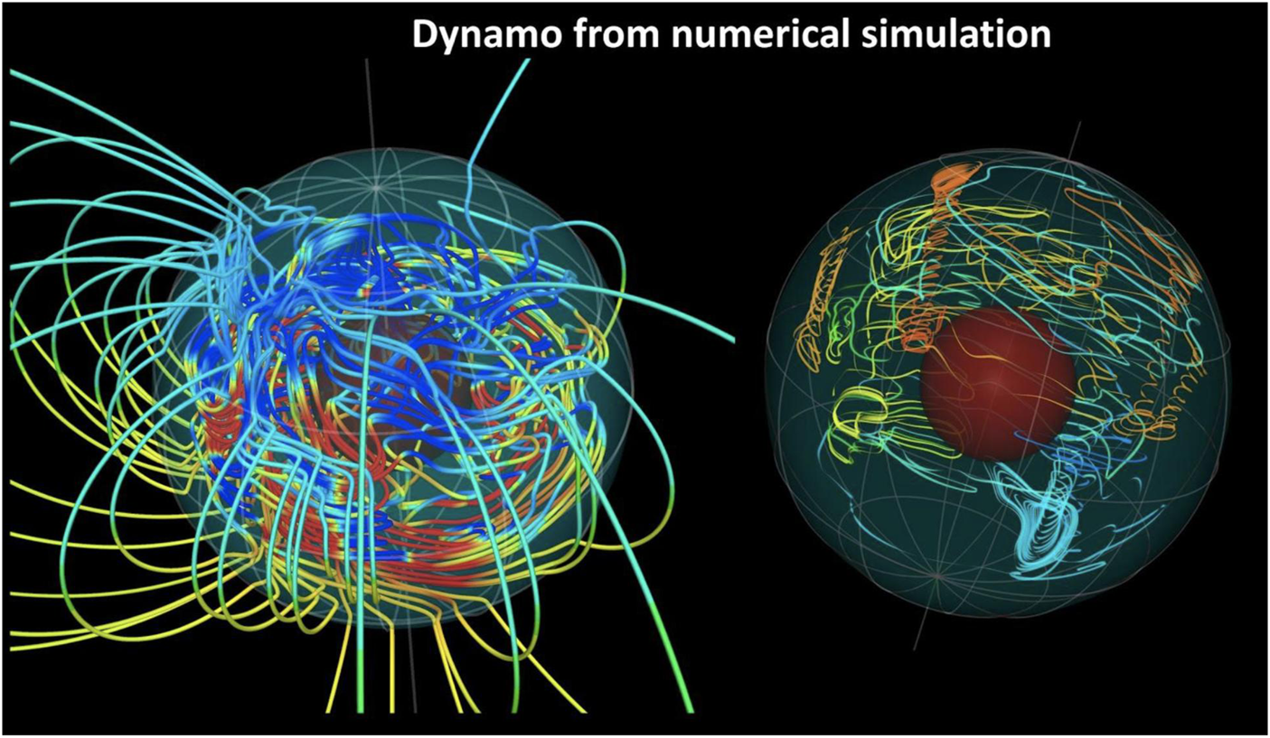
Fig. 24. Simulated planetary dynamo in a fluid outer core (between the transparent green surface at the top and the opaque red surface near the centre). The helical chaotic convective flow (on the right) generates and maintains a very complicated magnetic field (on the left) spreading out from the core to the exterior of the planet (Kuang et al., Reference Kuang, Shimizu, Airapetian, Genova, Mazarico and Goosens2019).
The working of the dynamo theory is very simple, but the resulting planetary fields can be very complex, as observed from our own Solar System: Earth has a strong (slightly tilted and dipole dominant) magnetic field over its accessible history (e.g. Biggin et al., Reference Biggin, Piispa, Pesonen, Holme, Paterson, Veikkolainen and Tauxe2015); Mercury has a very weak (off-centred dipole) field at present (Anderson et al., Reference Anderson, Johnson, Korth, Winslow, Borovsky, Purucker, Slavin, Solomon, Zuber and McNutt2012); Mars and Venus are currently non-magnetic. However, Mars had a strong magnetic field in its early history, as shown from the strongly magnetized ancient surface in the southern hemisphere detected by NASA Mars Global Surveyor (MGS) mission (Mitchell et al., Reference Mitchell, Lillis, Lin, Connerney and Acuña2007). But no similar conclusion could be made to Venus simply because of its young and hot surface. These observations suggest that a planetary magnetic field could change significantly over geological timescales, and its life-span can even be much shorter than that of the planet.
Substantial progress has been made in our understanding of the generation and the evolution of the planetary magnetic fields with large-scale numerical dynamo simulations over the past two decades (e.g. Stanley and Glatzmaier, Reference Stanley and Glatzmaier2010; Roberts and King, Reference Roberts and King2013). However, there are many fundamental questions to be answered, such as the amount of heat transport across the core-mantle boundary (e.g. Karato, Reference Karato2011; Stamenković et al., Reference Stamenković, Breuer and Spohn2011; Tackley et al., Reference Tackley, Ammann, Brodholt, Dobson and Valencia2013), and on the thermo-chemical properties of the metallic cores (e.g. Valencia et al., Reference Valencia, O'Connell and Sasselov2006; Stamenković et al., Reference Stamenković, Breuer and Spohn2011, Reference Stamenković, Noack, Breuer and Spohn2012). Their impacts on the magnetic-field generation can be far more complex than what we have understood at present time. For example, recent results of Kuang et al. (Reference Kuang, Shimizu, Airapetian, Genova, Mazarico and Goosens2019) indicate that the generation of planetary magnetic fields can be significantly weakened or even terminated if the inner core grows to beyond 50% of the outer core's radius, even though the inner core growth is vital for producing the necessary buoyancy force to drive the core dynamo. Moreover, simulations suggest that our planet could lose its magnetic field, and thus the planetary magnetospheric protection from SW effects including solar wind and energetic particles, in as short as 700 Myr with the current growth rate of the inner core (Tarduno et al., Reference Tarduno, Blackman and Mamajek2015; Bono et al., Reference Bono, Tarduno, Nimmo and Cottrell2019). Obviously, the age and thus the growth rate of the inner core depends on the geochemical properties in the Earth's core, e.g. smaller thermal conductivities can result in lower inner core growth rates (Labrosse, Reference Labrosse2015; Hirose et al., Reference Hirose, Morard, Sinmyo, Umemoto, Huernlund, Heffrich and Labrosse2017). However, these may not necessarily lead to longer geodynamo life: slower inner core growth rates imply lower amount of energy available for the geodynamo which, in turn, implies smaller inner core radii necessary to maintain the geodynamo. These results have far reaching implications for habitability of Earth-like planets around active stars including M dwarfs and imply that the planet's age should be an important habitability factor.
More observational, experimental and theoretical studies are needed for understanding the generation and evolution of the planetary magnetic fields, and for addressing the fundamental science questions directly relevant to habitable worlds, such as potential causes of destabilizing the field (e.g. magnetic polarity reversals), impacts of planetary interior structures (e.g. geometry and boundary changes) and their chemical composition (metallicity) and star–planet–moon interactions (e.g. tidal forcing on planetary fluid systems) on the planetary magnetic fields.
The magnetized planets in our Solar System provide valuable diverse dynamic systems for us to research, test and validate scientific hypothesis and models, and thus provide pathways to extrapolate results to the diversity of magnetized exoplanets. Their magnetospheres can be detected through the radio signatures introduced by the effects of the interactions between close-in exoplanets with astrospheres of their host stars. A unique Jupiter–Io interacting system, in which Io orbits within the Jupiter's magnetosphere and produces the UV-bright aurora (Mura et al., Reference Mura, Adriani, Connerney, Bolton, Altieri, Bagenal, Bonfond, Dinelli, Gérard, Greathouse, Grodent, Levin, Mauk, Moriconi, Saur, Waite, Amoroso, Cicchetti, Fabiano, Filacchione, Grassi, Migliorini, Noschese, Olivieri, Piccioni, Plainaki, Sindoni, Sordini, Tosi and Turrini2018), can serve as a good example of the planet–moon system that possibly could be detected in the closest exoplanets including TRAPPIST-1 and Proxima Centauri systems using upcoming Low Frequency Array (LOFAR) radio observations (Turnpenney et al., Reference Turnpenney, Nichols, Wynn and Burleigh2018).
Observational methods and strategies for the detection of habitable planets
The observational picture for the detection of potentially habitable Earth-sized exoplanets is bright due to continued improvements in the methods that have been used in the past 22 years after the initial discoveries of exoplanets around solar-type stars by Mayor and Queloz (Reference Mayor and Queloz1995) and Marcy and Butler (Reference Marcy and Butler1996). These researchers used the precision radial velocity method, which measures the very small Doppler shift in the velocity of the host star along the line of site to the observer, caused by the motion of the host star about the centre of mass of the two objects. In this section we focus on the strengths and limitations of each method, particularly their observational biases.
The incredible progress made in the last two decades has relied strongly on utilizing results from multiple techniques and combining them so that important physical attributes of an exoplanet can be determined, including its orbital parameters, size, effective temperature or insolation, and where enough information is available, its bulk density. Once the density is known then it is possible to determine, within appropriate observational and theoretical constraints, whether or not a given detected exoplanet is, for example, a rocky super-Earth with a thin atmosphere and the potential for a magnetic field that protects its atmosphere, or a mini-Neptune with a thick hydrogen atmosphere. Historically, most exoplanets were discovered using the radial velocity method until the photometric precision of the transit method improved to the point that it was sufficient to detect exoplanets. Both of these methods have a bias towards more massive or larger exoplanets that are relatively close to the host stars. The reason for the bias towards close-in planets for radial velocity is the relatively larger and easier to measure amplitude of the Doppler shift for a given planet mass and observational precision. The bias towards close-in planets for transit observations is related to the probability of the orbital plane of the exoplanets being close to edge-on so that the transit can be viewed along the line of sight to the observer. The likelihood of successfully observing a transit is proportional to the ratio of the diameter of the host star to the semi-major axis of the orbit of the planet. Secondly, it is also dependent on the area of the exoplanet itself compared to that of the host star, which determines the size of the signal, while the instrumental photometric precision determines the noise level.
The radial velocity method is discussed in more detail in the section ‘Radial velocity method’ and the transit method in the section ‘The transit method and transit spectroscopy’. Both methods also favour geometries that are either edge-on (transits) or within a range of angles with greatest sensitivity to mostly edge-on geometries, but limited to measuring the mass times the sine of the inclination angle (precision radial velocity).
In recent years, the gravitational lensing method has been employed to search for exoplanets beyond the snow line. This requires larger separations between the host star and planet than is accessible with the first two, on the order of several AU from the host star, typically around 4 AU or greater around a G-type star. Thus, it fills in an important observational gap. Much more will be known about these exoplanets in the future when the WFIRST mission (Spergel et al., Reference Spergel, Geherls, Baltay, Bennett, Breckinridge, Donahue, Dressler, Gaudi, Greene, Guyon, Hirata, Kalirai, Kasdin, Macintosh, Moos, Perlmutter, Postman, Rauscher, Rhodes, Wang, Weinberg, Benford, Hudson, Jeong, Mellier, Traub, Yamada, Capak, Colbert, Masters, Penny, Savransky, Stern, Zimmerman, Barry, Bartusek, Carpenter, Cheng, Content, Dekens, Demers, Grady, Jackson, Kuan, Kruk, Melton, Nemati, Parvin, Poberezhskiy, Peddie, Ruffa, Wallace, Whipple, Wollack and Zhao2015) completes its gravitational lensing observations in the 2020s. The gravitational lensing method also allows searches for exoplanets that are not bound the host star, the so-called ‘free floating’ exoplanets. These may be exoplanets that have been ejected from protoplanetary discs during the planet formation epoch, or at other stages of planetary system evolution. However, because the focus of this review is on exoplanets in the HZs of their host stars, we only mention it briefly for completeness.
The section ‘Direct imaging of rocky exoplanets’ discusses the fundamentals of direct imaging techniques, which are further developed in the sections ‘Visible wavelength direct imaging’ and ‘Infrared direct imaging’ discussing direct imaging methods in the visible and infrared, respectively. Direct imaging methods hold the most promise for the future, because they allow for all geometries, from face-on to edge-on, and with them, spectroscopic methods are employed that allow for detection of biosignature gases for exoplanets within the HZs of the host stars. A possible future ground-based observatory for the detection of exoplanets around nearby host stars is discussed in the section ‘Extremely large telescopes (ELTs) beyond the 30 m class telescopes’.
Radial velocity method
The radial velocity method was used to discover the first exoplanets as noted in the Introduction to this section. It is beyond the scope of this paper to discuss this technique in great detail. The paper by Lovis and Fischer (Reference Lovis, Fischer and Seager2010) provides a good introduction and overview. Here we provide a brief history and a discussion of the essential physics of the method. The radial velocity method has been extremely successful with >775 confirmed exoplanets as of November 2018 (http://exoplanet.eu/catalog).
The quantity measured by the radial velocity method is the semi-amplitude, K 1, which can be written in terms of quantities scaled to a Jupiter mass, the star's mass scaled to the Sun's mass, and the orbital period in years (adapted from equation (14) of Lovis and Fischer, Reference Lovis, Fischer and Seager2010), K 1 ~ (28.4/(1 − e 2)1/2)(m p/M Jup)sin(i)(M */M Sun)2/3(P/1 year)1/3 m s−1, where m p is the mass of the exoplanet, M Jup is Jupiter's mass, M * is the stellar mass, M Sun is the mass of the Sun and e is the eccentricity. If K 1 is observed over one or more complete orbital periods it is possible to determine m p sin i, the eccentricity, e and the period, P. It is also necessary to independently estimate the stellar mass, M *, which can be done by a variety of methods, in order to determine m p sin i.
A Jupiter mass planet at 1 AU has a semi-amplitude of 28.4 m s−1, whereas an Earth mass planet at 1 AU has a semi-amplitude of only 0.09 m s−1. A super-Earth of five Earth masses would have a semi-amplitude of 0.45 m s−1 at 1 AU, and 1.4 m s−1 at 0.1 AU. Thus, for a given RMS semi-amplitude precision and stellar spectral type, radial velocity detections are limited to a region of exoplanetary masses and periods that provide signals roughly of this magnitude. Repeated observations can improve the sensitivity somewhat below this naïve limit, particularly for shorter period exoplanets, where folding the radial velocity time series into a single-phase curve and averaging is possible.
The major limitation of the radial velocity technique for an exoplanet observed with this method is that only the minimum mass is measured, i.e. m p sin i, so a measurement of the inclination angle is necessary to determine the true mass. This can be done through astrometric means in which the orbit of the host star around the centre of mass of the system is measured. This can also be accomplished through direct detection methods, if the angular separation between star and the exoplanet is larger than the IWA of the coronagraph or nulling interferometer, and sufficient star–planet contrast is achieved. For statistical studies, however, this limitation may not matter as much, since the majority of observed inclination angles for randomly distributed inclinations will be between 45° and 135°. Other method to measure inclination angles relies on the observations of dust belts (Anglada-Escudé et al., Reference Anglada-Escudé, Amado, Barnes, Berdiñas, Butler, Coleman, de La Cueva, Dreizler, Endl, Giesers, Jeffers, Jenkins, Jones, Kiraga, Kürster, López-González, Marvin, Morales, Morin, Nelson, Ortiz, Ofir, Paardekooper, Reiners, Rodríguez, Rodríguez-López, Sarmiento, Strachan, Tsapras, Tuomi and Zechmeister2016).
Over the past several years, improvements to the precision of such measurements have been a major focus of the radial velocity community with the goal of achieving a precision of ~ 0.1 m s−1, sufficient to detect Earth-mass exoplanets. Besides improving the measurement precision to measure smaller exoplanet masse the community is also extending this technique to the near-infrared in order to increase the sample to include more low-mass cool stars.
Currently there are many spectrometers around the world that are being used for such exoplanet searches; essentially all are echelle spectrometers with very high resolution, of the order of R ~ 80 000 to 100 000. Unfortunately, it is beyond the scope of this paper to discuss these in detail. Listings of current and planned spectrographs can be obtained from the CARMENES website (http://carmenes.caha.es/ext/spectrographs/index.html), and also from the web page http://pendientedemigracion.ucm.es/info/Astrof/invest/actividad/echelle.html#spectrographs. An excellent reference discussing progress and challenges in the radial velocity technique is in the whitepaper from the Exoplanet Program Analysis Group (EXOPAG), Science Analysis Group (SAG), SAG-8, see Plavchan et al. (Reference Plavchan, Latham, Gaudi, Crepp, Dumusque, Furesz, Vanderburg, Blake, Fischer, Prato, White, Makarov, Marcy, Stapelfeldt, Haywood, Collier-Cameron, Quirrenbach, Mahadevan, Anglada and Muirhead2015).
CARMENES, short for Calar Alto high-Resolution search for M dwarfs with Exo-earths with Near-infrared and optical Échelle Spectrographs, is an important instrument as it is one of the first to operate in the near-infrared at the Y, J and H bands, from 950 to 1700 nm, with a resolution of about 85 000 and is in operation at the Calar Alto Observatory in Spain on the 3.5 m telescope. This instrument also has a visible wavelength channel, with a resolution of about 80 000, and is designed for a precision of ≤1 m s−1. It is optimized for searches around nearby late M-dwarf stars, thus opening up discovery space around this important class of low-mass stars (see Quirrenbach et al., Reference Quirrenbach, Amado, Caballero, Mandel, Mundt, Reiners, Ribas, Sánchez Carrasco, Seifert, Azzaro and Galadí2014 for a more detailed description of this instrument and its performance).
Another instrument that is currently under development is the Extreme Precision Doppler Spectrometer (EPDS), led by Dr Suvrath Mahadevan at Penn State University. This instrument is being funded through NASA in a joint programme with the NSF to be installed on the 3.5 m Wisconsin-Indiana-Yale-NOAO (WIYN) telescope at the Kitt Peak Observatory. This instrument has a minimum precision of 0.5 m s−1 with the ultimate goal of reaching ≤0.1 m s−1 precision, sufficient to detect Earth-mass planets around nearby stars. Note that even if such an instrumental precision is achieved, stellar effects from convection and granulation, for example, can obscure the signal from the motion of the star about the centre of mass of the system, since these effects can be of comparable size. This instrument will also be able to provide the radial velocity measurements needed for mass and orbital determination for the large number of exoplanets expected to be discovered by the TESS satellite, which was launched in 2018.
The transit method and transit spectroscopy
The transit method has been the most successful method of all of those employed so far, principally due to the incredible success of the Kepler mission. As of this writing there are over 3000 confirmed exoplanets detected with this method. In principal, the transit method is very simple: a planet passes in front of the host star viewed along the line of site to the observer, and a small dimming of the brightness of the host star can be observed. This is called the primary transit. When the exoplanet passes behind the host star, then a secondary transit occurs, which usually called the eclipse or occultation. There are many good references discussing the transit method and transit spectroscopy. An overview is given in the review paper by Winn (Reference Winn and Seager2010).
Fundamentally, the observational problem is that the amount of dimming of the host star is very small, as can be seen from a simplified formula for the transit depth, assuming R p is the radius of the planet, and R * is the stellar radius, then the transit depth δtra is δtra ≈ (R p/R *)2, where the night side emission from the exoplanet is assumed to be negligible (simplified from equation (22) of Winn (Reference Winn and Seager2010)).
For a Jupiter-sized planet around a star like the Sun, the transit depth is ~10−2, whereas the transit depth for an Earth-radius planet is ~10−4. This means the photometry should be substantially better than 100 parts per million (ppm), at least during each measurement. Systematic drifts in the photometry can be overcome by careful fitting, and repeated observations of a transit can be overlapped in a phase curve, increasing the signal-to-noise for a given detection as is done for radial velocity observations. A similar approximate formula for the depth of the secondary eclipse is, e.g. Winn (Reference Winn and Seager2010), equation (23): δecl ≈ (R p/R *)2I p(t ecl)/I *, where δecl is the eclipse depth, and I p(t ecl) is the emission or scattered light from the planet's dayside just before the planet begins its ingress behind the star and I * is the stellar intensity.
The probability of a transit varies, largely depending orbital distance of the planet to the star. In the case when the planet is much smaller than the star, and the orbit is circular, a simple formula can be derived that helps one to understand how many stars are needed to be observed in a transit survey like Kepler to achieve the desired number of detections for stars of any given spectral class and exoplanets in various size regimes, as in equation (11) in Winn (Reference Winn and Seager2010). In this equation, the symbols p tra and p ecl are the probabilities of a transit or eclipse respectively, a is the semi-major axis, p tra = p ecl ≈ 0.005(R */R Sun)(a/1 AU)−1, giving a probability of transit of 0.5% or 1/200 for an exoplanet at 1 AU for a star of the same radius as the Sun.
The transit probability is only 1/20 or 5% for an exoplanet at 0.1 AU. This equation makes it clear that an observer needs to have a large sample of stars in order to obtain a statistically meaningful number of detections of exoplanets with this method. For Kepler, in order to determine the probability of a solar-type star to have an Earth-sized exoplanet in the HZ required a sample of roughly 100 000 stars. If the entire sample consisted only of G-type stars like the Sun, then there would be 500 such detections. However, G-type stars are less than 10% of all stars in the Galaxy, giving a sample size of roughly 50 stars, if the survey lasted sufficiently long (on the order of 3–5 years) in order to make all possible detections. Also note that there is also a distribution in eccentricities that we have neglected.
Thus, sample size is one issue for transiting planet observations. Another issue is that the detection system noise should be low enough to be close to the photometric limits. A third limitation is that transits last for a few hours at most. For the case of relatively low signal to noise, the characteristic timescale of a transit, T C, adapted from equation (19) of Winn (Reference Winn and Seager2010), is T C = R *P/(πa) ≈ 13 h(P/1 year)1/3(ρ*/ρSun)−1/3, where ρ* and ρSun is the mean density of the star and the Sun, respectively. From this equation, for a star of the same density as the Sun and a planet with a 1 year orbital period, the characteristic timescale is only a few hours. This limits the observations to have a characteristic cadence, hence integration time per measurement, which much be significantly less than T C or important details in the transit light curves would be lost.
The final tool in the transit method toolkit is transit spectroscopy. As a planet with an extended atmosphere transits a star the effective radius of the planet changes as a function of wavelength due to the varying optical depth of the molecules and atoms in its atmosphere. This effect can be strong when the wavelength is at a particularly strong molecular or atomic transition. The size of the atmosphere will change by a few scale heights, H, which is given by H = k BT/(μmg), where k B, T, μm and g are Boltzmann's constant, atmospheric temperature, mean molecular weight and planet's surface gravity, respectively.
If R τ is the radius at which the optical depth is greater than unity at all wavelengths, then the fractional change in the transit depth is given by Δδ/δ ≈ 2N H(H/R τ), where N H is the number of scale heights, and the other symbols were previously defined. For an Earth-like planet (i.e. temperature, surface gravity and mean molecular weight of its atmosphere) around a star similar to the Sun, the effect is of the order of 10−2, assuming only a single scale height (see equation (36) in Winn (Reference Winn and Seager2010) for more details). The result is that the photometer must have an overall precision better than 10−6 to measure these very small changes in transit depth to characterize the atmospheres of Earth-sized planets.
The eclipse depth gives the ratio of the star to planet disc-averaged intensities as discussed previously, however, at wavelengths where the Rayleigh–Jeans approximation can be used for the Planck function, the eclipse depth as a function of wavelength reduces to δecl,them(λ) ≈ δtra(T b/T *), where T b is the brightness temperature of the planet (disc averaged), and δtra and T * are as defined previously. This equation shows that if the primary transit is measured and the stellar temperature is well-known, then it is possible to determine the brightness temperature as a function of wavelength. For the case where scattering dominates, the eclipse depth depends on the wavelength dependent geometric albedo, A λ, and the amount light scattered or reflected towards the observer, which depends on the planet radius, R p, and the semi-major axis, a, such that δecl,scat(λ) ≈ A λ(R p/a). For a Jupiter sized planet at 1 AU the eclipse depth is of the order of 10−4, and very small for an Earth-sized planet at 1 AU, of the order of one part per billion (see Winn (Reference Winn and Seager2010) equations (37)–(39) for further details).
Details of how transit and eclipse broad-band and spectroscopic observations are reduced and fitted to models of the exoplanets and their atmospheres are beyond the scope of this paper. However, there are other more recent reviews focusing on the observational literature and on potential future observations with JWST, in particular Seager and Deming (Reference Seager and Deming2010). For future observations, particularly with upcoming telescopes like JWST, we refer the reader to e.g. Beichman et al. (Reference Beichman, Benneke, Knutson, Smith, Lagage, Dressing, Latham, Lunine and Bell2008), Cowan et al. (Reference Cowan, Greene, Angerhausen, Batalha, Clampin, Colon, Crossfield, Fortney, Gaudi, Harrington, Iro, Lillie, Linsky, Lopez-Morales, Mandell and Stevenson2015) and Greene et al. (Reference Greene, Line, Montero, Fortney, Lustig-Yaeger and Luther2016).
Direct imaging of rocky exoplanets
We now turn to direct imaging of rocky exoplanets, which here means exoplanets ranging in size from that of Mars with a radius of ~0.5R E to super Earths with radii of up to ~2R E. The requirements to detect and characterize rocky exoplanets are daunting, since the light reflected by the Earth is ~10−10 that of the Sun at visible wavelengths near 0.5 and ~10−7 emitted by the Earth at 10 µm. Thus, technologies that can achieve such extremely high contrast ratios are required. Besides this high contrast requirement, direct imaging systems also require high angular resolution. For example, if the Solar System is viewed from a distance of 10 parseconds, the Earth would have an angular distance of ~0.1 arcsecond from the Sun.
The search for life in exoplanets around nearby stars is fundamentally a search for molecular constituents in the atmosphere, or biosignature gases (as discussed in the section ‘Space weather, habitability and biosignatures’), e.g. which are out of chemical equilibrium due to the presence of life. This means that at a minimum a low-resolution spectrograph is needed in addition to broadband filters that are needed for the detections. This requires a minimum size for the telescope so as to detect enough light in a narrow bandwidth of each spectral resolution element within a given exposure time.
Clearly, the orbital parameters of the exoplanets will also have to be measured, not just the semi-major axis, but also the eccentricity, inclination and line-of-nodes are necessary to characterize an exoplanet, and to determine its potential habitability. This is particularly important for direct imaging missions, in which the minimum angular resolution required depends on the maximum separation between host star and exoplanet, which occurs during maximum elongation.
These considerations also imply that if an exoplanet is not detected by an indirect method in which at least some orbital parameters can be determined as described in the previous sections of this section, a revisit strategy is necessary in order to obtain a sufficient number of observations to adequately determine the orbital parameters.
Modern visible and near-infrared (wavelengths shorter than the thermal infrared) coronagraphs create a dark hole in the region around the location of the star, and the contrast varies from the IWA with the worst performance to an outer working angle where it is best. The dark hole geometry is dependent on details of the coronagraph design. The inner work angle of most coronagraphs varies from ~2 to 4λ/D, where λ is the wavelength and D is the diameter of the telescope. Such telescopes need to have diameters of the order of 4–15 m to achieve the necessary IWA.
At thermal infrared wavelengths, defined here as those greater than about 3 µm, two main considerations lead to substantial differences in the instrumentation needed for exoplanet detection and characterization from that in visible wavelengths. First, because the wavelength is 10–20 times longer, any telescope also must be that much larger in effective diameter to obtain an equivalent IWA. Thus, in order to search a volume of space of the order of 10–30 parseconds from the Sun, a very large telescope is needed, with a diameter of roughly 20–100 m. Second, the background in the thermal infrared is extremely large compared to the expected emission from the planet and even the host star itself. For example, at 10 µm, the thermal emission for a ground-based telescope operating at ~0°C is ~109 photons per s per arcsecond2. Thus, in order to achieve the necessary sensitivity, such a telescope must be cooled to temperatures of the order of 40–50 K, like the James Webb Space Telescope. The solution to the requirement of a very large telescope is to use a dilute pupil rather than a filled one, hence an interferometer with at least two telescopes is required. For an interferometer, the angular resolution is λ/(2B), where B is the baseline, i.e. the centre-to-centre separation of the telescopes.
Visible wavelength direct imaging
In the past 20 years, great progress has been made in the development of coronagraphs for exoplanet detection. Modern coronagraphs all have heritage to the original one of Lyot (Reference Lyot1939), who developed it in order to see the coronae of the Sun. The original concept was to take the light in the image plane of the telescope and block it with a black spot or mask. The light diffracted around the spot is scattered to the edges of the pupil plane downstream, and a mask is inserted at the pupil plane to block the diffracted light. This light is further reimaged to create a new one with as much of the original starlight removed as possible, which depends on the design of both the spot or mask at the first image plane and the mask at the pupil plane. The image at the second focal plane after the pupil mask retains residual scattered light called speckles. The field of coronagraphy for exoplanet studies has exploded over the last few years, and is beyond the scope of this paper to cover in much detail. Here we capture some of the essential features and discuss the status of next generation instruments.
Currently, there are a number of systems in ground-based astronomy that are in operation, and which rely on advanced adaptive optics system to correct the wavefront coming into the coronagraph to the level necessary for the design contrast ratio. The largest contrast achievable by any ground-based coronagraph is limited in principal by the minimum number of photons that can be detected in a given fraction of the pupil (depends on the number of modes corrected in the adaptive optics or AO system) at the rate at which the AO control loop is closed, typically of the order of 1 kHz. Thus, the amount of correction to the wavefront is limited, which also means that the achievable contrast ratio is limited. Present limits for ground-based coronagraphs are contrast ratios of the order of 10−5–10−6 at a few λ/D, i.e. for the Gemini Planet Imager (GPI) (MacIntosh et al., Reference Macintosh, Graham, Ingraham, Konopacky, Marois, Perrin, Poyneer, Bauman, Barman, Burrows, Cardwell, Chilcote, De Rosa, Dillon, Doyon, Dunn, Erikson, Fitzgerald, Gavel, Goodsell, Hartung, Hibon, Kalas, Larkin, Maire, Marchis, Marley, McBride, Millar-Blanchaer, Morzinski, Norton, Oppenheimer, Palmer, Patience, Pueyo, Rantakyro, Sadakuni, Saddlemyer, Savransky, Serio, Soummer, Sivaramakrishnan, Song, Thomas, Wallace, Wiktorowicz and Wolff2014) at the Gemini South telescope, SPHERE (Langlois et al., Reference Langlois, Vigan, Moutou, Sauvage, Dohlen, Costille, Mouillet and Le Mignant2014) at the Very Large Telescope and SCExAO (Jovanovic et al., Reference Jovanovic, Martinache, Guyon, Clergeon, Singh, Kudo, Garrel, Newman, Doughty, Lozi, Males, Minowa, Hayano, Takato, Morino, Kuhn, Serabyn, Norris, Tuthill, Schworer, Stewart, Close, Huby, Perrin, Lacour, Gauchet, Vievard, Murakami, Oshiyama, Baba, Matsuo, Nishikawa, Tamura, Lai, Marchis, Duchene, Kotani and Woillez2015) at the Subaru telescope.
Techniques have been developed using deformable mirror technologies to cancel out the residual speckles and create the darkest holes possible (e.g. Oppenheimer and Hinkley, Reference Oppenheimer and Hinkley2009; Traub and Oppenheimer, Reference Traub, Oppenheimer and Seager2010; Lawson et al., Reference Lawson, Belikov, Cash, Clampin, Glassman, Guyon, Kasdin, Kern, Lyon, Mawet, Moody, Samuele, Serabyn, Sirbu and Trauger2013). The best achieved contrast in fairly recent laboratory experiments is raw contrast of 10−8, bandwidth 10%, at a central wavelength of 550 nm (Traub et al., Reference Traub, Breckinridge, Greene, Olivier Guyon, Jeremy Kasdin and Macintosh2016).
At the present time, space-based coronagraphs are being developed as part of the technology development plan from the 2010 Astrophysics Decadal Survey. The Coronagraph Instrument (CGI) is under development and it will have the best contrast ratio ever achieved in practice, expected to be of the order of 10−9 (Spergel et al., Reference Spergel, Geherls, Baltay, Bennett, Breckinridge, Donahue, Dressler, Gaudi, Greene, Guyon, Hirata, Kalirai, Kasdin, Macintosh, Moos, Perlmutter, Postman, Rauscher, Rhodes, Wang, Weinberg, Benford, Hudson, Jeong, Mellier, Traub, Yamada, Capak, Colbert, Masters, Penny, Savransky, Stern, Zimmerman, Barry, Bartusek, Carpenter, Cheng, Content, Dekens, Demers, Grady, Jackson, Kuan, Kruk, Melton, Nemati, Parvin, Poberezhskiy, Peddie, Ruffa, Wallace, Whipple, Wollack and Zhao2015). Other technologies are needed for a complete system, and as previously mentioned, a type of low-resolution spectrograph is necessary. WFIRST is developing a relatively new type of spectrograph that takes a low-resolution spectrum of every pixel in the image plane, i.e. an Integral Field Spectrograph (IFS). In order to reduce background and diffracted light (cross-talk) each pixel is imaged onto a mask at the pupil using a lenslet array, and the light from the pupil mask is sent through a prism or grism and reimaged to a focal plane in such a way that each pixel in the image plane creates a spectrum that does not overlap with the spectrum of any adjacent pixels.
With the science results achieved with the planned WFIRST CGI and the ground-based coronagraphs discussed here so far, the field is moving rapidly, and new ever improved systems are on the horizon, including instruments on the upcoming 30 m class telescopes on the ground, such as the Thirty Meter Telescope (TMT) and Giant Magellan Telescope (GMT) being developed in the USA, the European Extremely Large Telescope (E-ELT) developed by the European Southern Observatory, and the >20 m diameter Exo-Life Finder (ELF) (Kuhn et al., Reference Kuhn, Berdyugina, Capsal, Gedig, Langlois, Moretto and Thetpraphi2018), see also section ‘Extremely large telescopes (ELTs) beyond the 30 m class telescopes’. For space astronomy, the Large UltraViolet Optical InfraRed (LUVOIR) and Habitable Exoplanet (HabEx) telescopes being developed by NASA.
Infrared direct imaging
In the infrared, due to the long wavelengths, in order to obtain the necessary angular resolution required, relatively large structures are needed, and interferometry has been the preferred solution. Historically, one of the first exoplanet detection concepts was that of Bracewell (Reference Bracewell1978) who proposed a rotating two-telescope cooled space interferometer operating in the far-infrared in order to detect large cold exoplanets of the size of Neptune to Jupiter or larger. The physical principle that this concept relies on is called ‘nulling’ and it is achieved by an achromatic 180° or π radian phase-shift of the light between the two beams. The beams can be combined in the image plane or the pupil plane, and the requirement for a deep null or high contrast relies primarily on equalizing the paths from each telescope to a high precision, and on having a very small wavefront error on the beam coming from the each of the telescopes. Visualized in the plane of the sky, the result is a pattern of dark and light stripes projected on the star and its planetary system. The ‘broad-band’ dark stripe at which the path lengths are equal is centred on the star, and the maximum response to an exoplanet or other emitting material is on the first bright stripes on either side of the dark stripe. The star is much smaller than the width of the stripes, but even so, the small amount of light leakage from the star itself limits the achievable contrast. If the interferometer is rotated 180° about the line of sight to the source, a dark hole can be synthesized, with rings surrounding the dark hole where an exoplanet or other material can be detected, separated by λ/(2B).
Over the past 20 years, Bracewell's concept has been realized in both ground-based interferometers and laboratory testbeds. Two ground-based nulling interferometers have been funded by NASA. One is the Keck Interferometer with the Keck Interferometer Nuller (KIN) (Colavita et al., Reference Colavita, Serabyn, Millan-Gabet, Koresko, Akeson, Booth, Mennesson, Ragland, Appleby, Berkey, Cooper, Crawford, Creech-Eakman, Dahl, Felizardo, Garcia-Gathright, Gathright, Herstein, Hovland, Hrynevych, Ligon, Medeiros, Moore, Morrison, Paine, Palmer, Panteleeva, Smith, Swain, Smythe, Summers, Tsubota, Tyau, Vasisht, Wetherell, Wizinowich and Woillez2009; Serabyn et al., Reference Serabyn, Mennesson, Colavita, Koresko and Kuchner2012) which is no longer in operation due to funding constraints. More recently, NASA funded the Large Binocular Telescope Interferometer (LBTI) (Hinz et al., Reference Hinz, Defrere, Skemer, Bailey, Stone, Spalding, Vaz, Pinna, Puglisi, Esposito, Montoya, Downey, Leisenring, Durney, Hoffmann, Hill, Millan-Gabet, Mennesson, Danchi, Morzinski, Grenz, Skrutskie and Ertel2016). Both interferometers have key science programmes focused on obtaining measurements of the luminosity function of debris disc material (dust) in the HZs of nearby solar-type stars as well as the amount of such material in nearby stars that are likely targets for direct imaging missions.
Detailed discussions of the science of infrared interferometry for direct imaging of exoplanets and the state of the relevant technologies are beyond the scope of this paper. However, a review of the state of the art of this field was published in the chapter on ‘Infrared Direct Imaging’ (Danchi et al., Reference Danchi, Lawson Pm Absil, Akeson, Bally, Barry, Beichman, Belu, Boyce, Breckinridge, Burrows, Chen, Cole, Crisp, Danner, Deroo, Coudé du Foresto, Defrère, Ebbets, Falkowski, Gappinger, Haugabook, Hanot, Henning, Hinz, Hollis, Hunyadi, Hyland, Johnston, Kaltenegger, Kasting, Kenworthy, Ksendzov, Lane, Laughlin, Lay, Liseau, Lopez, Millan-Gabet, Martin, Mawet, Mennesson, Monnier, Murakami, Noecker, Nishikawa, Pesesen, Peters, Quillen, Ragland, Rinehart, Rottgering, Scharf, Serabyn, Tamura, Tehrani, Traub, Unwin, Wilner, Woilliez, Woolf and Zhao2009) in the 2009 Exoplanet Community Report (Lawson, Traub, and Unwin, Reference Lawson, Traub and Unwin2009). Progress in the last few years has been reviewed recently by Defrère et al. (Reference Defrère, Leger, Absil, Beichman, Biller, Danchi, Ergenzinger, Eiroa, Ertel, Fridlund, Garcia Munoz, Gillon, Glasse, Godolt, Grenfell, Kraus, Labadie, Lacour, Liseau, Martin, Mennesson, Micela, Minardi, Quanz, Rauer, Rinehart, Santos, Selsis, Surdej, Tian, Villaver, Wheatley and Wyatt2018). Briefly, laboratory testbeds developed at the end of the last decade for the Terrestrial Planet Finder-Interferometer (TPF-I) mission concept in the USA had reached contrast ratios of 1.2 × 10⁻⁵ in a 32% bandwidth at 10 µm (Peters et al., Reference Peters, Lay and Jeganathan2008), and made tests of nulling detection of Earth-sized exoplanets, including simulations of rotational modulation and chopping schemes with contrast ratios of ~10−8 for narrow bandwidths (~1%) at 10 µm (Martin et al., Reference Martin, Booth, Liewer, Raouf, Loya and Tang2012). In France, the PERSEE testbed, developed for the Darwin mission concept, achieved its goals at 9 × 10⁻⁸ in the 1.65–2.45 µm spectral band (37% bandwidth) during 100 s. This result was extended to a 7 h duration with an automatic calibration process (Le Duigou et al., Reference Le Duigou, Lozi, Cassaing, Houairi, Sorrente, Montri, Jacquinod, Reess, Pham, Lhome, Buey, Hénault, Marcotto, Girard, Mauclert, Barillot, Coudé du Foresto and Ollivier2012). These testbeds achieved the desired contrast and showed that the detection strategies worked at the level required for the mission concepts. To progress further, what remains to be done is for cryogenic testbeds to be developed with realistic signal and noise levels, appropriate for the actual astrophysical measurements.
The Large Binocular Telescope Interferometer (LBTI) Hunt for Observable Signatures of Terrestrial Planets (HOSTS) study (Danchi et al., Reference Danchi, Bailey, Bryden, Defrere, Ertel, Haniff, Hinz, Kennedy, Mennesson, Millan-Gabet, Rieke, Roberge, Serabyn, Skemer, Stapelfeldt, Weinberger, Wyatt and Vaz2016, Reference Danchi, Ertel, Defrere, Hinz, Mennesson and Kennedy2018; Hinz et al., Reference Hinz, Defrere, Skemer, Bailey, Stone, Spalding, Vaz, Pinna, Puglisi, Esposito, Montoya, Downey, Leisenring, Durney, Hoffmann, Hill, Millan-Gabet, Mennesson, Danchi, Morzinski, Grenz, Skrutskie and Ertel2016; Ertel et al., Reference Ertel, Defrere, Hinz, Mennesson, Kennedy, Danchi, Gelino, Hill, Hoffmann, Rieke, Shannon, Spalding, Stone, Vaz, Weinberger, Willems, Absil, Arbo, Bailey, Beichman, Bryden, Downey, Durney, Esposito, Gaspar, Grenz, Haniff, Leisenring, Marion, McMahon, Millan-Gabet, Montoya, Morzinski, Pinna, Power, Puglisi, Roberge, Serabyn, Skemer, Stapelfeldt, Su, Vaitheeswaran and Wyatt2018a) has recently set new limits on exozodiacal emission for solar-type stars (Ertel et al., Reference Ertel, Kennedy and Defrere2018b). With roughly half of the original sample observed (~38 stars), the detection rate is comparable for both early and solar-type stars, ranging from 71 + 11 to 20% for stars with cold dust previously detected and 8% for stars without such an excess. The upper limits on the HZ dust is 11 + 9 − 4 times the Solar System value (95% confidence limit) for all stars without cold dust, and 16 times the Solar System value for Sun-like stars not having currently detected cold dust. Upper limits for stars without an excess detected by the LBTI, the limits are approximately a factor of 2 lower.
The recent constraints on exo-zodiacal emission demonstrate the power of LBTI for vetting potential targets for future direct imaging missions such as LUVOIR (Fischer et al., Reference Fischer2018) or HabEx (Gaudi, Reference Gaudi2018). They also demonstrate the importance of completing and enlarging the study in the next few years. The WFIRST CoronaGraph Instrument (CGI) may provide additional information about the properties of the dust detected by LBTI for some of the sample, as the CGI instrument will observe scattered light from dust rather than thermal emission detected by the LBTI. The two measurements taken together allow for analyses of the physical properties of the dust grains including morphology and chemistry.
Extremely large telescopes (ELTs) beyond the 30 m class telescopes
Currently under construction are new 20+ m class extremely large telescopes being developed by teams in Europe and the United States, as mentioned in the section ‘Visible wavelength direct imaging’. Direct imaging campaigns with the sensitivity to measure exoplanet reflected light against ‘background’ light will likely depend on background- and diffraction-limited optical systems. For example, it is well-known that in this case there is a very large advantage to large-aperture optics (for telescopes of given scattered light performance). Here the integration time to achieve a given signal-to-noise ratio (S/N) scales like D −4, where D is the optical system's pupil diameter. For the exoplanet problem, where the background light is dominated by the scattered-light PSF of the optical system, the advantage of a larger aperture is even greater. In this case the exoplanet in larger optics is seen at larger angles in units of λ/D from the bright stellar background source, and smaller backgrounds.
Unfortunately, the Keck-era ground-based telescopes scale in cost like their mass which grows at least as fast as D 2. The scaling function is anchored by the Keck telescope at about $100M. This curve applies to the predicted cost of all of the planned ‘World's Largest Telescopes’ – The Giant Magellan Telescope (GMT), the Thirty Meter Telescope (TMT) and the European Extremely Large Telescope (EELT). Accounting for a fixed (in units of λ/D) telescope scattering function allows an estimate of how the achievable signal-to-noise of, for example, a 1 h Proxima-b measurement depends on wavelength pass-band and telescope aperture (Kuhn et al., Reference Kuhn, Berdyugina, Langlois, Moretto, Thiebaut, Harlingen and Halliday2014, Reference Kuhn, Berdyugina, Capsal, Gedig, Langlois, Moretto and Thetpraphi2018; Berdyugina et al., Reference Berdyugina, Kuhn, Langlois, Moretto, Krissansen-Totton, Catling, Grenfell, Santl-Temkiv, Finster, Tarter, Marchis, Hargitai and Apai2018).
One concept for an extremely large 100 m diameter class ground-based telescope is the ExoLife Finder Telescope (ELF), that is a hybrid design with multiple sub-apertures arranged on a steerable ring structure ~100 m in diameter, with a total collecting area equivalent to a single 20 m primary mirror. Each of the sub-apertures is an independent telescope, and active and adaptive optical systems can be used to co-phase all of the individual sub-apertures into a coherent image with a field of view of at least a few arcseconds in diameter. Such a ground-based system could potentially be built on a cost scale of substantially lower than conventional filled aperture telescopes since this design would not obey conventional scaling relations such as apply to the ELTs currently under construction (Kuhn et al., Reference Kuhn, Berdyugina, Capsal, Gedig, Langlois, Moretto and Thetpraphi2018).
Conclusions: future prospects and recommendations
In this paper, we described current research and promising key research areas and goals in the field of the exoplanetary SW, its roots, signatures and effects on (exo)planetary atmospheric dynamics, climates, habitability conditions and observational strategies to detect habitable planets. Here we will discuss the major directions and priorities in this emerging aspect of astrobiology – exoplanetary SW.
Current research efforts described in this paper suggests that exoplanetary SW is an emerging and vibrant field of exoplanetary science and astrobiology addressing fundamental questions at the intersection of astrophysics, heliophysics, planetary science, Earth science, chemistry and biochemistry of life.
We find that exoplanetary habitability, the critical aspect of astrobiology, is dynamic in nature, and thus should be expanded to include the impact of evolving SW from planet hosting stars. The process of evolving habitability relates to necessity of characterization of the signatures of SW from cool (G–K–M spectral type) main-sequence stars of different ages, its evolving impact on atmospheric erosion and chemistry of terrestrial exoplanets, the evolution of planetary internal dynamics, the conditions initiating prebiotic chemistry, and thus the planetary abiogenesis. The observational and theoretical characterization of these factors is a key in understanding the prerequisites for developing exobiogenic zones and atmospheric biosignatures to be observed with upcoming missions. To address these ambitious issues, a broad range of sophisticated multi-dimensional multispecies physico-chemical models that are validated for the extreme conditions in our Solar System along with laboratory experiments and new observational facilities and strategies are required. Also, the models of paleo SW and its impact on early Earth, Mars and Venus should provide better constraints for the evolving habitability in our Solar System (Airapetian, Reference Airapetian2018b). These studies will provide a framework for detection of biosignatures of life with emerging technologies in the coming decades.
The key research goals in the characterization of exoplanetary habitability and for signs of life in the next 10–20 years should include the following:
Characterization of space weather from planet hosting stars
Understanding the drivers and fluxes of ionizing radiation from F–M type stars hosting exoplanets is critical for characterization of their impact on exoplanetary atmospheres, will be an organic component of exoplanetary science over the next 10–20 years. Given the current progress in developing theoretical modelling and observational tools required for such characterization, we urge the committee to consider the following recommendations:
(1) Recognize that modelling of extended astrospheres of stars hosting planets is one of the major components for characterizing habitable exoplanets, especially impacts on atmospheric erosion, chemistry and surface radiation dosages.
(2) Promote the development of coordinated multi-wavelength multi-observatory programmes to derive critical inputs for theoretical and empirical tools using X-ray, FUV, NUV, radio observations and surface magnetic-field maps (magnetograms). The community should strongly encourage the development of new X-ray space telescope (see Wolk et al., Reference Wolk, Drake and Branduardi-Raymont2019), FUV/NUV space telescope (The Star–Planet Activity Research CubeSat (SPARCS), see Scowen et al., Reference Scowen, Shkolnik, Ardila, Berman, Beasley, Bowman, Fitzgerald, Gorjian, Jacobs, Jewell, Llama, Meadows, Nikzad, Spittler, Swain and Zellem2018; UV space probe mission, CETUS, Danchi et al., Reference Danchi, Ertel, Defrere, Hinz, Mennesson and Kennedy2018, Colorado Ultraviolet Transit Experiment (CUTE), Fleming+ 2018) missions, and radio telescope facilities (LOFAR and Very large Array (ngVLA) (Osten et al., Reference Osten, Crosley, Güdel, Kowalski, Lazio, Linsky, Murphy and White2018) to open new windows into the nature of nearby planet hosting stars. Characterization of stellar magnetic activity signatures include characterization of dynamics of magnetic starspots and their association with (super)flares using data from Kepler, TESS and the upcoming missions including CHEOPS, JWST, PLATO 2.0 and ARIEL. A comprehensive description of flaring properties (frequency, maximum energy, energy partition) is a crucial component of exoplanetary atmospheric evolution models.
(3) Perform direct, detailed characterization of stellar magnetic fields, in particular those of key exoplanet host stars, through high-resolution spectroscopy, spectropolarimetry and interferometric polarimetry using data obtained with ground-based optical and infrared facilities including the upcoming instrument SPIRou for infrared spectropolarimetry at the CFHT. Characterize the evolution of stellar magnetic structures in large samples of stars using indirect proxies, including spots and their association with flares using data from Kepler, TESS and upcoming missions including CHEOPS, JWST, PLATO 2.0 and ARIEL. Develop dynamo models of F–M stars.
(4) Refine the characterization of the ages of planet hosting stars using Li, rotation rates, CaII H&K and patterns of magnetic activity in the form of frequency distribution of stellar flares, their duration and maximum energy and maximal sizes of starspots. Thus, dedicated observations and comprehensive characterization of flares at different phases of evolution of F–M stars are required along with flare frequency.
(5) Encourage the extension of heliospheric MHD, kinetic and hybrid models to be used for reconstruction of coronal properties, XUV fluxes and stellar wind properties from G–K–M dwarfs using empirical and theoretical models that incorporate coordinated X-ray, FUV, NUV, optical, radio (with next generation Very large Array (ngVLA)) and mm emission and surface magnetic-field observations (magnetograms). This requires a multi-observatory network of coordinated observations using ground-based and space telescopes including TESS, HST, NICER and XMM-Newton.
(6) Develop MHD models for initiation and development of stellar flares and CMEs. These models can also be used to characterize the magnetic connectivity between a star and a planet. This is important for SW impact on habitability as it will determine (for instance) the trajectories of stellar energetic particles. These models should also characterize the impact of activity transmission spectra of exoplanets, which is an unexplored area.
(7) Search for stellar CMEs from active stars based on an array of X-ray, UV and radio observations as predicted by current and future multi-dimensional MHD models.
(8) Characterization of stellar ages of planet hosting stars based on a set of observables including Li, rotation rates, CaII H&K, patterns of magnetic activity. Dedicated observations of flares on G–K–M stars at different phases of evolution are required along with characterization of flare frequency.
Characterization of star–planet interactions
1. Development of multi-dimensional multi-fluid MHD, hydrodynamic and kinetic models that describe the coupling of energy flows between star and planet as well as energy transfer and dissipation in exoplanetary magnetosphere–ionosphere–thermosphere–mesosphere environments. This requires a well-coordinated interdisciplinary effort from the cross-disciplinary community including heliophysics, astrophysics, planetary and Earth science.
2. Derive thresholds of impact of astrospheric SW on factors of habitability including atmospheric escape (thermal and non-thermal escape rates) from exoplanets around F–M dwarfs.
3. Characterize chemistry changes due to: steady state and transient FUV, XUV fluxes, stellar winds, CMEs and energetic particles.
4. Search for radio and optical stellar CME signatures by performing extended long-term observations at lower frequencies (<10 MHz) with space or lunar radio missions.
5. Search for planetary outflows in spectral lines of H (hot Jupiters) and nitrogen and metals (terrestrial planets) driven by powerful stellar flares from active G–K–M dwarfs.
6. Explore when M dwarf habitable cases actually shift beyond the ice line due to severe SW, when combined with ameliorating internal heating, including radiogenic sources as well as tidal heating within compact multi-body TRAPPIST-1 analogue systems.
Characterization of exoplanetary environments
1. Understanding of mechanisms of ionosphere–thermosphere–mesosphere (MIT) system response to extreme SW on the early Earth, Mars and exoplanets. This includes the development of multi-dimensional modelling efforts of MIT system to characterization of the rates of atmospheric erosion resulting from various modes of star–planet interactions and resulting atmospheric thermodynamics and chemistry.
2. Search for signatures of nitrogen-rich atmospheres through UV and mid-IR bands using transmission and direct imaging observations, as necessary to determine how common they are in terrestrial-type exoplanets in the solar neighbourhood.
3. Detection and characterization of atmospheric signatures of hydrogen-rich (primary atmospheres) of terrestrial-type exoplanets around very young planet hosting stars.
4. Detection and characterization of N2–CO2–H2O rich atmospheres through identification of spectral atmospheric signatures of young terrestrial-type exoplanets at a pre-life phase: signatures of prebiotic chemistry.
5. Extension of 3D Global Climate modelling efforts to include diverse chemistry of exoplanetary atmospheres impacted by volcanic activity and SW factors.
6. Modelling and laboratory experiments of atmospheric biosignatures of life guided by prebiotic chemistry and observations of Earth's upper atmosphere in response to current SW. This includes theoretical and laboratory studies of the initiation of prebiotic chemistry and biochemical pathways to the building blocks of life as we know it.
7. Characterization of exoplanetary magnetic dynamos, mantle activity and the interplay between volcanic/tectonic activity and the role exomoons in the generation and maintaining exoplanetary magnetic dynamos. Magnetospheric low-frequency radio observations provide crucial information about exoplanetary magnetic field, the factor of habitability (Lazio et al., Reference Lazio, Hallinan, Airapetian, Brain, Dong, Driscoll, Griessmeier, Farrell, Kasper, Murphy, Rogers, Shkolnik, Stanley, Strugarek, Turner, Wolszczan, Zarka, Knapp, Lynch and Turner2018).
8. Instrument development in support of direct imaging exoplanetary missions to detect atmospheric biosignatures in the mid-infrared band including characterization of host stars in the FUV and X-ray bands.
Acknowledgements
The authors thank the referee, Prof. Lena Noack, for her constructive suggestions that improved this paper. V. Airapetian was supported by NASA Exobiology grant #80NSSC17K0463 and TESS Cycle 1. V. Airapetian, A. Glocer, K. Garcia-Sage, W. Kuang, W. Danchi, G. Gronoff and M. Way were partially supported by Sellers Exoplanetary Environments Collaboration (SEEC) Internal Scientist Funding Model (ISFM). The part of O. Verkhoglyadova’s work was performed at the Jet Propulsion Laboratory, California Institute of Technology, under a contract with NASA.


