2. Numerical method and simulations

All solutions were obtained by solving the Navier–Stokes equations for compressible flow (see, e.g. chapter 5, Tannehill, Anderson & Pletcher (Reference Tannehill, Anderson and Pletcher1997)). The numerical method was implemented in an in-house code developed by, and as described in, Patel (Reference Patel2018). The code implements explicit, second-order, Runge–Kutta time stepping, and sixth-order compact differences for spatial derivatives on non-uniform grids. Here, a Cartesian grid was used, with non-uniform spacing for clustering at the shear layer near inflow, and stretching in geometric progression in lateral and streamwise directions. The LES is obtained by the explicit filtering method proposed in Mathew et al. (Reference Mathew, Lechner, Foysi, Sesterhenn and Friedrich2003), which is a nearly equivalent implementation of the approximate deconvolution method (known as ADM) of Stolz & Adams (Reference Stolz and Adams1999). Aside from the several flows reported when the approximate deconvolution method was developed, many more have been reported from Air Force Research Laboratory where the present filtering approach was used (e.g. Visbal & Rizzetta Reference Visbal and Rizzetta2002; Rizzetta, Visbal & Morgan Reference Rizzetta, Visbal and Morgan2008). A similar approach, termed selective filtering has been used at École Centrale de Lyon for LES of jets (Bogey & Bailly Reference Bogey and Bailly2006). Examples from our laboratory are in Patel (Reference Patel2018) and Mathew (Reference Mathew2016).

A Cartesian coordinate system is used with the $x$-axis aligned with the streamwise direction. Velocity components are $u(x,y,z,t)$, $v$, $w$ in the $x$, $y$ and $z$ directions. Means are $U(x,y,z)$, $V$, $W$ and fluctuations are $u'(x,y,z,t)$, $v'$, $w'$. At the inflow plane, no-slip, isothermal conditions were specified at the wall. The jets were specified by setting the streamwise velocity component to have a top-hat profile with a tanh variation at the jet boundary. Cross-flow components were set to zero and pressure was set to a constant value. The density profile was then obtained from the Crocco–Busemann relation. Wherever the flow crosses a computational boundary, non-reflecting conditions, described in Poinsot & Lele (Reference Poinsot and Lele1992) and termed NSCBCs, were applied. These boundary surfaces comprise the jet portion of the inflow plane, lateral boundary planes, and the downstream outflow plane. Near the lateral and outflow boundaries, there is a sponge layer where a smoothing filter was applied to transported variables (Bogey & Bailly Reference Bogey and Bailly2002). The combination of the coarse mesh and filter causes fine scale fluctuations in the jet to disappear and ensures that there is no reverse flow at the outflow boundary. Then, standard, non-reflecting conditions are effective. The profiles at the inflow plane mentioned above are steady target values. Navier–Stokes characteristic boundary conditions applied at the inflow plane provides unsteady perturbations consistent with allowing waves from within to leave without reflection. A weighted sum of these unsteady profiles and the steady target profiles are applied as the boundary conditions on the inflow plane to prevent drift, as proposed in Bogey & Bailly (Reference Bogey and Bailly2006). It has not been necessary to add any fluctuations to the target profiles because these waves were sufficient to excite the shear layer instability.

The code has been validated extensively with tests ranging from acoustic wave propagation to LES of turbulent subsonic and supersonic (over- and under-expanded) jets (Patel Reference Patel2018; Patel & Mathew Reference Patel and Mathew2019). Here, a simulation of a single round jet serves as a further validation relevant to the twin jet study. Grid requirements were understood from extensive single jet simulations.

Rectangular domains and Cartesian grids were used. Parameters of the different simulations are listed in table 1. Case SR120 is a single jet at ${Re} = 11\,000$, which is the well known benchmark experiment of Panchapakesan & Lumley (Reference Panchapakesan and Lumley1993). In the cross-plane the grid was uniformly spaced over the cross-section of the jet up to $1.5d$, with spacing $d/12$, then stretched at 1 % up to $12.5d$, and then at 10 % until $y = \pm L_y$ or $z=\pm L_z$. In table 1, $N_d$ is the number of grid points across the diameter of the jet at the inflow plane. Grid spacing in the streamwise direction was increased from inflow itself at a uniform rate of 0.7 %. There were 20 additional grid planes at the lateral boundaries and 31 at the outflow for sponge zones. Case TR255 is the experiment of Okamoto et al. (Reference Okamoto, Yagita, Watanabe and Kuwamura1985) with spacing $S/d=5$ at ${Re}=230\,000$. In the $y$–$z$ plane, there are 25 gridpoints across each jet at inflow, uniform spacing up to $4.5d$, 1 % stretching until $10d$ and 10 % beyond to the lateral boundaries. Streamwise stretch rate was 0.6 %. Results of varying nozzle spacing were obtained at the lower ${Re}=25\,000$ of the experiments in Harima et al. (Reference Harima, Fujita and Osaka2005). For these three cases the differences are the extent of the uniform region around the individual jet, and the larger cross-section of $64d \times 64d$ ($70d \times 70d$ for TR248). Typically, each simulation was run from the beginning for 10 nominal flow-through times so that a stationary state was obtained before collecting statistics from time series over 35 or more flow-throughs. Here, a flow-through time is the scale $L_x/U_j$, though fluid particles will take longer as the flow decelerates.

Table 1.

Parameters of the LES. Case label indicates type of jet, number of points across jet diameter $N_d$ and nozzle spacing. Here, $L_z=L_y$ and $N_z=N_y$.

The single round jet at ${Re}=11\,000$ develops shear layer instabilities and subsequently breaks down into turbulence by $x/d=5$. In the turbulent region, jet half-width grows linearly with growth rate 0.094, which is close to the value of 0.096 in Panchapakesan & Lumley (Reference Panchapakesan and Lumley1993). The reciprocal of the mean centreline velocity $U_c$, scaled with its value $U_j$ at the inflow plane, grows linearly with distance as shown in figure 1(a). The slope is $1/6.06$; in the experiment too it was 1/6.06. In under-resolved LES, the $1/U_c$ curve will be slightly curved. Root mean square (r.m.s.) of fluctuations become very nearly constant when scaled with centreline velocity as shown in figure 1(b), as in the experiment.

Figure 1.

Self-preservation in mean and fluctuations of velocity in a single round jet at $Re=11\,000$ compared with the experiment of Panchapakesan & Lumley (Reference Panchapakesan and Lumley1993). (a) Reciprocal of centreline velocity: LES (——, blue); experiment (– – –, black). (b) Velocity fluctuations: LES, $u_{rms}$ (——, blue); LES, $v_{rms}$ (– – –, blue); experiment, $u_{rms}$ ($\circ$, red); experiment, $v_{rms}$ ($\square$, red).

Figure 2 shows radial profiles at several stations $8 \le x/d \le 70$ of the mean and fluctuations of the streamwise velocity component. Profiles of the mean are still developing at $8d$ and $10d$, but beyond $15d$ there is no change when scaled with local centreline velocity $U_c$ and half-width $r_{1/2}$ (figure 2a). Close quantitative agreement with the profile from the experiments of Panchapakesan & Lumley (Reference Panchapakesan and Lumley1993) has been obtained. Fluctuations also relax to a common profile on these scales. In figure 2(b) the two dashed curves are for $x/d = 8, 15$. Fluctuation levels in the LES are slightly smaller than in the experiment. Smoother curves and smaller variance would need longer sampling times, but it should be clear that scaled fluctuations also collapse. Profiles of the fluctuations of transverse component $v_{rms}$ were similar (not shown here). Figure 3(a) shows power spectral density curves from time series of the streamwise velocity component along the jet axis at $x/d=35$ and 48. A power-law region is evident and the spectra also collapse on local scales. These LES results are qualitative and quantitative indications of the adequacy of the simulations.

Figure 2.

Radial profiles of mean and fluctuations of streamwise velocity component, scaled with local centreline velocity $U_c$ and half-width $r_{1/2}$, from the single jet case SR120. (a) Profiles of streamwise component of mean velocity at $x/d = 8$, 10 and $15, 20, 25, \ldots 70$. Profiles for $15 \le x/d \le 70$ collapse to a single curve. Differences are seen for $x/d= 8, 10$. Symbols from the experiment of Panchapakesan & Lumley (Reference Panchapakesan and Lumley1993), curves from LES. (b) Radial profiles of streamwise velocity fluctuations $u_{rms}$ on planes $x/d = 8, 10$ (– – –, red), $15 \le x/d \le 65$ (——, blue); symbols from the experiment of Panchapakesan & Lumley (Reference Panchapakesan and Lumley1993).

Figure 3.

Power spectral density $E(f)$ of streamwise velocity component $u(x,0,0,t)$. Scaled with local scales $U_c$ and $r_{1/2}$ (case SR120), and $U_m$ and $y_{1/2}$ (case TR255). (a) Single jet, $x/d= 35$ (– – –, red), 48 (——, blue). (b) Twin jet.

3. Structure of turbulent, twin round jets

Large-eddy simulations at the conditions of the experiment in Okamoto et al. (Reference Okamoto, Yagita, Watanabe and Kuwamura1985) at ${Re} = 230\,000$, corresponding to mean velocity at centreline, $U_j = 47$ m s$^{-1}$, were performed. Of the two configurations they reported, the following discussion is for $S/d=5$ (case TR255 in table 1). A test simulation was performed on a coarser grid which had 10 points across each jet at inflow, resulting in a grid of size $203 \times 159 \times 159$ points. By comparing velocity profiles at several stations it was observed that, everywhere, the finer grid solution agreed more closely with experiment. This convergence with improving spatial resolution was expected because it has been observed to be a feature of the present LES model in many previous examples (Mathew et al. Reference Mathew, Lechner, Foysi, Sesterhenn and Friedrich2003; Mathew Reference Mathew2016). A significant difference (error) on the coarse grid was that the large scales were more active and the merger took place earlier, completed by $35d$, whereas in the experiment, and on the finer grid, merger is approximately $10d$ farther downstream.

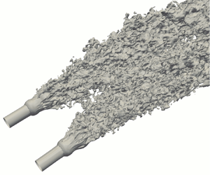
An impression of the twin jet solution can be obtained from the visualization in figure 4 where isosurfaces of velocity magnitude are shown. Laminar jets emerge from the nozzles and roll up into rings which break down into turbulence. These turbulent jets merge to form a single jet, initially with an elliptic cross-section.

Figure 4.

A twin round jet visualized with isosurfaces of velocity magnitude at an instant from case TR255.

3.1. Mean quantities

Figure 5 shows distributions of the streamwise velocity component at an instant, and the mean, together with a few streamlines. The boundary conditions permit weak flows to enter from the lateral boundaries and get entrained by the jets. Note that there is no significant bending of the jets towards each other – unlike in twin plane jets; so the initial development is rather like that of single jets. The development of jet velocity $U_n$ on the lines $y=\pm S/2$, $z=0$ through the nozzle centres, and $U_c$ along the configuration centreline ($y= z =0$), are compared with experiment in figure 6(a). The maximum velocity $U_m(x)$ at a section is the larger of $U_n(x)$ and $U_c(x)$. Initially $U_m(x)$ occurs on the nozzle axis; during merging, it moves to the $x$-axis. The velocity $U_m(x)$ from simulation is compared with experiment in figure 6(b). Okamoto et al. (Reference Okamoto, Yagita, Watanabe and Kuwamura1985) had used $U_m$ to normalize the velocity data. Here we find it to permit some, limited, scaling of the data. We will also use the distance $y_{1/2}$ from the configuration axis to the point where the velocity $U(x, y; z=0)$ falls to $U_m(x)/2$ as a local reference length, analogous to the half-width of single jets.

Figure 5.

Streamwise component of velocity on plane $z=0$ from LES of case TR255. (a) Streamwise velocity $u(x,y,0,t)$ (m s$^{-1}$). (b) Mean streamwise velocity $U(x,y,0)$ (m s$^{-1}$) and streamlines.

Figure 6.

Development of mean streamwise velocity for case TR255. (a) Decay compared with measurement along nozzle axis: $U_n$, LES (——, blue); $U_n$, experiment (– – –, red); $U_c$, LES (– $\bullet$ –, blue); $U_c$, experiment ($\circ$, red). (b) Maximum at any cross-section, initially within individual jets and along $x$-axis after jets merge: $U_n$, LES (——, blue); $U_c$, experiment ($\bullet$, red).

From time series $u(x,0,0,t)$ at stations along the $x$-axis, the development of the energy spectrum normalized using $U_m$ and $y_{1/2}$ is shown in figure 3(b). Beyond $x/d=28$, the spectra do collapse even though merger is not yet complete and $U_m$ is not yet on the configuration centreline (see figure 8a below). It is perhaps not surprising then that fluctuation levels over a central part of the merged jet also scale with $U_m$ (see figure 9 and discussion below).

Jet width growths are shown in figure 7, by taking jet boundary to be where $U = 0.1U_m$, as reported in the experiment, instead of the more common half-width. The merging jets occupy an elliptical region, with the major axis in the $x$–$y$ plane, which then relaxes to a circular region with a slight over-shoot. Growth of the half-width of single round jets has been included, but it is worth remembering that measurements near the outer edges of shear flows are not as reliable due to flow reversals. The initial spreading in the $x$–$y$ plane is slightly smaller than that of single jets in both LES and experiment – differences are smaller downstream of merger. Axis switching appears as a mild reversal in growth. In the $x$–$z$ plane of the nozzle axis of either jet ($y=S/2$), growth rates in LES and experiment are closer to that of single jets. Due to possible differences in inflow conditions, evident in velocity $U_n(x)$ also (figure 6a), the widths in figure 7(b) are different for $x/d < 10$, but the slopes are very nearly the same downstream. We shall return to this below while discussing pressure distributions.

Figure 7.

Jet spreading in two planes. Jet boundary is located where mean velocity $U$ is 10 % of the maximum over cross-section ($x$, constant): experiment ($\bullet$, red); LES (–$\blacksquare$–, blue); single jet (– – –). (a) On $z=0$ and (b) on $y=S/2$.

Profiles of mean velocity at several downstream locations are shown in figure 8(a). Before merging, the maximum velocity is still within individual jets ($x/d=20$, 28), but the velocity in the region between the jets is increasing (is within 90 % of $U_m$ at $x =35d$). Generally, there is very close quantitative agreement with experiment over most of the jet. Small differences are evident near the outer boundary for $x > 28d$.

Figure 8.

Radial profiles of mean streamwise velocity and pressure coefficient for case TR255: blue curves, LES; symbols (experiment, Okamoto et al. Reference Okamoto, Yagita, Watanabe and Kuwamura1985) at $x/d = 10$ ($\circ$, red), 20 ($\blacksquare$, red), 28 ($\blacktriangle$, red), 48 ($\bullet$, red). (a)  Streamwise velocity. (b)  Pressure coefficient.

Figure 8(b) is a comparison of radial pressure profiles between LES and experiment. Close quantitative agreement has been obtained. The pressure coefficient $C_p = (p-p_{\infty })/\frac {1}{2}\rho _{\infty }U_j^2$, where $p_{\infty }$ and $\rho _{\infty }$ are the pressure and density in the far field. The pressure is generally considered to be uniform in free shear flows. But, there is a small gradient across the shear layer which would balance fluctuations of the radial component of velocity (Tennekes & Lumley Reference Tennekes and Lumley1972, chapter 4). The approximation is acceptable since the maximum difference in pressure is small: it is only approximately 0.1 % of the inflow plane dynamic pressure in the single jet region (see curve for $x/d=48$ in figure 8b). In the twin jet configuration, we observe the pressure difference to be significantly larger before the jets merge – approximately 3 %–4 % of dynamic pressure at $x/d=10$. In turn, this radial gradient would be consistent with a slightly smaller radial spreading than in a uniform pressure field. In figure 7(a), the spreading of the twin jet in the $x$–$y$ plane is slightly less than that of single jets initially but appears to be at nearly the same rate beyond $x/d=40$. As the merged elliptic form relaxes to a round jet, and the radial pressure gradient diminishes, the difference in spread rate should also disappear. The difference between twin jet and single jet is noticeably less in the $x$–$z$ plane; consistently, the maximum difference in $C_p$ across the jet in $x$–$z$ planes was found to remain less than $-0.003$ % of dynamic pressure (not shown).

3.2. Turbulence intensities and Reynolds shear stress

Okamoto et al. (Reference Okamoto, Yagita, Watanabe and Kuwamura1985) had not provided turbulent fluctuation measurements. In single jets, turbulence intensity scales with the mean centreline velocity, and radial extent on the half-width. In twin jets, we may expect the same scaling to hold good far downstream. In the developing region, by definition, we do not expect any such scaling. However, it turns out that fluctuations do scale with the maximum velocity $U_m$ even where the merged jet is developing into the round jet. Figure 9 shows profiles of fluctuations along two lines ($y$; $z=0$) and ($y=0$; $z$) at several $y$–$z$ planes. Quantities are normalized with $U_m$ and length $y_{1/2}$.

Figure 9.

(a–f) Fluctuation profiles and (g,h) Reynolds shear stress profiles. All are normalized with maximum of local mean streamwise velocity $U_m$ and distance $y_{1/2}$. Here, $x/d = 8$ ($\circ$, red), 10 ($\bullet$, red), 15 ($\blacksquare$, red), 20 (——, blue), 25 (– – –, blue), 30 (– $\bullet$ –, blue), 35 (——, green), 40 (– – –, green), 45 (– $\bullet$ –, green), 50 (–$\circ$–).

Consider first figure 9(a,c,e,g). Curves with red symbols for $x/d=8, 10, 15$ show the development of fluctuations. The continuous ones are for $20 \le x/d \le 50$. Generally, for $x/d > 20$, all the curves collapse over $y < y_{1/2}$ which is the width of a core region wherein fluctuation levels are nearly uniform and scale with $U_m$. In single round jets also, fluctuation levels are nearly uniform within the half-radius (Panchapakesan & Lumley (Reference Panchapakesan and Lumley1993); figure 2b). The length $y_{1/2}$ is a scale for jet width before merger ($x/d < 20$) and thereafter for the extent of the turbulent core, but not the jet width. Of course, since the fluctuation levels in the core are nearly uniform, these curves suggest a common profile on a shifted local coordinate $(y-y_{1/2})/\delta$, where $\delta$ would be the width over which the velocity $U(y)$ drops from $U_m$ to zero. Figure 9(b,d,f,h) contains profiles along the $z$-axis. Since the turbulence level is larger near the centre of the individual jets even as they merge, fluctuations levels in the $y=0$ plane continue to develop for quite some distance downstream. In figure 9(b), $u_{rms}/U_m$ approaches its downstream value by $x/d \approx 30$ near the axis but the extent of this region continues to increase. The development of transverse fluctuation to the far downstream levels (amplitude and extent of region) is not very different. Figure 9(g) shows the development of Reynolds shear stress component $\langle u'v'\rangle$ along $y, z=0$. The distribution for $x/d \le 40$ is consistent with an outer and inner shear layer of the individual jets. It is only by $x/d = 45$ that traces of the inner shear layer has ended. Figure 9(h) shows the development of component $\langle u'w'\rangle$ along $z, y=0$; these profiles have the same shape but other scales for velocity and extent are needed.

All the comparisons with the experiment of Okamoto et al. (Reference Okamoto, Yagita, Watanabe and Kuwamura1985) serve to confirm that the LES provides a very accurate description of large scale features of twin round jets at the large Reynolds number, 230 000, of relevance to practical applications. Okamoto et al. (Reference Okamoto, Yagita, Watanabe and Kuwamura1985) had used the maximum velocity $U_m$ at streamwise stations to normalize the data. We observe from the simulation data that $U_m$ is a velocity scale for turbulent fluctuations. In the following section, we examine the effects of nozzle spacing $S$.

4. Nozzle spacing effects

Nozzle spacing effects were studied by performing LES at the conditions in Harima et al. (Reference Harima, Fujita and Osaka2005) for three nozzle spacings $S/d=2, 4$ and 8 at ${Re} = 25\,000$. Turbulence scalings are well-established in round jets by ${Re} \sim O(10^4)$ itself; e.g. the benchmark by Panchapakesan & Lumley (Reference Panchapakesan and Lumley1993) is at 11 000. Simulation domain and grid sizes are listed in table 1. Grids are similar in all cases, with 24 points across the jet, uniform spacing to $1.5d$ around each jet and then mild stretching outward ending with a coarsely spaced buffer zone.

The solutions are shown in figure 10 as contours of the streamwise velocity at an instant on the plane $z=0$. Not surprisingly, flow fields of all cases are similar to the solution for $S/d= 5$ that was discussed in § 3 above. Each jet grows by turbulent entrainment with little effect on the other until both become part of an initially elliptical region. Merging occurs farther downstream as $S/d$ is increased. Mean fields revealed that there is a mild bending towards each other when the spacing is large ($S/d=8$); the bending is quite small even at $S/d=5$ (see figure 5b above). When the nozzle spacing is quite small, the jets begin to interact before breakdown to turbulence is completed: figure 10(a) for $S/d=2$ shows merger to begin at the vortex ring stage itself; when the spacing is larger, say, $S/d=4$ (figure 10b), individual jets have broken down before merger begins. Thus, the initial development for $S/d=2$ is different from the others. Large spacing brings in differences to later development: for $S/d=8$, there is a mild bending of the two jets towards each other, and the larger aspect ratio of the elliptic region on merger results in a slower relaxation to a single round jet.

Figure 10.

Streamwise component of velocity at an instant on plane $z=0$ from LES at Re = 25 000. (a) $S/d = 2$, (b) $S/d = 4$, (c) $S/d = 8$.

For turbulent single round jets that emerge from a nozzle of diameter $d$ with a near uniform velocity $U_j$, these input parameters serve as scales for the configuration. Local, intrinsic scales are the centreline velocity $U_c$ and half-width $r_{1/2}$. Assuming self-preservation, we can derive power law relations for these local scales in terms of the input parameters $U_j$ and $d$. Experiments show these relations to hold from a short distance downstream of the breakdown to turbulence. For twin round jets, the input parameters are $U_j$, $d$ and $S$. It is reasonable to expect the far downstream structure to be similar to single jets. However, we find that the near field also has intrinsic scales on which the development collapses into a single curve for the range of nozzle spacings simulated.

Curves in figure 11(a) are of the development of mean streamwise velocity along the configuration centreline $U(x,y=0, z=0)$ from the four twin-jet simulations and the two experiments. There is an initial rise as jets interact and then a decay in the combined jet. The growth and decay are sharper for closely spaced nozzles; the peak value is smaller and occurs increasingly farther downstream as nozzle spacing increases because centreline velocities of individual jets will have decayed more before merging. The data from the simulations are very close to those from the experiments for $S/d=4$ (Harima et al. Reference Harima, Fujita and Osaka2001) and $S/d=5$ (Okamoto et al. Reference Okamoto, Yagita, Watanabe and Kuwamura1985), but clearly different for the other two cases. We suppose the differences to be due to differences in conditions at the nozzle exit. In turn there are effects on the initial development: as pointed out while discussing figure 10, the closely spaced jets merge before breakdown to turbulence is completed, while at the largest spacing there is a slight bending towards each other. So, no attempt was made to find an inflow condition that would give closer agreement with Harima et al. (Reference Harima, Fujita and Osaka2001) for all spacings. In spite of such differences, it turns out that data from both experiment and simulation support a new intrinsic scaling.

Figure 11.

Development of streamwise velocity along configuration axis $y=0, z=0$ for $2 \le S/d \le 8$. (a)  Scaled with input parameters; $U_c(x)$. (b) Scaled with peak velocity $U_0$ and distance to peak $L_0$; $U_c(x)$ scaled with $U_0$ and $L_0$. For LES: $S/d=2$ (——, blue), 4 (– – –, red), 5 (– $\bullet$ –, green), 8 (– $\bullet$ $\bullet$ –). For experiment (Harima et al. Reference Harima, Fujita and Osaka2001): $S/d=2$ ($\bullet$, blue), 4 ($\blacktriangle$, red), 8 ($\blacksquare$). For experiment (Okamoto et al. Reference Okamoto, Yagita, Watanabe and Kuwamura1985): $S/d=5$ ($\blacktriangledown$, green).

Let $U_0$, the maximum of $U_c$, be a velocity scale, and the distance from the wall $L_0$ where this maximum is reached be a length scale. Remarkably, when the development of centreline velocity is rescaled, $U_c/U_0$ is seen to be a function of $x/L_0$, independent of $S/d$ (figure 11b). So, these are intrinsic length scales of the similar, initial development of twin jets. It remains to connect these intrinsic scales to the input parameters. Figure 12(a) shows the dependence of $U_0$ scaled with jet inflow velocity $U_j$ on $S/d$. Over this range, for the LES data, $U_0/U_j = 1/(1.02S/d + 0.44)$. The length scale also has an essentially linear dependence: $L_0/d = 5.58S/d - 1.16$ (figure 12b). For the experiments of Harima et al. (Reference Harima, Fujita and Osaka2001), $U_0/U_j = 1/(0.98S/d + 0.27)$ and $L_0/d = 5.6S/d - 0.31$. Laban et al. (Reference Laban, Aleyasin, Tachie and Koupriyanov2019) had performed experiments on twin round jets with $S/d = 2.8, 4.1, 5.5$ and 7.1 at ${Re} = 10\,000$. They have provided the maximum mean velocity on the centreline and the distance to the location ($U_0$ and $L_0$ in our notation). A linear fit to their data gives $U_0/U_j = 1/(1.04S/d + 1.13)$ and $L_0/d = 5.51S/d + 0.71$. Thus there is close quantitative agreement on the slopes for the dependence of both scales on the spacing in all three studies. The differences in the intercepts could be due to differences in inflow profiles, and perhaps a Reynolds number effect, similar to differences in the virtual origin in the linear relation for centreline velocity decay in a single round jet. Though all three experiments were of unventilated jets, Okamoto et al. (Reference Okamoto, Yagita, Watanabe and Kuwamura1985) have used nozzles with a smooth contraction, Harima et al. (Reference Harima, Fujita and Osaka2001) had a uniform pipe of length $2d$, and Laban et al. (Reference Laban, Aleyasin, Tachie and Koupriyanov2019) had conical nozzles and had noted the vena contracta formation.

Figure 12.

Dependence of intrinsic scales on nozzle spacing. (a) Maximum of centreline velocity, $U_0$. (b) Distance $L_0$ from inflow plane. Here, LES ($\bullet$, blue); linear fit (——, red).

The development of fluctuations $u_{rms}$ along the configuration axis is compared with the data from the experiments of Harima et al. (Reference Harima, Fujita and Osaka2005) in figure 13. Very close quantitative agreement has been obtained at all three nozzle spacings. When rescaled with $U_0$ and $L_0$, all curves collapse, providing further support for this scaling (figure 13b). Although the rescaling brings these curves much closer together, small differences can be discerned. Over the very short range upstream of the peak the differences are larger; downstream of the peak the curves for $S/d=2$ and 4 are more nearly coincident, whereas that for $S/d=8$ is not. We suppose these differences to arise from transition and the development of turbulence in the jets. In single round jets it is well known that fluctuations decay with downstream distance, but maintain a constant level when scaled with the local centreline velocity – also obtained in single jet LES discussed above (see, figure 1b). Figure 13(c) shows the development in twin jets. Beyond $x/d \approx 20$, all three jets exhibit nearly the same level of fluctuations when scaled with the configuration centreline velocity $U_c$. Thus, the flow upstream of merger collapses into one when scaled with $U_0$ and $L_0$, while downstream, in the merged jet, the relevant scale is the centreline velocity $U_c$. This far-field scaling, exactly as in single jets, is supported by the collapse of radial profiles of the mean streamwise velocity and its fluctuations. Figure 14(a) shows mean streamwise velocity scaled with $U_c$ and scaled with half-width $y_{1/2}$ for the three simulations, at two stations each, downstream of merging. Clearly, on these scales the profiles are independent of $S$. Similarly, as figure 14(b) shows, fluctuation profiles also collapse.

Figure 13.

Development of streamwise velocity fluctuations along configuration axis $y=0, z=0$ from LES (a) scaled with $U_j$ and $d$, (b) scaled with $U_0$ and $L_0$, (c) scaled with $U_c$. Here, $S/d=2$ (——, blue), 4 (– – –, red), 8 (– $\bullet$ – $\bullet$ –). Data from experiments (Harima et al. Reference Harima, Fujita and Osaka2005) in (a) with $S/d=2$ ($\circ$, blue), 4 ($\bullet$, red), 8 ($\blacksquare$).

Figure 14.

Spanwise profiles of (a) mean streamwise velocity ($U/U_c$) and (b) fluctuations ($u_{rms}/U_c$). Here, $S/d=2$, $x/d= 30, 40$ (——, blue); $S/d=4$, $x/d= 45, 50$ (– – –, red); $S/d=8$, $x/d= 70, 80$ (– $\bullet$ –).

Just as the local structure in the merged jet (spanwise profiles) is characterized by centreline velocity and half-width, the decay of these local scales is similar to that of single jets; i.e. $U_c \sim 1/x$ and $y_{1/2} \sim x$. If it is the merged jets that are similar, it seems reasonable to ask whether they develop as if from a jet of an equivalent diameter. Noting that the initial development (upstream of merger) scales with $U_0$ and $L_0$, we may suppose these two to be the relevant scales for the merged jet. Furthermore, since $L_0$ depends linearly on $S$ (figure 12b), we may suppose the merged jet to develop as if from velocity $U_0$ and size $S$, analogous to inflow velocity $U_j$ and diameter $d$ of single jets. Figure 15(a) shows the streamwise development of centreline velocity for all four twin round jets. On $U_0$ and $S$, the reciprocal of the centreline velocity increases linearly with distance in approximately the same way, independent of $S$. An approximate relation is $U_0/U_c = 0.0713(x/S)$, from the linear fit of the curve for $S/d=2$. A linear development may be taken as a leading-order approximation only. Nonlinear development and differences arising from nozzle spacing are also evident. For the small spacing of $S/d=2$, the nonlinear initial portion does not persist beyond $x/S \approx 7$. Several slope changes are evident for $S/d=5$.

Figure 15.

Development of (a) mean centreline velocity and (b) half-width. Here, $S/d=2$ (——, blue), 4 (– – –, red), 5 ($\blacksquare$, green), 8 (– $\bullet$ – $\bullet$ –). Linear fit to the velocity development for $S/d=2$ in panel (a) above is shown as a dotted line. Curves in panel ($b$) have been translated to show the nearly similar development for $S/d=4, 5, 8$.

Half-widths also grow linearly, at the same rate in all four jets when scaled with $S$, almost independently of $S$. In figure 15(b) jet half-widths have been plotted against streamwise distance, scaled with $S$. Curves have been translated by different amounts $a$ and $b$ to see the agreement on slope. Except for $S/d=2$, on translating these curves, it is clear that the spreading rate is nearly the same, independent of $S$. For the closest spacing, the initial spreading rate is noticeably smaller; a comparable slope is found only far downstream. Excluding the $S/d=2$, the linear fit through all points for $4 < S/d < 8$ in figure 15(b), has the slope 0.059. To leading order, the downstream development of the merged jet may be viewed as that of an equivalent round jet with an initial velocity of $U_0$ and diameter $S$.