





1. Introduction
Wall-bounded stratified flows are central to both geophysical and engineering problems. They occur, for example, in atmospheric and oceanic boundary layers, as well as in engineering systems such as heat and mass transfer equipment. In these flows, wall-normal temperature gradients cause density variations and, consequently, buoyancy forces, which can affect the shear-driven boundary-layer dynamics. Extensive work has been carried out on wall-bounded stratified turbulence, as summarised by Zonta & Soldati (Reference Zonta and Soldati2018) and Caulfield (Reference Caulfield2021). In contrast, the hydrodynamic instability of stratified boundary layers remains largely unexplored. Instability in these flows may originate from Tollmien–Schlichting (TS) waves or from buoyancy-driven convection. Depending on the level of stratification, these mechanisms can compete, interact or merge into mixed modes (Gage & Reid Reference Gage and Reid1968; Sameen & Govindarajan Reference Sameen and Govindarajan2007). When buoyancy forces overcome viscous and thermal diffusion, convection-like instabilities may develop (Hall & Morris Reference Hall and Morris1992; Carrière & Monkewitz Reference Carrière and Monkewitz1999; Hirata et al. Reference Hirata, De B. Alves, Delenda and Ouarzazi2015), while in the shear-dominated regime, TS waves remain the primary driver of transition (Gebhart Reference Gebhart1973). We confine our attention to the shear-dominated regime rather than to mixed or purely buoyancy-driven convection.
Classical analyses of stratified shear flows often rely on the inviscid Taylor–Goldstein equation, derived under the Oberbeck–Boussinesq (OB) approximation (Drazin & Reid Reference Drazin and Reid2004). In this inviscid framework, stability is assessed through the local gradient Richardson number $Ri_{\mathit{g}}=N^2/S^2$
, which compares the stabilising effect of buoyancy, expressed by the Brunt–Väisälä frequency
$Ri_{\mathit{g}}=N^2/S^2$
, which compares the stabilising effect of buoyancy, expressed by the Brunt–Väisälä frequency $N$
, with the destabilising effect of the wall-normal shear
$N$
, with the destabilising effect of the wall-normal shear $S$
. The Miles–Howard theorem states that a parallel, steady, inviscid and stably stratified shear flow remains asymptotically stable if
$S$
. The Miles–Howard theorem states that a parallel, steady, inviscid and stably stratified shear flow remains asymptotically stable if $Ri_{\mathit{g}}(y)\gt 1/4$
holds everywhere, where
$Ri_{\mathit{g}}(y)\gt 1/4$
holds everywhere, where $y$
is the wall-normal coordinate (Miles Reference Miles1961; Howard Reference Howard1961).
$y$
is the wall-normal coordinate (Miles Reference Miles1961; Howard Reference Howard1961).
Kelvin–Helmholtz-type mechanisms are present in free-shear flows and geophysical contexts, but generally not in wall-bounded boundary layers, where TS waves usually dominate (Chen, Bai & Le Dizès Reference Chen, Bai and Le Dizès2016). Note that an exception was reported by Boldini et al. (Reference Boldini, Bugeat, Peeters, Kloker and Pecnik2025a
), who observed billow-like structures, resembling Kelvin–Helmholtz instability, in the near-wall region of boundary layers with fluids at supercritical pressure. Stable stratification dampens TS waves, and increases the critical Reynolds number ( $ \textit{Re}_{\textit{crit}}$
) and corresponding frequency, whereas sufficiently unstable stratification can promote convection-like disturbances that compete with or even overtake TS waves (Wu & Cheng Reference Wu and Cheng1976; Sameen & Govindarajan Reference Sameen and Govindarajan2007). In this scenario, mixed or buoyancy-dominated modes are present. The viscous counterpart of the Taylor–Goldstein equation is the Orr–Sommerfeld equation with buoyancy coupling: stratification modifies, but does not generally suppress, viscous instabilities (Drazin & Reid Reference Drazin and Reid2004). No general viscous criterion exists, with the exception of the asymptotic-suction boundary layer at
$ \textit{Re}_{\textit{crit}}$
) and corresponding frequency, whereas sufficiently unstable stratification can promote convection-like disturbances that compete with or even overtake TS waves (Wu & Cheng Reference Wu and Cheng1976; Sameen & Govindarajan Reference Sameen and Govindarajan2007). In this scenario, mixed or buoyancy-dominated modes are present. The viscous counterpart of the Taylor–Goldstein equation is the Orr–Sommerfeld equation with buoyancy coupling: stratification modifies, but does not generally suppress, viscous instabilities (Drazin & Reid Reference Drazin and Reid2004). No general viscous criterion exists, with the exception of the asymptotic-suction boundary layer at $\textit{Pr}=1$
, where a sufficient condition for stability is
$\textit{Pr}=1$
, where a sufficient condition for stability is $Ri_{\mathit{g}}(y)\gt 0.0554$
(Gage Reference Gage1971).
$Ri_{\mathit{g}}(y)\gt 0.0554$
(Gage Reference Gage1971).
Extracting general trends remains challenging: experimental and numerical studies demonstrate that the linear stability characteristics, such as neutral curves and critical Reynolds numbers, vary systematically with Richardson (or Froude) and Prandtl numbers (Biau & Bottaro Reference Biau and Bottaro2004; Facchini et al. Reference Facchini, Favier, Le Gal, Wang and Le Bars2018; Le Gal et al. Reference Le Gal, Harlander, Borcia, Le Dizès, Chen and Favier2021; Variale et al. Reference Variale, Parente, Robinet and Cherubini2024). Yet, a unifying theoretical framework to predict these trends has not emerged so far. Recent studies have focused on the effect of stratification on modal stability in horizontal boundary layers. Parente et al. (Reference Parente, Robinet, de Palma and Cherubini2020) carried out stability analyses across a range of Prandtl, Reynolds and Richardson numbers, revealing stabilisation by stable stratification, while the effect of Prandtl number is non-monotonic: stabilising up to $\textit{Pr}\approx 7$
(i.e. water) before destabilising at higher
$\textit{Pr}\approx 7$
(i.e. water) before destabilising at higher $\textit{Pr}$
. Stratification also reshapes the disturbance eigenfunction: Thummar, Bhoraniya & Narayanan (Reference Thummar, Bhoraniya and Narayanan2024) reported an upward shift of its peak with increasing
$\textit{Pr}$
. Stratification also reshapes the disturbance eigenfunction: Thummar, Bhoraniya & Narayanan (Reference Thummar, Bhoraniya and Narayanan2024) reported an upward shift of its peak with increasing $Ri$
. Complementing these results, Hamada et al. (Reference Hamada, Wolf, Pitz and De B. Alves2023) used resolvent analysis to show that buoyancy can transfer energy from thermal to kinetic perturbations and that the strongest amplification occurs in continuous modes, making the boundary layer more receptive to free stream forcing than to TS modes.
$Ri$
. Complementing these results, Hamada et al. (Reference Hamada, Wolf, Pitz and De B. Alves2023) used resolvent analysis to show that buoyancy can transfer energy from thermal to kinetic perturbations and that the strongest amplification occurs in continuous modes, making the boundary layer more receptive to free stream forcing than to TS modes.
Although the influence of buoyancy on modal instabilities, e.g. TS waves, has been increasingly investigated in stratified boundary layers, a systematic quantitative characterisation is still lacking. Here, we introduce an efficient perturbative framework that captures buoyancy effects on hydrodynamic instabilities without repeatedly solving the eigenvalue problem of the buoyant boundary layer at each stratification level. First-order corrections to viscous eigenvalues and eigenvectors are derived for both stable and unstable stratification by recasting the problem in residual form and treating the Richardson number as a perturbation parameter. Unlike previous studies under the OB approximation, we develop the perturbative framework under the fully compressible, non-Oberbeck–Boussinesq (NOB) formulation to capture stratification effects on modal instability without restricting to small density variations. Ke, Armfield & Williamson (Reference Ke, Armfield and Williamson2024) recently demonstrated that NOB effects significantly alter boundary-layer stability characteristics as temperature difference increases; however, their study was limited to ideal-gas conditions. In this work, we apply the perturbative framework to non-ideal-gas conditions (Guardone et al. Reference Guardone, Colonna, Pini and Spinelli2024), where the interplay between stratification and modal instabilities has not been previously investigated. This is particularly relevant at near-critical conditions above the vapour–liquid critical point (Li et al. Reference Li, Banuti, Ren, Lyu, Wang and Chu2025), where minimal temperature variations induce sharp changes in density and transport properties. Such conditions enable exceptional heat-transfer performance exploited in advanced energy systems (Brunner Reference Brunner2010; Liu, Wang & Huang Reference Liu, Wang and Huang2019).
The paper is organised as follows. Section 2 introduces the governing equations for the linear stability analysis of buoyant boundary layers. The first-order buoyancy correction framework is derived in § 3. Its accuracy is assessed in § 4 for both stable and unstable stratification, including parametric variations of the base flow. Section 5 extends the perturbation framework to boundary-layer flows of carbon dioxide ( $\mathrm{CO}_2$
) at supercritical pressure. Finally, conclusions are drawn in § 6.
$\mathrm{CO}_2$
) at supercritical pressure. Finally, conclusions are drawn in § 6.
2. Methodology
2.1. Governing equations
The fully compressible Navier–Stokes (NS) equations are written in conservative and non-dimensional form following Boldini et al. (Reference Boldini, Hirai, Costa, Peeters and Pecnik2025b ) as
 \begin{gather} \frac {\partial \rho }{\partial t} + \frac {\partial (\rho u_{\!{j}})}{\partial x_{\!{j}}} = S_\rho , \nonumber \\ \frac {\partial (\rho u_{\mathit{i}})}{\partial t} + \frac {\partial (\rho u_{\mathit{i}} u_{\!{j}} + p \delta _{\mathit{ij}} - \tau _{\mathit{ij}})}{\partial x_{\!{j}}} = S_{\mathit{i}}, \nonumber \\ \frac {\partial (\rho e_0)}{\partial t} + \frac {\partial \big [(\rho e_0 + p)u_j + q_{\!{j}} - u_{\mathit{i}} \tau _{\mathit{ij}}\big ]}{\partial x_{\!{j}}} = S_{\mathit{e}}, \end{gather}
where $x_{\!{j}}=x^*_{\!{j}}/\delta ^* = (x,y,z )$
are the Cartesian coordinates in the streamwise, wall-normal and spanwise directions, respectively,
$x_{\!{j}}=x^*_{\!{j}}/\delta ^* = (x,y,z )$
are the Cartesian coordinates in the streamwise, wall-normal and spanwise directions, respectively, $u_{\!{j}} = u^*_{\!{j}}/u^*_{\infty } = (u,v,w )$
are the corresponding velocity components,
$u_{\!{j}} = u^*_{\!{j}}/u^*_{\infty } = (u,v,w )$
are the corresponding velocity components, $\rho =\rho ^*/\rho ^*_{\infty }$
is the density,
$\rho =\rho ^*/\rho ^*_{\infty }$
is the density, $p=p^*/(\rho ^*_{\infty } {u^{*2}_{\infty }})$
is the pressure, and
$p=p^*/(\rho ^*_{\infty } {u^{*2}_{\infty }})$
is the pressure, and $e_0=e^*_0/u^{*2}_{\infty }=e+u_{\!{j}} u_{\!{j}}/2$
is the specific total energy, with
$e_0=e^*_0/u^{*2}_{\infty }=e+u_{\!{j}} u_{\!{j}}/2$
is the specific total energy, with $e=e^*/u^{*2}_{\infty }$
as the specific internal energy. The viscous stress tensor
$e=e^*/u^{*2}_{\infty }$
as the specific internal energy. The viscous stress tensor $\tau _{\mathit{ij}}$
is calculated as
$\tau _{\mathit{ij}}$
is calculated as $\tau _{\mathit{ij}}=\lambda /\textit{Re} \, \partial u_{\mathit{k}}/\partial x_{\mathit{k}} \delta _{\mathit{ij}} + \mu /\textit{Re} \, (\partial u_{\mathit{i}}/\partial x_{\!{j}} + \partial u_{\!{j}}/\partial x_{\mathit{i}})$
, where
$\tau _{\mathit{ij}}=\lambda /\textit{Re} \, \partial u_{\mathit{k}}/\partial x_{\mathit{k}} \delta _{\mathit{ij}} + \mu /\textit{Re} \, (\partial u_{\mathit{i}}/\partial x_{\!{j}} + \partial u_{\!{j}}/\partial x_{\mathit{i}})$
, where $\mu =\mu ^*/\mu ^*_{\infty }$
is the dynamic viscosity,
$\mu =\mu ^*/\mu ^*_{\infty }$
is the dynamic viscosity, $\lambda =-2/3 \mu$
is Lamé’s constant with zero bulk viscosity (Stokes’ hypothesis) and
$\lambda =-2/3 \mu$
is Lamé’s constant with zero bulk viscosity (Stokes’ hypothesis) and $\delta _{\mathit{ij}}$
is the Kronecker delta. The heat flux vector
$\delta _{\mathit{ij}}$
is the Kronecker delta. The heat flux vector $q_{\!{j}}$
follows Fourier’s law as
$q_{\!{j}}$
follows Fourier’s law as $q_{\!{j}}=-\kappa /(\textit{Re} \textit{Pr}_\infty Ec_\infty ) \, \partial T/\partial x_{\!{j}}$
, where
$q_{\!{j}}=-\kappa /(\textit{Re} \textit{Pr}_\infty Ec_\infty ) \, \partial T/\partial x_{\!{j}}$
, where $\kappa =\kappa ^*/\kappa ^*_{\infty }$
is the thermal conductivity and
$\kappa =\kappa ^*/\kappa ^*_{\infty }$
is the thermal conductivity and $T=T^*/T^*_{\infty }$
is the fluid temperature. Dimensional quantities are denoted by
$T=T^*/T^*_{\infty }$
is the fluid temperature. Dimensional quantities are denoted by $(\boldsymbol{\cdot })^*$
and
$(\boldsymbol{\cdot })^*$
and $(\boldsymbol{\cdot })^*_\infty$
refers to free stream conditions. The corresponding characteristic parameters are
$(\boldsymbol{\cdot })^*_\infty$
refers to free stream conditions. The corresponding characteristic parameters are
 \begin{gather} \textit{Re}=\frac {\rho ^*_{\infty }u^*_{\infty }\delta ^*}{\mu ^*_{\infty }}, \quad Ec_{\mathit{\infty }}=\frac {{u^{*2}_\infty }}{c^*_{\mathit{p,\infty }}T^*_\infty }, \quad \textit{Pr}_{\mathit{\infty }}=\frac {c^*_{\mathit{p},\infty } \mu ^*_{\infty }}{\kappa ^*_\infty }, \end{gather}
where $c^*_{\mathit{p},\infty }$
is the specific isobaric heat capacity,
$c^*_{\mathit{p},\infty }$
is the specific isobaric heat capacity, $\textit{Re}$
is the Reynolds number based on the local Blasius length scale
$\textit{Re}$
is the Reynolds number based on the local Blasius length scale $\delta ^*=(\mu ^*_\infty x^*/(\rho ^*_\infty u^*_\infty ))^{1/2}$
,
$\delta ^*=(\mu ^*_\infty x^*/(\rho ^*_\infty u^*_\infty ))^{1/2}$
, $Ec_\infty$
is the Eckert number and
$Ec_\infty$
is the Eckert number and $\textit{Pr}_\infty$
is the Prandtl number. The Mach number
$\textit{Pr}_\infty$
is the Prandtl number. The Mach number $M_\infty =u^*_\infty /a^*_\infty$
, with
$M_\infty =u^*_\infty /a^*_\infty$
, with $a^*_\infty$
the speed of sound, is obtained from
$a^*_\infty$
the speed of sound, is obtained from $Ec_\infty$
.
$Ec_\infty$
.
Buoyancy forces enter the NS equation (2.1) as the source-term vector $\boldsymbol{S}=(S_\rho ,S_x,S_y,S_z,S_e)$
, defined as
$\boldsymbol{S}=(S_\rho ,S_x,S_y,S_z,S_e)$
, defined as
 \begin{equation} \boldsymbol{S}=\left (0,0,e_y\dfrac {\rho }{\textit{Fr}^2},0,e_y\dfrac {\rho v}{\textit{Fr}^2}\right )^T\!, \quad \text{with } \quad \textit{Fr}=\dfrac {u^*_{\infty }}{\sqrt { g^* \delta ^*}}, \end{equation}
where $\textit{Fr}$
denotes the Froude number. The gravitational acceleration
$\textit{Fr}$
denotes the Froude number. The gravitational acceleration $g^*$
acts along the wall-normal
$g^*$
acts along the wall-normal $y$
-direction and
$y$
-direction and $e_y \in \{-1, 1\}$
denotes the directional sign of gravity. In the present NOB formulation (see also Zonta & Soldati Reference Zonta and Soldati2018), buoyancy effects arise directly from the large density variations in the boundary layer, which are fully retained in both inertia and buoyancy without linearisation about a reference state. A convenient measure of NOB effects in this context is the relative density variation
$e_y \in \{-1, 1\}$
denotes the directional sign of gravity. In the present NOB formulation (see also Zonta & Soldati Reference Zonta and Soldati2018), buoyancy effects arise directly from the large density variations in the boundary layer, which are fully retained in both inertia and buoyancy without linearisation about a reference state. A convenient measure of NOB effects in this context is the relative density variation $\Delta \rho ^*/\rho ^*_\infty$
, where
$\Delta \rho ^*/\rho ^*_\infty$
, where $\Delta \rho ^*=\rho ^*_{{w}}-\rho ^*_\infty$
denotes the density difference between the wall and the free stream, with subscript
$\Delta \rho ^*=\rho ^*_{{w}}-\rho ^*_\infty$
denotes the density difference between the wall and the free stream, with subscript $(\boldsymbol{\cdot })_{{w}}$
denoting wall quantities. It directly quantifies the strength of stratification and, for small density variations, may be related to the Atwood number,
$(\boldsymbol{\cdot })_{{w}}$
denoting wall quantities. It directly quantifies the strength of stratification and, for small density variations, may be related to the Atwood number, $At \approx \Delta \rho ^*/(2\rho ^*_\infty )$
, commonly used in stratified shear-flow studies (Guha & Raj Reference Guha and Raj2018). In combination with the Froude number, we therefore parametrise buoyancy effects by the Richardson number defined as
$At \approx \Delta \rho ^*/(2\rho ^*_\infty )$
, commonly used in stratified shear-flow studies (Guha & Raj Reference Guha and Raj2018). In combination with the Froude number, we therefore parametrise buoyancy effects by the Richardson number defined as
 \begin{equation} Ri=-e_y\frac {\Delta \rho ^*g^* \delta ^*}{\rho ^*_\infty u^{*2}_\infty }. \end{equation}
For weakly or moderately stratified boundary-layer flows, $|Ri| \ll 1$
corresponds to
$|Ri| \ll 1$
corresponds to $|\Delta \rho ^*/(\rho ^*_\infty \textit{Fr}^2)| \ll 1$
in (2.4). When additionally
$|\Delta \rho ^*/(\rho ^*_\infty \textit{Fr}^2)| \ll 1$
in (2.4). When additionally $|\Delta \rho ^*/\rho ^*_\infty | \ll 1$
, the classical OB approximation (Parente et al. Reference Parente, Robinet, de Palma and Cherubini2020; Hamada et al. Reference Hamada, Wolf, Pitz and De B. Alves2023) is recovered, in which the density and temperature difference
$|\Delta \rho ^*/\rho ^*_\infty | \ll 1$
, the classical OB approximation (Parente et al. Reference Parente, Robinet, de Palma and Cherubini2020; Hamada et al. Reference Hamada, Wolf, Pitz and De B. Alves2023) is recovered, in which the density and temperature difference $\Delta T^*=T^*_{{w}}-T^*_\infty$
are related by
$\Delta T^*=T^*_{{w}}-T^*_\infty$
are related by $\Delta \rho ^*/\rho ^*_\infty \approx -\beta ^*_\infty \Delta T^*$
, where
$\Delta \rho ^*/\rho ^*_\infty \approx -\beta ^*_\infty \Delta T^*$
, where $\beta ^*_\infty$
is the free stream thermal expansion coefficient.
$\beta ^*_\infty$
is the free stream thermal expansion coefficient.
With the definition of the Richardson number (2.4), the source-term vector (2.3) can be reformulated. The hydrostatic background pressure $p^*_{\mathit{h}}$
across the boundary layer scales as
$p^*_{\mathit{h}}$
across the boundary layer scales as $\Delta p^*_{\mathit{h}} \sim \Delta \rho ^* g^* \delta ^*=Ri \,\rho ^*_\infty u^{*2}_\infty$
, i.e. its variation is of order
$\Delta p^*_{\mathit{h}} \sim \Delta \rho ^* g^* \delta ^*=Ri \,\rho ^*_\infty u^{*2}_\infty$
, i.e. its variation is of order $\mathcal{O}(Ri)$
in non-dimensional form. For weakly and moderately stratified boundary-layer flows with
$\mathcal{O}(Ri)$
in non-dimensional form. For weakly and moderately stratified boundary-layer flows with $|Ri|\ll 1$
, this variation is small compared with the inertial pressure scale
$|Ri|\ll 1$
, this variation is small compared with the inertial pressure scale $\rho ^*_\infty u^{*2}_\infty$
, regardless of the magnitude of
$\rho ^*_\infty u^{*2}_\infty$
, regardless of the magnitude of $\Delta \rho ^*/\rho ^*_\infty$
, and we therefore subtract
$\Delta \rho ^*/\rho ^*_\infty$
, and we therefore subtract $p^*_{\mathit{h}}$
from the total pressure (see also Boldini et al. Reference Boldini, Hirai, Costa, Peeters and Pecnik2025b
). The source-term vector then becomes
$p^*_{\mathit{h}}$
from the total pressure (see also Boldini et al. Reference Boldini, Hirai, Costa, Peeters and Pecnik2025b
). The source-term vector then becomes
 \begin{equation} \boldsymbol{S}=\left (0,0,-Ri\dfrac {\rho ^*_\infty }{\Delta \rho ^*}(\rho -1),0,-Ri\dfrac {\rho ^*_\infty }{\Delta \rho ^*}(\rho -1)v\right )^T\!, \end{equation}
which explicitly retains the local density deviation from the free stream conditions through the factor $(\rho -1)$
. According to the definition of the Richardson number (2.4),
$(\rho -1)$
. According to the definition of the Richardson number (2.4), $Ri\gt 0$
and
$Ri\gt 0$
and $Ri\lt 0$
correspond to stable and unstable stratification, respectively, regardless of the direction of gravity.
$Ri\lt 0$
correspond to stable and unstable stratification, respectively, regardless of the direction of gravity.
Both ideal and non-ideal gas conditions are considered in this study. Under the ideal-gas assumption, the pressure satisfies the ideal-gas law $p=\rho R_{\mathit{g}} T$
, where
$p=\rho R_{\mathit{g}} T$
, where $R_{\mathit{g}}$
is the specific gas constant, and the transport coefficients
$R_{\mathit{g}}$
is the specific gas constant, and the transport coefficients $\mu$
and
$\mu$
and $\kappa$
are evaluated using Sutherland’s law. For non-ideal gas effects (Guardone et al. Reference Guardone, Colonna, Pini and Spinelli2024), the NIST REFPROP library (Lemmon, Huber & Mclinden Reference Lemmon, Huber and Mclinden2013) is used to obtain the multiparameter equation of state
$\kappa$
are evaluated using Sutherland’s law. For non-ideal gas effects (Guardone et al. Reference Guardone, Colonna, Pini and Spinelli2024), the NIST REFPROP library (Lemmon, Huber & Mclinden Reference Lemmon, Huber and Mclinden2013) is used to obtain the multiparameter equation of state $p=p(\rho ,T)$
, the caloric relation
$p=p(\rho ,T)$
, the caloric relation $e = e(\rho ,T)$
and the transport coefficients.
$e = e(\rho ,T)$
and the transport coefficients.
2.2. Linearised stability equations for stratified boundary layers
Two-dimensional waves are considered under the locally parallel flow assumption (Mack Reference Mack1984). In all configurations considered, two-dimensional perturbations are the most unstable: for the ideal-gas cases of § 4, this is demonstrated by Parente et al. (Reference Parente, Robinet, de Palma and Cherubini2020) and Hamada et al. (Reference Hamada, Wolf, Pitz and De B. Alves2023) for stable and unstable stratification, respectively, and for the supercritical fluid cases of § 5 by Boldini et al. (Reference Boldini, Bugeat, Peeters, Kloker and Pecnik2024) and Boldini (Reference Boldini2026). The flow field $\boldsymbol{Q}=(\rho ,u,v,T)^T$
is decomposed into a base flow
$\boldsymbol{Q}=(\rho ,u,v,T)^T$
is decomposed into a base flow $\boldsymbol{\bar {Q}}$
and a perturbation
$\boldsymbol{\bar {Q}}$
and a perturbation $\boldsymbol{q}$
, and is substituted into the NS equation (2.1). After subtracting the base flow and neglecting nonlinear terms, the linearised stability equations read
$\boldsymbol{q}$
, and is substituted into the NS equation (2.1). After subtracting the base flow and neglecting nonlinear terms, the linearised stability equations read
 \begin{aligned} &\mathcal L_{t} \frac {\partial \boldsymbol{q}}{\partial t} + \mathcal L_{x} \frac {\partial \boldsymbol{q}}{\partial x}+ \mathcal L_{y} \frac {\partial \boldsymbol{q}}{\partial y} + \mathcal L_{q} \boldsymbol{q} + \mathcal{L}_{q,\boldsymbol{S}} \, \boldsymbol{q}\\ &+\mathcal V_{xx} \frac {\partial ^2 \boldsymbol{q}}{\partial x^2} + \mathcal V_{xy} \frac {\partial ^2 \boldsymbol{q}}{\partial x \partial y} + \mathcal V_{yy} \frac {\partial ^2 \boldsymbol{q}}{\partial y^2} =0, \end{aligned}
where $\mathcal{L}_{\mathit{t}}$
,
$\mathcal{L}_{\mathit{t}}$
, $\mathcal{L}_{\mathit{x}}$
,
$\mathcal{L}_{\mathit{x}}$
, $\mathcal{L}_{\mathit{y}}$
,
$\mathcal{L}_{\mathit{y}}$
, $\mathcal{L}_{\mathit{q}}$
,
$\mathcal{L}_{\mathit{q}}$
, $\mathcal{L}_{\mathit{q,\boldsymbol{S}}}$
(containing the linearised contributions of
$\mathcal{L}_{\mathit{q,\boldsymbol{S}}}$
(containing the linearised contributions of $\boldsymbol{S}$
in (2.5)),
$\boldsymbol{S}$
in (2.5)), $\mathcal{V}_{\mathit{xx}}$
,
$\mathcal{V}_{\mathit{xx}}$
, $\mathcal{V}_{\mathit{xy}}$
and
$\mathcal{V}_{\mathit{xy}}$
and $\mathcal{V}_{\mathit{yy}}$
depend on the base flow, and are given in Appendix A. The perturbation is expressed in normal-mode form as
$\mathcal{V}_{\mathit{yy}}$
depend on the base flow, and are given in Appendix A. The perturbation is expressed in normal-mode form as
 \begin{equation} \boldsymbol{q}(x,y,t)=\hat {\boldsymbol{q}}(y)\exp [\mathrm{i}(\alpha x-\omega t)] + \text{c.c.}, \end{equation}
where $\hat {\boldsymbol{q}}(y)$
is the perturbation eigenfunction,
$\hat {\boldsymbol{q}}(y)$
is the perturbation eigenfunction, $\alpha$
is the streamwise wavenumber,
$\alpha$
is the streamwise wavenumber, $\omega$
is the angular frequency and c.c. denotes the complex conjugate. In the spatial framework,
$\omega$
is the angular frequency and c.c. denotes the complex conjugate. In the spatial framework, $\alpha$
is complex and its imaginary part
$\alpha$
is complex and its imaginary part $\mathrm{Im}\{\alpha \}$
represents the spatial growth rate, with modal amplification for
$\mathrm{Im}\{\alpha \}$
represents the spatial growth rate, with modal amplification for $-\mathrm{Im}\{\alpha \}\gt 0$
. Substituting (2.7) into (2.6) yields
$-\mathrm{Im}\{\alpha \}\gt 0$
. Substituting (2.7) into (2.6) yields
 \begin{equation} \mathcal{A} \hat {\boldsymbol{q}} = \alpha \mathcal{B} \hat {\boldsymbol{q}} + \alpha ^2\mathcal{V}_{\mathit{xx}} \hat {\boldsymbol{q}}, \end{equation}
where
 \begin{gather} \mathcal{A} = -\mathrm{i} \omega \mathcal{L}_{\mathit{t}} + \mathcal{L}_{\mathit{y}}D + \mathcal{L}_{\mathit{q}}+\mathcal{L}_{\mathit{q,\boldsymbol{S}}}+ D^2 \mathcal{V}_{\mathit{yy}}, \quad \mathcal{B} = - \mathrm{i} \mathcal{V}_{\mathit{xy}}D - \mathrm{i} \mathcal{L}_{\mathit{x}} , \end{gather}
and $D=\mathrm{d}/\mathrm{d}y$
denotes the wall-normal derivative operator. Equation (2.8) constitutes a quadratic eigenvalue problem that depends on
$D=\mathrm{d}/\mathrm{d}y$
denotes the wall-normal derivative operator. Equation (2.8) constitutes a quadratic eigenvalue problem that depends on $\boldsymbol{\bar {Q}}$
, obtained from the self-similar boundary-layer equations for ideal-gas (Schlichting & Gersten Reference Schlichting and Gersten2003) and non-ideal-gas (Ren, Marxen & Pecnik Reference Ren, Marxen and Pecnik2019; Boldini et al. Reference Boldini, Bugeat, Peeters, Kloker and Pecnik2024) conditions. We follow the incompressible approach of Parente et al. (Reference Parente, Robinet, de Palma and Cherubini2020) and Hamada et al. (Reference Hamada, Wolf, Pitz and De B. Alves2023) in assuming that the buoyancy force does not affect the (laminar) base flow
$\boldsymbol{\bar {Q}}$
, obtained from the self-similar boundary-layer equations for ideal-gas (Schlichting & Gersten Reference Schlichting and Gersten2003) and non-ideal-gas (Ren, Marxen & Pecnik Reference Ren, Marxen and Pecnik2019; Boldini et al. Reference Boldini, Bugeat, Peeters, Kloker and Pecnik2024) conditions. We follow the incompressible approach of Parente et al. (Reference Parente, Robinet, de Palma and Cherubini2020) and Hamada et al. (Reference Hamada, Wolf, Pitz and De B. Alves2023) in assuming that the buoyancy force does not affect the (laminar) base flow $\boldsymbol{\bar {Q}}$
, consistent with the requirements of the similarity solution (Schlichting & Gersten Reference Schlichting and Gersten2003), since the stratification is weak to moderate (
$\boldsymbol{\bar {Q}}$
, consistent with the requirements of the similarity solution (Schlichting & Gersten Reference Schlichting and Gersten2003), since the stratification is weak to moderate ( $|Ri| \ll 1$
).
$|Ri| \ll 1$
).
To solve the eigenvalue problem (2.8), recast as a linear eigenvalue problem (see Boldini et al. Reference Boldini, Bugeat, Peeters, Kloker and Pecnik2024), the system is discretised using $N_{\mathit{y}}$
Chebyshev collocation points and Chebyshev differentiation matrices (the
$N_{\mathit{y}}$
Chebyshev collocation points and Chebyshev differentiation matrices (the $D$
operator) (Malik Reference Malik1990). At the wall (
$D$
operator) (Malik Reference Malik1990). At the wall ( $y=0$
), the fluctuations in streamwise and wall-normal velocities,
$y=0$
), the fluctuations in streamwise and wall-normal velocities, $u$
and
$u$
and $v$
, are set to zero in accordance with the no-slip condition, and the temperature fluctuation
$v$
, are set to zero in accordance with the no-slip condition, and the temperature fluctuation $T$
is set to zero, consistent with an isothermal wall. In the free stream (
$T$
is set to zero, consistent with an isothermal wall. In the free stream ( $y\to \infty$
), Dirichlet boundary conditions are imposed for
$y\to \infty$
), Dirichlet boundary conditions are imposed for $u$
,
$u$
, $v$
and
$v$
and $T$
.
$T$
.
3. Derivation of perturbation theory for stratified boundary layers
We develop a first-order perturbation framework following Kato (Reference Kato1995) to assess and predict the stability of buoyant boundary layers, treating the Richardson number as a small parameter. To this end, we rewrite the eigenvalue problem (2.8) in a residual-operator form suitable for perturbation analysis. Since the matrix $\mathcal{B}$
in (2.9a
,
b
) depends explicitly on
$\mathcal{B}$
in (2.9a
,
b
) depends explicitly on $\alpha$
, we introduce
$\alpha$
, we introduce
 \begin{equation} \mathcal{R}=\mathcal{R}(\boldsymbol{\bar {Q}},\alpha ,\omega ,\textit{Re},Ri)=\mathcal{A}-\alpha \mathcal{B}-\alpha ^2\mathcal{V}_{\mathit{xx}}, \end{equation}
where $\mathcal{R}$
is the residual operator. Our aim is to derive an analytic expression for the first-order buoyancy correction to the eigenvalue
$\mathcal{R}$
is the residual operator. Our aim is to derive an analytic expression for the first-order buoyancy correction to the eigenvalue $\alpha$
. For fixed
$\alpha$
. For fixed $\boldsymbol{\bar {Q}}$
,
$\boldsymbol{\bar {Q}}$
, $\textit{Re}$
and
$\textit{Re}$
and $\omega$
, we hence write
$\omega$
, we hence write $\mathcal{R}=\mathcal{R}(\alpha ,Ri)$
, so that the eigenvalue problem (2.8) of the buoyant boundary layer can be written as
$\mathcal{R}=\mathcal{R}(\alpha ,Ri)$
, so that the eigenvalue problem (2.8) of the buoyant boundary layer can be written as
 \begin{equation} \mathcal{R}(\alpha ,Ri)\,\hat {\boldsymbol{q}}=0. \end{equation}
For the neutrally buoyant boundary layer with $Ri=0$
, the corresponding eigenpair
$Ri=0$
, the corresponding eigenpair $(\alpha _0,\hat {\boldsymbol{q}}_0)$
satisfies
$(\alpha _0,\hat {\boldsymbol{q}}_0)$
satisfies
 \begin{equation} \mathcal{R}(\alpha _0,0)\,\hat {\boldsymbol{q}}_0=0, \quad \text{with} \quad \mathcal{L}_{\mathit{q,\boldsymbol{S}}}=0. \end{equation}
For small but finite $Ri$
, only the operator
$Ri$
, only the operator $\mathcal{A}$
in
$\mathcal{A}$
in $\mathcal{R}$
(3.1) depends on buoyancy effects, while
$\mathcal{R}$
(3.1) depends on buoyancy effects, while $\mathcal{B}$
and
$\mathcal{B}$
and $\mathcal{V}_{\mathit{xx}}$
remain independent of
$\mathcal{V}_{\mathit{xx}}$
remain independent of $Ri$
. We therefore expand the operator
$Ri$
. We therefore expand the operator $\mathcal{A}$
and eigenpair
$\mathcal{A}$
and eigenpair $(\alpha ,\hat {\boldsymbol{q}})$
in a first-order Taylor series about
$(\alpha ,\hat {\boldsymbol{q}})$
in a first-order Taylor series about $Ri=0$
(subscript
$Ri=0$
(subscript $0$
) as
$0$
) as
 \begin{gather} \mathcal{A}(Ri)=\mathcal{A}_0+\delta \mathcal{A}+\mathcal{O}(Ri^2), \nonumber \\ \alpha (Ri)=\alpha _0+\delta \alpha +\mathcal{O}(Ri^2), \nonumber \\ \hat {\boldsymbol{q}}(Ri)=\hat {\boldsymbol{q}}_0+\delta \hat {\boldsymbol{q}}+\mathcal{O}(Ri^2), \end{gather}
where the first-order operator perturbation is
 \begin{equation} \delta \mathcal{A}=Ri\underbrace {\left .\dfrac {\partial \mathcal{A}}{\partial Ri}\right |_{\mathit{Ri}=0}}_{\mathcal{C}}, \quad \text{with} \quad \mathcal{C}=\dfrac {\rho ^*_\infty }{\Delta \rho ^*}\begin{bmatrix} 0 & 0 & 0 & 0 \\[3pt] 0 & 0 & 0 & 0 \\[3pt] 1 & 0 & 0 & 0 \\[3pt] 0 & 0 & \bar {\rho }-1 & 0 \end{bmatrix}\!. \end{equation}
Here, $\mathcal{C}$
denotes the first-order buoyancy operator, which is independent of
$\mathcal{C}$
denotes the first-order buoyancy operator, which is independent of $e_y$
. Substituting the Taylor expansions (3.4) and matrix
$e_y$
. Substituting the Taylor expansions (3.4) and matrix $\mathcal{C}$
(3.5) into the residual operator in (3.2), and collecting terms in powers of
$\mathcal{C}$
(3.5) into the residual operator in (3.2), and collecting terms in powers of $Ri$
, the zeroth-order terms recover the neutrally buoyant case, while the first-order terms,
$Ri$
, the zeroth-order terms recover the neutrally buoyant case, while the first-order terms, $\mathcal{O}(Ri)$
, read
$\mathcal{O}(Ri)$
, read
 \begin{equation} \mathcal{R}(\alpha _0,0) \,\delta \hat {\boldsymbol{q}}=-Ri \mathcal{C} \hat {\boldsymbol{q}}_0+\delta \alpha (\mathcal{B}+2\alpha _0 \, \mathcal{V}_{\mathit{xx}})\hat {\boldsymbol{q}}_0. \end{equation}
Assuming $\alpha _0$
is a simple (discrete) eigenvalue, let the adjoint eigenvector
$\alpha _0$
is a simple (discrete) eigenvalue, let the adjoint eigenvector $\tilde {\boldsymbol{q}}_0$
satisfy
$\tilde {\boldsymbol{q}}_0$
satisfy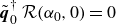 $\tilde {\boldsymbol{q}}^{\dagger }_0 \,\mathcal{R}(\alpha _0,0)=0$
, where
$\tilde {\boldsymbol{q}}^{\dagger }_0 \,\mathcal{R}(\alpha _0,0)=0$
, where $(\boldsymbol{\cdot })^{\dagger }$
represents the Hermitian transpose, with normalisation
$(\boldsymbol{\cdot })^{\dagger }$
represents the Hermitian transpose, with normalisation $\tilde {\boldsymbol{q}}^{\dagger }_0 \,(\mathcal{B}+2\alpha _0 \,\mathcal{V}_{\mathit{xx}})\hat {\boldsymbol{q}}_0=1$
. At
$\tilde {\boldsymbol{q}}^{\dagger }_0 \,(\mathcal{B}+2\alpha _0 \,\mathcal{V}_{\mathit{xx}})\hat {\boldsymbol{q}}_0=1$
. At $(\alpha _0,0)$
,
$(\alpha _0,0)$
, $\mathcal{R}$
is singular. Thus, to enforce solvability, we project the first-order perturbation (3.6) onto
$\mathcal{R}$
is singular. Thus, to enforce solvability, we project the first-order perturbation (3.6) onto $\tilde {\boldsymbol{q}}_0$
, yielding the first-order eigenvalue correction
$\tilde {\boldsymbol{q}}_0$
, yielding the first-order eigenvalue correction
 \begin{align} \delta \alpha = Ri \, (\tilde {\boldsymbol{q}}^{\dagger }_0 \, \mathcal{C} \, \hat {\boldsymbol{q}}_0), \quad \text{with} \quad C_0 :=\left .\frac {\partial \alpha }{\partial Ri}\right |_{Ri=0}=\tilde {\boldsymbol{q}}^{\dagger }_0 \, \mathcal{C} \, \hat {\boldsymbol{q}}_0, \end{align}
where $C_0$
is the (complex) first-order eigenvalue sensitivity.
$C_0$
is the (complex) first-order eigenvalue sensitivity.
Finally, the eigenvalue of the buoyant boundary layer, to order $\mathcal{O}(Ri)$
, reads
$\mathcal{O}(Ri)$
, reads
 \begin{align} \alpha = \alpha _0 + C_0 Ri. \end{align}
The first-order eigenfunction correction $\delta \hat {\boldsymbol{q}}$
follows from the first-order perturbation (3.6), subject to the first-order normalisation constraint
$\delta \hat {\boldsymbol{q}}$
follows from the first-order perturbation (3.6), subject to the first-order normalisation constraint $\tilde {\boldsymbol{q}}^{\dagger }_0 \,(\mathcal{B}+2\alpha _0 \,\mathcal{V}_{\mathit{xx}})\,\delta \hat {\boldsymbol{q}} + 2 \,\delta \alpha \,\tilde {\boldsymbol{q}}^{\dagger }_0 \mathcal{V}_{\mathit{xx}}{}\hat {\boldsymbol{q}}_0=0$
. Note that the extension of the first-order perturbation framework to three-dimensional perturbations is discussed in Appendix B.
$\tilde {\boldsymbol{q}}^{\dagger }_0 \,(\mathcal{B}+2\alpha _0 \,\mathcal{V}_{\mathit{xx}})\,\delta \hat {\boldsymbol{q}} + 2 \,\delta \alpha \,\tilde {\boldsymbol{q}}^{\dagger }_0 \mathcal{V}_{\mathit{xx}}{}\hat {\boldsymbol{q}}_0=0$
. Note that the extension of the first-order perturbation framework to three-dimensional perturbations is discussed in Appendix B.
The sensitivity $C_0$
, following the first-order buoyancy operator (3.5), can be reformulated as
$C_0$
, following the first-order buoyancy operator (3.5), can be reformulated as
 \begin{equation} C_0=C_{0,\mathit{OB}}+C_{0,\mathit{NOB}}, \end{equation}
with
 \begin{equation} C_{0,\mathit{OB}}=\dfrac {\rho ^*_\infty }{\Delta \rho ^*}\int _0^{\infty } \tilde {v}_0^{\dagger }\hat {\rho }_0 \, \mathrm{d}y \quad \text{and} \quad C_{0,\mathit{NOB}}=\dfrac {\rho ^*_\infty }{\Delta \rho ^*}\int _0^{\infty } \tilde {T}_0^{\dagger }(\bar {\rho }-1)\hat {v}_0 \, \mathrm{d}y. \end{equation}
The first term $C_{0,\mathit{OB}}$
represents the classical OB buoyancy coupling, while
$C_{0,\mathit{OB}}$
represents the classical OB buoyancy coupling, while $C_{0,\mathit{NOB}}$
accounts for the NOB buoyancy contribution: density variations in the base flow, through
$C_{0,\mathit{NOB}}$
accounts for the NOB buoyancy contribution: density variations in the base flow, through $\bar {\rho }-1$
, modulate the coupling between temperature and wall-normal velocity fluctuations.
$\bar {\rho }-1$
, modulate the coupling between temperature and wall-normal velocity fluctuations.
Importantly, $C_{0,\mathit{OB}}$
directly governs the first-order buoyancy production in the perturbation kinetic-energy budget
$C_{0,\mathit{OB}}$
directly governs the first-order buoyancy production in the perturbation kinetic-energy budget
 \begin{equation} \varTheta = \mathcal{K} + \mathcal{P} + \mathcal{T} + \mathcal{V} + \mathcal{P}_{\boldsymbol{S}}, \end{equation}
where $\mathcal{K}$
represents the temporal evolution,
$\mathcal{K}$
represents the temporal evolution, $\mathcal{P}$
the shear production,
$\mathcal{P}$
the shear production, $\mathcal{T}$
the thermodynamic contributions,
$\mathcal{T}$
the thermodynamic contributions, $\mathcal{V}$
the viscous dissipation and
$\mathcal{V}$
the viscous dissipation and $\mathcal{P}_{\boldsymbol{S}}$
the buoyancy production, with the real part of
$\mathcal{P}_{\boldsymbol{S}}$
the buoyancy production, with the real part of $\varTheta$
giving the spatial amplification rate of the perturbation energy. The full expressions are provided in Appendix E. Specifically, to order
$\varTheta$
giving the spatial amplification rate of the perturbation energy. The full expressions are provided in Appendix E. Specifically, to order $\mathcal{O}(Ri)$
, the net buoyancy production reads
$\mathcal{O}(Ri)$
, the net buoyancy production reads
 \begin{equation} \text{Re}\{\mathcal{P}_{\boldsymbol{S}}\} = - Ri \, \text{Re}\{C_{0,\mathit{OB}}\}, \end{equation}
where the sign determines whether the buoyancy contribution is stabilising or destabilising, and $\text{Re}$
denotes the real part. The overall spatial growth of the perturbation, however, follows from the complete budget (3.11).
$\text{Re}$
denotes the real part. The overall spatial growth of the perturbation, however, follows from the complete budget (3.11).
4. First-order buoyancy correction: ideal gas
In this section, we validate and apply the first-order buoyancy correction derived in § 3 to ideal-gas stratified boundary-layer flows. The accuracy of the first-order correction for buoyancy effects on the TS wave is assessed in § 4.1 for a nearly incompressible (Blasius) boundary layer. Subsequently, § 4.2 examines the parametric variation of the first-order eigenvalue sensitivity $C_0$
across a wide range of Prandtl numbers, Mach numbers and wall-to-free stream temperature ratios, with a particular focus on the
$C_0$
across a wide range of Prandtl numbers, Mach numbers and wall-to-free stream temperature ratios, with a particular focus on the $N$
-factor for transition prediction.
$N$
-factor for transition prediction.
4.1. Neutral curves, growth rates and $N$
-factors
$N$
-factors

(a) Base-flow profiles of streamwise velocity $\bar {u}/u^*_\infty$
, temperature
$\bar {u}/u^*_\infty$
, temperature $\bar {T}^*/T^*_\infty$
and density
$\bar {T}^*/T^*_\infty$
and density $\bar {\rho }^*/\rho ^*_\infty$
for
$\bar {\rho }^*/\rho ^*_\infty$
for $T^*_{{w}}/T^*_\infty =1.01$
over the dimensionless wall-normal coordinate
$T^*_{{w}}/T^*_\infty =1.01$
over the dimensionless wall-normal coordinate $y^*/\delta ^*$
. The black arrow indicates the direction of gravity. The velocity and thermal boundary-layer thicknesses,
$y^*/\delta ^*$
. The black arrow indicates the direction of gravity. The velocity and thermal boundary-layer thicknesses, $\delta _{99}$
and
$\delta _{99}$
and $\delta _t$
, are indicated, respectively. (b) Neutral-stability curves in the
$\delta _t$
, are indicated, respectively. (b) Neutral-stability curves in the $\textit{Re}$
–
$\textit{Re}$
– $F$
plane for
$F$
plane for $T^*_{{w}}/T^*_\infty =1.01$
at
$T^*_{{w}}/T^*_\infty =1.01$
at $Ri=[-0.04,0,0.04]$
. The black dotted line shows the neutral stability of the Blasius profile.
$Ri=[-0.04,0,0.04]$
. The black dotted line shows the neutral stability of the Blasius profile.

We consider a flat-plate boundary layer with free stream Mach number $M_\infty =0.01$
and
$M_\infty =0.01$
and $\textit{Pr}_\infty =1$
. A minimal wall-to-free stream temperature difference (ratio
$\textit{Pr}_\infty =1$
. A minimal wall-to-free stream temperature difference (ratio $T^*_{{w}}/T^*_\infty =1.01$
, i.e.
$T^*_{{w}}/T^*_\infty =1.01$
, i.e. $|\Delta \rho ^*/\rho ^*_\infty |=0.01$
) introduces mild stratification while keeping the flow nearly incompressible. The reference case corresponds to the neutrally buoyant boundary layer with source-term vector
$|\Delta \rho ^*/\rho ^*_\infty |=0.01$
) introduces mild stratification while keeping the flow nearly incompressible. The reference case corresponds to the neutrally buoyant boundary layer with source-term vector $\boldsymbol{S}=0$
(see (2.5)). The base flow is shown in figure 1(a) and the corresponding neutral-stability curve (
$\boldsymbol{S}=0$
(see (2.5)). The base flow is shown in figure 1(a) and the corresponding neutral-stability curve ( $\mathrm{Im}\{\alpha _0\}=0$
) in the
$\mathrm{Im}\{\alpha _0\}=0$
) in the $\textit{Re}$
–
$\textit{Re}$
– $F$
plane is presented in figure 1(b), where
$F$
plane is presented in figure 1(b), where $F=\omega ^*\mu ^*_\infty /(\rho ^*_\infty u^{*2}_\infty )$
denotes the dimensionless frequency. Stable (
$F=\omega ^*\mu ^*_\infty /(\rho ^*_\infty u^{*2}_\infty )$
denotes the dimensionless frequency. Stable ( $Ri\gt 0$
) and unstable (
$Ri\gt 0$
) and unstable ( $Ri\lt 0$
) stratification use the same base flow (figure 1
a) but opposite gravity directions, resulting in a different Richardson number
$Ri\lt 0$
) stratification use the same base flow (figure 1
a) but opposite gravity directions, resulting in a different Richardson number $Ri$
(see (2.4)). Flipping the gravity direction changes the sign of
$Ri$
(see (2.4)). Flipping the gravity direction changes the sign of $Ri$
without modifying the base flow, thereby isolating the buoyancy effect on instability. Positive
$Ri$
without modifying the base flow, thereby isolating the buoyancy effect on instability. Positive $Ri$
stabilises the TS wave as reported by Parente et al. (Reference Parente, Robinet, de Palma and Cherubini2020), whereas
$Ri$
stabilises the TS wave as reported by Parente et al. (Reference Parente, Robinet, de Palma and Cherubini2020), whereas $Ri\lt 0$
promotes instability. The neutral curve for the neutrally buoyant boundary layer (
$Ri\lt 0$
promotes instability. The neutral curve for the neutrally buoyant boundary layer ( $Ri=0$
) slightly deviates from that of the incompressible (Blasius) boundary layer due to non-uniform temperature-dependent fluid viscosity (see also Wall & Wilson Reference Wall and Wilson1997).
$Ri=0$
) slightly deviates from that of the incompressible (Blasius) boundary layer due to non-uniform temperature-dependent fluid viscosity (see also Wall & Wilson Reference Wall and Wilson1997).
Contours of (a) $\mathrm{Im}\{C_0\}$
and (b)
$\mathrm{Im}\{C_0\}$
and (b) $\mathrm{Re}\{C_0\}$
in the
$\mathrm{Re}\{C_0\}$
in the $\textit{Re}$
–
$\textit{Re}$
– $F$
plane. The black solid line indicates the neutral-stability curve where
$F$
plane. The black solid line indicates the neutral-stability curve where $\mathrm{Im}\{\alpha _0\}=0$
.
$\mathrm{Im}\{\alpha _0\}=0$
.

The sensitivity of the first-order buoyancy correction (3.7) is governed by $C_0$
. Figure 2 displays its imaginary (
$C_0$
. Figure 2 displays its imaginary ( $\mathrm{Im}\{C_0\}$
) and real (
$\mathrm{Im}\{C_0\}$
) and real ( ${\rm Re}\{C_0\}$
) parts in panels (a) and (b), respectively. We evaluate
${\rm Re}\{C_0\}$
) parts in panels (a) and (b), respectively. We evaluate $C_0$
at each
$C_0$
at each $({Re}, F)$
. Because
$({Re}, F)$
. Because $C_0$
is computed for the neutrally buoyant case (subscript
$C_0$
is computed for the neutrally buoyant case (subscript $0$
,
$0$
, $Ri=0$
), it is independent of the stratification level; within the neutral-stability curve its contours vary only weakly with
$Ri=0$
), it is independent of the stratification level; within the neutral-stability curve its contours vary only weakly with $ \textit{Re}$
and
$ \textit{Re}$
and $F$
, especially
$F$
, especially ${\rm Re}\{C_0\}$
. Consequently, it is not necessary to re-solve the eigenvalue problem (3.3) at every
${\rm Re}\{C_0\}$
. Consequently, it is not necessary to re-solve the eigenvalue problem (3.3) at every $(Re, F)$
to apply the first-order correction. Instead, we adopt a single representative value
$(Re, F)$
to apply the first-order correction. Instead, we adopt a single representative value $\bar {C}_0$
, defined as the arithmetic mean of
$\bar {C}_0$
, defined as the arithmetic mean of $C_0$
inside the neutral curve, i.e.
$C_0$
inside the neutral curve, i.e. $\bar {C}_0 = 1/A \iint _{{U}_{\mathit{\alpha }}} C_0(Re,F) \, \mathrm{d}{Re} \, \mathrm{d}F$
, where
$\bar {C}_0 = 1/A \iint _{{U}_{\mathit{\alpha }}} C_0(Re,F) \, \mathrm{d}{Re} \, \mathrm{d}F$
, where $U_{\mathit{\alpha }}$
denotes the unstable region enclosed by the neutral curve and
$U_{\mathit{\alpha }}$
denotes the unstable region enclosed by the neutral curve and $A$
is its area. Substituting
$A$
is its area. Substituting $\bar {C}_0$
into the first-order correction (3.8) corrects the stability of the neutrally buoyant reference case by the factor
$\bar {C}_0$
into the first-order correction (3.8) corrects the stability of the neutrally buoyant reference case by the factor $\bar {C}_0 Ri$
. Note that in this weakly stratified case (figure 1
a), the NOB contribution in the buoyancy sensitivity (3.9) is absent, thus
$\bar {C}_0 Ri$
. Note that in this weakly stratified case (figure 1
a), the NOB contribution in the buoyancy sensitivity (3.9) is absent, thus $C_0 \approx C_{0,\mathit{OB}}$
.
$C_0 \approx C_{0,\mathit{OB}}$
.
Neutral-stability curves in the $\textit{Re}$
–
$\textit{Re}$
– $F$
plane for stably and unstably stratified cases at
$F$
plane for stably and unstably stratified cases at $Ri=[-0.1,-0.04,0.04]$
. Symbols (
$Ri=[-0.1,-0.04,0.04]$
. Symbols ( $\circ$
) show results from the buoyant eigenvalue problem (3.2); solid lines denote the first-order correction (3.8) evaluated with
$\circ$
) show results from the buoyant eigenvalue problem (3.2); solid lines denote the first-order correction (3.8) evaluated with $C_0$
; dotted lines depict the first-order correction (3.8) evaluated with
$C_0$
; dotted lines depict the first-order correction (3.8) evaluated with $\bar {C}_0$
. The neutrally buoyant case at
$\bar {C}_0$
. The neutrally buoyant case at $Ri=0$
is indicated with a black dashed line. The black dash-dotted horizontal line indicates the dimensionless frequency
$Ri=0$
is indicated with a black dashed line. The black dash-dotted horizontal line indicates the dimensionless frequency $F=45\times 10^{-6}$
, at which the growth rate and phase speed are extracted in figure 4. The black pentagram indicates the location at which the eigenfunctions are extracted in Appendix C.
$F=45\times 10^{-6}$
, at which the growth rate and phase speed are extracted in figure 4. The black pentagram indicates the location at which the eigenfunctions are extracted in Appendix C.

We now apply the first-order buoyancy correction (3.8), using both $C_0$
and
$C_0$
and $\bar {C}_0$
, to the neutrally buoyant reference case and, for validation, compare against the buoyant (direct) eigenvalue problem (3.2) for unstably (
$\bar {C}_0$
, to the neutrally buoyant reference case and, for validation, compare against the buoyant (direct) eigenvalue problem (3.2) for unstably ( $Ri=[-0.1,-0.04]$
) and stably (
$Ri=[-0.1,-0.04]$
) and stably ( $Ri=0.04$
) stratified cases. We emphasise that (3.8) requires only a single calculation at
$Ri=0.04$
) stratified cases. We emphasise that (3.8) requires only a single calculation at $Ri=0$
and is then used for moderate
$Ri=0$
and is then used for moderate $Ri$
. For instance, evaluating (3.8) requires only
$Ri$
. For instance, evaluating (3.8) requires only ${\sim} 0.1\,\%$
of the wall-clock time needed to solve the buoyant eigenvalue problem (3.2) with
${\sim} 0.1\,\%$
of the wall-clock time needed to solve the buoyant eigenvalue problem (3.2) with $N_{\mathit{y}}=201$
wall-normal collocation points. In figure 3, the neutral stability is displayed in the
$N_{\mathit{y}}=201$
wall-normal collocation points. In figure 3, the neutral stability is displayed in the $\textit{Re}$
–
$\textit{Re}$
– $F$
plane on double-logarithmic axes. Circles denote solutions of the buoyant eigenvalue problem (3.2), while solid and dotted lines show the first-order correction (3.8) using the local
$F$
plane on double-logarithmic axes. Circles denote solutions of the buoyant eigenvalue problem (3.2), while solid and dotted lines show the first-order correction (3.8) using the local $C_0$
and
$C_0$
and $\bar {C}_0$
, respectively. Using
$\bar {C}_0$
, respectively. Using $C_0$
, excellent agreement of branches I and II is obtained up to
$C_0$
, excellent agreement of branches I and II is obtained up to $Ri=-0.1$
. The averaged
$Ri=-0.1$
. The averaged $\bar {C}_0$
continues to provide a robust prediction of the neutral curve up to
$\bar {C}_0$
continues to provide a robust prediction of the neutral curve up to $Ri=-0.04$
; however, for
$Ri=-0.04$
; however, for $Ri=-0.1$
, the discrepancies in the critical Reynolds number (
$Ri=-0.1$
, the discrepancies in the critical Reynolds number ( $ \textit{Re}_{\textit{crit}}$
), and along branches I and II at low frequencies can exceed
$ \textit{Re}_{\textit{crit}}$
), and along branches I and II at low frequencies can exceed $20\,\%$
. Accordingly,
$20\,\%$
. Accordingly, $\bar {C}_0$
remains valid for weak stratification, whereas for stronger buoyancy effects, nonlinear deviations become significant and the local
$\bar {C}_0$
remains valid for weak stratification, whereas for stronger buoyancy effects, nonlinear deviations become significant and the local $C_0$
is required for accurate stability predictions. The increasing discrepancy at higher
$C_0$
is required for accurate stability predictions. The increasing discrepancy at higher $ \textit{Re}$
follows from the monotonic decrease of
$ \textit{Re}$
follows from the monotonic decrease of $\mathrm{Im}\{C_0\}$
with
$\mathrm{Im}\{C_0\}$
with $ \textit{Re}$
(see figure 2):
$ \textit{Re}$
(see figure 2): $\bar {C}_0$
is dominated by the low-
$\bar {C}_0$
is dominated by the low- $\textit{Re}$
region, where the unstable area is largest due to the viscous nature of the TS instability and where
$\textit{Re}$
region, where the unstable area is largest due to the viscous nature of the TS instability and where $\mathrm{Im}\{C_0\}$
attains its highest values, thereby overestimating the local buoyancy correction at high
$\mathrm{Im}\{C_0\}$
attains its highest values, thereby overestimating the local buoyancy correction at high $ \textit{Re}$
. A comparison of the corresponding eigenfunctions between the buoyant eigenvalue problem (3.2) and the first-order correction (3.8), extracted within the unstable region (indicated by the black pentagram in figure 3), is reported in Appendix C.
$ \textit{Re}$
. A comparison of the corresponding eigenfunctions between the buoyant eigenvalue problem (3.2) and the first-order correction (3.8), extracted within the unstable region (indicated by the black pentagram in figure 3), is reported in Appendix C.
(a) Growth rate and (b) phase speed as functions of $\textit{Re}$
at
$\textit{Re}$
at $F=45 \times 10^{-6}$
for stably and unstably stratified cases at
$F=45 \times 10^{-6}$
for stably and unstably stratified cases at $Ri=[-0.1,-0.04,0.04]$
. Symbols (
$Ri=[-0.1,-0.04,0.04]$
. Symbols ( $\circ$
) show results from the buoyant eigenvalue problem (3.2); solid lines denote the first-order correction (3.8) evaluated with
$\circ$
) show results from the buoyant eigenvalue problem (3.2); solid lines denote the first-order correction (3.8) evaluated with $C_0$
; dotted lines depict the first-order correction (3.8) evaluated with
$C_0$
; dotted lines depict the first-order correction (3.8) evaluated with $\bar {C}_0$
. The neutrally buoyant case at
$\bar {C}_0$
. The neutrally buoyant case at $Ri=0$
is indicated with a black dashed line.
$Ri=0$
is indicated with a black dashed line.

Fixing the frequency at $F=45 \times 10^{-6}$
, indicated by the black dash-dotted horizontal line in figure 3, figure 4 compares the evolution of the growth rate
$F=45 \times 10^{-6}$
, indicated by the black dash-dotted horizontal line in figure 3, figure 4 compares the evolution of the growth rate $\mathrm{Im}\{\alpha \}$
(panel a) and the real part of the phase speed
$\mathrm{Im}\{\alpha \}$
(panel a) and the real part of the phase speed $c_{\mathit{r}}=\omega /{\rm Re}\{\alpha \}$
(panel b) as functions of
$c_{\mathit{r}}=\omega /{\rm Re}\{\alpha \}$
(panel b) as functions of $\textit{Re}$
. Unstable stratification at
$\textit{Re}$
. Unstable stratification at $Ri=-0.1$
yields a maximum growth rate approximately three times larger than that of the neutrally buoyant case
$Ri=-0.1$
yields a maximum growth rate approximately three times larger than that of the neutrally buoyant case $\mathrm{Im}\{\alpha =\alpha _0\}$
(black dashed line). Conversely, stable stratification leads to a reduction in phase speed. Using
$\mathrm{Im}\{\alpha =\alpha _0\}$
(black dashed line). Conversely, stable stratification leads to a reduction in phase speed. Using $C_0$
, the most unstable case at
$C_0$
, the most unstable case at $Ri=-0.1$
is predicted with relative errors of approximately
$Ri=-0.1$
is predicted with relative errors of approximately $5\,\%$
at
$5\,\%$
at $\max \{-\mathrm{Im}\{\alpha \}\}$
and
$\max \{-\mathrm{Im}\{\alpha \}\}$
and $4\,\%$
in the critical Reynolds number
$4\,\%$
in the critical Reynolds number $ \textit{Re}_{\textit{crit}}$
. The largest discrepancies between
$ \textit{Re}_{\textit{crit}}$
. The largest discrepancies between $C_0$
and
$C_0$
and $\bar {C}_0$
occur near
$\bar {C}_0$
occur near $\mathrm{Im}\{\alpha \}=0$
, consistent with figure 3. Notably, for
$\mathrm{Im}\{\alpha \}=0$
, consistent with figure 3. Notably, for $Ri=-0.1$
, the maximum growth rate at
$Ri=-0.1$
, the maximum growth rate at $\textit{Re}\approx 1000$
is accurately captured when using
$\textit{Re}\approx 1000$
is accurately captured when using $\bar {C}_0$
, with a relative error similar to that obtained with
$\bar {C}_0$
, with a relative error similar to that obtained with $C_0$
. A comparable trend in the relative error is seen for
$C_0$
. A comparable trend in the relative error is seen for $c_{\mathit{r}}$
in figure 4(b). Under stronger unstable stratification, the phase speed is well predicted in the vicinity of the largest growth rate
$c_{\mathit{r}}$
in figure 4(b). Under stronger unstable stratification, the phase speed is well predicted in the vicinity of the largest growth rate $\max \{-\mathrm{Im}\{\alpha \}\}$
. For weaker stratification, both first-order corrections based on
$\max \{-\mathrm{Im}\{\alpha \}\}$
. For weaker stratification, both first-order corrections based on $C_0$
and
$C_0$
and $\bar {C}_0$
accurately predict the evolution of
$\bar {C}_0$
accurately predict the evolution of $c_{\mathit{r}}$
.
$c_{\mathit{r}}$
.
In addition to the local amplification shown in figure 4(a), the calculation of the $N$
-factor is essential for practical transition prediction. Using the first-order buoyancy correction (3.8), the
$N$
-factor is essential for practical transition prediction. Using the first-order buoyancy correction (3.8), the $N$
-factor,
$N$
-factor, $N = -\int _{x_0}^{x}\mathrm{Im}\{\alpha \}\,\mathrm{d}x$
for unstably and stably stratified flows can be written as
$N = -\int _{x_0}^{x}\mathrm{Im}\{\alpha \}\,\mathrm{d}x$
for unstably and stably stratified flows can be written as
 \begin{equation} N=N_{\mathit{Ri=0}}+ Ri\, \left .\frac {\partial N}{\partial Ri}\right |_{\mathit{Ri=0}}= -\int _{x_0}^{x}\mathrm{Im}\{\alpha _0\}\,\mathrm{d}x -Ri\int _{x_0}^{x}\mathrm{Im}\{C_0\}\,\mathrm{d}x. \end{equation} $N$
-factor envelopes at
$N$
-factor envelopes at $Ri=[-0.1,-0.04,0,0.04]$
. Symbols (
$Ri=[-0.1,-0.04,0,0.04]$
. Symbols ( $\circ$
) show results from the buoyant eigenvalue problem (3.2); solid lines denote the first-order correction (3.8) evaluated with
$\circ$
) show results from the buoyant eigenvalue problem (3.2); solid lines denote the first-order correction (3.8) evaluated with $C_0$
; dotted lines depict the first-order correction (3.8) evaluated with
$C_0$
; dotted lines depict the first-order correction (3.8) evaluated with $\bar {C}_0$
. The
$\bar {C}_0$
. The $N$
-factor of the neutrally buoyant case is indicated with a black dashed line. The location of maximum amplification rate,
$N$
-factor of the neutrally buoyant case is indicated with a black dashed line. The location of maximum amplification rate, $\max \{-\mathrm{Im}\{\alpha _0\}/{Re}\}$
, is indicated with a black pentagram.
$\max \{-\mathrm{Im}\{\alpha _0\}/{Re}\}$
, is indicated with a black pentagram.

Figure 5 displays the $N$
-factor envelopes obtained from (4.1) using both
$N$
-factor envelopes obtained from (4.1) using both $C_0$
and
$C_0$
and $\bar {C}_0$
, compared with the solution of the buoyant eigenvalue (3.2) for different stratification levels. Note that the
$\bar {C}_0$
, compared with the solution of the buoyant eigenvalue (3.2) for different stratification levels. Note that the $N$
-factor envelope represents, at each streamwise position
$N$
-factor envelope represents, at each streamwise position $x$
, the maximum
$x$
, the maximum $N$
-factor over all frequencies
$N$
-factor over all frequencies $F$
. Unstable stratification yields significantly higher
$F$
. Unstable stratification yields significantly higher $N$
-factors, consistent with the enhanced growth rates in figure 4(a), leading to earlier transition, while stable stratification delays transition. Note that
$N$
-factors, consistent with the enhanced growth rates in figure 4(a), leading to earlier transition, while stable stratification delays transition. Note that $N$
-factor predictions do not explicitly consider the role of the initial disturbance amplitude and therefore require calibration with experimental data, which are not yet available for the present stratified flow conditions. Overall, the first-order correction reproduces the
$N$
-factor predictions do not explicitly consider the role of the initial disturbance amplitude and therefore require calibration with experimental data, which are not yet available for the present stratified flow conditions. Overall, the first-order correction reproduces the $N$
-factor well, with the most accurate prediction obtained when using
$N$
-factor well, with the most accurate prediction obtained when using $C_0$
rather than
$C_0$
rather than $\bar {C}_0$
. The latter is observed to be accurate for weak stratification near the maximum of the amplification rate, defined as
$\bar {C}_0$
. The latter is observed to be accurate for weak stratification near the maximum of the amplification rate, defined as $\max \{-\mathrm{Im}\{\alpha _0\}/\textit{Re}\}$
(neutrally buoyant case) and indicated by a pentagram in figure 5 following Mack (Reference Mack1984). This low-
$\max \{-\mathrm{Im}\{\alpha _0\}/\textit{Re}\}$
(neutrally buoyant case) and indicated by a pentagram in figure 5 following Mack (Reference Mack1984). This low- $\textit{Re}$
amplification maximum is typical of TS modes and, due to the integral nature of the
$\textit{Re}$
amplification maximum is typical of TS modes and, due to the integral nature of the $N$
-factor, the region around this peak dominates the integral amplification. Consequently, evaluating
$N$
-factor, the region around this peak dominates the integral amplification. Consequently, evaluating $C_0$
at the location of
$C_0$
at the location of $\max \{-\mathrm{Im}\{\alpha _0\}/\textit{Re}\}$
captures the dominant buoyancy contribution to the
$\max \{-\mathrm{Im}\{\alpha _0\}/\textit{Re}\}$
captures the dominant buoyancy contribution to the $N$
-factor envelope. Consistent with this interpretation, the buoyancy sensitivity
$N$
-factor envelope. Consistent with this interpretation, the buoyancy sensitivity $\partial N/\partial Ri|_{\mathit{Ri=0}}$
is largest at low
$\partial N/\partial Ri|_{\mathit{Ri=0}}$
is largest at low $\textit{Re}$
. Therefore,
$\textit{Re}$
. Therefore, $N$
-factor envelopes obtained by evaluating
$N$
-factor envelopes obtained by evaluating $C_0$
at
$C_0$
at $\max \{-\mathrm{Im}\{\alpha _0\}/\textit{Re}\}$
agree well with the actual
$\max \{-\mathrm{Im}\{\alpha _0\}/\textit{Re}\}$
agree well with the actual $N$
-factor (buoyant eigenvalue problem) near the amplification maximum (not shown), but become less accurate farther downstream, where the averaged
$N$
-factor (buoyant eigenvalue problem) near the amplification maximum (not shown), but become less accurate farther downstream, where the averaged $\bar {C}_0$
performs better.
$\bar {C}_0$
performs better.
4.2. Base-flow variation: buoyancy sensitivity
After verifying the first-order buoyancy correction on a representative base flow, we examine its behaviour across different flow parameters, i.e. Mach number $M_\infty$
, Prandtl number
$M_\infty$
, Prandtl number $\textit{Pr}_\infty$
and wall-to-free stream temperature ratios
$\textit{Pr}_\infty$
and wall-to-free stream temperature ratios $T^*_{{w}}/T^*_\infty$
, which modify the base-flow density profile and hence the buoyancy variation in
$T^*_{{w}}/T^*_\infty$
, which modify the base-flow density profile and hence the buoyancy variation in $\delta \mathcal{A}$
(see the first-order buoyancy operator (3.5)). Figures 6(a) and 6(b) show
$\delta \mathcal{A}$
(see the first-order buoyancy operator (3.5)). Figures 6(a) and 6(b) show $\mathrm{Im}\{\bar {C}_0\}$
, with
$\mathrm{Im}\{\bar {C}_0\}$
, with $\bar {C}_0$
computed analogously to figure 3. Note that the black dashed line marks
$\bar {C}_0$
computed analogously to figure 3. Note that the black dashed line marks $\mathrm{Im}\{\alpha _0\}=0$
; thus, in that region (at large
$\mathrm{Im}\{\alpha _0\}=0$
; thus, in that region (at large $\textit{Pr}_\infty$
with
$\textit{Pr}_\infty$
with $T^*_{{w}}/T^*_{\mathit{\infty }} \lesssim 0.88$
), no unstable
$T^*_{{w}}/T^*_{\mathit{\infty }} \lesssim 0.88$
), no unstable $\alpha _0$
exists in the
$\alpha _0$
exists in the $(\textit{Re},F)$
plane up to
$(\textit{Re},F)$
plane up to $\textit{Re}=2000$
. In such cases,
$\textit{Re}=2000$
. In such cases, $C_0$
is evaluated locally for the stable TS mode. In panel (a) at
$C_0$
is evaluated locally for the stable TS mode. In panel (a) at $M_\infty =0.01$
,
$M_\infty =0.01$
, $\mathrm{Im}\{\bar {C}_0\}$
is strongly dependent on
$\mathrm{Im}\{\bar {C}_0\}$
is strongly dependent on $\textit{Pr}_\infty$
. After peaking near
$\textit{Pr}_\infty$
. After peaking near $\textit{Pr}_\infty \simeq 7$
(i.e. water), the buoyancy sensitivity decreases monotonically regardless of
$\textit{Pr}_\infty \simeq 7$
(i.e. water), the buoyancy sensitivity decreases monotonically regardless of $T^*_{{w}}/T^*_\infty$
and eventually, for
$T^*_{{w}}/T^*_\infty$
and eventually, for $\textit{Pr}_\infty \gtrsim 70$
(e.g. oil), changes sign. This sign reversal indicates that the role of buoyancy on modal stability switches at high
$\textit{Pr}_\infty \gtrsim 70$
(e.g. oil), changes sign. This sign reversal indicates that the role of buoyancy on modal stability switches at high $\textit{Pr}_\infty$
: for a given sign of
$\textit{Pr}_\infty$
: for a given sign of $Ri$
, flow configurations that are destabilising at low
$Ri$
, flow configurations that are destabilising at low $\textit{Pr}_\infty$
become stabilising at high
$\textit{Pr}_\infty$
become stabilising at high $\textit{Pr}_\infty$
, and vice versa. This non-monotonic dependence of
$\textit{Pr}_\infty$
, and vice versa. This non-monotonic dependence of $\mathrm{Im}\{\bar {C}_0\}$
on
$\mathrm{Im}\{\bar {C}_0\}$
on $\textit{Pr}_\infty$
reflects the mechanism identified by Parente et al. (Reference Parente, Robinet, de Palma and Cherubini2020): increasing
$\textit{Pr}_\infty$
reflects the mechanism identified by Parente et al. (Reference Parente, Robinet, de Palma and Cherubini2020): increasing $\textit{Pr}_\infty$
reduces thermal diffusion, altering the phase between density and velocity perturbations – stabilising the flow through buoyancy effects at low
$\textit{Pr}_\infty$
reduces thermal diffusion, altering the phase between density and velocity perturbations – stabilising the flow through buoyancy effects at low $\textit{Pr}_\infty$
and destabilising it at high
$\textit{Pr}_\infty$
and destabilising it at high $\textit{Pr}_\infty$
. In contrast, the sensitivity to variations in
$\textit{Pr}_\infty$
. In contrast, the sensitivity to variations in $T^*_{{w}}/T^*_\infty$
is small. A similar behaviour holds in figure 6(b) for
$T^*_{{w}}/T^*_\infty$
is small. A similar behaviour holds in figure 6(b) for $M_\infty \lesssim 0.1$
; at higher
$M_\infty \lesssim 0.1$
; at higher $M_\infty$
, compressibility increases
$M_\infty$
, compressibility increases $\mathrm{Im}\{\bar {C}_0\}$
, enhancing TS growth under unstable stratification. Nevertheless, buoyancy effects remain most significant in the low-Mach-number regime, where compressibility effects are weak and stratification effects are most pronounced.
$\mathrm{Im}\{\bar {C}_0\}$
, enhancing TS growth under unstable stratification. Nevertheless, buoyancy effects remain most significant in the low-Mach-number regime, where compressibility effects are weak and stratification effects are most pronounced.
Contours of (a,b) $\mathrm{Im}\{\bar {C}_0\}$
and (c,d)
$\mathrm{Im}\{\bar {C}_0\}$
and (c,d) ${\rm Re}\{\bar {C}_0\}$
in the (a,c)
${\rm Re}\{\bar {C}_0\}$
in the (a,c) $T^*_{{w}}/T^*_{\mathit{\infty }}$
–
$T^*_{{w}}/T^*_{\mathit{\infty }}$
– $\textit{Pr}_{\mathit{\infty }}$
plane at
$\textit{Pr}_{\mathit{\infty }}$
plane at $M_{\mathit{\infty }}=0.01$
and in the (b,d)
$M_{\mathit{\infty }}=0.01$
and in the (b,d) $M_\infty$
–
$M_\infty$
– $\textit{Pr}_\infty$
plane at
$\textit{Pr}_\infty$
plane at $T^*_{{w}}/T^*_{\mathit{\infty }}=1.01$
. In panels (a,c), the region enclosed by the black dashed line
$T^*_{{w}}/T^*_{\mathit{\infty }}=1.01$
. In panels (a,c), the region enclosed by the black dashed line $\mathrm{Im}\{\alpha _0\}=0$
corresponds to
$\mathrm{Im}\{\alpha _0\}=0$
corresponds to $\max \{-\mathrm{Im}\{\alpha _0\}\}\lt 0$
(stable TS mode). The white star indicates the base-flow conditions of § 4.1. In panels (a,c), when
$\max \{-\mathrm{Im}\{\alpha _0\}\}\lt 0$
(stable TS mode). The white star indicates the base-flow conditions of § 4.1. In panels (a,c), when $T^*_{{w}}/T^*_{\mathit{\infty }}=1$
,
$T^*_{{w}}/T^*_{\mathit{\infty }}=1$
, $Ri=0$
. The black solid line indicates
$Ri=0$
. The black solid line indicates $\mathrm{Im}\{\bar {C}_0\}=0$
in panels (a,b) and
$\mathrm{Im}\{\bar {C}_0\}=0$
in panels (a,b) and ${\rm Re}\{\bar {C}_0\}=0$
in panels (c,d). The black regions in panels (b,d) correspond to values outside the colourbar range, namely
${\rm Re}\{\bar {C}_0\}=0$
in panels (c,d). The black regions in panels (b,d) correspond to values outside the colourbar range, namely $\mathrm{Im}\{\bar {C}_0\}\gt 0.3$
in panel (b) and
$\mathrm{Im}\{\bar {C}_0\}\gt 0.3$
in panel (b) and ${\rm Re}\{\bar {C}_0\}\gt 0.2$
in panel (d).
${\rm Re}\{\bar {C}_0\}\gt 0.2$
in panel (d).

Figures 6(c) and 6(d) show the contours of the real part of the buoyancy sensitivity, ${\rm Re}\{\bar {C}_0\}$
. This quantity governs the buoyancy-induced phase-speed modification,
${\rm Re}\{\bar {C}_0\}$
. This quantity governs the buoyancy-induced phase-speed modification, $\delta c_{\mathit{r}}=-\omega\,{\rm Re}\{C_0\}Ri/{\rm Re}\{\alpha _0\}^2$
, and determines the net buoyancy-production term in the perturbation kinetic-energy budget; see (3.12). The dependence of
$\delta c_{\mathit{r}}=-\omega\,{\rm Re}\{C_0\}Ri/{\rm Re}\{\alpha _0\}^2$
, and determines the net buoyancy-production term in the perturbation kinetic-energy budget; see (3.12). The dependence of ${\rm Re}\{\bar {C}_0\}$
on
${\rm Re}\{\bar {C}_0\}$
on $T^*_{{w}}/T^*_\infty$
(panel c) and
$T^*_{{w}}/T^*_\infty$
(panel c) and $M_\infty$
(panel d) is similar to that observed in figures 6(a) and 6(b), but a distinct behaviour emerges with increasing
$M_\infty$
(panel d) is similar to that observed in figures 6(a) and 6(b), but a distinct behaviour emerges with increasing $\textit{Pr}_\infty$
. The locus
$\textit{Pr}_\infty$
. The locus ${\rm Re}\{\bar {C}_0\}=0$
lies near
${\rm Re}\{\bar {C}_0\}=0$
lies near $\textit{Pr}_\infty \approx \mathcal{O}(10)$
, indicating the region where buoyancy switches from decreasing to increasing phase speed. At low
$\textit{Pr}_\infty \approx \mathcal{O}(10)$
, indicating the region where buoyancy switches from decreasing to increasing phase speed. At low $\textit{Pr}_\infty$
, where thermal diffusion dominates, buoyancy decreases the phase speed for stable stratification (
$\textit{Pr}_\infty$
, where thermal diffusion dominates, buoyancy decreases the phase speed for stable stratification ( $Ri\gt 0$
), whereas at high
$Ri\gt 0$
), whereas at high $\textit{Pr}_\infty$
where
$\textit{Pr}_\infty$
where ${\rm Re}\{\bar {C}_0\}\lt 0$
, buoyancy increases the phase speed under stable stratification. Regarding the buoyancy-production term
${\rm Re}\{\bar {C}_0\}\lt 0$
, buoyancy increases the phase speed under stable stratification. Regarding the buoyancy-production term $\mathcal{P}_{\boldsymbol{S}}$
, the sign change of
$\mathcal{P}_{\boldsymbol{S}}$
, the sign change of ${\rm Re}\{\bar {C}_0\}$
at high
${\rm Re}\{\bar {C}_0\}$
at high $\textit{Pr}_\infty$
causes the net buoyancy production (3.12) to become negative. Consequently, for unstable stratification (
$\textit{Pr}_\infty$
causes the net buoyancy production (3.12) to become negative. Consequently, for unstable stratification ( $Ri\lt 0$
), we have
$Ri\lt 0$
), we have ${\rm Re}\{\mathcal{P}_{\boldsymbol{S}}\}\lt 0$
, indicating that buoyancy has a stabilising effect on the perturbation kinetic-energy budget (3.11). However, figures 6(a) and 6(b) show that
${\rm Re}\{\mathcal{P}_{\boldsymbol{S}}\}\lt 0$
, indicating that buoyancy has a stabilising effect on the perturbation kinetic-energy budget (3.11). However, figures 6(a) and 6(b) show that $\mathrm{Im}\{\bar {C}_0\}$
is higher around
$\mathrm{Im}\{\bar {C}_0\}$
is higher around $\textit{Pr}_\infty =\mathcal{O}(10)$
than at
$\textit{Pr}_\infty =\mathcal{O}(10)$
than at $\textit{Pr}_\infty =\mathcal{O}(1)$
. This enhanced destabilisation arises ultimately from the larger thermodynamic term
$\textit{Pr}_\infty =\mathcal{O}(1)$
. This enhanced destabilisation arises ultimately from the larger thermodynamic term $\mathcal{T}$
in the perturbation kinetic-energy budget (3.11) (not shown here), which is driven by stronger temperature fluctuations associated with the thinner thermal boundary layer, in agreement with Parente et al. (Reference Parente, Robinet, de Palma and Cherubini2020).
$\mathcal{T}$
in the perturbation kinetic-energy budget (3.11) (not shown here), which is driven by stronger temperature fluctuations associated with the thinner thermal boundary layer, in agreement with Parente et al. (Reference Parente, Robinet, de Palma and Cherubini2020).
Contours of (a,b) $N$
-factor envelope and (c,d) relative error
$N$
-factor envelope and (c,d) relative error $\varepsilon =|(N-\bar {N})/N|$
(in percentage), evaluated at
$\varepsilon =|(N-\bar {N})/N|$
(in percentage), evaluated at $\textit{Re}=1000$
. (a,c)
$\textit{Re}=1000$
. (a,c) $T^*_{{w}}/T^*_{\mathit{\infty }}$
–
$T^*_{{w}}/T^*_{\mathit{\infty }}$
– $\textit{Pr}_{\mathit{\infty }}$
plane at
$\textit{Pr}_{\mathit{\infty }}$
plane at $M_{\mathit{\infty }}=0.01$
; (b,d)
$M_{\mathit{\infty }}=0.01$
; (b,d) $M_\infty$
–
$M_\infty$
– $\textit{Pr}_\infty$
plane at
$\textit{Pr}_\infty$
plane at $T^*_{{w}}/T^*_{\mathit{\infty }}=1.01$
. We use
$T^*_{{w}}/T^*_{\mathit{\infty }}=1.01$
. We use $|Ri|=0.04$
with gravity directed towards the wall (
$|Ri|=0.04$
with gravity directed towards the wall ( $e_y=-1$
). In panels (a,c), the grey region corresponds to
$e_y=-1$
). In panels (a,c), the grey region corresponds to $N=0$
; note that
$N=0$
; note that $Ri=0$
when
$Ri=0$
when $T^*_{{w}}/T^*_{\mathit{\infty }}=1$
. The white star indicates the base-flow conditions of § 4.1. The black dashed line indicates
$T^*_{{w}}/T^*_{\mathit{\infty }}=1$
. The white star indicates the base-flow conditions of § 4.1. The black dashed line indicates $N=8$
in panels (a,b).
$N=8$
in panels (a,b).

Figures 7(a) and 7(b) show contours of the $N$
-factor envelope at
$N$
-factor envelope at $\textit{Re}=1000$
, computed as
$\textit{Re}=1000$
, computed as $N=\int ^x_{x_0}-\mathrm{Im}\{\alpha \}\,\mathrm{d}x$
from the buoyant eigenvalue problem (3.2). Panel (a) presents the results in the
$N=\int ^x_{x_0}-\mathrm{Im}\{\alpha \}\,\mathrm{d}x$
from the buoyant eigenvalue problem (3.2). Panel (a) presents the results in the $T^*_{{w}}/T^*_\infty$
–
$T^*_{{w}}/T^*_\infty$
– $\textit{Pr}_\infty$
plane at
$\textit{Pr}_\infty$
plane at $M_\infty =0.01$
, while panel (b) shows the
$M_\infty =0.01$
, while panel (b) shows the $M_\infty$
–
$M_\infty$
– $\textit{Pr}_\infty$
plane at
$\textit{Pr}_\infty$
plane at $T^*_{{w}}/T^*_\infty =1.01$
. We set
$T^*_{{w}}/T^*_\infty =1.01$
. We set $|Ri|=0.04$
with gravity directed towards the wall (
$|Ri|=0.04$
with gravity directed towards the wall ( $e_y=-1$
). For wall cooling (
$e_y=-1$
). For wall cooling ( $T^*_{{w}}/T^*_\infty \lt 1$
), the colder, denser fluid lies at the wall, yielding stable stratification
$T^*_{{w}}/T^*_\infty \lt 1$
), the colder, denser fluid lies at the wall, yielding stable stratification $Ri\gt 0$
. Conversely, wall heating (
$Ri\gt 0$
. Conversely, wall heating ( $T^*_{{w}}/T^*_\infty \gt 1$
) produces unstable stratification (
$T^*_{{w}}/T^*_\infty \gt 1$
) produces unstable stratification ( $Ri\lt 0$
) with hotter, lighter fluid at the wall. For
$Ri\lt 0$
) with hotter, lighter fluid at the wall. For $T^*_{{w}}/T^*_\infty \lt 1$
, wall cooling stabilises, as expected, the TS mode (see also
$T^*_{{w}}/T^*_\infty \lt 1$
, wall cooling stabilises, as expected, the TS mode (see also $\mathrm{Im}\{\alpha _0\}=0$
in figure 6
a), and this effect is further enhanced by stable stratification (
$\mathrm{Im}\{\alpha _0\}=0$
in figure 6
a), and this effect is further enhanced by stable stratification ( $Ri=0.04$
), leading to an extended region of complete stabilisation (
$Ri=0.04$
), leading to an extended region of complete stabilisation ( $N=0$
). In comparison, for a neutrally buoyant case, the wall-to-free stream temperature ratio required to achieve
$N=0$
). In comparison, for a neutrally buoyant case, the wall-to-free stream temperature ratio required to achieve $N=0$
would be
$N=0$
would be $T^*_{{w}}/T^*_\infty \approx 0.92$
at
$T^*_{{w}}/T^*_\infty \approx 0.92$
at $\textit{Pr}_\infty \approx 10$
. For
$\textit{Pr}_\infty \approx 10$
. For $T^*_{{w}}/T^*_\infty \gt 1$
, unstable stratification (
$T^*_{{w}}/T^*_\infty \gt 1$
, unstable stratification ( $Ri=-0.04$
) substantially increases the
$Ri=-0.04$
) substantially increases the $N$
-factor, particularly at
$N$
-factor, particularly at $\textit{Pr}_\infty =\mathcal{O}(1)$
, where the buoyancy sensitivity peaks (see figure 6
a). For
$\textit{Pr}_\infty =\mathcal{O}(1)$
, where the buoyancy sensitivity peaks (see figure 6
a). For $T^*_{{w}}/T^*_\infty =1.2$
and
$T^*_{{w}}/T^*_\infty =1.2$
and $\textit{Pr}_\infty \approx 10$
, the neutrally buoyant boundary layer would exhibit an
$\textit{Pr}_\infty \approx 10$
, the neutrally buoyant boundary layer would exhibit an $N$
-factor approximately
$N$
-factor approximately $40\,\%$
lower. Panel (b) shows that
$40\,\%$
lower. Panel (b) shows that $N$
is nearly insensitive to
$N$
is nearly insensitive to $M_\infty$
in the low-Mach-number regime (
$M_\infty$
in the low-Mach-number regime ( $M_\infty \lesssim 0.1$
), but exceeds
$M_\infty \lesssim 0.1$
), but exceeds $40$
in the high-
$40$
in the high- $\textit{Pr}_\infty$
, moderate-
$\textit{Pr}_\infty$
, moderate- $M_\infty$
region. For instance, at
$M_\infty$
region. For instance, at $M_\infty =0.2$
and
$M_\infty =0.2$
and $\textit{Pr}_\infty \approx 100$
, the unstably stratified boundary layer (
$\textit{Pr}_\infty \approx 100$
, the unstably stratified boundary layer ( $Ri=-0.04$
) reaches an
$Ri=-0.04$
) reaches an $N$
-factor almost eight times larger than the neutrally buoyant case.
$N$
-factor almost eight times larger than the neutrally buoyant case.
The accuracy of the first-order buoyancy correction when using $\bar {C}_0$
is assessed through the relative
$\bar {C}_0$
is assessed through the relative $N$
-factor error
$N$
-factor error $\varepsilon =|(N-\bar {N})/N|$
, shown in figures 7(c) and 7(d). The
$\varepsilon =|(N-\bar {N})/N|$
, shown in figures 7(c) and 7(d). The $N$
-factors are extracted from the corresponding envelope at
$N$
-factors are extracted from the corresponding envelope at $\textit{Re}=1000$
, where
$\textit{Re}=1000$
, where $N$
denotes the
$N$
denotes the $N$
-factor from the buoyant eigenvalue problem (3.2) (cf. figures 7
a and 7
b) and
$N$
-factor from the buoyant eigenvalue problem (3.2) (cf. figures 7
a and 7
b) and $\bar {N}$
is computed using
$\bar {N}$
is computed using $\bar {C}_0$
via the first-order correction of the
$\bar {C}_0$
via the first-order correction of the $N$
-factor (4.1). Across the entire
$N$
-factor (4.1). Across the entire $\textit{Pr}_\infty$
and
$\textit{Pr}_\infty$
and $T^*_{{w}}/T^*_\infty$
ranges considered, the
$T^*_{{w}}/T^*_\infty$
ranges considered, the $\bar {C}_0$
-based first-order buoyancy correction reproduces the integral amplification well, with typical errors below
$\bar {C}_0$
-based first-order buoyancy correction reproduces the integral amplification well, with typical errors below $5\,\%$
. However, as compressibility increases (
$5\,\%$
. However, as compressibility increases ( $M_\infty \gtrsim 0.1$
),
$M_\infty \gtrsim 0.1$
), $\varepsilon$
rises substantially, exceeding
$\varepsilon$
rises substantially, exceeding $50\,\%$
in some regions. This indicates that higher-order buoyancy effects become non-negligible at moderate Mach numbers, such that the first-order perturbation theory itself becomes insufficient, and the buoyant eigenvalue problem (3.2) must be solved at each
$50\,\%$
in some regions. This indicates that higher-order buoyancy effects become non-negligible at moderate Mach numbers, such that the first-order perturbation theory itself becomes insufficient, and the buoyant eigenvalue problem (3.2) must be solved at each $Ri$
.
$Ri$
.
5. First-order buoyancy correction: supercritical fluids
Beyond the ideal-gas regime explored in § 4, we apply the first-order perturbation theory to the non-ideal-gas regime of fluids at supercritical pressure. In the vicinity of the critical point, strong density variations ( $\Delta \rho ^*/\rho ^*_\infty \approx \mathcal{O}(1)$
) across the boundary layer become extremely important (Wang et al. Reference Wang, He, Moulinec and Emerson2023; Draskic, Westerweel & Pecnik Reference Draskic, Westerweel and Pecnik2025). Modal instabilities in boundary layers with supercritical fluids have been widely investigated (Ren et al. Reference Ren, Marxen and Pecnik2019; Robinet & Gloerfelt Reference Robinet and Gloerfelt2019), with recent work identifying the crucial role of baroclinic effects in the presence of large density variations (Bugeat et al. Reference Bugeat, Boldini, Hasan and Pecnik2024; Boldini et al. Reference Boldini, Bugeat, Peeters, Kloker and Pecnik2025a
). However, all stability analyses thus far have neglected gravitational effects. Since buoyancy can profoundly affect the modal stability of ideal-gas boundary layers (see § 4) and density stratification in supercritical fluids is orders of magnitude larger, how buoyancy effects alter the instability mechanisms in boundary layers with supercritical fluids remains an open question. Here, we address this by systematically isolating buoyancy contributions through the first-order buoyancy correction.
$\Delta \rho ^*/\rho ^*_\infty \approx \mathcal{O}(1)$
) across the boundary layer become extremely important (Wang et al. Reference Wang, He, Moulinec and Emerson2023; Draskic, Westerweel & Pecnik Reference Draskic, Westerweel and Pecnik2025). Modal instabilities in boundary layers with supercritical fluids have been widely investigated (Ren et al. Reference Ren, Marxen and Pecnik2019; Robinet & Gloerfelt Reference Robinet and Gloerfelt2019), with recent work identifying the crucial role of baroclinic effects in the presence of large density variations (Bugeat et al. Reference Bugeat, Boldini, Hasan and Pecnik2024; Boldini et al. Reference Boldini, Bugeat, Peeters, Kloker and Pecnik2025a
). However, all stability analyses thus far have neglected gravitational effects. Since buoyancy can profoundly affect the modal stability of ideal-gas boundary layers (see § 4) and density stratification in supercritical fluids is orders of magnitude larger, how buoyancy effects alter the instability mechanisms in boundary layers with supercritical fluids remains an open question. Here, we address this by systematically isolating buoyancy contributions through the first-order buoyancy correction.
Base-flow profiles of streamwise velocity $\bar {u}^*/u^*_\infty$
, temperature
$\bar {u}^*/u^*_\infty$
, temperature $\bar {T}^*/T^*_\infty$
, density
$\bar {T}^*/T^*_\infty$
, density $\bar {\rho }^*/\rho ^*_\infty$
and local gradient Richardson number
$\bar {\rho }^*/\rho ^*_\infty$
and local gradient Richardson number $Ri_{\mathit{g}}$
over the dimensionless wall-normal coordinate
$Ri_{\mathit{g}}$
over the dimensionless wall-normal coordinate $y^*/\delta ^*$
. (a) Wall-heating. (b) Wall-cooling. The green dashed line at
$y^*/\delta ^*$
. (a) Wall-heating. (b) Wall-cooling. The green dashed line at $y=y_{\mathit{pc}}$
indicates the location where
$y=y_{\mathit{pc}}$
indicates the location where $\bar {T}^*=T^*_{\mathit{pc}}$
. The black arrow indicates the direction of gravity.
$\bar {T}^*=T^*_{\mathit{pc}}$
. The black arrow indicates the direction of gravity.

We consider two boundary layers with carbon dioxide ( $\text{CO}_2$
) at a supercritical pressure of
$\text{CO}_2$
) at a supercritical pressure of ${80}\,\textrm {bar}$
(critical pressure of
${80}\,\textrm {bar}$
(critical pressure of ${73.9}\,\textrm {bar}$
) under pseudo-boiling conditions (Banuti Reference Banuti2015), where the boundary-layer temperature crosses the pseudo-critical temperature
${73.9}\,\textrm {bar}$
) under pseudo-boiling conditions (Banuti Reference Banuti2015), where the boundary-layer temperature crosses the pseudo-critical temperature $T^*_{\mathit{pc}}$
at which the specific isobaric heat capacity reaches its maximum. The first case features wall heating with
$T^*_{\mathit{pc}}$
at which the specific isobaric heat capacity reaches its maximum. The first case features wall heating with $T^*_\infty /T^*_{\mathit{pc}}=0.90$
and
$T^*_\infty /T^*_{\mathit{pc}}=0.90$
and $T^*_{{w}}/T^*_{\mathit{pc}}=1.05$
at
$T^*_{{w}}/T^*_{\mathit{pc}}=1.05$
at $M_\infty =0.05$
, conditions known to trigger an inflectional inviscid instability (Mode II) (Ren et al. Reference Ren, Marxen and Pecnik2019). The second case involves wall cooling following the study of Ren et al. (Reference Ren, Wu, Mao, Wang and Kloker2025) with
$M_\infty =0.05$
, conditions known to trigger an inflectional inviscid instability (Mode II) (Ren et al. Reference Ren, Marxen and Pecnik2019). The second case involves wall cooling following the study of Ren et al. (Reference Ren, Wu, Mao, Wang and Kloker2025) with $T^*_\infty /T^*_{\mathit{pc}}=1.04$
and
$T^*_\infty /T^*_{\mathit{pc}}=1.04$
and $T^*_{{w}}/T^*_{\mathit{pc}}=0.975$
at
$T^*_{{w}}/T^*_{\mathit{pc}}=0.975$
at $M_\infty =0.2$
, which produces a similar inflectional inviscid mode. Base-flow profiles of streamwise velocity
$M_\infty =0.2$
, which produces a similar inflectional inviscid mode. Base-flow profiles of streamwise velocity $\bar {u}^*/u^*_\infty$
, temperature
$\bar {u}^*/u^*_\infty$
, temperature $\bar {T}^*/T^*_\infty$
, density
$\bar {T}^*/T^*_\infty$
, density $\bar {\rho }^*/\rho ^*_\infty$
and local gradient Richardson number
$\bar {\rho }^*/\rho ^*_\infty$
and local gradient Richardson number $Ri_{\mathit{g}} = -g^* (\mathrm{d}\bar {\rho }^*/\mathrm{d}y^*)/ [\rho ^*(\mathrm{d}\bar {u}^*/\mathrm{d}y^*)^2]$
are shown in figure 8 for wall heating (panel a) and wall cooling (panel b). In the wall-heating case at
$Ri_{\mathit{g}} = -g^* (\mathrm{d}\bar {\rho }^*/\mathrm{d}y^*)/ [\rho ^*(\mathrm{d}\bar {u}^*/\mathrm{d}y^*)^2]$
are shown in figure 8 for wall heating (panel a) and wall cooling (panel b). In the wall-heating case at $M_\infty =0.05$
, the temperature profile crosses
$M_\infty =0.05$
, the temperature profile crosses $T^*_{\mathit{pc}}$
at
$T^*_{\mathit{pc}}$
at $y=y_{\mathit{pc}}$
(pseudo-critical point with continuous fluid property change), generating a near-wall vapour-like region with lower density than the free stream (
$y=y_{\mathit{pc}}$
(pseudo-critical point with continuous fluid property change), generating a near-wall vapour-like region with lower density than the free stream ( $|\Delta \rho ^*/\rho ^*_\infty | \approx 0.77$
). This flow configuration produces unstable stratification with
$|\Delta \rho ^*/\rho ^*_\infty | \approx 0.77$
). This flow configuration produces unstable stratification with $Ri=-0.037$
(corresponding to
$Ri=-0.037$
(corresponding to $\textit{Fr}=4.54$
) and a negative
$\textit{Fr}=4.54$
) and a negative $Ri_{\mathit{g}}$
that reaches its minimum at
$Ri_{\mathit{g}}$
that reaches its minimum at $y_{\mathit{pc}}$
, where gradients of thermophysical properties are strongest. Conversely, the wall-cooling case creates a dense liquid-like region near the wall (
$y_{\mathit{pc}}$
, where gradients of thermophysical properties are strongest. Conversely, the wall-cooling case creates a dense liquid-like region near the wall ( $|\Delta \rho ^*/\rho ^*_\infty | \approx 2.21$
), yielding stable stratification with
$|\Delta \rho ^*/\rho ^*_\infty | \approx 2.21$
), yielding stable stratification with $Ri=0.058$
(corresponding to
$Ri=0.058$
(corresponding to $\textit{Fr}=6.22$
) and a positive
$\textit{Fr}=6.22$
) and a positive $Ri_{\mathit{g}}$
throughout the boundary layer (maximum at
$Ri_{\mathit{g}}$
throughout the boundary layer (maximum at $y_{\mathit{pc}}$
). Thus, the large density gradients at the pseudo-critical point
$y_{\mathit{pc}}$
). Thus, the large density gradients at the pseudo-critical point $y_{\mathit{pc}}$
intensify buoyancy effects, which either stabilise the flow (when
$y_{\mathit{pc}}$
intensify buoyancy effects, which either stabilise the flow (when $Ri_{\mathit{g}}\gt 0$
, stable stratification) or further amplify the underlying modal instability (when
$Ri_{\mathit{g}}\gt 0$
, stable stratification) or further amplify the underlying modal instability (when $Ri_{\mathit{g}}\lt 0$
, unstable stratification).
$Ri_{\mathit{g}}\lt 0$
, unstable stratification).
We examine the linear stability of the wall-heating case in figure 9; the wall-cooling case is presented in Appendix D. For both configurations, the most amplified disturbances are two-dimensional at the low Mach numbers considered here ( $M_\infty \leqslant 0.2$
) (Boldini et al. Reference Boldini, Bugeat, Peeters, Kloker and Pecnik2024; Boldini Reference Boldini2026), justifying the two-dimensional framework adopted for the first-order buoyancy correction in § 3. Panel (a) shows neutral-stability curves in the
$M_\infty \leqslant 0.2$
) (Boldini et al. Reference Boldini, Bugeat, Peeters, Kloker and Pecnik2024; Boldini Reference Boldini2026), justifying the two-dimensional framework adopted for the first-order buoyancy correction in § 3. Panel (a) shows neutral-stability curves in the ${\rm Re}$
–
${\rm Re}$
– $F$
plane for two levels of unstable stratification:
$F$
plane for two levels of unstable stratification: $Ri=-0.037$
, corresponding to the base flow in figure 8(a), and
$Ri=-0.037$
, corresponding to the base flow in figure 8(a), and $Ri=-0.1$
, obtained using the same thermodynamic conditions but at
$Ri=-0.1$
, obtained using the same thermodynamic conditions but at $M_\infty =0.03$
. Unstable stratification shifts the neutral curve towards lower
$M_\infty =0.03$
. Unstable stratification shifts the neutral curve towards lower ${\rm Re}$
, promoting earlier instability. The background contours of
${\rm Re}$
, promoting earlier instability. The background contours of $\mathrm{Im}\{C_0\}$
(panel a) vary strongly within the neutral curve, reflecting the sharp pseudo-boiling-induced gradients that locally modulate buoyancy sensitivity. Consequently, the arithmetic mean
$\mathrm{Im}\{C_0\}$
(panel a) vary strongly within the neutral curve, reflecting the sharp pseudo-boiling-induced gradients that locally modulate buoyancy sensitivity. Consequently, the arithmetic mean $\mathrm{Im}\{\bar {C}_0\}$
, as in figure 2, is not representative under such strong variable-property conditions; the first-order buoyancy correction (3.8) with
$\mathrm{Im}\{\bar {C}_0\}$
, as in figure 2, is not representative under such strong variable-property conditions; the first-order buoyancy correction (3.8) with $\mathrm{Im}\{C_0\}$
evaluated locally at each
$\mathrm{Im}\{C_0\}$
evaluated locally at each $(Re,F)$
is required. Using this local evaluation, the first-order buoyancy correction agrees closely with the solution of the buoyant eigenvalue problem (3.2), with deviations in the neutral curve within
$(Re,F)$
is required. Using this local evaluation, the first-order buoyancy correction agrees closely with the solution of the buoyant eigenvalue problem (3.2), with deviations in the neutral curve within $\sim \!3\,\%$
. Panel (b) shows isolines of constant phase speed
$\sim \!3\,\%$
. Panel (b) shows isolines of constant phase speed $c_{\mathit{r}}=0.32$
in the
$c_{\mathit{r}}=0.32$
in the $ \textit{Re}$
–
$ \textit{Re}$
– $F$
plane. The phase speed computed using
$F$
plane. The phase speed computed using ${\rm Re}\{C_0\}$
agrees closely with the solution from the buoyant eigenvalue problem. According to the buoyancy-induced phase-speed modification,
${\rm Re}\{C_0\}$
agrees closely with the solution from the buoyant eigenvalue problem. According to the buoyancy-induced phase-speed modification, $\delta c_{\mathit{r}}=-\omega\,{\rm Re}\{C_0\}Ri/{\rm Re}\{\alpha _0\}^2$
, we obtain
$\delta c_{\mathit{r}}=-\omega\,{\rm Re}\{C_0\}Ri/{\rm Re}\{\alpha _0\}^2$
, we obtain $\delta c_{\mathit{r}}\gt 0$
since
$\delta c_{\mathit{r}}\gt 0$
since ${\rm Re}\{C_0\}\gt 0$
in this case, indicating that unstable stratification increases the phase-speed of the unstable mode (Mode II). These results confirm that the first-order perturbation theory remains valid even when large density variations (
${\rm Re}\{C_0\}\gt 0$
in this case, indicating that unstable stratification increases the phase-speed of the unstable mode (Mode II). These results confirm that the first-order perturbation theory remains valid even when large density variations ( $\Delta \rho ^*/\rho ^*_\infty \approx \mathcal{O}(1)$
) are present under strong non-ideal gas effects, amplifying buoyancy effects near the pseudo-critical point. The key requirement is the local evaluation of
$\Delta \rho ^*/\rho ^*_\infty \approx \mathcal{O}(1)$
) are present under strong non-ideal gas effects, amplifying buoyancy effects near the pseudo-critical point. The key requirement is the local evaluation of $C_0$
to capture the sharp thermophysical property gradients.
$C_0$
to capture the sharp thermophysical property gradients.
Wall-heating case at two levels of unstable stratification ( $Ri=-0.037$
at
$Ri=-0.037$
at $M_\infty =0.05$
and
$M_\infty =0.05$
and $Ri=-0.1$
at
$Ri=-0.1$
at $M_\infty =0.03$
). (a) Neutral-stability curves in the
$M_\infty =0.03$
). (a) Neutral-stability curves in the $\textit{Re}$
–
$\textit{Re}$
– $F$
plane. (b) Isolines of constant phase speed
$F$
plane. (b) Isolines of constant phase speed $c_{\mathit{r}}=0.32$
in the
$c_{\mathit{r}}=0.32$
in the $ \textit{Re}$
–
$ \textit{Re}$
– $F$
plane. Symbols (
$F$
plane. Symbols ( $\circ$
) show results from the buoyant eigenvalue problem (3.2); solid lines denote the first-order correction (3.8). The black dashed line in panel (b) shows the neutrally buoyant case (
$\circ$
) show results from the buoyant eigenvalue problem (3.2); solid lines denote the first-order correction (3.8). The black dashed line in panel (b) shows the neutrally buoyant case ( $Ri=0$
). Background contours show (a)
$Ri=0$
). Background contours show (a) $\mathrm{Im}\{C_0\}$
and (b)
$\mathrm{Im}\{C_0\}$
and (b) ${\rm Re}\{C_0\}$
at
${\rm Re}\{C_0\}$
at $M_\infty =0.05$
(contours at
$M_\infty =0.05$
(contours at $M_\infty =0.03$
are nearly identical).
$M_\infty =0.03$
are nearly identical).

Buoyancy sensitivity and production for (a–c) wall heating and (d–f) wall cooling. (a,d) OB correction $|\tilde {v}_0^{\dagger }\hat {\rho }_0|$
(blue) and NOB correction
$|\tilde {v}_0^{\dagger }\hat {\rho }_0|$
(blue) and NOB correction $|\tilde{T}_0^{\dagger }(\bar {\rho }-1)\hat {v}_0|\times 10^3$
(red) to
$|\tilde{T}_0^{\dagger }(\bar {\rho }-1)\hat {v}_0|\times 10^3$
(red) to $C_0$
from (3.10), both normalised by
$C_0$
from (3.10), both normalised by $\max \{|\tilde {v}_0^{\dagger }\hat {\rho }_0|\}$
. (b,e) Phase difference
$\max \{|\tilde {v}_0^{\dagger }\hat {\rho }_0|\}$
. (b,e) Phase difference $\arg (\tilde {v}_0^{\dagger }\hat {\rho }_0)/\pi$
. (c,f) Normalised local buoyancy production
$\arg (\tilde {v}_0^{\dagger }\hat {\rho }_0)/\pi$
. (c,f) Normalised local buoyancy production ${\rm Re}\{\mathcal{P}_{\boldsymbol{S}}\}$
. The horizontal green dashed line indicates the pseudo-critical point
${\rm Re}\{\mathcal{P}_{\boldsymbol{S}}\}$
. The horizontal green dashed line indicates the pseudo-critical point $y_{\mathit{pc}}$
. In both cases, the eigenfunctions are extracted at
$y_{\mathit{pc}}$
. In both cases, the eigenfunctions are extracted at $\textit{Re}=1000$
and
$\textit{Re}=1000$
and $F=100\times 10^{-6}$
.
$F=100\times 10^{-6}$
.

In contrast to the weakly stratified base flows in § 4, where $C_0$
is dominated by the OB term in (3.9), the strongly stratified supercritical cases in figure 8 may introduce a NOB correction to the buoyancy sensitivity
$C_0$
is dominated by the OB term in (3.9), the strongly stratified supercritical cases in figure 8 may introduce a NOB correction to the buoyancy sensitivity $C_0$
. To assess its relevance, figures 10(a) and 10(d) compare the wall-normal distributions of the two integrand terms in (3.10) for the wall heating (panel a) and wall cooling (panel d). In both cases, the analysis is performed at
$C_0$
. To assess its relevance, figures 10(a) and 10(d) compare the wall-normal distributions of the two integrand terms in (3.10) for the wall heating (panel a) and wall cooling (panel d). In both cases, the analysis is performed at $\textit{Re}=1000$
and
$\textit{Re}=1000$
and $F=100 \times 10^{-6}$
, corresponding to the unstable mode in each configuration (see figures 9 and 13). The NOB term,
$F=100 \times 10^{-6}$
, corresponding to the unstable mode in each configuration (see figures 9 and 13). The NOB term, $\tilde {T}_0^{\dagger }(\bar {\rho }-1)\hat {v}_0$
, is confined near
$\tilde {T}_0^{\dagger }(\bar {\rho }-1)\hat {v}_0$
, is confined near $y_{\mathit{pc}}$
and is negligible compared with the OB correction,
$y_{\mathit{pc}}$
and is negligible compared with the OB correction, $\tilde {v}^{\dagger }_0\hat {\rho }_0$
. The dominance of the OB term occurs because
$\tilde {v}^{\dagger }_0\hat {\rho }_0$
. The dominance of the OB term occurs because $\hat {\rho }_0$
peaks sharply around
$\hat {\rho }_0$
peaks sharply around $y_{\mathit{pc}}$
, where
$y_{\mathit{pc}}$
, where $\hat {T}_0$
remains at least an order of magnitude smaller, as shown by Ren et al. (Reference Ren, Marxen and Pecnik2019) and Boldini et al. (Reference Boldini, Bugeat, Peeters, Kloker and Pecnik2025a
). Consequently, the buoyancy sensitivity
$\hat {T}_0$
remains at least an order of magnitude smaller, as shown by Ren et al. (Reference Ren, Marxen and Pecnik2019) and Boldini et al. (Reference Boldini, Bugeat, Peeters, Kloker and Pecnik2025a
). Consequently, the buoyancy sensitivity $C_0$
can be accurately approximated by
$C_0$
can be accurately approximated by $C_{0,\mathit{OB}}$
alone in both cases (figures 9 and 13). Note that this analysis is based on the eigenfunctions of the neutrally buoyant boundary layers (subscript
$C_{0,\mathit{OB}}$
alone in both cases (figures 9 and 13). Note that this analysis is based on the eigenfunctions of the neutrally buoyant boundary layers (subscript $0$
), as required by the first-order perturbation framework. Direct comparisons (not shown) confirm that the corresponding buoyant eigenfunctions do not differ significantly in shape.
$0$
), as required by the first-order perturbation framework. Direct comparisons (not shown) confirm that the corresponding buoyant eigenfunctions do not differ significantly in shape.
Given the dominance of the OB term, the relation between density perturbation $\hat {\rho }_0$
and adjoint wall-normal velocity perturbation
$\hat {\rho }_0$
and adjoint wall-normal velocity perturbation $\tilde {v}^{\dagger }_0$
determines both the magnitude and sign of the first-order buoyancy-production correction
$\tilde {v}^{\dagger }_0$
determines both the magnitude and sign of the first-order buoyancy-production correction $\mathcal{P}^{(1)}_{\boldsymbol{S}}$
(E7) in the kinetic-energy budget (3.11). Thus, using the OB term of
$\mathcal{P}^{(1)}_{\boldsymbol{S}}$
(E7) in the kinetic-energy budget (3.11). Thus, using the OB term of $C_0$
(3.10), we write the real part of
$C_0$
(3.10), we write the real part of $\mathcal{P}_{\boldsymbol{S}}$
(net buoyancy production) (3.12) as
$\mathcal{P}_{\boldsymbol{S}}$
(net buoyancy production) (3.12) as
 \begin{equation} {\rm Re}\{\mathcal{P}_{\boldsymbol{S}}\}=-Ri \, {\rm Re}\{C_{0,\mathit{OB}}\}=-Ri\dfrac {\rho ^*_\infty }{\Delta \rho ^*}\int _0^\infty |\tilde {v}^{\dagger }_0\hat {\rho }_0|\cos (\phi )\,\mathrm{d}y, \end{equation}
where $\phi =\arg (\tilde {v}^{\dagger }_0 \hat {\rho }_0)$
is the phase difference between
$\phi =\arg (\tilde {v}^{\dagger }_0 \hat {\rho }_0)$
is the phase difference between $\tilde {v}^{\dagger }_0$
and
$\tilde {v}^{\dagger }_0$
and $\hat {\rho }_0$
shown in figures 10(b) and 10(e) for wall heating and cooling. The phase difference, normalised by
$\hat {\rho }_0$
shown in figures 10(b) and 10(e) for wall heating and cooling. The phase difference, normalised by $\pi$
, is close to
$\pi$
, is close to $1$
at
$1$
at $y_{\mathit{pc}}$
for wall heating (panel b), while it approaches
$y_{\mathit{pc}}$
for wall heating (panel b), while it approaches $0$
at
$0$
at $y_{\mathit{pc}}$
for wall cooling (panel e). Consequently, at the pseudo-critical point, when also considering
$y_{\mathit{pc}}$
for wall cooling (panel e). Consequently, at the pseudo-critical point, when also considering $|\tilde {v}^{\dagger }_0\hat {\rho }_0|$
shown in figures 10(a) and 10(d), wall heating (nearly out of phase,
$|\tilde {v}^{\dagger }_0\hat {\rho }_0|$
shown in figures 10(a) and 10(d), wall heating (nearly out of phase, $\cos (\phi )\approx -1$
) yields a positive buoyancy production (
$\cos (\phi )\approx -1$
) yields a positive buoyancy production ( ${\rm Re}\{\mathcal{P}_{\boldsymbol{S}}\}\gt 0$
), whereas wall cooling (nearly in phase,
${\rm Re}\{\mathcal{P}_{\boldsymbol{S}}\}\gt 0$
), whereas wall cooling (nearly in phase, $\cos (\phi )\approx 1$
) yields a negative buoyancy production (
$\cos (\phi )\approx 1$
) yields a negative buoyancy production ( ${\rm Re}\{\mathcal{P}_{\boldsymbol{S}}\}\lt 0$
). We emphasise that this behaviour concerns only the perturbation buoyancy-production term; the net spatial amplification trends result from the complete kinetic-energy budget (see Appendix E). Remarkably, although the base flow and residual operator
${\rm Re}\{\mathcal{P}_{\boldsymbol{S}}\}\lt 0$
). We emphasise that this behaviour concerns only the perturbation buoyancy-production term; the net spatial amplification trends result from the complete kinetic-energy budget (see Appendix E). Remarkably, although the base flow and residual operator $\mathcal{R}$
(3.2) are strongly NOB due to large density variations, and the underlying instability is driven by a mixed shear–baroclinic mechanism studied without gravitational effects (Bugeat et al. Reference Bugeat, Boldini, Hasan and Pecnik2024; Boldini et al. Reference Boldini, Bugeat, Peeters, Kloker and Pecnik2025a
) that generates two out-of-phase waves around
$\mathcal{R}$
(3.2) are strongly NOB due to large density variations, and the underlying instability is driven by a mixed shear–baroclinic mechanism studied without gravitational effects (Bugeat et al. Reference Bugeat, Boldini, Hasan and Pecnik2024; Boldini et al. Reference Boldini, Bugeat, Peeters, Kloker and Pecnik2025a
) that generates two out-of-phase waves around $y_{\mathit{pc}}$
, the buoyancy-induced modification of this instability (quantified by
$y_{\mathit{pc}}$
, the buoyancy-induced modification of this instability (quantified by $C_0$
) acts as a localised modulation around the pseudo-critical point (not shown) and is accurately captured using only the OB contribution (see (3.9)).
$C_0$
) acts as a localised modulation around the pseudo-critical point (not shown) and is accurately captured using only the OB contribution (see (3.9)). $N$
-factor envelopes for (a) wall-heating cases at
$N$
-factor envelopes for (a) wall-heating cases at $Ri=-0.037$
(
$Ri=-0.037$
( $M_\infty =0.05$
) and
$M_\infty =0.05$
) and $Ri=-0.1$
(
$Ri=-0.1$
( $M_\infty =0.03$
), and (b) wall-cooling cases at
$M_\infty =0.03$
), and (b) wall-cooling cases at $Ri=0.058$
(
$Ri=0.058$
( $M_\infty =0.2$
) and
$M_\infty =0.2$
) and $Ri=0.1$
(
$Ri=0.1$
( $M_\infty =0.15$
). Symbols (
$M_\infty =0.15$
). Symbols ( $\circ$
) show results from the buoyant eigenvalue problem (3.2); solid lines denote the first-order correction (3.8). The black dashed lines indicate the neutrally buoyant reference cases (
$\circ$
) show results from the buoyant eigenvalue problem (3.2); solid lines denote the first-order correction (3.8). The black dashed lines indicate the neutrally buoyant reference cases ( $Ri=0$
).
$Ri=0$
).

Figure 11 compares the $N$
-factor envelopes obtained from the buoyant eigenvalue problem (3.2) with those from the first-order buoyancy correction (3.8). Panel (a) shows excellent agreement for the wall-heating cases at
$N$
-factor envelopes obtained from the buoyant eigenvalue problem (3.2) with those from the first-order buoyancy correction (3.8). Panel (a) shows excellent agreement for the wall-heating cases at $Ri=-0.037$
(
$Ri=-0.037$
( $M_\infty =0.05$
) and
$M_\infty =0.05$
) and $Ri=-0.1$
(
$Ri=-0.1$
( $M_\infty =0.03$
), where unstable stratification promotes earlier transition onset and larger
$M_\infty =0.03$
), where unstable stratification promotes earlier transition onset and larger $N$
-factors compared with the neutrally buoyant reference case. Panel (b) presents the wall-cooling cases at
$N$
-factors compared with the neutrally buoyant reference case. Panel (b) presents the wall-cooling cases at $Ri=0.058$
(
$Ri=0.058$
( $M_\infty =0.2$
) and
$M_\infty =0.2$
) and $Ri=0.1$
(
$Ri=0.1$
( $M_\infty =0.15$
). The latter case uses the same thermodynamic conditions as the case in figure 8(b), but at a lower Mach number resulting in a larger stratification. In contrast to wall heating, stable stratification in wall cooling not only delays transition, but also significantly reduces the integral amplification. Some deviations in
$M_\infty =0.15$
). The latter case uses the same thermodynamic conditions as the case in figure 8(b), but at a lower Mach number resulting in a larger stratification. In contrast to wall heating, stable stratification in wall cooling not only delays transition, but also significantly reduces the integral amplification. Some deviations in $N$
-factor predictions appear at large
$N$
-factor predictions appear at large $\textit{Re}$
, especially for
$\textit{Re}$
, especially for $Ri=0.1$
, where higher-order buoyancy effects become non-negligible beyond the first-order buoyancy correction.
$Ri=0.1$
, where higher-order buoyancy effects become non-negligible beyond the first-order buoyancy correction.
6. Conclusions
We develop a perturbative, adjoint-based residual framework to predict buoyancy effects on modal instability in stratified boundary layers, within the general non-Oberbeck–Boussinesq (NOB) formulation. The first-order correction, $\delta \alpha =C_0Ri$
, accurately predicts buoyancy-induced shifts of neutral curves, growth rates, phase speeds and eigenfunctions, for both stable and unstable stratifications at moderate Richardson number, at a fraction of the computational cost of solving the full buoyant eigenvalue problem. Importantly, the buoyancy sensitivity
$\delta \alpha =C_0Ri$
, accurately predicts buoyancy-induced shifts of neutral curves, growth rates, phase speeds and eigenfunctions, for both stable and unstable stratifications at moderate Richardson number, at a fraction of the computational cost of solving the full buoyant eigenvalue problem. Importantly, the buoyancy sensitivity $C_0$
not only captures these shifts from the neutrally buoyant reference case, but also governs the buoyancy-production term in the perturbation kinetic-energy budget, thereby linking buoyancy-induced energy transfer directly to modal growth.
$C_0$
not only captures these shifts from the neutrally buoyant reference case, but also governs the buoyancy-production term in the perturbation kinetic-energy budget, thereby linking buoyancy-induced energy transfer directly to modal growth.
For Tollmien–Schlichting waves in horizontal weakly stratified flows, the buoyancy sensitivity $C_0$
varies only weakly across the neutral stability curve, and an averaged
$C_0$
varies only weakly across the neutral stability curve, and an averaged $\bar {C}_0$
provides equally reliable
$\bar {C}_0$
provides equally reliable $N$
-factor envelopes. For air (
$N$
-factor envelopes. For air ( $\textit{Pr} \approx 0.7$
),
$\textit{Pr} \approx 0.7$
), $\mathrm{Im}\{\bar {C}_0\} \approx 0.1$
, while for water (
$\mathrm{Im}\{\bar {C}_0\} \approx 0.1$
, while for water ( $\textit{Pr} \approx 7$
),
$\textit{Pr} \approx 7$
), $\mathrm{Im}\{\bar {C}_0\} \approx 0.18$
. Parametric sweeps show that
$\mathrm{Im}\{\bar {C}_0\} \approx 0.18$
. Parametric sweeps show that $\bar {C}_0$
: (i) depends strongly on Prandtl number, peaking near water-like values and changing sign at higher
$\bar {C}_0$
: (i) depends strongly on Prandtl number, peaking near water-like values and changing sign at higher $\textit{Pr}$
, indicating that unstable stratification (
$\textit{Pr}$
, indicating that unstable stratification ( $Ri\lt 0$
) can have a stabilising effect on the hydrodynamic instability; and (ii) is relatively insensitive to variations in wall-to-free stream temperature ratio and Mach number in the low-speed (
$Ri\lt 0$
) can have a stabilising effect on the hydrodynamic instability; and (ii) is relatively insensitive to variations in wall-to-free stream temperature ratio and Mach number in the low-speed ( $M\lesssim 0.1$
) ideal-gas regime. Despite the strong Prandtl number dependence, the first-order buoyancy correction performs well in predicting the
$M\lesssim 0.1$
) ideal-gas regime. Despite the strong Prandtl number dependence, the first-order buoyancy correction performs well in predicting the $N$
-factor across various temperature ratios and low Mach numbers.
$N$
-factor across various temperature ratios and low Mach numbers.
Under non-ideal gas conditions at supercritical pressure, the first-order correction captures buoyancy-induced modifications of linear instability. Due to the strong base-flow stratification under pseudo-boiling conditions, with $\Delta \rho ^*/\rho ^*_\infty \approx \mathcal{O}(1)$
, an averaged
$\Delta \rho ^*/\rho ^*_\infty \approx \mathcal{O}(1)$
, an averaged $\bar {C}_0$
is no longer accurate and instead a local
$\bar {C}_0$
is no longer accurate and instead a local $C_0$
must be used to account for sharp thermophysical property gradients near the pseudo-critical point. The sensitivity
$C_0$
must be used to account for sharp thermophysical property gradients near the pseudo-critical point. The sensitivity $C_0$
remains dominated by its Oberbeck–Boussinesq contribution,
$C_0$
remains dominated by its Oberbeck–Boussinesq contribution, $\tilde {v}^{\dagger }_0\hat {\rho }_0$
, which peaks at the pseudo-critical point due to strong density fluctuations. Remarkably, despite the strongly NOB underlying base flow and stability operator, the buoyancy modification of the instability is controlled by only the Oberbeck–Boussinesq contribution. At the pseudo-critical point, the phase relationship between density and wall-normal velocity perturbations determines the sign of buoyancy production: wall heating (perturbations nearly out of phase) produces positive buoyancy production (destabilising), while wall cooling (perturbations nearly in phase) produces negative buoyancy production (stabilising), significantly modifying the underlying inflectional inviscid instability (Mode II) that has been thus far studied without gravitational effects. While their quantitative impact depends on the magnitude of the Richardson number, these effects highlight the need to carefully assess buoyancy contributions in transitional flows at supercritical pressure under pseudo-boiling conditions.
$\tilde {v}^{\dagger }_0\hat {\rho }_0$
, which peaks at the pseudo-critical point due to strong density fluctuations. Remarkably, despite the strongly NOB underlying base flow and stability operator, the buoyancy modification of the instability is controlled by only the Oberbeck–Boussinesq contribution. At the pseudo-critical point, the phase relationship between density and wall-normal velocity perturbations determines the sign of buoyancy production: wall heating (perturbations nearly out of phase) produces positive buoyancy production (destabilising), while wall cooling (perturbations nearly in phase) produces negative buoyancy production (stabilising), significantly modifying the underlying inflectional inviscid instability (Mode II) that has been thus far studied without gravitational effects. While their quantitative impact depends on the magnitude of the Richardson number, these effects highlight the need to carefully assess buoyancy contributions in transitional flows at supercritical pressure under pseudo-boiling conditions.
In summary, we have developed a simple yet effective framework to predict buoyancy effects on modal stability in variable-property flows. The first-order correction directly determines the buoyancy-production term in the perturbation kinetic-energy budget and accurately captures how stratification modifies instability characteristics across a wide parameter space, from weakly stratified ideal-gas flows to strongly stratified non-ideal flows at supercritical pressure. The approach requires only a single adjoint calculation, enabling efficient parametric studies that would otherwise require repeated stability analyses at each stratification level. Our model is valid for moderate buoyancy effects, $|Ri| \ll 1$
, and provides accurate modal stability corrections even in strongly stratified flows with
$|Ri| \ll 1$
, and provides accurate modal stability corrections even in strongly stratified flows with $\mathcal{O}(1)$
density variations. It thus provides a foundation for further analysis of flow instabilities in stratified boundary layers and can be applied to other flow configurations. Future studies will focus on investigating buoyancy effects in the nonlinear regime, with the present linear framework providing guidance for targeted direct numerical simulations of horizontal stratified boundary layers.
$\mathcal{O}(1)$
density variations. It thus provides a foundation for further analysis of flow instabilities in stratified boundary layers and can be applied to other flow configurations. Future studies will focus on investigating buoyancy effects in the nonlinear regime, with the present linear framework providing guidance for targeted direct numerical simulations of horizontal stratified boundary layers.
Acknowledgements
The authors acknowledge the use of computational resources of the DelftBlue supercomputer, provided by the Delft High Performance Computing Centre (https://www.tudelft.nl/dhpc). The authors also thank the reviewers for their comments and suggestions.
Funding
This work was funded by the European Research Council grant no. ERC-2019-CoG-864660, Critical. Open access funding provided by Delft University of Technology.
Declaration of interests
The authors report no conflict of interest.
Data availability statement
The data that support the findings of this study are available on demand.
Appendix A. Stability matrices for linear stability analysis of buoyant flows
The non-zero elements of the base-flow matrices $\mathcal{L}_t$
,
$\mathcal{L}_t$
, $\mathcal{L}_x$
,
$\mathcal{L}_x$
, $\mathcal{L}_y$
,
$\mathcal{L}_y$
, $\mathcal{L}_q$
,
$\mathcal{L}_q$
, $\mathcal{V}_{xx}$
,
$\mathcal{V}_{xx}$
, $\mathcal{V}_{yy}$
and
$\mathcal{V}_{yy}$
and $\mathcal{V}_{xy}$
(each
$\mathcal{V}_{xy}$
(each $4\times 4$
), for the linearised stability equations in (2.6), are listed as
$4\times 4$
), for the linearised stability equations in (2.6), are listed as
 \begin{align} &\qquad \qquad \qquad \qquad \qquad \left . \begin{array}{rl} &\mathcal L_{t}(1,1)=1, \\[2ex] &\mathcal L_{t}(2,2)=\mathcal L_{t}(3,3)=\bar {\rho } \\[2ex] &\mathcal L_{t}(4,1)= \bar {\rho } \bar {e}_{\bar {\rho }}, \quad \mathcal L_{t}(4,4)= \bar {\rho } \bar {e}_{\bar {T}}, \end{array} \right \} \\[-12pt]\nonumber \end{align}
 \begin{align} &\left . \begin{array}{rl} &\mathcal L_{x}(1,1)=\bar {u}, \quad \mathcal L_{x}(1,2)=\bar {\rho }, \\[1.5ex] &\mathcal L_{x}(2,1)=\bar {p}_{\bar {\rho }}, \quad \mathcal L_{x}(2,2)=\bar {\rho } \bar {u}, \quad \mathcal L_{x}(2,3)=- \dfrac {1}{\textit{Re}}\bar {\mu }_y, \quad \mathcal L_{x}(2,4)=\bar {p}_{\bar {T}}, \\[1.5ex] &\mathcal L_{x}(3,1)= - \dfrac {1}{\textit{Re}} \bar {\mu }_{\bar {\rho }} \bar {u}_y, \quad \mathcal L_{x}(3,2)= - \dfrac {1}{\textit{Re}} \bar {\lambda }_y, \\[2.0ex] &\mathcal L_{x}(3,3)= \bar {\rho } \bar {u}, \quad \mathcal L_{x}(3,4)= - \dfrac {1}{\textit{Re}} \bar {\mu }_{\bar {T}} \bar {u}_y, \\[2.0ex] &\mathcal L_{x}(4,1)= \bar {\rho }\bar {u} \bar {e}_{\bar {\rho }}, \quad \mathcal L_{x}(4,2)= \bar {p}, \quad \mathcal L_{x}(4,3)= - \dfrac {2 \bar {\mu }}{\textit{Re}} \bar {u}_{y}, \quad \mathcal L_{x}(4,4)= \bar {\rho }\bar {u} \bar {e}_{\bar {T}}, \end{array} \right \} \\[-12pt]\nonumber \end{align}
 \begin{align} &\left . \begin{array}{rl} &\mathcal L_{y}(1,3)=\bar {\rho }, \\[1.5ex] &\mathcal L_{y}(2,1)=- \dfrac {1}{\textit{Re}} \bar {\mu }_{\bar {\rho }} \bar {u}_y, \quad \mathcal L_{y}(2,2)=- \dfrac {1}{\textit{Re}} \bar {\mu }_y, \quad \mathcal L_{y}(2,4)=- \dfrac {1}{\textit{Re}} \bar {\mu }_{\bar {T}} \bar {u}_y, \\[2ex] &\mathcal L_{y}(3,1)=\bar {p}_{\bar {\rho }}, \quad \mathcal L_{y}(3,3)=- \dfrac {1}{\textit{Re}} \bar {\lambda }_y - \dfrac {2}{\textit{Re}} \bar {\mu }_y, \quad \mathcal L_{y}(3,4)=\bar {p}_{\bar {T}}, \\[2ex] &\mathcal L_{y}(4,1)= - \dfrac {1}{\textit{Re} \textit{Ec}_\infty \textit{Pr}_\infty } \bar {T}_y \bar {\kappa }_{\bar {\rho }} , \quad \mathcal L_{y}(4,2)= - \dfrac {2\bar {\mu }}{\textit{Re}} \bar {u}_y \\[2ex] &\mathcal L_{y}(4,3)=\bar {p}, \quad \mathcal L_{y}(4,4)= - \dfrac {1}{\textit{Re} \textit{Ec}_\infty \textit{Pr}_\infty } \left ( \bar {T}_y \bar {\kappa }_{\bar {T}} + \bar {\kappa }_y \right ), \end{array} \right \} \\[-12pt]\nonumber \end{align}
 \begin{align} &\left . \begin{array}{rl} &\mathcal{L}_{q}(1,3)= \bar {\rho }_{y}, \\[1.5ex] &\mathcal L_{q}(2,1)=- \dfrac {1}{\textit{Re}} \bar {\mu }_{\bar {\rho }} \bar {u}_{yy} - \dfrac {1}{\textit{Re}} \bar {u}_y \left [ \bar {\mu }_{\bar {\rho }\bar {\rho }} \bar {\rho }_y + \bar {\mu }_{\bar {\rho }\bar {T}} \bar {T}_y \right ] , \\[2ex] &\mathcal{L}_{q}(2,3)=\bar {\rho } \bar {u}_y , \\[1.5ex] &\mathcal L_{q}(2,4)=- \dfrac {1}{\textit{Re}} \bar {\mu }_{\bar {T}} \bar {u}_{yy} - \dfrac {1}{\textit{Re}} \bar {u}_y \left [ \bar {\mu }_{\bar {T}\bar {T}} \bar {T}_y + \bar {\mu }_{\bar {\rho }\bar {T}} \bar {\rho }_y \right ] , \\[2ex] &\mathcal L_{q}(3,1)=\bar {p}_{\bar {\rho }\bar {\rho }}\bar {\rho }_y+\bar {p}_{\bar {\rho }\bar {T}}\bar {T}_y, \quad \mathcal L_{q}(3,4)=\bar {p}_{\bar {T}\bar {T}}\bar {T}_y+\bar {p}_{\bar {\rho }\bar {T}}\bar {\rho }_y, \\[2ex] &\mathcal L_{q}(4,1)=- \dfrac {1}{\textit{Re}} \bar {\mu }_{\bar {\rho }} \bar {u}^2_y- \dfrac {1}{\textit{Re} \textit{Ec}_\infty \textit{Pr}_\infty } \left [ \bar {T}_{yy} \bar {\kappa }_{\bar {\rho }} + \bar {T}_y \left [ \bar {\kappa }_{\bar {\rho }\bar {T}} \bar {T}_y + \bar {\kappa }_{\bar {\rho }\bar {\rho }} \bar {\rho }_y \right ] \right ], \\[2ex] &\mathcal L_{q}(4,3)=\bar {\rho } \bar {e}_y, \\[1.5ex] &\mathcal L_{q}(4,4)=- \dfrac {1}{\textit{Re}} \bar {\mu }_{\bar {T}} \bar {u}^2_y- \dfrac {1}{\textit{Re} \textit{Ec}_\infty \textit{Pr}_\infty } \left [ \bar {T}_{yy} \bar {\kappa }_{\bar {T}} + \bar {T}_y \left [ \bar {\kappa }_{\bar {\rho }\bar {T}} \bar {\rho }_y + \bar {\kappa }_{\bar {T}\bar {T}} \bar {T}_y \right ] \right ], \end{array} \right \} \\[-12pt]\nonumber \end{align}
 \begin{align} &\qquad \qquad \qquad \qquad \left . \begin{array}{rl} &\mathcal V_{xx}(2,2)= \mathcal V_{yy}(3,3)= -\dfrac { \bar {\lambda }}{\textit{Re}} -\dfrac { 2\bar {\mu }}{\textit{Re}}, \\[2ex] &\mathcal V_{xx}(3,3)= -\dfrac { \bar {\mu }}{\textit{Re}}, \quad \mathcal V_{yy}(2,2)= -\dfrac { \bar {\mu }}{\textit{Re}}, \\[2ex] &\mathcal V_{xx}(4,4)=\mathcal V_{yy}(4,4)= -\dfrac { \bar {\kappa }}{\textit{Re} \textit{Ec}_\infty \textit{Pr}_\infty }, \\ &\mathcal V_{xy}(2,3)=\mathcal V_{xy}(3,2)=-\dfrac { \bar {\lambda }}{\textit{Re}} -\dfrac { \bar {\mu }}{\textit{Re}}. \end{array} \right \} \end{align}
For simplicity, the derivative of a thermodynamic quantity with respect to $\bar {T}$
at constant
$\bar {T}$
at constant $\bar {\rho }$
is denoted as
$\bar {\rho }$
is denoted as $(\boldsymbol{\cdot })_{\bar {T}}$
and
$(\boldsymbol{\cdot })_{\bar {T}}$
and $(\boldsymbol{\cdot })_{\bar {T}\bar {T}}$
instead of
$(\boldsymbol{\cdot })_{\bar {T}\bar {T}}$
instead of $\partial /\partial \bar {T}|_{\bar {\rho }}$
and
$\partial /\partial \bar {T}|_{\bar {\rho }}$
and $\partial ^2/\partial \bar {T}^2|_{\bar {\rho }\bar {\rho }}$
; conversely, derivatives with respect to
$\partial ^2/\partial \bar {T}^2|_{\bar {\rho }\bar {\rho }}$
; conversely, derivatives with respect to $\bar {\rho }$
at constant
$\bar {\rho }$
at constant $\bar {T}$
are written as
$\bar {T}$
are written as $(\boldsymbol{\cdot })_{\bar {\rho }}$
and
$(\boldsymbol{\cdot })_{\bar {\rho }}$
and $(\boldsymbol{\cdot })_{\bar {\rho }\bar {\rho }}$
instead of
$(\boldsymbol{\cdot })_{\bar {\rho }\bar {\rho }}$
instead of $\partial /\partial \bar {\rho }|_{\bar {T}}$
and
$\partial /\partial \bar {\rho }|_{\bar {T}}$
and $\partial ^2/\partial \bar {\rho }^2|_{\bar {T}\bar {T}}$
. With the same notation, the first- and second-order derivatives in the wall-normal direction
$\partial ^2/\partial \bar {\rho }^2|_{\bar {T}\bar {T}}$
. With the same notation, the first- and second-order derivatives in the wall-normal direction $\mathrm{d}(\boldsymbol{\cdot })/\mathrm{d}y$
and
$\mathrm{d}(\boldsymbol{\cdot })/\mathrm{d}y$
and $\mathrm{d}^2(\boldsymbol{\cdot })/\mathrm{d}y^2$
are expressed as
$\mathrm{d}^2(\boldsymbol{\cdot })/\mathrm{d}y^2$
are expressed as $(\boldsymbol{\cdot })_{\mathit{y}}$
and
$(\boldsymbol{\cdot })_{\mathit{y}}$
and $(\boldsymbol{\cdot })_{\mathit{yy}}$
, respectively. Note that for an ideal gas,
$(\boldsymbol{\cdot })_{\mathit{yy}}$
, respectively. Note that for an ideal gas, $\bar {\mu }_{\bar {\rho }}=\bar {\mu }_{\bar {\rho }\bar {\rho }}=\bar {\mu }_{\bar {\rho }\bar {T}}=\bar {\kappa }_{\bar {\rho }}=\bar {\kappa }_{\bar {\rho }\bar {\rho }}=\bar {\kappa }_{\bar {\rho }\bar {T}}=\bar {e}_{\bar {\rho }}=\bar {p}_{\bar {\rho }\bar {\rho }}=0$
. The non-zero elements of the operator perturbation
$\bar {\mu }_{\bar {\rho }}=\bar {\mu }_{\bar {\rho }\bar {\rho }}=\bar {\mu }_{\bar {\rho }\bar {T}}=\bar {\kappa }_{\bar {\rho }}=\bar {\kappa }_{\bar {\rho }\bar {\rho }}=\bar {\kappa }_{\bar {\rho }\bar {T}}=\bar {e}_{\bar {\rho }}=\bar {p}_{\bar {\rho }\bar {\rho }}=0$
. The non-zero elements of the operator perturbation $\delta \mathcal{A}$
in (3.5) are located in
$\delta \mathcal{A}$
in (3.5) are located in $\mathcal{L}_{q,\boldsymbol{S}}$
as follows:
$\mathcal{L}_{q,\boldsymbol{S}}$
as follows:
 \begin{align} \left . \begin{array}{rl} &\mathcal L_{q,\boldsymbol{S}}(3,1)=-Ri\dfrac {\rho ^*_\infty }{\Delta \rho ^*}, \quad \mathcal L_{q,\boldsymbol{S}}(4,3)=-Ri\dfrac {\rho ^*_\infty }{\Delta \rho ^*}(\bar {\rho }-1). \end{array} \right \} \end{align}
Appendix B. Extension to three-dimensional perturbations
The first-order perturbation framework of § 3 extends naturally to three-dimensional (3-D) perturbations. The two-dimensional perturbation in (2.7) can be extended to
 \begin{equation} \boldsymbol{q}(x,y,z,t)=\hat {\boldsymbol{q}}(y)\exp [\mathrm{i}(\alpha x+\beta z-\omega t)] + \text{c.c.}, \quad \text{with} \; \boldsymbol{q}=(\rho ,u,v,T,w)^T, \end{equation}
where $w$
is the spanwise velocity perturbation and
$w$
is the spanwise velocity perturbation and $\beta$
is the real spanwise wavenumber. All operators defined in Appendix A are extended from
$\beta$
is the real spanwise wavenumber. All operators defined in Appendix A are extended from $4 \times 4$
to
$4 \times 4$
to $5\times 5$
accordingly. The residual operator (3.1) becomes
$5\times 5$
accordingly. The residual operator (3.1) becomes
 \begin{equation} \mathcal{R}=\mathcal{R}(\boldsymbol{\bar {Q}},\alpha ,\beta ,\omega ,\textit{Re},Ri)=\mathcal{A}(\beta )-\alpha \mathcal{B}(\beta )-\alpha ^2\mathcal{V}_{\mathit{xx}}, \end{equation}
where the $\beta$
-modified operators defined in (2.9a,b
) read
$\beta$
-modified operators defined in (2.9a,b
) read
 \begin{equation} \mathcal{A}(\beta ) = \mathcal{A} + \mathrm{i}\beta \mathcal{L}_{\mathit{z}}+ \mathrm{i}\beta D\mathcal{V}_{yz} - \beta ^2\mathcal{V}_{zz}, \quad \mathcal{B}(\beta ) = \mathcal{B} - \beta \mathcal{V}_{xz}, \end{equation}
with the non-zero elements of $\mathcal{L}_z$
,
$\mathcal{L}_z$
, $\mathcal{V}_{zz}$
,
$\mathcal{V}_{zz}$
, $\mathcal{V}_{xz}$
and
$\mathcal{V}_{xz}$
and $\mathcal{V}_{yz}$
, alongside the additional non-zero elements of the base-flow matrices of Appendix A, listed as
$\mathcal{V}_{yz}$
, alongside the additional non-zero elements of the base-flow matrices of Appendix A, listed as
 \begin{align} \left . \begin{array}{rl} &\mathcal{L}_z(1,5)=\bar {\rho }, \\ &\mathcal{L}_z(3,5)=-\dfrac {1}{\textit{Re}}\bar {\lambda }_y, \\[1.5ex] &\mathcal{L}_z(4,5)=\bar {p}, \\ &\mathcal{L}_z(5,1)=1, \quad \mathcal{L}_z(5,3)=-\dfrac {1}{\textit{Re}}\bar {\mu }_y. \\ \end{array} \right \} \\[-12pt]\nonumber \end{align}
 \begin{align} \left . \begin{array}{rl} &\mathcal{V}_{zz}(2,2) = \mathcal{V}_{zz}(3,3) = -\dfrac {\bar {\mu }}{\textit{Re}}, \\ & \mathcal{V}_{zz}(4,4) = -\dfrac {\bar {\kappa }}{\textit{Re}\, \textit{Ec}_\infty \textit{Pr}_\infty }, \\[2ex] &\mathcal{V}_{zz}(5,5) = -\dfrac {\bar {\lambda }}{\textit{Re}} - \dfrac {2\bar {\mu }}{\textit{Re}}, \\ &\mathcal{V}_{xz}(2,5) = \mathcal{V}_{xz}(5,2) = -\dfrac {\bar {\lambda }}{\textit{Re}} - \dfrac {\bar {\mu }}{\textit{Re}}, \\[2ex] & \mathcal{V}_{yz}(3,5) = \mathcal{V}_{yz}(5,3) = -\dfrac {\bar {\lambda }}{\textit{Re}} - \dfrac {\bar {\mu }}{\textit{Re}}. \end{array} \right \} \\[-12pt]\nonumber \end{align}
 \begin{align} \left . \begin{array}{rl} &\mathcal{L}_t(5,5)=\bar {\rho }, \\[1.5ex] &\mathcal{L}_x(5,5)=\bar {\rho }\bar {u}, \\[1.5ex] &\mathcal{L}_y(5,5)=-\dfrac {1}{\textit{Re}}\bar {\mu }_y, \\[2ex] &\mathcal{V}_{xx}(5,5)=\mathcal{V}_{yy}(5,5)=-\dfrac {\bar {\mu }}{\textit{Re}}. \end{array} \right \} \end{align}
The neutrally buoyant eigenvalue problem at finite $\beta$
reads
$\beta$
reads
 \begin{equation} \mathcal{R}(\boldsymbol{\bar {Q}},\alpha _0,\beta ,\omega ,\textit{Re},0)\hat {\boldsymbol{q}}_0 = 0, \end{equation}
yielding the eigenpair $(\alpha _0,\hat {\boldsymbol{q}}_0)$
that now also depends on
$(\alpha _0,\hat {\boldsymbol{q}}_0)$
that now also depends on $\beta$
in addition to
$\beta$
in addition to $\boldsymbol{\bar {Q}}$
,
$\boldsymbol{\bar {Q}}$
, $\textit{Re}$
and
$\textit{Re}$
and $\omega$
. Since the first-order buoyancy operator
$\omega$
. Since the first-order buoyancy operator $\mathcal{C}$
is independent of
$\mathcal{C}$
is independent of $\beta$
, the derivation of the first-order eigenvalue correction follows identically to that of § 3, yielding (3.8). Here,
$\beta$
, the derivation of the first-order eigenvalue correction follows identically to that of § 3, yielding (3.8). Here, $C_0$
is evaluated using (3.7) with the eigenpair
$C_0$
is evaluated using (3.7) with the eigenpair $(\alpha _0,\hat {\boldsymbol{q}}_0)$
obtained at a given
$(\alpha _0,\hat {\boldsymbol{q}}_0)$
obtained at a given $\beta$
. The spanwise wavenumber thus enters the framework only through the neutrally buoyant eigenpair.
$\beta$
. The spanwise wavenumber thus enters the framework only through the neutrally buoyant eigenpair.
Appendix C. First-order buoyancy correction of the disturbance eigenfunctions
Figure 12 compares the eigenfunctions of streamwise velocity $u$
(panel a), wall-normal velocity
$u$
(panel a), wall-normal velocity $v$
(panel b), pressure
$v$
(panel b), pressure $p$
(panel c) and density
$p$
(panel c) and density $\rho$
(panel d), normalised by
$\rho$
(panel d), normalised by $\max {|\hat {u}|}$
, obtained from the first-order buoyancy correction with those from the buoyant eigenvalue problem (3.2). Excellent agreement is achieved. Both stable (
$\max {|\hat {u}|}$
, obtained from the first-order buoyancy correction with those from the buoyant eigenvalue problem (3.2). Excellent agreement is achieved. Both stable ( $Ri=0.04$
) and unstable (
$Ri=0.04$
) and unstable ( $Ri=-0.04$
) stratification are considered at
$Ri=-0.04$
) stratification are considered at $\textit{Re}=1000$
and
$\textit{Re}=1000$
and $F=45\times 10^{-6}$
(black pentagram in figure 3), with the neutrally buoyant case shown for reference. Stable stratification (
$F=45\times 10^{-6}$
(black pentagram in figure 3), with the neutrally buoyant case shown for reference. Stable stratification ( $Ri\gt 0$
) produces an upward shift of the
$Ri\gt 0$
) produces an upward shift of the $\max {|\hat {u}|}$
location in agreement with Thummar et al. (Reference Thummar, Bhoraniya and Narayanan2024), whereas for unstable stratification (
$\max {|\hat {u}|}$
location in agreement with Thummar et al. (Reference Thummar, Bhoraniya and Narayanan2024), whereas for unstable stratification ( $Ri\lt 0$
), the peak moves closer to the wall. The larger relative amplitude of
$Ri\lt 0$
), the peak moves closer to the wall. The larger relative amplitude of $\hat {v}$
under stable stratification reflects the enhanced vertical motion needed to overcome the stabilising buoyancy force, whereas destabilising buoyancy assists vertical displacement, requiring a smaller peak in
$\hat {v}$
under stable stratification reflects the enhanced vertical motion needed to overcome the stabilising buoyancy force, whereas destabilising buoyancy assists vertical displacement, requiring a smaller peak in $\hat {v}$
. The pressure eigenfunction
$\hat {v}$
. The pressure eigenfunction $\hat {p}$
shifts its peak from the wall to the central region of the boundary layer, where a larger pressure response is required to balance the stabilising buoyancy force, accompanied by an increase in
$\hat {p}$
shifts its peak from the wall to the central region of the boundary layer, where a larger pressure response is required to balance the stabilising buoyancy force, accompanied by an increase in $\hat {\rho }$
.
$\hat {\rho }$
.
Wall-normal eigenfunctions of (a) streamwise velocity $u$
, (b) wall-normal velocity
$u$
, (b) wall-normal velocity $v$
, (c) pressure
$v$
, (c) pressure $p$
and (d) density
$p$
and (d) density $\rho$
normalised by the respective
$\rho$
normalised by the respective $\max \{|\hat {u}|\}$
, for
$\max \{|\hat {u}|\}$
, for $Ri=[-0.04,0.04]$
,
$Ri=[-0.04,0.04]$
, $\textit{Re}=1000$
and
$\textit{Re}=1000$
and $F=45 \times 10^{-6}$
(black pentagram in figure 3). Symbols (
$F=45 \times 10^{-6}$
(black pentagram in figure 3). Symbols ( $\circ$
) show results from the buoyant eigenvalue problem (3.2); solid lines denote the first-order correction (3.8). The neutrally buoyant case at
$\circ$
) show results from the buoyant eigenvalue problem (3.2); solid lines denote the first-order correction (3.8). The neutrally buoyant case at $Ri=0$
is indicated with a black dashed line.
$Ri=0$
is indicated with a black dashed line.

Wall-cooling case at $Ri=0.058$
. (a) Neutral-stability curves in the
$Ri=0.058$
. (a) Neutral-stability curves in the $ \textit{Re}$
–
$ \textit{Re}$
– $F$
plane. (b) Isolines of constant phase speed
$F$
plane. (b) Isolines of constant phase speed $c_{\mathit{r}}=0.20$
in the
$c_{\mathit{r}}=0.20$
in the $ \textit{Re}$
–
$ \textit{Re}$
– $F$
plane. Symbols (
$F$
plane. Symbols ( $\circ$
) show results from the buoyant eigenvalue problem (3.2); solid lines denote the first-order correction (3.8). The black dashed line in (b) shows the neutrally buoyant case (
$\circ$
) show results from the buoyant eigenvalue problem (3.2); solid lines denote the first-order correction (3.8). The black dashed line in (b) shows the neutrally buoyant case ( $Ri=0$
). Background contours show (a)
$Ri=0$
). Background contours show (a) $\mathrm{Im}\{C_0\}$
and (b)
$\mathrm{Im}\{C_0\}$
and (b) ${\rm Re}\{C_0\}$
.
${\rm Re}\{C_0\}$
.

Appendix D. Wall cooling under pseudo-boiling conditions
We examine the linear stability of the wall-cooling case ( $Ri=0.058$
) at supercritical pressure under pseudo-boiling conditions in figure 13, whose base flow is shown in figure 8(b). This flow configuration also generates an inflectional inviscid modal instability similar to Mode-II instability. Panel (a) shows the neutral-stability curve of the neutrally buoyant and stably stratified boundary layers in the
$Ri=0.058$
) at supercritical pressure under pseudo-boiling conditions in figure 13, whose base flow is shown in figure 8(b). This flow configuration also generates an inflectional inviscid modal instability similar to Mode-II instability. Panel (a) shows the neutral-stability curve of the neutrally buoyant and stably stratified boundary layers in the $ \textit{Re}$
–
$ \textit{Re}$
– $F$
plane. With
$F$
plane. With $\mathrm{Im}\{C_0\}\gt 0$
, the stable stratification shifts the neutral curve towards higher
$\mathrm{Im}\{C_0\}\gt 0$
, the stable stratification shifts the neutral curve towards higher $ \textit{Re}$
, delaying instability. As in the wall-heating case (figure 9), an arithmetic mean of
$ \textit{Re}$
, delaying instability. As in the wall-heating case (figure 9), an arithmetic mean of $C_0$
is not representative due to the sharp pseudo-boiling-induced gradients; the first-order buoyancy correction (3.8) using
$C_0$
is not representative due to the sharp pseudo-boiling-induced gradients; the first-order buoyancy correction (3.8) using $C_0=C_0(Re,F)$
accurately captures buoyancy effects for both neutral stability (panel a) and phase speed (panel b). Regarding the phase speed, buoyancy has minimal effect near branch I where
$C_0=C_0(Re,F)$
accurately captures buoyancy effects for both neutral stability (panel a) and phase speed (panel b). Regarding the phase speed, buoyancy has minimal effect near branch I where ${\rm Re}\{C_0\}$
is small, but increases
${\rm Re}\{C_0\}$
is small, but increases $c_{\mathit{r}}$
around branch II under the given stable stratification.
$c_{\mathit{r}}$
around branch II under the given stable stratification.
Appendix E. Perturbation kinetic-energy budget in buoyant boundary layers
To demonstrate the physical link between $C_0$
and buoyancy production discussed in § 3, we begin from the kinetic-energy budget (3.11), derived from the linearised stability equations (2.6), for a buoyant boundary layer with two-dimensional perturbations in normal-mode form. The spatial evolution of the perturbation kinetic energy is defined as
$C_0$
and buoyancy production discussed in § 3, we begin from the kinetic-energy budget (3.11), derived from the linearised stability equations (2.6), for a buoyant boundary layer with two-dimensional perturbations in normal-mode form. The spatial evolution of the perturbation kinetic energy is defined as $\varTheta =\text{i}\alpha \int _0^\infty \bar {\rho } \bar {u}(\hat {u}\tilde {u}^{\dagger }+\hat {v}\tilde {v}^{\dagger })\,\mathrm{d}y$
and the individual terms read:
$\varTheta =\text{i}\alpha \int _0^\infty \bar {\rho } \bar {u}(\hat {u}\tilde {u}^{\dagger }+\hat {v}\tilde {v}^{\dagger })\,\mathrm{d}y$
and the individual terms read:
 \begin{equation} \mathcal{K}=\text{i}\omega \int _0^\infty \bar {\rho } (\hat {u}\tilde {u}^{\dagger }+\hat {v}\tilde {v}^{\dagger })\,\mathrm{d}y, \end{equation}
 \begin{equation} \mathcal{P} = - \int _0^{\infty } \bar {\rho } \, \bar {u}_y \, \hat {v} \tilde {u}^{\dagger } \, \mathrm{d}y, \end{equation}
 \begin{aligned} \mathcal{T} = &- \int _0^{\infty } \big [ \text{i} \alpha \hat {p} \tilde {u}^{\dagger } + \hat {p}_y \tilde {v}^{\dagger } \big ] \, \mathrm{d}y, \end{aligned}
 \begin{aligned} \mathcal{V} = &\frac {1}{\textit{Re}} \int _0^{\infty } \bigg \{ \tilde {u}^{\dagger } \bigg [ \text{i} \alpha \bar {\mu }_y \hat {v} + \bar {\mu }_{\bar {\rho }} \bar {u}_y \hat {\rho }_y + \bar {\mu }_y \hat {u}_y + \bar {\mu }_{\bar {T}} \bar {u}_y \hat {T}_y \\ & + \bar {\mu }_{\bar {\rho }} \bar {u}_{yy} \hat {\rho } + \bar {u}_{y} \left ( \bar {\mu }_{\bar {\rho }\bar {\rho }} \bar {\rho }_{y} + \bar {\mu }_{\bar {\rho }\bar {T}} \bar {T}_{y} \right ) \hat {\rho } \\ & + \bar {\mu }_{\bar {T}} \bar {u}_{yy} \hat {T} + \bar {u}_{y} \left ( \bar {\mu }_{\bar {T}\bar {T}} \bar {T}_{y} + \bar {\mu }_{\bar {\rho } \bar {T}} \bar {\rho }_{y} \right ) \hat {T} \\ & - \alpha ^2 (2 \bar {\mu } + \bar {\lambda }) \, \hat {u} + \bar {\mu } \hat {u}_{yy} + \text{i} \alpha (\bar {\mu } + \bar {\lambda }) \hat {v}_{y} \bigg ] \\ & +\tilde {v}^{\dagger } \bigg [ \text{i} \alpha \bar {\mu }_{\bar {\rho }} \bar {u}_{y} \hat {\rho } + \text{i} \alpha \bar {\lambda }_{y} \hat {u} + \text{i} \alpha \bar {\mu }_{\bar {T}} \bar {u}_{y} \hat {T} + \left ( 2 \bar {\mu }_{y} + \bar {\lambda }_{y} \right ) \hat {v}_{y} \\ & - \alpha ^2 \bar {\mu } \, \hat {v} + (2 \bar {\mu } + \bar {\lambda }) \hat {v}_{yy} + \text{i} \alpha (\bar {\mu } + \bar {\lambda }) \hat {u}_{y} \bigg ] \bigg \} \, \mathrm{d}y, \end{aligned}
 \begin{equation} \mathcal{P}_{\boldsymbol{S}} = - Ri \dfrac {\rho ^*_\infty }{\Delta \rho ^*} \int _0^{\infty } \hat {\rho } \tilde {v}^{\dagger } \, \mathrm{d}y. \end{equation}
Note that $\mathcal{K}$
is purely imaginary. The notation follows Appendix A and the pressure disturbance
$\mathcal{K}$
is purely imaginary. The notation follows Appendix A and the pressure disturbance $\hat {p}$
is given by the first-order Taylor series
$\hat {p}$
is given by the first-order Taylor series $\bar {p}_{\bar {\rho }}\hat {\rho }+\bar {p}_{\bar {T}}\hat {T}$
.
$\bar {p}_{\bar {\rho }}\hat {\rho }+\bar {p}_{\bar {T}}\hat {T}$
.
Applying the Taylor expansion (3.4) in the Richardson number about the neutrally buoyant reference state, the buoyancy–production term (E5) can be expanded as
 \begin{equation} \mathcal{P}_{\boldsymbol{S}} = \mathcal{P}^{(0)}_{\boldsymbol{S}}+ Ri \, \mathcal{P}^{(1)}_{\boldsymbol{S}} + \mathcal{O}(Ri^2), \quad \text{with} \quad \mathcal{P}^{(0)}_{\boldsymbol{S}}=0, \end{equation}
where the first-order correction term is
 \begin{equation} \mathcal{P}^{(1)}_{\boldsymbol{S}} = -\frac {\rho ^*_\infty }{\Delta \rho ^*} \int _0^{\infty } \hat {\rho }_0\tilde {v}_0^{\dagger }\,\mathrm{d}y, \end{equation}
and the subscript $0$
denotes quantities evaluated for the neutrally buoyant reference state. Taking the real part of the buoyancy-production term, i.e. the net buoyancy production, in (E6) and neglecting the higher order terms, yields
$0$
denotes quantities evaluated for the neutrally buoyant reference state. Taking the real part of the buoyancy-production term, i.e. the net buoyancy production, in (E6) and neglecting the higher order terms, yields
 \begin{equation} \text{Re}\{\mathcal{P}_{\boldsymbol{S}}\} = - Ri \dfrac {\rho ^*_\infty }{\Delta \rho ^*}\text{Re}\bigg \{\int _0^{\infty }\hat {\rho }_0 \tilde {v}_0^{\dagger } \, \mathrm{d}y\bigg \} \end{equation}
which, using the definition of $C_{0,\mathit{OB}}$
in (3.10), recovers (3.12).
$C_{0,\mathit{OB}}$
in (3.10), recovers (3.12).
Real parts of the kinetic-energy budget terms for the boundary layers of § 5, under (a) wall heating and (b) wall cooling, plotted along the wall-normal direction $y/\delta _{99}$
, where
$y/\delta _{99}$
, where $\delta _{99}$
is the boundary-layer thickness. Curves show
$\delta _{99}$
is the boundary-layer thickness. Curves show $\mathcal{P}$
(shear production),
$\mathcal{P}$
(shear production), $\mathcal{T}$
(thermodynamics),
$\mathcal{T}$
(thermodynamics), $\mathcal{V}$
(dissipation) and
$\mathcal{V}$
(dissipation) and $\mathcal{P}_{\boldsymbol{S}}$
(buoyancy production), along with the net spatial growth
$\mathcal{P}_{\boldsymbol{S}}$
(buoyancy production), along with the net spatial growth $\varTheta$
. The green dashed line indicates the pseudo-critical point
$\varTheta$
. The green dashed line indicates the pseudo-critical point $y_{\mathit{pc}}$
. Eigenfunctions are normalised by
$y_{\mathit{pc}}$
. Eigenfunctions are normalised by $\max \{|\hat {u}|\}$
and extracted at
$\max \{|\hat {u}|\}$
and extracted at $\textit{Re}=1000$
and
$\textit{Re}=1000$
and $F=100 \times 10^{-6}$
.
$F=100 \times 10^{-6}$
.

The results of the kinetic-energy budget for the boundary-layer flows at supercritical pressure in § 5 are illustrated in figure 14. The analysis is performed at $\textit{Re}=1000$
and
$\textit{Re}=1000$
and $F=100 \times 10^{-6}$
(see figures 9 and 13) for
$F=100 \times 10^{-6}$
(see figures 9 and 13) for $\alpha _{\mathit{i}}\lt 0$
, i.e.
$\alpha _{\mathit{i}}\lt 0$
, i.e. ${\rm Re}\{\varTheta \}\gt 0$
, with panel (a) showing wall heating and panel (b) showing wall cooling. In the wall-heating case,
${\rm Re}\{\varTheta \}\gt 0$
, with panel (a) showing wall heating and panel (b) showing wall cooling. In the wall-heating case, $\mathcal{P}_{\boldsymbol{S}}$
is positive and peaks near the pseudo-critical point, as observed in figure 10(c). This localised positive buoyancy production adds to the larger shear production
$\mathcal{P}_{\boldsymbol{S}}$
is positive and peaks near the pseudo-critical point, as observed in figure 10(c). This localised positive buoyancy production adds to the larger shear production $\mathcal{P}$
, yielding positive net spatial growth
$\mathcal{P}$
, yielding positive net spatial growth $\varTheta$
in the vicinity of
$\varTheta$
in the vicinity of $y_{\mathit{pc}}$
. As a result, the Mode-II instability is further destabilised (see figure 9). In contrast, for wall-cooling,
$y_{\mathit{pc}}$
. As a result, the Mode-II instability is further destabilised (see figure 9). In contrast, for wall-cooling, $\mathcal{P}_{\boldsymbol{S}}$
significantly opposes the shear production around
$\mathcal{P}_{\boldsymbol{S}}$
significantly opposes the shear production around $y_{\mathit{pc}}$
and, overall, has a stabilising effect on the Mode-II-like instability as observed in figure 13. For both cases, the thermodynamic term
$y_{\mathit{pc}}$
and, overall, has a stabilising effect on the Mode-II-like instability as observed in figure 13. For both cases, the thermodynamic term $\mathcal{T}$
is largest at the pseudo-critical point due to its strong sensitivity to the base-flow density and temperature profiles, as well as to thermodynamic derivatives (Ren et al. Reference Ren, Wu, Mao, Wang and Kloker2025).
$\mathcal{T}$
is largest at the pseudo-critical point due to its strong sensitivity to the base-flow density and temperature profiles, as well as to thermodynamic derivatives (Ren et al. Reference Ren, Wu, Mao, Wang and Kloker2025).


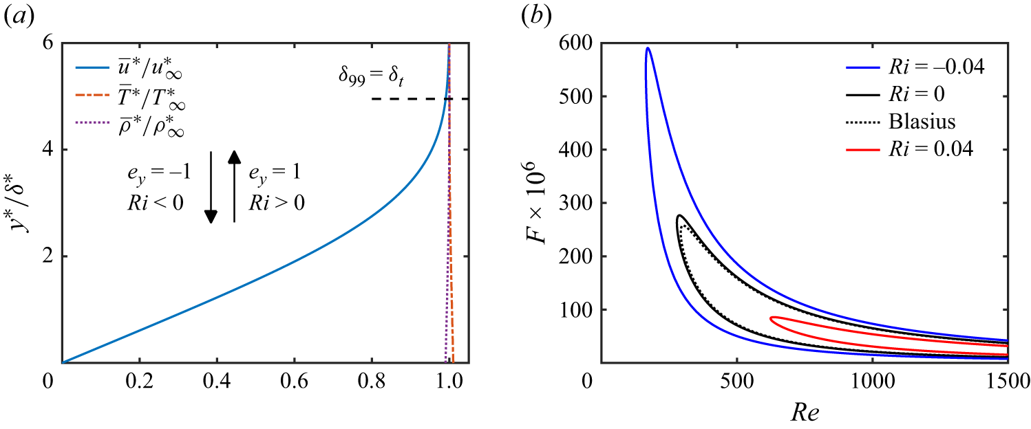


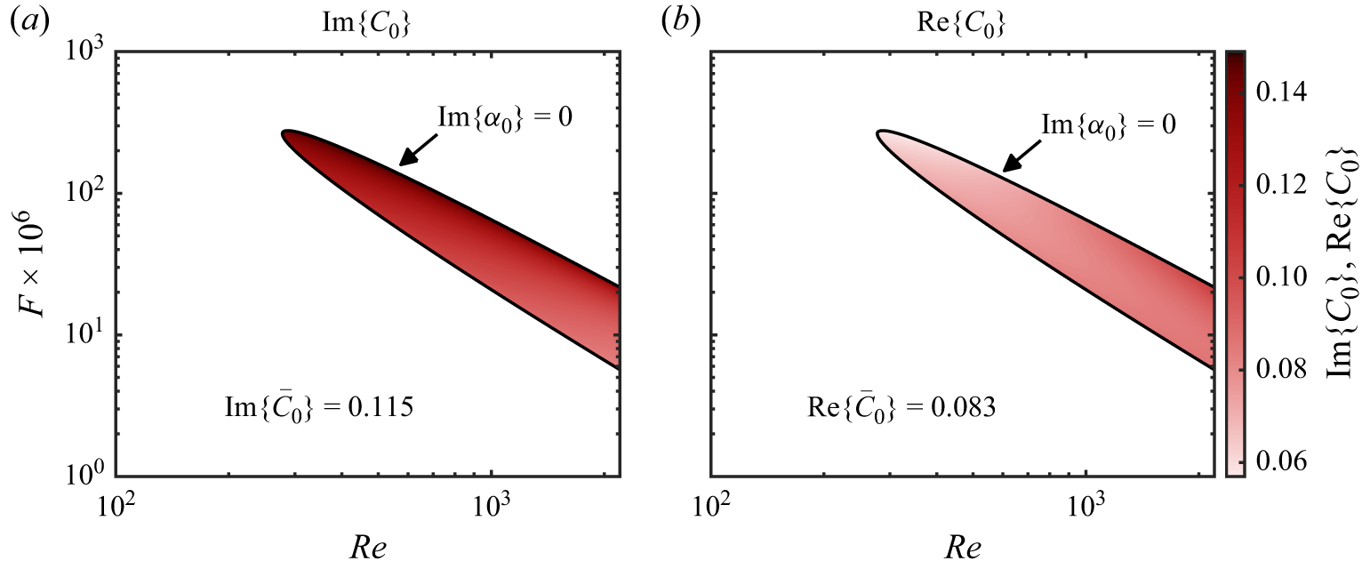


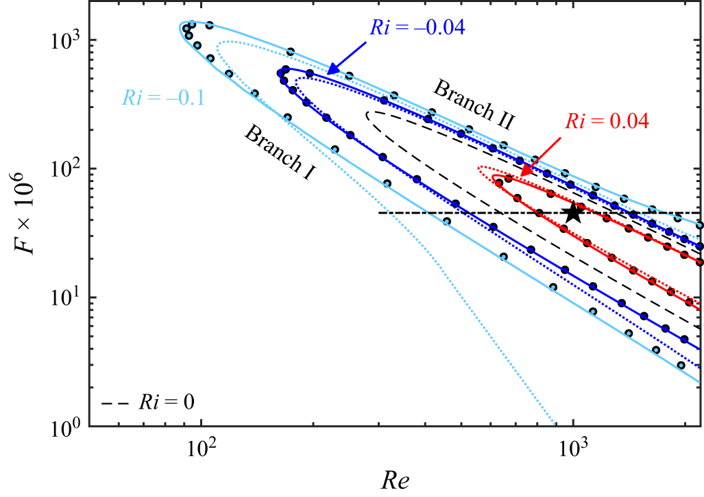


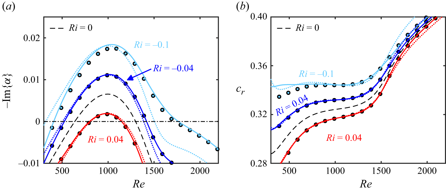


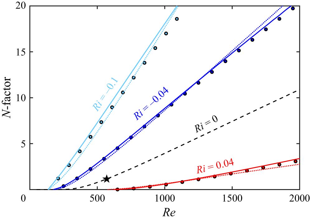


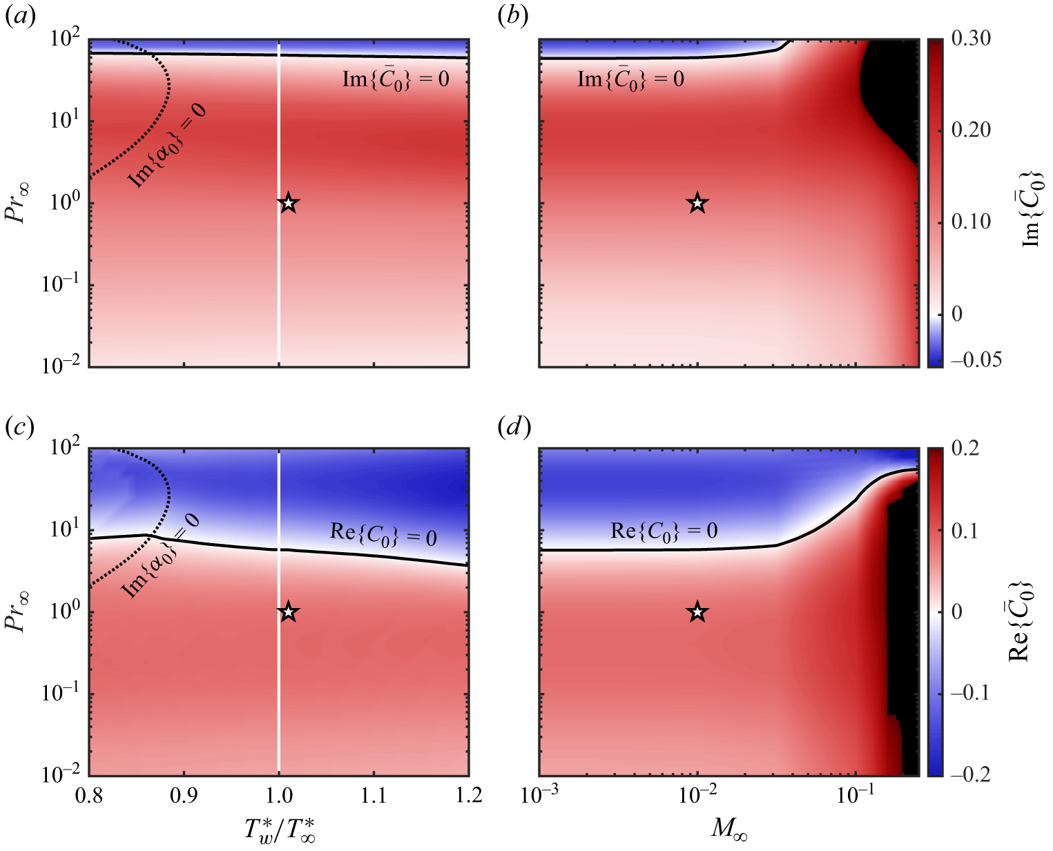


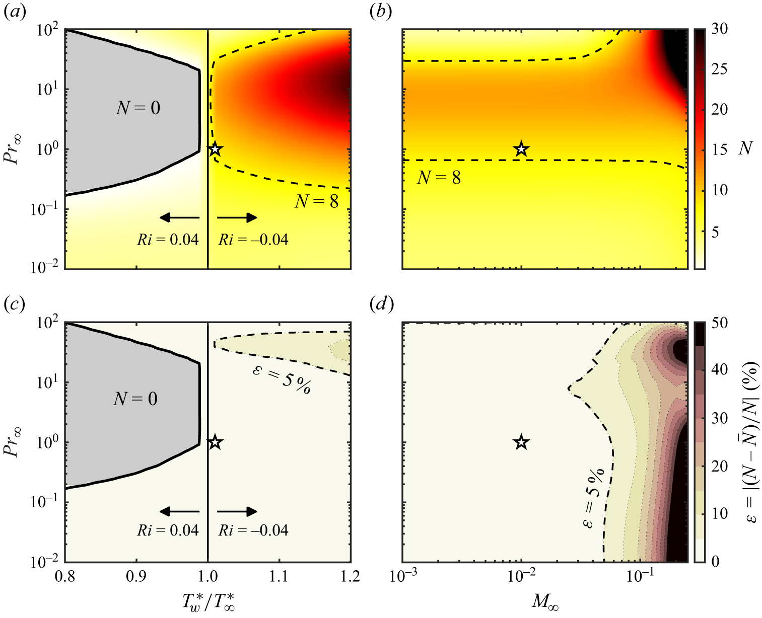


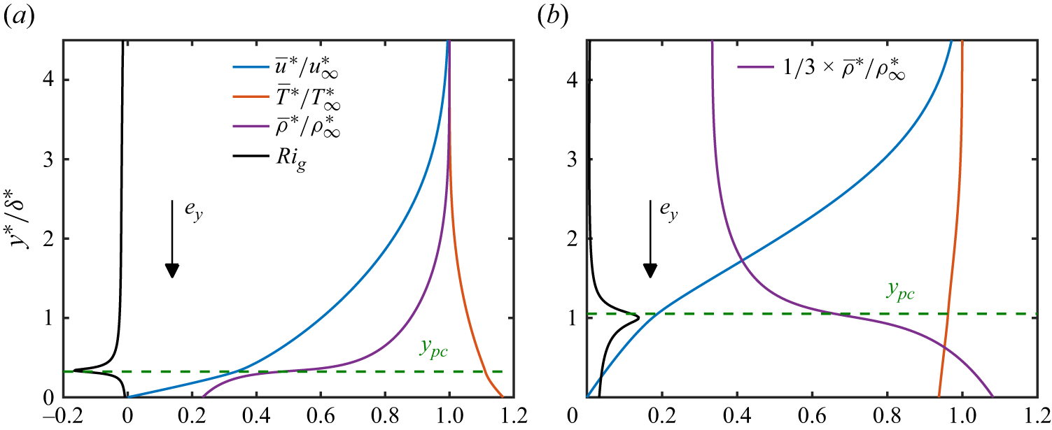


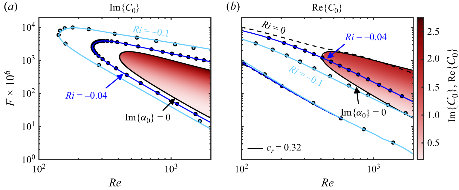


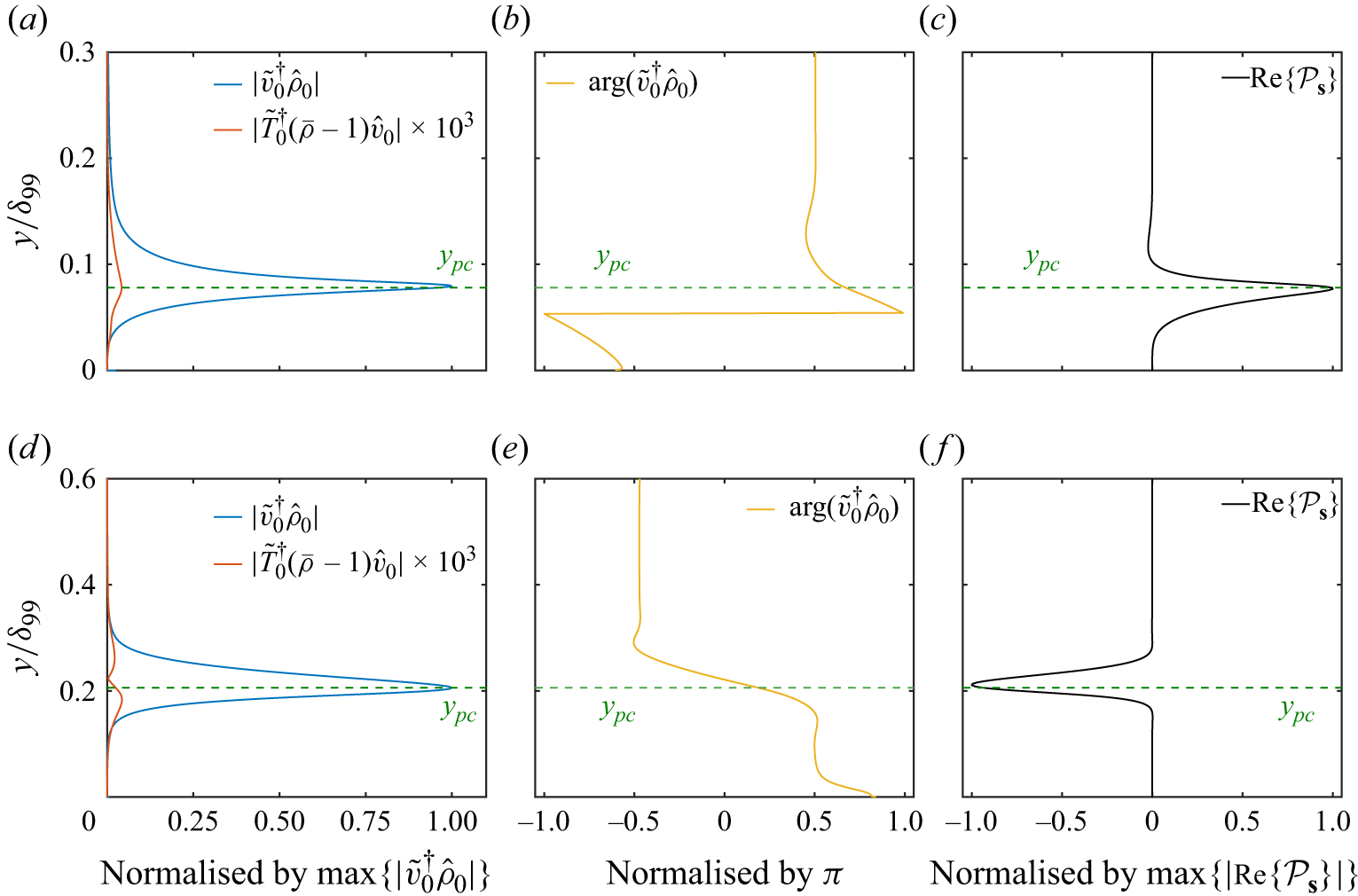


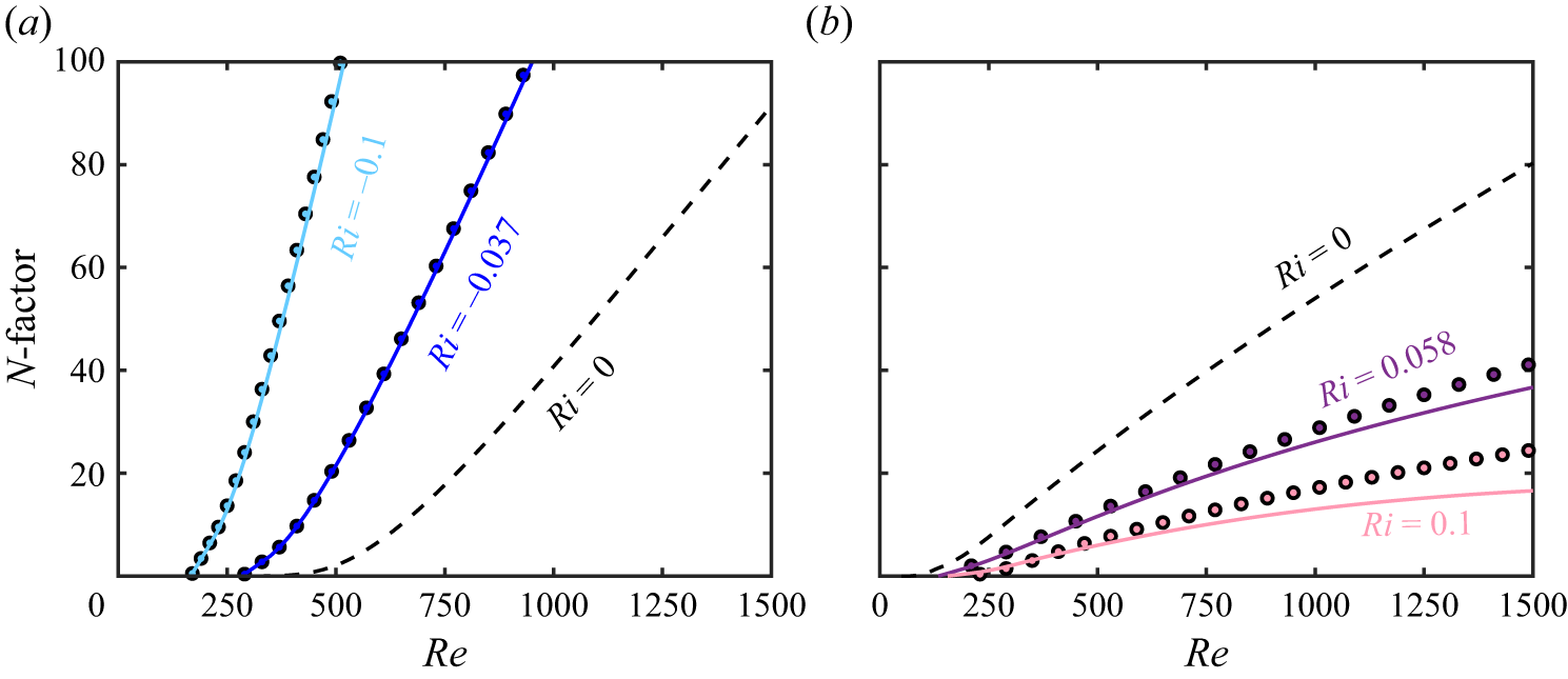


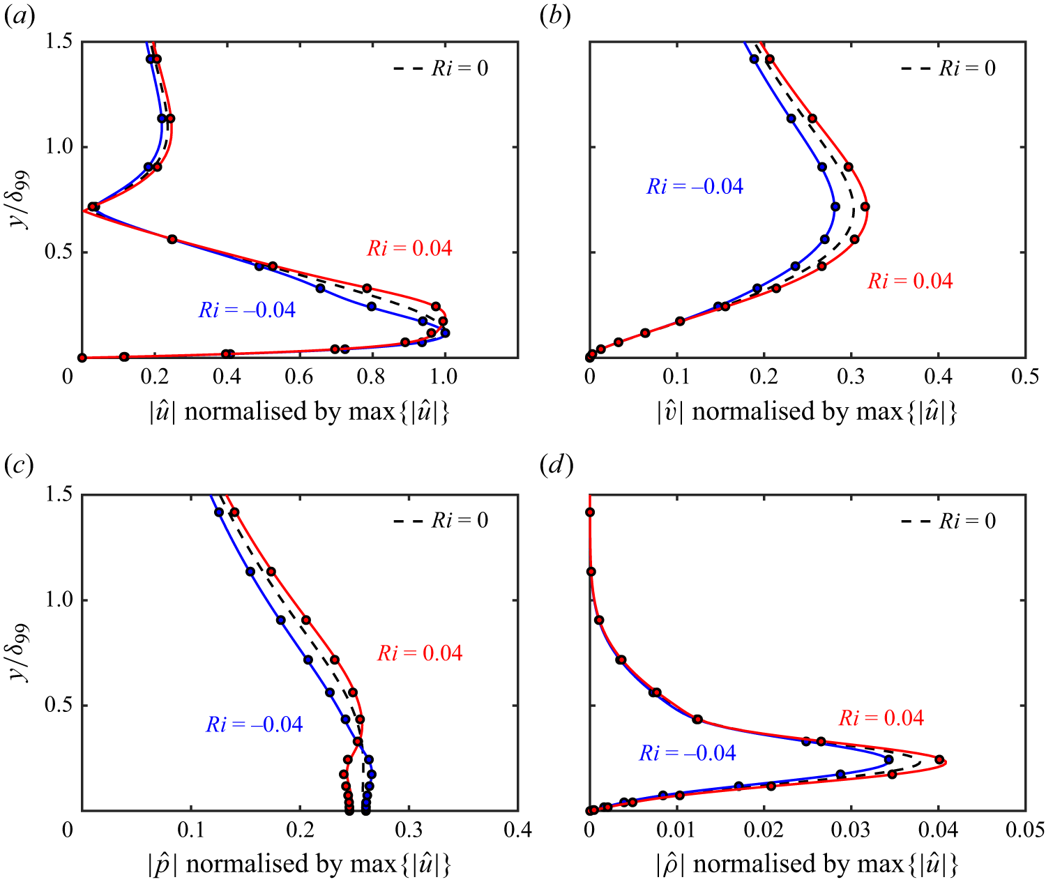


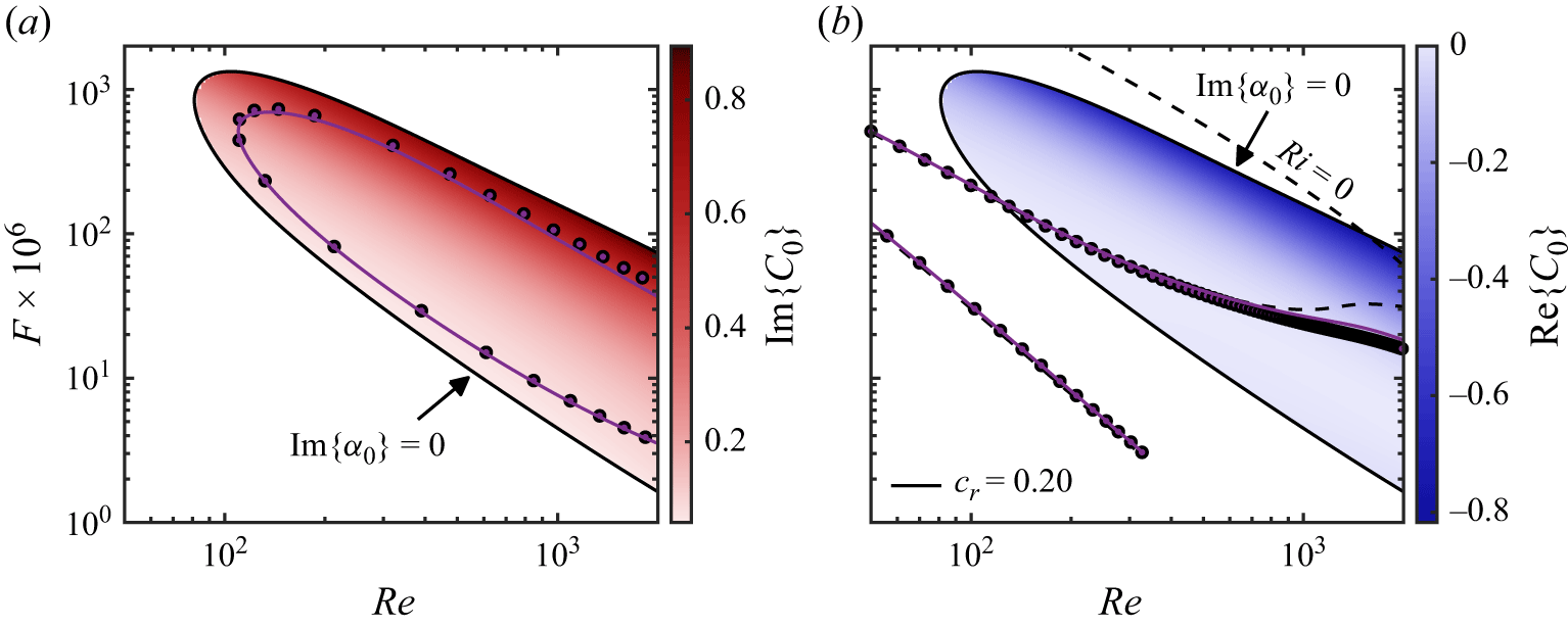


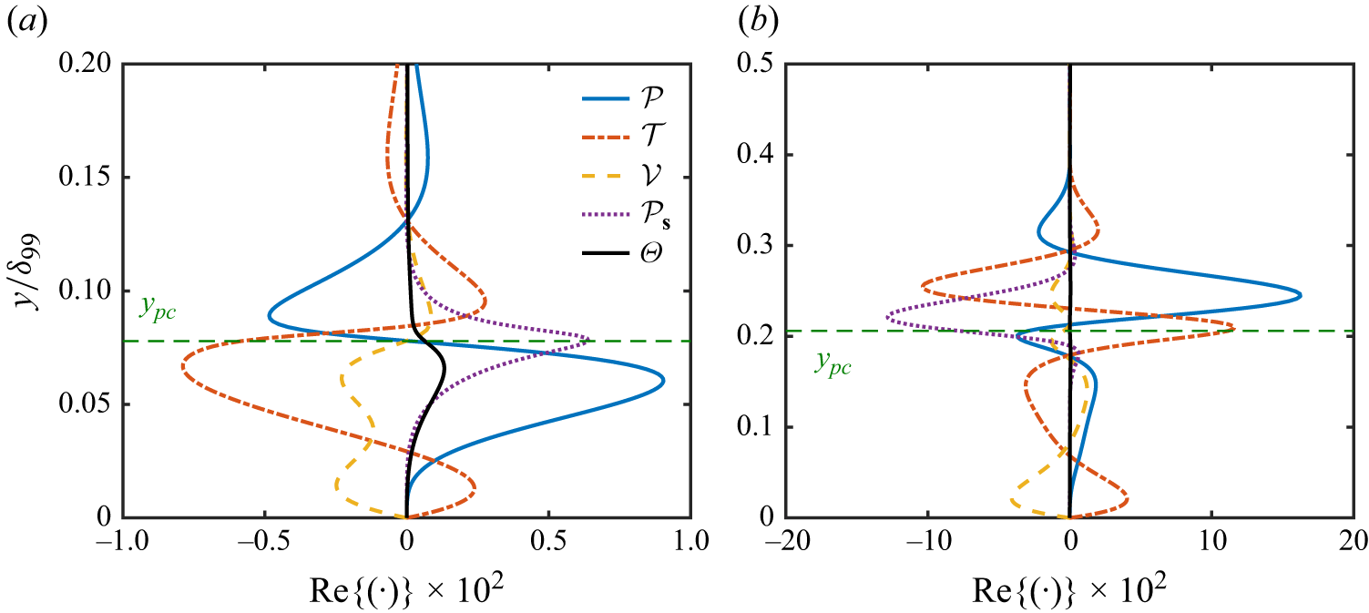


 Open access

