2.1 Elson Lagoon

Elson Lagoon is bounded by the Alaska mainland to the southwest and a chain of barrier islands to the northeast. Sea ice in the lagoon is landlocked (Hata and Tremblay, Reference Hata and Tremblay2015a, Reference Hata and Tremblay2015b; Mahoney, Reference Mahoney, Osborne, Richter-Menge and Jeffries2018) between these boundaries throughout much of the frozen season. The barrier islands protect the landlocked ice from dynamic interactions with passing pack ice and prevent the lagoon ice from breaking away from shore. This protection makes the lagoon a relatively stable platform on which to deploy monitoring equipment for season-long observational campaigns. The Sea ice Dynamics Experiment (SIDEx) team executed such a campaign during the winter of 2018/19 with the aim of measuring thermal stress, strain and fracture in the lagoon ice over the course of a winter season. Measurements of strain from this SIDEx campaign discussed in Section 3.3 are key to this study, providing an independent observation against which to compare modeled displacements.

2.2 Chukchi Sea near Utqiaġvik, Alaska

Our Chukchi Sea study area contains both drifting and landfast ice along a stretch of open coastline offshore from Utqiaġvik, Alaska. Without the protection of barrier islands, landfast ice in this area frequently undergoes dynamic interactions with drifting pack ice. These interactions deform the landfast ice and alter the location of the landfast ice edge several times a season (e.g. Mahoney and others, Reference Mahoney, Eicken and Shapiro2007).

3.1 12 d Sentinel-1 interferograms over Elson Lagoon

The Sentinel 1 (S1) A and B satellite constellation, operated by the European Space Agency, transmits in the C-band with a wavelength of 5.55 cm. Each satellite provides a 12 d repeat pass for creating A–A or B–B interferograms. We used the Alaska Satellite Facility's Hybrid Pluggable Processing Pipeline (HyP3) (Hogenson and others, Reference Hogenson2016) to create fifteen 12 d interferograms over Elson Lagoon from Sentinel 1 image pairs acquired in interferometric wide swath mode between 24 December 2018 and 27 April 2019. Attributes of these images are listed in Supplementary Table S1. HyP3 is a web-based, on-demand platform which performs all interferogram production steps (https://hyp3-docs.asf.alaska.edu/guides/insar_product_guide/), including multi-looking by 10 pixels across-track and 2 pixels along-track to give a final image resolution of 80 m and pixel spacing of 40 m. HyP3 also performs adaptive filtering to improve interferogram coherence, and geocodes each interferogram to automatically assigned UTM zones 4 or 5 with 40 m square pixels. We further smooth each interferogram by taking the moving average of a 5 × 5 pixel window in complex space.

3.2 10 s TanDEM-X interferograms over the Chukchi Sea

Along the Chukchi coast we utilize shorter, 10 s interferograms from the German Aerospace Center's (DLR) Tan-DEM-X (TDX) satellite constellation operated in Stripmap Pursuit Monostatic mode. While the satellites only operated in this mode for a few months in 2010 (Scheiber and others, Reference Scheiber2011), and from October 2014 to March 2015, these 10 s interferograms provide a unique opportunity to use InSAR to quantify surface strain over drifting sea ice.

The TDX satellites operate in the X-band with a wavelength of 3.11 cm. Attributes of the three image pairs used here, acquired between 6 January 2015 and 22 January 2015 are listed in the Supplementary material (Table S2). We follow a similar InSAR processing workflow to that carried out by the HyP3 interface. We co-register each TDX image pair and multi-look each image by 4 pixels across-track and 2 pixels along-track to give an approximate resolution of 10 m. We apply an adaptive filter (Goldstein and Werner, Reference Goldstein and Werner1998) to each interferogram to improve coherence, and georeference each to a zone 4 UTM grid with 5 m square pixels.

3.3 Laser strain observatory measurements of surface displacement in Elson Lagoon

A laser strain observatory (LSO) consisting of a Leica TM-50 total station and array of retro-reflecting prisms provide point displacement measurements on Elson Lagoon throughout the winter 2018/19 SIDEx field campaign. The prisms were mounted on steel posts anchored in the ice at distances of 40–929 m from the central total station and spaced through 360° of azimuth. The total station recorded range, azimuth and zenith to each of 23 retroreflectors at several-minute intervals (dependent on the time taken to locate each reflector in series) from 19 December 2018 to 20 May 2019, with a gap from 23 December 2018 to 16 January 2019 due to a technical issue. The location of the central total station was recorded at the time of deployment using a wide area augmentation system (WAAS) enabled handheld GPS with expected precision of ±3 m. We use this position to locate the LSO array in the UTM projection of each Sentinel 1 interferogram over Elson Lagoon.

The central total station has a manufacturer-stated theoretical accuracy of 1.6 × 10⁻⁶ m (0.6 mm + 1 mm km⁻¹) in range, and 1.4 × 10⁻⁴ degrees in azimuth (2.4 mm at 1 km). Consecutive range measurements during periods of little deformation or atmospheric change show range measurement repeatability approaches 10⁻⁷ m. We correct for range errors caused by variations in air temperature, pressure or humidity using a correction factor calculated from measurements of these parameters collected at an on-site weather station. Calculated correction factors are expected to be accurate to ±1 mm km⁻¹. We therefore expect practical field accuracy in absolute range near 2 × 10⁻⁶ m. We also correct azimuth positions of retroreflectors for gradual drift by subtracting any rotations experienced uniformly by a majority of the reflectors from the azimuth positions of all reflectors.

4.1 Contributions to interferometric phase

A radar signal traveling from a sensor to a scattering surface and back returns to the sensor at some position, called phase, in the radar waveform, recorded as an angle between −π and π radians. InSAR analysis evaluates pixel-by-pixel differences in returned phase between two coherent and aligned SAR images to create an interferogram (Moreira and others, Reference Moreira2013). These phase differences, called interferometric phase, ϕ, are caused by real or apparent changes in line-of-sight signal path length from the sensor to the surface, Δr, between images:

(1)$$\phi = \displaystyle{{4\pi \;( {{\rm \Delta }r\% ( \lambda /2) } ) } \over \lambda }$$

Like the returned phase in each interfered image, ϕ is a circular value, wrapping over an interval of 2π radians. If Δr is smoothly varying and differences between neighboring pixels are small (≪ λ/2), ϕ creates patterns of phase wraps called fringes across an interferogram. Over such areas, phase can be unwrapped to remove the 2π ambiguity in Eqn (1), allowing evaluation of relative differences in Δr between pixels.

Observed ϕ across an interferogram is the sum of several components arising from different processes that alter the real or apparent range, r, from the sensor to the surface:

(2)$$\phi = \phi _{{\rm def}} + \phi _{{\rm topo}} + \phi _{{\rm atm\;}} + \phi _\gamma $$

where ϕ _def is the contribution from surface deformation, or strain; ϕ _topo is the contribution from topographic relief; ϕ _atm is the contribution from changing atmospheric conditions and $\phi _\gamma$ is the contribution from decorrelation.

4.2 Excluding non-deformation components of phase

In this work, we assume ϕ _def is the primary component of total observed ϕ.

ϕ _topo arises from changes in satellite position and varies proportionally to topographic height, h _topo, and the perpendicular baseline distance, B _⊥, between sensor locations during each acquisition:

(3)$$\phi _{{\rm topo}} = h_{{\rm topo}}\displaystyle{{4\pi B_\bot } \over {\lambda r\cos ( \theta ) }}\;$$

In a sea-ice environment, pressure ridges represent the largest topographic variation. The 95th percentile of pressure ridge sail heights across the Arctic is 2 m and modal width is 35 m (Duncan and Farrell, Reference Duncan and Farrell2022). For typical B _⊥ on the order of 10² m and slant range, r, on the order of 900 km, such ridges will cause a similar phase response to millimeter-scale line-of-sight displacements. Moreover, since ridges are only one or a few pixels wide, their phase signature cannot be extensively monotonic. We can therefore assume ϕ _topo is negligible where phase gradients are sustained and monotonic over distances greater than tens of meters.

Changes in atmospheric conditions between two acquisitions cause apparent range changes by altering the signal's speed or path curvature, giving rise to an atmospheric component, ϕ _atm. We expect contributions from ϕ _atm to be small in comparison to other components following Dammann and others (Reference Dammann, Eicken, Meyer and Mahoney2016). Both study sites are in areas with minimal topographic relief (Jolivet and others, Reference Jolivet, Grandin, Lasserre, Doin and Peltzer2011, Reference Jolivet2014) and ϕ _atm tends to be largest in areas of mountainous terrain. Additionally, the 10 s interval of TDX interferograms provides little time for significant atmospheric change. We therefore do not consider ϕ _atm further.

Finally, thermal instrument noise, temporal and spatial decorrelation, and changes in surface scattering properties between acquisitions contribute to apparent changes in range, leading to a decorrelation component, $\phi _\gamma$. The expected variance of the decorrelation component $\phi _\gamma$ increases with decreasing coherence, γ (Rosen and others, Reference Rosen2000). γ is a metric of interferometric phase quality, which takes on values between 0, indicating no correlation between primary and secondary interfered images, and 1, indicating that the primary and secondary images contain exactly the same phase (Woodhouse, Reference Woodhouse2006). We limit the magnitude of $\phi _\gamma$ by limiting our analysis to regions of continuous phase in which more than 75% of pixels maintain complex coherence, γ, >0.35.

4.3 Identification and exclusion of vertically dominated displacement

The line-of-sight component of surface motion may be composed of horizontal displacement, d _h, and vertical displacement, d _v, whose contributions to ϕ _def depend on the elevation angle, θ, between each pixel and the satellite:

(4)$$\phi _{{\rm def}} = \displaystyle{{4\pi } \over \lambda }( d_{\rm h}\cos \theta + d_{\rm v}\sin \theta ) $$

Our aim here is to interpret horizontal displacements alone. However, typical SAR elevation angles provide similar sensitivity to both d _h and d _v, and gradients in d _h and d _v can have similar magnitudes. This means vertical and horizontal displacements can make similar contributions to ϕ _def that are difficult to separate. We therefore need to exclude interferograms containing significant vertical displacements. We do this by limiting our analysis to interferograms or regions of interferograms in which the gradient in ϕ is monotonic along the look direction of the satellite, following Dammann and others (Reference Dammann, Eicken, Meyer and Mahoney2016). This criterion for assuming d _v is negligible follows from the observation that gradients in d _v, or surface tilts, cannot continue indefinitely. Whether arising from sea surface tilt, thermodynamic or dynamic buckling, or wave activity, gradients in d _v exhibit undulations at length scales of hundreds of m to tens of kilometers (Evans and others, Reference Evans, Untersteiner, Evans and Untersteiner1971; Kwok and Morison, Reference Kwok and Morison2016; Mahoney and others, Reference Mahoney, Dammann, Johnson, Eicken and Meyer2016). Strains are not similarly spatially limited. Therefore, if a phase gradient is monotonic over tens of kilometers, vertical displacements must be negligible. If the phase gradient exhibits small undulations that do not overwhelm a stronger monotonic gradient, undulations may be filtered out and vertical deformation assumed negligible in the remaining signal. We apply such filtering to TDX interferograms. If the phase gradient exhibits strong undulations relative to the overall phase gradient, such filtering cannot be applied and horizontal and vertical contributions are inseparable without additional information. This is the case in some regions of Elson Lagoon, which we remove from analysis. Wang and others (Reference Wang2020) as well as Chen and others (Reference Chen2021) do present alternative quantitative methods for separating vertical and horizontal sea-ice displacement components using multi-orbit InSAR techniques. However, their methods require the assumption that deformation occurs at a constant rate over the multi-day interval spanned by overlapping InSAR pairs from ascending and descending orbits. The episodic nature of processes causing sea surface tilt and sea-ice deformation means this condition is rarely met and so we do not adopt this approach here.

5.1 RSVP identification

Unwrapping, or spatially integrating, phase values across continuous RSVPs simplifies inverse model calculations by removing relative 2π phase ambiguity. Within an RSVP, or area of sequential, continuous fringes bounded by discontinuities, differences in unwrapped phase between pixels are directly proportional to the line-of-sight component of relative displacement between them. Relative displacement between pixels located in separate RSVPs cannot be evaluated, since an unknown number of phase wraps are lost at RSVP boundaries. We identify RSVPs in each interferogram to allow accurate unwrapping and to delineate where we can or cannot evaluate relative displacements in later steps. Dulam and others (Reference Dulam, Fedders, Mahoney and Kambhamettu2023) describe recent advancement toward automated RSVP boundary detection in ground-based radar interferograms over sea ice, but similar methods are not operational for satellite-acquired interferograms. Instead, we use the hybrid automated and manual approach described below.

Discontinuities at RSVP boundaries generally appear as an abrupt change in the magnitude or orientation of the phase gradient. To detect these abrupt changes, we first calculate phase gradient components ∂ϕ/∂x and ∂ϕ/∂y in complex space using Eqns (5) and (6), following Libert and others (Reference Libert, Wuite and Nagler2022). These equations yield an average phase slope over a w × w window of pixels, where w must be odd and >1. We set w = 3 for maximum gradient resolution and assign the calculated average slope to the center pixel in each window. Calculating the gradient in complex space ensures correct slope magnitude where phase wraps between −π and π radians:

(5)$$\left. {\displaystyle{{\partial \phi } \over {\partial x}}} \right\vert _{( {x_k, y_l} ) } = {\rm atan}2\left({\mathop \sum \limits_{m = k-( w-1) /2}^{k + ( w-1) /2} \mathop \sum \limits_{n = l-( w-1) /2}^{l + ( w-1) /2} {\rm e}^{i( {\phi_{m + 1, n-\phi_{m, n}}} ) }} \right)$$

(6)$$\left. {\displaystyle{{\partial \phi } \over {\partial y}}} \right\vert _{( {x_k, y_l} ) } = {\rm atan}2\left({\mathop \sum \limits_{m = k-( w-1) /2}^{k + ( w-1) /2} \mathop \sum \limits_{n = l-( w-1) /2}^{l + ( w-1) /2} {\rm e}^{i( {\phi_{m, n + 1-\phi_{m, n}}} ) }} \right)$$

We convert ∂ϕ/∂x and ∂ϕ/∂y into slope magnitude, s, and fringe azimuth, α _f, pairs using Eqns (7) and (8), respectively. α _f records the direction of the most positive phase slope, perpendicular to lines of fringes in an interferogram, as an angle counter-clockwise from east:

(7)$$s = \sqrt {{\displaystyle{{\partial \phi } \over {\partial y}}}^2 + {\displaystyle{{\partial \phi } \over {\partial x}}}^2} $$

(8)$$\alpha _{\rm f} = {\rm atan}2\left({\displaystyle{{\partial \phi } \over {\partial y}}, \;\displaystyle{{\partial \phi } \over {\partial x}}} \right)$$

We identify discontinuities where the std dev. of the phase slope over a 5 × 5 pixel moving window exceeds a threshold of 3.16 × 10⁻³ rad m⁻¹. This threshold was chosen as the mean 95th percentile of slope std devs. over coherent (γ > 0.35) pixels in Elson Lagoon. This threshold is likely not universally generalizable, but worked here to identify most discontinuities without identifying false boundaries due to isolated areas of low coherence. We manually connect detected discontinuities arranged in linear patterns and add any additional obvious discontinuities which were not detected by thresholding. This manual step is important for identifying boundaries between regions where fringe patterns to either side show slopes of similar magnitude, and perhaps even orientation, but are clearly offset from one another. Land pixels in both study areas and pixels beyond the barrier islands in the Elson Lagoon study area are removed using a hand-drawn mask.

5.2 Phase unwrapping within RSVPs in Sentinel 1 interferograms

For Sentinel 1 interferograms, once RSVPs are delineated as described above, we unwrap each RSVP individually using a three-step process. We first integrate phase at pixels with coherence >0.2 using the branch cut unwrapping algorithm provided in the GAMMA software package (Werner and others, Reference Werner, Wegmüller and Strozzi2002). We use adaptive-window interpolation to fill gaps in unwrapped phase where low coherence pixels were skipped. Then we use the unwrapped, filled interferograms as a model for unwrapping the low-coherence pixels using the same branch-cut algorithm as in step 1. We adjust unwrapped phase in each RSVP to have a mean value of zero to obtain appropriate relative displacement magnitudes between points in later steps.

5.3 Phase unwrapping within RSVPs in TDX interferograms

For TDX interferograms, we begin by following the same unwrapping method as for Sentinel 1 interferograms. Then we fit a planar surface to each unwrapped RSVP and use this smoothed, planar unwrapped phase for all further analysis. This smoothing step preserves the majority of the phase gradient, which we attribute to horizontal motion, while removing the periodic signals Mahoney and others (Reference Mahoney, Dammann, Johnson, Eicken and Meyer2016) show to arise from vertical displacement due to infragravity waves (Fig. 2). A few isolated, non-periodic residual signals found at asperities along RSVP boundaries (e.g. white arrows in Fig. 2), likely indicating elevated strain at these point contact locations, are also lost in the smoothing process. However, these residual signals are spatially confined and contain less than one full phase wrap each, and overall correlation coefficients between original unwrapped phase and fitted, smooth unwrapped phase are ⩾0.8 in 88% of RSVPs.

Figure 2.

TDX interferogram from 6 January 2015 (a) original, wrapped, (b) unwrapped with waves removed, re-wrapped for ease of visual comparison. (c) The residual signal left behind by the unwrapping and smoothing process (panel a minus panel b) contains low amplitude wave signals.

6.1 Model concept: geometric relationships between displacement and ϕ

Any sea-ice deformation or displacement in the horizontal plane may be fully described by some combination of five modes: uniaxial convergence, simple shear, isotropic radial convergence, rigid rotation and rigid translation. Divergence is represented as a negative convergence. The fringe pattern in a monotonic interferogram therefore records the sum of one or more component phase gradients associated with each of these horizontal deformation modes:

(9)$$\phi _{{\rm def}} = \phi _{{\rm ax}} + \phi _{{\rm shear}} + \phi _{{\rm rad}} + \phi _{{\rm rot}} + \phi _{{\rm trans}}$$

Each horizontal mode on its own creates phase gradients whose slope, s, and orientation, α _f, exhibit defined geometric relationships with satellite look direction, α _l, deformation magnitude and deformation orientation. Radially symmetric deformation modes produce phase gradients with orientations that depend only on the look direction. Radial convergence leads to phase gradients with α _f parallel to the look direction such that α _f = α _l or α _f =  α _l + π (Figs 3a, b), while rotation creates phase gradients perpendicular to the look direction such that α _f = α _l ± π/2 (Figs 3c, d). For these modes, the magnitude of the phase gradient depends directly on the magnitude of the deformation. In contrast, axially symmetric deformation modes (uniaxial convergence and simple shear) produce interferometric phase gradients whose orientation varies with deformation direction and is less strictly tied to α _l (Figs 3e–t). The magnitude of the phase gradient for these axial modes depends on both the magnitude of deformation and the degree of alignment between α _l and the direction of surface displacement.

Figure 3.

Interferometric fringe patterns associated with positive (a) and negative (b) radial convergence, clockwise (c) and counter-clockwise (d) rotations, and with varying orientations of positive (e–h) and negative (i–l) axial convergence, right-lateral (m–p) and left-lateral (q–t) simple shear, and rigid translation (u–x). White arrows show the direction of surface displacements. Black and red arrows mark the look direction, α _l, and phase gradient azimuth, α _f. For each mode, all displacement fields represent the same strain magnitude.

Translation can only produce phase gradients with α _f parallel to the orientation of the gradient in elevation angle across the image, $\alpha _\theta$, which is nearly parallel to α _l. The magnitude of the phase gradient produced by translation depends strongly not only on the magnitude of the component of displacement parallel to $\alpha _\theta$, but also on the magnitude of the elevation angle gradient across an image (Figs 3u–x). This across-track gradient in θ also makes a small contribution to phase gradients arising from the radial and axial modes discussed above. However, in those cases where there is a gradient in look parallel displacement, the effect of the gradient in θ across the swath is a second-order effect. We use these geometric relationships between deformation characteristics and interferogram characteristics to derive a separate set of analytical inverse equations for each horizontal deformation mode.

However, we also note the ambiguity inherent in inverting 2-D displacements from the 1-D information contained in the interferometric phase gradient. A near-infinite set of 2-D, horizontal displacement fields exists that would reproduce the interferometric pattern in any RSVP exactly. A few examples of this ambiguity are illustrated in Figure 4. For any RSVP, axial convergence and simple shear displacement solutions exist that would reproduce the observed phase gradient exactly, regardless of the mode or modes that contributed to real surface displacement. Similarly, radial convergence, translation and rotation solutions exist that would reproduce the entire look-parallel or look-perpendicular component of the phase gradient, regardless of whether any of these modes contributed at all to the real displacement field. Ambiguity between displacement solutions multiplies when the realistic possibility of combined deformation modes is considered.

Figure 4.

Same fringe pattern obtained from the same α _l (black arrow) can be produced by a myriad of different surface displacement fields (white arrows), that all share the same line-of-sight displacement component.

To achieve a unique modeled displacement field that correctly describes a real displacement field, the real displacement field must be a simple one. By this we mean that either (1) a single deformation mode is responsible for the majority of surface displacement and contributions from other modes can be assumed to be negligible, or (2) the displacement field can be approximated by no more than two deformation modes, and the observed phase gradient is uniform, such that each contributing mode may be described by a single orientation and magnitude pair. If fringes are curved or the phase gradient is variable, not only the orientation or magnitude of either mode, but also how or whether it varies across the RSVP would need to be constrained. This would be intractable without extensive field measurements.

In the single mode case, we can conduct analytical inversion using equations in Sections 6.2–6.4 directly on the unwrapped phase in each RSVP. In a two-mode case, we first split the unwrapped phase in each RSVP into two components corresponding with the contributions of each mode following Eqn (10). $\widehat{{\alpha _{\rm f}}}, \;\widehat{{\;\alpha _{{\rm f}1}}}, \;\;\;\widehat{{\alpha _{{\rm f}2}}}$ are unit vectors pointing in the phase gradient direction and the phase gradient directions associated with the two component displacement modes. s, s ₁, s ₂ are the magnitudes of the phase gradient and the magnitudes of the phase gradients associated with each component mode:

(10)$$\hat{\alpha }_{\rm f}s = \left[{\matrix{ {{\hat{\alpha }}_{{\rm f}1}} & {{\hat{\alpha }}_{{\rm f}2}} \cr } } \right]\left[{\matrix{ {s_1} \cr {s_2} \cr } } \right]$$

We then invert displacement fields associated with each component of the phase gradient individually and sum them to obtain the total, two-mode modeled displacement field.

In this work, as outlined in Sections 6.6 and 6.7, we use a combination of environmental context and elimination of modes or mode combinations requiring clearly non-physical model results to constrain model ambiguity. While our reasoning is site specific, the examples described here provide a framework to guide successful application of this method at other sites also.

6.2 Analytical inverse method for radially symmetric modes

Since radially symmetric modes can only produce phase gradients parallel or perpendicular to α _l, we begin by calculating the look-parallel ($\alpha _\parallel )$ and look-perpendicular (α _⊥) components of the phase slope across each RSVP according to Eqns (11)–(12), where α _diff is the interior angle between α _l and α _f:

(11)$$\displaystyle{{\partial \phi } \over {\partial \alpha _\parallel }} = s\,{\rm cos}( {\alpha_{{\rm diff}}} ) $$

(12)$$\displaystyle{{\partial \phi } \over {\partial \alpha _\bot }} = s\,\sin \alpha _{{\rm diff}}$$

We take the average of each slope component, $\overline {\partial \phi } /\partial \alpha _\parallel$, and $\overline {\partial \phi } /\partial \alpha _\bot$, across each RSVP to account for isotropic radial convergence and rigid rotation.

Displacement magnitude in these radially symmetric modes scales with distance from a center of deformation. We cannot define this center in an absolute reference frame due to the 2π ambiguity in observed ϕ, but the center of relative deformation may be chosen arbitrarily with no impact on modeled strain. We assign the centroid of each RSVP as the center of relative deformation for simplicity.

For each RSVP, we calculate the distance, d, from the centroid to each pixel. The magnitude of relative radial, Δd _rad, or rotational, Δd _rot, displacement at each pixel is then calculated according to Eqn (13) or (14) where θ is the elevation angle from the satellite to a pixel:

(13)$${\rm \Delta }d_{{\rm rad}} = \overline {\displaystyle{{\partial \phi } \over {\partial \alpha _\parallel }}} d\displaystyle{{-\lambda } \over {4\pi \cos ( \theta ) }}$$

(14)$${\rm \Delta }d_{{\rm rot}} = \overline {\displaystyle{{\partial \phi } \over {\partial \alpha _\bot }}} \;d\;\displaystyle{{-\lambda } \over {4\pi \cos \theta }}$$

The displacement Δd _rad is positive in the direction pointing from the RSVP centroid to the center of each RSVP pixel, α _rad. We convert Δd _rad to easting and northing displacements u _rad, v _rad via Eqns (15) and (16), below:

(15)$$u_{{\rm rad}} = {\rm \Delta }d_{{\rm rad}}\cos \alpha _{{\rm rad}}$$

(16)$$v_{{\rm rad}} = {\rm \Delta }d_{{\rm rad}}\sin \alpha _{{\rm rad}}$$

Δd _rot is perpendicular to α _rad, either in a clockwise direction, indicated by $( {\widehat{{\alpha_{\rm f}}} \times \widehat{{\alpha_{\rm l}}}} ) < 0$, or counter-clockwise direction, indicated by $( {\widehat{{\alpha_{\rm f}}} \times \widehat{{\alpha_{\rm l}}}} ) > 0$, where $\widehat{{\alpha _{\rm f}}}$ and $\widehat{{\alpha _{\rm l}}}$ are unit vectors pointing in the α _f and α _l directions, respectively. Thus, the easting and northing components of rotation u _rot, v _rot are calculated via Eqns (17) and (18).

(17)$$u_{{\rm rot}} = \left\{{\matrix{ {{\rm \Delta }d_{{\rm rot}}{\rm sin}( {\alpha_{{\rm rot}}} ) } & {( {\widehat{{\alpha_{\rm f}}} \times \widehat{{\alpha_{\rm l}}}} ) < 0} \cr {-{\rm \Delta }d_{{\rm rot}}{\rm sin}( {\alpha_{{\rm rot}}} ) } & {( {\widehat{{\alpha_{\rm f}}} \times \widehat{{\alpha_{\rm l}}}} ) > 0} \cr } } \right.\;$$

(18)$$v_{{\rm rot}} = \left\{{\matrix{ {-{\rm \Delta }d_{{\rm rot}}{\rm cos}( {\alpha_{{\rm rot}}} ) } & {( {\widehat{{\alpha_{\rm f}}} \times \widehat{{\alpha_{\rm l}}}} ) < 0} \cr {{\rm \Delta }d_{{\rm rot}}{\rm cos}( {\alpha_{{\rm rot}}} ) } & {( {\widehat{{\alpha_{\rm f}}} \times \widehat{{\alpha_{\rm l}}}} ) > 0} \cr } } \right.$$

6.3 Analytical inverse method for axially symmetric modes

For axially symmetric modes, we begin by calculating the horizontal projection, Δr _hz, of recorded line-of-sight displacement using Eqn (19):

(19)$${\rm \Delta }r_{{\rm hz}} = \displaystyle{{-\lambda \phi _{unw}} \over {4\pi }}\displaystyle{1 \over {\cos \theta }}$$

For these modes, displacement magnitude scales with distance from an axis of deformation rather than a single central point. We again cannot determine the absolute location of deformation axes but choose the line ϕ _unw = 0 in each RSVP as the axis of relative deformation for simplicity. We calculate the magnitudes of horizontal displacement for axial divergence, Δd _ax, or simple shear, Δd _sh, that yield Δr _hz when projected onto the look direction as Eqns (20) and (21) below:

(20)$$\;{\rm \Delta }d_{{\rm ax}} = \displaystyle{{{\rm \Delta }r_{{\rm hz}}} \over {\cos \alpha _{{\rm diff}}}}\;$$

(21)$${\rm \Delta }d_{{\rm sh}} = \displaystyle{{{\rm \Delta }r_{{\rm hz}}} \over {\sin \alpha _{{\rm diff}}}}$$

Axial divergence gives rise to fringes with α _f parallel to the direction of displacement, so we calculate the easting and northing components u _ax, v _ax as (22) and (23).

(22)$$u_{{\rm ax}} = {\rm \Delta }d_{{\rm ax}}\cos \alpha _{\rm f}$$

(23)$$v_{{\rm ax}} = \Delta d_{{\rm ax}}\sin \alpha _{\rm f}$$

Shear deformation produces fringes with α _f perpendicular to the direction of motion, with $( {\widehat{{\alpha_{\rm f}}} \times \widehat{{\alpha_{\rm l}}}} ) < 0$ indicating right lateral simple shear, and $( {\widehat{{\alpha_{\rm f}}} \times \widehat{{\alpha_{\rm l}}}} ) > 0$ indicating left lateral simple shear. Easting and northing components, u _sh, v _sh are calculated as Eqns (24) and (25).

(24)$$u_{{\rm sh}} = \left\{{\matrix{ {{\rm \Delta }d_{{\rm sh}}\sin ( {\alpha_{\rm f}} ) } & {( {\widehat{{\alpha_{\rm f}}} \times \widehat{{\alpha_{\rm l}}}} ) < 0} \cr {-{\rm \Delta }d_{{\rm sh}}{\rm sin}( {\alpha_{\rm f}} ) } & {( {\widehat{{\alpha_{\rm f}}} \times \widehat{{\alpha_{\rm l}}}} ) > 0} \cr } } \right.$$

(25)$$v_{{\rm sh}} = \left\{{\matrix{ {-{\rm \Delta }d_{{\rm sh}}\cos ( {\alpha_{\rm f}} ) } & {( {\widehat{{\alpha_{\rm f}}} \times \widehat{{\alpha_{\rm l}}}} ) < 0} \cr {{\rm \Delta }d_{{\rm sh}}{\rm cos}( {\alpha_{\rm f}} ) } & {( {\widehat{{\alpha_{\rm f}}} \times \widehat{{\alpha_{\rm l}}}} ) > 0} \cr } } \right.$$

6.4 Analytical inverse method for translation

To model rigid translations, we begin by calculating the slope, $s_\theta$, and azimuth, $\alpha _\theta$ of the spatial gradient in elevation angle across the interferogram, as well as the component of phase slope parallel to this gradient $\partial \phi /\partial \alpha _\theta$. We differentiate Eqn (4), in an arbitrary, horizontal dimension, h, continuing our assumption of no vertical displacement to obtain Eqn (26).

(26)$$\displaystyle{{\partial \phi } \over {\partial h}} = \displaystyle{{4\pi } \over \lambda }\left({\displaystyle{{\partial d_{\rm h}} \over {\partial h}}{\rm cos}\theta -d_{\rm h}\sin \theta \displaystyle{{\partial \theta } \over {\partial h}}} \right)$$

In the absence of strain, d _h contains only rigid translation, d _tran, and (26) simplifies to (27)

(27)$$\displaystyle{{\partial \phi } \over {\partial h}} = \displaystyle{{4\pi } \over \lambda }\left({-d_{{\rm tran}}\displaystyle{{\partial \theta } \over {\partial h}}\sin \theta } \right)$$

If we choose h to be the direction of the gradient in elevation angle, Eqn (27) may be rearranged to solve for translation, giving (28):

(28)$$d_{{\rm tran}} = \displaystyle{{-\lambda ( \partial \phi /\partial \alpha _\theta ) } \over {4\pi ( {s_\theta \sin \theta } ) }}$$

If the assumption that the phase gradient contains no strain is incorrect (i.e. displacement is not uniform across an RSVP), this method will overestimate translation magnitudes due to the additional component of $\partial \phi /\partial \alpha _\theta$ contributed by any gradient in surface displacement. To minimize this overestimation, we take the median value of d _tran to be the best estimate of translation across each RSVP. This median displacement is then divided into easting and northing components u _tran and v _tran according to Eqns (29) and (30):

(29)$$u_{{\rm tran}} = -d_{{\rm tran}}\cos \alpha _\theta $$

(30)$$v_{{\rm tran}} = d_{{\rm tran}}\sin \alpha _\theta $$

6.5 Strain calculation from modeled horizontal displacements

From each modeled displacement field, we can derive first and second principal components of strain, $\varepsilon _1$ and $\varepsilon _2$. Normal strains on planes parallel to the x (easting) and y (northing) directions $\varepsilon _{xx}$ and $\varepsilon _{yy}$ and shear strain on these planes τ _xy are calculated according to Eqns (31)–(33). τ _xy may include both pure and simple shear components, depending upon the orientation of the strain field:

(31)$$\varepsilon _{xx} = \displaystyle{{{\rm \Delta }u} \over {{\rm \Delta }x}}$$

(32)$$\varepsilon _{yy} = \displaystyle{{{\rm \Delta }v} \over {{\rm \Delta y}}}$$

(33)$$\tau _{xy} = \displaystyle{1 \over 2}\left({\displaystyle{{{\rm \Delta }u} \over {{\rm \Delta }y}} + \displaystyle{{{\rm \Delta }v} \over {{\rm \Delta }x}}} \right)$$

We can then calculate the angle of first principal strain according to Eqn (34),

(34)$$\theta _p = {\rm atan}\left({\displaystyle{{2\tau_{xy}} \over {\varepsilon_{xx}-\varepsilon_{yy}}}} \right)\displaystyle{1 \over 2}$$

and calculate $\varepsilon _1$ and $\varepsilon _2$ as Eqn (35):

(35)$$\left[{\matrix{ {\varepsilon_1} & 0 \cr 0 & {\varepsilon_2} \cr } } \right] = \left[{\matrix{ {\cos ( {\theta_p} ) } & {\sin ( {\theta_p} ) } \cr {- \!\sin ( {\theta_p} ) } & {\cos ( {\theta_p} ) } \cr } } \right]\left[{\matrix{ {\varepsilon_{xx}} & {\tau_{xy}} \cr {\tau_{xy}} & {\varepsilon_{yy}} \cr } } \right]\left[{\matrix{ {\cos ( {\theta_p} ) } & {-{\rm sin}( {\theta_p} ) } \cr {{\rm sin}( {\theta_p} ) } & {{\rm cos}( {\theta_p} ) } \cr } } \right]$$

We use the convention that compressive strains are positive, and $\vert \varepsilon _1\vert { > \! \vert \varepsilon_2} \vert$.

6.6 Addressing model ambiguity in Elson Lagoon

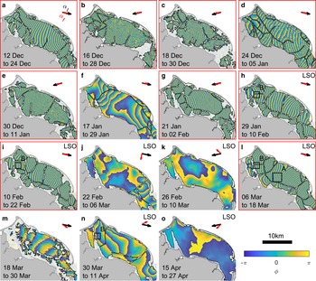
Of the 15 Sentinel 1 interferograms which maintain adequate coherence across Elson Lagoon for analysis (Fig. 5), ten contain RSVPs in which the phase gradient is monotonic in the look direction, meeting our criteria for assuming predominantly horizontal motion as discussed in Section 4. Of these ten interferograms (Figs 5a–e, g–i, l, m), there are nine in which mean α _f across Elson Lagoon remains near-parallel to α _l ($\vert \alpha _{{\rm diff}}\vert < 6^\circ$). These nine interferograms, outlined in red in Figure 5, include interferograms from both ascending and descending orbits, some of which overlap in time by several days.

Figure 5.

All 15 analyzed S1 interferograms over Elson Lagoon. Black arrows mark the mean look direction, α _l, from each pixel in the lagoon to the satellite. Red arrows mark the average azimuth direction of the phase gradient, α _f, within the lagoon. Red outlines highlight the nine interferograms (a–e, g–i, l) in which α _f remains near-parallel to α _l. Interferograms annotated ‘LSO’ in the top-right corner are interferograms for which point strain measurements from the LSO corresponding with both the start and end points of the interferogram exist. Box labeled ‘A’ marks the location of detail plots shown in Figure 6. Boxes labeled ‘B’ mark the location of the detail plots shown in Figure 9.

We use the following reasoning to infer radial convergence is the single dominant deformation mode during these nine images.

1. (1) Rotational displacement cannot produce fringes in the observed orientation.

2. (2) Simple shear solutions would require implausibly large strains >10⁻¹ at locations where α _f switches from clockwise to counter-clockwise of α _l (e.g. Fig. 6 a), implying switches between left and right lateral shear (Fig. 6b). Strains of this magnitude would certainly lead to the formation of cracks or ridges recognizable in the underlying SAR imagery and diminished interferometric coherence, neither of which are observed.

3. (3) To maintain the near-parallel relationship between average α _f and α _l axial convergence and simple shear would have needed to change orientation in synchrony with look direction. Similarly, translation direction would have needed to reverse in tandem with changes in look direction. There is no physical reason for this to happen consistently, particularly given temporal overlap between some interferograms acquired with differing look directions.

Figure 6.

Details from the Sentinel 1 interferogram spanning 6–18 March 2019 (Fig. 5l, box ‘A’). (a) In the top-right portion of the panel, above the red dashed line, α _f (red arrows) points counter-clockwise of α _l (black arrows) indicating right lateral shear, but in the lower left portion, α _f points clockwise of α _l, indicating left lateral shear. (b) Inverse modeled relative displacements (black arrows) in this area show unrealistically large divergent displacements of several meters and correspond to unrealistically large strains >0.1 (color bar) in the zone of transition from right to left lateral shear.

This leaves radial displacement as the only plausible main deformation mode making a majority contribution to the nine interferograms outlined in red in Figure 5. Radial displacement produces fringes with α _f parallel to α _l, and is plausible over 12 d periods in the context of the sheltered, landlocked lagoon.

6.7 Addressing model ambiguity in the Chukchi Sea

The relationship between α _f and α _l in TDX interferograms over drifting pack ice in the Chukchi Sea is more heterogeneous than that in Elson Lagoon (Figs 10a, e, i). In total, 84% of pixels reside in RSVPs in which the phase gradient points counter-clockwise of the look direction, but there are several cases of adjacent regions exhibiting nearly opposite phase gradient directions (e.g. white ellipse in Fig. 10e). In total, 48% of pixels reside in RSVPs where α _f is near-perpendicular (±10°) to α _l, and α _f is near-parallel (±10°) to α _l within only one RSVP (containing 14% total pixel area).

We infer radial convergence is an unlikely contributor to these phase gradients as it can only produce phase gradients with α _f parallel to α _l. Additionally, we expect radial convergence to result from thermal rather than dynamic forcing. A 10 s interferogram interval is much shorter than expected timescales of both diurnal and synoptic temperature changes that could lead to such strains. This leaves rotation, translation, simple shear and axial convergence as plausible deformation modes.

The uniformity of phase gradients across Chukchi Sea RSVPs suggests rigid motions are the most likely contributors. We expect non-rigid deformations to exhibit spatial variability, with largest magnitudes nearest to locations of contact with other RSVPs. Before ruling out non-rigid motion entirely, however, we pursue two, two-mode inversions: one combining translation and rotation, and one combining simple shear and axial convergence.

Translation and rotation produce nearly orthogonal fringes, allowing us to confidently separate their contributions to the phase gradient. We model the entire look parallel component of the phase gradient as the result of translation, and the entire look-perpendicular component of the phase gradient as the result of rotation.

Simple shear and axial convergence can produce fringes in any orientation. We lack independent measurements to quantitatively inform prescription of orientation or magnitude of either mode. Instead, we explore inverse solutions corresponding with all possible combinations of 50 shear orientations and 50 axial convergence orientations evenly spaced between −90° and 90°. The axial symmetry of these modes makes inclusion of orientations beyond this range redundant.

Maximum principal strains calculated from non-rigid model results approach infinity where α _f due to shear approaches α _l or α _f due to convergence approaches α_l ± π/2. However, minimum primary principal strains are finite, giving a meaningful floor to possible non-rigid strain magnitude in each RSVP. Across the three TDX interferograms analyzed, the 5th and 95th percentiles of minimum principal strain are −4.19 × 10⁻⁵ and 7.64 × 10⁻⁵. Over 10 s intervals we expect observed non-rigid strain to be primarily elastic, requiring a proportional change in stress. Assuming cold ice with an elastic modulus on the order of 10⁹ Pa, this proportional stress would be on the order of 10⁴ Pa (Timco and Weeks, Reference Timco and Weeks2010). This is the same order of magnitude as the largest observed stresses in in situ sea ice (e.g. Richter-Menge and others, Reference Richter-Menge, McNutt, Overland and Kwok2002; Parno and others, Reference Parno2022). The ice cannot support such stress changes over 10 s intervals over such large areas and remain intact, so the TDX interferograms cannot be the result of non-rigid deformation.