
 CD¯
CD¯ CD¯f
CD¯f CD¯p
CD¯p





1. Introduction
Understanding the motion mismatch between fluid flow and solid particles submerged in it is of vital importance in numerous natural and engineering processes, ranging from the sediment transport in rivers and seepage flow in soils to the mixing efficiency of industrial procedures. Due to the difficulties in measuring particle shapes with irregularities manifested by multi-scaled roughness, most relevant publications on these fluid–particle interactions consider ideal spheres. Pioneering works by Poisson (Reference Poisson1832), Green (Reference Green1835) and Stokes (Reference Stokes1845, Reference Stokes1851) laid the foundation for the study of the drag coefficient $C_{\!D}={F_{\!D}}/{(({1}/{2})\rho _{\!f}| \boldsymbol{u}_{\infty }| ^{2}A)}$
, where
$C_{\!D}={F_{\!D}}/{(({1}/{2})\rho _{\!f}| \boldsymbol{u}_{\infty }| ^{2}A)}$
, where $F_{\!D}$
is the drag force,
$F_{\!D}$
is the drag force, $\rho _{\!f}$
is the fluid density,
$\rho _{\!f}$
is the fluid density, $| \boldsymbol{u}_{\infty }|$
is the terminal or free-stream velocity of the fluid, and
$| \boldsymbol{u}_{\infty }|$
is the terminal or free-stream velocity of the fluid, and $A$
is the referenced area. This drag coefficient on spheres has been extensively investigated through experimental, numerical and analytical approaches for both steady (Oseen Reference Oseen1910) and unsteady (Clift, Grace & Weber Reference Clift, Grace and Weber1978) flows. Given the importance of irregular shapes of natural grains and their orientations, Oberbeck (Reference Oberbeck1876) used the Stokes stream function under the assumption of negligible advection to derive the first approximation of
$A$
is the referenced area. This drag coefficient on spheres has been extensively investigated through experimental, numerical and analytical approaches for both steady (Oseen Reference Oseen1910) and unsteady (Clift, Grace & Weber Reference Clift, Grace and Weber1978) flows. Given the importance of irregular shapes of natural grains and their orientations, Oberbeck (Reference Oberbeck1876) used the Stokes stream function under the assumption of negligible advection to derive the first approximation of $C_{\!D}$
for ellipsoids, or more specifically oblate and prolate spheroids with one circular crosswise area, at various orientations. Oseen (Reference Oseen1915) extended this work by providing a higher-order approximation for the disk with the flow perpendicular to its flat surfaces. The two classical methods proposed by Stokes and Oseen have later been combined to derive more robust solutions of aspherical, yet symmetrical grains (Proudman & Pearson Reference Proudman and Pearson1957; Breach Reference Breach1961; Batchelor Reference Batchelor1970). Nevertheless, the progress of these analytical derivations and their following improvements are rooted in the two minimal conditions: (i) low Reynolds number
$C_{\!D}$
for ellipsoids, or more specifically oblate and prolate spheroids with one circular crosswise area, at various orientations. Oseen (Reference Oseen1915) extended this work by providing a higher-order approximation for the disk with the flow perpendicular to its flat surfaces. The two classical methods proposed by Stokes and Oseen have later been combined to derive more robust solutions of aspherical, yet symmetrical grains (Proudman & Pearson Reference Proudman and Pearson1957; Breach Reference Breach1961; Batchelor Reference Batchelor1970). Nevertheless, the progress of these analytical derivations and their following improvements are rooted in the two minimal conditions: (i) low Reynolds number ${\textit{Re}}=({\rho _{\!f}\left| \boldsymbol{u}_{\infty }\right| d_{\textit{eq}}})/{\mu }$
, with
${\textit{Re}}=({\rho _{\!f}\left| \boldsymbol{u}_{\infty }\right| d_{\textit{eq}}})/{\mu }$
, with $d_{\textit{eq}}$
being the diameter of a volume-equivalent sphere, and
$d_{\textit{eq}}$
being the diameter of a volume-equivalent sphere, and $\mu$
being the dynamic viscosity, and (ii) ideal symmetrical grains immersed in the flow. The least controversy arises for the sphere in Stokes or creeping flow (
$\mu$
being the dynamic viscosity, and (ii) ideal symmetrical grains immersed in the flow. The least controversy arises for the sphere in Stokes or creeping flow ( ${\textit{Re}}\ll 1$
), where inertial effects vanish, and the contributions of the pressure and viscous stresses to the drag are analytically formulated:
${\textit{Re}}\ll 1$
), where inertial effects vanish, and the contributions of the pressure and viscous stresses to the drag are analytically formulated:
 \begin{equation} C_{\!D}=f(\textit{Re})=\underset{\text{pressure}}{\underbrace{8/\textit{Re}}}+\underset{\text{viscosity}}{\underbrace{16/\textit{Re}}}. \end{equation}
Such mechanics have underpinned various subsurface transport processes, e.g. microplastics transport in soils (Horton & Dixon Reference Horton and Dixon2018), and biological flows, e.g. cellular migration in tissues (Wilson Reference Wilson1978).
Building on the above-mentioned theoretical foundations, numerical and experimental investigations can be conducted to address the limitations of the two simplifications. However, empirically relating $C_{\!D}$
to
$C_{\!D}$
to ${\textit{Re}}$
remains challenging, even for spheres within the entire subcritical regime (Goossens Reference Goossens2019). Although the ellipsoidal shapes and the orientational dependence have been introduced (Zastawny et al. Reference Zastawny, Mallouppas, Zhao and van Wachem2012; Sanjeevi & Padding Reference Sanjeevi and Padding2017; Fröhlich et al. Reference Fröhlich, Meinke and Schröder2020), another simplification holds that the flow is parallel to one of the three symmetrical planes crossed by two of the three semi-axes. This implies that within the fluid domain, the grain has only one rotation angle in the spherical coordinate system referenced from its centre and semi-axes. To examine the orientation dependence of spheroids, Sanjeevi & Padding (Reference Sanjeevi and Padding2017) performed simulations via the lattice Boltzmann method. They found that for prolate spheroids at finite
${\textit{Re}}$
remains challenging, even for spheres within the entire subcritical regime (Goossens Reference Goossens2019). Although the ellipsoidal shapes and the orientational dependence have been introduced (Zastawny et al. Reference Zastawny, Mallouppas, Zhao and van Wachem2012; Sanjeevi & Padding Reference Sanjeevi and Padding2017; Fröhlich et al. Reference Fröhlich, Meinke and Schröder2020), another simplification holds that the flow is parallel to one of the three symmetrical planes crossed by two of the three semi-axes. This implies that within the fluid domain, the grain has only one rotation angle in the spherical coordinate system referenced from its centre and semi-axes. To examine the orientation dependence of spheroids, Sanjeevi & Padding (Reference Sanjeevi and Padding2017) performed simulations via the lattice Boltzmann method. They found that for prolate spheroids at finite ${\textit{Re}}$
, the fluid-induced drag and lift forces depend on the inclination angle similarly to predictions in the Stokes regime (Happel & Brenner Reference Happel and Brenner1983). However, this correlation is less accurate for flat oblate spheroids with an aspect ratio – defined as the length ratio of semi-major axis
${\textit{Re}}$
, the fluid-induced drag and lift forces depend on the inclination angle similarly to predictions in the Stokes regime (Happel & Brenner Reference Happel and Brenner1983). However, this correlation is less accurate for flat oblate spheroids with an aspect ratio – defined as the length ratio of semi-major axis $\mathscr{a}$
to semi-minor axis
$\mathscr{a}$
to semi-minor axis $\mathscr{b}=\mathscr{a}(1-\epsilon )$
– of 4. This is because the analytical solution in Happel & Brenner (Reference Happel and Brenner1983) is based on spheroids with aspect ratio close to unity, allowing the omission of the high-order term, i.e.
$\mathscr{b}=\mathscr{a}(1-\epsilon )$
– of 4. This is because the analytical solution in Happel & Brenner (Reference Happel and Brenner1983) is based on spheroids with aspect ratio close to unity, allowing the omission of the high-order term, i.e. $\mathcal{O}(\epsilon ^{2})$
. Nevertheless, efforts continue to examine whether the analytics from minimal geometries can be applied to complicated shapes for the potential
$\mathcal{O}(\epsilon ^{2})$
. Nevertheless, efforts continue to examine whether the analytics from minimal geometries can be applied to complicated shapes for the potential $C_{\!D}$
prediction. Along this line, Vergara, Wei & Fuentes (Reference Vickers2024) found that
$C_{\!D}$
prediction. Along this line, Vergara, Wei & Fuentes (Reference Vickers2024) found that $C_{\!D}$
– altered by only one rotation angle of realistic shaped grains – conforms to a sine-squared law predicted from linearity of the Stokes equations even up to
$C_{\!D}$
– altered by only one rotation angle of realistic shaped grains – conforms to a sine-squared law predicted from linearity of the Stokes equations even up to ${\textit{Re}}=2000$
. To fully relieve the one-rotation-angle simplification in predicting
${\textit{Re}}=2000$
. To fully relieve the one-rotation-angle simplification in predicting $C_{\!D}$
of irregular, asymmetrical shapes, it is promising to correlate
$C_{\!D}$
of irregular, asymmetrical shapes, it is promising to correlate $A_{\!p}$
, the projected area to the flow direction, to
$A_{\!p}$
, the projected area to the flow direction, to $C_{\!D}$
. This pathway draws inspiration from the solid analytical formula for spheroidal shapes, as
$C_{\!D}$
. This pathway draws inspiration from the solid analytical formula for spheroidal shapes, as $A_{\!p}$
exhibits the two-rotation-angle dependence.
$A_{\!p}$
exhibits the two-rotation-angle dependence.
Experimental results are preferable in practical applications due to the involvement of all-natural particle shapes. Wadell (Reference Wadell1934a
,
Reference Wadellb
) realised the importance of the particle area, including $A_{\!p}$
and surface area
$A_{\!p}$
and surface area $S_{a}$
, in determining both the pressure and the friction drag. The drag coefficient
$S_{a}$
, in determining both the pressure and the friction drag. The drag coefficient $C_{\!D}$
was correlated to particle shape parameters, including circularity
$C_{\!D}$
was correlated to particle shape parameters, including circularity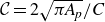 $\mathcal{C}=2\sqrt{\pi\! A_{\!p}}/C$
, and sphericity
$\mathcal{C}=2\sqrt{\pi\! A_{\!p}}/C$
, and sphericity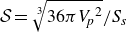 $\mathcal{S}=\sqrt[3]{36\pi {V_{\!p}}^{2}}/S_{s}$
, where
$\mathcal{S}=\sqrt[3]{36\pi {V_{\!p}}^{2}}/S_{s}$
, where $C$
is the perimeter of the projected area,
$C$
is the perimeter of the projected area, $V_{\!p}$
is the enclosed volume, and
$V_{\!p}$
is the enclosed volume, and $S_{s}$
is the surface area of the volume-equivalent sphere. Since then, plentiful studies have been dedicated to
$S_{s}$
is the surface area of the volume-equivalent sphere. Since then, plentiful studies have been dedicated to
 \begin{equation} C_{\!D}=f(Re,\underset{\text{shape indices}}{\underbrace{\mathcal{P}_{1}\ldots \mathcal{P}_{n}}}). \end{equation}
Various fitting formulas can be referred to some in-depth review papers, such as Loth (Reference Loth2008), Bagheri & Bonadonna (Reference Bagheri and Bonadonna2016) and Michaelides & Feng (Reference Michaelides and Feng2023). However, Hölzer & Sommerfeld (Reference Hughes and Mallet2008) claim that empirical and semi-empirical drag coefficient models on irregularly shaped grains could yield significant prediction errors, i.e. more than 1000 %, when used for other experimental data sets. The substantial uncertainty in drag coefficient predictions can be attributed to two primary factors. First, the shape indices in these equations are single-scaled, lacking a quantification of full-scaled grain morphology. Wadell himself classified the grain morphology into three aspects: the general form for grain dimensions, the roundness for local corners, and the fine roughness for small features (Wadell Reference Wadell1932, Reference van Wachem, Zastawny, Zhao and Mallouppas1935). Second, in typical experimental set-ups where the terminal settling velocity of a natural grain in a quiescent fluid is measured, the irregular-shaped grain continually adjusts its orientation. This orientation changes $A_{\!p}$
, thereby influencing
$A_{\!p}$
, thereby influencing $C_{\!D}$
. Consequently, the settling grain experiment without control of its rotation could yield great uncertainty in
$C_{\!D}$
. Consequently, the settling grain experiment without control of its rotation could yield great uncertainty in $C_{\!D}$
. Moreover, in the creeping regime, the departure of a grain from a sphere has been generally and intuitively considered to increase
$C_{\!D}$
. Moreover, in the creeping regime, the departure of a grain from a sphere has been generally and intuitively considered to increase $C_{\!D}$
. In the context of rough channel flows, distinct behaviour is exhibited. For the hydraulically smooth regime of low
$C_{\!D}$
. In the context of rough channel flows, distinct behaviour is exhibited. For the hydraulically smooth regime of low ${\textit{Re}}$
, surface roughness is entirely submerged within the viscous layer, presenting little impact on skin friction and the drag coefficient (Kadivar, Tormey & McGranaghan Reference Kadivar, Tormey and McGranaghan2021). Conversely, in the rough flow regime of median
${\textit{Re}}$
, surface roughness is entirely submerged within the viscous layer, presenting little impact on skin friction and the drag coefficient (Kadivar, Tormey & McGranaghan Reference Kadivar, Tormey and McGranaghan2021). Conversely, in the rough flow regime of median ${\textit{Re}}$
, surface roughness could induce drag reduction (Choi, Jeon & Kim Reference Chéron, Evrard and van Wachem2008). While wall-bounded roughness at high Reynolds number is often deemed to be composed of dense overlapped polydisperse spherical caps, parametrised by an equivalent sand-grain roughness
${\textit{Re}}$
, surface roughness could induce drag reduction (Choi, Jeon & Kim Reference Chéron, Evrard and van Wachem2008). While wall-bounded roughness at high Reynolds number is often deemed to be composed of dense overlapped polydisperse spherical caps, parametrised by an equivalent sand-grain roughness $k_{s}$
(Nikuradse Reference Nikuradse1933), the present study is strictly confined to the Stokes limit (
$k_{s}$
(Nikuradse Reference Nikuradse1933), the present study is strictly confined to the Stokes limit ( ${\textit{Re}}\ll 1$
) for an isolated rough grain in an unbounded domain. For rough channel flow at high
${\textit{Re}}\ll 1$
) for an isolated rough grain in an unbounded domain. For rough channel flow at high ${\textit{Re}}$
, the single-grain Stokes problem is a minimal case – a mechanistically clean setting that removes inertia, turbulence and inter-element interactions – to probe how multi-scale morphology and its orientation redistribute pressure and friction drag at the grain scale.
${\textit{Re}}$
, the single-grain Stokes problem is a minimal case – a mechanistically clean setting that removes inertia, turbulence and inter-element interactions – to probe how multi-scale morphology and its orientation redistribute pressure and friction drag at the grain scale.
In this study, we aim to investigate how the grain roughness impacts the drag coefficient of a single grain in a creeping flow. After analytically deriving the relation between projected area and drag coefficient for ellipsoidal grains, we conduct over 2000 direct numerical simulations (DNS) for both ellipsoidal and rough grains. We then assess whether the solution derived for minimal shapes can be extended to more complicated geometries. Rough shapes are generated based on spherical harmonics (SH), exhibiting multi-scale morphology features effectively captured by two compressed shape parameters (fractal dimension and root mean square roughness). Each grain is rotated to 51 orientations by both zenith and azimuth angles, while the flow direction is unchanged, to discuss the morphological and orientational universality in drag coefficients. The rest of the paper is organised as follows. In § 2, for the numerical methods, we detail how rough grain shapes are depicted, and the finite element scheme to compute fluid–grain interaction stress. Section 3 presents the analytical solution for the dependence of the drag coefficient on projected area of both spheroidal and ellipsoidal grains. In § 4, we examine the applicability of the derived power law to more complex shapes, as well as other macro results, including orientation-dependent drag coefficient and its two corresponding contributions from skin friction and pressure drag. Subsequently, in § 5 the microanalysis on frictional and pressure distributions on rough grain surfaces is conducted to explain the departure of macro drag coefficients from those of their volume-equivalent spheres. Discussions are carried out in § 6 about how the results can be utilised to explain the drag paradox where drag enhancement is commonly observed in settling grain experiments popular in geophysics. Finally, this section also concludes the study by summarising the key insights and implications of our research.
2. Numerical methods
2.1. Grain shape generation and description
In concurrent studies on drag coefficients of grains, the ideal geometry with fully convex shapes is of high priority. However, realistic grain surfaces usually demonstrate fractality manifested by irregular tortuosity over a wide range of length scales (Barclay & Buckingham Reference Barclay and Buckingham2009). In this study, we adopt the inverse analysis of SH with prescribed power spectrum to generate such multi-scaled morphology features (Wei et al. Reference Wei, Wang, Pereira and Gan2021); the power spectrum is enriched with fractality and root mean square roughness. A rough grain constructed with star-shaped surficial points can be approximated using the SH function ${Y}_{n}^{m}(\theta ,\varphi )$
, via denoting its radial length in the spherical coordinate system as
${Y}_{n}^{m}(\theta ,\varphi )$
, via denoting its radial length in the spherical coordinate system as
 \begin{equation}r(\theta ,\varphi )=\sum\nolimits_{n=0}^{\infty }\sum\nolimits_{m=-n}^{n}{c}_{n}^{m}\,{Y}_{n}^{m}(\theta ,\varphi ),\end{equation}
where $\theta \in [0,\pi ]$
and
$\theta \in [0,\pi ]$
and $\varphi \in (0,2\pi ]$
are the latitudinal and longitudinal coordinates, respectively, and
$\varphi \in (0,2\pi ]$
are the latitudinal and longitudinal coordinates, respectively, and ${c}_{n}^{m}$
are the SH coefficients of spherical wavenumber
${c}_{n}^{m}$
are the SH coefficients of spherical wavenumber $n$
and order
$n$
and order $m$
. With the help of Parseval’s theorem, at each SH frequency, the power spectrum is
$m$
. With the help of Parseval’s theorem, at each SH frequency, the power spectrum is $L_{n}=\|f_{n}\|=\sqrt{\sum_{m=-n}^{n}\|{c}_{n}^{m}\|^{2}}$
, with
$L_{n}=\|f_{n}\|=\sqrt{\sum_{m=-n}^{n}\|{c}_{n}^{m}\|^{2}}$
, with $\|\cdot\|$
being the L
2 norm. The average radius length
$\|\cdot\|$
being the L
2 norm. The average radius length $\overline{r}$
, equal to its
$\overline{r}$
, equal to its $c_{0}$
-determined sphere
$c_{0}$
-determined sphere $R_{0}$
, reads as
$R_{0}$
, reads as $\overline{r}\approx R_{0}=c_{0}\,Y_{0}(\theta ,\varphi )$
, where
$\overline{r}\approx R_{0}=c_{0}\,Y_{0}(\theta ,\varphi )$
, where $Y_{0}(\theta ,\varphi )=1/(2\sqrt{\pi })$
. To quantify how a rough grain surface is globally different from
$Y_{0}(\theta ,\varphi )=1/(2\sqrt{\pi })$
. To quantify how a rough grain surface is globally different from $\overline{r}$
, the relative roughness is defined as the ratio
$\overline{r}$
, the relative roughness is defined as the ratio $R_{r}=S_{q}/\overline{r}$
, i.e. the root mean square
$R_{r}=S_{q}/\overline{r}$
, i.e. the root mean square $S_{q}=\sqrt{(\sum_{n=1}^{\infty }\sum_{m=-n}^{n}\|{c}_{n}^{m}\|^{2})/(4\pi )}$
over
$S_{q}=\sqrt{(\sum_{n=1}^{\infty }\sum_{m=-n}^{n}\|{c}_{n}^{m}\|^{2})/(4\pi )}$
over $\overline{r}$
. With
$\overline{r}$
. With $R_{r}$
and
$R_{r}$
and $c_{0}$
in hand, the grain volume can be correspondingly determined as
$c_{0}$
in hand, the grain volume can be correspondingly determined as $V_{\!p}=c_{0}^{3}(1+3R_{r}^{2})/(6\sqrt{\pi })$
, which eases the definition of effective grain diameter
$V_{\!p}=c_{0}^{3}(1+3R_{r}^{2})/(6\sqrt{\pi })$
, which eases the definition of effective grain diameter $d_{\textit{eq}}=\sqrt[3]{6V_{\!p}/\pi }=c_{0}\sqrt[3]{1+3R_{r}^{2}}/\sqrt{\pi }$
; the grain surface area is approximately
$d_{\textit{eq}}=\sqrt[3]{6V_{\!p}/\pi }=c_{0}\sqrt[3]{1+3R_{r}^{2}}/\sqrt{\pi }$
; the grain surface area is approximately $S_{a}=c_{0}^{2}(1+\pi R_{r}^{\pi /2}D_{\!f}^{3.874})/20$
(Wei et al. Reference Wei, Wang, Pereira and Gan2021). Meanwhile, the multi-scale features – denoting how a rough grain surface is globally different from
$S_{a}=c_{0}^{2}(1+\pi R_{r}^{\pi /2}D_{\!f}^{3.874})/20$
(Wei et al. Reference Wei, Wang, Pereira and Gan2021). Meanwhile, the multi-scale features – denoting how a rough grain surface is globally different from $\overline{r}$
– can be characterised by fractal dimension
$\overline{r}$
– can be characterised by fractal dimension $D_{\!f}$
; it is originated from the logarithmic linear relations between
$D_{\!f}$
; it is originated from the logarithmic linear relations between $L_{n}$
and
$L_{n}$
and $n$
, i.e.
$n$
, i.e. $L_{n}\propto n^{\beta }$
, where
$L_{n}\propto n^{\beta }$
, where $\beta =-2H$
is the slope of the regression plot of
$\beta =-2H$
is the slope of the regression plot of $\log(L_{n})$
versus
$\log(L_{n})$
versus $\log(n)$
, and
$\log(n)$
, and $H$
is the Hurst coefficient used to calculate
$H$
is the Hurst coefficient used to calculate $D_{\!f}=3-H$
(Russ Reference Russ2013). With increasing
$D_{\!f}=3-H$
(Russ Reference Russ2013). With increasing $n$
, more and more fine surficial details could be depicted. Considering the extremely low
$n$
, more and more fine surficial details could be depicted. Considering the extremely low ${\textit{Re}}=10^{-5}$
,
${\textit{Re}}=10^{-5}$
, $n_{max}=15$
is fixed considering the related cut-off or minimum wavelength
$n_{max}=15$
is fixed considering the related cut-off or minimum wavelength $\lambda (n)={\pi }\overline{r}/n={\pi }\overline{r}/15$
according to the famous Jean’s formula.
$\lambda (n)={\pi }\overline{r}/n={\pi }\overline{r}/15$
according to the famous Jean’s formula.
Rough grain morphology features and the numerical set-up. (a) Various rough grains in the $R_{r}$
–
$R_{r}$
– $D_{\!f}$
space. The colour bar represents the ratio of the grain radial length
$D_{\!f}$
space. The colour bar represents the ratio of the grain radial length $r(\theta ,\varphi )$
to its mean radial length
$r(\theta ,\varphi )$
to its mean radial length $\overline{r}$
. (b) The schematic of a free stream passing a rough grain. Here,
$\overline{r}$
. (b) The schematic of a free stream passing a rough grain. Here, $\boldsymbol{p}_{{1}}$
,
$\boldsymbol{p}_{{1}}$
, $\boldsymbol{p}_{{2}}$
, and
$\boldsymbol{p}_{{2}}$
, and $\boldsymbol{p}_{{3}}$
are directions of the longer semi-major, median and semi-minor axes of the rough grain, respectively; they are parallel with the global
$\boldsymbol{p}_{{3}}$
are directions of the longer semi-major, median and semi-minor axes of the rough grain, respectively; they are parallel with the global $x$
-,
$x$
-, $y$
- and
$y$
- and $z$
-axes, respectively, of which the positive directions are indicated by the arrow directions in the left bottom corner. The purple solid line denotes the semi-major grain axis after a rotation around the centre
$z$
-axes, respectively, of which the positive directions are indicated by the arrow directions in the left bottom corner. The purple solid line denotes the semi-major grain axis after a rotation around the centre $O$
. Here,
$O$
. Here, $\boldsymbol{p}_{1}{'}$
is the vector of the semi-major axis
$\boldsymbol{p}_{1}{'}$
is the vector of the semi-major axis $\boldsymbol{p}_{{1}}$
after rotation, and
$\boldsymbol{p}_{{1}}$
after rotation, and $\boldsymbol{p}_{{1},\boldsymbol{xy}}{'}$
is its projection on the
$\boldsymbol{p}_{{1},\boldsymbol{xy}}{'}$
is its projection on the $\boldsymbol{x}$
–
$\boldsymbol{x}$
– $y$
plane. Also,
$y$
plane. Also, $\Theta \in [0,\pi ]$
, defined as the angle between
$\Theta \in [0,\pi ]$
, defined as the angle between $\boldsymbol{p}_{{3}}$
or
$\boldsymbol{p}_{{3}}$
or $\boldsymbol{z}$
and
$\boldsymbol{z}$
and $\boldsymbol{p}_{1}{'}$
, and
$\boldsymbol{p}_{1}{'}$
, and $\Phi \in [0,2\pi )$
, defined as the angle between
$\Phi \in [0,2\pi )$
, defined as the angle between $\boldsymbol{p}_{{1},\boldsymbol{xy}}{'}$
and
$\boldsymbol{p}_{{1},\boldsymbol{xy}}{'}$
and $\boldsymbol{p}_{{1}}$
or
$\boldsymbol{p}_{{1}}$
or $\boldsymbol{x}$
, are the zenith angle and azimuth angle of
$\boldsymbol{x}$
, are the zenith angle and azimuth angle of $\boldsymbol{p}_{1}{'}$
, respectively;
$\boldsymbol{p}_{1}{'}$
, respectively; $\vartheta$
is the angle crossed by
$\vartheta$
is the angle crossed by $\boldsymbol{p}_{1}{'}$
and the opposite direction of the flow, which is indicated by the blue arrow. (c) Mesh sensitivity study on the benchmark case, i.e. Stokes drag of a sphere. Here,
$\boldsymbol{p}_{1}{'}$
and the opposite direction of the flow, which is indicated by the blue arrow. (c) Mesh sensitivity study on the benchmark case, i.e. Stokes drag of a sphere. Here, $h$
is the mesh size, and
$h$
is the mesh size, and $R_{0}$
is the volume-equivalent sphere radius. The selected mesh size for the systematic study is indicated by the star.
$R_{0}$
is the volume-equivalent sphere radius. The selected mesh size for the systematic study is indicated by the star.

As illustrated in figure 1(a), where $c_{0}=2\sqrt{\pi }$
is set to depict a unit sphere with
$c_{0}=2\sqrt{\pi }$
is set to depict a unit sphere with $\overline{r}=1$
, higher
$\overline{r}=1$
, higher $R_{r}$
and
$R_{r}$
and $D_{\!f}$
could induce more irregularities in general shapes and local waviness, respectively. For natural granular materials, the value of
$D_{\!f}$
could induce more irregularities in general shapes and local waviness, respectively. For natural granular materials, the value of $D_{\!f}$
for quartz sands is mostly in the range
$D_{\!f}$
for quartz sands is mostly in the range $[2.1,2.3]$
, and the value of
$[2.1,2.3]$
, and the value of $R_{r}$
is approximately 0.1 (Wei et al. Reference Wei, Wang, Pereira and Gan2021). Extremely fine values of
$R_{r}$
is approximately 0.1 (Wei et al. Reference Wei, Wang, Pereira and Gan2021). Extremely fine values of $(R_{r},D_{\!f})=(0.01,2.05)$
could be encountered in artificial spherical particulates, such as glass beads; ultra-high
$(R_{r},D_{\!f})=(0.01,2.05)$
could be encountered in artificial spherical particulates, such as glass beads; ultra-high $R_{r}\gt 0.15$
and
$R_{r}\gt 0.15$
and $D_{\!f}\gt 2.4$
could appear in some macromolecules and human brains (Yotter et al. Reference Yotter, Thompson, Nenadic and Gaser2010). Without loss of generality, a series of simulations are conducted for rough grains with
$D_{\!f}\gt 2.4$
could appear in some macromolecules and human brains (Yotter et al. Reference Yotter, Thompson, Nenadic and Gaser2010). Without loss of generality, a series of simulations are conducted for rough grains with $R_{r}\in [0,0.35]$
and
$R_{r}\in [0,0.35]$
and $D_{\!f}\in [2.1,2.5]$
. The classical shape parameters, including ratio (
$D_{\!f}\in [2.1,2.5]$
. The classical shape parameters, including ratio ( $\mathcal{A}_{\mathscr{r}}$
), elongation (
$\mathcal{A}_{\mathscr{r}}$
), elongation ( $\mathcal{E}_{\mathscr{i}}$
), flatness (
$\mathcal{E}_{\mathscr{i}}$
), flatness ( $\mathcal{F}_{\mathscr{i}}$
), roundness (
$\mathcal{F}_{\mathscr{i}}$
), roundness ( $\mathcal{R}$
), sphericity (
$\mathcal{R}$
), sphericity ( $\mathcal{S}$
) and convexity (
$\mathcal{S}$
) and convexity ( $\mathcal{C}_{\mathcal{X}}$
), of these aspherical grain shapes are demonstrated in tables 1, 2, 3, 4, 5 and 6 of Appendix A. The specific definitions of these shape indices can be found in Zhao & Wang (Reference Zhao and Wang2016). Notably,
$\mathcal{C}_{\mathcal{X}}$
), of these aspherical grain shapes are demonstrated in tables 1, 2, 3, 4, 5 and 6 of Appendix A. The specific definitions of these shape indices can be found in Zhao & Wang (Reference Zhao and Wang2016). Notably, $R_{r}$
cannot increase infinitely, as higher
$R_{r}$
cannot increase infinitely, as higher $R_{r}$
could generate negative
$R_{r}$
could generate negative $r(\theta ,\varphi )$
, which is contrary to the star-like shape reconstructed by SH; when expanded in the spherical coordinate system,
$r(\theta ,\varphi )$
, which is contrary to the star-like shape reconstructed by SH; when expanded in the spherical coordinate system, $r(\theta ,\varphi )$
is an injective rather than bijective function. As a supplement, the ratio of minimum to maximum
$r(\theta ,\varphi )$
is an injective rather than bijective function. As a supplement, the ratio of minimum to maximum $r(\theta ,\varphi )$
is also provided as a newly defined aspect ratio
$r(\theta ,\varphi )$
is also provided as a newly defined aspect ratio $\mathcal{A}_{\mathcal{R}}=\min _{} (r(\theta ,\varphi ))/\max _{} (r(\theta ,\varphi ))$
in table 7 of Appendix A. For ellipsoids,
$\mathcal{A}_{\mathcal{R}}=\min _{} (r(\theta ,\varphi ))/\max _{} (r(\theta ,\varphi ))$
in table 7 of Appendix A. For ellipsoids, $\mathcal{A}_{\mathcal{R}}=\mathcal{A}_{\mathscr{r}}$
, which is not the case for rough grains in figure 1(a).
$\mathcal{A}_{\mathcal{R}}=\mathcal{A}_{\mathscr{r}}$
, which is not the case for rough grains in figure 1(a).
To determine $C_{\!D}$
for a rough grain, a numerical model is developed in the next subsection. The analysis of rotational dependence for drag coefficients is performed with two rotations relative to the flow direction: azimuthal rotation
$C_{\!D}$
for a rough grain, a numerical model is developed in the next subsection. The analysis of rotational dependence for drag coefficients is performed with two rotations relative to the flow direction: azimuthal rotation $\Phi$
and polar rotation
$\Phi$
and polar rotation $\Theta$
as in figure 1(b). Principal component analysis (PCA) is also utilised to determine major, median and minor axes with respect to
$\Theta$
as in figure 1(b). Principal component analysis (PCA) is also utilised to determine major, median and minor axes with respect to $\boldsymbol{p}_{{1}}$
,
$\boldsymbol{p}_{{1}}$
, $\boldsymbol{p}_{{2}}$
and
$\boldsymbol{p}_{{2}}$
and $\boldsymbol{p}_{{3}}$
(Fonseca Reference Fonseca2011), respectively. Notably, minimum and maximum
$\boldsymbol{p}_{{3}}$
(Fonseca Reference Fonseca2011), respectively. Notably, minimum and maximum $A_{\!p}$
are respectively represented by projected areas vertical to
$A_{\!p}$
are respectively represented by projected areas vertical to $\boldsymbol{p}_{{1}}$
and
$\boldsymbol{p}_{{1}}$
and $\boldsymbol{p}_{{3}}$
. In total, 49 periodic rotations from an initially random orientation, of both
$\boldsymbol{p}_{{3}}$
. In total, 49 periodic rotations from an initially random orientation, of both $\Phi$
and
$\Phi$
and $\Theta$
from
$\Theta$
from $0$
to
$0$
to $2\pi$
with gap
$2\pi$
with gap ${\pi }/{3}$
, plus 2 featured directions (
${\pi }/{3}$
, plus 2 featured directions ( $\boldsymbol{p}_{{1}}$
and
$\boldsymbol{p}_{{1}}$
and $\boldsymbol{p}_{{3}}$
) are considered for each morphology. A sensitivity study of the orientation number has been performed (see figure 9(c) of Appendix B), suggesting that the statistical features of drag can be captured with this orientation number (
$\boldsymbol{p}_{{3}}$
) are considered for each morphology. A sensitivity study of the orientation number has been performed (see figure 9(c) of Appendix B), suggesting that the statistical features of drag can be captured with this orientation number ( $N=51$
).
$N=51$
).
2.2. Governing equations and numerical configuration
When relative movement occurs between the grain and its surrounding fluid, it experiences a resultant force. The force may not align with the flow due to the asymmetric morphology, and can be split into streamwise drag force and spanwise lift force. Here, our study exclusively focuses on the drag force. The total drag force $F_{\!D}$
is obtained by a surface integral of the total stress
$F_{\!D}$
is obtained by a surface integral of the total stress $\boldsymbol{\sigma }$
on the grain surface
$\boldsymbol{\sigma }$
on the grain surface $\partial \Omega$
projected on streamwise direction
$\partial \Omega$
projected on streamwise direction $\boldsymbol{e}_{s}$
:
$\boldsymbol{e}_{s}$
:

Here, $\boldsymbol{\sigma }=-p\boldsymbol{I}+\boldsymbol{\tau }$
is a sum of the pressure tensor
$\boldsymbol{\sigma }=-p\boldsymbol{I}+\boldsymbol{\tau }$
is a sum of the pressure tensor $p\boldsymbol{I}$
and the shear stress
$p\boldsymbol{I}$
and the shear stress $\boldsymbol{\tau }=[\boldsymbol{\nabla }\boldsymbol{u}+(\boldsymbol{\nabla }\boldsymbol{u})^{\rm T}]$
, where
$\boldsymbol{\tau }=[\boldsymbol{\nabla }\boldsymbol{u}+(\boldsymbol{\nabla }\boldsymbol{u})^{\rm T}]$
, where $\boldsymbol{u}$
is flow velocity. Therefore, the total drag force can be considered to be composed of two components, i.e. the skin friction
$\boldsymbol{u}$
is flow velocity. Therefore, the total drag force can be considered to be composed of two components, i.e. the skin friction
 and the pressure drag
 . We define ${C}_{\!D}^{p}$
and
${C}_{\!D}^{p}$
and ${C}_{\!D}^{f}$
using
${C}_{\!D}^{f}$
using ${F}_{\!D}^{p}$
and
${F}_{\!D}^{p}$
and ${F}_{\!D}^{f}$
in the same manner as
${F}_{\!D}^{f}$
in the same manner as $C_{\!D}={F_{\!D}}/{(({1}/{2})\rho _{\!f}| \boldsymbol{u}_{\infty }| ^{2}A_{\!p})}$
, with
$C_{\!D}={F_{\!D}}/{(({1}/{2})\rho _{\!f}| \boldsymbol{u}_{\infty }| ^{2}A_{\!p})}$
, with $A_{\!p}$
being the projected area, corresponding to effects of pressure and viscous stresses on drag, respectively. For all grains in this study,
$A_{\!p}$
being the projected area, corresponding to effects of pressure and viscous stresses on drag, respectively. For all grains in this study, ${\textit{Re}}={\rho _{\!f}}U_{\infty }d_{\textit{eq}}/\mu _{\!f}$
is approximately
${\textit{Re}}={\rho _{\!f}}U_{\infty }d_{\textit{eq}}/\mu _{\!f}$
is approximately $10^{-5}\ll 1$
, where
$10^{-5}\ll 1$
, where $\rho _{\!f}$
,
$\rho _{\!f}$
, $\mu _{\!f}$
and
$\mu _{\!f}$
and $U_{\infty }$
are respectively the density, viscosity and relative velocity of the fluid. In such a Stokesian limit,
$U_{\infty }$
are respectively the density, viscosity and relative velocity of the fluid. In such a Stokesian limit, $C_{\!D}={24}/{\textit{Re}}$
. We henceforth use the Reynolds-normalised drag coefficients
$C_{\!D}={24}/{\textit{Re}}$
. We henceforth use the Reynolds-normalised drag coefficients $C_{\overline{D}}={\textit{Re}}\,C_{\!D}$
,
$C_{\overline{D}}={\textit{Re}}\,C_{\!D}$
, ${C}_{\overline{D}}^{p}={\textit{Re}}\,{C}_{\!D}^{p}$
and
${C}_{\overline{D}}^{p}={\textit{Re}}\,{C}_{\!D}^{p}$
and ${C}_{\overline{D}}^{f}={\textit{Re}}\,{C}_{\!D}^{f}$
; for a sphere in the Stokes limit,
${C}_{\overline{D}}^{f}={\textit{Re}}\,{C}_{\!D}^{f}$
; for a sphere in the Stokes limit, $C_{\overline{D}}=24$
,
$C_{\overline{D}}=24$
, ${C}_{\overline{D}}^{p}=8$
and
${C}_{\overline{D}}^{p}=8$
and ${C}_{\overline{D}}^{f}=16$
. The insensitivity of
${C}_{\overline{D}}^{f}=16$
. The insensitivity of $C_{\overline{D}}$
,
$C_{\overline{D}}$
, ${C}_{\overline{D}}^{p}$
and
${C}_{\overline{D}}^{p}$
and ${C}_{\overline{D}}^{f}$
to the selected Reynolds number
${C}_{\overline{D}}^{f}$
to the selected Reynolds number ${\textit{Re}}\approx 10^{-5}$
is confirmed via simulations for spherical, ellipsoidal and rough grains, as indicated in figure 9(d) of Appendix B.
${\textit{Re}}\approx 10^{-5}$
is confirmed via simulations for spherical, ellipsoidal and rough grains, as indicated in figure 9(d) of Appendix B.
The twofold integrals in (2.2) can be obtained by solving the continuity and momentum equations. No separation of the boundary layer occurs, and the flow field can be adequately described by the Stokes equations
 \begin{equation}\boldsymbol{\nabla }\boldsymbol{\cdot }\boldsymbol{u}=0 \quad\text{and}\quad \boldsymbol{\nabla }\boldsymbol{\cdot }\boldsymbol{\tau }=\boldsymbol{\nabla }p.\end{equation}
In the DNS, lengths, velocities, stresses and forces are non-dimensionalised by $D_{\!p}$
,
$D_{\!p}$
, $U_{\infty }$
,
$U_{\infty }$
, ${\mu _{\!f}}U_{\infty }/d_{\textit{eq}}$
and
${\mu _{\!f}}U_{\infty }/d_{\textit{eq}}$
and ${\mu _{\!f}}U_{\infty }d_{\textit{eq}}$
, respectively. The flow region, as shown in figure 1(b), is a rectangular domain with
${\mu _{\!f}}U_{\infty }d_{\textit{eq}}$
, respectively. The flow region, as shown in figure 1(b), is a rectangular domain with $[L_{x},L_{y},L_{z}]=[18d_{\textit{eq}},20d_{\textit{eq}},20d_{\textit{eq}}]$
along, respectively, the streamwise (
$[L_{x},L_{y},L_{z}]=[18d_{\textit{eq}},20d_{\textit{eq}},20d_{\textit{eq}}]$
along, respectively, the streamwise ( $x$
-axis) and spanwise (
$x$
-axis) and spanwise ( $y$
- and
$y$
- and $z$
-axes) directions. A sensitivity study of the domain size was conducted on the roughest grain with
$z$
-axes) directions. A sensitivity study of the domain size was conducted on the roughest grain with $(R_{r},D_{\!f})=(0.35,2.5)$
(see figure 9(b) of Appendix B), and it is confirmed that with the selected
$(R_{r},D_{\!f})=(0.35,2.5)$
(see figure 9(b) of Appendix B), and it is confirmed that with the selected $[L_{x},L_{y},L_{z}]$
, the domain size effect is negligible. At the inlet, outlet and sidewalls, a translational velocity
$[L_{x},L_{y},L_{z}]$
, the domain size effect is negligible. At the inlet, outlet and sidewalls, a translational velocity $U_{{\infty }}$
along the streamwise direction is imposed. The grain remains stationary at the domain centre, and a no-slip boundary condition is imposed on the grain surface. The numerical settings are verified by the very good agreement between theoretical and simulated
$U_{{\infty }}$
along the streamwise direction is imposed. The grain remains stationary at the domain centre, and a no-slip boundary condition is imposed on the grain surface. The numerical settings are verified by the very good agreement between theoretical and simulated $C_{\!D}$
of perfectly smoothed spheres in figure 1(c).
$C_{\!D}$
of perfectly smoothed spheres in figure 1(c).
The finite element scheme with the boundary-fitted method in COMSOL Multiphysics® is adopted to solve (2.3). The fluid domain is discretised using more than 600 000 tetrahedron elements with mixed-order shape functions, i.e. Taylor–Hood elements (Taylor & Hood Reference Taylor and Hood1973), to guarantee the divergence stability. The stationary solution of the equation set is obtained by solving a saddle point problem. For the detailed discussion of the weak form and corresponding numerical stabilisation techniques, one can refer to Hughes & Mallet (Reference Hölzer and Sommerfeld1986) and Hauke & Hughes (Reference Hauke and Hughes1994). The element size $h$
is grossly identical to that of generic triangular meshes on grain surfaces:
$h$
is grossly identical to that of generic triangular meshes on grain surfaces: $h=1.2\times {10^{-2}}d_{\textit{eq}}$
is calibrated using the Stokes drag and is sufficient for converged results, as confirmed in figure 1(c). The convergence is also tested in the case of the roughest grain,
$h=1.2\times {10^{-2}}d_{\textit{eq}}$
is calibrated using the Stokes drag and is sufficient for converged results, as confirmed in figure 1(c). The convergence is also tested in the case of the roughest grain, $(R_{r},D_{\!f})=(0.35,2.5)$
, with a relative error to the finest mesh of less than 6 % (see figure 9(a) of Appendix B), and further validated against a theoretical solution of ellipsoidal grains, as shown in the following sections.
$(R_{r},D_{\!f})=(0.35,2.5)$
, with a relative error to the finest mesh of less than 6 % (see figure 9(a) of Appendix B), and further validated against a theoretical solution of ellipsoidal grains, as shown in the following sections.
3. Universal power law for predicting drag coefficient
3.1. Theoretical formula for $C_{d}$
versus
$A_{\!p}$
of spheroidal grains
$C_{d}$
versus
$A_{\!p}$
of spheroidal grains


At a specific low ${\textit{Re}}$
,
${\textit{Re}}$
, $C_{d}$
of a spheroid is an injective function of the eccentricity
$C_{d}$
of a spheroid is an injective function of the eccentricity $e$
, i.e. its sphericity, and an inclination angle
$e$
, i.e. its sphericity, and an inclination angle $\Theta$
(Happel & Brenner Reference Happel and Brenner1983). Since the streamwise projected area
$\Theta$
(Happel & Brenner Reference Happel and Brenner1983). Since the streamwise projected area $A_{\!p}$
can be also explicitly denoted by the combination of
$A_{\!p}$
can be also explicitly denoted by the combination of $e$
and
$e$
and $\Theta$
, it is promising to transform
$\Theta$
, it is promising to transform $C_{d}(e,\Theta )$
to
$C_{d}(e,\Theta )$
to $C_{d}(A_{\!p})$
. A spheroidal spheroid surface can be represented in the Cartesian coordinate system as
$C_{d}(A_{\!p})$
. A spheroidal spheroid surface can be represented in the Cartesian coordinate system as
 \begin{equation}\frac{x^{2}+y^{2}}{\mathscr{a}^{2}}+\frac{z^{2}}{\mathscr{a}^{2}\left(1-\epsilon \right)^{2}}=1,\end{equation}
where $0\lt | \epsilon | \ll 1$
. Positive
$0\lt | \epsilon | \ll 1$
. Positive $\epsilon \gt 0$
depicts an oblate spheroid with eccentricity
$\epsilon \gt 0$
depicts an oblate spheroid with eccentricity $\sqrt{1-(1-\epsilon )^{2}}$
, while negative
$\sqrt{1-(1-\epsilon )^{2}}$
, while negative $\epsilon \lt 0$
depicts a prolate spheroid with eccentricity
$\epsilon \lt 0$
depicts a prolate spheroid with eccentricity $\sqrt{(1-\epsilon )^{2}-1}$
. Notably, in Happel & Brenner (Reference Happel and Brenner1983) and many other subsequent studies on drag forces on spheroidal shapes, the aspect ratio is always defined as the length ratio of the equatorial semi–axis to the polar semi–axis,
$\sqrt{(1-\epsilon )^{2}-1}$
. Notably, in Happel & Brenner (Reference Happel and Brenner1983) and many other subsequent studies on drag forces on spheroidal shapes, the aspect ratio is always defined as the length ratio of the equatorial semi–axis to the polar semi–axis, ${1}/({1-\epsilon })$
. By contrast, in this study for both ellipsoidal and rough grains, the aspect ratio is defined as the length ratio of minor axis to major axis determined by PCA, or of the minimum radial length to the maximum radial length (see Appendix A). Such a near-spherical geometry facilitates the use of analytical Stokes flow solutions, such as stream function formulations, which are otherwise intractable for strongly anisotropic shapes (Jeffery Reference Jeffery1922). According to Vickers (Reference Wadell1996), the projected area in the direction
${1}/({1-\epsilon })$
. By contrast, in this study for both ellipsoidal and rough grains, the aspect ratio is defined as the length ratio of minor axis to major axis determined by PCA, or of the minimum radial length to the maximum radial length (see Appendix A). Such a near-spherical geometry facilitates the use of analytical Stokes flow solutions, such as stream function formulations, which are otherwise intractable for strongly anisotropic shapes (Jeffery Reference Jeffery1922). According to Vickers (Reference Wadell1996), the projected area in the direction $(\ell, \mathscr{m}, \mathscr{n})=(\sin \Theta \cos \Phi , \sin \Theta \sin \Phi , \cos \Theta)$
of an ellipsoid
$(\ell, \mathscr{m}, \mathscr{n})=(\sin \Theta \cos \Phi , \sin \Theta \sin \Phi , \cos \Theta)$
of an ellipsoid $({x^{2}}/{\mathscr{u}^{2}})+({y^{2}}/{\mathscr{v}^{2}})+({z^{2}}/{\mathscr{w}^{2})}=1$
is
$({x^{2}}/{\mathscr{u}^{2}})+({y^{2}}/{\mathscr{v}^{2}})+({z^{2}}/{\mathscr{w}^{2})}=1$
is $A_{\!p}=\pi \sqrt{\ell^{2}\mathscr{v}^{2}\mathscr{w}^{2}+\mathscr{m}^{2}\mathscr{u}^{2}\mathscr{w}^{2}+\mathscr{n}^{2}\mathscr{u}^{2}\mathscr{v}^{2}}$
. Thus the projected area for a spheroid described in (3.1) is
$A_{\!p}=\pi \sqrt{\ell^{2}\mathscr{v}^{2}\mathscr{w}^{2}+\mathscr{m}^{2}\mathscr{u}^{2}\mathscr{w}^{2}+\mathscr{n}^{2}\mathscr{u}^{2}\mathscr{v}^{2}}$
. Thus the projected area for a spheroid described in (3.1) is
 \begin{equation}A_{\!p}=\pi \mathscr{a}^{2}\sqrt{{\left(1-\epsilon \right)^{2}}\cos ^{2} \Phi +\sin ^{2} \Phi }.\end{equation}
This equation indicates that for spheroidal shapes, $A_{\!p}$
is dependent on only one rotation angle rather than two rotation angles for triaxial-ellipsoidal or asymmetrical shapes shown in figure 1(b). Using the crosswise area of the volume-equivalent sphere
$A_{\!p}$
is dependent on only one rotation angle rather than two rotation angles for triaxial-ellipsoidal or asymmetrical shapes shown in figure 1(b). Using the crosswise area of the volume-equivalent sphere $A_{\textit{eq}}=\pi \mathscr{a}^{2}(1-\epsilon )^{2/3}$
, to calculate
$A_{\textit{eq}}=\pi \mathscr{a}^{2}(1-\epsilon )^{2/3}$
, to calculate $C_{\!D}=F_{\!D}/(({1}/{2})\rho _{\!f}| \boldsymbol{u}_{\infty }| ^{2}A_{\textit{eq}})$
instead of
$C_{\!D}=F_{\!D}/(({1}/{2})\rho _{\!f}| \boldsymbol{u}_{\infty }| ^{2}A_{\textit{eq}})$
instead of $A_{\!p}$
, the so-called sine-squared law exists (Ouchene et al. Reference Ouchene, Khalij, Arcen and Tanière2016; Sanjeevi & Padding Reference Sanjeevi and Padding2017):
$A_{\!p}$
, the so-called sine-squared law exists (Ouchene et al. Reference Ouchene, Khalij, Arcen and Tanière2016; Sanjeevi & Padding Reference Sanjeevi and Padding2017):
 \begin{equation}C_{\!D}\left(\Theta \right)=C_{\!D}\left(\Theta =0\right)+\left(C_{\!D}\left(\Theta = \dfrac{\pi }{2}\right)-C_{\!D}\left(\Theta =0\right)\right) \cdot \sin ^{2} \Theta,\end{equation}
i.e.
 \begin{equation}F_{\!D}\left(\Theta \right)=F_{\!D}\left(\Theta =0\right)+\left(F_{\!D}\left(\Theta = \dfrac{\pi }{2}\right)-F_{\!D}\left(\Theta =0\right)\right) \cdot \sin ^{2} \Theta,\end{equation}
where the argument $\Theta$
denotes
$\Theta$
denotes $C_{\!D}$
or
$C_{\!D}$
or $F_{\!D}$
of the spheroidal grain with inclined angle
$F_{\!D}$
of the spheroidal grain with inclined angle $\Theta$
.
$\Theta$
.
For an oblate spheroid ( $0\lt \epsilon \ll 1$
), the maximum drag force
$0\lt \epsilon \ll 1$
), the maximum drag force $F_{D,\textit{max}}=F_{\!D}(\Theta ={\pi }/{2})=6\pi \mu _{\!f}\mathscr{a} | \boldsymbol{u}_{\infty }| [1-\epsilon /5+\mathcal{O}(\epsilon ^{2})]$
occurs at streaming flow parallel to the long axis, while the minimum drag force
$F_{D,\textit{max}}=F_{\!D}(\Theta ={\pi }/{2})=6\pi \mu _{\!f}\mathscr{a} | \boldsymbol{u}_{\infty }| [1-\epsilon /5+\mathcal{O}(\epsilon ^{2})]$
occurs at streaming flow parallel to the long axis, while the minimum drag force $F_{D,min}=F_{\!D}(\Theta =0)=6\pi \mu _{\!f}\mathscr{a}| \boldsymbol{u}_{\infty }| [1-2\epsilon /5+\mathcal{O}(\epsilon ^{2})]$
occurs at streaming flow perpendicular to the long axis (Payne & Pell Reference Payne and Pell1960; Happel & Brenner Reference Happel and Brenner1983). If the high-order term
$F_{D,min}=F_{\!D}(\Theta =0)=6\pi \mu _{\!f}\mathscr{a}| \boldsymbol{u}_{\infty }| [1-2\epsilon /5+\mathcal{O}(\epsilon ^{2})]$
occurs at streaming flow perpendicular to the long axis (Payne & Pell Reference Payne and Pell1960; Happel & Brenner Reference Happel and Brenner1983). If the high-order term $\mathcal{O}(\epsilon ^{2})$
is omitted, then the project-area-based drag coefficient is
$\mathcal{O}(\epsilon ^{2})$
is omitted, then the project-area-based drag coefficient is
 \begin{equation}C_{\overline{D}}\left(\Theta \right)={\textit{Re}}\cdot C_{D,\Theta }={\textit{Re}} \cdot \frac{F_{D,\Theta }}{\dfrac{1}{2}\rho _{\!f}\left| \boldsymbol{u}_{\infty }\right| ^{2}A_{\textit{eq}}}=24\times\dfrac{\left(1-\dfrac{2}{5}\epsilon +\dfrac{1}{5}\epsilon \sin ^{2} \Theta \right)\left(1-\epsilon \right)^{\frac{1}{3}}}{\sqrt{{\left(1-\epsilon \right)^{2}}\cos ^{2} \Theta +\sin ^{2} \Theta }}.\end{equation}
We aim to represent $C_{\overline{D},\Theta }$
as a function of
$C_{\overline{D},\Theta }$
as a function of $\overline{A}_{\!p}:=A_{\!p}/A_{\textit{eq}}=\sqrt{{(1-\epsilon )^{2}}\cos ^{2} \Phi +\sin ^{2} \Phi }\,(1-\epsilon )^{-2/3}$
. After representing
$\overline{A}_{\!p}:=A_{\!p}/A_{\textit{eq}}=\sqrt{{(1-\epsilon )^{2}}\cos ^{2} \Phi +\sin ^{2} \Phi }\,(1-\epsilon )^{-2/3}$
. After representing $\cos ^{2} \Theta$
using
$\cos ^{2} \Theta$
using $\overline{A}_{\!p}$
,
$\overline{A}_{\!p}$
,
 \begin{equation}\sin ^{2} \Phi =\frac{{\overline{A}}_{\!p}^{2}\left(1-\epsilon \right)^{\frac{4}{3}}-\left(1-\epsilon \right)^{2}}{1-\left(1-\epsilon \right)^{2}},\end{equation} $C_{\overline{D}}(\Theta )$
reads as a combination function of
$C_{\overline{D}}(\Theta )$
reads as a combination function of $\overline{A}_{\!p}$
and
$\overline{A}_{\!p}$
and $\epsilon$
:
$\epsilon$
:
 \begin{equation}C_{\overline{D}}\left(\overline{A}_{\!p},\epsilon \right)=\frac{24\left(1-\epsilon \right)^{-\frac{1}{3}}}{\overline{A}_{\!p}}\left\{1-0.4\epsilon +\frac{\dfrac{1}{5}\epsilon \left[\overline{A}_{\!p}^{2}\left(1-\epsilon \right)^{{4}/{3}}-\left(1-\epsilon \right)^{2}\right]}{2\epsilon -\epsilon ^{2}}\right\}.\end{equation}
After omitting high-orders terms ( $\mathcal{O}(\epsilon ^{2})$
,
$\mathcal{O}(\epsilon ^{2})$
, $\mathcal{O}(\epsilon ^{3})$
, and so on) via the Taylor series approximations
$\mathcal{O}(\epsilon ^{3})$
, and so on) via the Taylor series approximations $(1-\epsilon )^{\mathcal{N}}\approx 1-\mathcal{N}\epsilon$
, we arrive at
$(1-\epsilon )^{\mathcal{N}}\approx 1-\mathcal{N}\epsilon$
, we arrive at
 \begin{equation}C_{\overline{D}}\left(\overline{A}_{\!p},\epsilon \right)\approx \frac{24}{\overline{A}_{\!p}}\left(0.9+0.1\overline{A}_{\!p}^{2}\right)=\frac{24}{\overline{A}_{\!p}}\left[1+0.1\left(\overline{A}_{\!p}^{2}-1\right)\right].\end{equation}
Let $\overline{A}_{\!p}=1+\delta$
with
$\overline{A}_{\!p}=1+\delta$
with $| \delta | \ll 1$
. Then
$| \delta | \ll 1$
. Then $\ln \overline{A}_{\!p}=\ln (1+\delta )\approx \delta$
by Taylor’s formula, and only consideration of
$\ln \overline{A}_{\!p}=\ln (1+\delta )\approx \delta$
by Taylor’s formula, and only consideration of $\mathcal{O}(\delta )$
; under the same condition,
$\mathcal{O}(\delta )$
; under the same condition, $\overline{A}_{\!p}^{2}=(1+\delta )^{2}\approx 1+2\delta \approx 1+2\ln \overline{A}_{\!p}\rightarrow \overline{A}_{\!p}^{2}-1\approx 2\ln \overline{A}_{\!p}$
. It is also well known that
$\overline{A}_{\!p}^{2}=(1+\delta )^{2}\approx 1+2\delta \approx 1+2\ln \overline{A}_{\!p}\rightarrow \overline{A}_{\!p}^{2}-1\approx 2\ln \overline{A}_{\!p}$
. It is also well known that $\text{e}^{x}=\lim _{n\rightarrow {\infty }} (1+({x}/{n}))^{n}$
if
$\text{e}^{x}=\lim _{n\rightarrow {\infty }} (1+({x}/{n}))^{n}$
if $x\approx 0$
and
$x\approx 0$
and $\text{e}^{x}\approx 1+x$
. Since
$\text{e}^{x}\approx 1+x$
. Since $\epsilon \approx 0\rightarrow \ln \overline{A}_{\!p}\approx 0$
, we get
$\epsilon \approx 0\rightarrow \ln \overline{A}_{\!p}\approx 0$
, we get $\text{e}^{0.2\ln \overline{A}_{\!p}}=\overline{A}_{\!p}^{0.2}\approx 1+0.2\ln \overline{A}_{\!p}\rightarrow 2\ln \overline{A}_{\!p}\approx \overline{A}_{\!p}^{2}-1\approx 10(\overline{A}_{\!p}^{0.2}-1)$
. Taking
$\text{e}^{0.2\ln \overline{A}_{\!p}}=\overline{A}_{\!p}^{0.2}\approx 1+0.2\ln \overline{A}_{\!p}\rightarrow 2\ln \overline{A}_{\!p}\approx \overline{A}_{\!p}^{2}-1\approx 10(\overline{A}_{\!p}^{0.2}-1)$
. Taking $\overline{A}_{\!p}^{2}-1\approx 10(\overline{A}_{\!p}^{0.2}-1)$
in (3.8), we have
$\overline{A}_{\!p}^{2}-1\approx 10(\overline{A}_{\!p}^{0.2}-1)$
in (3.8), we have
 \begin{equation}C_{\overline{D}}\left(\overline{A}_{\!p}\right)\approx 24\overline{A}_{\!p}^{-0.8}.\end{equation}
Notably, when $-1\ll \epsilon \lt 0$
, (3.1) represents the surface of a prolate spheroid, and (3.3)–(3.9) still hold for the scaling relationship
$-1\ll \epsilon \lt 0$
, (3.1) represents the surface of a prolate spheroid, and (3.3)–(3.9) still hold for the scaling relationship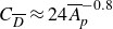 $C_{\overline{D}}\approx 24\overline{A}_{\!p}^{-0.8}$
. In fact, both oblate and prolate spheroidal grains are special cases of triaxial-ellipsoidal grains. Compared to one-angle-dependent
$C_{\overline{D}}\approx 24\overline{A}_{\!p}^{-0.8}$
. In fact, both oblate and prolate spheroidal grains are special cases of triaxial-ellipsoidal grains. Compared to one-angle-dependent $C_{\overline{D}}(\Theta )$
of spheroidal grains, the drag coefficient
$C_{\overline{D}}(\Theta )$
of spheroidal grains, the drag coefficient $C_{\overline{D}}(\Theta ,\Phi )$
of triaxial-ellipsoidal grains is two-angle-dependent. Albeit such a big difference,
$C_{\overline{D}}(\Theta ,\Phi )$
of triaxial-ellipsoidal grains is two-angle-dependent. Albeit such a big difference, $C_{\overline{D}}\propto \overline{A}_{\!p}^{-0.8}$
is also the case. For the better flow of logic, we put the derivation process in Appendix C.
$C_{\overline{D}}\propto \overline{A}_{\!p}^{-0.8}$
is also the case. For the better flow of logic, we put the derivation process in Appendix C.
The derived power law $C_{\overline{D}}\propto \overline{A}_{\!p}^{-0.8}$
is validated in figure 2 by the theoretical data points of both spheroidal and ellipsoidal grains. The more the grain shape departs from a perfect sphere, the more its data deviate from
$C_{\overline{D}}\propto \overline{A}_{\!p}^{-0.8}$
is validated in figure 2 by the theoretical data points of both spheroidal and ellipsoidal grains. The more the grain shape departs from a perfect sphere, the more its data deviate from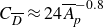 $C_{\overline{D}}\approx 24\overline{A}_{\!p}^{-0.8}$
; however, even when the short axis length is only half of that of the long axis for spheroidal grains,
$C_{\overline{D}}\approx 24\overline{A}_{\!p}^{-0.8}$
; however, even when the short axis length is only half of that of the long axis for spheroidal grains, $C_{\overline{D}}$
can be well linear to
$C_{\overline{D}}$
can be well linear to $\overline{A}_{\!p}^{-0.8}$
on a log-log scale. For brevity, we use only one parameter,
$\overline{A}_{\!p}^{-0.8}$
on a log-log scale. For brevity, we use only one parameter, $\varepsilon$
, to define the triaxial-ellipsoidal surface
$\varepsilon$
, to define the triaxial-ellipsoidal surface ${x^{2}}/{a^{2}}+{y^{2}}/({a^{2}(1-\varepsilon))}+{z^{2}}/({a^{2}(1-\varepsilon)^{2})}=1$
in figure 2(b). The data appear to be logarithmically linear for lower
${x^{2}}/{a^{2}}+{y^{2}}/({a^{2}(1-\varepsilon))}+{z^{2}}/({a^{2}(1-\varepsilon)^{2})}=1$
in figure 2(b). The data appear to be logarithmically linear for lower $\varepsilon$
. Interestingly, the relation between
$\varepsilon$
. Interestingly, the relation between $C_{\overline{D}}$
and
$C_{\overline{D}}$
and $\overline{A}_{\!p}$
becomes gradually not injective with increasing
$\overline{A}_{\!p}$
becomes gradually not injective with increasing $\varepsilon$
, as illustrated in the left-hand inset of figure 2(b). Albeit the emerging
$\varepsilon$
, as illustrated in the left-hand inset of figure 2(b). Albeit the emerging $(C_{\overline{D}},\overline{A}_{\!p})$
data form a scattered band rather than a clear line, the
$(C_{\overline{D}},\overline{A}_{\!p})$
data form a scattered band rather than a clear line, the $C_{\overline{D}}$
–
$C_{\overline{D}}$
– $\overline{A}_{\!p}$
relation can be well approximated by a log-linear function. Motivated by the high efficiency of this power law in ellipsoidal grains, we use obtained DNS results to examine whether this power law is suitable for rough grains, for which it is challenging to derive
$\overline{A}_{\!p}$
relation can be well approximated by a log-linear function. Motivated by the high efficiency of this power law in ellipsoidal grains, we use obtained DNS results to examine whether this power law is suitable for rough grains, for which it is challenging to derive $C_{\overline{D}}$
.
$C_{\overline{D}}$
.
Analytical results of $C_{\overline{D}}$
versus
$C_{\overline{D}}$
versus $\overline{A}_{\!p}$
for (a) spheroidal and (b) ellipsoidal grains. The black stars represent the sphere data. The colour bar is shared by both
$\overline{A}_{\!p}$
for (a) spheroidal and (b) ellipsoidal grains. The black stars represent the sphere data. The colour bar is shared by both $\epsilon \in [-0.5,0.5]$
and
$\epsilon \in [-0.5,0.5]$
and $\varepsilon \in [0.5,1]$
. The solid line denotes the fitting line via the formula
$\varepsilon \in [0.5,1]$
. The solid line denotes the fitting line via the formula $C_{\overline{D}}\propto \overline{A}_{\!p}^{-0.8}$
. Zoom-ins in all plots are for enlargements around the point
$C_{\overline{D}}\propto \overline{A}_{\!p}^{-0.8}$
. Zoom-ins in all plots are for enlargements around the point $(\overline{A}_{\!p},C_{\overline{D}})=(1,24)$
. In (a), the left bottom inset with
$(\overline{A}_{\!p},C_{\overline{D}})=(1,24)$
. In (a), the left bottom inset with $0\lt \epsilon \lt 0.5$
is for oblate spheroids marked by the square, while the right upper inset with
$0\lt \epsilon \lt 0.5$
is for oblate spheroids marked by the square, while the right upper inset with $-0.5\lt \epsilon \lt 0$
is for prolate spheroids marked by the circle.
$-0.5\lt \epsilon \lt 0$
is for prolate spheroids marked by the circle.

3.2. Universality of
$C_{\overline{D}}\propto \overline{A}_{\!p}^{-0.8}$

Mutual verifications between the derived power law $C_{\overline{D}}\propto \overline{A}_{\!p}^{-0.8}$
and DNS are demonstrated in figure 3(a), for which the fitting parameters are listed in Appendix D. The database contains one spherical, six oblate and five prolate spheroidal, and four triaxial-ellipsoidal grains, of which shape indices are summarized in table 8. The aspect ratio
$C_{\overline{D}}\propto \overline{A}_{\!p}^{-0.8}$
and DNS are demonstrated in figure 3(a), for which the fitting parameters are listed in Appendix D. The database contains one spherical, six oblate and five prolate spheroidal, and four triaxial-ellipsoidal grains, of which shape indices are summarized in table 8. The aspect ratio $\mathcal{A}_{\mathcal{R}}$
, defined as the ratio of the minimum to maximum radial length (see Appendix A), of oblate spheroids is
$\mathcal{A}_{\mathcal{R}}$
, defined as the ratio of the minimum to maximum radial length (see Appendix A), of oblate spheroids is $[0.1,0.9]$
, while the range of prolate spheroids is
$[0.1,0.9]$
, while the range of prolate spheroids is $[0.59,0.91]$
. Four triaxial ellipsoids are with the same
$[0.59,0.91]$
. Four triaxial ellipsoids are with the same $\mathcal{A}_{\mathscr{r}}$
, defined as the minimum to the maximum principal dimension in range
$\mathcal{A}_{\mathscr{r}}$
, defined as the minimum to the maximum principal dimension in range $[0.51,0.97]$
, for the rough particles
$[0.51,0.97]$
, for the rough particles $(R_{r},D_{\!f})\in \{(0.2,2.2),(0.2,2.5),(0.35,2.1),(0.35,2.5)\}$
. All ellipsoidal grains show good alignment with the line
$(R_{r},D_{\!f})\in \{(0.2,2.2),(0.2,2.5),(0.35,2.1),(0.35,2.5)\}$
. All ellipsoidal grains show good alignment with the line $C_{\overline{D}}=24\overline{A}_{\!p}^{-0.8}$
.
$C_{\overline{D}}=24\overline{A}_{\!p}^{-0.8}$
.
Log-log plots of $C_{\overline{D}}$
versus
$C_{\overline{D}}$
versus $\overline{A}_{\!p}$
for (a) the spherical, spheroidal and triaxial-ellipsoidal cases and (b–f) each
$\overline{A}_{\!p}$
for (a) the spherical, spheroidal and triaxial-ellipsoidal cases and (b–f) each $R_{r}$
. The dashed lines represent the fitting results using
$R_{r}$
. The dashed lines represent the fitting results using $C_{\overline{D}}\propto \overline{A}_{\!p}^{-0.8}$
. All fittings in (b–f) have R-squared values larger than 0.90, which are summarised in table 11 of Appendix D. The colour bar is shared by
$C_{\overline{D}}\propto \overline{A}_{\!p}^{-0.8}$
. All fittings in (b–f) have R-squared values larger than 0.90, which are summarised in table 11 of Appendix D. The colour bar is shared by $\epsilon \in [-0.7,0.9]$
,
$\epsilon \in [-0.7,0.9]$
, $\mathcal{A}_{\mathcal{R}}\in [0.5,0.8]$
and
$\mathcal{A}_{\mathcal{R}}\in [0.5,0.8]$
and $D_{\!f}\in [2.1,2.5]$
. The black star marks the value of a sphere. The
$D_{\!f}\in [2.1,2.5]$
. The black star marks the value of a sphere. The $x$
-axis range in all plots is
$x$
-axis range in all plots is $[0.9\min _{} \overline{A}_{\!p},1.1\max _{} \overline{A}_{\!p}]$
. Zoom-ins in all plots are for enlargements around the point
$[0.9\min _{} \overline{A}_{\!p},1.1\max _{} \overline{A}_{\!p}]$
. Zoom-ins in all plots are for enlargements around the point $(\overline{A}_{\!p},C_{\overline{D}})=(1,24)$
.
$(\overline{A}_{\!p},C_{\overline{D}})=(1,24)$
.

(a) Comparisons of $C_{\overline{D}}$
and (b) the ratio of pressure drag to friction drag between DNS results and the deterministic model from Leith (Reference Leith1987). In both plots, dashed lines represent the equality
$C_{\overline{D}}$
and (b) the ratio of pressure drag to friction drag between DNS results and the deterministic model from Leith (Reference Leith1987). In both plots, dashed lines represent the equality $y=x$
. Solid markers denote cases where the flow is perpendicular to the projected area in the plane spanned by
$y=x$
. Solid markers denote cases where the flow is perpendicular to the projected area in the plane spanned by $\boldsymbol{p}_{{1}}$
–
$\boldsymbol{p}_{{1}}$
– $\boldsymbol{p}_{{2}}$
or
$\boldsymbol{p}_{{2}}$
or $\boldsymbol{p}_{{2}}$
–
$\boldsymbol{p}_{{2}}$
– $\boldsymbol{p}_{{3}}$
. The red star is for the spherical case. Zoom-ins in all plots are for enlargements around the data point for the spherical case.
$\boldsymbol{p}_{{3}}$
. The red star is for the spherical case. Zoom-ins in all plots are for enlargements around the data point for the spherical case.

In line with testing whether analytics from minimal geometries apply to more complex shapes, the model of Leith (Reference Leith1987) may be the most accepted. Therein, it is postulated that since for a sphere in the Stokesian regime, two-thirds of the drag is due to viscous effects and one-third to the pressure drag, the same should hold for aspherical objects. With further consideration of $F_{\!D}$
as the integrations of fluid pressure and friction over the object surface, the former and the latter should be associated with the area projected normal to the fluid motion and the area of the total surface, respectively:
$F_{\!D}$
as the integrations of fluid pressure and friction over the object surface, the former and the latter should be associated with the area projected normal to the fluid motion and the area of the total surface, respectively:
 \begin{equation}F_{\!D}=6\pi \mu \left| \boldsymbol{u}_{\infty }\right| \left(\underset{\text{pressure}}{\underbrace{\frac{1}{3}R_{{A_{\!p}}}}}+\underset{\text{viscosity}}{\underbrace{\frac{2}{3}R_{{S_{a}}}}}\right)\!,\end{equation}
where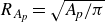 $R_{{A_{\!p}}}=\sqrt{{A_{\!p}}/{\pi }}$
and
$R_{{A_{\!p}}}=\sqrt{{A_{\!p}}/{\pi }}$
and $R_{{S_{a}}}=\sqrt{({S_{a}}/{4\pi }})$
are, respectively the radius lengths of the projected and surface-area-equivalent spheres. Importing this equation to measure the drag coefficient, we get
$R_{{S_{a}}}=\sqrt{({S_{a}}/{4\pi }})$
are, respectively the radius lengths of the projected and surface-area-equivalent spheres. Importing this equation to measure the drag coefficient, we get
 \begin{equation}C_{\!D}=\dfrac{24\pi \left(\dfrac{1}{3}R_{{A_{\!p}}}+\dfrac{2}{3}R_{{S_{a}}}\right)R_{\textit{eq}}}{Re\,A_{\!p}}\quad\rightarrow\quad C_{\overline{D}}=\frac{\left(8R_{{A_{\!p}}}+16R_{{S_{a}}}\right)R_{\textit{eq}}}{R_{{A_{\!p}}}^{2}},\end{equation}
and the ratio of pressure to friction drag is $R_{A_{p}}/(2R_{S_a})$
. Interestingly, as demonstrated in figure 4(a), except for the spherical case, results predicted by Leith’s model systematically depart from those from the DNS; this is because the pressure– and friction–drag contributions are nearly independent, as shown in figure 4(b). The ratio of the two departs well from the postulated value
$R_{A_{p}}/(2R_{S_a})$
. Interestingly, as demonstrated in figure 4(a), except for the spherical case, results predicted by Leith’s model systematically depart from those from the DNS; this is because the pressure– and friction–drag contributions are nearly independent, as shown in figure 4(b). The ratio of the two departs well from the postulated value ${R_{{A_{\!p}}}}/({2R_{{S_{a}}}})$
. It is worth noting that to further improve the accuracy of Leith’s model in predicting
${R_{{A_{\!p}}}}/({2R_{{S_{a}}}})$
. It is worth noting that to further improve the accuracy of Leith’s model in predicting $C_{\overline{D}}$
of realistic shaped grains, Hölzer & Sommerfeld (Reference Hughes and Mallet2008) utilised the lengthwise sphericity instead of the crosswise sphericity in the original model to account for the pressure part in total drag. Compared with the latter, the former is more complicated and involves in quantifying the average cross-sectional area parallel to the flow direction. This replacement can only slightly improve the predictive accuracy in the rough drag, as demonstrated in figure 10(a) of Appendix E for the roughest grain
$C_{\overline{D}}$
of realistic shaped grains, Hölzer & Sommerfeld (Reference Hughes and Mallet2008) utilised the lengthwise sphericity instead of the crosswise sphericity in the original model to account for the pressure part in total drag. Compared with the latter, the former is more complicated and involves in quantifying the average cross-sectional area parallel to the flow direction. This replacement can only slightly improve the predictive accuracy in the rough drag, as demonstrated in figure 10(a) of Appendix E for the roughest grain $(R_{r}=0.35,\ D_{\!f}=2.5)$
; it is less robust when compared with
$(R_{r}=0.35,\ D_{\!f}=2.5)$
; it is less robust when compared with $C_{\overline{D}}\propto \overline{A}_{\!p}^{-0.8}$
. This indicates the unreasonableness of directly splitting the overall drag by the fashion of Stokes’ law, when coping with the interaction between a rough grain and the fluid around it.
$C_{\overline{D}}\propto \overline{A}_{\!p}^{-0.8}$
. This indicates the unreasonableness of directly splitting the overall drag by the fashion of Stokes’ law, when coping with the interaction between a rough grain and the fluid around it.
Then we further test our power law $C_{\overline{D}}\propto \overline{A}_{\!p}^{-0.8}$
against the asymmetrical rough grains. From figures 3(b–f), it can be seen that when
$C_{\overline{D}}\propto \overline{A}_{\!p}^{-0.8}$
against the asymmetrical rough grains. From figures 3(b–f), it can be seen that when $\overline{A}_{\!p}$
values are within
$\overline{A}_{\!p}$
values are within $[0.9,1.8]$
for all rough grains shown in figure 1(a), the power law still holds. However, the scale factor
$[0.9,1.8]$
for all rough grains shown in figure 1(a), the power law still holds. However, the scale factor $a$
in
$a$
in $C_{\overline{D}}=a\overline{A}_{\!p}^{-0.8}$
is no longer 24, and depends on the grain morphology (see table 10 in Appendix D). Generally, the rougher a grain is, the smaller the scale factor may become, though it is not strictly monotonic with
$C_{\overline{D}}=a\overline{A}_{\!p}^{-0.8}$
is no longer 24, and depends on the grain morphology (see table 10 in Appendix D). Generally, the rougher a grain is, the smaller the scale factor may become, though it is not strictly monotonic with $R_{r}$
or
$R_{r}$
or $D_{\!f}$
, and the smallest
$D_{\!f}$
, and the smallest $a$
appears at
$a$
appears at $R_{r}=0.20,\ D_{\!f}=2.5$
. More importantly, for each rough grain considered, most orientations result in
$R_{r}=0.20,\ D_{\!f}=2.5$
. More importantly, for each rough grain considered, most orientations result in $C_{\overline{D}}$
values lower than that of the spherical case, indicating a net drag reduction, as shown in figures 3(b–f). Roughness causes concave surficial features, which are in nature different from purely convex geometries, such as ellipsoids. It apparently leads to two factors contributing to this drag reduction according to
$C_{\overline{D}}$
values lower than that of the spherical case, indicating a net drag reduction, as shown in figures 3(b–f). Roughness causes concave surficial features, which are in nature different from purely convex geometries, such as ellipsoids. It apparently leads to two factors contributing to this drag reduction according to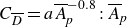 $C_{\overline{D}}=a\overline{A}_{\!p}^{-0.8} : \overline{A}_{\!p}$
is mostly smaller than 1, and
$C_{\overline{D}}=a\overline{A}_{\!p}^{-0.8} : \overline{A}_{\!p}$
is mostly smaller than 1, and $a$
is smaller than 24. In the following sections, after discussing which is the dominant role between pressure and friction drag in drag reduction, more evidence from micromechanical analysis will be provided.
$a$
is smaller than 24. In the following sections, after discussing which is the dominant role between pressure and friction drag in drag reduction, more evidence from micromechanical analysis will be provided.
Taken together, the simulations calibrate the 0.8 power law over a finite morphological and geometrical range. For the considered ellipsoids, the aspect ratio $\mathcal{A}_{\mathcal{R}}$
(defined as the ratio of minimum to maximum radial length; see Appendix A) spans
$\mathcal{A}_{\mathcal{R}}$
(defined as the ratio of minimum to maximum radial length; see Appendix A) spans $[0.1,0.9]$
for oblate spheroids, and
$[0.1,0.9]$
for oblate spheroids, and $[0.59,0.91]$
for prolate spheroids, and the PCA-determined equivalent-ellipsoid aspect ratio
$[0.59,0.91]$
for prolate spheroids, and the PCA-determined equivalent-ellipsoid aspect ratio $\mathcal{A}_{\mathscr{r}}$
of triaxial ellipsoids lies in
$\mathcal{A}_{\mathscr{r}}$
of triaxial ellipsoids lies in $[0.51,0.97]$
. The rough grains span
$[0.51,0.97]$
. The rough grains span $R_{r}\in [0.01,0.35]$
and
$R_{r}\in [0.01,0.35]$
and $D_{\!f}\in [2.1,2.5]$
. For all these shapes with various orientations such that
$D_{\!f}\in [2.1,2.5]$
. For all these shapes with various orientations such that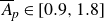 $\overline{A}_{\!p}\in [0.9,1.8]$
, the Reynolds-number-normalised drag coefficient can be well described by
$\overline{A}_{\!p}\in [0.9,1.8]$
, the Reynolds-number-normalised drag coefficient can be well described by $C_{\overline{D}}=\alpha \overline{A}_{\!p}^{-0.8}$
with R-squared values much higher than 0.9, as shown in figure 3 and Appendix D. Outside such an interval for
$C_{\overline{D}}=\alpha \overline{A}_{\!p}^{-0.8}$
with R-squared values much higher than 0.9, as shown in figure 3 and Appendix D. Outside such an interval for $\overline{A}_{\!p}$
, system deviations from the fit are encountered. Therefore, the scaling law should not be used for quantitative extrapolation there, such as the extremely high or low values of
$\overline{A}_{\!p}$
, system deviations from the fit are encountered. Therefore, the scaling law should not be used for quantitative extrapolation there, such as the extremely high or low values of $\overline{A}_{\!p}$
for an oblate spheroid with
$\overline{A}_{\!p}$
for an oblate spheroid with $\mathcal{A}_{\mathcal{R}}=0.1$
, as demonstrated in figure 3(a).
$\mathcal{A}_{\mathcal{R}}=0.1$
, as demonstrated in figure 3(a).
We have also benchmarked our 0.8 power law against representative classical drag correlations for non-spherical particles, summarised in table 12 in Appendix E. The main outcome is that the present projected-area-based closure remains competitive for axisymmetric bodies in the creeping-flow limit, and becomes particularly advantageous for two-angle-dependent grains, such as triaxial ellipsoids and rough grains. The detailed comparison is deferred to § 6.1, with the indicative proof in figure 10 in Appendix E.
Survival probability function $P_{s}$
of (a–e)
$P_{s}$
of (a–e) $C_{\overline{D}}$
, (f–j)
$C_{\overline{D}}$
, (f–j) ${C}_{\overline{D}}^{f}$
and (k–o)
${C}_{\overline{D}}^{f}$
and (k–o) ${C}_{\overline{D}}^{p}$
at varying rotation angles for each grain morphology in the
${C}_{\overline{D}}^{p}$
at varying rotation angles for each grain morphology in the $R_{r}$
–
$R_{r}$
– $D_{\!f}$
space. The columns from left to right correspond to
$D_{\!f}$
space. The columns from left to right correspond to $R_{r}$
values 0.01, 0.05, 0.10, 0.20 and 0.35. In each plot, the solid mark represents data of the flow perpendicular to the projected area on the plane crossed by
$R_{r}$
values 0.01, 0.05, 0.10, 0.20 and 0.35. In each plot, the solid mark represents data of the flow perpendicular to the projected area on the plane crossed by $\boldsymbol{p}_{{1}}$
and
$\boldsymbol{p}_{{1}}$
and $\boldsymbol{p}_{{2}}$
or
$\boldsymbol{p}_{{2}}$
or $\boldsymbol{p}_{{2}}$
and
$\boldsymbol{p}_{{2}}$
and $\boldsymbol{p}_{{3}}$
. The solid line represents the fitting using the survival probability function of the Weibull distribution. The dashed line denotes values of the spherical case.
$\boldsymbol{p}_{{3}}$
. The solid line represents the fitting using the survival probability function of the Weibull distribution. The dashed line denotes values of the spherical case.

4. Distributions of roughness-dependent
${C}_{\overline{{D}}}$
,
${{C}}_{\overline{{D}}}^{{f}}$
and
${{C}}_{\overline{{D}}}^{{p}}$


To examine grain morphology effects on the macroscopic drag, we compare in figures 5(a–e) distributions of $C_{\overline{D}}$
collected at varying rotation angles for different grain morphologies; the distribution is characterised by survival probability function
$C_{\overline{D}}$
collected at varying rotation angles for different grain morphologies; the distribution is characterised by survival probability function $P_{s}(C_{\overline{D}})=P(\tilde{C}_{\overline{D}}\gt C_{\overline{D}})=1-F(C_{\overline{D}})$
, where
$P_{s}(C_{\overline{D}})=P(\tilde{C}_{\overline{D}}\gt C_{\overline{D}})=1-F(C_{\overline{D}})$
, where $F(C_{\overline{D}})$
is the corresponding accumulative distribution function, and
$F(C_{\overline{D}})$
is the corresponding accumulative distribution function, and $\tilde{C}_{\overline{D}}$
is the stochastic value of the
$\tilde{C}_{\overline{D}}$
is the stochastic value of the $C_{\overline{D}}$
distribution. The drag coefficient is found to be strongly dependent on
$C_{\overline{D}}$
distribution. The drag coefficient is found to be strongly dependent on $R_{r}$
. When
$R_{r}$
. When $R_{r}$
is small, i.e. grains are closely spherical,
$R_{r}$
is small, i.e. grains are closely spherical, $C_{\overline{D}}$
spans a very narrow range around the value of the spherical case,
$C_{\overline{D}}$
spans a very narrow range around the value of the spherical case, $C_{\overline{D}0}$
, and is influenced little by
$C_{\overline{D}0}$
, and is influenced little by $D_{\!f}$
, suggesting that the drag of a small-
$D_{\!f}$
, suggesting that the drag of a small- $R_{r}$
grain can be approximated using
$R_{r}$
grain can be approximated using $C_{\overline{D}0}$
. When increasing
$C_{\overline{D}0}$
. When increasing $R_{r}$
, particles become more irregular, and the distribution of
$R_{r}$
, particles become more irregular, and the distribution of $C_{\overline{D}}$
widens and notably shifts towards smaller
$C_{\overline{D}}$
widens and notably shifts towards smaller $C_{\overline{D}}$
. This trend persists with higher
$C_{\overline{D}}$
. This trend persists with higher $D_{\!f}$
, especially for cases of larger
$D_{\!f}$
, especially for cases of larger $R_{r}$
. In essence, both
$R_{r}$
. In essence, both $R_{r}$
and
$R_{r}$
and $D_{\!f}$
result in the observed drag reduction, which is qualitatively consistent with some observations in rough–wall flows at high
$D_{\!f}$
result in the observed drag reduction, which is qualitatively consistent with some observations in rough–wall flows at high ${\textit{Re}}$
(Choi et al. Reference Chéron, Evrard and van Wachem2008), although the underlying physics differs from the single–grain Stokes problem considered here. Notably, a complete drag reduction, i.e.
${\textit{Re}}$
(Choi et al. Reference Chéron, Evrard and van Wachem2008), although the underlying physics differs from the single–grain Stokes problem considered here. Notably, a complete drag reduction, i.e. $C_{\overline{D}}\leq C_{\overline{D}0}$
, might be observed, if and only if both
$C_{\overline{D}}\leq C_{\overline{D}0}$
, might be observed, if and only if both $R_{r}$
and
$R_{r}$
and $D_{\!f}$
are of higher values, with the corresponding drag overestimated by Stokes’ formula.
$D_{\!f}$
are of higher values, with the corresponding drag overestimated by Stokes’ formula.
To quantitatively characterise the impacts of grain morphology, a statistical model is developed. Here, we find that distributions of $C_{\overline{D}}$
for a rough grain at various rotation angles follow a Weibull-like distribution, as the fitting using the Weibull distribution well matches the simulation results shown in figures 5(a–e). Additionally, we also calculate the lift coefficient
$C_{\overline{D}}$
for a rough grain at various rotation angles follow a Weibull-like distribution, as the fitting using the Weibull distribution well matches the simulation results shown in figures 5(a–e). Additionally, we also calculate the lift coefficient $C_{\overline{L}}={\textit{Re}}\,C_{L}$
and its two components, pressure part
$C_{\overline{L}}={\textit{Re}}\,C_{L}$
and its two components, pressure part ${C_{\overline{L}}}^{p}$
, and friction part
${C_{\overline{L}}}^{p}$
, and friction part ${C_{\overline{L}}}^{f}$
, from DNS, and find that for a rough grain, it follows a Weibull distribution as well (see Appendix F). Contrary to
${C_{\overline{L}}}^{f}$
, from DNS, and find that for a rough grain, it follows a Weibull distribution as well (see Appendix F). Contrary to $C_{\overline{D}}$
, with more severe global irregularity, quantified by higher values of
$C_{\overline{D}}$
, with more severe global irregularity, quantified by higher values of $R_{r}$
or
$R_{r}$
or $\mathcal{A}_{\mathscr{r}}$
, a net increase of
$\mathcal{A}_{\mathscr{r}}$
, a net increase of $C_{\overline{L}}$
is encountered, which is consistent with previous numerical studies on rotational-symmetrical grains (Zastawny et al. Reference Zastawny, Mallouppas, Zhao and van Wachem2012; van Wachem et al. Reference van Wachem, Zastawny, Zhao and Mallouppas2015; Ouchene et al. Reference Ouchene, Khalij, Arcen and Tanière2016; Chéron et al. Reference Choi, Jeon and Kim2024) and realistic-shaped grains (Sommerfeld & Qadir Reference Sommerfeld and Qadir2018; Castang et al. Reference Castang, Laín, García and Sommerfeld2022). Another obvious feature – which also occurs in figure 12 for
$C_{\overline{L}}$
is encountered, which is consistent with previous numerical studies on rotational-symmetrical grains (Zastawny et al. Reference Zastawny, Mallouppas, Zhao and van Wachem2012; van Wachem et al. Reference van Wachem, Zastawny, Zhao and Mallouppas2015; Ouchene et al. Reference Ouchene, Khalij, Arcen and Tanière2016; Chéron et al. Reference Choi, Jeon and Kim2024) and realistic-shaped grains (Sommerfeld & Qadir Reference Sommerfeld and Qadir2018; Castang et al. Reference Castang, Laín, García and Sommerfeld2022). Another obvious feature – which also occurs in figure 12 for $C_{\overline{L}}$
,
$C_{\overline{L}}$
, $C_{\overline{L}}^{f}$
and
$C_{\overline{L}}^{f}$
and $C_{\overline{L}}^{p}$
– is the shrinkage of
$C_{\overline{L}}^{p}$
– is the shrinkage of $C_{\!D}$
,
$C_{\!D}$
, $C_{\overline{D}}^{f}$
and
$C_{\overline{D}}^{f}$
and $C_{\overline{D}}^{p}$
with higher
$C_{\overline{D}}^{p}$
with higher $D_{\!f}$
values of the same
$D_{\!f}$
values of the same $R_{r}$
. This can be explained in two ways: (i) higher
$R_{r}$
. This can be explained in two ways: (i) higher $D_{\!f}$
might introduce a narrow range of
$D_{\!f}$
might introduce a narrow range of $A_{\!p}$
that has a larger net value than those of lower
$A_{\!p}$
that has a larger net value than those of lower $D_{\!f}$
; and (ii) more locally isotropic morphology without obvious orientations could be depicted, and the associated local fluid–grain interaction forces become more isotropic and generate lower interaction force on the grain surface.
$D_{\!f}$
; and (ii) more locally isotropic morphology without obvious orientations could be depicted, and the associated local fluid–grain interaction forces become more isotropic and generate lower interaction force on the grain surface.
Why is the Weibullian behaviour encountered in the distribution of $C_{\overline{D}}$
for various rough grains? To answer this question, we look back at its power-law dependence on
$C_{\overline{D}}$
for various rough grains? To answer this question, we look back at its power-law dependence on $\overline{A}_{\!p} : C_{\overline{D}}=a\overline{A}_{\!p}^{-0.8}$
; i.e.
$\overline{A}_{\!p} : C_{\overline{D}}=a\overline{A}_{\!p}^{-0.8}$
; i.e. $C_{\overline{D}}$
conforms to a Weibull distribution if
$C_{\overline{D}}$
conforms to a Weibull distribution if $\overline{A}_{\!p}$
conforms to a Weibull distribution, for which the survival probability function
$\overline{A}_{\!p}$
conforms to a Weibull distribution, for which the survival probability function $P_{s}(\overline{A}_{\!p})$
reads
$P_{s}(\overline{A}_{\!p})$
reads
 \begin{equation}P_{s}\left(\overline{A}_{\!p}\right)=\text{e}^{{-\left(\overline{A}_{\!p}/\lambda _{\!p}\right)^{{k_{\!p}}}}},\end{equation}
where $\lambda _{\!p}$
is the scale parameter with
$\lambda _{\!p}$
is the scale parameter with $P_{s}(\lambda _{\!p})={\rm e}^{-1}\approx 36.79\,\%$
, and
$P_{s}(\lambda _{\!p})={\rm e}^{-1}\approx 36.79\,\%$
, and $k_{\!p}$
is the shape parameter that determines the stretch of
$k_{\!p}$
is the shape parameter that determines the stretch of $P_{s}(\overline{A}_{\!p})$
. Then the distribution of
$P_{s}(\overline{A}_{\!p})$
. Then the distribution of $C_{\overline{D}}$
can be derived as
$C_{\overline{D}}$
can be derived as
 \begin{equation}P_{s}\left(C_{\overline{D}}\right)=1-{\rm e}^{{-\left(\frac{C_{\overline{D}}}{a{\lambda }_{\!p}^{-0.8}}\right)^{-{k_{\!p}}/0.8}}}.\end{equation}
One can see that $P_{s}(C_{\overline{D}})$
is in a form that is similar to the Weibullian scheme but not strictly the same since the shape parameter is negative. Because of the negative exponent,
$P_{s}(C_{\overline{D}})$
is in a form that is similar to the Weibullian scheme but not strictly the same since the shape parameter is negative. Because of the negative exponent, $P_{s}(C_{\overline{D}})$
exhibits a Fréchet-type heavy tail rather than a Weibull tail. This helps to explain why
$P_{s}(C_{\overline{D}})$
exhibits a Fréchet-type heavy tail rather than a Weibull tail. This helps to explain why $C_{\overline{D}}$
conforms to a Weibull-like distribution with
$C_{\overline{D}}$
conforms to a Weibull-like distribution with $C_{\overline{D}}\propto \overline{A}_{\!p}^{-0.8}$
for a rough grain with certain
$C_{\overline{D}}\propto \overline{A}_{\!p}^{-0.8}$
for a rough grain with certain $R_{r}$
and
$R_{r}$
and $D_{\!f}$
.
$D_{\!f}$
.
Both the assumption of $\overline{A}_{\!p}$
and the derivation of
$\overline{A}_{\!p}$
and the derivation of $P_{s}(C_{\overline{D}})$
are tested. First, Kljuno & Catovic (Reference Kljuno and Catovic2019) demonstrated that the projected area of an irregularly shaped grain could be accurately estimated by that of its equivalent triaxial ellipsoid. We prove in Appendix G that the distribution of
$P_{s}(C_{\overline{D}})$
are tested. First, Kljuno & Catovic (Reference Kljuno and Catovic2019) demonstrated that the projected area of an irregularly shaped grain could be accurately estimated by that of its equivalent triaxial ellipsoid. We prove in Appendix G that the distribution of $\overline{A}_{\!p}$
of ellipsoidal grains can be well approximated by the Weibull distribution. More directly, figures 6(a–e) show the distribution of
$\overline{A}_{\!p}$
of ellipsoidal grains can be well approximated by the Weibull distribution. More directly, figures 6(a–e) show the distribution of $\overline{A}_{\!p}$
for each rough grain. Although a two-parameter Weibull fit captures the bulk of the distribution (approximately at
$\overline{A}_{\!p}$
for each rough grain. Although a two-parameter Weibull fit captures the bulk of the distribution (approximately at $10\,\% \lt P_{s}\lt 90\,\%$
), systematic deviations appear near the lower bound of
$10\,\% \lt P_{s}\lt 90\,\%$
), systematic deviations appear near the lower bound of $\overline{A}_{\!p}$
for each case. This is expected because
$\overline{A}_{\!p}$
for each case. This is expected because $\overline{A}_{\!p}$
has a finite support
$\overline{A}_{\!p}$
has a finite support $[\overline{A}_{p, \textit{min}},\overline{A}_{p, \textit{max}}]$
, whereas the two-parameter Weibull assumes support on
$[\overline{A}_{p, \textit{min}},\overline{A}_{p, \textit{max}}]$
, whereas the two-parameter Weibull assumes support on $[0,\infty )$
. The values of
$[0,\infty )$
. The values of $\lambda _{\!p}$
and
$\lambda _{\!p}$
and $k_{\!p}$
can be found in tables 13 and 14 of Appendix H. Using the inverse power law mapping
$k_{\!p}$
can be found in tables 13 and 14 of Appendix H. Using the inverse power law mapping $C_{\overline{D}}=a\overline{A}_{\!p}^{-0.8}$
, (4.2) transforms the Weibull-like
$C_{\overline{D}}=a\overline{A}_{\!p}^{-0.8}$
, (4.2) transforms the Weibull-like $\overline{A}_{\!p}$
fit into a Fréchet-type survival function for
$\overline{A}_{\!p}$
fit into a Fréchet-type survival function for $C_{\overline{D}}$
. As a result, small misfits near
$C_{\overline{D}}$
. As a result, small misfits near $\overline{A}_{p, \textit{min}}$
are amplified into the upper tail of
$\overline{A}_{p, \textit{min}}$
are amplified into the upper tail of $P_{s}(C_{\overline{D}})$
. The predictions therefore reproduce the central probability mass of the distributions, but underestimate the upper tail in figures 6(f–j), most notably for higher
$P_{s}(C_{\overline{D}})$
. The predictions therefore reproduce the central probability mass of the distributions, but underestimate the upper tail in figures 6(f–j), most notably for higher $R_{r}$
.
$R_{r}$
.
The grain drag force arises from the combined effects of skin friction ${C}_{\overline{D}}^{f}$
and pressure drag
${C}_{\overline{D}}^{f}$
and pressure drag ${C}_{\overline{D}}^{p}$
. Interestingly, figure 5 shows that both
${C}_{\overline{D}}^{p}$
. Interestingly, figure 5 shows that both ${C}_{\overline{D}}^{f}$
and
${C}_{\overline{D}}^{f}$
and ${C}_{\overline{D}}^{p}$
also follow Weibull distributions, regardless of
${C}_{\overline{D}}^{p}$
also follow Weibull distributions, regardless of $R_{r}$
and
$R_{r}$
and $D_{\!f}$
. Figures 5(f–j) suggest that
$D_{\!f}$
. Figures 5(f–j) suggest that ${C}_{\overline{D}}^{f}$
follows a similar trend to
${C}_{\overline{D}}^{f}$
follows a similar trend to $C_{\overline{D}}$
. However,
$C_{\overline{D}}$
. However, ${C}_{\overline{D}}^{p}$
shows little sensitivity to grain morphology, especially to
${C}_{\overline{D}}^{p}$
shows little sensitivity to grain morphology, especially to $D_{\!f}$
. As illustrated in figures 5(k–o), all results with the same
$D_{\!f}$
. As illustrated in figures 5(k–o), all results with the same $R_{r}$
but different
$R_{r}$
but different $D_{\!f}$
are almost collapsed on the same line. In particular, the mean value of
$D_{\!f}$
are almost collapsed on the same line. In particular, the mean value of ${C}_{\overline{D}}^{p}$
is close to
${C}_{\overline{D}}^{p}$
is close to ${C}_{\overline{D}0}^{p}$
for the spherical case with a relatively small deviation. Therefore, it can be concluded that the drag reduction is mainly attributed to the decrease in skin friction, whilst the pressure drag exerts a limited influence. All these macro observations necessitate a detailed documentation of microfluid mechanics for potential explanations.
${C}_{\overline{D}0}^{p}$
for the spherical case with a relatively small deviation. Therefore, it can be concluded that the drag reduction is mainly attributed to the decrease in skin friction, whilst the pressure drag exerts a limited influence. All these macro observations necessitate a detailed documentation of microfluid mechanics for potential explanations.
Survival probability function $P_{s}$
of (a–e)
$P_{s}$
of (a–e) $\overline{A}_{\!p}$
and (f–j)
$\overline{A}_{\!p}$
and (f–j) $C_{\overline{D}}$
with corresponding fitting lines. The colours and symbols represent different
$C_{\overline{D}}$
with corresponding fitting lines. The colours and symbols represent different $D_{\!f}$
and
$D_{\!f}$
and $R_{r}$
following the same scheme as figure 4. The solid line represents the fitting using the survival probability function of the Weibull distribution. The dashed line denotes values of the spherical case.
$R_{r}$
following the same scheme as figure 4. The solid line represents the fitting using the survival probability function of the Weibull distribution. The dashed line denotes values of the spherical case.

5. Roughness-scale micromechanics of pressure and friction drag
To elucidate the underlying roughness-scale mechanisms, we first provide distributions of friction ${\tau _{x}}=\boldsymbol{\tau }\boldsymbol{\cdot }\boldsymbol{n}_{x}$
and pressure
${\tau _{x}}=\boldsymbol{\tau }\boldsymbol{\cdot }\boldsymbol{n}_{x}$
and pressure $p_{x}=p\boldsymbol{I}\boldsymbol{\cdot }\boldsymbol{n}_{x}$
stresses on grain surfaces at a specific set of rotation angles. For each morphology in figure 1(a), we select the rotation yielding
$p_{x}=p\boldsymbol{I}\boldsymbol{\cdot }\boldsymbol{n}_{x}$
stresses on grain surfaces at a specific set of rotation angles. For each morphology in figure 1(a), we select the rotation yielding $C_{\overline{D}}$
closest to the mean value. As in figure 7, with a sphere as the reference (Happel & Brenner Reference Happel and Brenner1983),
$C_{\overline{D}}$
closest to the mean value. As in figure 7, with a sphere as the reference (Happel & Brenner Reference Happel and Brenner1983),
 \begin{align} \tau _{x,s}&=3U_{{\infty }}\mu _{\!f}d_{\textit{eq}}\sin ^{2} \vartheta, \end{align}
 \begin{align} p_{x,s}&=3U_{{\infty }}\mu _{\!f}d_{\textit{eq}}\cos ^{2} \vartheta, \end{align}
where $\vartheta$
is the angle between the vector connecting the grain centre and surficial point and the counter-direction vector of flow, as depicted in figure 1(b), and
$\vartheta$
is the angle between the vector connecting the grain centre and surficial point and the counter-direction vector of flow, as depicted in figure 1(b), and $\tau _{x,s}$
and
$\tau _{x,s}$
and $p_{x,s}$
are friction and pressure components of drag pressure on a sphere, respectively. Here,
$p_{x,s}$
are friction and pressure components of drag pressure on a sphere, respectively. Here, $\tau _{x}$
exhibits a belted distribution with intense values around the equator, and relatively weaker values at the front and back polar areas. Such a distribution persists when
$\tau _{x}$
exhibits a belted distribution with intense values around the equator, and relatively weaker values at the front and back polar areas. Such a distribution persists when $R_{r}$
and
$R_{r}$
and $D_{\!f}$
are small. On rougher grains, though this global characteristic never vanishes due to the nature of shear flows, a significant localisation is observed, i.e. distributions of
$D_{\!f}$
are small. On rougher grains, though this global characteristic never vanishes due to the nature of shear flows, a significant localisation is observed, i.e. distributions of $\tau _{x}$
become more reliant on local geometric features. Specifically,
$\tau _{x}$
become more reliant on local geometric features. Specifically, $\tau _{x}$
is intense at ridges while weak at dimples. On the contrary,
$\tau _{x}$
is intense at ridges while weak at dimples. On the contrary, $p_{x}$
on irregularly shaped grains approximately retains the shape of
$p_{x}$
on irregularly shaped grains approximately retains the shape of $p_{x,s}$
on the smoothed sphere.
$p_{x,s}$
on the smoothed sphere.
The distribution of (a) streamwise shear stress $\boldsymbol{\tau }\boldsymbol{\cdot }\boldsymbol{n}_{x}$
and (b) pressure
$\boldsymbol{\tau }\boldsymbol{\cdot }\boldsymbol{n}_{x}$
and (b) pressure $p$
on a sphere, and (c)
$p$
on a sphere, and (c) $\boldsymbol{\tau }\boldsymbol{\cdot }\boldsymbol{n}_{x}$
and (d)
$\boldsymbol{\tau }\boldsymbol{\cdot }\boldsymbol{n}_{x}$
and (d) $p$
on rough grains. (e) The distribution of streamlines and shear rate for the case with
$p$
on rough grains. (e) The distribution of streamlines and shear rate for the case with $D_{\!f}=2.4$
and
$D_{\!f}=2.4$
and $R_{r}=0.1$
and its zoomed-in
$R_{r}=0.1$
and its zoomed-in $x$
–
$x$
– $y$
plane.
$y$
plane.

The observed difference in stress distribution between the spherical and rough grains can be explained by figure 7(e), demonstrating the streamlines around the rough grain. First, ridges and dimples are identified using a convex hull, where vertices indicate the ridges and dimples located between them. Since it is submerged in an open domain, recirculation is not observed in the conducted simulations with low ${\textit{Re}}$
. However, distinct shear rates are encountered near ridge and dimple regions, as indicated by the zoom-in of figure 7(e), due to the flow deceleration at dimples and acceleration at ridges. Consequently, the skin friction is enhanced at ridges while weakened at dimples. These competing effects collectively determine the overall drag. Notably, the influenced areas differ between dimples and ridges. A ridge appears as a wall-mounted singularity, and only influences a narrow surrounding area, whereas a dimple covers a wider area where
${\textit{Re}}$
. However, distinct shear rates are encountered near ridge and dimple regions, as indicated by the zoom-in of figure 7(e), due to the flow deceleration at dimples and acceleration at ridges. Consequently, the skin friction is enhanced at ridges while weakened at dimples. These competing effects collectively determine the overall drag. Notably, the influenced areas differ between dimples and ridges. A ridge appears as a wall-mounted singularity, and only influences a narrow surrounding area, whereas a dimple covers a wider area where $\boldsymbol{\tau }\boldsymbol{\cdot }\boldsymbol{n}_{x}$
is effectively mitigated. Compared with
$\boldsymbol{\tau }\boldsymbol{\cdot }\boldsymbol{n}_{x}$
is effectively mitigated. Compared with $D_{\!f}$
controlling the local features of a grain without changing the general shapes, higher
$D_{\!f}$
controlling the local features of a grain without changing the general shapes, higher $R_{r}$
turns out to be more pronounced, leading to a significant drag reduction.
$R_{r}$
turns out to be more pronounced, leading to a significant drag reduction.
Cumulative distribution function $P_{c}$
of (a–e)
$P_{c}$
of (a–e) $\Delta \tau _{x}$
and (f–j)
$\Delta \tau _{x}$
and (f–j) $\Delta p_{x}$
, whose values are scaled by
$\Delta p_{x}$
, whose values are scaled by $3U_{{\infty }}\mu _{\!f}d_{\textit{eq}}$
, for each grain morphology in the
$3U_{{\infty }}\mu _{\!f}d_{\textit{eq}}$
, for each grain morphology in the $R_{r}$
–
$R_{r}$
– $D_{\!f}$
space. The columns from left to right correspond to
$D_{\!f}$
space. The columns from left to right correspond to $R_{r}$
values 0.01, 0.05, 0.10, 0.20 and 0.35. In each plot, the solid lines are normal distribution fitting results. The colours and symbols represent different
$R_{r}$
values 0.01, 0.05, 0.10, 0.20 and 0.35. In each plot, the solid lines are normal distribution fitting results. The colours and symbols represent different $D_{\!f}$
and
$D_{\!f}$
and $R_{r}$
following the same scheme as in figure 5. The horizontal dashed line in all plots represents
$R_{r}$
following the same scheme as in figure 5. The horizontal dashed line in all plots represents $P_{c}=50\,\%$
, while the vertical dashed line denotes
$P_{c}=50\,\%$
, while the vertical dashed line denotes $\Delta \tau _{x}=0$
in (a–e) and
$\Delta \tau _{x}=0$
in (a–e) and $\Delta p_{x}=0$
in (f–j).
$\Delta p_{x}=0$
in (f–j).

As to $p$
in figure 7(d), though the local extrema emerge due to the roughness, their distribution remains similar to that of a sphere in figure 7(b). Generally, the high pressure can be observed at the upstream surface, while the low pressure occurs at the downstream. The pressure drag is determined by the pressure difference between the upstream and downstream surfaces, which seems to be more dependent on the general grain shape than the local waviness.
$p$
in figure 7(d), though the local extrema emerge due to the roughness, their distribution remains similar to that of a sphere in figure 7(b). Generally, the high pressure can be observed at the upstream surface, while the low pressure occurs at the downstream. The pressure drag is determined by the pressure difference between the upstream and downstream surfaces, which seems to be more dependent on the general grain shape than the local waviness.
We conduct a stress analysis to further clarify the mechanism underpinning the drag reduction. Assume that the counterparts of a rough grain are functions of $\Theta$
and
$\Theta$
and $\Phi$
expressed in an incremental formation, i.e.
$\Phi$
expressed in an incremental formation, i.e.
 \begin{align} \tau _{x}(\vartheta )&=\tau _{x,s}(\vartheta )+\Delta \tau _{x}(\vartheta ),\end{align}
 \begin{align} p_{x}(\vartheta )&=p_{x,s}(\vartheta )+\Delta p_{x}(\vartheta ).\end{align}
Here, $\Delta \tau _{x}(\vartheta )$
and
$\Delta \tau _{x}(\vartheta )$
and $\Delta p_{x}(\vartheta )$
measure the contributions of roughness to the total drag, and the statistical distributions of each rough grain with all rotations are provided in figure 8, where results are scaled by
$\Delta p_{x}(\vartheta )$
measure the contributions of roughness to the total drag, and the statistical distributions of each rough grain with all rotations are provided in figure 8, where results are scaled by $3U_{{\infty }}\mu _{\!f}d_{\textit{eq}}$
. Both distributions of
$3U_{{\infty }}\mu _{\!f}d_{\textit{eq}}$
. Both distributions of $\Delta \tau _{x}(\vartheta )$
and
$\Delta \tau _{x}(\vartheta )$
and $\Delta p_{x}(\vartheta )$
follow a Gaussian pattern for all cases. Interestingly, the distribution of
$\Delta p_{x}(\vartheta )$
follow a Gaussian pattern for all cases. Interestingly, the distribution of $\Delta p_{x}$
is perfectly symmetric around
$\Delta p_{x}$
is perfectly symmetric around $\Delta p_{x}=0$
, i.e. its expectation is zero, suggesting that the net contribution of
$\Delta p_{x}=0$
, i.e. its expectation is zero, suggesting that the net contribution of $\Delta p_{x}$
to the total grain drag is almost zero, therefore explaining that the mean
$\Delta p_{x}$
to the total grain drag is almost zero, therefore explaining that the mean ${C}_{\overline{D}}^{p}$
is insensitive to the grain morphology shown in figures 5(k–o). Also, this symmetric distribution aligns with the observation in figure 7(d) where the distribution of
${C}_{\overline{D}}^{p}$
is insensitive to the grain morphology shown in figures 5(k–o). Also, this symmetric distribution aligns with the observation in figure 7(d) where the distribution of $p$
remains similar to that of the sphere. Different from
$p$
remains similar to that of the sphere. Different from $\Delta p_{x}$
, the distribution of
$\Delta p_{x}$
, the distribution of $\Delta \tau _{x}$
appears asymmetric. Its mean value shifts to the negative zone (
$\Delta \tau _{x}$
appears asymmetric. Its mean value shifts to the negative zone ( $\Delta \tau _{x}\lt 0$
), and the rougher the grain is, the more significant the shift becomes, suggesting that
$\Delta \tau _{x}\lt 0$
), and the rougher the grain is, the more significant the shift becomes, suggesting that $\Delta \tau _{x}$
mainly contributes to the drag reduction and confirming the conclusions drawn from the distributions of
$\Delta \tau _{x}$
mainly contributes to the drag reduction and confirming the conclusions drawn from the distributions of ${C}_{\overline{D}}^{f}$
in figure 5.
${C}_{\overline{D}}^{f}$
in figure 5.
6. Discussions
After establishing the projected-area-based drag closure and validating it against the DNS results, its broader interpretation, relation to existing models and scope of applicability are discussed. At first, we compare the present law with representative drag correlations for non-spherical particles, in order to clarify where the proposed closure $C_{\overline{D}}=a\overline{A}_{\!p}^{-0.8}$
agrees with, and departs from, earlier formulations. Then we explain the rationale for adopting a power-law parametrisation, in terms of the normalised projected area, rather than alternative correlations for irregular particles. Finally, we discuss the assumptions, shape-parameter range and limitations of the present framework, together with its broader implications for settling experiment, roughness-induced drag reduction, and the associated lift response.
$C_{\overline{D}}=a\overline{A}_{\!p}^{-0.8}$
agrees with, and departs from, earlier formulations. Then we explain the rationale for adopting a power-law parametrisation, in terms of the normalised projected area, rather than alternative correlations for irregular particles. Finally, we discuss the assumptions, shape-parameter range and limitations of the present framework, together with its broader implications for settling experiment, roughness-induced drag reduction, and the associated lift response.
6.1. Comparison with existing drag correlations
Concurrently, existing models accounting for the orientation dependence of drag coefficients could be classified into two categories. The first exploits the linearity of the Stokes equations and leads to orientation laws of the Happel–Brenner type for axisymmetric bodies, in which the drag varies between principal orientations through a one-angle closure. Such formulations, together with their subsequent extensions, perform well for oblate and prolate spheroids. Therefore, the present law should not be viewed as a competing asymptotic theory in that setting. Rather, for smooth ellipsoids, it is a compact reformulation of the same creeping-flow structure in terms of the normalised projected area. This explains why the present $C_{\overline{D}}=a\overline{A}_{\!p}^{-0.8}$
relation remains competitive for one-angle-dependent bodies in the Stokes limit.
$C_{\overline{D}}=a\overline{A}_{\!p}^{-0.8}$
relation remains competitive for one-angle-dependent bodies in the Stokes limit.
The distinction becomes more important for bodies for which drag depends on two rotation angles. Triaxial ellipsoids and rough grains cannot be represented naturally by one-angle closures, whereas the projected-area-based formulation remains applicable, because orientation enters through the measurable quantity $\overline{A}_{\!p}$
. By contrast, widely used empirical or semi-empirical correlations, such as Ganser (Reference Ganser1993) and related models for irregular particles, were designed for broader Reynolds number ranges and more general shape classes. That broader generality is valuable outside the present regime, but it also tends to compromise accuracy in the creeping-flow DNS benchmark considered here. Accordingly, the main contribution of the present law is not that it universally outperforms every existing correlation, but that it provides a compact Stokes regime closure that is competitive for spheroids and, more importantly, extends naturally to two-angle-dependent grains as demonstrated in figure 10 in Appendix E.
$\overline{A}_{\!p}$
. By contrast, widely used empirical or semi-empirical correlations, such as Ganser (Reference Ganser1993) and related models for irregular particles, were designed for broader Reynolds number ranges and more general shape classes. That broader generality is valuable outside the present regime, but it also tends to compromise accuracy in the creeping-flow DNS benchmark considered here. Accordingly, the main contribution of the present law is not that it universally outperforms every existing correlation, but that it provides a compact Stokes regime closure that is competitive for spheroids and, more importantly, extends naturally to two-angle-dependent grains as demonstrated in figure 10 in Appendix E.
6.2. Rationale for the projected-area-based power-law closure
The adoption of a power-law closure in $\overline{A}_{\!p}$
is motivated by both theory and parsimony. For smooth ellipsoids in the Stokes limit, combining the resistance-tensor formulation with the projected-area relation reduces the orientation dependence of drag to a simple function of the normalised projected area, which is well approximated by
$\overline{A}_{\!p}$
is motivated by both theory and parsimony. For smooth ellipsoids in the Stokes limit, combining the resistance-tensor formulation with the projected-area relation reduces the orientation dependence of drag to a simple function of the normalised projected area, which is well approximated by $C_{\overline{D}}\propto \overline{A}_{\!p}^{-0.8}$
. The DNS results show that this exponent remains robust not only for spheroidal and triaxial ellipsoids, but also for rough grains, while morphology primarily modifies the prefactor
$C_{\overline{D}}\propto \overline{A}_{\!p}^{-0.8}$
. The DNS results show that this exponent remains robust not only for spheroidal and triaxial ellipsoids, but also for rough grains, while morphology primarily modifies the prefactor $a$
. In this sense, the proposed law is not introduced as an ad hoc empirical fit; rather, it is a compact geometry-driven rewriting of the creeping-flow drag dependence.
$a$
. In this sense, the proposed law is not introduced as an ad hoc empirical fit; rather, it is a compact geometry-driven rewriting of the creeping-flow drag dependence.
Alternative correlations for irregular or non-spherical particles were not adopted as the main parametrisation for three reasons. First, many such models were calibrated over substantially wider Reynolds number ranges, and were not developed specifically for the Stokes regime considered here. Second, they often rely on multiple global shape descriptors, for which connection to instantaneous orientation is indirect. Third, several available closures are tailored to one-angle-dependent bodies and therefore do not transfer naturally to triaxial ellipsoids or rough grains. To fill the gap, our objective is to identify a simple closure for isolated grains in creeping flow, in which the instantaneous projected area plays the central role. This makes the model easy to evaluate from imaging or equivalent-ellipsoid reconstruction, and naturally compatible with orientation-distribution-based predictions.
6.3. Applicability, assumptions and limitations of the power law
The present closure is derived and validated for isolated grains immersed in unbounded Newtonian fluids in the creeping-flow limit. Further, during the interaction between fluids and the grain, the grain is held stationary at a fixed orientation. The DNS database is centred on an extremely small Reynolds number, and the supplementary tests indicate that the normalised drag coefficients remain essentially insensitive to ${\textit{Re}}$
up to the Stokes range upper limit examined here. Similar to the high-
${\textit{Re}}$
up to the Stokes range upper limit examined here. Similar to the high- ${\textit{Re}}$
flow in a wall-bounded rough channel, roughness could reduce drag over a rough grain at creeping flow. The turbulence in fully rough channel flow at high
${\textit{Re}}$
flow in a wall-bounded rough channel, roughness could reduce drag over a rough grain at creeping flow. The turbulence in fully rough channel flow at high ${\textit{Re}}$
is governed by inertial effects, inter-element interactions, roughness-layer development, and sheltering phenomena absent from our Stokes regime simulations of an isolated grain. Our power law and distributional results are therefore not intended for quantitative prediction in rough-wall flows. They do, however, provide qualitative micromechanistic insight: roughness tends to decrease the friction-drag component more than the pressure-drag component, and orientation controls the variability via projected area. Any quantitative mapping to rough-wall parameters (e.g.
${\textit{Re}}$
is governed by inertial effects, inter-element interactions, roughness-layer development, and sheltering phenomena absent from our Stokes regime simulations of an isolated grain. Our power law and distributional results are therefore not intended for quantitative prediction in rough-wall flows. They do, however, provide qualitative micromechanistic insight: roughness tends to decrease the friction-drag component more than the pressure-drag component, and orientation controls the variability via projected area. Any quantitative mapping to rough-wall parameters (e.g. $k_{s}$
) requires dedicated high-
$k_{s}$
) requires dedicated high- ${\textit{Re}}$
studies that include the above mechanisms. In particular, although
${\textit{Re}}$
studies that include the above mechanisms. In particular, although ${\textit{Re}}\approx 10^{-5}$
is selected for all cases, as confirmed in figure 9(d), within the Stokes range explored there (
${\textit{Re}}\approx 10^{-5}$
is selected for all cases, as confirmed in figure 9(d), within the Stokes range explored there ( ${\textit{Re}}\in [10^{-4},0.1]$
) for extra simulations of three distinctive grain shapes at a certain rotation, the normalised metrics
${\textit{Re}}\in [10^{-4},0.1]$
) for extra simulations of three distinctive grain shapes at a certain rotation, the normalised metrics $C_{\overline{D}}$
,
$C_{\overline{D}}$
, $C_{\overline{D}}^{f}$
and
$C_{\overline{D}}^{f}$
and $C_{\overline{D}}^{p}$
are insensitive to
$C_{\overline{D}}^{p}$
are insensitive to ${\textit{Re}}$
, so the present law should be viewed as a Stokes regime closure to be augmented by explicit inertial corrections when extending to finite
${\textit{Re}}$
, so the present law should be viewed as a Stokes regime closure to be augmented by explicit inertial corrections when extending to finite ${\textit{Re}}\gt 0.1$
. For quantitative applications at higher
${\textit{Re}}\gt 0.1$
. For quantitative applications at higher ${\textit{Re}}$
, or in the presence of walls and particle–particle interactions, the
${\textit{Re}}$
, or in the presence of walls and particle–particle interactions, the $\overline{A}_{\!p}^{-0.8}$
dependence should be combined with explicit inertial and confinement corrections to the prefactor
$\overline{A}_{\!p}^{-0.8}$
dependence should be combined with explicit inertial and confinement corrections to the prefactor $\alpha$
; outside the calibrated ranges of shape (
$\alpha$
; outside the calibrated ranges of shape (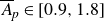 $\overline{A}_{\!p}\in [0.9,1.8]$
) and
$\overline{A}_{\!p}\in [0.9,1.8]$
) and ${\textit{Re}}\lt 0.1$
, our results should therefore be interpreted as qualitative guidance rather than a universal law.
${\textit{Re}}\lt 0.1$
, our results should therefore be interpreted as qualitative guidance rather than a universal law.
In addition, the present framework does not include near-wall effects, particle–particle interactions, non-Newtonian rheology, or unsteady coupling between translation and rotation. Finally, when the closure is used to predict ensemble drag statistics in settling or transport problems, the orientation distribution must be supplied by experiment, DNS or an auxiliary dynamical model; the projected-area law maps orientation statistics into drag statistics, but does not by itself predict the orientation dynamics.
Sensitivity study of (a) mesh size, (b) lateral domain size, (c) orientation number, and (d) particle Reynolds number, for (a,b) the roughest case, (c) the rough grain with $D_{\!f}=2.5$
and
$D_{\!f}=2.5$
and $R_{r}=0.2$
, and (d) the spherical, ellipsoidal (
$R_{r}=0.2$
, and (d) the spherical, ellipsoidal ( $\mathcal{A}_{\mathscr{r}}=0.6023$
) and roughest (
$\mathcal{A}_{\mathscr{r}}=0.6023$
) and roughest ( $D_{\!f}=2.5$
and
$D_{\!f}=2.5$
and $R_{r}=0.35$
) grains at one specific rotation angle.
$R_{r}=0.35$
) grains at one specific rotation angle.

6.4. Physical implications: settling experiments and micromechanics
Revisiting settling-grain-experiment-based empirical equations to predict $C_{\overline{D}}$
of irregular grains at creeping flows (Michaelides & Feng Reference Michaelides and Feng2023), nearly all of them have the same general formulation:
$C_{\overline{D}}$
of irregular grains at creeping flows (Michaelides & Feng Reference Michaelides and Feng2023), nearly all of them have the same general formulation: $C_{\overline{D}}=C_{\overline{D}0}(1+\mathcal{F})$
, with
$C_{\overline{D}}=C_{\overline{D}0}(1+\mathcal{F})$
, with $\mathcal{F}\gt 0$
being a function of shape indices. The drag enhancement in experiments is contradictory to the prevalent view – surface roughness equals drag reduction – in both rough channel flow (Choi et al. Reference Chéron, Evrard and van Wachem2008) and simulations of single rough grains with various rotations. Focusing on the single-grain drag, the analytical derivations of Leith (Reference Leith1987) are also contrary to the general view,
$\mathcal{F}\gt 0$
being a function of shape indices. The drag enhancement in experiments is contradictory to the prevalent view – surface roughness equals drag reduction – in both rough channel flow (Choi et al. Reference Chéron, Evrard and van Wachem2008) and simulations of single rough grains with various rotations. Focusing on the single-grain drag, the analytical derivations of Leith (Reference Leith1987) are also contrary to the general view, $C_{\overline{D}}=C_{\overline{D}0}(1+\mathcal{F})$
. As demonstrated in figure 4(a), higher roughness could induce a net decrease of
$C_{\overline{D}}=C_{\overline{D}0}(1+\mathcal{F})$
. As demonstrated in figure 4(a), higher roughness could induce a net decrease of $C_{\!D}$
, although Leith’s model systematically departs from DNS for non-spherical shapes. Appendix E benchmarks this 0.8 power law against widely used correlations for axisymmetric and irregular shapes; within the Stokes limit, it performs competitively for spheroids (one-angle dependence) and, crucially, generalises to two-angle-dependent bodies (triaxial ellipsoids and rough grains), where many one-angle closures deteriorate.
$C_{\!D}$
, although Leith’s model systematically departs from DNS for non-spherical shapes. Appendix E benchmarks this 0.8 power law against widely used correlations for axisymmetric and irregular shapes; within the Stokes limit, it performs competitively for spheroids (one-angle dependence) and, crucially, generalises to two-angle-dependent bodies (triaxial ellipsoids and rough grains), where many one-angle closures deteriorate.
To explain this paradox, we start with examining the settling grain in a static fluid, concentrating on two parameters: the projected area $A_{\!p}$
, and the steady settling down velocity
$A_{\!p}$
, and the steady settling down velocity $w_{\!f}$
. The experimental drag coefficient is determined by
$w_{\!f}$
. The experimental drag coefficient is determined by $C_{\!D}=2(\rho _{s}-\rho _{\!f})gV_{\!p}/(\rho _{\!f}A_{\!p}w_{\!f}^{2})$
, where
$C_{\!D}=2(\rho _{s}-\rho _{\!f})gV_{\!p}/(\rho _{\!f}A_{\!p}w_{\!f}^{2})$
, where $\rho _{s}$
is the density of the grain. First, although rotated less or more periodically, the gravity-driven grain tends to fall with its maximum
$\rho _{s}$
is the density of the grain. First, although rotated less or more periodically, the gravity-driven grain tends to fall with its maximum $A_{\!p}$
of higher likelihood to be perpendicular to the relative movement direction (Dietrich Reference Dietrich1982). This manifestation could induce lower
$A_{\!p}$
of higher likelihood to be perpendicular to the relative movement direction (Dietrich Reference Dietrich1982). This manifestation could induce lower $w_{\!f}$
of the grain. Note that although in such a type of experiment
$w_{\!f}$
of the grain. Note that although in such a type of experiment $w_{\!f}$
is quantified by the vertically falling down velocity,
$w_{\!f}$
is quantified by the vertically falling down velocity, $w_{f,z}\approx w_{\!f}$
, in fact the grain could dive spirally, and
$w_{f,z}\approx w_{\!f}$
, in fact the grain could dive spirally, and $w_{\!f}=\sqrt{w_{f,x}^{2}+w_{f,y}^{2}+w_{f,z}^{2}}\gt w_{f,z}$
. As demonstrated in a recent study on an experiment on the settling motion of coral grains (Chen et al. Reference Chen2024), the spiral trajectory becomes more tumbling and even chaotic from an elliptical shape in the
$w_{\!f}=\sqrt{w_{f,x}^{2}+w_{f,y}^{2}+w_{f,z}^{2}}\gt w_{f,z}$
. As demonstrated in a recent study on an experiment on the settling motion of coral grains (Chen et al. Reference Chen2024), the spiral trajectory becomes more tumbling and even chaotic from an elliptical shape in the $x$
–
$x$
– $y$
plane with increasing grain irregularity. Further, in their experiments the lateral velocity
$y$
plane with increasing grain irregularity. Further, in their experiments the lateral velocity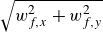 $\sqrt{w_{f,x}^{2}+w_{f,y}^{2}}$
could be enlarged without an asymptotic value. This indicates that using the approximation
$\sqrt{w_{f,x}^{2}+w_{f,y}^{2}}$
could be enlarged without an asymptotic value. This indicates that using the approximation $w_{\!f}\approx w_{f,z}$
could highly underestimate the falling down velocity for grains with higher roughness. Second, quantifying the inconsistent values of
$w_{\!f}\approx w_{f,z}$
could highly underestimate the falling down velocity for grains with higher roughness. Second, quantifying the inconsistent values of $A_{\!p}$
is non-trivial during the falling down process of the grain with quasi-periodic rotations. Considering the ease of measuring grain volume by
$A_{\!p}$
is non-trivial during the falling down process of the grain with quasi-periodic rotations. Considering the ease of measuring grain volume by $V_{\!p}={m_{s}}/{\rho _{s}}$
with the grain mass
$V_{\!p}={m_{s}}/{\rho _{s}}$
with the grain mass $m_{s}$
, the projected area
$m_{s}$
, the projected area $A_{\textit{eq}}$
of volume-equivalent sphere is always implemented instead. Such a value can be lower by up to 80 % of the maximum
$A_{\textit{eq}}$
of volume-equivalent sphere is always implemented instead. Such a value can be lower by up to 80 % of the maximum $A_{\!p}$
, as illustrated in figure 6. The significant underestimations of both
$A_{\!p}$
, as illustrated in figure 6. The significant underestimations of both $w_{\!f}$
and
$w_{\!f}$
and $A_{\!p}$
are attributed to the overestimation of
$A_{\!p}$
are attributed to the overestimation of $C_{\!D}$
in this series of experiments. The present framework yields testable predictions for such experiments: (i) if the orientation distribution during fall is skewed towards large
$C_{\!D}$
in this series of experiments. The present framework yields testable predictions for such experiments: (i) if the orientation distribution during fall is skewed towards large $\overline{A}_{\!p}$
, then the measured
$\overline{A}_{\!p}$
, then the measured $C_{\overline{D}}$
distribution should match the Fréchet-type upper tail implied by (4.2); and (ii) measuring the distribution of
$C_{\overline{D}}$
distribution should match the Fréchet-type upper tail implied by (4.2); and (ii) measuring the distribution of $\overline{A}_{\!p}$
(e.g. via imaging or equivalent-ellipsoid approximation) suffices to generate an a priori prediction of the full
$\overline{A}_{\!p}$
(e.g. via imaging or equivalent-ellipsoid approximation) suffices to generate an a priori prediction of the full $C_{\overline{D}}$
distribution for a given morphology via the 0.8 power mapping.
$C_{\overline{D}}$
distribution for a given morphology via the 0.8 power mapping.
Intuitively, one may ask why the general formula $C_{\overline{D}}=C_{\overline{D}0}(1+\mathcal{F})$
and its inference – roughness means drag enhancement – are so popular. Although the mean value is negatively related to
$C_{\overline{D}}=C_{\overline{D}0}(1+\mathcal{F})$
and its inference – roughness means drag enhancement – are so popular. Although the mean value is negatively related to $R_{r}$
, the standard deviation even vanishes at extremely low
$R_{r}$
, the standard deviation even vanishes at extremely low $R_{r}$
in our DNS with fixed grain rotation; this facilitates the possibility where
$R_{r}$
in our DNS with fixed grain rotation; this facilitates the possibility where $C_{\overline{D}}$
of high
$C_{\overline{D}}$
of high $R_{r}$
could be larger than that of low
$R_{r}$
could be larger than that of low $R_{r}$
, resulting in roughness-induced drag enhancement in experiments. One may argue that in the situation of complete drag reduction, i.e. for extremely high
$R_{r}$
, resulting in roughness-induced drag enhancement in experiments. One may argue that in the situation of complete drag reduction, i.e. for extremely high $R_{r}$
and
$R_{r}$
and $D_{\!f}$
,
$D_{\!f}$
, $C_{\overline{D}}$
is always smaller than
$C_{\overline{D}}$
is always smaller than $C_{\overline{D}0}$
, and no drag improvement could be encountered. Considering the narrow ranges of natural grains (
$C_{\overline{D}0}$
, and no drag improvement could be encountered. Considering the narrow ranges of natural grains ( $R_{r}\lt 0.1$
and
$R_{r}\lt 0.1$
and $D_{\!f}\lt 2.3$
), for which settling experiments are conducted and are mostly from the geoscience community for sedimentary study, complete drag reduction is less likely to happen. To bypass the large uncertainty in grain rotation during settling, we propose a power law
$D_{\!f}\lt 2.3$
), for which settling experiments are conducted and are mostly from the geoscience community for sedimentary study, complete drag reduction is less likely to happen. To bypass the large uncertainty in grain rotation during settling, we propose a power law $C_{\overline{D}}=a\overline{A}_{\!p}^{-0.8}$
to introduce the rotational dependence of drag coefficient for the single aspherical grain of various rotation angles.
$C_{\overline{D}}=a\overline{A}_{\!p}^{-0.8}$
to introduce the rotational dependence of drag coefficient for the single aspherical grain of various rotation angles.
At the grain scale, the DNS results indicate that roughness-induced drag reduction originates mainly from the friction-drag contribution. Local ridges intensify shear only over limited surface patches, whereas dimples and concave regions broaden low-shear zones over a larger fraction of the surface; the net effect is therefore a downward shift of the friction-drag contribution, while the pressure-drag contribution remains comparatively insensitive to morphology. This interpretation also explains why the prefactor $a$
decreases as grains depart from the purely convex limit. Increasing concavity weakens the effective skin-friction contribution without requiring a comparable reduction in pressure drag.
$a$
decreases as grains depart from the purely convex limit. Increasing concavity weakens the effective skin-friction contribution without requiring a comparable reduction in pressure drag.
7. Conclusions
In conclusion, this study comprehensively investigates the impact of grain morphology and rotation on drag at creeping flows. Using spherical harmonics, a series of rough grains, with irregularities quantified by relative roughness $R_{r}$
and fractal dimension
$R_{r}$
and fractal dimension $D_{\!f}$
, are simulated. As the grain surface becomes more angular with increasing
$D_{\!f}$
, are simulated. As the grain surface becomes more angular with increasing $R_{r}$
and
$R_{r}$
and $D_{\!f}$
, a stronger drag reduction is observed, demonstrating much smaller
$D_{\!f}$
, a stronger drag reduction is observed, demonstrating much smaller $C_{\overline{D}}$
than that of a smooth sphere. Aided by rotation dependence, the drag paradox between settling experiments and the prevalent view in rough channel flow is successfully explained. The microanalysis underscores that the primary cause of drag reduction is decreased skin friction due to flow dynamics around ridges and dimples. This mechanistic picture – ridge-enhanced shear but dimple-broadened low-shear regions – explains why the pressure-drag contribution averages nearly unchanged across morphologies, whereas the friction-drag contribution shifts downwards, demonstrated by figures 7 and 8. Importantly, the drag coefficient distribution for a given rough grain universally adheres to the Weibullian pattern. Beyond shape class, we further observe that the prefactor
$C_{\overline{D}}$
than that of a smooth sphere. Aided by rotation dependence, the drag paradox between settling experiments and the prevalent view in rough channel flow is successfully explained. The microanalysis underscores that the primary cause of drag reduction is decreased skin friction due to flow dynamics around ridges and dimples. This mechanistic picture – ridge-enhanced shear but dimple-broadened low-shear regions – explains why the pressure-drag contribution averages nearly unchanged across morphologies, whereas the friction-drag contribution shifts downwards, demonstrated by figures 7 and 8. Importantly, the drag coefficient distribution for a given rough grain universally adheres to the Weibullian pattern. Beyond shape class, we further observe that the prefactor $a$
of the power law
$a$
of the power law $C_{\overline{D}}=a\overline{A}_{\!p}^{-0.8}$
, analytically derived from ellipsoidal grains, correlates with global convexity
$C_{\overline{D}}=a\overline{A}_{\!p}^{-0.8}$
, analytically derived from ellipsoidal grains, correlates with global convexity $\mathcal{C}_{\mathcal{X}} : a\rightarrow 24$
as
$\mathcal{C}_{\mathcal{X}} : a\rightarrow 24$
as $\mathcal{C}_{\mathcal{X}}\rightarrow 1$
(purely convex limit, such as PCA-equivalent ellipsoids), and
$\mathcal{C}_{\mathcal{X}}\rightarrow 1$
(purely convex limit, such as PCA-equivalent ellipsoids), and $a\leq 24$
for
$a\leq 24$
for $\mathcal{C}_{\mathcal{X}}\lt 1$
; this provides a compact way to port morphology into continuum closures (see Appendix A for
$\mathcal{C}_{\mathcal{X}}\lt 1$
; this provides a compact way to port morphology into continuum closures (see Appendix A for $\mathcal{C}_{\mathcal{X}}$
, and Appendix D for
$\mathcal{C}_{\mathcal{X}}$
, and Appendix D for $a$
).
$a$
).
Complementary lift force results (Appendix F) indicate that increasing global irregularity, i.e. lower aspect ratio or sphericity, by higher $R_{r}$
elevates the mean lift and its scatter, whereas increased local roughness by higher
$R_{r}$
elevates the mean lift and its scatter, whereas increased local roughness by higher $D_{\!f}$
tends to narrow their distributions, consistent with our micromechanics. These trends are relevant whenever lateral migration or preferential alignment matters, but lift is not needed to deploy the proposed drag closure.
$D_{\!f}$
tends to narrow their distributions, consistent with our micromechanics. These trends are relevant whenever lateral migration or preferential alignment matters, but lift is not needed to deploy the proposed drag closure.
Finally, through a comprehensive comparison with existing models, we show that among existing correlations, the present law provides a unifying, geometry-driven predictor across one- and two-angle-dependent shapes in the creeping-flow limit, offering a compact bridge from micro-scale morphology to macro-scale drag for irregular grains. The present closure is derived and validated strictly in the Stokes regime for isolated grains in unbounded Newtonian fluids. It does not account for near-wall effects, particle–particle interactions, or finite- ${\textit{Re}}$
inertia. For quantitative use beyond the Stokes regime, we recommend combining the
${\textit{Re}}$
inertia. For quantitative use beyond the Stokes regime, we recommend combining the ${\overline{A}}_{\!p}^{-0.8}$
dependence with an inertial correction to
${\overline{A}}_{\!p}^{-0.8}$
dependence with an inertial correction to $a$
calibrated at small
$a$
calibrated at small ${\textit{Re}}$
(see Appendix B), and where needed, an orientation model informed by measured
${\textit{Re}}$
(see Appendix B), and where needed, an orientation model informed by measured $P_{s}(\overline{A}_{\!p})$
.
$P_{s}(\overline{A}_{\!p})$
.
Funding
This work is supported by the National Science and Technology Major Project for Deep Earth Probe and Mineral Resources Exploration (no. 2025ZD1008302), the National Natural Science Foundation of China (grant no. 12202342, and the Excellent Young Scientists Fund (overseas) for D.W.), and the Australian Research Council (Discovery Early Career Award, grant no. DE240101106).
Declaration of interests
The authors report no conflict of interest.
Appendix A. Equivalent ellipsoids and shape indices of rough grains
We determine the axes-equivalent ellipsoids for the rough particles shown in figure 1(a) by three-dimensional shape analysis based on PCA of spatial coordinates of all surficial particle points. The relevant shape parameters, including aspect ratio, elongation, flatness, roundness, sphericity and convexity, are calculated accordingly; see tables 1, 2, 3, 4, 5 and 6. The quantification method can be found in Zhao & Wang (Reference Zhao and Wang2016).
Aspect ratio ( $\mathcal{A}_{\mathscr{r}}$
).
$\mathcal{A}_{\mathscr{r}}$
).

Elongation ( $\mathcal{E}_{\mathscr{i}}$
).
$\mathcal{E}_{\mathscr{i}}$
).

Flatness ( $\mathcal{F}_{\mathscr{i}}$
).
$\mathcal{F}_{\mathscr{i}}$
).

Roundness ( $\mathcal{R}$
).
$\mathcal{R}$
).

Sphericity ( $\mathcal{S}$
).
$\mathcal{S}$
).

Convexity ( $\mathcal{C}_{\mathcal{X}}$
).
$\mathcal{C}_{\mathcal{X}}$
).

The ratio of the minimum to maximum radial length ( $\mathcal{A}_{\mathcal{R}}$
).
$\mathcal{A}_{\mathcal{R}}$
).

Shape parameters for ellipsoidal, oblate and prolate grains.

Note: the first four rows are ellipsoidal grains, while the 5th–10th rows are oblate grains, and the rest are prolate grains.
Appendix B. Sensitivity study of mesh size, lateral domain size, orientation number and Reynolds number
We perform a mesh dependence study for the roughest grain ( $D_{\!f}=2.5$
and
$D_{\!f}=2.5$
and $R_{r}=0.35$
). The case with
$R_{r}=0.35$
). The case with $h=3.7\times 10^{-4}d_{\textit{eq}}$
is taken as a ground truth. As shown in figure 9(a), numerical convergence is guaranteed for
$h=3.7\times 10^{-4}d_{\textit{eq}}$
is taken as a ground truth. As shown in figure 9(a), numerical convergence is guaranteed for $h=1.2\times 10^{-2}d_{\textit{eq}}$
, with relative error less than 6 %. Besides, using the roughest grain, we also test the fluid domain size effects. As shown in figure 9(b), in which the result with the largest domain
$h=1.2\times 10^{-2}d_{\textit{eq}}$
, with relative error less than 6 %. Besides, using the roughest grain, we also test the fluid domain size effects. As shown in figure 9(b), in which the result with the largest domain $L_{y}=L_{z}=24d_{\textit{eq}}$
is taken as a ground truth, the selected domain size
$L_{y}=L_{z}=24d_{\textit{eq}}$
is taken as a ground truth, the selected domain size $L_{y}=L_{z}=20d_{\textit{eq}}$
can guarantee a negligible boundary effect.
$L_{y}=L_{z}=20d_{\textit{eq}}$
can guarantee a negligible boundary effect.
We then perform a sensitivity study of orientation number, and two orientation numbers $N=51$
and
$N=51$
and $N=87$
are investigated. Their statistical results are compared in figure 9(c), and the fitting parameters are presented in table 9. We also perform a sensitivity study of Reynolds number on the sphere, the ellipsoid (
$N=87$
are investigated. Their statistical results are compared in figure 9(c), and the fitting parameters are presented in table 9. We also perform a sensitivity study of Reynolds number on the sphere, the ellipsoid ( $\mathcal{A}_{\mathscr{r}}=0.6023$
) and the roughest grain (
$\mathcal{A}_{\mathscr{r}}=0.6023$
) and the roughest grain ( $D_{\!f}=2.5$
and
$D_{\!f}=2.5$
and $R_{r}=0.35$
). As shown in figure 9(d), these three geometries fall within the same Stokes range, i.e.
$R_{r}=0.35$
). As shown in figure 9(d), these three geometries fall within the same Stokes range, i.e. ${\textit{Re}}\lt 0.1$
.
${\textit{Re}}\lt 0.1$
.
Fitting parameters.

Appendix C. Theoretical derivations of
$\boldsymbol{{C}_{\!{D}}}$
versus
$\boldsymbol{{A}_{\!{p}}}$
for triaxial-ellipsoidal grains


An ellipsoidal surface can be represented in the Cartesian coordinate system as
 \begin{equation}\frac{x^{2}}{\mathscr{a}^{2}}+\frac{y^{2}}{\mathscr{a}^{2}\left(1-\epsilon \right)^{2}}+\frac{z^{2}}{\mathscr{a}^{2}\left(1-\epsilon \right)^{2}\left(1-\varepsilon \right)^{2}}=1,\end{equation}
where $0\lt \epsilon \ll 1$
and
$0\lt \epsilon \ll 1$
and $0\lt \varepsilon \ll 1$
. According to Vickers (Reference Wadell1996), the projected area in the direction of
$0\lt \varepsilon \ll 1$
. According to Vickers (Reference Wadell1996), the projected area in the direction of $\boldsymbol{n}=(\ell,\mathscr{m},\mathscr{n} )=(\sin \Theta \cos \Phi , \sin \Theta \sin \Phi , \cos \Theta)$
of an ellipsoid,
$\boldsymbol{n}=(\ell,\mathscr{m},\mathscr{n} )=(\sin \Theta \cos \Phi , \sin \Theta \sin \Phi , \cos \Theta)$
of an ellipsoid, $({x^{2}}/{\mathscr{u}^{2}})+({y^{2}}/{\mathscr{v}^{2}})+({z^{2}}/{\mathscr{w}^{2}})=1$
, is
$({x^{2}}/{\mathscr{u}^{2}})+({y^{2}}/{\mathscr{v}^{2}})+({z^{2}}/{\mathscr{w}^{2}})=1$
, is $A_{\!p}=\pi \sqrt{\ell^{2}\mathscr{v}^{2}\mathscr{w}^{2}+\mathscr{m}^{2}\mathscr{u}^{2}\mathscr{w}^{2}+\mathscr{n}^{2}\mathscr{u}^{2}\mathscr{v}^{2}}$
. Thus the projected area for a triaxial ellipsoid described in (C1) is
$A_{\!p}=\pi \sqrt{\ell^{2}\mathscr{v}^{2}\mathscr{w}^{2}+\mathscr{m}^{2}\mathscr{u}^{2}\mathscr{w}^{2}+\mathscr{n}^{2}\mathscr{u}^{2}\mathscr{v}^{2}}$
. Thus the projected area for a triaxial ellipsoid described in (C1) is
 \begin{equation}A_{\!p}=\pi \mathscr{a}^{2}\left(1-\epsilon \right)^{2}\left(1-\varepsilon \right)\underset{\mathcal{S}}{\underbrace{\sqrt{\ell^{2}+\mathscr{m}^{2}\left(1-\epsilon \right)^{-2}+\mathscr{n}^{2}\left(1-\varepsilon \right)^{-2}\left(1-\epsilon \right)^{-2}}}}.\end{equation}
Since $A_{\textit{eq}}=\pi {R_{\textit{eq}}}^{2}$
and
$A_{\textit{eq}}=\pi {R_{\textit{eq}}}^{2}$
and $R_{\textit{eq}}=\mathscr{a}(1-\epsilon )^{{2}/{3}}(1-\varepsilon )^{{1}/{3}}$
, by the first-order Taylor approximation of
$R_{\textit{eq}}=\mathscr{a}(1-\epsilon )^{{2}/{3}}(1-\varepsilon )^{{1}/{3}}$
, by the first-order Taylor approximation of $A_{\!p}$
, the normalised projected area towards
$A_{\!p}$
, the normalised projected area towards $\boldsymbol{n}$
can be expressed as
$\boldsymbol{n}$
can be expressed as
 \begin{equation}\overline{A}_{\!p}:= \frac{A_{\!p}}{A_{\textit{eq}}}=\left(1-\epsilon \right)^{\frac{2}{3}}\left(1-\varepsilon \right)^{\frac{1}{3}}\mathcal{S}=1+\epsilon \left(\frac{1}{3}-\ell^{2}\right)+\varepsilon \left(\mathscr{n}^{2}-\frac{1}{3}\right)+\mathcal{O}\left(\epsilon ^{2},\varepsilon ^{2}\right).\end{equation}
According to Oberbeck (Reference Oberbeck1876), at creeping flow, the directional drag force along $\boldsymbol{n}$
on an ellipsoidal grain is
$\boldsymbol{n}$
on an ellipsoidal grain is
 \begin{equation}F_{\!D}\left(\Theta ,\Phi \right)=6\pi \mu _{\!f}R_{\textit{eq}}\,k_{\textit{eff}}\left(\Theta ,\Phi \right)\left| \boldsymbol{u}_{\infty }\right|,\end{equation}
with the effective correction factor $k_{\textit{eff}}(\Theta ,\Phi )$
, when compared with the volume-equivalent sphere, from the drag force tensor,
$k_{\textit{eff}}(\Theta ,\Phi )$
, when compared with the volume-equivalent sphere, from the drag force tensor, $\boldsymbol{K}=\text{diag}(k_{\mathscr{u}},k_{\mathscr{v}},k_{\mathscr{w}})$
:
$\boldsymbol{K}=\text{diag}(k_{\mathscr{u}},k_{\mathscr{v}},k_{\mathscr{w}})$
:
 \begin{equation}k_{\textit{eff}}\left(\Theta ,\Phi \right)=k_{\mathscr{u}}\ell^{2}+k_{\mathscr{v}}\mathscr{m}^{2}+k_{\mathscr{w}}\mathscr{n}^{2}.\end{equation}
The components of $\boldsymbol{K}$
can be denoted as
$\boldsymbol{K}$
can be denoted as
 \begin{equation}k_{i}=\frac{8}{3}\frac{\left(\mathscr{a}^{3}\left(1-\epsilon \right)^{2}\left(1-\varepsilon \right)\right)^{2/3}}{\chi _{0}+{a_{i}}^{2}\alpha _{i}},\quad i=\mathscr{u},\mathscr{v},\mathscr{w},\end{equation}
with $a_{\mathscr{u}}=\mathscr{a}$
,
$a_{\mathscr{u}}=\mathscr{a}$
, $a_{\mathscr{v}}=\mathscr{a}(1-\epsilon )$
and
$a_{\mathscr{v}}=\mathscr{a}(1-\epsilon )$
and $a_{\mathscr{w}}=\mathscr{a}(1-\epsilon )(1-\varepsilon )$
. Here,
$a_{\mathscr{w}}=\mathscr{a}(1-\epsilon )(1-\varepsilon )$
. Here, $\chi _{0}$
and
$\chi _{0}$
and $\alpha _{i}$
are respectively described using Carlson symmetric elliptic integrals of the first and second kinds,
$\alpha _{i}$
are respectively described using Carlson symmetric elliptic integrals of the first and second kinds, $R_{\!F}(x,y,z)={1}/{2}{\int }_{0}^{\infty }{{\rm d}t}/{\sqrt{(x+t)(y+t)(z+t)}}$
and
$R_{\!F}(x,y,z)={1}/{2}{\int }_{0}^{\infty }{{\rm d}t}/{\sqrt{(x+t)(y+t)(z+t)}}$
and $R_{\!D}(x,y,z)={3}/{2}{\int }_{0}^{\infty }{{\rm d}t}/((z+t)\sqrt{(x+t)(y+t)(z+t)})$
:
$R_{\!D}(x,y,z)={3}/{2}{\int }_{0}^{\infty }{{\rm d}t}/((z+t)\sqrt{(x+t)(y+t)(z+t)})$
:
 \begin{align}\chi _{0}&=2\big(\mathscr{a}^{3}\left(1-\epsilon \right)^{2}\left(1-\varepsilon \right)\big) R_{\!F}\big(\mathscr{a}^{2},\mathscr{a}^{2}\left(1-\epsilon \right)^{2},\mathscr{a}^{2}\left(1-\epsilon \right)^{2}\left(1-\varepsilon \right)^{2}\big), \\[-12pt]\nonumber\end{align}
 \begin{align}\alpha _{i}&=\begin{cases} \alpha _{\mathscr{u}}=\dfrac{2\left(\mathscr{a}^{3}\left(1-\epsilon \right)^{2}\left(1-\varepsilon \right)\right)}{\mathscr{a}^{2}}R_{\!D}\left(\mathscr{a}^{2}\left(1-\epsilon \right)^{2},\mathscr{a}^{2}\left(1-\epsilon \right)^{2}\left(1-\varepsilon \right)^{2},\mathscr{a}^{2}\right)\!,\\[10pt] \alpha _{\mathscr{v}}=\dfrac{2\left(\mathscr{a}^{3}\left(1-\epsilon \right)^{2}\left(1-\varepsilon \right)\right)}{\mathscr{a}^{2}\left(1-\epsilon \right)^{2}}R_{\!D}\left(\mathscr{a}^{2}\left(1-\epsilon \right)^{2}\left(1-\varepsilon \right)^{2},\mathscr{a}^{2},\mathscr{a}^{2}\left(1-\epsilon \right)^{2}\right)\!,\\[12pt] \alpha _{\mathscr{w}}=\dfrac{2\left(\mathscr{a}^{3}\left(1-\epsilon \right)^{2}\left(1-\varepsilon \right)\right)}{\mathscr{a}^{2}\left(1-\epsilon \right)^{2}\left(1-\varepsilon \right)^{2}}R_{\!D}\left(\mathscr{a}^{2},\mathscr{a}^{2}\left(1-\epsilon \right)^{2},\mathscr{a}^{2}\left(1-\epsilon \right)^{2}\left(1-\varepsilon \right)^{2}\right)\!. \end{cases} \end{align}
According to the homogeneity of the first kind Carlson symmetric elliptic integral $R_{\!F}(\lambda x,\lambda y,\lambda z)=\lambda ^{-{1}/{2}}\,R_{\!F}(x,y,z)$
,
$R_{\!F}(\lambda x,\lambda y,\lambda z)=\lambda ^{-{1}/{2}}\,R_{\!F}(x,y,z)$
,
 \begin{equation}\chi _{0}=2\mathscr{a}^{2}\left(1-2\epsilon -\varepsilon \right) R_{\!F}\left(1,1-2\epsilon ,1-2\epsilon -2\varepsilon \right).\end{equation}
Via the Laurent series expansion $R_{\!F}(1,1-2\epsilon ,1-2\epsilon -2\varepsilon )=1-(0+(-2\epsilon )+{}(-2\epsilon -2\varepsilon ))/{10}+\mathcal{O}(\epsilon ^{2},\varepsilon ^{2})$
, we get
$R_{\!F}(1,1-2\epsilon ,1-2\epsilon -2\varepsilon )=1-(0+(-2\epsilon )+{}(-2\epsilon -2\varepsilon ))/{10}+\mathcal{O}(\epsilon ^{2},\varepsilon ^{2})$
, we get
 \begin{equation}\chi _{0}=2\mathscr{a}^{2}\left(1-\frac{8}{5}\epsilon -\frac{4}{5}\varepsilon \right)+\mathcal{O}\big(\epsilon ^{2},\varepsilon ^{2}\big).\end{equation}
Again, according to the homogeneity of the second kind Carlson symmetric elliptic integral $R_{\!D}(\lambda x,\lambda y,\lambda z)=\lambda ^{-{3}/{2}}\,R_{\!D}(x,y,z)$
and the Laurent series expansion around
$R_{\!D}(\lambda x,\lambda y,\lambda z)=\lambda ^{-{3}/{2}}\,R_{\!D}(x,y,z)$
and the Laurent series expansion around $R_{\!D}(1,1,1)$
with
$R_{\!D}(1,1,1)$
with $\varDelta _{1}$
and
$\varDelta _{1}$
and $\varDelta _{2}$
both infinitesimal,
$\varDelta _{2}$
both infinitesimal, $R_{\!D}(1+\varDelta _{1},1+\varDelta _{2},1)=1-({3}/{10})(\varDelta _{1}+\varDelta _{2})+\mathcal{O}(\varDelta_{1}^{2},\varDelta_{2}^{2})$
,
$R_{\!D}(1+\varDelta _{1},1+\varDelta _{2},1)=1-({3}/{10})(\varDelta _{1}+\varDelta _{2})+\mathcal{O}(\varDelta_{1}^{2},\varDelta_{2}^{2})$
,
 \begin{equation}\alpha _{i}=\begin{cases} \alpha _{\mathscr{u}}=\dfrac{2}{3}\mathscr{a}\left(1-\dfrac{4}{5}\epsilon -\dfrac{2}{5}\varepsilon \right)+\mathcal{O}\left(\epsilon ^{2},\varepsilon ^{2}\right)\!,\\[10pt] \alpha _{\mathscr{v}}=\dfrac{2}{3}\mathscr{a}\left(1+\dfrac{7}{5}\epsilon -\dfrac{2}{5}\varepsilon \right)+\mathcal{O}\left(\epsilon ^{2},\varepsilon ^{2}\right)\!,\\[10pt] \alpha _{\mathscr{w}}=\dfrac{2}{3}\mathscr{a}\left(1+\dfrac{7}{5}\epsilon +\dfrac{9}{5}\varepsilon \right)+\mathcal{O}\left(\epsilon ^{2},\varepsilon ^{2}\right). \end{cases}\end{equation}
Submit (C10) and (C11) to (C6):
 \begin{equation}k_{i}=\begin{cases} k_{\mathscr{u}}=1-\dfrac{2}{15}\epsilon -\dfrac{1}{15}\varepsilon +\mathcal{O}\left(\epsilon ^{2},\varepsilon ^{2}\right)\!,\\[10pt] k_{\mathscr{v}}=1+\dfrac{1}{15}\epsilon -\dfrac{1}{15}\varepsilon +\mathcal{O}\left(\epsilon ^{2},\varepsilon ^{2}\right)\!,\\[10pt] k_{\mathscr{w}}=1+\dfrac{1}{15}\epsilon +\dfrac{2}{15}\varepsilon +\mathcal{O}\left(\epsilon ^{2},\varepsilon ^{2}\right). \end{cases}\end{equation}
Import it into (C5):
 \begin{equation}k_{\textit{eff}}\left(\Theta ,\Phi \right)=1+\frac{1-3\ell^{2}}{15}\epsilon +\frac{3\mathscr{n}^{2}-1}{15}\varepsilon +\mathcal{O}\big(\epsilon ^{2},\varepsilon ^{2}\big).\end{equation}
Interestingly, it is found that the angle-dependent term $({1}/{3}-\ell^{2})\epsilon +(\mathscr{n}^{2}-{1}/{3})\varepsilon$
of
$({1}/{3}-\ell^{2})\epsilon +(\mathscr{n}^{2}-{1}/{3})\varepsilon$
of $\overline{A}_{\!p}$
in (C3) appears in the equation to denote
$\overline{A}_{\!p}$
in (C3) appears in the equation to denote $k_{\textit{eff}}(\Theta ,\Phi )$
. Then go back to the
$k_{\textit{eff}}(\Theta ,\Phi )$
. Then go back to the $({1}/{\textit{Re}})$
-normalised drag coefficient
$({1}/{\textit{Re}})$
-normalised drag coefficient
 \begin{equation}C_{\overline{D}}\left(\Theta ,\Phi \right):={\textit{Re}}\,C_{\!D}\left(\Theta ,\Phi \right)={\textit{Re}}\,\frac{F_{\!D}\left(\Theta ,\Phi \right)}{\dfrac{1}{2}\rho _{\!f}\left| \boldsymbol{u}_{\infty }\right| ^{2}A_{\!p}}=24\,\frac{k_{\textit{eff}}\left(\Theta ,\Phi \right)}{\overline{A}_{\!p}}.\end{equation}
Since $\overline{A}_{\!p}\approx 1+\epsilon ({1}/{3}-\ell^{2})+\varepsilon (\mathscr{n}^{2}-{1}/{3})$
and
$\overline{A}_{\!p}\approx 1+\epsilon ({1}/{3}-\ell^{2})+\varepsilon (\mathscr{n}^{2}-{1}/{3})$
and $| \epsilon ({1}/{3}-\ell^{2})+\varepsilon (\mathscr{n}^{2}-{1}/{3})| \ll 1$
,
$| \epsilon ({1}/{3}-\ell^{2})+\varepsilon (\mathscr{n}^{2}-{1}/{3})| \ll 1$
, $[1+\epsilon ({1}/{3}-\ell^{2})+\varepsilon (\mathscr{n}^{2}-{1}/{3})]^{-1}\approx 1-\epsilon ({1}/{3}-\ell^{2})-\varepsilon (\mathscr{n}^{2}-{1}/{3})\rightarrow {1}/{\overline{A}_{\!p}}\approx 1-\epsilon ({1}/{3}-\ell^{2})-\varepsilon (\mathscr{n}^{2}-{1}/{3})$
. Then submitting it and (C13)–(C14), we arrive at
$[1+\epsilon ({1}/{3}-\ell^{2})+\varepsilon (\mathscr{n}^{2}-{1}/{3})]^{-1}\approx 1-\epsilon ({1}/{3}-\ell^{2})-\varepsilon (\mathscr{n}^{2}-{1}/{3})\rightarrow {1}/{\overline{A}_{\!p}}\approx 1-\epsilon ({1}/{3}-\ell^{2})-\varepsilon (\mathscr{n}^{2}-{1}/{3})$
. Then submitting it and (C13)–(C14), we arrive at ${C_{\overline{D}}(\Theta ,\Phi )}/{24}=1-({4}/{5})[\epsilon ({1}/{3}-\ell^{2})+\varepsilon (\mathscr{n}^{2}-{1}/{3})]+\mathcal{O}(\epsilon ^{2},\varepsilon ^{2})=1-({4}/{5})(\overline{A}_{\!p}-1)+\mathcal{O}(\epsilon ^{2},\varepsilon ^{2})$
. According to the binomial theorem and
${C_{\overline{D}}(\Theta ,\Phi )}/{24}=1-({4}/{5})[\epsilon ({1}/{3}-\ell^{2})+\varepsilon (\mathscr{n}^{2}-{1}/{3})]+\mathcal{O}(\epsilon ^{2},\varepsilon ^{2})=1-({4}/{5})(\overline{A}_{\!p}-1)+\mathcal{O}(\epsilon ^{2},\varepsilon ^{2})$
. According to the binomial theorem and $| \overline{A}_{\!p}-1| \ll 1$
, we get
$| \overline{A}_{\!p}-1| \ll 1$
, we get
 \begin{equation}\frac{C_{\overline{D}}\left(\Theta ,\Phi \right)}{24}\approx \left[1+\left(\overline{A}_{\!p}-1\right)\right]^{-{4}/{5}}+\mathcal{O}\big(\epsilon ^{2},\varepsilon ^{2}\big)\rightarrow C_{\overline{D}}\left(\Theta ,\Phi \right)\approx 24\overline{A}_{\!p}^{-0.8}.\end{equation}
Appendix D. Power-law parameters
The parameters $a$
involved in the power law
$a$
involved in the power law $C_{\overline{D}}(\overline{A}_{\!p})=a\overline{A}_{\!p}^{-0.8}$
for each rough particle are summarised in table 10. The R-squared values of these fittings are summarised in table 11.
$C_{\overline{D}}(\overline{A}_{\!p})=a\overline{A}_{\!p}^{-0.8}$
for each rough particle are summarised in table 10. The R-squared values of these fittings are summarised in table 11.
Scale coefficient ( $a$
) of all rough grains.
$a$
) of all rough grains.

Goodness-of-fit measures (R-squared values) of all rough grains.

Appendix E. Comparison with existing models
We compared the predictability of existing models – including Ganser (Reference Ganser1993), Tran-Cong, Gay & Michaelides (Reference Tran-Cong, Gay and Michaelides2004), Hölzer & Sommerfeld (Reference Hughes and Mallet2008), Bagheri & Bonadonna (Reference Bagheri and Bonadonna2016), Song et al. (Reference Song, Xu, Li, Pang and Zhu2017), Feng & Michaelides (Reference Feng and Michaelides2023) and Happel & Brenner (Reference Happel and Brenner1983) – with our 0.8 power law. Specific formulas of these models are summarised in table 12. The latter two models are derived from the Stokes equations and only account for one-rotation-angle dependence, while the others are for two-rotation-angle dependence. Figure 10 shows the comparison results for the roughest grain, a spherocylinder – which is often used to represent slender fibres with a significantly large aspect ratio – an oblate and a prolate. As indicated in our theoretical derivation based on Happel & Brenner (Reference Happel and Brenner1983), our 0.8 power law applies in the Stokes regime as confirmed again here, and it is surprisingly found that it can cover a wide range of geometries as per these comparison results. For other models, e.g. Ganser (Reference Ganser1993), Tran-Cong et al. (Reference Tran-Cong, Gay and Michaelides2004), Song et al. (Reference Song, Xu, Li, Pang and Zhu2017) and Feng & Michaelides (Reference Feng and Michaelides2023), they aimed to suit a wide range of ${\textit{Re}}$
, usually from 0.1 to 100. Considering that fitting cannot be avoided for irregular shapes, their emphasis on higher-
${\textit{Re}}$
, usually from 0.1 to 100. Considering that fitting cannot be avoided for irregular shapes, their emphasis on higher- ${\textit{Re}}$
cases compromises performance in the low-
${\textit{Re}}$
cases compromises performance in the low- ${\textit{Re}}$
range.
${\textit{Re}}$
range.
Typically existing predictive models for drag coefficients.

Comparison of models for (a) the roughest grain ( $D_{\!f}=2.5$
and
$D_{\!f}=2.5$
and $R_{r}=0.35$
), (b) a spherocylinder (
$R_{r}=0.35$
), (b) a spherocylinder ( $\mathcal{A}_{\mathscr{r}}=2.5$
), (c) an oblate (
$\mathcal{A}_{\mathscr{r}}=2.5$
), (c) an oblate ( $\mathcal{A}_{\mathscr{r}}=0.7$
) and (d) a prolate (
$\mathcal{A}_{\mathscr{r}}=0.7$
) and (d) a prolate ( $\mathcal{A}_{\mathscr{r}}=1.7$
). All results are presented in the log-log scale.
$\mathcal{A}_{\mathscr{r}}=1.7$
). All results are presented in the log-log scale.

Appendix F. Lift coefficient of aspherical grains
From DNS results, we further calculate the lift coefficient $C_{L}$
, which is defined as
$C_{L}$
, which is defined as
 \begin{equation}C_{L}=\frac{F_{L}}{\left(\dfrac{1}{2}\rho _{\!f}\left| \boldsymbol{u}_{\infty }\right| ^{2}A_{\!p}\right)},\end{equation}
where $F_{L}$
is the magnitude of the grain lift force. Similarly to
$F_{L}$
is the magnitude of the grain lift force. Similarly to $C_{\overline{D}}$
,
$C_{\overline{D}}$
, $C_{L}$
is normalised as
$C_{L}$
is normalised as $C_{\overline{L}}={\textit{Re}}\,C_{L}$
; further, its components can be decomposed to a pressure part
$C_{\overline{L}}={\textit{Re}}\,C_{L}$
; further, its components can be decomposed to a pressure part $C_{\overline{L}}^{p}$
and a friction part
$C_{\overline{L}}^{p}$
and a friction part $C_{\overline{L}}^{f}$
. Notably, in (F1),
$C_{\overline{L}}^{f}$
. Notably, in (F1), $A_{\!p}$
is implemented instead of
$A_{\!p}$
is implemented instead of $A_{\textit{eq}}$
, the projected area of the volume-equivalent sphere. We have confirmed that when
$A_{\textit{eq}}$
, the projected area of the volume-equivalent sphere. We have confirmed that when $A_{\textit{eq}}$
is used to define both
$A_{\textit{eq}}$
is used to define both $C_{\!D}$
and
$C_{\!D}$
and $C_{L}$
, the traditional sine–cosine law
$C_{L}$
, the traditional sine–cosine law
 \begin{equation} C_{\!L}(\Theta )=\underset{\Delta C_{\!D}}{\underbrace{(C_{D,\Theta =\frac{\pi }{2}}-C_{D,\Theta =0})}}\sin \Theta \cos \Theta, \end{equation}
is encountered for lift coefficients of the spheroidal grain simulated by our DNS. In fact, we have considered lift forces by seeking a power law similar to $C_{\overline{D}}\propto \overline{A}_{\!p}^{-0.8}$
, since for irregularly shaped grains, even in the Stokes regime, non-zero lift forces are always encountered on the grain surface. However, it is a non-trivial task to find a roughly monotonic relationship between lift coefficients and
$C_{\overline{D}}\propto \overline{A}_{\!p}^{-0.8}$
, since for irregularly shaped grains, even in the Stokes regime, non-zero lift forces are always encountered on the grain surface. However, it is a non-trivial task to find a roughly monotonic relationship between lift coefficients and $\overline{A}_{\!p}$
for all grain shapes in this study.
$\overline{A}_{\!p}$
for all grain shapes in this study.
As suggested in Jeffery (Reference Jeffery1922), only the first-order terms in the Stokes equations are considered to simplify the analysis on resultant force due to the translational motion between the ellipsoid and the fluid; we analytically show the relationship between $C_{\overline{L}}$
and
$C_{\overline{L}}$
and $\overline{A}_{\!p}$
for two spheroidal grains and one triaxial-ellipsoidal grain, as shown in figure 11. It is obvious that even for the slightly aspherical spheroidal shape, the
$\overline{A}_{\!p}$
for two spheroidal grains and one triaxial-ellipsoidal grain, as shown in figure 11. It is obvious that even for the slightly aspherical spheroidal shape, the $C_{\overline{L}}$
–
$C_{\overline{L}}$
– $\overline{A}_{\!p}$
curve is non-monotonic; except for the highest value, one specific value of
$\overline{A}_{\!p}$
curve is non-monotonic; except for the highest value, one specific value of $C_{\overline{L}}$
corresponds to two
$C_{\overline{L}}$
corresponds to two $\overline{A}_{\!p}$
values, demonstrated in figures 11(a) and 11(b). The situation is more complex for triaxial-ellipsoidal shapes, as in figure 11(c), where one specific value of
$\overline{A}_{\!p}$
values, demonstrated in figures 11(a) and 11(b). The situation is more complex for triaxial-ellipsoidal shapes, as in figure 11(c), where one specific value of $C_{\overline{L}}$
might correspond to one, three or an unlimited number of
$C_{\overline{L}}$
might correspond to one, three or an unlimited number of $\overline{A}_{\!p}$
values. As a result, it is hard to denote
$\overline{A}_{\!p}$
values. As a result, it is hard to denote $C_{\overline{L}}$
using a simple formula with only one geometrical factor
$C_{\overline{L}}$
using a simple formula with only one geometrical factor $\overline{A}_{\!p}$
, which is the main focus of this study.
$\overline{A}_{\!p}$
, which is the main focus of this study.
Normalised lift coefficients by multiplying the Reynolds number versus normalised projected area for three different ellipsoidal shapes. Data points refer to random orientations denoted by two stochastic rotation angles.

Survival probability function $P_{s}$
of (a–e
$P_{s}$
of (a–e $C_{\overline{L}}$
), (f–j)
$C_{\overline{L}}$
), (f–j) ${C}_{\overline{L}}^{f}$
and (k–o)
${C}_{\overline{L}}^{f}$
and (k–o) ${C}_{\overline{L}}^{p}$
at varying rotation angles for each grain morphology in the
${C}_{\overline{L}}^{p}$
at varying rotation angles for each grain morphology in the $R_{r}$
–
$R_{r}$
– $D_{\!f}$
space. The columns from left to right correspond to
$D_{\!f}$
space. The columns from left to right correspond to $R_{r}$
values 0.01, 0.05, 0.10, 0.20 and 0.35. The solid line represents the fitting using the survival probability function of the Weibull distribution. The dashed line denotes values of the spherical case.
$R_{r}$
values 0.01, 0.05, 0.10, 0.20 and 0.35. The solid line represents the fitting using the survival probability function of the Weibull distribution. The dashed line denotes values of the spherical case.

Nevertheless, we successfully utilise the Weibull distribution to fit the distributions of $C_{\overline{L}}$
,
$C_{\overline{L}}$
, $C_{\overline{L}}^{f}$
and
$C_{\overline{L}}^{f}$
and $C_{\overline{L}}^{p}$
for rough grains of various rotation angles, as shown in figure 12. Note that due to the appearance of negative values in
$C_{\overline{L}}^{p}$
for rough grains of various rotation angles, as shown in figure 12. Note that due to the appearance of negative values in ${C}_{\overline{L}}^{f}$
and
${C}_{\overline{L}}^{f}$
and ${C}_{\overline{L}}^{p}$
distributions, we use 3-parameter rather than the 2-parameter Weibull distributions in (4.1) to fit their distributions, which are expressed as
${C}_{\overline{L}}^{p}$
distributions, we use 3-parameter rather than the 2-parameter Weibull distributions in (4.1) to fit their distributions, which are expressed as
 \begin{align}P_{s}\left({C}_{\overline{L}}^{f}\right)&=\text{e}^{-{\left[\left({C}_{\overline{L}}^{f}-\mathbb{C}\right)/\lambda _{\!p}\right]^{{k_{\!p}}}}}, \end{align}
 \begin{align}P_{s}\left({C}_{\overline{L}}^{p}\right)&=\text{e}^{-{\left[\left({C}_{\overline{L}}^{p}-\mathbb{C}\right)/\lambda _{\!p}\right]^{{k_{\!p}}}}}, \end{align}
where $\mathbb{C}$
,
$\mathbb{C}$
, $\lambda _{\!p}$
and
$\lambda _{\!p}$
and $k_{\!p}$
are three fit parameters.
$k_{\!p}$
are three fit parameters.
Similar to the findings in studies on axisymmetric-shaped grains (Zastawny et al. Reference Zastawny, Mallouppas, Zhao and van Wachem2012; van Wachem et al. Reference van Wachem, Zastawny, Zhao and Mallouppas2015; Ouchene et al. Reference Ouchene, Khalij, Arcen and Tanière2016; Chéron et al. Reference Choi, Jeon and Kim2024), increasing the irregularity by high $R_{r}$
values,
$R_{r}$
values, $\Delta C_{\!D}$
in the sine–cosine lift law could be enlarged, and magnifies
$\Delta C_{\!D}$
in the sine–cosine lift law could be enlarged, and magnifies $C_{\overline{L}}$
and its two components,
$C_{\overline{L}}$
and its two components, $C_{\overline{L}}^{f}$
and
$C_{\overline{L}}^{f}$
and $C_{\overline{L}}^{p}$
, although
$C_{\overline{L}}^{p}$
, although $C_{\overline{L}}$
of rough grains is two-rotation-angle-dependent. Besides the net increase of
$C_{\overline{L}}$
of rough grains is two-rotation-angle-dependent. Besides the net increase of $C_{\overline{L}}$
, it simultaneously scatters more due to more severe grain irregularity, which is consistent with the studies on realistic-shaped grains using the lattice Boltzmann method (Sommerfeld & Qadir Reference Sommerfeld and Qadir2018) and particle-resolved DNS (Castang et al. Reference Castang, Laín, García and Sommerfeld2022).
$C_{\overline{L}}$
, it simultaneously scatters more due to more severe grain irregularity, which is consistent with the studies on realistic-shaped grains using the lattice Boltzmann method (Sommerfeld & Qadir Reference Sommerfeld and Qadir2018) and particle-resolved DNS (Castang et al. Reference Castang, Laín, García and Sommerfeld2022).
Scale parameter ( $\lambda _{\!p}$
) of all rough grains.
$\lambda _{\!p}$
) of all rough grains.

Survival probability function $P_{s}$
of projected area
$P_{s}$
of projected area $A_{\!p}$
of triaxial ellipsoids with semi-axis lengths
$A_{\!p}$
of triaxial ellipsoids with semi-axis lengths $a\gt b\gt c$
, for (a–e)
$a\gt b\gt c$
, for (a–e) $b/a=0.1$
,
$b/a=0.1$
, $0.3$
,
$0.3$
, $0.5$
,
$0.5$
, $0.7$
and
$0.7$
and $0.9$
, respectively. Hot colour represents the high value of
$0.9$
, respectively. Hot colour represents the high value of $c/b$
. In each plot, the solid lines mark the fitting using the survival probability function of the Weibull distribution,
$c/b$
. In each plot, the solid lines mark the fitting using the survival probability function of the Weibull distribution, $P_{s}(A_{\!p})=\text{e}^{{-(A_{\!p}/\lambda )^{k}}}$
.
$P_{s}(A_{\!p})=\text{e}^{{-(A_{\!p}/\lambda )^{k}}}$
.

Appendix G. Distribution of projected areas
${A}_{{p}}$
of ellipsoids

Vickers (Reference Wadell1996) has given the cumulative distribution $F_{s}(A_{\!p})=1-P_{s}(A_{\!p})$
of the projected area for a triaxial ellipsoid
$F_{s}(A_{\!p})=1-P_{s}(A_{\!p})$
of the projected area for a triaxial ellipsoid $({x^{2}}/{\mathscr{u}^{2}})+({y^{2}}/{\mathscr{v}^{2}})+({z^{2}}/{\mathscr{w}^{2})}=1$
with
$({x^{2}}/{\mathscr{u}^{2}})+({y^{2}}/{\mathscr{v}^{2}})+({z^{2}}/{\mathscr{w}^{2})}=1$
with $\mathscr{u}\geq {} \mathscr{v}\geq \mathscr{w}$
.
$\mathscr{u}\geq {} \mathscr{v}\geq \mathscr{w}$
.
-
(i) For
$A_{\!p}\lt \pi \mathscr{vw}$
,(G1)
\begin{equation}F_{s}\left(A_{\!p}\right)=0.\end{equation}
-
(ii) For
$\pi \mathscr{vw}\leq A_{\!p}\leq \pi \mathscr{uw}$
,(G2)
\begin{equation}F_{s}\left(A_{\!p}\right)=1-\frac{2}{\pi }\left(\zeta \varsigma \right)^{{1}/{2}}\,R_{\!F}\left(0,\zeta -1,\zeta -\varsigma \right)-\frac{1}{3}R_{\!J}\left(0,\zeta -1,\zeta -\varsigma ,\zeta \right)\!.\end{equation}
-
(iii) For
$\pi \mathscr{uw}\leq A_{\!p}\leq \pi \mathscr{uv}$
,(G3)
\begin{equation}F_{s}\left(A_{\!p}\right)=1-\frac{2}{\pi }\left(\zeta \varsigma \right)^{{1}/{2}}\,R_{\!F}\left(0,1-\zeta ,1-\varsigma \right)-\frac{1}{3}R_{\!J}\left(0,1-\zeta ,1-\varsigma ,1\right)\!.\end{equation}
-
(iv) For
$A_{\!p}\gt \pi \mathscr{uv}$
,(G4)
\begin{equation}F_{s}\left(A_{\!p}\right)=1.\end{equation}





Here, $R_{\!F}({x},{y},{z})=({1}/{2}){\int }_{0}^{\infty }\text{d}u/{\sqrt{(u+{x})(u+{y})(u+{z})}}$
and
$R_{\!F}({x},{y},{z})=({1}/{2}){\int }_{0}^{\infty }\text{d}u/{\sqrt{(u+{x})(u+{y})(u+{z})}}$
and $R_{\!J}({x},{y},{z},\varrho )=({3}/{2}){\int }_{0}^{\infty }\text{d}u/{}({(u+\varrho )\sqrt{(u+{x})(u+{y})(u+{z})}})$
are Carlson symmetric elliptic integrals of the first and second kind, respectively; and
$R_{\!J}({x},{y},{z},\varrho )=({3}/{2}){\int }_{0}^{\infty }\text{d}u/{}({(u+\varrho )\sqrt{(u+{x})(u+{y})(u+{z})}})$
are Carlson symmetric elliptic integrals of the first and second kind, respectively; and $\zeta =({\pi ^{2}\mathscr{v}^{2}\mathscr{u}^{2}-{A_{\!p}}^{2}})/({\pi ^{2}\mathscr{u}^{2}(\mathscr{v}^{2}-\mathscr{w}^{2})})$
,
$\zeta =({\pi ^{2}\mathscr{v}^{2}\mathscr{u}^{2}-{A_{\!p}}^{2}})/({\pi ^{2}\mathscr{u}^{2}(\mathscr{v}^{2}-\mathscr{w}^{2})})$
, $\varsigma =({\pi ^{2}\mathscr{v}^{2}\mathscr{u}^{2}-{A_{\!p}}^{2}})/({\pi ^{2}\mathscr{v}^{2}(\mathscr{u}^{2}-\mathscr{w}^{2})})$
. In the domain
$\varsigma =({\pi ^{2}\mathscr{v}^{2}\mathscr{u}^{2}-{A_{\!p}}^{2}})/({\pi ^{2}\mathscr{v}^{2}(\mathscr{u}^{2}-\mathscr{w}^{2})})$
. In the domain $A_{\!p}\in [\pi \mathscr{vw},\pi \mathscr{uv}]$
,
$A_{\!p}\in [\pi \mathscr{vw},\pi \mathscr{uv}]$
, $P_{s}(A_{\!p})=1-F_{s}(A_{\!p})$
is a continuous piecewise function and non-differentiable at
$P_{s}(A_{\!p})=1-F_{s}(A_{\!p})$
is a continuous piecewise function and non-differentiable at $A_{\!p}=\pi \mathscr{uw}$
, thereby hindering the rigid derivation to prove that
$A_{\!p}=\pi \mathscr{uw}$
, thereby hindering the rigid derivation to prove that $P_{s}(A_{\!p})$
exhibits a Weibullian behaviour. However, it can be well fitted by the survival probability function of the Weibull distribution,
$P_{s}(A_{\!p})$
exhibits a Weibullian behaviour. However, it can be well fitted by the survival probability function of the Weibull distribution, $\text{e}^{{-(A_{\!p}/\lambda )^{k}}}$
, as demonstrated in figure 13.
$\text{e}^{{-(A_{\!p}/\lambda )^{k}}}$
, as demonstrated in figure 13.
Shape parameter ( $k_{\!p}$
) of all rough grains.
$k_{\!p}$
) of all rough grains.

Appendix H. Weibullian parameters of
$\overline{{A}}_{{p}}$
of rough particles

The parameters $\lambda _{\!p}$
and
$\lambda _{\!p}$
and $k_{\!p}$
involved in the Weibull distribution
$k_{\!p}$
involved in the Weibull distribution $P_{s}(\overline{A}_{\!p})=\text{e}^{{-(\overline{A}_{\!p}/\lambda _{\!p})^{{k_{\!p}}}}}$
for each rough particle are summarised in tables 13 and 14.
$P_{s}(\overline{A}_{\!p})=\text{e}^{{-(\overline{A}_{\!p}/\lambda _{\!p})^{{k_{\!p}}}}}$
for each rough particle are summarised in tables 13 and 14.

 Rr
Rr Df
Df r(θ,φ)
 r¯
r¯ p1
p1 p2
p2 p3
p3 x
x y
y z
z O
O p1′
p1′ p1
p1 p1,xy′
 x
x y
y Θ∈[0,π]
 p3
p3 z
z p1′
p1′ Φ∈[0,2π)
 p1,xy′
 p1
p1 x
x p1′
p1′ ϑ
ϑ p1′
p1′ h
h R0
R0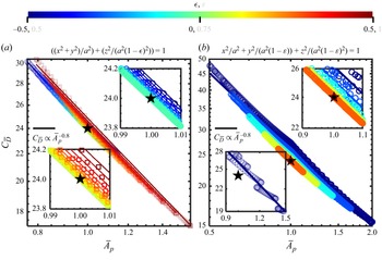
 CD¯
CD¯ A¯p
A¯p ϵ∈[−0.5,0.5]
 ε∈[0.5,1]
 CD¯∝A¯p−0.8
 (A¯p,CD¯)=(1,24)
 0<ϵ<0.5
 −0.5<ϵ<0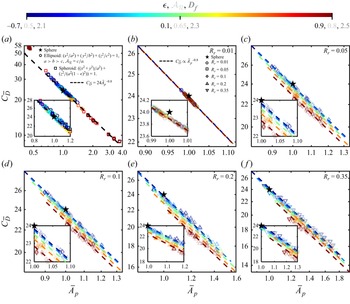
 CD¯
CD¯ A¯p
A¯p Rr
Rr CD¯∝A¯p−0.8
 ϵ∈[−0.7,0.9]
 AR∈[0.5,0.8]
 Df∈[2.1,2.5]
 x
x [0.9minA¯p,1.1maxA¯p]
 (A¯p,CD¯)=(1,24)
 CD¯
CD¯ y=x
y=x p1
p1 p2
p2 p2
p2 p3
p3
 Ps
Ps CD¯
CD¯ CD¯f
CD¯f CD¯p
CD¯p Rr
Rr Df
Df Rr
Rr p1
p1 p2
p2 p2
p2 p3
p3
 Ps
Ps A¯p
A¯p CD¯
CD¯ Df
Df Rr
Rr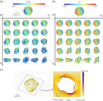
 τ⋅nx
τ⋅nx p
p τ⋅nx
τ⋅nx p
p Df=2.4
 Rr=0.1
 x
x y
y
 Pc
Pc Δτx
Δτx Δpx
Δpx 3U∞μfdeq
 Rr
Rr Df
Df Rr
Rr Df
Df Rr
Rr Pc=50%
 Δτx=0
Δτx=0 Δpx=0
Δpx=0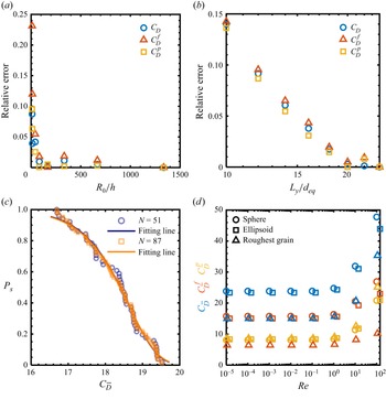
 Df=2.5
 Rr=0.2
 Ar=0.6023
 Df=2.5
 Rr=0.35
 Ar
Ar
 Ei
Ei
 Fi
Fi
 R
R
 S
S
 CX
CX
 AR
AR


 a
a


 Df=2.5
 Rr=0.35
 Ar=2.5
 Ar=0.7
 Ar=1.7

 Ps
Ps CL¯
CL¯ CL¯f
CL¯f CL¯p
CL¯p Rr
Rr Df
Df Rr
Rr
 λp
λp
 Ps
Ps Ap
Ap a>b>c
a>b>c b/a=0.1
 0.3
0.3 0.5
0.5 0.7
0.7 0.9
0.9 c/b
c/b Ps(Ap)=e−(Ap/λ)k
 kp
kp
 Open access

