


1. Introduction
The flow past bluff bodies has been considered in extensive engineering applications because of its strong interaction between the viscous and inviscid regions representing the realistic flow features, helping explore the drag reduction, stability, etc. Generally, aerodynamic studies of symmetric bodies assume the presence of symmetric flows. However, the surrounding flow of a notchback car observed by Cogotti (Reference Cogotti1986) suggests a symmetry breaking of the wake, showing switches between two asymmetric mirrored states. The bi-stability characterized by stochastic wake reversals behind notchback sedan models has been repeatedly observed also by Lawson, Garry & Faucompret (Reference Lawson, Garry and Faucompret2007), Wieser et al. (Reference Wieser, Schmidt, Mueller, Strangfeld, Nayeri and Paschereit2014) and Yan et al. (Reference Yan, Xia, Zhou, Zhu and Yang2019).
Not only sedans but also a car-like bluff body, the notchback Ahmed body, was found to produce wake asymmetry (Sims-Williams, Marwood & Sprot Reference Sims-Williams, Marwood and Sprot2011). The wake bi-stability of the notchback geometry was confirmed, for the first time numerically, by He et al. (Reference He, Minelli, Wang, Dong, Gao and Krajnović2021a) using large-eddy simulations (LES). A notchback Ahmed body maintains the frontal rounded surface of the original hatchback Ahmed body (Ahmed, Ramm & Faltin Reference Ahmed, Ramm and Faltin1984) but with a trunk attached to the rear body. It is worth noting that the wake asymmetry has been observed for the squareback Ahmed body (Grandemange, Cadot & Gohlke Reference Grandemange, Cadot and Gohlke2012; Grandemange, Gohlke & Cadot Reference Grandemange, Gohlke and Cadot2013a,Reference Grandemange, Gohlke and Cadotb). Particularly, as observed in the experiment (Grandemange et al. Reference Grandemange, Cadot and Gohlke2012) and later confirmed in LES (Evstafyeva, Morgans & Dalla Longa Reference Evstafyeva, Morgans and Dalla Longa2017), the presence of the symmetry breaking was found to depend on the Reynolds number in the laminar regime. The wake asymmetry persisting to the turbulent regime observed by Grandemange et al. (Reference Grandemange, Gohlke and Cadot2013a,Reference Grandemange, Gohlke and Cadotb) showed bi-stability characterized by stochastic switches of two mirrored asymmetric states.
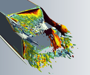
So far, the wake bi-stability of the squareback body has been investigated extensively. However, the notchback configuration allowing the flow reattachment to the trunk is different from wake separations of a squareback body. Therefore, the wake bi-stability behind a notchback body deserves further investigation. The wake, particularly in the separation and reattachment region of the notchback car, has been found to be sensitive to the Reynolds number (Gilhome, Saunders & Sheridan Reference Gilhome, Saunders and Sheridan2001). Besides, bi-stable wake states with separation bubbles attached to the slanted rear were observed behind a slanted cylinder afterbody (Zigunov, Sellappan & Alvi Reference Zigunov, Sellappan and Alvi2020). In this work, the bi-stability was only found at a lower Reynolds number,  $Re=2.5 \times 10^{4}$. With higher Reynolds numbers, the separation bubble length was reduced, and the bi-stable phenomenon was not reported. Therefore, it can be deduced that the Reynolds number influences the wake state with slanted rears.
Although the wake bi-stability behind slanted rears has been reported in the literature, the underlying mechanism of the Reynolds number influence remains unclear. For this reason, the present work aims to investigate the instability of the bi-stable wake behind a notchback bluff body under the Reynolds number influence by performing both experiments and numerical simulations. The authors believe that the results of the present paper bring new insight into the natural wake bi-stability and help promote the understanding of the notchback body flow.
The manuscript is organized as follows. Section 2 presents the description of the numerical and experiment methods. In § 3, the results are analysed with the focus on the Reynolds number influence on the state instability of the bi-stable wake. Conclusions follow in § 4. The mesh resolution and validation are presented in the Appendix.
2. Methodology
2.1. Description of numerical simulations
The investigated geometry is a notchback Ahmed body. The wake of this body is expected to be bi-stable as previously observed by Sims-Williams et al. (Reference Sims-Williams, Marwood and Sprot2011). The model dimensions expressed in the body height,  $H=0.096$ m, are presented in figure 1. The body width is
  $W=1.35H$, and the length is
  $L=3.82H$. The afterbody is characterized as a notchback configuration, presenting a slant and a deck. The deck length is
  $L_{D}=0.469H$, and the deck height is
  $H_{D}=0.687H$. The effective backlight angle is
  $\beta =17.8^{\circ }$, allowing the roof length
  $L_{S}=2.847H$. The body is suspended off the ground with a ground clearance of
  $H_{C}=0.21H$. The model is placed in the central width of a computation tunnel, under zero yaw angle, with the tunnel width
  $W_{T}=11.46H$ and the height
  $H_{T}=5.73H$. The inlet is set as a uniform inlet velocity profile, located at
  $8H$ upstream of the model. The pressure outlet with a constant 0 Pa is set at
  $19H$ downstream of the model. The lateral surfaces and the roof are set as symmetry planes. The no-slip wall is applied to the surface of the model and the ground.
The geometric model: (a) side view, (b) front view.

The governing LES equations are solved with the commercial finite volume solver, Star CCM+ 2019.2. The subgrid eddies are modelled by the wall-adapting local eddy-viscosity (WALE) model (Nicoud & Ducros Reference Nicoud and Ducros1999). Convective fluxes are approximated by a blend of 98 % central difference scheme of second-order accuracy and 2 % upwind scheme. The time integration is done using the second-order accurate three-level time Euler scheme. The Reynolds-averaged Navier–Stokes (RANS) approach is first employed for the initial condition. An initial time  $t^{*}=t U_{i n f} / H=62$ (t is the simulation time, Uinf is the free stream velocity) corresponding to two flow-through passages through the domain is considered for the physical establishment of the flow for LES. Then, the data are sampled at the last of 12 iterations in each time step with a sampling duration of
  $t^{*}=124$. The time step set-up, mesh resolution and validation are presented in the Appendix. The numerical method used in the present work has been applied to the studied flow by the same authors in He et al. (Reference He, Minelli, Wang, Dong, Gao and Krajnović2021a,Reference He, Minelli, Wang, Gao and Krajnovićb,Reference He, Minelli, Wang, Gao and Krajnovićc).
2.2. Experimental set-up
Experiments are carried out in the closed-circuit wind tunnel at Chalmers University of Technology. The flow turbulence level is within 0.15 % at a frequency range of 1 to 10 000 Hz. The tested model has a height  $H^{*}=2 H=0.192$ m, giving the same shape as the model used in the simulation but twice as large. The model is mounted in a test section of
  $6.5 H^{*} \times 9.4 H^{*} \times 15.6 H^{*}$ (height
  $\times$ width
  $\times$ length) with a ground clearance of
  $0.21 H^{*}$. The body is supported by four vertical cylinders with a diameter of
  $0.1H^{*}$.
The model is equipped with pressure taps on the rear body. The pressure is obtained using a Scanivalve system (NetScanner TM model 9116). This system has an accuracy of  ${\pm }$0.2 Pa for the used pressure range (
 ${\pm }$300 Pa) with a sampling frequency of 62.5 Hz. The hot-wire is mounted on a computer-controlled three-dimensional traversing mechanism to characterize the flow frequency. The hot-wire is connected to a constant temperature circuit (Dantec 56C01 CTA) with an over-heat ratio of 1.7. The velocity signal is filtered at a cutoff frequency of 20 000 Hz and digitized at a sampling frequency of 10 000 Hz, giving a reliable real frequency range between 5 and 5000 Hz.
3. Analysis and discussion
3.1. The flow state of bi-stability
The flow state under the Reynolds number influence observed in the wind tunnel experiment is discussed in this section. For the notchback Ahmed body, the asymmetric flow reattachment on the deck leads to the pressure difference on the two sides (He et al. Reference He, Minelli, Wang, Dong, Gao and Krajnović2021a). To obtain the pressure signals, two monitoring points,  $P_{dl}$ and
  $P_{dr}$, are set on the deck (figure 2a). The distance between the central line and each point is
  ${\textrm {d}}y=0.417 H^{*}$. The points are at
  $D_{P 2}=0.5 L_{D}^{*}$ from the deck's trailing edge, where
  $L_{D}^{*}=0.469 H^{*}$ is the deck length. Therefore, the asymmetry degree can be quantified by the deck pressure gradient, defined as
 \begin{equation} \frac{\partial C_{p d}}{\partial y}=\frac{C_{p}\left(P_{d r}\right)-C_{p}\left(P_{d l}\right)}{2 {\textrm{d}y}/H}, \end{equation}
where  $C_{p}$( ) represents the sampled pressure coefficient on each monitoring point. By the definition, a higher absolute value of
  $\partial C_{p d} / \partial y$ indicates a higher degree of wake asymmetry.
Pressure gradients,  $\partial C_{pd} / \partial y$. (a) Pressure taps on the deck. (b) The normalized p.d.f. of
  $\partial C_{pd} / \partial y$ as a function of
  $Re$. (c–f) Time history of
  $\partial C_{pd} / \partial y$ with p.d.f.: (c)
  $Re=5 \times 10^{4}$, (d)
  $Re=10 \times 10^{4}$, (e)
  $Re=15 \times 10^{4}$, (f)
  $Re=20 \times 10^{4}$.

Figure 2(b) presents the normalized probability density function (p.d.f.) of  $\partial C_{p d} /\partial y$ as a function of the Reynolds number,
  $Re$. The value of
  $Re$ is based on the free stream velocity,
  $U_{inf}$, and the body height,
  $H$. Data are sampled from
  $Re=5 \times 10^{4}$ to
  $Re=25 \times 10^{4}$ with the interval of
  $Re=2.5 \times 10^{4}$. For each case, the sampling time is over
  $1.8 \times 10^{3}$ s.
At the low  $Re$ region with
  $Re \leq 10 \times 10^{4}$,
  $\partial C_{p d} / \partial y$ concentrates at both negative and positive values. This means that the statistic wake undergoes two asymmetric states. In figure 2(c,d), for
 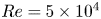 $Re=5 \times 10^{4}$ and
  $Re=10 \times 10^{4}$, the wake bi-stability is characterized as
  $\partial C_{p d} / \partial y$ stochastically switches between the two states,
  $S_{A}$ and
  $S_{B}$. The two states are considered to be mirrored since the absolute values of
  $\partial C_{p d} / \partial y$ during
  $S_{A}$ and
  $S_{B}$ are similar. Under the low
  $Re$, the higher amplitude of the
  $\partial C_{p d} / \partial y$ fluctuation indicates a lower accuracy because the ratio of the measuring deviation to pressure signals is higher.
For  $12.5 \times 10^{4} \leq Re \leq 17.5 \times 10^{4}$,
  $\partial C_{pd} / \partial y$ not only concentrates with negative and positive values but also in the centre region approaching zero. Thus, the wake seems to be ‘tri-stable’. For example, in figure 2(e), under
 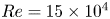 $Re=15 \times 10^{4}$,
  $\partial C_{p d} / \partial y$ undergoes
  $S_{A}$,
  $S_{B}$ and the symmetric state,
  $S_{C}$. As the Reynolds number increases further, the proportion of
  $S_{C}$ gradually increases. For
 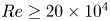 $Re \geq 20 \times 10^{4}$, the wake seems symmetrized as
  $\partial C_{pd} / \partial y$ remains in the centre. Shown in figure 2(f) is that
  $S_{C}$ becomes dominant among the three states. Looking at figure 2(a), for
 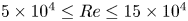 $5 \times 10^{4} \leq Re \leq 15 \times 10^{4}$, the degree of the asymmetry gradually increases with the higher Reynolds number since the absolute values of the positive and negative peaks become higher. Furthermore, comparing figure 2(c–f), it can be observed that the wake switches more frequently with a higher
  $Re$, increasing the proportion of
  $S_{C}$.
Although  $\partial C_{pd} / \partial y$ presented in figure 2 can be analysed regarding the bi-stability, its fluctuation, particularly at the higher
  $Re$, interferes with the distinction between the wake states. When the signal of
  $\partial C_{pd} / \partial y$ is filtered with an average filter over windows of 0.5 s, like examples shown in figure 3, the interference of the fluctuation reduces. Therefore, the wake states can be quantitatively depicted. When the wake is in the asymmetric state,
  $\overline {\partial C_{p d} / \partial y}$ corresponding to
  ${\pm }$0.62 and
  ${\pm }$0.8 are respectively observed for
  $Re=5 \times 10^{4}$ and
  $Re=20 \times 10^{4}$. To distinguish the wake states, the dash lines at
  $\partial C_{pd} / \partial y=\pm 0.31$ (figure 3a) and
  $\partial C_{pd} / \partial y=\pm 0.4$ (figure 3b) are employed as the boundary lines.
Time history of  $\partial C_{pd} / \partial y$. The black line is the signal obtained from the pressure monitors. The red line is the filtered signal using an averaging filter over windows of 0.5 s. (a)
  $Re=5 \times 10^{4}$, (b)
  $Re=20 \times 10^{4}$.

Inspired by Grandemange et al. (Reference Grandemange, Gohlke and Cadot2013a), the statistics of the bi-stable states are analysed by the probability distribution. For example, the conditional probability obtained under  $Re=5 \times 10^{4}$ and
  $Re=20 \times 10^{4}$ is listed in table 1. At the low
  $Re$,
$Re$,  $S_{A}$ and
  $S_{B}$ states are dominant, and the wake tends to maintain the current asymmetric state. However, at the high
  $Re$, the proportion of
  $S_{C}$ becomes higher, leading the
  $S_{A}$ and
  $S_{B}$ states to be more unstable.
Probabilities of the current wake state,  $S_{t}$, depending on the previous states,
  $S_{t-1}$.
  $P(E_{1}=E_{2})$ is the conditional probability of the event
  $E_{1}$, given by the event
  $E_{2}$. The events are considered at 0.5 Hz.

To study the instability of the wake states, the probability distribution of the wake switch is investigated. Assuming  $P_{{switch }}=P(S_{t} \neq S_{t-1})$,
  $S_{t-1} \in (S_{A}, S_{B})$ to be the switching rate independent of the instant
  $t$. Therefore,
  $P_{{switch }}=0.0147$ for
  $Re=5 \times 10^{4}$ and
  $P_{{switch }}=0.0741$ for
  $Re=20 \times 10^{4}$ can be given by the results listed in table 1 with
 $$\begin{gather} P_{{switch }}=P\left(S_{t}=S_{A}\right)\left[1-P\left(S_{t}=S_{A} \mid S_{t-1}=S_{A}\right)\right]\nonumber\\ +P\left(S_{t}=S_{B}\right)\left[1-P\left(S_{t}=S_{B} \mid S_{t-1}=S_{B}\right)\right]. \end{gather}$$
Note that the switching event considered in (3.2) considers the possibility of the asymmetry breaking, describing the wake shifting from an asymmetric state to  $S_{C}$ or directly to the opposite asymmetric state. In most instances, the wake undergoes the
  $S_{C}$ state during the switching process. However, the wake shifting from the asymmetric state to
  $S_{C}$ does not ensure a successful switch to the opposite asymmetric state. Sometimes the wake returns from
  $S_{C}$ to the initial asymmetric state, presenting an attempt to switch. This phenomenon has been discussed by He et al. (Reference He, Minelli, Wang, Dong, Gao and Krajnović2021a). Therefore, (3.2) counts both the successful and unsuccessful switches since the attempt to switch also breaks the asymmetric state.
Taking into account the events considered at 0.5 Hz, the dimension of  $P_{{switch }}$ can be considered as ‘per 0.5 s’. Thus, the expected value of the duration (in seconds) for the wake state can be represented by the reciprocal of 2
 $P_{{switch }}$. Assuming that when not switching, the wake is possibly in one of the asymmetric states or in the
  $S_{C}$ state. Thus, the expected value of the duration time for the asymmetric state needs to eliminate the interference of
  $S_{C}$, given by
 \begin{equation} T_{m}=\frac{1-P\left(S_{t}=S_{C}\right)}{2P_{{switch }}}. \end{equation}
Applying (3.3) for all tested  $Re$,
$Re$,  $T_{m}$ is a function of
  $Re$ following an exponential law illustrated in figure 4. The
  $T_{m}$ for each Reynolds number is obtained from the pressure signals monitored over
  $1.8 \times 10^{3}$ s, using an averaging filter over windows of 0.5 s. The standard deviations of
  $T_{m}$ are calculated with window lengths of
  $3 \times 10^{2}$ s. It can be seen that
  $T_{m}$ decreases with higher
  $Re$. Moreover, under the low
  $Re$, the standard deviations are higher since the asymmetric state can be maintained possibly from a few seconds to tens of seconds.
The expected value of the duration time for the asymmetric state as a function of Reynolds number.

The duration time of the asymmetric state reduces with increasing  $Re$ symmetrizing the wake. Therefore, exploring the instability of the symmetric state requires an examination under small yaws. For the wake bi-stability behind the squareback body, the discontinuous transition between the two mirrored wake states has been observed under a small yawing angle (Cadot, Evrard & Pastur Reference Cadot, Evrard and Pastur2015; Volpe, Devinant & Kourta Reference Volpe, Devinant and Kourta2015; Bonnavion & Cadot Reference Bonnavion and Cadot2018). The wake state was found extremely sensitive to the change of very small angles, showing a phase jump between the positive and negative yaw angles. Similarly, for the notchback case, the wake is sensitive to small yaw angles, showing in the experiment a phase jump around zero yaws. As shown in figure 5, under
 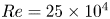 $Re=25 \times 10^{4}$, the model placed at zero yaws presents the fluctuation of
  $\partial C_{pd} / \partial y$ around 0, indicating wake symmetry. However, under positive or negative small yaw angles,
  $\partial C_{pd} / \partial y$ stays respectively in positive or negative regions, suggesting asymmetry. Therefore, for the notchback body, the symmetry of the wake at high
  $Re$ remains unstable. This means that the wake still has the bi-stable nature, being different from general symmetric flows of symmetric bluff bodies.
The time history of the deck pressure gradient under yaws: (a)  ${\rm yaw}=0^{\circ }$, (b)
  ${\rm yaw}=0.5^{\circ }$, (c)
  ${\rm yaw}=-0.5^{\circ }$. Data obtained under
  $Re=25 \times 10^{4}$.

3.2. The flow structures
In order to identify the flow structures and explore the underlying mechanism of the switch depending on  $Re$, numerical simulations using LES are performed at
  $Re=5 \times 10^{4}$,
  $Re=15 \times 10^{4}$ and
  $Re=20 \times 10^{4}$. The wake asymmetry is predicted in all three cases, but the wake switch is not observed due to the limitation of the simulations to simulate sufficiently long physical time. For example, for
  $Re=20 \times 10^{4}$, the present experiment suggests that the expected period of the asymmetric state estimated by (3.3) is
  $T_{m}=2.189\,\textrm {s}$. Although the numerical simulation considering the flow averaged for
  $t^{*}=124$ corresponding to four flow-through passages through the domain, the physical time
  $t=t^{*}H/U_{inf}=0.38$ s is much shorter than
  $T_{m}$. However, the wake bi-stability is observed since the case of
  $Re=5 \times 10^{4}$ is in the
  $S_{B}$ state, but the other two cases show the
  $S_{A}$ state due to the random appearance of asymmetric states. For clarity, the numerical results are presented in the same normalized state by mirroring
  $S_{A}$ to
  $S_{B}$.
The distribution of the mean streamlines and the spanwise vorticity,  $\overline {\varOmega _{y}}$, projected on the section planes,
  $Y_{1}$ and
  $Y_{2}$, are presented in figure 6. The vorticity is normalized with
  $U_{inf}$ and
  $H$. The wake separation can be identified by
  $\overline {\varOmega _{y}}$, showing the vortex
  $V_{c}$ separating from the near-wall region of the roof,
  $V_{b}$ from the deck's trailing edge and
  $V_{g}$ from the bottom body. The flow reattaching to the deck is indicated in the streamlines. For quantitative analysis,
  $L_{VC}$ indicating the separation length of
  $V_{c}$ is defined as the distance between the roof and the local maximum
  $x$-coordinate on the contour line of
  $\overline {\varOmega _{y}}=3.7$. The reattachment length
  $L_{R}$ is defined as the distance between the positive–negative transition point of near-wall
  $\overline {\varOmega _{y}}$ and the deck's trailing edge. The asymmetry of the mean flow is predicted in the three cases. The readers are referred to He et al. (Reference He, Minelli, Wang, Dong, Gao and Krajnović2021a) for details of the asymmetric flow structures behind the notchback Ahmed body.
Mean streamlines and spanwise vorticity  $\overline {\varOmega _{y}}$ on the
  $Y_{1}$ and
  $Y_{2}$ planes. Here
  $Y_{1}$ and
  $Y_{2}$ are symmetric to the central section and the distance between
  $Y_{1}$ and
  $Y_{2}$ is
  $D_{P3}$=0.5
 $W$ (half-width of the model). (a,b)
  $Re=5 \times 10^{4}$, (c,d)
  $Re=15 \times 10^{4}$, (e,f)
  $Re=20 \times 10^{4}$.

Focusing on the notchback region, the flow structures projected on the horizontal  $Z_{1}$ plane behind the rear slant are presented in figure 7. The distribution of the mean streamwise velocity,
  $\bar {u}$, normalized by
  $U_{inf}$, is shown in figure 7(a–c). For the three cases, the flow structure
  $V_{c}$ deflecting to the left-hand side indicates asymmetry. Therefore, the C-pillar vortex on the left-hand side is disturbed by
  $V_{c}$. On the other hand, the right C-pillar vortex,
  $V_{r}$, extends further downstream. The similarity of the
  $\bar {u}$ field can be quantitated by the profile on the probe line,
  $L_{p}$, illustrated in figure 7(j).
Flow structures projected on the  $Z_{1}$ plane, located at
  $H_{P1}=0.844H$ above the bottom of the model. (a–c) Distribution of
  $\bar {u}$. (d–f) Mode 2 of POD. (g–i) Distribution of TKE. For (a–i), the left, the middle and the right columns are at
  $Re=5 \times 10^{4}$,
  $Re=15 \times 10^{4}$ and
  $Re=20 \times 10^{4}$, respectively. Profiles on the probe line,
  $L_{p}$, at
  $D_{P1}=0.3H$ from the slant: (j)
  $\bar {u}$, (k) TKE.

The wake dynamics is identified by the modal analysis using the proper orthogonal decomposition (POD). As originally proposed by Lumley (Reference Lumley1970), and later introduced with the method of snapshots by Sirovich (Reference Sirovich1987), the POD method is based on the energy ranking of orthogonal structures predicted from a correlation matrix of the snapshots. A singular value decomposition (SVD) approach is used for the POD analysis. The POD method applied to the pressure snapshots in the  $Z_{1}$ plane recognizes the modes of the flow structures based on the energy content. This approach has been successfully used for the studied flow in previous published works by the same author (He et al. Reference He, Minelli, Wang, Dong, Gao and Krajnović2021a,Reference He, Minelli, Wang, Gao and Krajnovićb). The mean field contributes to Mode 1 containing most of the energy. The wave packets presented in figure 7(d–f) are identified by Mode 2 ranking the second energy content. The three cases are consistent, showing
  $V_{c}$ moving downstream on the left-hand side, following the left deflection of
  $V_{c}$.Therefore, the flow structures and wake dynamics are not evidently influenced by the higher
  $Re$.
$Re$.
However, large differences are found in the distribution of turbulence kinetic energy (TKE) presented in figure 7(g–i). Under  $Re=5 \times 10^{4}$, TKE in the wake is lower. For the two cases with the higher
  $Re$, TKE increases sharply. The distinction of TKE is quantitated by the profiles shown in figure 7(k). Compared with the two high
  $Re$ cases, TKE is much lower with the low
  $Re$. Therefore, the wake with a higher
  $Re$ is more turbulent. For the wake bi-stability behind the squareback Ahmed body, literature has shown the sensitivity to the underbody (Barros et al. Reference Barros, Borée, Cadot, Spohn and Noack2017) or the background (Burton et al. Reference Burton, Wang, Smith, Scott, Crouch and Thompson2017) turbulence. Therefore, it can be deduced that the high turbulent wake for the notchback case leads to unsteadiness, resulting in the higher possibility to break the asymmetric state. For this reason, the wake switching frequency increases with the higher
  $Re$, culminating in the higher proportion of
  $S_{C}$ observed in the experiment.
4. Conclusions
The bi-stable flow past a notchback Ahmed body is investigated by wind tunnel experiments and LES. The Reynolds number influence on the wake instability is analysed. Experimental results suggest that for  $Re \leq 10\times 10^{4}$, the wake is bi-stable with low-frequency switches. For
  $12.5 \times 10^{4} \leq Re \leq 17.5 \times 10^{4}$, the wake becomes ‘tri-stable’ due to the presence of a symmetric state. With
  $Re$ increasing further, the proportion of the symmetric state increases, symmetrizing the bi-stable flow.
The wake switching frequency is assessed by calculating the conditional probability of the wake states observed in experiments. A higher frequency of the switch between two mirrored states is found with increasing  $Re$, leading the duration time of the asymmetric state to decrease following an exponential law. Therefore, the increasing proportion of the symmetric state under higher
  $Re$ is attributed to highly frequent wake switches. The symmetric state at high
  $Re$ still has the bi-stable feature since the unstable wake remains sensitive to small yaw angles approaching zero.
The wake asymmetry is confirmed in the LES at  $Re=5 \times 10^{4}$,
  $Re=15 \times 10^{4}$ and
  $Re=20 \times 10^{4}$. The consistency of the asymmetric wake is indicated by the wake separation, the reattachment and the wake dynamics identified by POD. However, the turbulence level is found significantly higher in the two higher
  $Re$ cases. Therefore, a higher turbulent wake is considered to trigger a higher possibility to break the asymmetric state, increasing the wake switching frequency, which in turn produces a higher proportion of the symmetric state.
Acknowledgements
Computations were performed at SNIC (Swedish National Infrastructure for Computing) at the National Supercomputer Center (NSC) at LiU. The authors thank Professor V. Chernoray, Mr I. Jonsson and Mr E. Hadziavdic for their help with the wind tunnel experiment conducted at Chalmers Laboratory of Fluids and Thermal Science. The authors are grateful to the anonymous reviewers for their careful reading of the present manuscript and helpful comments.
Funding
K.H. acknowledges the financial support from China Scholarship Council, grant number: 201906370096.
Declaration of interests
The authors report no conflict of interest.
Appendix. Mesh resolution and validation
The multi-block hexahedral conforming computational grids are built using the Pointwise grids generator. The mesh resolutions are presented in table 2. The applicability of these mesh resolutions for the studied flow, established by a grid independence examination, has been discussed in the previous work (He et al. Reference He, Minelli, Wang, Gao and Krajnović2021b). For the higher  $Re$ case, to keep the wall-normal resolution
  $n^{+}<1$ and fulfil the requirement of the streamwise resolution
  $\Delta_{s}^{+}$ and the spanwise resolution
  $\Delta_{l}^{+}$, smaller computational cells are used, leading to a higher number of cells. The non-dimensional time step is
  $\textrm {d}t^{*}=\Delta t_{s} U_{i n f} / H=3.44 \times 10^{-3}$ for
  $Re=5 \times 10^{4}$,
  $\textrm {d} t^{*}=1.15 \times 10^{-3}$ for
  $Re=15 \times 10^{4}$ and
  $\textrm {d} t^{*}=8.6 \times 10^{-4}$ for
  $Re=20 \times 10^{4}$, allowing the Courant–Friedrichs–Lewy number for all simulations being lower than one in over 99 % of the cells during all time steps.
Spatial resolutions of the grids.

Comparison of  $\overline {\partial C_{pd} / \partial y}$ between experiments and LES.

The present LES is validated by comparing it to the experimental results. For the experiment, the wake frequency is obtained from velocity signals sampled by a hot-wire. The measuring point is placed at  $0.1{H}^*$ behind the half-height of the C-pillar (the one which is not disturbed by the deflection of
  $V_{c}$ during the asymmetric state). The asymmetric wake state for sampling is identified by
  $\partial C_{pd} / \partial y$. The velocity and pressure signals are sampled throughout 2 s during the asymmetric state. For the LES, the frequency is obtained from the velocity magnitude signals monitored at the position following the hot-wire measurement.
The comparison of  $\overline {\partial C_{pd} / \partial y}$ is presented in table 2. It can be seen that the pressure and the degree of the wake asymmetry obtained in LES are in good agreement with those observed in the experiment. Moreover, the comparison of the shedding frequency of the C-pillar vortex is presented in figure 8. The frequency spectrum is obtained by the fast Fourier transform. The non-dimensional frequency
  $F^+$ is the Strouhal number (
 $St_{H^*}$ for experiments and
  ${St_H}$ for LES) normalized with
  $U_{inf}$ and the model height. The peak values of the normalized power spectral density (PSD) illustrate that the main frequency observed in the experiment is in accordance with that obtained in LES. Therefore, the accuracy of the LES is established by the experimental validation.
Comparison of the shedding frequency of the C-pillar vortex between experiments and LES. (a)  $Re=5 \times 10^{4}$, (b)
  $Re=15 \times 10^{4}$, (c)
  $Re=20 \times 10^{4}$.


 Open access